ANALYSIS OF ALGORITHMS AND BIG-O CS16: Introduction to Algorithms & Data Structures Tuesday, January...

1

ANALYSIS OF ALGORITHMS AND BIG-O

CS16: Introduction to Algorithms & Data Structures

Tuesday, January 28, 2014

2

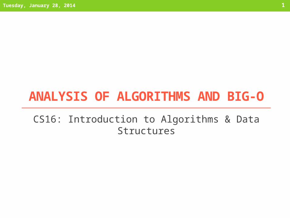
Outline

1) Running time and theoretical analysis

2) Big-O notation

3) Big-Ω and Big-Θ

4) Analyzing seamcarve runtime

5) Dynamic programming

6) Fibonacci sequence


3

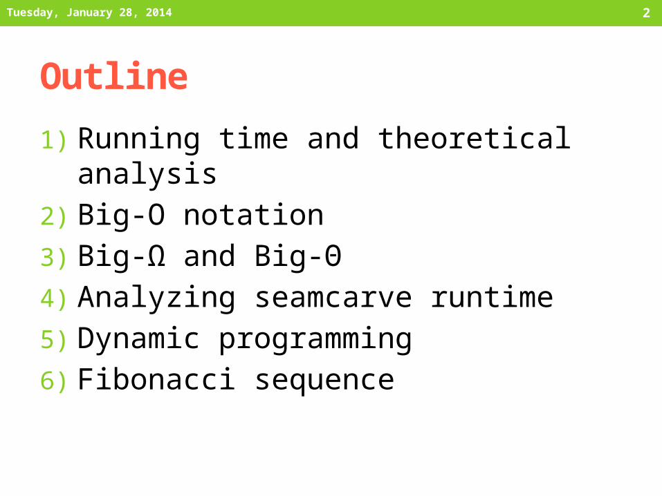
How fast is the seamcarve algorithm?

• What does it mean for an algorithm to be fast?• Low memory usage?• Small amount of time measured on a stopwatch?

• Low power consumption?

• We’ll revisit this question after developing the fundamentals of algorithm analysis


4

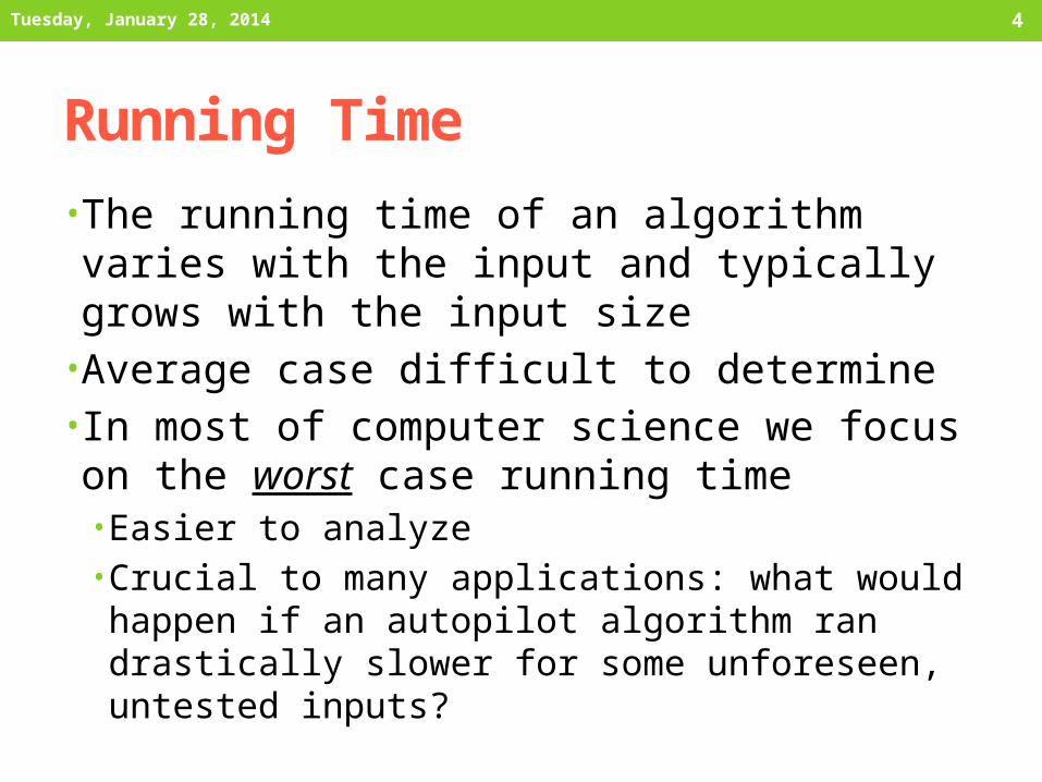
Running Time

• The running time of an algorithm varies with the input and typically grows with the input size

• Average case difficult to determine• In most of computer science we focus on the worst case running time• Easier to analyze• Crucial to many applications: what would happen if an autopilot algorithm ran drastically slower for some unforeseen, untested inputs?


5

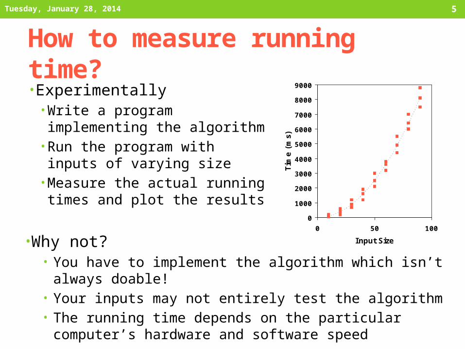
How to measure running time?• Experimentally

• Write a program implementing the algorithm

• Run the program with inputs of varying size

• Measure the actual running times and plot the results


0

1000

2000

3000

4000

5000

6000

7000

8000

9000

0 50 100

Input Size

Tim

e (

ms)

• Why not?• You have to implement the algorithm which isn’t always doable!• Your inputs may not entirely test the algorithm• The running time depends on the particular computer’s

hardware and software speed

6

Theoretical Analysis

• Uses a high-level description of the algorithm instead of an implementation

• Takes into account all possible inputs• Allows us to evaluate speed of an algorithm independent of the hardware or software environment

• By inspecting pseudocode, we can determine the number of statements executed by an algorithm as a function of the input size


7

Elementary Operations• Algorithmic “time” is measured in elementary operations

• Math (+, -, *, /, max, min, log, sin, cos, abs, ...)• Comparisons ( ==, >, <=, ...)• Function calls and value returns• Variable assignment• Variable increment or decrement• Array allocation• Creating a new object (careful, object's constructor may have

elementary ops too!)

• In practice, all of these operations take different amounts of time

• For the purpose of algorithm analysis, we assume each of these operations takes the same time: “1 operation”


8

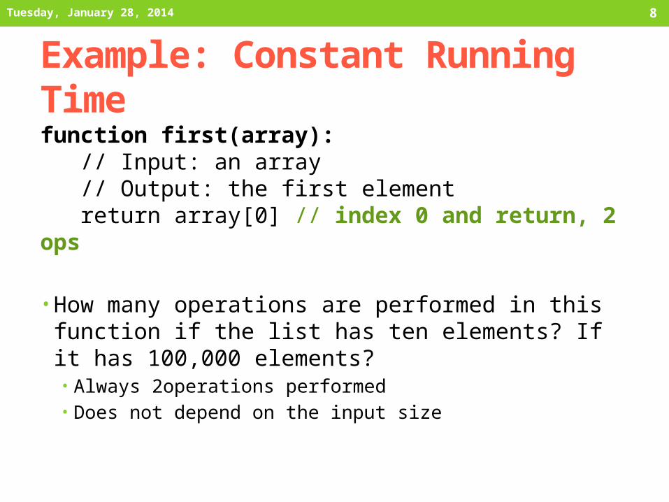
Example: Constant Running Time

function first(array): // Input: an array // Output: the first element return array[0] // index 0 and return, 2 ops

• How many operations are performed in this function if the list has ten elements? If it has 100,000 elements?• Always 2operations performed• Does not depend on the input size


9

Example: Linear Running Timefunction argmax(array): // Input: an array // Output: the index of the maximum value index = 0 // assignment, 1 op for i in [1, array.length): // 1 op per loop if array[i] > array[index]: // 3 ops per loop index = i // 1 op per loop, sometimes return index // 1 op

• How many operations if the list has ten elements? 100,000 elements?• Varies proportional to the size of the input list: 5n + 2• We’ll be in the for loop longer and longer as the input list grows• If we were to plot, the runtime would increase linearly


10

Example: Quadratic Running Timefunction possible_products(array): // Input: an array // Output: a list of all possible products // between any two elements in the list products = [] // make an empty list, 1 op for i in [0, array.length): // 1 op per loop for j in [0, array.length): // 1 op per loop per loop products.append(array[i] * array[j]) // 4 ops per loop per loop return products // 1 op

• Requires about 5n2 + n + 2 operations (okay to approximate!)• If we were to plot this, the number of operations executed grows quadratically!

• Consider adding one element to the list: the added element must be multiplied with every other element in the list

• Notice that the linear algorithm on the previous slide had only one for loop, while this quadratic one has two for loops, nested. What would be the highest-degree term (in number of operations) if there were three nested loops?


11

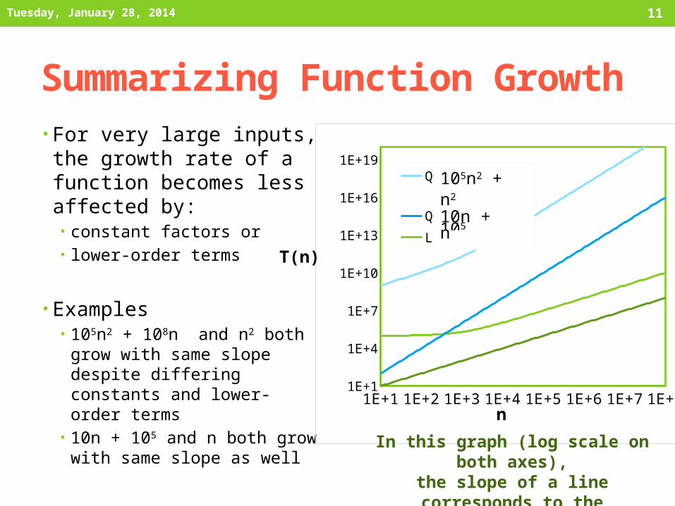
Summarizing Function Growth• For very large inputs, the

growth rate of a function becomes less affected by:• constant factors or• lower-order terms

• Examples• 105n2 + 108n and n2 both

grow with same slope despite differing constants and lower-order terms

• 10n + 105 and n both grow with same slope as well


1E+1 1E+2 1E+3 1E+4 1E+5 1E+6 1E+7 1E+81E+1

1E+4

1E+7

1E+10

1E+13

1E+16

1E+19Quadratic

Quadratic

Linear

Linear

105n2 + 108nn2

10n + 105n

In this graph (log scale on both axes),the slope of a line corresponds to thegrowth rate of its respective function

n

T(n)

12

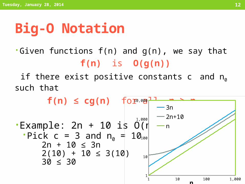
Big-O Notation

• Given functions f(n) and g(n), we say that f(n) is O(g(n)) if there exist positive constants c and n0 such that f(n) ≤ cg(n) for all n ≥ n0 • Example: 2n + 10 is O(n)

• Pick c = 3 and n0 = 102n + 10 ≤ 3n2(10) + 10 ≤ 3(10)30 ≤ 30


1 10 100 1,0001

10

100

1,000

10,000

3n

2n+10

n

n

13

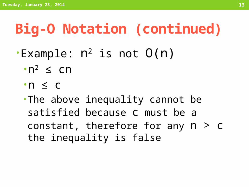
Big-O Notation (continued)

• Example: n2 is not O(n)• n2 ≤ cn• n ≤ c• The above inequality cannot be satisfied because c must be a constant, therefore for any n > c the inequality is false


14

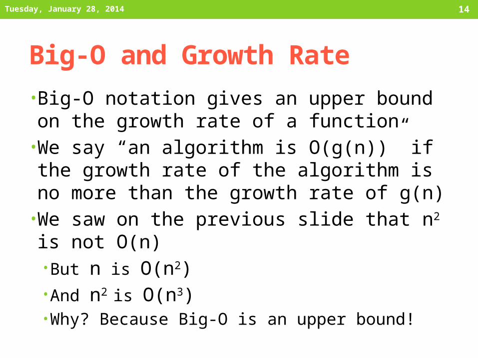
Big-O and Growth Rate

• Big-O notation gives an upper bound on the growth rate of a function

• We say “an algorithm is O(g(n))” if the growth rate of the algorithm is no more than the growth rate of g(n)

• We saw on the previous slide that n2 is not O(n)• But n is O(n2)• And n2 is O(n3)• Why? Because Big-O is an upper bound!


15

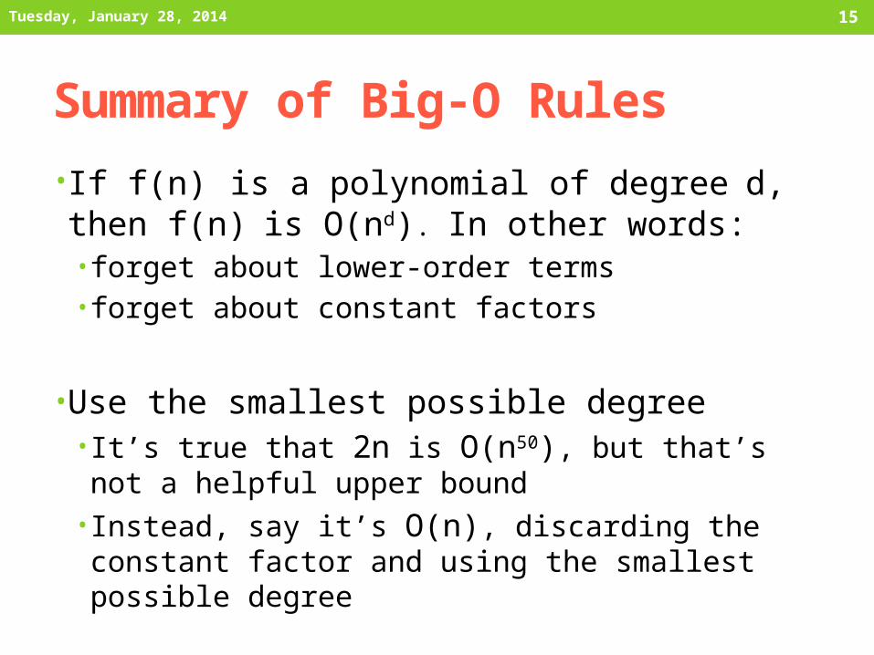
Summary of Big-O Rules

• If f(n) is a polynomial of degree d, then f(n)

is O(nd). In other words:• forget about lower-order terms• forget about constant factors

• Use the smallest possible degree• It’s true that 2n is O(n50), but that’s not a helpful upper bound

• Instead, say it’s O(n), discarding the constant factor and using the smallest possible degree


16

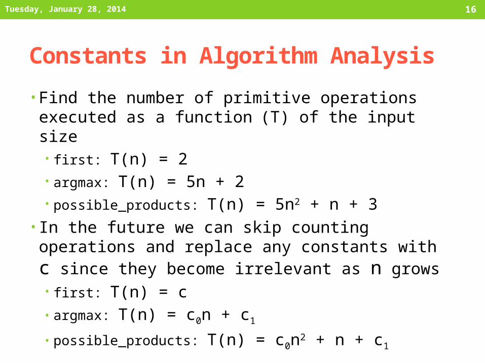
Constants in Algorithm Analysis• Find the number of primitive operations executed as a

function (T) of the input size• first: T(n) = 2• argmax: T(n) = 5n + 2• possible_products: T(n) = 5n2 + n + 3

• In the future we can skip counting operations and replace any constants with c since they become irrelevant as n grows• first: T(n) = c • argmax: T(n) = c0n + c1• possible_products: T(n) = c0n2 + n + c1


17

Big-Oin Algorithm Analysis

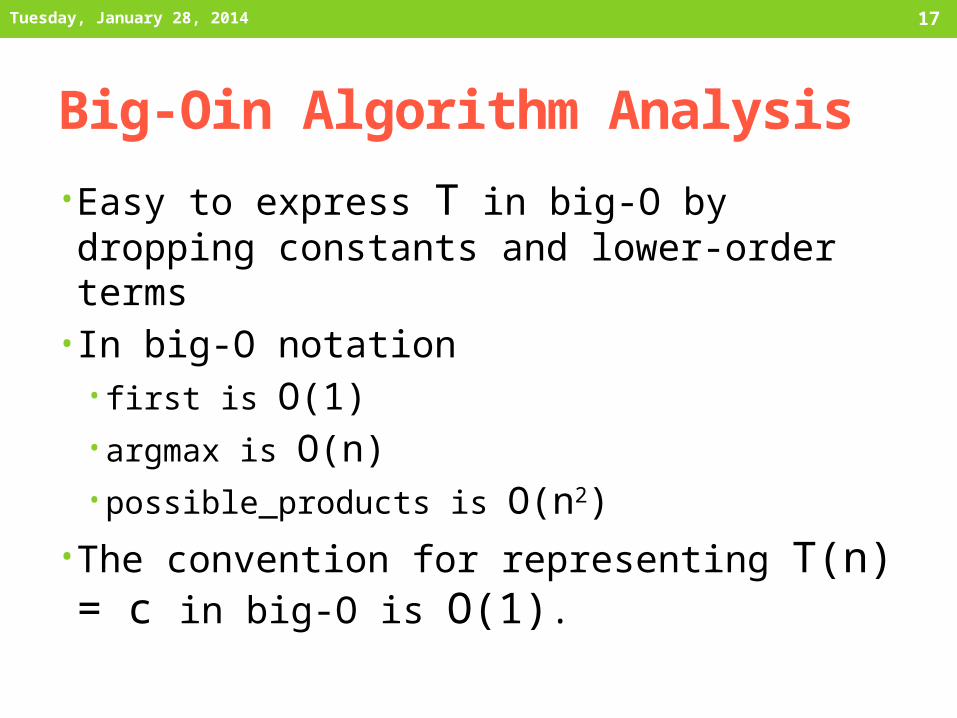
• Easy to express T in big-O by dropping constants and lower-order terms

• In big-O notation• first is O(1)• argmax is O(n)• possible_products is O(n2)

• The convention for representing T(n) = c in big-O is O(1).


18

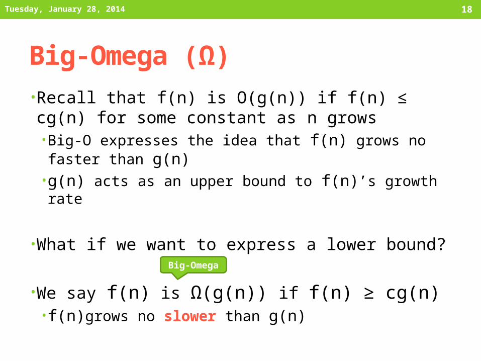
Big-Omega (Ω)

• Recall that f(n) is O(g(n)) if f(n) ≤ cg(n) for some constant as n grows• Big-O expresses the idea that f(n) grows no faster

than g(n)• g(n) acts as an upper bound to f(n)’s growth rate

• What if we want to express a lower bound?

• We say f(n) is Ω(g(n)) if f(n) ≥ cg(n)• f(n)grows no slower than g(n)


Big-Omega

19

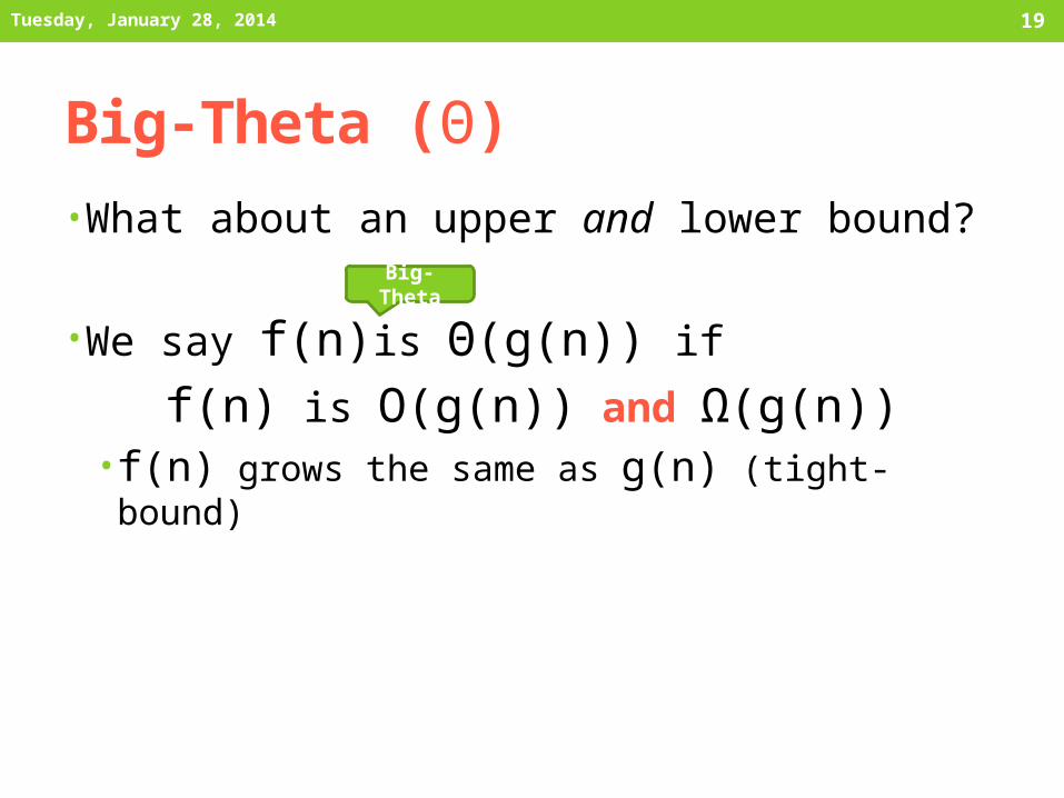
Big-Theta (Θ)

• What about an upper and lower bound?

• We say f(n)is Θ(g(n)) iff(n) is O(g(n)) and Ω(g(n))• f(n) grows the same as g(n) (tight-bound)


Big-Theta

20

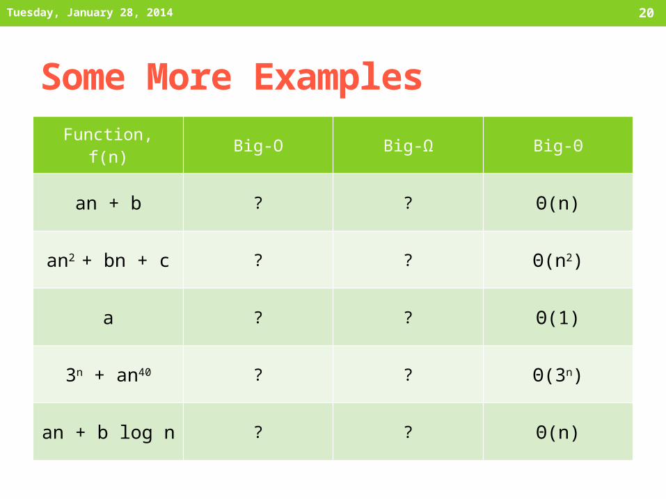
Some More Examples

Function, f(n) Big-O Big-Ω Big-Θ

an + b ? ? Θ(n)an2 + bn + c ? ? Θ(n2)

a ? ? Θ(1)3n + an40 ? ? Θ(3n)

an + b log n ? ? Θ(n)


21

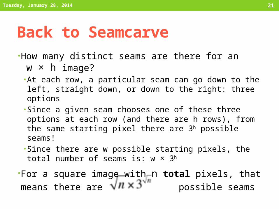
Back to Seamcarve

• How many distinct seams are there for an w × h image?• At each row, a particular seam can go down to the left,

straight down, or down to the right: three options• Since a given seam chooses one of these three options

at each row (and there are h rows), from the same starting pixel there are 3h possible seams!

• Since there are w possible starting pixels, the total number of seams is: w × 3h

• For a square image with n total pixels, that

means there are possible seams


22

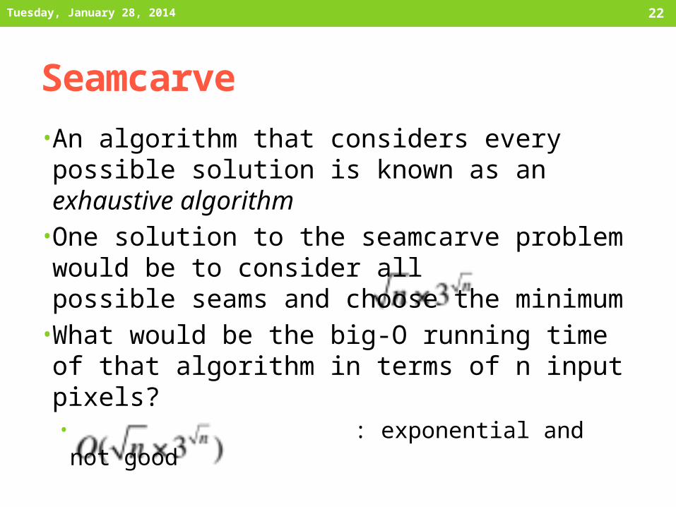
Seamcarve

• An algorithm that considers every possible solution is known as an exhaustive algorithm

• One solution to the seamcarve problem would be to consider all possible seams and choose the minimum

• What would be the big-O running time of that algorithm in terms of n input pixels?• : exponential and not good


23

Seamcarve• What’s the runtime of the solution we went over last

class?• Remember: constants don’t affect big-O runtime

• The algorithm:• Iterate over every pixel from bottom to top to populate the costs and dirs arrays

• Create a seam by choosing the minimum value in the top row and tracing downward

• How many times do we evaluate each pixel?• A constant number of times• Therefore the algorithm is linear, or O(n), where n is the

number of pixels

• Hint: we also could have looked back at the pseudocode and counted the number of nested loops!


24

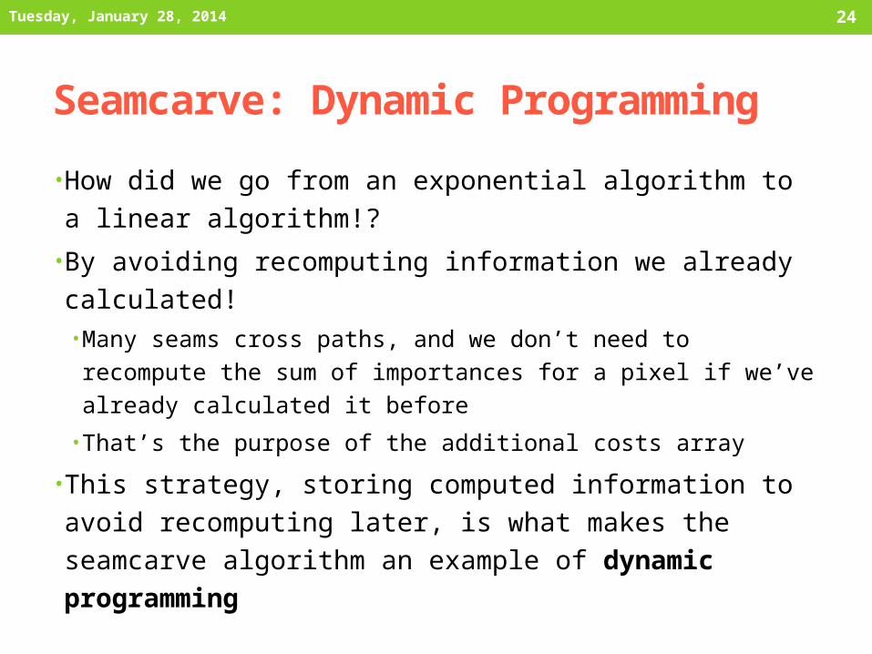
Seamcarve: Dynamic Programming

• How did we go from an exponential algorithm to a linear

algorithm!?

• By avoiding recomputing information we already

calculated!• Many seams cross paths, and we don’t need to recompute the

sum of importances for a pixel if we’ve already calculated it

before

• That’s the purpose of the additional costs array

• This strategy, storing computed information to avoid

recomputing later, is what makes the seamcarve

algorithm an example of dynamic programming


25

Fibonacci: Recursive0, 1, 1, 2, 3, 5, 8, 13, 21, 34, …

• The Fibonacci sequence is usually defined by the following recurrence relation:F0 = 0, F1 = 1Fn = Fn-1 + Fn-2

• This lends itself very well to a recursive function for finding the nth Fibonacci number


function fib(n): if n = 0: return 0 if n = 1: return 1 return fib(n-1) + fib(n-2)

26

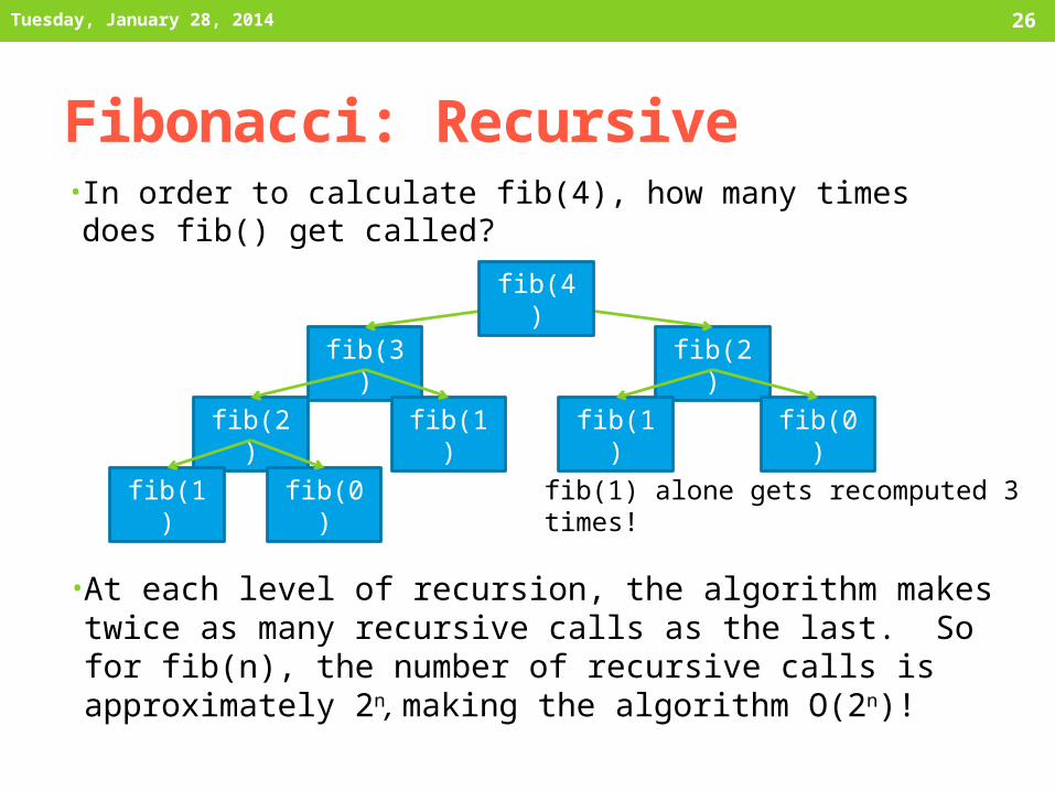
Fibonacci: Recursive• In order to calculate fib(4), how many times does fib() get called?


fib(3)

fib(2)

fib(2)

fib(1)

fib(1)

fib(0)

fib(1)

fib(0)

fib(4)

fib(1) alone gets recomputed 3 times!

• At each level of recursion, the algorithm makes twice as many recursive calls as the last. So for fib(n), the number of recursive calls is approximately 2n, making the algorithm O(2n)!

27

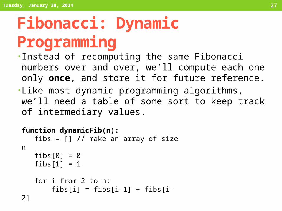
Fibonacci: Dynamic Programming• Instead of recomputing the same Fibonacci numbers

over and over, we’ll compute each one only once, and store it for future reference.

• Like most dynamic programming algorithms, we’ll need a table of some sort to keep track of intermediary values.


function dynamicFib(n): fibs = [] // make an array of size n fibs[0] = 0 fibs[1] = 1 for i from 2 to n: fibs[i] = fibs[i-1] + fibs[i-2]

return fibs[n]

28

Fibonacci: Dynamic Programming (2)

• What’s the runtime of dynamicFib()?

• Since it only performs a constant number of operations to calculate each fibonacci number from 0 to n, the runtime is clearly O(n).

• Once again, we have reduced the runtime of an algorithm from exponential to linear using dynamic programming!


29

Readings• Dasgupta Section 0.2, pp 12-15

• Goes through this Fibonacci example (although without mentioning dynamic programming)

• This section is easily readable now

• Dasgupta Section 0.3, pp 15-17• Describes big-O notation far better than I can• If you read only one thing in Dasgupta, read these 3

pages!

• Dasgupta Chapter 6, pp 169-199• Goes into detail about Dynamic Programming, which it calls

one of the “sledgehammers of the trade” – i.e., powerful and generalizable.

• This chapter builds significantly on earlier ones and will be challenging to read now, but we’ll see much of it this semester.


ANALYSIS OF ALGORITHMS AND BIG-O CS16: Introduction to Algorithms & Data Structures Tuesday, January...

Documents

Transcript of ANALYSIS OF ALGORITHMS AND BIG-O CS16: Introduction to Algorithms & Data Structures Tuesday, January...