An Investigation on M-Polar Fuzzy Saturation Graphand Its ApplicationTANMOY MAHAPATRA  ( tmahapatrapmath@gmail.com )

Vidyasagar University https://orcid.org/0000-0003-2404-1555Madhumangal Pal 

Vidyasagar University

Research Article

Keywords: m-polar fuzzy graph, α-vertex count of m-polar fuzzy graph, β-vertex count of m-polar fuzzygraph, saturation in m-polar fuzzy graph.

Posted Date: November 9th, 2021

DOI: https://doi.org/10.21203/rs.3.rs-887604/v1

License: This work is licensed under a Creative Commons Attribution 4.0 International License.  Read Full License

An investigation on m-polar fuzzy saturation graph and its

application

Tanmoy Mahapatra and Madhumangal Pal

Department of Applied Mathematics with Oceanology and Computer Programming,

Vidyasagar University, Midnapore-721102, India.

email: tmahapatrapmath@gmail.com, mmpalvu@gmail.com

Abstract

The saturation graph is a well-defined topic. But, saturation in a fuzzy graph was

defined recently and investigated many properties. In a fuzzy saturation graph, only

one saturation is considered for every vertex. In a m-polar fuzzy graph (mPFG),

each vertex and edge has a m number of membership values. So, defining saturation

for mPFG is not easy and needs some new ideas. By considering m saturation for

each component out of m components of membership values of a vertex, we defined

saturation in mPFG. α-saturation as well as β-saturation in mPFG is introduced

here. Many interesting properties of it are also presented. α-vertex count and β-

vertex count in mPFG are also studied and the upper bound on some well known

mPFG is also found here. Finally, a real-life application using saturation in mPFG

is also presented.

Keywords: m-polar fuzzy graph, α-vertex count of m-polar fuzzy graph, β-vertex

count of m-polar fuzzy graph, saturation in m-polar fuzzy graph.

1 Introduction

1.1 Research background and Related works

Real-world conditions can suitably be stated through a model which consists of nodes set along

with lines connecting particular pairs of nodes. Due to graph theory, we present the current

interlink between the network or system. It has become conventional to preserve graph theory

in different situations such as computer networks, electric networks, etc.

Zadeh [24], in 1965, identified the phenomena of doubtfulness as well as the ambiguity of

the real-life situation and brought in a fuzzy set which shifted faces of technology and science.

Zhang [22, 23] explained the fuzzy set idea as well as presented the possibility of bipolar fuzzy

1

3

4

5

6

7

8

9

10

11

12

13

14

15

16

17

18

19

20

21

22

23

24

25

26

27

28

29

30

31

32

33

34

35

36

37

38

39

40

41

42

43

44

45

46

47

48

49

50

51

52

53

54

55

56

57

58

59

60

61

62

63

64

65

sets. Next, Chen et al. [4] presented the thought of fuzzy sets in m-dimension as speculation

of bipolar fuzzy sets. First, Kafmann [10] presented the fuzzy graph concept utilizing Zadeh’s

fuzzy relation. After that Rosenfeld [20] supplied the possibility of nodes, edges along with

several hypothetical ideas like paths, connectedness, cycle, etc., in fuzziness. Different concepts

and definitions are presented thereafter on fuzzy graphs [15, 17, 21]. Nair and Cheng presented

fuzzy cliques in fuzzy graphs [18]. Mathew et al. also worked on different properties on fuzzy

graphs [15, 17, 21]. Chen et al. [4] first presented a m-polar fuzzy graph (mPFG). Later on,

Ghorai and Pal discussed several properties of mPFG [6, 7, 8, 9, 19]. Next, Mandal et al. studied

different types of arcs on mPFG [13]. Akram and Adeel have also deeded on mPFGs and line

graphs [1]. Akram et al. concentrated a few properties of edge on mPFG [2]. Next, Mahapatra

and Pal presented fuzzy colouring of mPFG [11] and recently, Mahapatra et al. studied fuzzy

fractional colouring on fuzzy graph [12].

1.2 Framework of this study

This paper is structured as follows: Section 2 describe some definitions which are useful in these

manuscripts. In section 3, we have discussed the definitions of the strong vertex as well as SE

count, α-vertex as well as α-edge count, β-vertex as well as β-edge count of mPFG and give the

lower and upper bound of them in an mPFG. In section 3.1, we investigate vertex as well as

edge counts of some well-known mPFG. In section 4, we introduced saturation in mPFG with

the help of α-saturation and β-saturation. Section 5 describe algorithms to find α-saturated

as well as β-saturated and saturation in mPFG. A real-life application based on the allocation

problem has been solved using saturation in mPFG, given in Section 6. Lastly, the conclusion

has been given in Sections 7.

Notations and symbols

In this portion, we reform some of the significant as well as useful notations which are used in

the whole paper for development of the theories. The abbreviation form and their meanings are

given in Table 1.2.

Full name Abbreviation Form

Fuzzy graph FG

m-polar fuzzy graph mPFG

Underlying crisp graph UCG

Membership value MV

m-polar fuzzy set mPFS

Strength of connectedness SC

Strong edge SE

Maximal spanning tree MST

Table 1.2: Abbreviation form of some terms

2

1

2

3

4

5

6

7

8

9

10

11

12

13

14

15

16

17

18

19

20

21

22

23

24

25

26

27

28

29

30

31

32

33

34

35

36

37

38

39

40

41

42

43

44

45

46

47

48

49

50

51

52

53

54

55

56

57

58

59

60

61

62

63

64

65

2 Preliminaries

Here, we briefly call again some basic as well as useful definitions of graphs, mPFG and related

terms connecting with it. Suppose G = (V,E) be a graph, where V (non-null set) is indicated

as a node-set as well as E is indicated as edge-set. If a node is separate from all edges, then the

node is said to be an isolated node. Otherwise, it is called a non-isolated node.

Definition 2.1. [20] A FG G = (V,σ, µ) having UCG G⇤ in which σ : V ! [0, 1] as well as

µ : (fV 2) ! [0, 1] is a fuzzy set in V as well as fV 2 respectively and which obey the following rule

µ(a, d) {σ(a) ^ σ(d)}, 8(a, d) 2 fV 2 as well as µ(a, d) = 0, 8(a, d) 2 (fV 2 � E). σ(a) as well

as µ(a, d) indicates the node a and edge (a, d) MV.

Throughout this article [0, 1]m will be a partial order set having component wise order ,

m 2 N and “ ” stands for x z , 8i = 1, 2 . . .m, pi(x) pi(z), x, z are taken from [0, 1]m

as well as pi : [0, 1]m ! [0, 1] represents of ith components of projection mapping.

Definition 2.2. [4] An mPFS A on X is a mapping A : X ! [0, 1]m.

Definition 2.3. [4] Let A be an mPFS. Then h(A) denotes height of A and it is given by

(supx2A

p1 �A(x), supx2A

p2 �A(x), . . . , supx2A

pm �A(x))

.

Definition 2.4. [15] The support of an mPFS A is given as supp(A) = {c 2 A : pi �B(c) > 0},

i = 1, 2, . . . ,m, indicated by supp(A), where B : A ! [0, 1]m is a mapping.

Clearly, supp(A) = φ iff A = φ and supp(A) 6= φ iff A 6= φ. Therefore, A and supp(A) are

equivalent in mPFS.

Definition 2.5. [7] An mPFG G = (V,A,B) having UCG G⇤ = (V,E), where A : V ! [0, 1]m

as well as B : V̂ ⇥ V ! [0, 1]m represents an mPFS of V as well as V̂ ⇥ V respectively and which

obey the rule such that 8i = 1, 2, 3, . . . ,m, pi �B(a, c) {pi �A(a) ^ pi �A(c)} 8(a, c) 2 V̂ ⇥ V

as well as B(a, c) = 0 8(a, c) 2 (V̂ ⇥ V �E). pi �A(a) and pi �B(a, c) indicates ith component

of membership function of node a and edge (a, c) of mPFG.

Definition 2.6. [6] An mPFG G = (V,σ, µ) is entitled as complete whenever pi � µ(a, c) =

{pi � σ(a) ^ pi � σ(c)}, 8a, c 2 V, i = 1, 2, . . . ,m.

Definition 2.7. [7] An mPFG G = (V,σ, µ) is entitled as strong whenever

pi � µ(a, c) = {pi � σ(a) ^ pi � σ(c)},

8 (a, c) 2 E, i = 1, 2, . . . ,m.

Definition 2.8. [9] Suppose G = (V,σ, µ) as well as G0 = (V 0,σ0, µ0) be two mPFGs. If there

exists a mapping φ : G ! G0 such that for each i = 1, 2, . . . ,m

3

1

2

3

4

5

6

7

8

9

10

11

12

13

14

15

16

17

18

19

20

21

22

23

24

25

26

27

28

29

30

31

32

33

34

35

36

37

38

39

40

41

42

43

44

45

46

47

48

49

50

51

52

53

54

55

56

57

58

59

60

61

62

63

64

65

(i) pi � σ(a) = pi � σ0(φ(a)), 8 a 2 V .

(ii) pi � µ(a, c) = pi � µ0(φ(a),φ(c)), 8 (a, c) 2 V̂ ⇥ V .

Then G as well as G0 are called isomorphic. We write it as G ⇠= G0.

Definition 2.9. [3] Let G = (V,σ, µ) be an mPFG having UCG G⇤ = (V,E). Let H =

(V 0,σ0, µ0) be a subgraph of G having UCG H⇤ = (V 0, E0). Then H is called mPF cycle if

(supp(V 0), supp(E0)) is a cycle and there does not exists unique (x, y) 2 E0 (edge set of H) such

that pi � µ(x, z) = inf{pi � µ(a, c) : (a, c) 2 E0}, for i = 1, 2, . . . ,m.

Definition 2.10. [13] Suppose G = (V,σ, µ) be an mPFG as well as P : a1, a2, . . . , ak be a path

in G. Then S(P ) denotes the strength of the path P which is given by S(P ) = ( min1i<jk

p1 �

µ(ai, aj), min1i<jk

p2�µ(ai, aj), . . . , min1i<jk

pm�µ(ai, aj)) = (µn1 (ai, aj), µ

n2 (ai, aj), . . . , µ

nm(ai, aj)).

The SC of the path in between a1 and ak is given in the following way: CONNG(a1, ak) =

(p1 � µ(ai, aj)1, p2 � µ(ai, aj)

1, . . . , pm � µ(ai, aj)1), where (pi � µ(a, b)

1) = maxn2N

(µni (a, b)).

Definition 2.11. [13] Suppose G = (V,α, µ) is an mPFG as well as (x, z) be an edge in G. If

8 i = 1, 2, . . . ,m, pi � µ(x, z) > pi � CONNG�(x,z)(x, z), pi � µ(x, z) = pi � CONNG�(x,z)(x, z),

pi � µ(x, z) < pi � CONNG�(x,z)(x, z) then (x, z) is called α-strong, β-strong, δ-SE respectively.

Definition 2.12. [14] An mPFG G = (V,σ, µ) is said to be mPF tree if there exists a span-

ning mPF subgraph H = (V,σ0, µ0) which is an mPF tree and pi � µ0(a, c) = 0 means pi �

CONNH(a, c) > pi � µ0(a, c), for i = 1, 2, . . . ,m.

Definition 2.13. [14] Suppose G = (V,α, µ) is an mPFG. An arc (a, c) is said to be mPF

bridge if deletion of its decreases the SC between some other pair of vertices of G.

In this article G⇤ = (V,E) stands for the UCG of an mPFG G.

3 Vertex as well as edge saturation counts of mPFG

In this section, we introduced vertex as well as edge saturation counts in mPFG and discussed

various useful properties of them. Vertex saturation count of an mPFG gives the dimension

of the mean strong degree of mPFG and edge saturation count indicates the portion of SEs of

mPFG. Here, we consider σ(u) = 1 = (1, 1, . . . , 1), for all u 2 V , where G = (V,σ, µ).

Definition 3.1. Suppose G = (V,σ, µ) be an mPFG having UCG G⇤ = (V,E). Then strong

vertex count of G is indicated by SV (G) and given by

pi � SV (G) = number of SE of G|V |

=number of α or β�SE of G|V |

8i = 1, 2, . . . ,m and SE count of G is indicated by SE(G) as well as given by

4

1

2

3

4

5

6

7

8

9

10

11

12

13

14

15

16

17

18

19

20

21

22

23

24

25

26

27

28

29

30

31

32

33

34

35

36

37

38

39

40

41

42

43

44

45

46

47

48

49

50

51

52

53

54

55

56

57

58

59

60

61

62

63

64

65

pi � SV (G) = number of SE of G|E|

=number of α or β�SE of G|E|

8i = 1, 2, . . . ,m.

Definition 3.2. Suppose G = (V,σ, µ) be an mPFG having UCG G⇤ = (V,E). Then α-vertex

count of G is indicated by αV (G) as well as given by

pi � αV (G) = number of α�SE of G|V |

8i = 1, 2, . . . ,m and α-SE count of G is indicated by αE(G) as well as given by

pi � αE(G) = number of α�SE of G|E|

8i = 1, 2, . . . ,m.

Definition 3.3. Suppose G = (V,σ, µ) is an mPFG having UCG G⇤ = (V,E). Then β-vertex

count of G is indicated by αV (G) as well as given by

pi � βV (G) = number of β�SE of G|V |

8i = 1, 2, . . . ,m and the β-SE count of G is indicated by βE(G) and given by

pi � βE(G) = number of β�SE of G|E|

8i = 1, 2, . . . ,m.

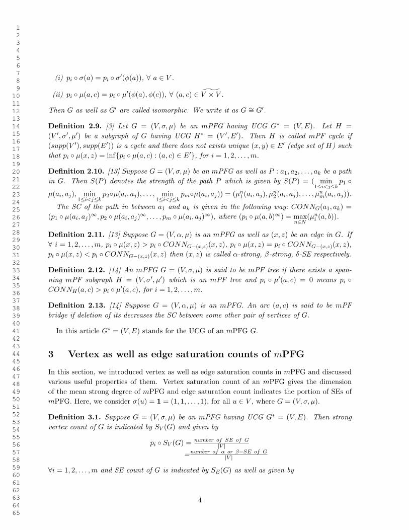
Example 1. Here, we consider an 3PFG to depicted the above definitions. Here, we consider

σ(x) = (1, 1, 1), for all x 2 V .

Figure 1: 3PFG G

Here, the classified edges are given in tabular form.

Edge Classification

(a, b) β-strong

(b, c) α-strong

(a, d) β-strong

(b, d) α-strong

(a, c) δ-strong

(d, c) δ-strong

5

1

2

3

4

5

6

7

8

9

10

11

12

13

14

15

16

17

18

19

20

21

22

23

24

25

26

27

28

29

30

31

32

33

34

35

36

37

38

39

40

41

42

43

44

45

46

47

48

49

50

51

52

53

54

55

56

57

58

59

60

61

62

63

64

65

α-vertex count of G is

pi � αV (G) =2

4=

1

2, for i = 1, 2, 3

and α-edge count of G is

pi � αE(G) =2

6=

1

3, for i = 1, 2, 3.

β-vertex count of G is

pi � βV (G) =2

4=

1

2, for i = 1, 2, 3

and β-edge count of G is

pi � βE(G) =2

6=

1

3, for i = 1, 2, 3

Strong-vertex count of G is

pi � SV (G) =4

4= 1, , for i = 1, 2, 3

and Strong-edge count of G is

pi � SE(G) =4

6=

2

3, for i = 1, 2, 3.

Since every edges in anmPF tree is α-strong by the Theorem 3.18 of [13] therefore pi�αV (G) =n�1n

and pi �αE(G) = n�1n�1 = 1, where n = total number of vertex in an mPF tree G = (V,σ, µ).

Any other mPFG except the mPF tree, the count of α-strong vertex never exceeds the count

of nodes. For a complete mPFG, all possible edges can be made β-strong by allotting the same

MV to the nodes. Then pi � βV (G) =(n2)

2 and pi � βE(G) =(n2)

(n2)= 1, for i = 1, 2, . . . ,m.

Depending on the above observation, we can say the following:

Proposition 1. Suppose G = (V,σ, µ) is an mPFG where |V | = n. Then

(i) 0 pi � αV (G) n�1n

.

(ii) 0 pi � αE(G) 1.

(iii) 0 pi � βV (G) (n2)

2 .

(iv) 0 pi � βE(G) 1.

(v) 0 pi � SV (G) (n2)

2 .

(vi) 0 pi � SE(G) 1.

for each i = 1, 2, . . . ,m.

6

1

2

3

4

5

6

7

8

9

10

11

12

13

14

15

16

17

18

19

20

21

22

23

24

25

26

27

28

29

30

31

32

33

34

35

36

37

38

39

40

41

42

43

44

45

46

47

48

49

50

51

52

53

54

55

56

57

58

59

60

61

62

63

64

65

Proposition 2. Suppose G = (V,σ, µ) is an mPF tree. Then 0 pi � αV (G) pi � αE(G),

8 i = 1, 2, . . . ,m.

Proof. As G is an mPF tree therefore pi � αV (G) = n�1n

, 8 i = 1, 2, . . . ,m and pi � αE(G) =n�1n�1 = 1, 8 i = 1, 2, . . . ,m. Hence, 0 pi � αV (G) pi � αE(G), 8 i = 1, 2, . . . ,m.

3.1 Vertex and edge counts of some well-known mPFG

In this portion, we talk over saturation counts of mPFG structures like mPF cycles, trees , and

blocks in mPFG. Some necessary parts for these structures are also obtained.

Theorem 3.1. Suppose G = (V,σ, µ) be an mPFG having UCG G⇤ = (V,E) where |V | = n.

Then, the following condition are identical:

(i) G be an mPF tree.

(ii) pi � αV (G) = n�1n

as well as pi � αE(G) = 1, 8 i = 1, 2, . . . ,m.

(iii) n⇥ pi � αV (G) = (n� 1)⇥ pi � αE(G), 8 i = 1, 2, . . . ,m.

Proof. (i) ) (ii) done previously.

(ii) ) (iii)

Suppose that pi � αV (G) = n�1n

and pi � αE(G) = 1, 8 i = 1, 2, . . . ,m.

pi � αV (G) =n� 1

n

) n⇥ pi � αV (G) = (n� 1)

) n⇥ pi � αV (G) = (n� 1)⇥ 1

) n⇥ pi � αV (G) = (n� 1)⇥ pi � αE(G) [As pi � αE(G) = 1]

Hence, n⇥ pi � αV (G) = (n� 1)⇥ pi � αE(G), 8 i = 1, 2, . . . ,m.

(iii) ) (i)

Suppose that n⇥ pi � αV (G) = (n� 1)⇥ pi � αE(G), 8 i = 1, 2, . . . ,m.

Since,

n⇥ pi � αV (G) = (n� 1)⇥ pi � αE(G)

)pi � αV (G)

pi � αE(G)=

(n� 1)

n

)pi � αV (G)

pi � αE(G)=

(n� 1)

n= pi � αV (G)

This shows that pi � αE(G) = 1, for each i = 1, 2, . . . ,m.

Hence, G is connected and acyclic only when all edges are α-strong and therefore, G is a tree.

7

1

2

3

4

5

6

7

8

9

10

11

12

13

14

15

16

17

18

19

20

21

22

23

24

25

26

27

28

29

30

31

32

33

34

35

36

37

38

39

40

41

42

43

44

45

46

47

48

49

50

51

52

53

54

55

56

57

58

59

60

61

62

63

64

65

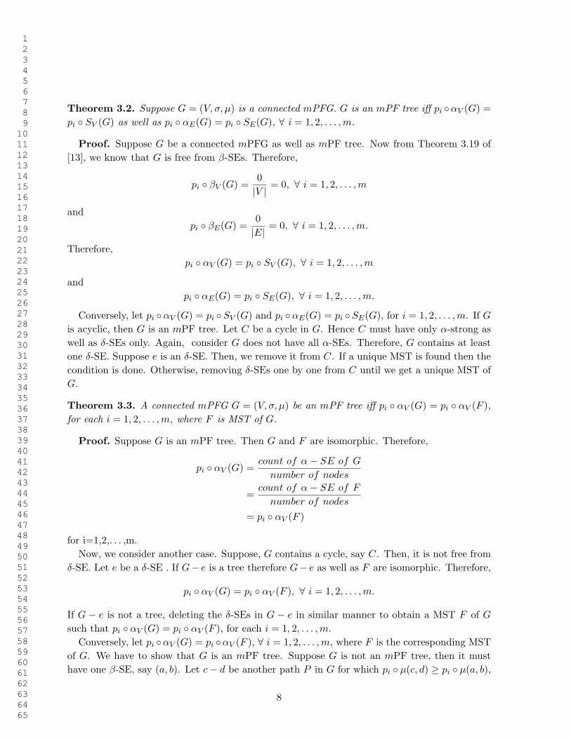
Theorem 3.2. Suppose G = (V,σ, µ) is a connected mPFG. G is an mPF tree iff pi �αV (G) =

pi � SV (G) as well as pi � αE(G) = pi � SE(G), 8 i = 1, 2, . . . ,m.

Proof. Suppose G be a connected mPFG as well as mPF tree. Now from Theorem 3.19 of

[13], we know that G is free from β-SEs. Therefore,

pi � βV (G) =0

|V |= 0, 8 i = 1, 2, . . . ,m

and

pi � βE(G) =0

|E|= 0, 8 i = 1, 2, . . . ,m.

Therefore,

pi � αV (G) = pi � SV (G), 8 i = 1, 2, . . . ,m

and

pi � αE(G) = pi � SE(G), 8 i = 1, 2, . . . ,m.

Conversely, let pi �αV (G) = pi �SV (G) and pi �αE(G) = pi �SE(G), for i = 1, 2, . . . ,m. If G

is acyclic, then G is an mPF tree. Let C be a cycle in G. Hence C must have only α-strong as

well as δ-SEs only. Again, consider G does not have all α-SEs. Therefore, G contains at least

one δ-SE. Suppose e is an δ-SE. Then, we remove it from C. If a unique MST is found then the

condition is done. Otherwise, removing δ-SEs one by one from C until we get a unique MST of

G.

Theorem 3.3. A connected mPFG G = (V,σ, µ) be an mPF tree iff pi � αV (G) = pi � αV (F ),

for each i = 1, 2, . . . ,m, where F is MST of G.

Proof. Suppose G is an mPF tree. Then G and F are isomorphic. Therefore,

pi � αV (G) =count of α� SE of G

number of nodes

=count of α� SE of F

number of nodes

= pi � αV (F )

for i=1,2,. . . ,m.

Now, we consider another case. Suppose, G contains a cycle, say C. Then, it is not free from

δ-SE. Let e be a δ-SE . If G� e is a tree therefore G� e as well as F are isomorphic. Therefore,

pi � αV (G) = pi � αV (F ), 8 i = 1, 2, . . . ,m.

If G � e is not a tree, deleting the δ-SEs in G � e in similar manner to obtain a MST F of G

such that pi � αV (G) = pi � αV (F ), for each i = 1, 2, . . . ,m.

Conversely, let pi �αV (G) = pi �αV (F ), 8 i = 1, 2, . . . ,m, where F is the corresponding MST

of G. We have to show that G is an mPF tree. Suppose G is not an mPF tree, then it must

have one β-SE, say (a, b). Let c� d be another path P in G for which pi � µ(c, d) � pi � µ(a, b),

8

1

2

3

4

5

6

7

8

9

10

11

12

13

14

15

16

17

18

19

20

21

22

23

24

25

26

27

28

29

30

31

32

33

34

35

36

37

38

39

40

41

42

43

44

45

46

47

48

49

50

51

52

53

54

55

56

57

58

59

60

61

62

63

64

65

8 i = 1, 2, . . . ,m and 8 (c, d) 2 P . Now, the join of P as well as (a, b) creates a cycle in G.

Let k be the count of α-SEs which are incident at a. To find F , remove (a, b) from G, which

has minimum weight in C. Then the count of α-SEs connected to c in F is k + 1. Suppose

the remaining counts of α-SEs is k1. Hence, pi � αV (G) = k+1|V | as well as pi � αV (F ) = k+k1+1

|V | ,

8 i = 1, 2, . . . ,m, a contrast. Therefore, the theorem.

4 Saturation in m-polar fuzzy graph

Here, saturation in terms of a node as well as edge counts is presented. In this section, we also

studied some of the interesting facts of it. We also studied saturated blocks in mPFG.

Definition 4.1. Suppose G is an mPFG. Then G is called α-saturate if it must have one α-SEs

incident with each node of G. G is said to be β-strong saturate if it must have one β-SE incident

with each nodes of G.

Definition 4.2. Suppose G is an mPFG. G is called a saturate graph if at least one α-SE as

well as β-SEs incident with every vertex of G. Otherwise G is called an unsaturated mPFG.

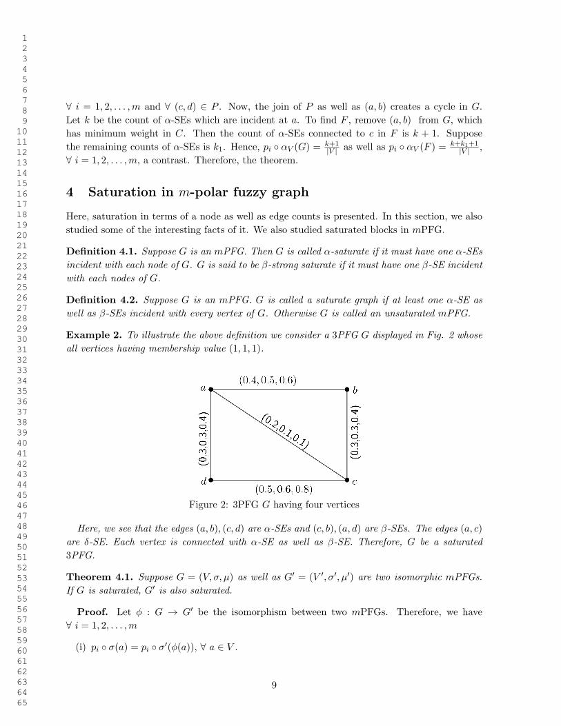
Example 2. To illustrate the above definition we consider a 3PFG G displayed in Fig. 2 whose

all vertices having membership value (1, 1, 1).

Figure 2: 3PFG G having four vertices

Here, we see that the edges (a, b), (c, d) are α-SEs and (c, b), (a, d) are β-SEs. The edges (a, c)

are δ-SE. Each vertex is connected with α-SE as well as β-SE. Therefore, G be a saturated

3PFG.

Theorem 4.1. Suppose G = (V,σ, µ) as well as G0 = (V 0,σ0, µ0) are two isomorphic mPFGs.

If G is saturated, G0 is also saturated.

Proof. Let φ : G ! G0 be the isomorphism between two mPFGs. Therefore, we have

8 i = 1, 2, . . . ,m

(i) pi � σ(a) = pi � σ0(φ(a)), 8 a 2 V .

9

1

2

3

4

5

6

7

8

9

10

11

12

13

14

15

16

17

18

19

20

21

22

23

24

25

26

27

28

29

30

31

32

33

34

35

36

37

38

39

40

41

42

43

44

45

46

47

48

49

50

51

52

53

54

55

56

57

58

59

60

61

62

63

64

65

(ii) pi � µ(a, c) = pi � µ0(φ(a),φ(c)), 8 (a, c) 2 V̂ ⇥ V .

To show G0 is saturated, we have to show that each node is connected with at least one α-SE

as well as β-SEs. Let w0 2 V 0. Then there must be a node, say w, in G for which φ(w) = w0.

Since G is saturated, therefore w is an incident with at least one α-SEs as well as β-SEs. Since,

G and G0 are isomorphic to each other. Therefore, w0 is also incident to at least one α-SEs and

β-SEs. Hence, G0 is also saturated.

Let G be an mPFG having UCG G⇤ = (V,E) where |V | = k. We define a finite sequence

αS(G) = (n1, n2, . . . , nk) called α-strong sequence where, nj = count of α-SEs connect at node

vj . We define a finite sequence βS(G) = (n1, n2, . . . , nk) called β-strong sequence where, nj =

count of β-SEs connect at node vj . Since, the count of SEs of G = (the count of α-SEs of G +

the count of β-SEs of G) therefore,

X

nj2αS(G)

nj +X

nj2βS(G)

nj =X

nj2SS(G)

nj

.

Theorem 4.2. Suppose G = (V,σ, µ) is an mPFG having UCG G⇤ = (V,E) where |V | = k.

Then G is α-saturated iffX

nj2αS(G)

nj � k.

Proof. Suppose G be an α-saturated mPFG. Therefore, at least one α-SEs incident with

each vertex of G. ThusX

nj2αS(G)

nj � 1 + 1 + . . .+ 1

)X

nj2αS(G)

nj � k

Conversely, letX

nj2αS(G)

nj � k. Then, all k nodes of G are connected with at least one α-SEs.

Therefore, G is α-saturated mPFG.

Theorem 4.3. Suppose G = (V,σ, µ) is an mPFG having UCG G⇤ = (V,E) where |V | = k.

Then G is β-saturated iffX

nj2βS(G)

nj � k.

Proof. Similar to the above theorem.

Theorem 4.4. Suppose G = (V,σ, µ) is an mPFG having UCG G⇤ = (V,E) where |V | = k. If

G is β-saturated thenX

nj2SS(G)

nj � 2k.

Proof. Let G be saturated. Therefore, each node of G is connected with at least one α-SE

as well as one β-SE. Thus,X

nj2SS(G)

nj � 2k.

10

1

2

3

4

5

6

7

8

9

10

11

12

13

14

15

16

17

18

19

20

21

22

23

24

25

26

27

28

29

30

31

32

33

34

35

36

37

38

39

40

41

42

43

44

45

46

47

48

49

50

51

52

53

54

55

56

57

58

59

60

61

62

63

64

65

Theorem 4.5. Suppose G = (V,σ, µ) is an mPFG having UCG G⇤ = (V,E) where |V | = n. If,

(i) pi � αV (G) � 0.5 if α-saturated.

(ii) pi � βV (G) � 0.5 if β-saturated.

(iii) pi � SV (G) � 1 if saturated.

8 i = 1, 2, . . . ,m.

Proof. i) Let G is α-saturated then every vertex of G is incident with at least one α-SEs.

Therefore, G must have n2 , α-SEs. Therefore, pi � αV (G) �

n2

n= 0.5.

ii) Similar to the above.

iii) Let G be saturated. Therefore, each node of G is connected with at least one α-SE as

well as β-SEs. Since, the count of SEs of G = (the count of α-SEs of G + the count of β-SEs of

G)� n2 + n

2 = n. Hence, pi � SV (G) � nn= 1.

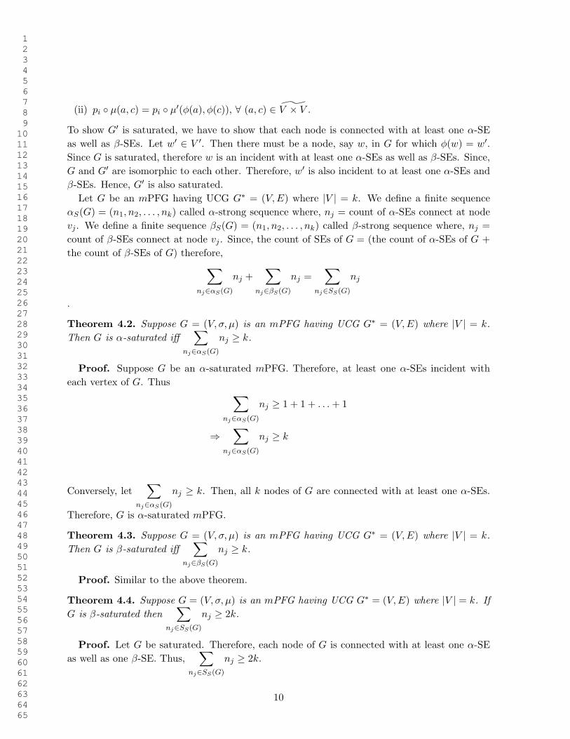
Figure 3: 3PFG G having even number of vertices

In the Fig. 3, all the vertices have membership value (1, 1, 1), that is σ(aj) = (1, 1, 1), for j =

1, 2, . . . , 12. The edges membership value is µ(aj , ak) = (0.6, 0.6, 0.6), where 1 j < k 12

and j is odd and k is even. The edges membership value is µ(aj , ak) = (0.4, 0.4, 0.4), where

1 < j < k < 12 and j is even and k is odd. The edge membership value between a1 and a12 is

(0.4, 0.4, 0.4).

In the Fig. 3, we see that all the edges having membership value (0.6, 0.6, 0.6) are α-strong and

the edges having membership value (0.4, 0.4, 0.4) are β-strong. Therefore, Fig. 3 is saturated.

11

1

2

3

4

5

6

7

8

9

10

11

12

13

14

15

16

17

18

19

20

21

22

23

24

25

26

27

28

29

30

31

32

33

34

35

36

37

38

39

40

41

42

43

44

45

46

47

48

49

50

51

52

53

54

55

56

57

58

59

60

61

62

63

64

65

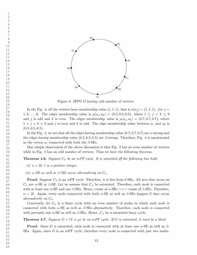
Figure 4: 3PFG G having odd number of vertices

In the Fig. 4, all the vertices have membership value (1, 1, 1), that is σ(aj) = (1, 1, 1), for j =

1, 2, . . . , 9. The edges membership value is µ(aj , ak) = (0.5, 0.5, 0.5), where 1 j < k 9

and j is odd and k is even. The edges membership value is µ(aj , ak) = (0.7, 0.7, 0.7), where

1 < j < k < 9 and j is even and k is odd. The edge membership value between a1 and a9 is

(0.5, 0.5, 0.5).

In the Fig. 4, we see that all the edges having membership value (0.7, 0.7, 0.7) are α-strong and

the edges having membership value (0.5, 0.5, 0.5) are β-strong. Therefore, Fig. 4 is unsaturated

as the vertex a1 connected with both the β-SEs.

One simple observation of the above discussion is that Fig. 3 has an even number of vertices

while in Fig. 4 has an odd number of vertices. Thus we have the following theorem.

Theorem 4.6. Suppose Cn be an mPF cycle. It is saturated iff the following two hold:

(i) n = 2t, t is a positive integer.

(ii) α-SE as well as β-SEs occur alternatively on Cn.

Proof. Suppose Cn is an mPF cycle. Therefore, it is free from δ-SEs. All arcs that occur on

Cn are α-SE or β-SE. Let us assume that Cn be saturated. Therefore, each node is connected

with at least one α-SE and one β-SEs. Hence, count of α-SEs = t = count of β-SEs. Therefore,

n = 2t. Again, every node connected with both α-SE as well as β-SEs happen if they occur

alternatively on Cn.

Conversely, let Cn is a fuzzy cycle with an even number of nodes in which each node is

connected with both α-SE as well as β-SEs alternatively. Therefore, each node is connected

with precisely one α-SE as well as β-SEs. Hence, Cn be a saturated fuzzy cycle.

Theorem 4.7. Suppose G = (V,σ, µ) be an mPF cycle. If G is saturated, it must be a block.

Proof. Since G is saturated, each node is connected with at least one α-SE as well as β-

SEs. Again, since G is an mPF cycle; therefore every node is connected with just two nodes.

12

1

2

3

4

5

6

7

8

9

10

11

12

13

14

15

16

17

18

19

20

21

22

23

24

25

26

27

28

29

30

31

32

33

34

35

36

37

38

39

40

41

42

43

44

45

46

47

48

49

50

51

52

53

54

55

56

57

58

59

60

61

62

63

64

65

Therefore, every node is incident with precisely one α-SE and β-SEs. Hence, removing any node

from G may not decrease SC between other nodes. This shows that G is free from the mPF cut

node; therefore, G is a block.

Theorem 4.8. Let G = (V,σ, µ) is mPF cycle. If G be an mPF blocks, then it is either saturated

or β-saturated.

Proof. Let a block be G. We demand that G is free from δ-SEs. If possible, let e be a δ-SE.

Then the remaining edges must be α-SE, and therefore G contains n � 2 fuzzy cut nodes, an

irrelevance. So, G has no δ-SEs. Thus, G is free from δ-SEs.

If G has only α-SE as well as β-SEs, they appear alternatively; else, the block shape will not

be found. If count of α-SE = count of β-SEs =n2 , then G be α-saturated as well as β-saturated

and therefore it is saturated. If the count of α-SEs is less than the count of β-SEs, then G must

be only β-saturated. For another case, when the count of α-SEs is greater than the count of

β-SEs, it will not be true as it does not form a block. If every arc is β-strong of G, it must be

β-saturated. Therefore, the theorem.

Theorem 4.9. A complete mPFG has no δ-arcs.

Proof. Suppose G = (V,σ, µ) is a complete mPFG. Let G has a δ-arcs. Let (p, q) be the

δ-arcs. Then we have,

pi � µ(p, q) < pi � CONNG�(p,q)µ(p, q), 8 i = 1, 2, . . . ,m.

A stronger path P except the arc (p, q) in G must exist there. Suppose pi � µ(p, q) = ti,

i = 1, 2, . . . ,m and the strength of P be (u1, u2, . . . , um). Therefore, we have ti < ui, 8 i =

1, 2, . . . ,m. Suppose r be the first vertex after u in the path P . Then, we have

pi � µ(p, r) > ti, 8 i = 1, 2, . . . ,m (1)

In a similar way, let s is the last vertex before q in the path P . Again, we also have

pi � µ(s, q) > ti, 8 i = 1, 2, . . . ,m (2)

Since, G be complete mPFG, therefore we have pi � µ(p, q) = min{pi � σ(p), pi � σ(q)}, 8 i =

1, 2, . . . ,m as well as 8 (p, q) 2 E. Therefore, at least one of pi � σ(p) or pi � σ(q) be ti,

8 i = 1, 2, . . . ,m.

Therefore, (1) will contradict if pi � σ(p) = ti, 8 i = 1, 2, . . . ,m and (2) will contradict if

pi � σ(q) = ti, for i = 1, 2, . . . ,m.

Hence, the theorem.

Theorem 4.10. Suppose G = (V,σ, µ) is an mPFG. An arc (a, c) be an mPF bridge iff it is

α-strong.

Proof. Suppose (a, c) be an mPF bridge. Then we have from the definition of mPF bridge,

pi�CONNG�(a,c)(a, c) < pi�CONNG(a, c), for i = 1, 2, . . . ,m (1)

13

1

2

3

4

5

6

7

8

9

10

11

12

13

14

15

16

17

18

19

20

21

22

23

24

25

26

27

28

29

30

31

32

33

34

35

36

37

38

39

40

41

42

43

44

45

46

47

48

49

50

51

52

53

54

55

56

57

58

59

60

61

62

63

64

65

Again, from Theorem 3.11 of [13],

we have pi�µ(a, c) = pi�CONNG(a, c), 8 i = 1, 2, . . . ,m (2)

From (1) and (2), we get pi � µ(a, c) > pi � CONNG�(a,c)(a, c), 8 i = 1, 2, . . . ,m. Hence, (a, c)

be α-SE.

Conversely, suppose (a, c) is an α-SE. Then, we have (a, c) is the one and only one strongest

path in between a and c and removal of (a, c) will decrease the SC of a and b. Therefore, (a, c)

is a bridge.

Theorem 4.11. A complete mPFG has at most one α-SEs.

Proof. We know that complete mPFG have at most one mPF bridge. Again, from Theorem

4.10, we have an arc (a, b) be an mPF bridge iff it is α-SE. Hence, a complete mPFG has at

most one α-SEs.

Proposition 3. Every complete mPFG has at most�n2

�or

�n2

�-1 β-SEs.

Theorem 4.12. If G is a complete mPFG having n vertices, the following inequalities hold.

(i) 0 pi � αV (G) 1n.

(ii) n2�n�22n pi � βV (G) n�1

2 .

8 i = 1, 2, . . . ,m.

Proof. With the help of Theorem 4.11, we have G have at most one α-SEs. Hence, we have

pi � αV (G) 1n, for each i = 1, 2, . . . ,m. Again, clearly pi � αV (G) � 0, for each i = 1, 2, . . . ,m.

Therefore, 0 pi � αV (G) 1n, for each i = 1, 2, . . . ,m.

Again, from Proposition 3, we know that the minimum number of β-SEs are�n2

�-1. Therefore,

pi � βV (G) �n(n�1

2 )� 1

n

�n2 � n� 2

2n

Thus, n2�n�22n pi � βV (G) n�1

2 , for each i = 1, 2, . . . ,m.

Next, we will try to find out the upper limit of α-node count for a block in mPFG.

Theorem 4.13. If G = (V,σ, µ) is an mPF blocks, we have pi �αV (G) 0.5, 8 i = 1, 2, . . . ,m.

Proof. To prove this, we first try to find out the maximum count of α-SEs of G. Let |V | = n.

We know that if more than one α-SEs are connected with a common node then the node is a

mPF cut node. Since, G is an mPF block, therefore it has no mPF cut node. Therefore, the

maximum count of α-SEs of G is n2 . Thus, pi � αV (G)

n2

n= 0.5, 8 i = 1, 2, . . . ,m.

Theorem 4.14. An mPF block G be α-saturated then pi � αV (G) = 0.5, 8 i = 1, 2, . . . ,m.

Proof. Let G be α-saturated. Since, G is an mPF block, therefore it has no mPF cut vertex.

Hence, every vertex incident with exactly unique α-SE. Therefore, G contains exactly n2 count

of α-SEs. Thus, pi � αV (G) =n2

n= 0.5, for i = 1, 2, . . . ,m.

14

1

2

3

4

5

6

7

8

9

10

11

12

13

14

15

16

17

18

19

20

21

22

23

24

25

26

27

28

29

30

31

32

33

34

35

36

37

38

39

40

41

42

43

44

45

46

47

48

49

50

51

52

53

54

55

56

57

58

59

60

61

62

63

64

65

5 Algorithms

From Dijkstra’s algorithm [5], we first trace G⇤ = (V,E), where V as well as E indicates the set

of all nodes as well edges where |V | = n.

Algorithm 1 An algorithm to find α-saturation in mPFG

Input: A mPFG G = (V,σ, µ).

Output: Finding α-saturated mPFG.

Step 1: Put the membership value of vertices aj , j = 1, 2, . . . , n .

Step 2: Put the membership value of edges which satisfied pi � µ(aj , ak) inf{pi � σ(aj), pi �

σ(ak)}, i = 1, 2, . . . ,m.

Step 3: Calculate pi � CONNG�((aj ,ak))(aj , ak), for i = 1, 2, . . . ,m, 8(aj , ak) 2 E.

Step 4: Verify pi � µ(aj , ak) > pi � CONNG�(aj ,ak)(aj , ak), 8(aj , ak) 2 E.

Step 5: Select all α-SEs in G.

Step 6: Check whether every node is connected with at least one α-SEs or not.

Algorithm 2 An algorithm to find β-saturation in mPFG

Input: A mPFG G = (V,σ, µ).

Output: Finding β-saturated mPFG.

Step 1: Put the membership value of vertices aj , j = 1, 2, . . . , n .

Step 2: Put the membership value of edges which satisfied pi � µ(aj , ak) inf{pi � σ(aj), pi �

σ(ak)}, i = 1, 2, . . . ,m.

Step 3: Calculate pi � CONNG�((aj ,ak))(aj , ak), for i = 1, 2, . . . ,m, 8(aj , ak) 2 E.

Step 4: Verify pi � µ(aj , ak) = pi � CONNG�(aj ,ak)(aj , ak), 8(aj , ak) 2 E.

Step 5: Select all β-SEs in G.

Step 6: Check whether every node is connected with at least one β-SEs or not.

Algorithm 3 An algorithm to find saturation in mPFG

Input: A mPFG G = (V,σ, µ).

Output: Finding saturated mPFG.

Step 1: Put the membership value of vertices aj , j = 1, 2, . . . , n .

Step 2: Put the membership value of edges which satisfied pi � µ(aj , ak) inf{pi � σ(aj), pi �

σ(ak)}, i = 1, 2, . . . ,m.

Step 3: Using Algorithms 1 and 2 identified all α-strong as well as β-SEs in G.

Step 4: Check whether every vertex is connected with at least one α-SEs as well as β-SEs or

not.

15

1

2

3

4

5

6

7

8

9

10

11

12

13

14

15

16

17

18

19

20

21

22

23

24

25

26

27

28

29

30

31

32

33

34

35

36

37

38

39

40

41

42

43

44

45

46

47

48

49

50

51

52

53

54

55

56

57

58

59

60

61

62

63

64

65

6 Application

The mPFG is an essential mathematical structure representing the facts in real-life connected

through graphical systems, in which nodes and edges lie in an m-polar fuzzy information. In

this section, by using saturation in mPFG, we solve one particular allocation problem.

6.1 Model construction

In modern days, education is an essential topic for every person. Under the rule of the Right to

Education (RTE) in 2005, everybody has the opportunity to read and write. In the education

system, IIT(Indian Institute of Technology) is one of the most important institutions for higher

studies in India. Therefore, establishing an IIT in a town among some towns is not an easy task

for any Government.

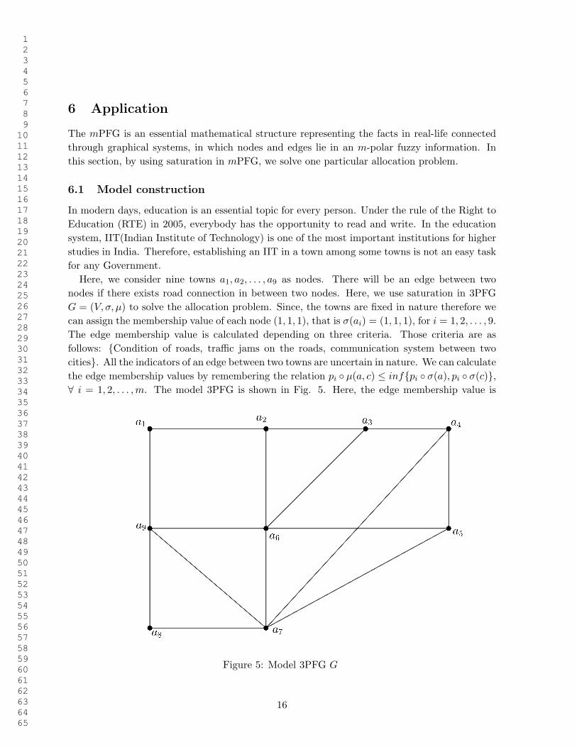
Here, we consider nine towns a1, a2, . . . , a9 as nodes. There will be an edge between two

nodes if there exists road connection in between two nodes. Here, we use saturation in 3PFG

G = (V,σ, µ) to solve the allocation problem. Since, the towns are fixed in nature therefore we

can assign the membership value of each node (1, 1, 1), that is σ(ai) = (1, 1, 1), for i = 1, 2, . . . , 9.

The edge membership value is calculated depending on three criteria. Those criteria are as

follows: {Condition of roads, traffic jams on the roads, communication system between two

cities}. All the indicators of an edge between two towns are uncertain in nature. We can calculate

the edge membership values by remembering the relation pi � µ(a, c) inf{pi � σ(a), pi � σ(c)},

8 i = 1, 2, . . . ,m. The model 3PFG is shown in Fig. 5. Here, the edge membership value is

Figure 5: Model 3PFG G

16

1

2

3

4

5

6

7

8

9

10

11

12

13

14

15

16

17

18

19

20

21

22

23

24

25

26

27

28

29

30

31

32

33

34

35

36

37

38

39

40

41

42

43

44

45

46

47

48

49

50

51

52

53

54

55

56

57

58

59

60

61

62

63

64

65

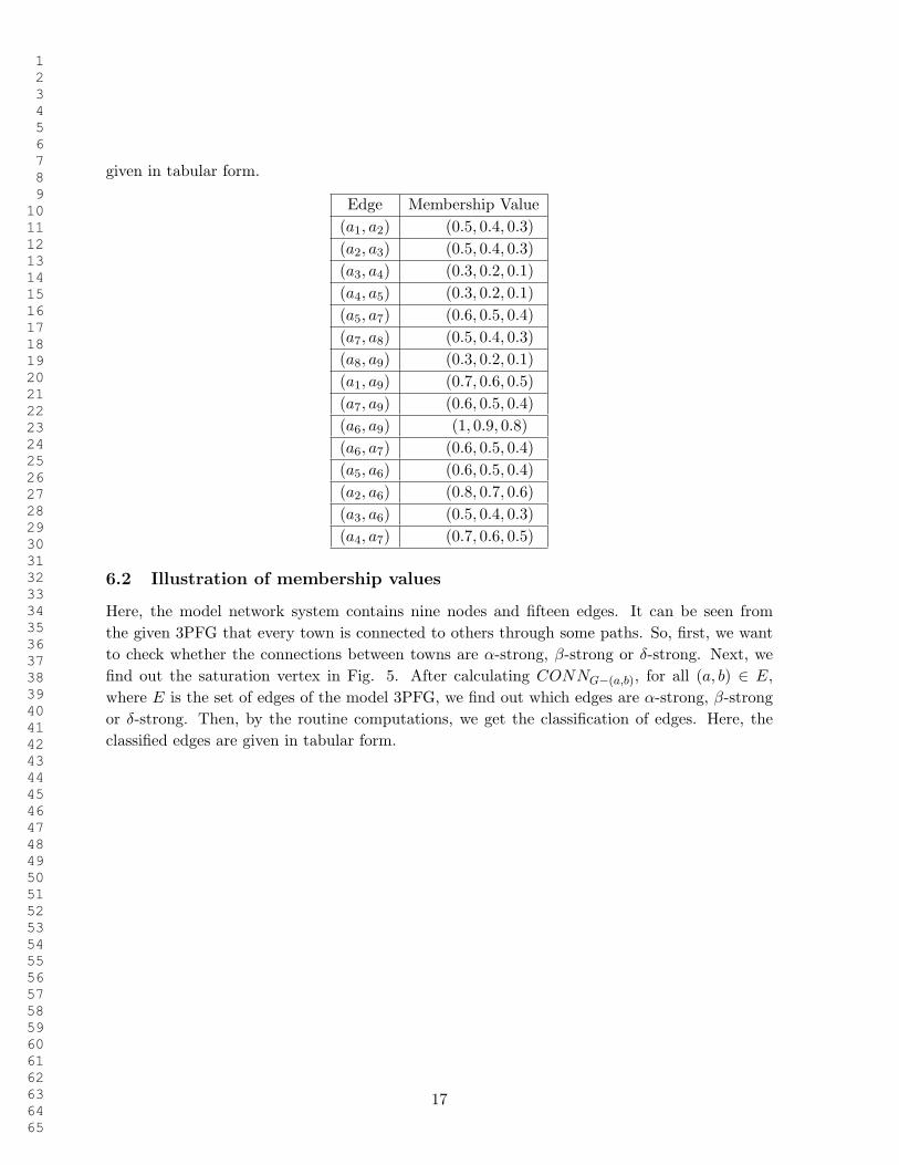
given in tabular form.

Edge Membership Value

(a1, a2) (0.5, 0.4, 0.3)

(a2, a3) (0.5, 0.4, 0.3)

(a3, a4) (0.3, 0.2, 0.1)

(a4, a5) (0.3, 0.2, 0.1)

(a5, a7) (0.6, 0.5, 0.4)

(a7, a8) (0.5, 0.4, 0.3)

(a8, a9) (0.3, 0.2, 0.1)

(a1, a9) (0.7, 0.6, 0.5)

(a7, a9) (0.6, 0.5, 0.4)

(a6, a9) (1, 0.9, 0.8)

(a6, a7) (0.6, 0.5, 0.4)

(a5, a6) (0.6, 0.5, 0.4)

(a2, a6) (0.8, 0.7, 0.6)

(a3, a6) (0.5, 0.4, 0.3)

(a4, a7) (0.7, 0.6, 0.5)

6.2 Illustration of membership values

Here, the model network system contains nine nodes and fifteen edges. It can be seen from

the given 3PFG that every town is connected to others through some paths. So, first, we want

to check whether the connections between towns are α-strong, β-strong or δ-strong. Next, we

find out the saturation vertex in Fig. 5. After calculating CONNG�(a,b), for all (a, b) 2 E,

where E is the set of edges of the model 3PFG, we find out which edges are α-strong, β-strong

or δ-strong. Then, by the routine computations, we get the classification of edges. Here, the

classified edges are given in tabular form.

17

1

2

3

4

5

6

7

8

9

10

11

12

13

14

15

16

17

18

19

20

21

22

23

24

25

26

27

28

29

30

31

32

33

34

35

36

37

38

39

40

41

42

43

44

45

46

47

48

49

50

51

52

53

54

55

56

57

58

59

60

61

62

63

64

65

Edge Classification

(a1, a2) δ-strong

(a2, a3) δ-strong

(a3, a4) δ-strong

(a4, a5) δ-strong

(a5, a7) δ-strong

(a7, a8) α-strong

(a8, a9) δ-strong

(a1, a9) α-strong

(a7, a9) δ-strong

(a6, a9) α-strong

(a6, a7) δ-strong

(a5, a6) δ-strong

(a2, a6) α-strong

(a3, a6) β-strong

(a4, a7) α-strong

Here, only one β-SEs are present in the model 3PFG G. The node a6 is the only saturation

node in the model 3PFG G as it is an incident with at least one α-SE and one β-SEs.

6.3 Decision making

Since a6 is the only saturation node in the model 3PFG G, we can say that the town a6 is the

most suitable place to establish the IIT (Indian Institute of Technology) among all other towns

considered in this proposed model.

We know that saturation in mPFG plays an essential role in this type of allocation problem

through the above discussion. Moreover, we also recognize that saturation in mPFG is more

applicable than saturation in FG in allocation problems.

7 Conclusion

In this paper, α-saturation as well as β-saturation in mPFG along with its several properties are

initiated. Vertex and edge saturation count in mPFG and a few of its facts on some well known

mPFG is also introduced. The upper and lower bound of a vertex as well as edge saturation

count in mPFG are also investigated. Saturation in mPFG by using α-saturation as well as β-

saturation are also discussed here along with some of its intersecting properties. Using saturation

in mPFG, an application is also given in the last part of this paper. Our research work will be

extended depending on mPFG to find more characteristics and applications.

18

1

2

3

4

5

6

7

8

9

10

11

12

13

14

15

16

17

18

19

20

21

22

23

24

25

26

27

28

29

30

31

32

33

34

35

36

37

38

39

40

41

42

43

44

45

46

47

48

49

50

51

52

53

54

55

56

57

58

59

60

61

62

63

64

65

Compliance with ethical standards

Ethical approval This article does not contain any studies with human participants or animals

performed by any of the authors.

Conflict of interest It has been declared by the authors that no conflict of interest of any

person(s) or organization(s) has happened.

Funding details This research has no funding by any organization or individual.

Informed Consent It was obtained from all individual participants included in the study.

Authors’ contributions

All the authors contribute equally in this work.

References

[1] Akram M and Adeel A (2017) m-polar fuzzy graphs and m-polar fuzzy line graphs. Journal

of Discrete Mathematical Sciences and Cryptography 20(8): 1597-1617.

[2] Akram M, Wassem N and Dudek W A (2016) Certain types of edge m-polar fuzzy graph.

Iranian Journal of Fuzzy System 14(4): 27-50.

[3] Akram M (2019) m-polar fuzzy graphs, theory, methods, application. DOI: 10.1007/978-3-

030-03751-2, Springer International Publishing.

[4] Chen J, Li S, Ma S, and Wang X (2014) m-polar fuzzy sets: an extension of bipolar fuzzy

sets. The Scientific World Journal 2014: 1-8.

[5] Douglas B W (2002) Introduction to graph theory. Pearson Education India, Noida

[6] Ghorai G and Pal M (2015) On some operations and density of m-polar fuzzy graphs.

Pacific Science Review A: Natural Science and Engineering 17(1): 14-22.

[7] Ghorai G and Pal M (2016) Some properties of m-polar fuzzy graphs. Pacific Science

Review A: Natural Science and Engineering 18: 38-46.

[8] Ghorai G and Pal M (2016) A study on m-polar fuzzy planar graphs. International Journal

of Computing Science and Mathematics 7(3): 283-292.

[9] Ghorai G and Pal M (2016) Faces and dual of m-polar fuzzy planar graphs. Journal of

Intelligent and Fuzzy Systems 31: 2043-2049.

[10] Kauffman A (1973) Introduction a la Theorie des Sous-emsembles Flous, Mansson et Cie

1: 1973.

[11] Mahapatra T and Pal M (2018) Fuzzy colouring of m-polar fuzzy graph and its application.

Journal of Intelligent and Fuzzy Systems 35(6): 6379-6391.

19

1

2

3

4

5

6

7

8

9

10

11

12

13

14

15

16

17

18

19

20

21

22

23

24

25

26

27

28

29

30

31

32

33

34

35

36

37

38

39

40

41

42

43

44

45

46

47

48

49

50

51

52

53

54

55

56

57

58

59

60

61

62

63

64

65

[12] Mahapatra T, Ghorai G and Pal M (2020) Fuzzy fractional coloring on fuzzy

graph with its application. Journal of Ambient Intelligence and Humanized Computing

https://doi.org/10.1007/s12652-020-01953-9.

[13] Mandal S, Sahoo S, Ghorai G and Pal M (2018) Different Types of Arcs in m-polar Fuzzy

Graphs with Application. J. of Mult.Valued Logic and Soft Computing 34: 263-282.

[14] Mandal S, Sahoo S, Ghorai G and Pal M (2018) Application of SEs in m-Polar Fuzzy

Graphs. Neural Processing Letters https://doi.org/10.1007/s11063-018-9934-1.

[15] Mathew S and Sunitha M S (2012) Fuzzy graphs: basics, concepts and applications. Lap

Lambert Academic Publishing.

[16] Mathew S, Yang L H and Mathew K J (2018) Saturation in Fuzzy Graphs New Mathematics

and Natural Computation 14(1): 113-128.

[17] Mordeson J N and Nair P S (2000) Fuzzy graph and fuzzy hypergraphs. Physica-Verlag

Heidelberg.

[18] Nair P S and Cheng S C (2001) Cliques and fuzzy cliques in fuzzy graphs. IFSA World

Congress and 20th NAFIPS International Conference 4: 2277-2280.

[19] Pal M, Samanta S, Ghorai G (2020) Modern Trends in Fuzzy Graph Theory, Springer.

[20] Rosenfeld A (1975) Fuzzy Graphs, fuzzy sets and their application. Academic Press,New

York. pp. 77-95.

[21] Sunitha S M and Mathew S (2013) Fuzzy graph theory: a survey. Annals of Pure and

Applied Mathematics 4: 92-110.

[22] Zhang R W (1994) Bipolar fuzzy sets and relations:a computational framework for cognitive

modeling and multiagent decision analysis, Proceedings of IEEE Conference 305–309.

[23] Zhang R W (1998) Bipolar fuzzy sets. Proceedings of IEEE Conference 835–840.

[24] Zadeh L A (1965) Fuzzy sets. Information and Control: 338-353.

20

1

2

3

4

5

6

7

8

9

10

11

12

13

14

15

16

17

18

19

20

21

22

23

24

25

26

27

28

29

30

31

32

33

34

35

36

37

38

39

40

41

42

43

44

45

46

47

48

49

50

51

52

53

54

55

56

57

58

59

60

61

62

63

64

65