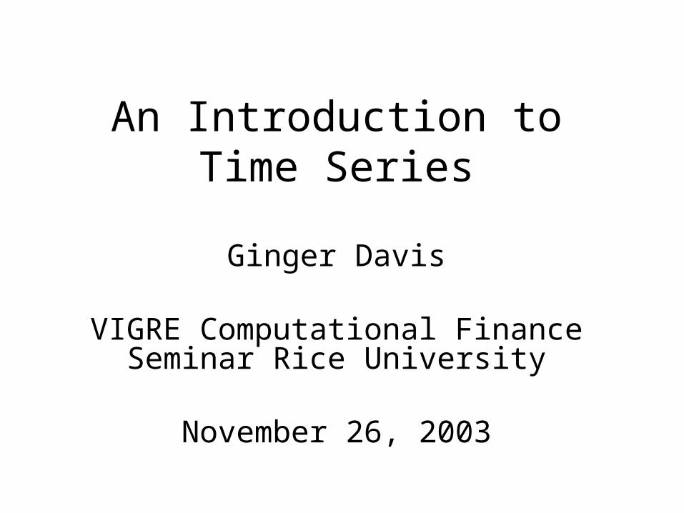
An Introduction to Time Series

Ginger Davis

VIGRE Computational Finance Seminar Rice University

November 26, 2003

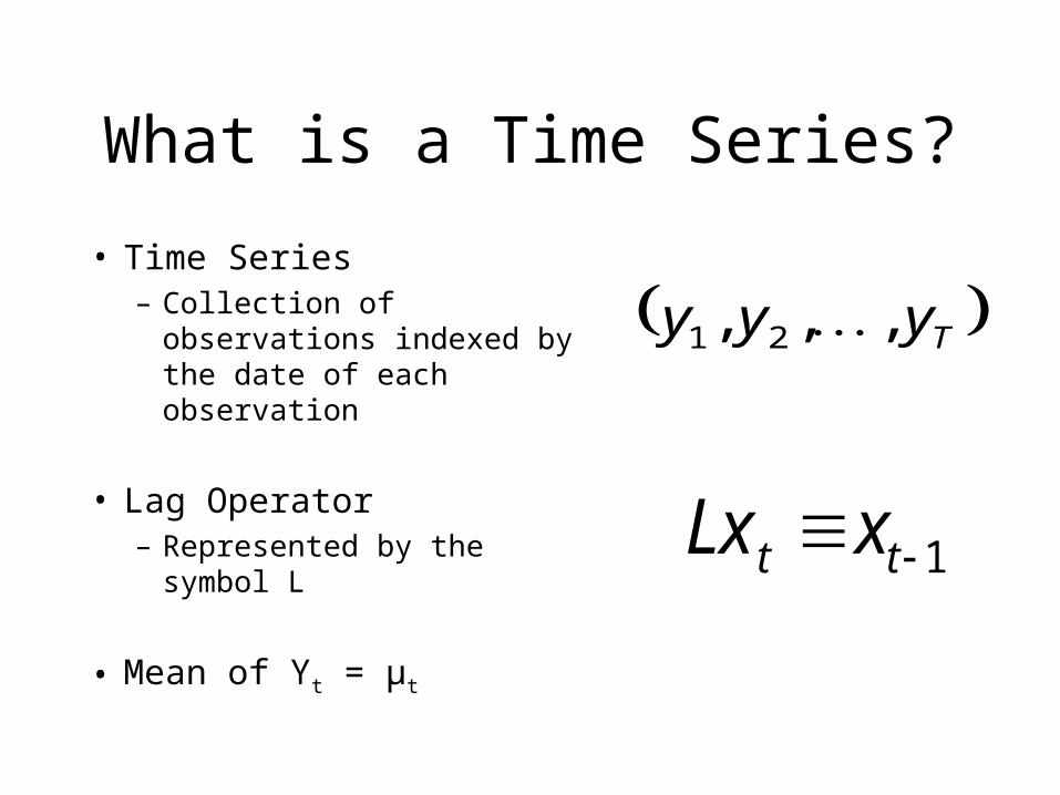
What is a Time Series?

• Time Series– Collection of observations

indexed by the date of each observation

• Lag Operator– Represented by the symbol L

• Mean of Yt = μt

Tyyy ,,, 21

1 tt xLx

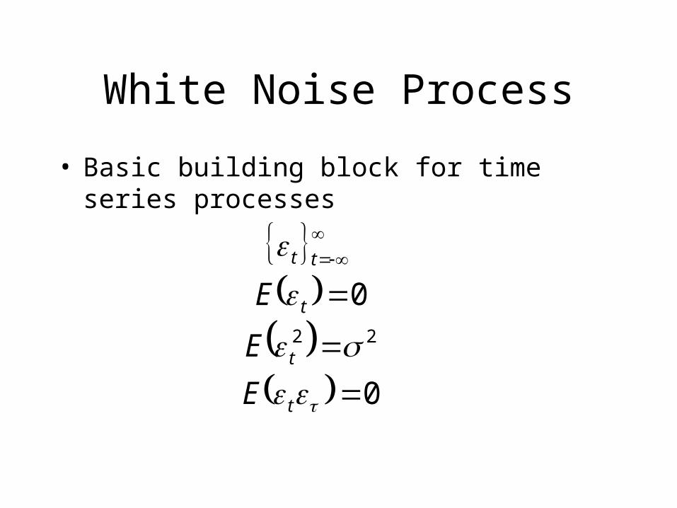
White Noise Process

• Basic building block for time series processes

0

022

t

t

t

tt

E

E

E

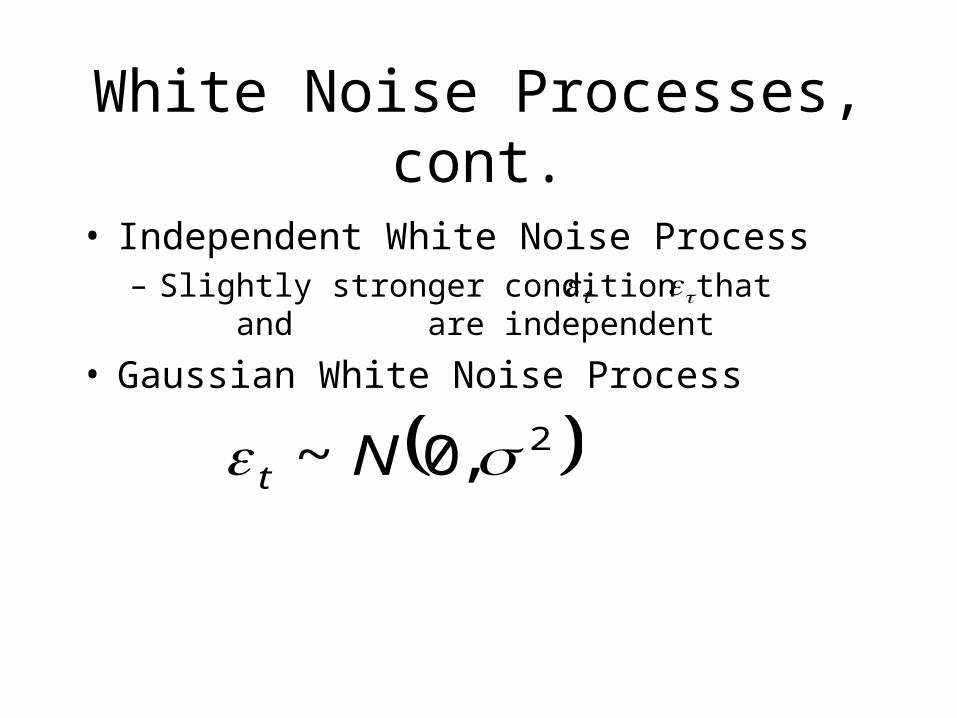
White Noise Processes, cont.

• Independent White Noise Process– Slightly stronger condition that and are

independent

• Gaussian White Noise Process

2,0~ Nt

t

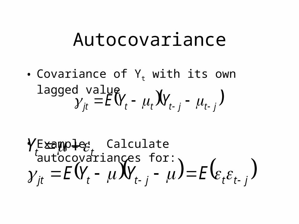
Autocovariance

• Covariance of Yt with its own lagged value

• Example: Calculate autocovariances for:

jtjtttjt YYE

jttjttjt

tt

EYYE

Y

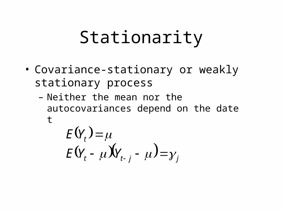
Stationarity

• Covariance-stationary or weakly stationary process– Neither the mean nor the autocovariances depend on

the date t

jjtt

t

YYE

YE

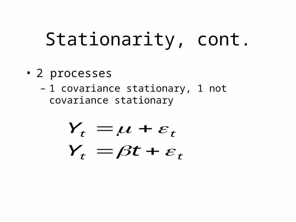
Stationarity, cont.

• 2 processes– 1 covariance stationary, 1 not covariance

stationary

tt

tt

tY

Y

Stationarity, cont.

• Covariance stationary processes– Covariance between Yt and Yt-j depends only on

j (length of time separating the observations) and not on t (date of the observation)

jj

Stationarity, cont.

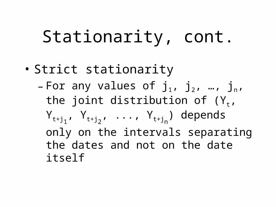
• Strict stationarity– For any values of j1, j2, …, jn, the joint

distribution of (Yt, Yt+j1, Yt+j2

, ..., Yt+jn) depends

only on the intervals separating the dates and not on the date itself

Gaussian Processes

• Gaussian process {Yt}– Joint density

is Gaussian for any

• What can be said about a covariance stationary Gaussian process?

nnjtjt jtjttYYY yyyf

,,,111 ,,,

njjj ,,, 21

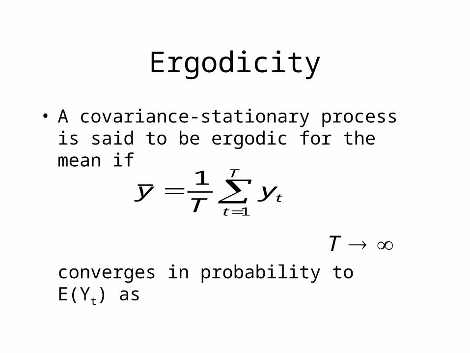
Ergodicity

• A covariance-stationary process is said to be ergodic for the mean if

converges in probability to E(Yt) as

T

tty

Ty

1

1

T

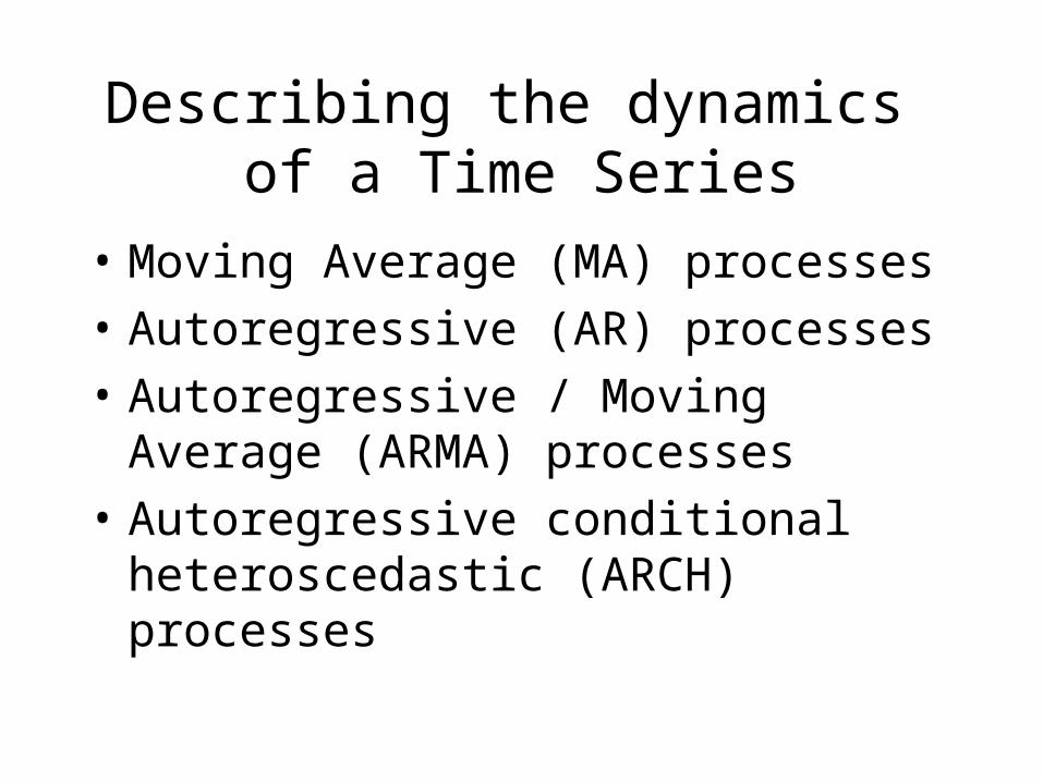
Describing the dynamics of a Time Series

• Moving Average (MA) processes

• Autoregressive (AR) processes

• Autoregressive / Moving Average (ARMA) processes

• Autoregressive conditional heteroscedastic (ARCH) processes

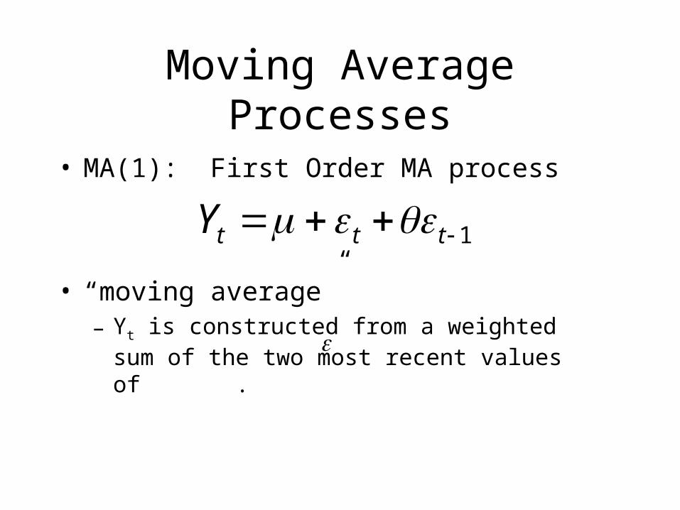
Moving Average Processes

• MA(1): First Order MA process

• “moving average”– Yt is constructed from a weighted sum of the two

most recent values of .

1 tttY

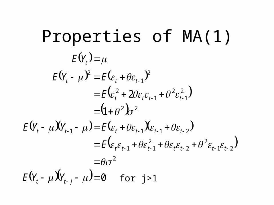
Properties of MA(1)

0

1

2

2

212

22

11

2111

22

21

21

2

21

2

jtt

ttttttt

tttttt

tttt

ttt

t

YYE

E

EYYE

E

EYE

YE

for j>1

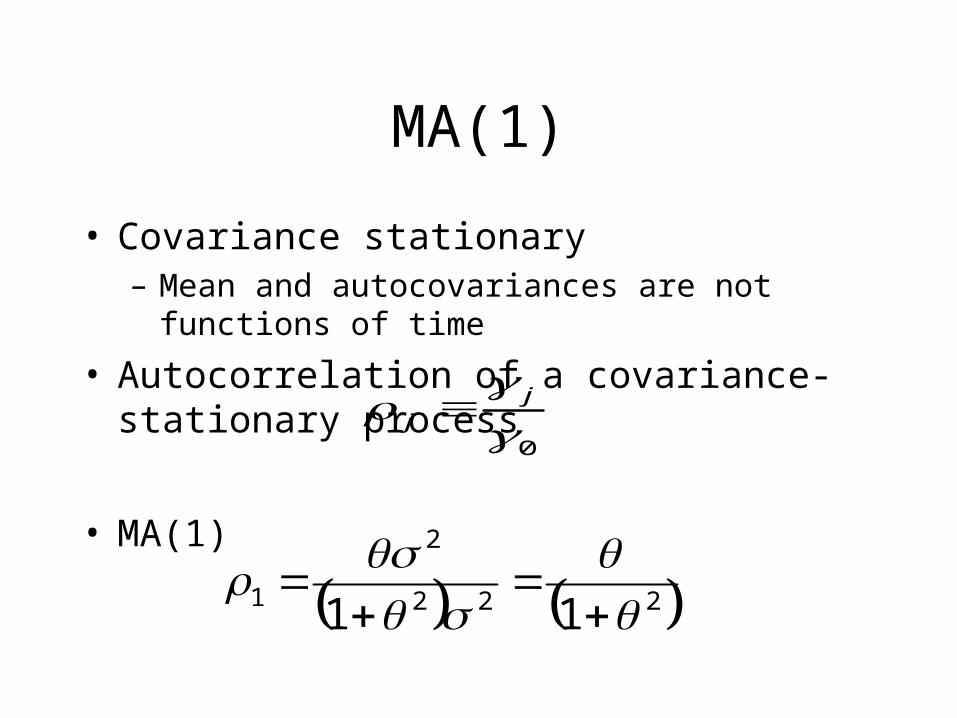
MA(1)

• Covariance stationary– Mean and autocovariances are not functions of time

• Autocorrelation of a covariance-stationary process

• MA(1)0

j

j

222

2

1 11

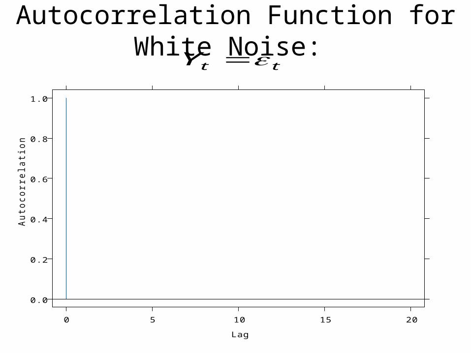
Autocorrelation Function for White Noise:

0.0

0.2

0.4

0.6

0.8

1.0

0 5 10 15 20

Lag

Autocorrelation

ttY

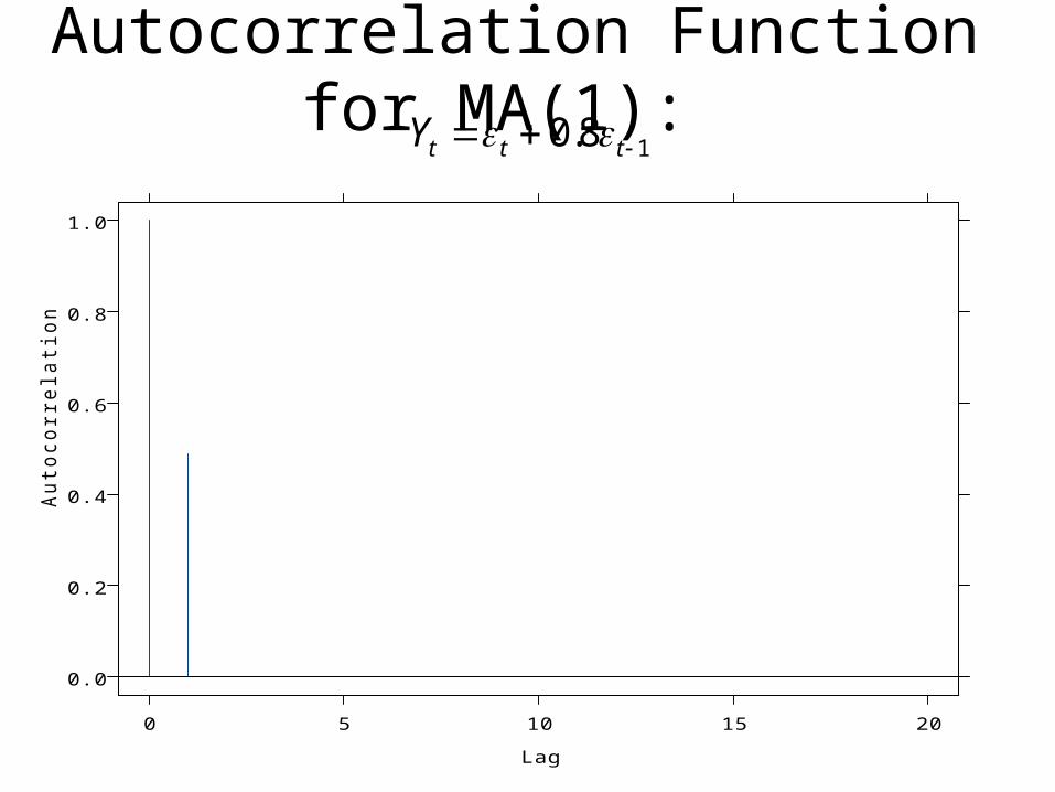
Autocorrelation Function for MA(1): 18.0 tttY

0.0

0.2

0.4

0.6

0.8

1.0

0 5 10 15 20

Lag

Autocorrelation

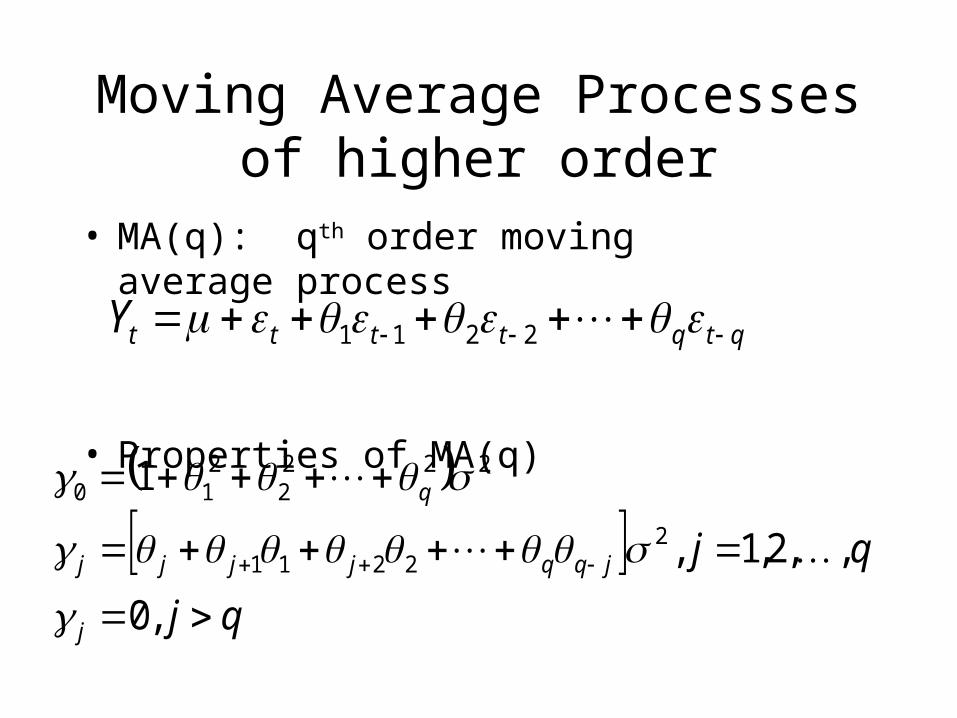
Moving Average Processesof higher order

• MA(q): qth order moving average process

• Properties of MA(q)

qtqttttY 2211

qj

qj

j

jqqjjjj

q

,0

,,2,1,

12

2211

2222

210

Autoregressive Processes

• AR(1): First order autoregression

• Stationarity: We will assume• Can represent as an MA

ttt YcY 1

1

22

1

22

1

1 ttt

tttt

c

cccY

:)(

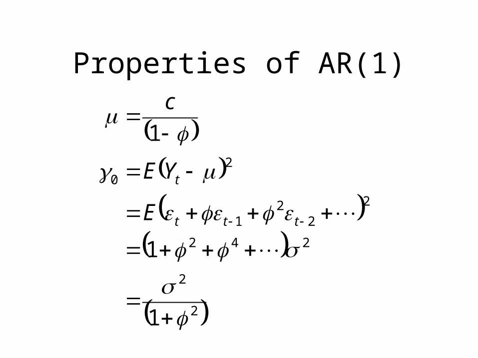
Properties of AR(1)

2

2

242

2

22

1

20

1

1

1

ttt

t

E

YE

c

Properties of AR(1), cont.

jj

j

j

j

jjj

jtjtjtjtj

ttt

jttj

E

YYE

0

22

242

242

22

122

1

1

1

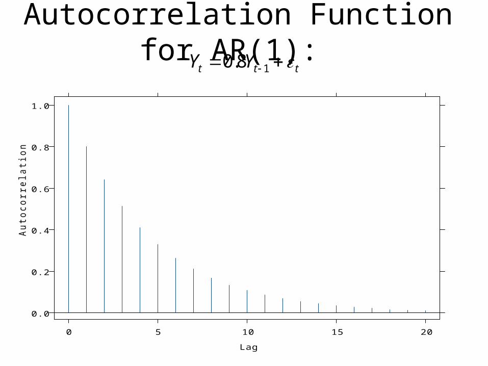
Autocorrelation Function for AR(1): ttt YY 18.0

0.0

0.2

0.4

0.6

0.8

1.0

0 5 10 15 20

Lag

Autocorrelation

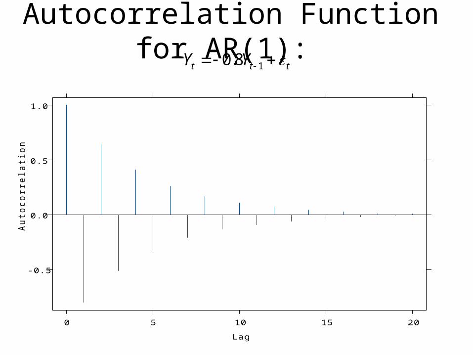
Autocorrelation Function for AR(1): ttt YY 18.0

-0.5

0.0

0.5

1.0

0 5 10 15 20

Lag

Autocorrelation

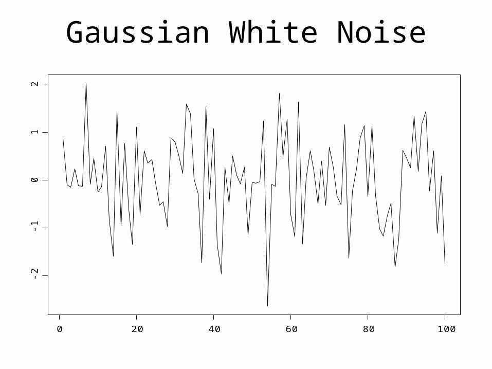
Gaussian White Noise

0 20 40 60 80 100

-2-1

01

2

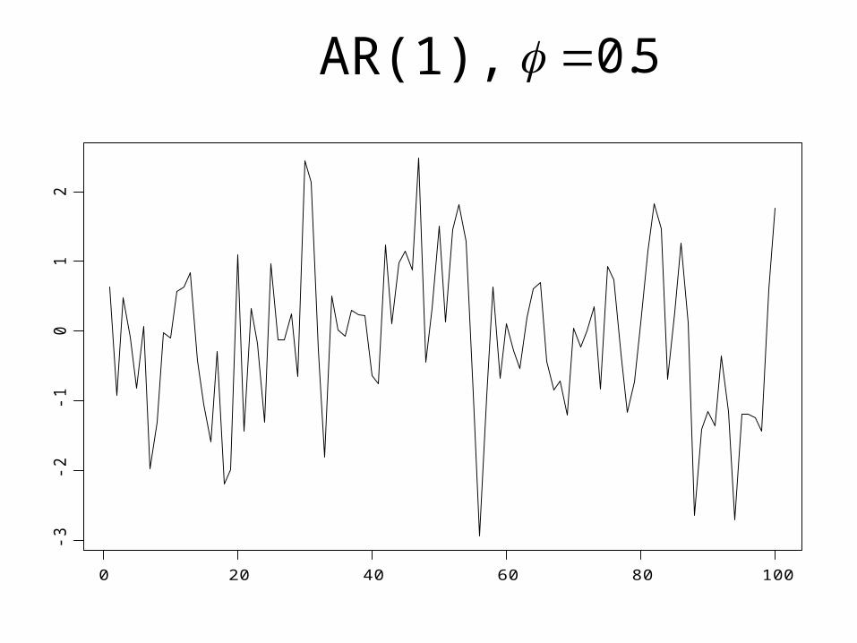
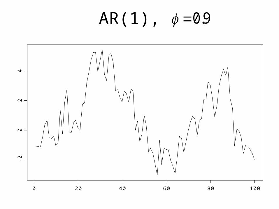
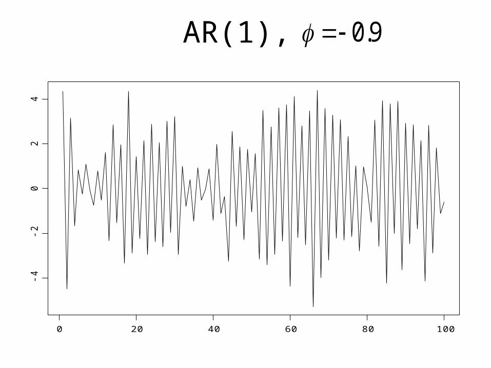
AR(1),

0 20 40 60 80 100

-3-2

-10

12

5.0

AR(1),

0 20 40 60 80 100

-20

24

9.0

AR(1),

0 20 40 60 80 100

-4-2

02

49.0

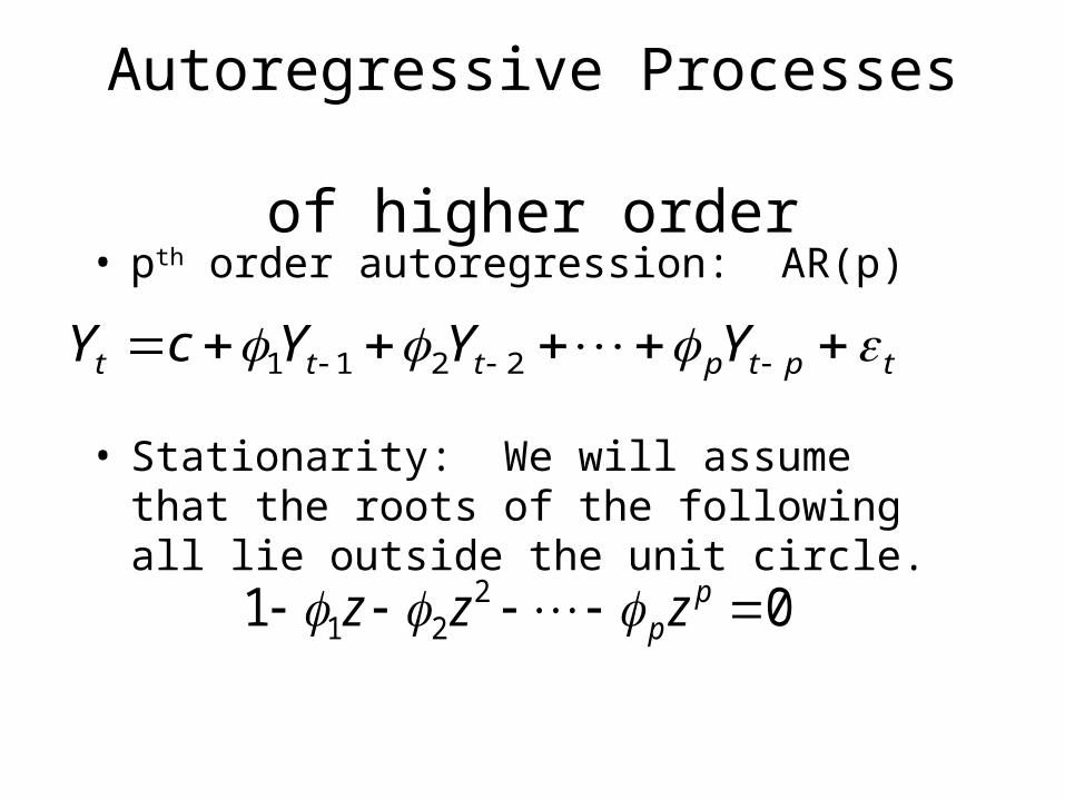
Autoregressive Processes of higher order

• pth order autoregression: AR(p)

• Stationarity: We will assume that the roots of the following all lie outside the unit circle.

tptpttt YYYcY 2211

01 221 p

p zzz

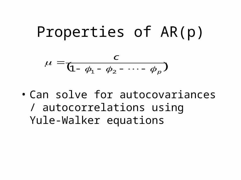
Properties of AR(p)

• Can solve for autocovariances / autocorrelations using Yule-Walker equations

p

c

211

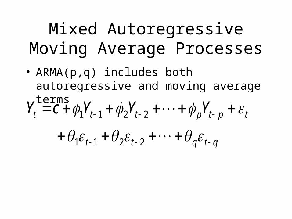
Mixed Autoregressive Moving Average Processes

• ARMA(p,q) includes both autoregressive and moving average terms

qtqtt

tptpttt YYYcY

2211

2211

Time Series Models for Financial Data

• A Motivating Example– Federal Funds rate– We are interested in forecasting not only the

level of the series, but also its variance.– Variance is not constant over time

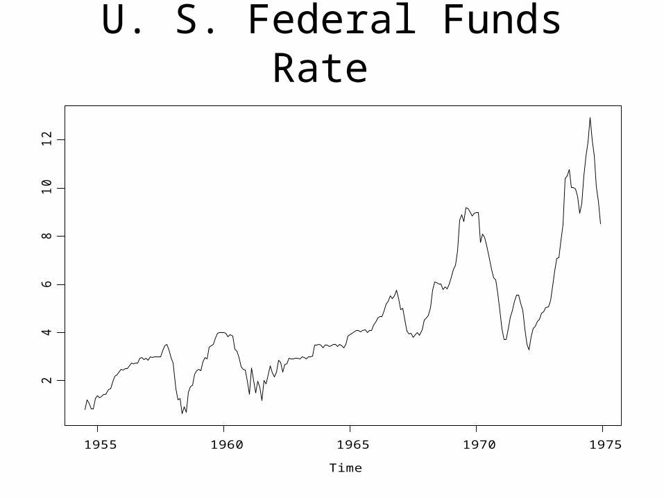
U. S. Federal Funds Rate

Time

1955 1960 1965 1970 1975

24

68

10

12

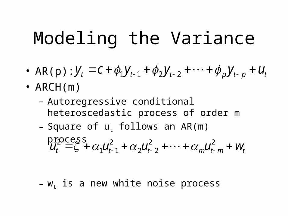
Modeling the Variance

• AR(p):• ARCH(m)

– Autoregressive conditional heteroscedastic process of order m

– Square of ut follows an AR(m) process

– wt is a new white noise process

tptpttt uyyycy 2211

tmtmttt wuuuu 22

222

112

References

• Investopia.com

• Economagic.com

• Hamilton, J. D. (1994), Time Series Analysis, Princeton, New Jersey: Princeton University Press.