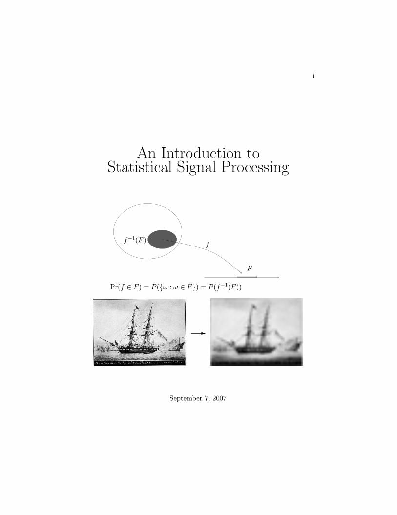
i

An Introduction toStatistical Signal Processing

Pr(f ∈ F ) = P (ω : ω ∈ F) = P (f−1(F ))

f−1(F )f

F

-

September 7, 2007

ii

An Introduction to

Statistical Signal Processing

Robert M. Gray

and

Lee D. Davisson

Information Systems Laboratory

Department of Electrical Engineering

Stanford University

and

Department of Electrical Engineering and Computer Science

University of Maryland

c©2004 by Cambridge University Press. Copies of the pdf file may be

downloaded for individual use, but multiple copies cannot be made or printed

without permission.

iii

to our Families

Contents

Preface page ix

Acknowledgements xii

Glossary xiii

1 Introduction 1

2 Probability 10

2.1 Introduction 10

2.2 Spinning pointers and flipping coins 14

2.3 Probability spaces 22

2.4 Discrete probability spaces 45

2.5 Continuous probability spaces 54

2.6 Independence 69

2.7 Elementary conditional probability 70

2.8 Problems 74

3 Random variables, vectors, and processes 83

3.1 Introduction 83

3.2 Random variables 94

3.3 Distributions of random variables 103

3.4 Random vectors and random processes 113

3.5 Distributions of random vectors 116

3.6 Independent random variables 125

3.7 Conditional distributions 128

3.8 Statistical detection and classification 133

3.9 Additive noise 136

3.10 Binary detection in Gaussian noise 143

3.11 Statistical estimation 145

3.12 Characteristic functions 146

3.13 Gaussian random vectors 152

3.14 Simple random processes 153

v

vi Contents

3.15 Directly given random processes 157

3.16 Discrete time Markov processes 159

3.17 ⋆Nonelementary conditional probability 168

3.18 Problems 169

4 Expectation and averages 183

4.1 Averages 183

4.2 Expectation 186

4.3 Functions of random variables 189

4.4 Functions of several random variables 196

4.5 Properties of expectation 196

4.6 Examples 198

4.7 Conditional expectation 207

4.8 ⋆Jointly Gaussian vectors 210

4.9 Expectation as estimation 212

4.10 ⋆Implications for linear estimation 219

4.11 Correlation and linear estimation 222

4.12 Correlation and covariance functions 229

4.13 ⋆The central limit theorem 232

4.14 Sample averages 235

4.15 Convergence of random variables 237

4.16 Weak law of large numbers 244

4.17 ⋆Strong law of large numbers 246

4.18 Stationarity 250

4.19 Asymptotically uncorrelated processes 256

4.20 Problems 259

5 Second-order theory 276

5.1 Linear filtering of random processes 277

5.2 Linear systems I/O relations 279

5.3 Power spectral densities 285

5.4 Linearly filtered uncorrelated processes 287

5.5 Linear modulation 294

5.6 White noise 297

5.7 ⋆Time averages 301

5.8 ⋆Mean square calculus 304

5.9 ⋆Linear estimation and filtering 332

5.10 Problems 350

6 A menagerie of processes 364

6.1 Discrete time linear models 365

6.2 Sums of iid random variables 370

Contents vii

6.3 Independent stationary increment processes 371

6.4 ⋆Second-order moments of isi processes 374

6.5 Specification of continuous time isi processes 377

6.6 Moving-average and autoregressive processes 379

6.7 The discrete time Gauss–Markov process 381

6.8 Gaussian random processes 382

6.9 The Poisson counting process 383

6.10 Compound processes 386

6.11 Composite random processes 387

6.12 ⋆Exponential modulation 388

6.13 ⋆Thermal noise 393

6.14 Ergodicity 396

6.15 Random fields 399

6.16 Problems 401

Appendix A Preliminaries 411

A.1 Set theory 411

A.2 Examples of proofs 418

A.3 Mappings and functions 422

A.4 Linear algebra 423

A.5 Linear system fundamentals 427

A.6 Problems 431

Appendix B Sums and integrals 436

B.1 Summation 436

B.2 ⋆Double sums 439

B.3 Integration 441

B.4 ⋆The Lebesgue integral 443

Appendix C Common univariate distributions 446

Appendix D Supplementary reading 448

References 453

Index 457

Preface

The origins of this book lie in our earlier book Random Processes: A Math-

ematical Approach for Engineers (Prentice Hall, 1986). This book began as

a second edition to the earlier book and the basic goal remains unchanged

– to introduce the fundamental ideas and mechanics of random processes to

engineers in a way that accurately reflects the underlying mathematics, but

does not require an extensive mathematical background and does not bela-

bor detailed general proofs when simple cases suffice to get the basic ideas

across. In the years since the original book was published, however, it has

evolved into something bearing little resemblance to its ancestor. Numer-

ous improvements in the presentation of the material have been suggested

by colleagues, students, teaching assistants, and reviewers, and by our own

teaching experience. The emphasis of the book shifted increasingly towards

examples and a viewpoint that better reflected the title of the courses we

taught using the book for many years at Stanford University and at the

University of Maryland: An Introduction to Statistical Signal Processing.

Much of the basic content of this course and of the fundamentals of random

processes can be viewed as the analysis of statistical signal processing sys-

tems: typically one is given a probabilistic description for one random object,

which can be considered as an input signal. An operation is applied to the

input signal (signal processing) to produce a new random object, the output

signal. Fundamental issues include the nature of the basic probabilistic de-

scription, and the derivation of the probabilistic description of the output

signal given that of the input signal and the particular operation performed.

A perusal of the literature in statistical signal processing, communications,

control, image and video processing, speech and audio processing, medi-

cal signal processing, geophysical signal processing, and classical statistical

areas of time series analysis, classification and regression, and pattern recog-

nition shows a wide variety of probabilistic models for input processes and

ix

x Preface

for operations on those processes, where the operations might be determin-

istic or random, natural or artificial, linear or nonlinear, digital or analog, or

beneficial or harmful. An introductory course focuses on the fundamentals

underlying the analysis of such systems: the theories of probability, random

processes, systems, and signal processing.

When the original book went out of print, the time seemed ripe to convert

the manuscript from the prehistoric troff format to the widely used LATEX

format and to undertake a serious revision of the book in the process. As the

revision became more extensive, the title changed to match the course name

and content. We reprint the original preface to provide some of the original

motivation for the book, and then close this preface with a description of

the goals sought during the many subsequent revisions.

Preface to Random Processes: An Introduction for EngineersNothing in nature is random . . . A thing appears random onlythrough the incompleteness of our knowledge.

Spinoza, Ethics I

I do not believe that God rolls dice.attributed to Einstein

Laplace argued to the effect that given complete knowledge of the physics of anexperiment, the outcome must always be predictable. This metaphysical argumentmust be tempered with several facts. The relevant parameters may not be measur-able with sufficient precision due to mechanical or theoretical limits. For example,the uncertainty principle prevents the simultaneous accurate knowledge of both po-sition and momentum. The deterministic functions may be too complex to computein finite time. The computer itself may make errors due to power failures, lightning,or the general perfidy of inanimate objects. The experiment could take place in aremote location with the parameters unknown to the observer; for example, in acommunication link, the transmitted message is unknown a priori, for if it were not,there would be no need for communication. The results of the experiment could bereported by an unreliable witness – either incompetent or dishonest. For these andother reasons, it is useful to have a theory for the analysis and synthesis of pro-cesses that behave in a random or unpredictable manner. The goal is to constructmathematical models that lead to reasonably accurate prediction of the long-termaverage behavior of random processes. The theory should produce good estimatesof the average behavior of real processes and thereby correct theoretical derivationswith measurable results.

In this book we attempt a development of the basic theory and applications ofrandom processes that uses the language and viewpoint of rigorous mathematicaltreatments of the subject but which requires only a typical bachelor’s degree level of

Preface xi

electrical engineering education including elementary discrete and continuous timelinear systems theory, elementary probability, and transform theory and applica-tions. Detailed proofs are presented only when within the scope of this background.These simple proofs, however, often provide the groundwork for “handwaving” jus-tifications of more general and complicated results that are semi-rigorous in thatthey can be made rigorous by the appropriate delta-epsilontics of real analysis ormeasure theory. A primary goal of this approach is thus to use intuitive argumentsthat accurately reflect the underlying mathematics and which will hold up underscrutiny if the student continues to more advanced courses. Another goal is to en-able the student who might not continue to more advanced courses to be able toread and generally follow the modern literature on applications of random processesto information and communication theory, estimation and detection, control, signalprocessing, and stochastic systems theory.

Revisions

Through the years the original book has continually expanded to roughly

double its original size to include more topics, examples, and problems. The

material has been significantly reorganized in its grouping and presentation.

Prerequisites and preliminaries have been moved to the appendices. Major

additional material has been added on jointly Gaussian vectors, minimum

mean squared error estimation, linear and affine least squared error estima-

tion, detection and classification, filtering, and, most recently, mean square

calculus and its applications to the analysis of continuous time processes.

The index has been steadily expanded to ease navigation through the book.

Numerous errors reported by reader email have been fixed and suggestions

for clarifications and improvements incorporated.

This book is a work in progress. Revised versions will be made available

through the World Wide Web page http://ee.stanford.edu/˜gray/sp.html.

The material is copyrighted by Cambridge University Press, but is freely

available as a pdf file to any individuals who wish to use it provided only

that the contents of the entire text remain intact and together. Comments,

corrections, and suggestions should be sent to rmgray@stanford.edu. Every

effort will be made to fix typos and take suggestions into account on at least

an annual basis.

Acknowledgements

We repeat our acknowledgements of the original book: to Stanford Uni-

versity and the University of Maryland for the environments in which the

book was written, to the John Simon Guggenheim Memorial Foundation

for its support of the first author during the writing in 1981–2 of the orig-

inal book, to the Stanford University Information Systems Laboratory In-

dustrial Affiliates Program which supported the computer facilities used to

compose this book, and to the generations of students who suffered through

the ever changing versions and provided a stream of comments and cor-

rections. Thanks are also due to Richard Blahut and anonymous referees

for their careful reading and commenting on the original book. Thanks are

due to the many readers who have provided corrections and helpful sugges-

tions through the Internet since the revisions began being posted. Particular

thanks are due to Yariv Ephraim for his continuing thorough and helpful

editorial commentary. Thanks also to Sridhar Ramanujam, Raymond E.

Rogers, Isabel Milho, Zohreh Azimifar, Dan Sebald, Muzaffer Kal, Greg

Coxson, Mihir Pise, Mike Weber, Munkyo Seo, James Jacob Yu, and several

anonymous reviewers for Cambridge University Press. Thanks also to Philip

Meyler, Lindsay Nightingale, and Joseph Bottrill of Cambridge University

Press for their help in the production of the final version of the book. Thanks

to the careful readers who informed me of typos and mistakes in the book

following its publication, all of which have been reported and fixed in the er-

rata (http://ee.stanford.edu/˜gray/sperrata.pdf) and incorporated into the

electronic version: Ian Lee, Michael Gutmann, Andre Isidio de Melo, Ron

Aloysius. Lastly, the first author would like to acknowledge his debt to his

professors who taught him probability theory and random processes, espe-

cially Al Drake and Wilbur B. Davenport Jr. at MIT and Tom Pitcher at

USC.

xii

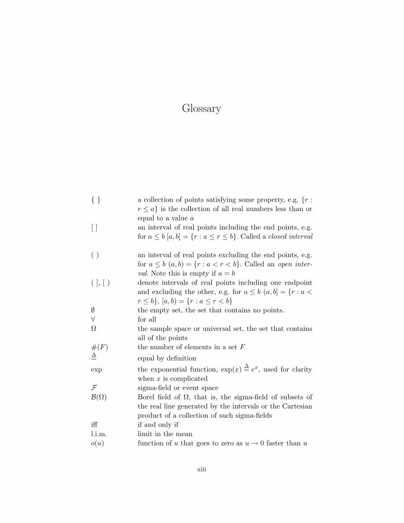
Glossary

a collection of points satisfying some property, e.g. r :

r ≤ a is the collection of all real numbers less than or

equal to a value a

[ ] an interval of real points including the end points, e.g.

for a ≤ b [a, b] = r : a ≤ r ≤ b. Called a closed interval

( ) an interval of real points excluding the end points, e.g.

for a ≤ b (a, b) = r : a < r < b. Called an open inter-

val. Note this is empty if a = b

( ], [ ) denote intervals of real points including one endpoint

and excluding the other, e.g. for a ≤ b (a, b] = r : a <

r ≤ b, [a, b) = r : a ≤ r < b∅ the empty set, the set that contains no points.

∀ for all

Ω the sample space or universal set, the set that contains

all of the points

#(F ) the number of elements in a set F∆= equal by definition

exp the exponential function, exp(x)∆= ex, used for clarity

when x is complicated

F sigma-field or event space

B(Ω) Borel field of Ω, that is, the sigma-field of subsets of

the real line generated by the intervals or the Cartesian

product of a collection of such sigma-fields

iff if and only if

l.i.m. limit in the mean

o(u) function of u that goes to zero as u → 0 faster than u

xiii

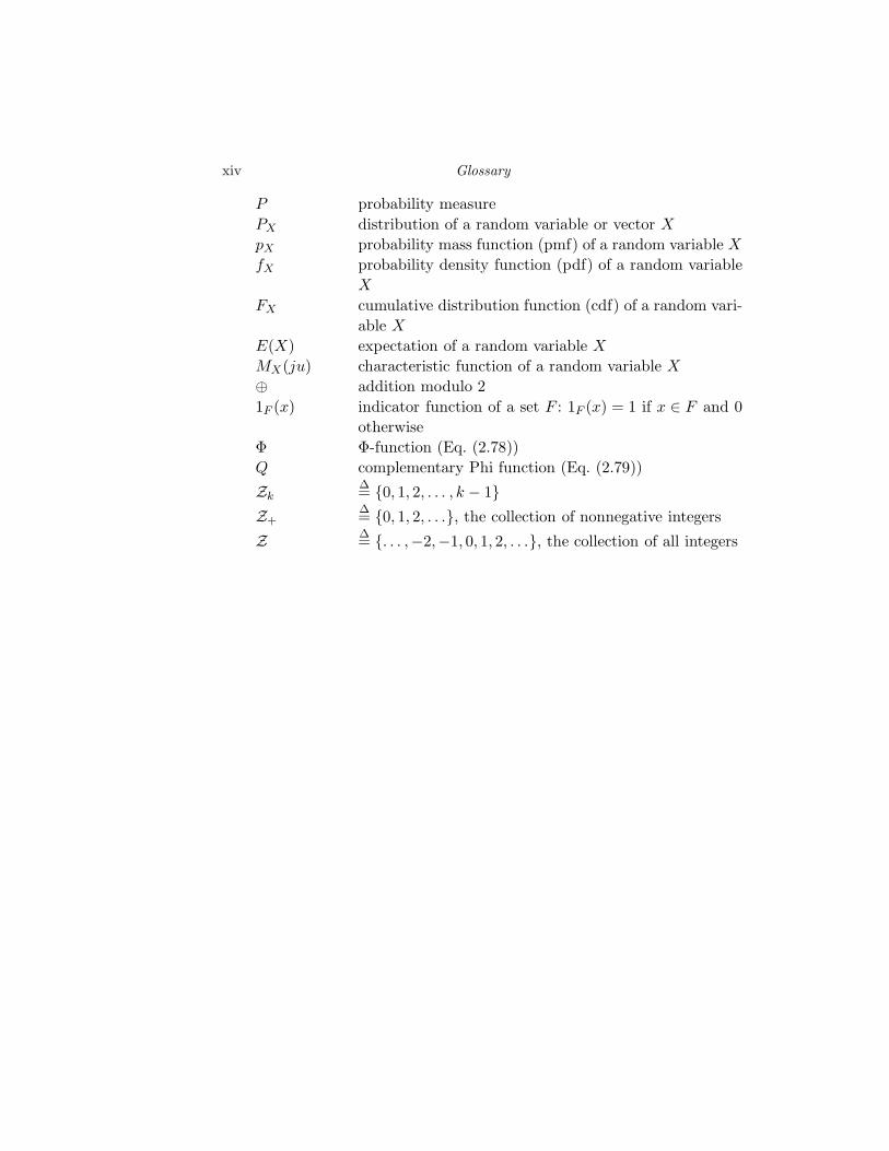
xiv Glossary

P probability measure

PX distribution of a random variable or vector X

pX probability mass function (pmf) of a random variable X

fX probability density function (pdf) of a random variable

X

FX cumulative distribution function (cdf) of a random vari-

able X

E(X) expectation of a random variable X

MX(ju) characteristic function of a random variable X

⊕ addition modulo 2

1F (x) indicator function of a set F : 1F (x) = 1 if x ∈ F and 0

otherwise

Φ Φ-function (Eq. (2.78))

Q complementary Phi function (Eq. (2.79))

Zk∆= 0, 1, 2, . . . , k − 1

Z+∆= 0, 1, 2, . . ., the collection of nonnegative integers

Z ∆= . . . ,−2,−1, 0, 1, 2, . . ., the collection of all integers

1

Introduction

A random or stochastic process is a mathematical model for a phenomenon

that evolves in time in an unpredictable manner from the viewpoint of the

observer. The phenomenon may be a sequence of real-valued measurements

of voltage or temperature, a binary data stream from a computer, a mod-

ulated binary data stream from a modem, a sequence of coin tosses, the

daily Dow–Jones average, radiometer data or photographs from deep space

probes, a sequence of images from a cable television, or any of an infinite

number of possible sequences, waveforms, or signals of any imaginable type.

It may be unpredictable because of such effects as interference or noise in a

communication link or storage medium, or it may be an information-bearing

signal, deterministic from the viewpoint of an observer at the transmitter

but random to an observer at the receiver.

The theory of random processes quantifies the above notions so that

one can construct mathematical models of real phenomena that are both

tractable and meaningful in the sense of yielding useful predictions of fu-

ture behavior. Tractability is required in order for the engineer (or anyone

else) to be able to perform analyses and syntheses of random processes, per-

haps with the aid of computers. The “meaningful” requirement is that the

models must provide a reasonably good approximation of the actual phe-

nomena. An oversimplified model may provide results and conclusions that

do not apply to the real phenomenon being modeled. An overcomplicated

one may constrain potential applications, render theory too difficult to be

useful, and strain available computational resources. Perhaps the most dis-

tinguishing characteristic between an average engineer and an outstanding

engineer is the ability to derive effective models providing a good balance

between complexity and accuracy.

Random processes usually occur in applications in the context of environ-

ments or systems which change the processes to produce other processes.

1

2 Introduction

The intentional operation on a signal produced by one process, an “input

signal,” to produce a new signal, an “output signal,” is generally referred to

as signal processing, a topic easily illustrated by examples.

• A time-varying voltage waveform is produced by a human speaking into a mi-

crophone or telephone. The signal can be modeled by a random process. This

signal might be modulated for transmission, then it might be digitized and coded

for transmission on a digital link. Noise in the digital link can cause errors in

reconstructed bits, the bits can then be used to reconstruct the original signal

within some fidelity. All of these operations on signals can be considered as signal

processing, although the name is most commonly used for manmade operations

such as modulation, digitization, and coding, rather than the natural possibly

unavoidable changes such as the addition of thermal noise or other changes out

of our control.

• For digital speech communications at very low bit rates, speech is sometimes

converted into a model consisting of a simple linear filter (called an autoregressive

filter) and an input process. The idea is that the parameters describing the model

can be communicated with fewer bits than can the original signal, but the receiver

can synthesize the human voice at the other end using the model so that it sounds

very much like the original signal. A system of this type is called a vocoder .

• Signals including image data transmitted from remote spacecraft are virtually

buried in noise added to them on route and in the front end amplifiers of the

receivers used to retrieve the signals. By suitably preparing the signals prior to

transmission, by suitable filtering of the received signal plus noise, and by suitable

decision or estimation rules, high quality images are transmitted through this very

poor channel.

• Signals produced by biomedical measuring devices can display specific behavior

when a patient suddenly changes for the worse. Signal processing systems can look

for these changes and warn medical personnel when suspicious behavior occurs.

• Images produced by laser cameras inside elderly North Atlantic pipelines can

be automatically analyzed to locate possible anomalies indicating corrosion by

looking for locally distinct random behavior.

How are these signals characterized? If the signals are random, how does one

find stable behavior or structures to describe the processes? How do opera-

tions on these signals change them? How can one use observations based on

random signals to make intelligent decisions regarding future behavior? All

of these questions lead to aspects of the theory and application of random

processes.

Courses and texts on random processes usually fall into either of two

general and distinct categories. One category is the common engineering

approach, which involves fairly elementary probability theory, standard un-

Introduction 3

dergraduate Riemann calculus, and a large dose of “cookbook” formulas –

often with insufficient attention paid to conditions under which the formu-

las are valid. The results are often justified by nonrigorous and occasionally

mathematically inaccurate handwaving or intuitive plausibility arguments

that may not reflect the actual underlying mathematical structure and may

not be supportable by a precise proof. While intuitive arguments can be

extremely valuable in providing insight into deep theoretical results, they

can be a handicap if they do not capture the essence of a rigorous proof.

A development of random processes that is insufficiently mathematical

leaves the student ill prepared to generalize the techniques and results when

faced with a real-world example not covered in the text. For example, if

one is faced with the problem of designing signal processing equipment for

predicting or communicating measurements being made for the first time

by a space probe, how does one construct a mathematical model for the

physical process that will be useful for analysis? If one encounters a process

that is neither stationary nor ergodic (terms we shall consider in detail),

what techniques still apply? Can the law of large numbers still be used to

construct a useful model?

An additional problem with an insufficiently mathematical development is

that it does not leave the student adequately prepared to read modern liter-

ature such as the many Transactions of the IEEE and the journals of the Eu-

ropean Association for Signal, Speech, and Image Processing (EURASIP).

The more advanced mathematical language of recent work is increasingly

used even in simple cases because it is precise and universal and focuses on

the structure common to all random processes. Even if an engineer is not

directly involved in research, knowledge of the current literature can often

provide useful ideas and techniques for tackling specific problems. Engineers

unfamiliar with basic concepts such as sigma-field and conditional expecta-

tion will find many potentially valuable references shrouded in mystery.

The other category of courses and texts on random processes is the typical

mathematical approach, which requires an advanced mathematical back-

ground of real analysis, measure theory, and integration theory. This ap-

proach involves precise and careful theorem statements and proofs, and uses

far more care to specify precisely the conditions required for a result to

hold. Most engineers do not, however, have the required mathematical back-

ground, and the extra care required in a completely rigorous development

severely limits the number of topics that can be covered in a typical course

– in particular, the applications that are so important to engineers tend to

be neglected. In addition, too much time is spent with the formal details,

4 Introduction

obscuring the often simple and elegant ideas behind a proof. Often little, if

any, physical motivation for the topics is given.

This book attempts a compromise between the two approaches by giving

the basic theory and a profusion of examples in the language and notation

of the more advanced mathematical approaches. The intent is to make the

crucial concepts clear in the traditional elementary cases, such as coin flip-

ping, and thereby to emphasize the mathematical structure of all random

processes in the simplest possible context. The structure is then further de-

veloped by numerous increasingly complex examples of random processes

that have proved useful in systems analysis. The complicated examples are

constructed from the simple examples by signal processing, that is, by using

a simple process as an input to a system whose output is the more com-

plicated process. This has the double advantage of describing the action of

the system, the actual signal processing, and the interesting random process

which is thereby produced. As one might suspect, signal processing also can

be used to produce simple processes from complicated ones.

Careful proofs are usually constructed only in elementary cases. For ex-

ample, the fundamental theorem of expectation is proved only for discrete

random variables, where it is proved simply by a change of variables in a

sum. The continuous analog is subsequently given without a careful proof,

but with the explanation that it is simply the integral analog of the sum-

mation formula and hence can be viewed as a limiting form of the discrete

result. As another example, only weak laws of large numbers are proved in

detail in the mainstream of the text, but the strong law is treated in detail

for a special case in a starred section. Starred sections are used to delve

into other relatively advanced results, for example the use of mean square

convergence ideas to make rigorous the notion of integration and filtering of

continuous time processes.

By these means we strive to capture the spirit of important proofs with-

out undue tedium and to make plausible the required assumptions and con-

straints. This, in turn, should aid the student in determining when certain

tools do or do not apply and what additional tools might be necessary when

new generalizations are required.

A distinct aspect of the mathematical viewpoint is the “grand experiment”

view of random processes as being a probability measure on sequences (for

discrete time) or waveforms (for continuous time) rather than being an infin-

ity of smaller experiments representing individual outcomes (called random

variables) that are somehow glued together. From this point of view random

variables are merely special cases of random processes. In fact, the grand ex-

Introduction 5

periment viewpoint was popular in the early days of applications of random

processes to systems and was called the “ensemble” viewpoint in the work of

Norbert Wiener and his students. By viewing the random process as a whole

instead of as a collection of pieces, many basic ideas, such as stationarity

and ergodicity, that characterize the dependence on time of probabilistic de-

scriptions and the relation between time averages and probabilistic averages

are much easier to define and study. This also permits a more complete dis-

cussion of processes that violate such probabilistic regularity requirements

yet still have useful relations between time and probabilistic averages.

Even though a student completing this book will not be able to follow

the details in the literature of many proofs of results involving random pro-

cesses, the basic results and their development and implications should be

accessible, and the most common examples of random processes and classes

of random processes should be familiar. In particular, the student should

be well equipped to follow the gist of most arguments in the various Trans-

actions of the IEEE dealing with random processes, including the IEEE

Transactions on Signal Processing, IEEE Transactions on Image Processing,

IEEE Transactions on Speech and Audio Processing, IEEE Transactions on

Communications, IEEE Transactions on Control, and IEEE Transactions

on Information Theory, and the EURASIP/Elsevier journals such as Image

Communication, Speech Communication, and Signal Processing.

It also should be mentioned that the authors are electrical engineers and,

as such, have written this text with an electrical engineering flavor. How-

ever, the required knowledge of classical electrical engineering is slight, and

engineers in other fields should be able to follow the material presented.

This book is intended to provide a one-quarter or one-semester course

that develops the basic ideas and language of the theory of random pro-

cesses and provides a rich collection of examples of commonly encountered

processes, properties, and calculations. Although in some cases these exam-

ples may seem somewhat artificial, they are chosen to illustrate the way

engineers should think about random processes. They are selected for sim-

plicity and conceptual content rather than to present the method of solution

to some particular application. Sections that can be skimmed or omitted for

the shorter one-quarter curriculum are marked with a star (⋆). Discrete time

processes are given more emphasis than in many texts because they are sim-

pler to handle and because they are of increasing practical importance in

digital systems. For example, linear filter input/output relations are carefully

developed for discrete time; then the continuous time analogs are obtained

6 Introduction

by replacing sums with integrals. The mathematical details underlying the

continuous time results are found in a starred section.

Most examples are developed by beginning with simple processes. These

processes are filtered or modulated to obtain more complicated processes.

This provides many examples of typical probabilistic computations on simple

processes and on the output of operations on simple processes. Extra tools

are introduced as needed to develop properties of the examples.

The prerequisites for this book are elementary set theory, elementary prob-

ability, and some familiarity with linear systems theory (Fourier analysis,

convolution, discrete and continuous time linear filters, and transfer func-

tions). The elementary set theory and probability may be found, for example,

in the classic text by Al Drake [18] or in the current MIT basic probability

text by Bertsekas and Tsitsiklis [3]. The Fourier and linear systems material

can by found in numerous texts, including Gray and Goodman [33]. Some of

these basic topics are reviewed in this book in Appendix A. These results are

considered prerequisite as the pace and density of material would likely be

overwhelming to someone not already familiar with the fundamental ideas

of probability such as probability mass and density functions (including the

more common named distributions), computing probabilities, derived dis-

tributions, random variables, and expectation. It has long been the authors’

experience that the students having the most difficulty with this material

are those with little or no experience with elementary probability.

Organization of the book

Chapter 2 provides a careful development of the fundamental concept

of probability theory – a probability space or experiment. The notions of

sample space, event space, and probability measure are introduced and il-

lustrated by examples. Independence and elementary conditional probability

are developed in some detail. The ideas of signal processing and of random

variables are introduced briefly as functions or operations on the output of

an experiment. This in turn allows mention of the idea of expectation at an

early stage as a generalization of the description of probabilities by sums or

integrals.

Chapter 3 treats the theory of measurements made on experiments:

random variables, which are scalar-valued measurements; random vectors,

which are a vector or finite collection of measurements; and random pro-

cesses, which can be viewed as sequences or waveforms of measurements.

Introduction 7

Random variables, vectors, and processes can all be viewed as forms of sig-

nal processing: each operates on “inputs,” which are the sample points of

a probability space, and produces an “output,” which is the resulting sam-

ple value of the random variable, vector, or process. These output points

together constitute an output sample space, which inherits its own proba-

bility measure from the structure of the measurement and the underlying

experiment. As a result, many of the basic properties of random variables,

vectors, and processes follow from those of probability spaces. Probability

distributions are introduced along with probability mass functions, prob-

ability density functions, and cumulative distribution functions. The basic

derived distribution method is described and demonstrated by example. A

wide variety of examples of random variables, vectors, and processes are

treated. Expectations are introduced briefly as a means of characterizing

distributions and to provide some calculus practice.

Chapter 4 develops in depth the ideas of expectation – averages of random

objects with respect to probability distributions. Also called probabilistic

averages, statistical averages, and ensemble averages, expectations can be

thought of as providing simple but important parameters describing proba-

bility distributions. A variety of specific averages are considered, including

mean, variance, characteristic functions, correlation, and covariance. Several

examples of unconditional and conditional expectations and their properties

and applications are provided. Perhaps the most important application is

to the statement and proof of laws of large numbers or ergodic theorems,

which relate long-term sample-average behavior of random processes to ex-

pectations. In this chapter laws of large numbers are proved for simple, but

important, classes of random processes. Other important applications of ex-

pectation arise in performing and analyzing signal processing applications

such as detecting, classifying, and estimating data. Minimum mean squared

nonlinear and linear estimation of scalars and vectors is treated in some de-

tail, showing the fundamental connections among conditional expectation,

optimal estimation, and second-order moments of random variables and vec-

tors.

Chapter 5 concentrates on the computation and applications of second-

order moments – the mean and covariance – of a variety of random pro-

cesses. The primary example is a form of derived distribution problem: if

a given random process with known second-order moments is put into a

linear system what are the second-order moments of the resulting output

random process? This problem is treated for linear systems represented by

convolutions and for linear modulation systems. Transform techniques are

8 Introduction

shown to provide a simplification in the computations, much like their ordi-

nary role in elementary linear systems theory. Mean square convergence is

revisited and several of its applications to the analysis of continuous time

random processes are collected under the heading of mean square calcu-

lus. Included are a careful definition of integration and filtering of random

processes, differentiation of random processes, and sampling and orthogonal

expansions of random processes. In all of these examples the behavior of

the second-order moments determines the applicability of the results. The

chapter closes with a development of several results from the theory of linear

least squares estimation. This provides an example of both the computation

and the application of second-order moments.

In Chapter 6 a variety of useful models of sometimes complicated ran-

dom processes are developed. A powerful approach to modeling complicated

random processes is to consider linear systems driven by simple random

processes. Chapter 5 used this approach to compute second-order moments,

this chapter goes beyond moments to develop a complete description of the

output processes. To accomplish this, however, one must make additional

assumptions on the input process and on the form of the linear filters. The

general model of a linear filter driven by a memoryless process is used to

develop several popular models of discrete time random processes. Analo-

gous continuous time random process models are then developed by direct

description of their behavior. The principal class of random processes con-

sidered is the class of independent increment processes, but other processes

with similar definitions but quite different properties are also introduced.

Among the models considered are autoregressive processes, moving-average

processes, ARMA (autoregressive moving-average) processes, random walks,

independent increment processes, Markov processes, Poisson and Gaussian

processes, and the random telegraph wave process. We also briefly consider

an example of a nonlinear system where the output random processes can

at least be partially described – the exponential function of a Gaussian or

Poisson process which models phase or frequency modulation. We close with

examples of a type of “doubly stochastic” process – a compound process

formed by adding a random number of other random effects.

Appendix A sketches several prerequisite definitions and concepts from

elementary set theory and linear systems theory using examples to be en-

countered elsewhere in the book. The first subject is crucial at an early stage

and should be reviewed before proceeding to Chapter 2. The second sub-

ject is not required until Chapter 5, but it serves as a reminder of material

with which the student should already be familiar. Elementary probability

Introduction 9

is not reviewed, as our basic development includes elementary probability

presented in a rigorous manner that sets the stage for more advanced prob-

ability. The review of prerequisite material in the appendix serves to collect

together some notation and many definitions that will be used throughout

the book. It is, however, only a brief review and cannot serve as a substitute

for a complete course on the material. This chapter can be given as a first

reading assignment and either skipped or skimmed briefly in class; lectures

can proceed from an introduction, perhaps incorporating some preliminary

material, directly to Chapter 2.

Appendix B provides some scattered definitions and results needed in

the book that detract from the main development, but may be of interest

for background or detail. These fall primarily in the realm of calculus and

range from the evaluation of common sums and integrals to a consideration

of different definitions of integration. Many of the sums and integrals should

be prerequisite material, but it has been the authors’ experience that many

students have either forgotten or not seen many of the standard tricks.

Hence several of the most important techniques for probability and signal

processing applications are included. Also in this appendix some background

information on limits of double sums and the Lebesgue integral is provided.

Appendix C collects the common univariate probability mass functions

and probability density functions along with their second-order moments

for reference.

The book concludes with Appendix D suggesting supplementary reading,

providing occasional historical notes, and delving deeper into some of the

technical issues raised in the book. In that section we assemble references on

additional background material as well as on books that pursue the various

topics in more depth or on a more advanced level. We feel that these com-

ments and references are supplementary to the development and that less

clutter results by putting them in a single appendix rather than strewing

them throughout the text. The section is intended as a guide for further

study, not as an exhaustive description of the relevant literature, the latter

goal being beyond the authors’ interests and stamina.

Each chapter is accompanied by a collection of problems, many of which

have been contributed by collegues, readers, students, and former students.

It is important when doing the problems to justify any “yes/no” answers.

If an answer is “yes,” prove it is so. If the answer is “no,” provide a coun-

terexample.

2

Probability

2.1 Introduction

The theory of random processes is a branch of probability theory and proba-

bility theory is a special case of the branch of mathematics known as measure

theory. Probability theory and measure theory both concentrate on functions

that assign real numbers to certain sets in an abstract space according to

certain rules. These set functions can be viewed as measures of the size or

weight of the sets. For example, the precise notion of area in two-dimensional

Euclidean space and volume in three-dimensional space are both examples

of measures on sets. Other measures on sets in three dimensions are mass

and weight. Observe that from elementary calculus we can find volume by

integrating a constant over the set. From physics we can find mass by inte-

grating a mass density or summing point masses over a set. In both cases the

set is a region of three-dimensional space. In a similar manner, probabilities

will be computed by integrals of densities of probability or sums of “point

masses” of probability.

Both probability theory and measure theory consider only nonnegative

real-valued set functions. The value assigned by the function to a set is called

the probability or the measure of the set, respectively. The basic difference

between probability theory and measure theory is that the former considers

only set functions that are normalized in the sense of assigning the value

of 1 to the entire abstract space, corresponding to the intuition that the

abstract space contains every possible outcome of an experiment and hence

should happen with certainty or probability 1. Subsets of the space have

some uncertainty and hence have probability less than 1.

Probability theory begins with the concept of a probability space, which

is a collection of three items:

1. An abstract space Ω, as encountered in Appendix A, called a sample space, which

10

2.1 Introduction 11

contains all distinguishable elementary outcomes or results of an experiment.

These points might be names, numbers, or complicated signals.

2. An event space or sigma-field F consisting of a collection of subsets of the ab-

stract space which we wish to consider as possible events and to which we wish to

assign a probability. We require that the event space have an algebraic structure

in the following sense: any finite or countably infinite sequence of set-theoretic

operations (union, intersection, complementation, difference, symmetric differ-

ence) on events must produce other events.

3. A probability measure P – an assignment of a number between 0 and 1 to ev-

ery event, that is, to every set in the event space. A probability measure must

obey certain rules or axioms and will be computed by integrating or summing,

analogously to area, volume, and mass computations.

This chapter is devoted to developing the ideas underlying the triple

(Ω,F , P ), which is collectively called a probability space or an experiment.

Before making these ideas precise, however, several comments are in order.

First of all, it should be emphasized that a probability space is composed

of three parts; an abstract space is only one part. Do not let the termi-

nology confuse you: “space” has more than one usage. Having an abstract

space model all possible distinguishable outcomes of an experiment should

be an intuitive idea since it simply gives a precise mathematical name to

an imprecise English description. Since subsets of the abstract space corre-

spond to collections of elementary outcomes, it should also be possible to

assign probabilities to such sets. It is a little harder to see, but we can also

argue that we should focus on the sets and not on the individual points

when assigning probabilities since in many cases a probability assignment

known only for points will not be very useful. For example, if we spin a

pointer and the outcome is known to be equally likely to be any number

between 0 and 1, then the probability that any particular point such as

0.3781984637 or exactly 1/π occurs is zero because there is an uncountable

infinity of possible points, none more likely than the others1.Hence knowing

only that the probability of each and every point is zero, we would be hard

pressed to make any meaningful inferences about the probabilities of other

events such as the outcome being between 1/2 and 3/4. Writers of fiction

(including Patrick O’Brian in his Aubrey–Maturin series) have made much

of the fact that extremely unlikely events often occur. One can say that zero

1 A set is countably infinite if it can be put into one-to-one correspondence with thenonnegative integers and hence can be counted. For example, the set of positiveintegers is countable and the set of all rational numbers is countable. The set ofall irrational numbers and the set of all real numbers are both uncountable. SeeAppendix A for a discussion of countably infinite vs. uncountably infinite spaces.

12 Probability

probability events occur virtually all the time since the a-prioriprobability

that the Universe will be exactly in a particular configuration at 13:15 Co-

ordinated Universal Time (also known as Greenwich Mean Time) is zero,

yet the Universe will indeed be in some configuration at that time.

The difficulty inherent in this example leads to a less natural aspect of

the probability space triumvirate – the fact that we must specify an event

space or collection of subsets of our abstract space to which we wish to as-

sign probabilities. In the example it is clear that taking the individual points

and their countable combinations is not enough (see also Problem 2.3). On

the other hand, why not just make the event space the class of all subsets of

the abstract space? Why require the specification of which subsets are to be

deemed sufficiently important to be blessed with the name “event”? In fact,

this concern is one of the principal differences between elementary proba-

bility theory and advanced probability theory (and the point at which the

student’s intuition frequently runs into trouble). When the abstract space is

finite or even countably infinite, one can consider all possible subsets of the

space to be events, and one can build a useful theory. When the abstract

space is uncountably infinite, however, as in the case of the space consisting

of the real line or the unit interval, one cannot build a useful theory with-

out constraining the subsets to which one will assign a probability. Roughly

speaking, this is because probabilities of sets in uncountable spaces are found

by integrating over sets, and some sets are simply too nasty to be integrated

over. Although it is difficult to show, for such spaces there does not exist

a reasonable and consistent means of assigning probabilities to all subsets

without contradiction or without violating desirable properties. In fact, it is

so difficult to show that such “non-probability-measurable” subsets of the

real line exist that we will not attempt to do so in this book. The reader

should at least be aware of the problem so that the need for specifying an

event space is understood. It also explains why the reader is likely to en-

counter phrases like “measurable sets” and “measurable functions” in the

literature – some things are unmeasurable!

Thus a probability space must make explicit not just the elementary out-

comes or “finest-grain” outcomes that constitute our abstract space; it must

also specify the collections of sets of these points to which we intend to assign

probabilities. Subsets of the abstract space that do not belong to the event

space will simply not have probabilities defined. The algebraic structure that

we have postulated for the event space will ensure that if we take (countable)

unions of events (corresponding to a logical “or”) or intersections of events

(corresponding to a logical “and”), then the resulting sets are also events

2.1 Introduction 13

and hence will have probabilities. In fact, this is one of the main functions of

probability theory: given a probabilistic description of a collection of events,

find the probability of some new event formed by set-theoretic operations

on the given events.

Up to this point the notion of signal processing has not been mentioned.

It enters at a fundamental level if one realizes that each individual point

ω ∈ Ω produced in an experiment can be viewed as a signal : it might be

a single voltage conveying the value of a measurement, a vector of values,

a sequence of values, or a waveform, any one of which can be interpreted

as a signal measured in the environment or received from a remote trans-

mitter or extracted from a physical medium that was previously recorded.

Signal processing in general is the performing of some operation on the sig-

nal. In its simplest yet most general form this consists of applying some

function or mapping or operation g to the signal or input ω to produce

an output g(ω), which might be intended to guess some hidden parameter,

extract useful information from noise, or enhance an image, or might be

any simple or complicated operation intended to produce a useful outcome.

If we have a probabilistic description of the underlying experiment, then

we should be able to derive a probabilistic description of the outcome of

the signal processor. This is the core problem of derived distributions, one

of the fundamental tools of both probability theory and signal processing.

In fact, this idea of defining functions on probability spaces is the foun-

dation for the definition of random variables, random vectors, and random

processes, which will inherit their basic properties from the underlying prob-

ability space, thereby yielding new probability spaces. Much of the theory

of random processes and signal processing consists of developing the im-

plications of certain operations on probability spaces: beginning with some

probability space we form new ones by operations called variously mappings,

filtering, sampling, coding, communicating, estimating, detecting, averaging,

measuring, enhancing, predicting, smoothing, interpolating, classifying, an-

alyzing, or other names denoting linear or nonlinear operations. Stochastic

systems theory is the combination of systems theory with probability theory.

The essence of stochastic systems theory is the connection of a system to

a probability space. Thus a precise formulation and a good understanding

of probability spaces are prerequisites to a precise formulation and correct

development of examples of random processes and stochastic systems.

Before proceeding to a careful development, several of the basic ideas are

illustrated informally with simple examples.

14 Probability

2.2 Spinning pointers and flipping coins

Many of the basic ideas at the core of this text can be introduced and illus-

trated by two very simple examples, the continuous experiment of spinning

a pointer inside a circle and the discrete experiment of flipping a coin.

A uniform spinning pointer

Suppose that Nature (or perhaps Tyche, the Greek goddess of chance)

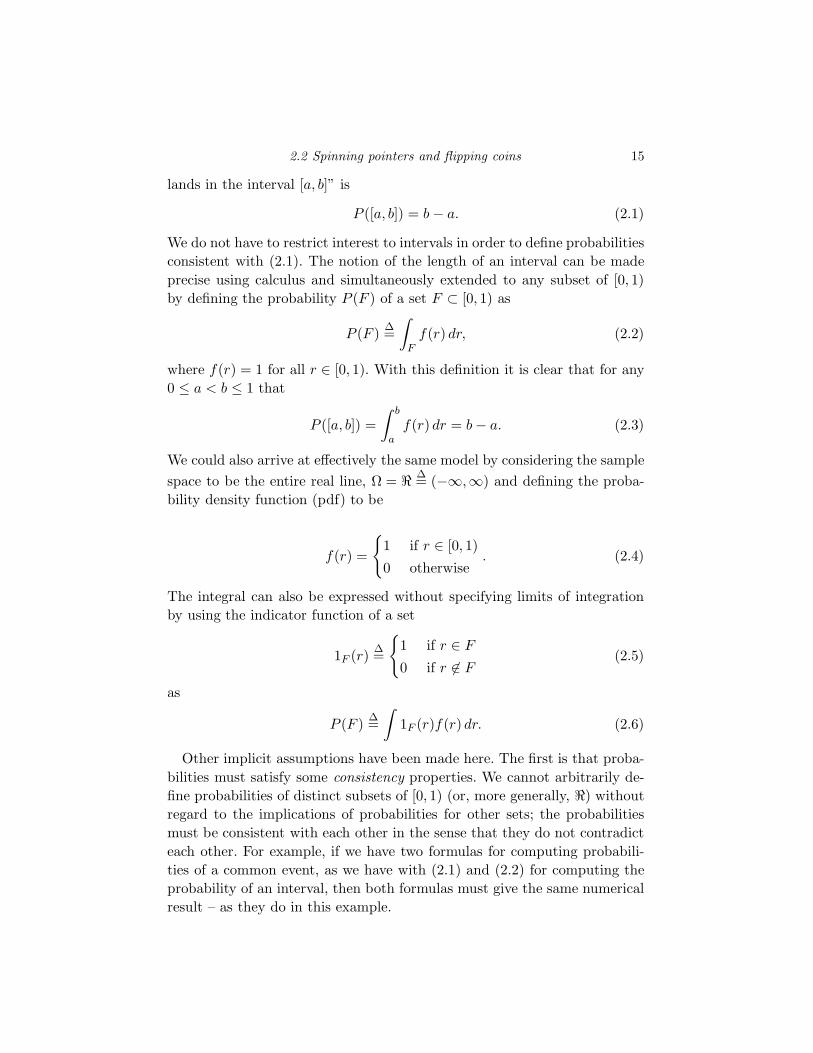
spins a pointer in a circle as depicted in Figure 2.1. When the pointer stops

&%'$

60.0

0.5

0.250.75

Figure 2.1 The spinning pointer

it can point to any number in the unit interval [0, 1)∆= r : 0 ≤ r < 1. We

call [0, 1) the sample space of our experiment and denote it by a capital

Greek omega, Ω. What can we say about the probabilities or chances of

particular events or outcomes occurring as a result of this experiment? The

sorts of events of interest are things like “the pointer points to a number

between 0.0 and 0.5” (which one would expect should have probability 0.5

if the wheel is indeed fair) or “the pointer does not lie between 0.75 and

1” (which should have a probability of 0.75). Two assumptions are implicit

here. The first is that an “outcome” of the experiment or an “event” to

which we can assign a probability is simply a subset of [0, 1). The second

assumption is that the probability of the pointer landing in any particular

interval of the sample space is proportional to the length of the interval.

This should seem reasonable if we indeed believe the spinning pointer to be

“fair” in the sense of not favoring any outcomes over any others. The bigger

a region of the circle, the more likely the pointer is to end up in that region.

We can formalize this by stating that for any interval [a, b] = r : a ≤ r ≤ bwith 0 ≤ a ≤ b < 1 we have that the probability of the event “the pointer

2.2 Spinning pointers and flipping coins 15

lands in the interval [a, b]” is

P ([a, b]) = b − a. (2.1)

We do not have to restrict interest to intervals in order to define probabilities

consistent with (2.1). The notion of the length of an interval can be made

precise using calculus and simultaneously extended to any subset of [0, 1)

by defining the probability P (F ) of a set F ⊂ [0, 1) as

P (F )∆=

∫

Ff(r) dr, (2.2)

where f(r) = 1 for all r ∈ [0, 1). With this definition it is clear that for any

0 ≤ a < b ≤ 1 that

P ([a, b]) =

∫ b

af(r) dr = b − a. (2.3)

We could also arrive at effectively the same model by considering the sample

space to be the entire real line, Ω = ℜ ∆= (−∞,∞) and defining the proba-

bility density function (pdf) to be

f(r) =

1 if r ∈ [0, 1)

0 otherwise. (2.4)

The integral can also be expressed without specifying limits of integration

by using the indicator function of a set

1F (r)∆=

1 if r ∈ F

0 if r 6∈ F(2.5)

as

P (F )∆=

∫1F (r)f(r) dr. (2.6)

Other implicit assumptions have been made here. The first is that proba-

bilities must satisfy some consistency properties. We cannot arbitrarily de-

fine probabilities of distinct subsets of [0, 1) (or, more generally, ℜ) without

regard to the implications of probabilities for other sets; the probabilities

must be consistent with each other in the sense that they do not contradict

each other. For example, if we have two formulas for computing probabili-

ties of a common event, as we have with (2.1) and (2.2) for computing the

probability of an interval, then both formulas must give the same numerical

result – as they do in this example.

16 Probability

The second implicit assumption is that the integral exists in a well-defined

sense, that it can be evaluated using calculus. As surprising as it may seem

to readers familiar only with typical engineering-oriented developments of

Riemann integration, the integral of (2.2) is in fact not well defined for

all subsets of [0, 1). But we leave this detail for later and assume for the

moment that we only encounter sets for which the integral (and hence the

probability) is well defined.

The function f(r) is called a probability density function or pdf since it is a

nonnegative point function that is integrated to compute total probability of

a set, just as a mass density function is integrated over a region to compute

the mass of a region in physics. Since in this example f(r) is constant over

a region, it is called a uniform pdf.

The formula (2.2) for computing probability has many implications, three

of which merit comment at this point.

• Probabilities are nonnegative:

P (F ) ≥ 0 for any F. (2.7)

This follows since integrating a nonnegative argument yields a nonnegative result.

• The probability of the entire sample space is 1:

P (Ω) = 1. (2.8)

This follows since integrating 1 over the unit interval yields 1, but it has the

intuitive interpretation that the probability that “something happens” is 1.

• The probability of the union of disjoint or mutually exclusive regions is the sum

of the probabilities of the individual events:

If F ∩ G = ∅, then P (F ∪ G) = P (F ) + P (G). (2.9)

This follows immediately from the properties of integration:

P (F ∪ G) =

∫

F∪G

f(r) dr =

∫

F

f(r) dr +

∫

G

f(r) dr

= P (F ) + P (G).

An alternative proof of the third property follows by observing that since F

and G are disjoint, 1F∪G(r) = 1F (r) + 1G(r) and hence linearity of integra-

tion implies that

P (F ∪ G) =

∫1F∪G(r)f(r) dr =

∫(1F (r) + 1G(r))f(r) dr

=

∫1F (r)f(r) dr +

∫1G(r)f(r) dr

= P (F ) + P (G).

2.2 Spinning pointers and flipping coins 17

This property is often called the additivity property of probability. The sec-

ond proof makes it clear that additivity of probability is an immediate result

of the linearity of integration, i.e., that the integral of the sum of two func-

tions is the sum of the two integrals.

Repeated application of additivity for two events shows that for any fi-

nite collection Fk; k = 1, 2, . . . ,K of disjoint events, i.e., events with the

property that Fk

⋂Fj = ∅ for all k 6= j, we have that

P

(K⋃

k=1

Fk

)=

K∑

k=1

P (Fk), (2.10)

showing that additivity is equivalent to finite additivity , the extension of the

additivity property from two to a finite collection of sets. Since additivity

is a special case of finite additivity and it implies finite additivity, the two

notions are equivalent and we can use them interchangeably.

These three properties of nonnegativity, normalization, and additivity are

fundamental to the definition of the general notion of probability and will

form three of the four axioms needed for a precise development. It is tempt-

ing to call an assignment P of numbers to subsets of a sample space a

probability measure if it satisfies these three properties, but we shall see

that a fourth condition, which is crucial for having well-behaved limits and

asymptotics, will be needed to complete the definition. Pending this fourth

condition, (2.2) defines a probability measure. In fact, this definition is com-

plete in the simple case where the sample space Ω has only a finite number

of points since in that case limits and asympotics become trivial. A sample

space together with a probability measure provide a mathematical model

for an experiment. This model is often called a probability space, but for the

moment we shall stick to the less intimidating word of experiment.

Simple properties

Several simple properties of probabilities can be derived from what we

have so far. As particularly simple, but still important, examples, consider

the following.

Assume that P is a set function defined on a sample space Ω that satisfies

the properties of equations (2.7)–(2.9). Then

(a) P (F c) = 1 − P (F ).

(b) P (F ) ≤ 1.

(c) Let ∅ be the null or empty set, then P (∅) = 0.

18 Probability

(d) If Fi; i = 1, 2, . . . ,K is a finite partition of Ω, i.e., if Fi ∩ Fk = ∅when i 6= k and

⋃i=1 Fi = Ω, then

P (G) =

K∑

i=1

P (G ∩ Fi) (2.11)

for any event G.

Proof

(a) F ∪ F c = Ω implies P (F ∪ F c) = 1 (Property (2.8)). F ∩ F c = ∅ im-

plies 1 = P (F ∪ F c) = P (F ) + P (F c) (Property (2.9)).

(b) P (F ) = 1 − P (F c) ≤ 1 (Property (2.7) and (a) above).

(c) By Property (2.8) and (a) above, P (Ωc) = P (∅) = 1 − P (Ω) = 0.

(d) P (G) = P (G ∩ Ω) = P (G ∩ (⋃

iFi)) = P (⋃

i(G ∩ Fi)) =∑

iP (G ∩Fi). 2

Observe that although the null or empty set ∅ has probability 0, the converse

is not true in that a set need not be empty just because it has zero probabil-

ity. In the uniform fair wheel example the set F = 1/n : n = 1, 2, 3, . . . is

not empty, but it does have probability zero. This follows roughly because

for any finite N P (1/n : n = 2, 3, . . . , N) = 0 (since the integral of 1 over

a finite set of points is zero) and therefore the limit as N → ∞ must also be

zero, a “continuity of probability” idea that we shall later make rigorous.

A single coin flip

The original example of a spinning wheel is continuous in that the sample

space consists of a continuum of possible outcomes, all points in the unit

interval. Sample spaces can also be discrete, as is the case of modeling a

single flip of a “fair” coin with heads labeled “1” and tails labeled “0”,

i.e., heads and tails are equally likely. The sample space in this example is

Ω = 0, 1 and the probability for any event or subset of Ω can be defined

in a reasonable way by

P (F ) =∑

r∈F

p(r), (2.12)

or, equivalently,

P (F ) =∑

1F (r)p(r), (2.13)

2.2 Spinning pointers and flipping coins 19

where now p(r) = 1/2 for each r ∈ Ω. The function p is called a probabil-

ity mass function or pmf because it is summed over points to find total

probability, just as point masses are summed to find total mass in physics.

Be cautioned that P is defined for sets and p is defined only for points in

the sample space. This can be confusing when dealing with one-point or

singleton sets, for example

P (0) = p(0)

P (1) = p(1).

This may seem too much work for such a little example, but keep in mind

that the goal is a formulation that will work for far more complicated and

interesting examples. This example is different from the spinning wheel in

that the sample space is discrete instead of continuous and that the prob-

abilities of events are defined by sums instead of integrals, as one should

expect when doing discrete mathematics. It is easy to verify, however, that

the basic properties (2.7)–(2.9) hold in this case as well (since sums behave

like integrals), which in turn implies that the simple properties (a)–(d) also

hold.

A single coin flip as signal processing

The coin flip example can also be derived in a very different way that

provides our first example of signal processing. Consider again the spinning

pointer so that the sample space is Ω and the probability measure P is

described by (2.2) using a uniform pdf as in (2.4). Performing the experi-

ment by spinning the pointer will yield some real number r ∈ [0, 1). Define

a measurement q made on this outcome by

q(r) =

1 if r ∈ [0, 0.5]

0 if r ∈ (0.5, 1). (2.14)

This function can also be defined somewhat more economically in terms of

an indicator function as

q(r) = 1[0,0.5](r). (2.15)

This is an example of a quantizer , an operation that maps a continuous

value into a discrete value. Quantization is an example of signal processing

since it is a function or mapping defined on an input space, here Ω = [0, 1) or

20 Probability

Ω = ℜ, producing a value in some output space. In this example Ωq = 0, 1.The dependence of a function on its input space or domain of definition Ω

and its output space or range Ωq,is often denoted by q : Ω → Ωq. Although

introduced as an example of simple signal processing, the usual name for a

real-valued function defined on the sample space of a probability space is

a random variable. We shall see in the next chapter that there is an extra

technical condition on functions to merit this name, but that is a detail that

can be postponed.

The output space Ωq can be considered as a new sample space, the space

corresponding to the possible values seen by an observer of the output of the

quantizer (an observer who might not have access to the original space). If

we know both the probability measure on the input space and the function,

then in theory we should be able to describe the probability measure that

the output space inherits from the input space. Since the output space is

discrete, it should be described by a pmf, say pq. Since there are only two

points, we need only find the value of pq(1) (or pq(0) since pq(0) + pq(1) = 1).

An output of 1 is seen if and only if the input sample point lies in [0, 0.5],

so it follows easily that pq(1) = P ([0, 0.5]) =∫ 0.50 f(r) dr = 0.5, exactly the

value assumed for the fair coin flip model. The pmf pq implies a probability

measure Pq on the output space Ωq defined by

Pq(F ) =∑

ω∈F

pq(ω),

where the subscript q distinguishes the probability measure Pq on the output

space from the probability measure P on the input space. Note that we can

define any other binary quantizer corresponding to an “unfair” or biased

coin by changing the 0.5 to some other value.

This simple example makes several fundamental points that will evolve in

depth in the course of this material. First, it provides an example of signal

processing and the first example of a random variable, which is essentially

just a mapping of one sample space into another. Second, it provides an

example of a derived distribution: given a probability space described by Ω

and P and a function (random variable) q defined on this space, we have

derived a new probability space describing the outputs of the function with

sample space Ωq and probability measure Pq. Third, it is an example of

a common phenomenon that quite different models can result in identical

sample spaces and probability measures. Here the coin flip could be modeled

in a directly given fashion by just describing the sample space and the prob-

ability measure, or it could be modeled in an indirect fashion as a function

(signal processing, random variable) on another experiment. This suggests,

2.2 Spinning pointers and flipping coins 21

for example, that to study coin flips empirically we could either actually flip

a fair coin, or we could spin a fair wheel and quantize the output. Although

the second method seems more complicated, it is in fact extremely common

since most random number generators (or pseudo-random number genera-

tors) strive to produce random numbers with a uniform distribution on [0, 1)

and all other probability measures are produced by further signal processing.

We have seen how to do this for a simple coin flip. In fact any pdf or pmf

can be generated in this way. (See Problem 3.7.) The generation of uniform

random numbers is both a science and an art. Most function roughly as fol-

lows. One begins with a floating point number in (0, 1) called the seed, say a,

and uses another positive floating point number, say b, as a multiplier. A se-

quence xn is then generated recursively as x0 = a and xn = b × xn−1 mod (1)

for n = 1, 2, . . ., that is, the fractional part of b × xn−1. If the two numbers

a and b are suitably chosen then xn should appear to be uniform. (Try it!)

In fact, since there are only a finite number (albeit large) of possible num-

bers that can be represented on a digital computer, this algorithm must

eventually repeat and hence xn must be a periodic sequence. As a result

such a sequence of numbers is a pseudo-random sequence and not a genuine

sequence of random numbers. The goal of designing a good pseudo-random

number generater is to make the period as long as possible and to make

the sequences produced look as much as possible like a random sequence in

the sense that statistical tests for independence are fooled. If one wanted to

generate a truly random generator, one might use some natural phenomenon

such as thermal noise, treated near the end of the book – measure the voltage

across a heated resistor and let the random action of molecules in motion

produce a random measurement.

Abstract versus concrete

It may seem strange that the axioms of probability deal with apparently

abstract ideas of measures instead of corresponding to physical intuition.

Physical intuition says that the probability tells you something about the

fraction of times specific events will occur in a sequence of trials, such as the

relative frequency of a pair of dice summing to seven in a sequence of many

rolls, or a decision algorithm correctly detecting a single binary symbol in

the presence of noise in a transmitted data file. Such real-world behavior can

be quantified by the idea of a relative frequency; that is, suppose the output

of the nth trial of a sequence of trials is xn and we wish to know the relative

frequency that xn takes on a particular value, say a. Then given an infinite

22 Probability

sequence of trials x = x0, x1, x2, . . . we could define the relative frequency

of a in x by

ra(x) = limn→∞

number of k ∈ 0, 1, . . . , n − 1 for which xk = a

n. (2.16)

For example, the relative frequency of heads in an infinite sequence of fair

coin flips should be 0.5, and the relative frequency of rolling a pair of fair dice

and having the sum be 7 in an infinite sequence of rolls should be 1/6 since

the pairs (1, 6), (6, 1), (2, 5), (5, 2), (3, 4), (4, 3) are equally likely and form 6

of the possible 36 pairs of outcomes. Thus one might suspect that to make

a rigorous theory of probability requires only a rigorous definition of prob-

abilities as such limits and a reaping of the resulting benefits. In fact much

of the history of theoretical probability consisted of attempts to accomplish

this, but unfortunately it does not work. Such limits might not exist, or they

might exist and not converge to the same thing for different repetitions of

the same experiment. Even when the limits do exist there is no guarantee

they will behave as intuition would suggest when one tries to do calculus

with probabilities, that is, to compute probabilities of complicated events

from those of simple related events. Attempts to get around these problems

uniformly failed and probability was not put on a rigorous basis until the

axiomatic approach was completed by Kolmogorov. (A discussion of some of

the contributions of Kolmogorov may be found in the Kolmogorov memorial

issue of the Annals of Probability, 17, 1989. His contributions to informa-

tion theory, a shared interest area of the authors, are described in [11].) The

axioms do, however, capture certain intuitive aspects of relative frequencies.

Relative frequencies are nonnegative, the relative frequency of the entire

set of possible outcomes is one, and relative frequencies are additive in the

sense that the relative frequency of the symbol a or the symbol b occurring,

ra∪b(x), is clearly ra(x) + rb(x). Kolmogorov realized that beginning with

simple axioms could lead to rigorous limiting results of the type needed,

whereas there was no way to begin with the limiting results as part of the

axioms. In fact it is the fourth axiom, a limiting version of additivity, that

plays the key role in making the asymptotics work.

2.3 Probability spaces

We now turn to a more thorough development of the ideas introduced in the

previous section.

A sample space Ω is an abstract space, a nonempty collection of points or

2.3 Probability spaces 23

members or elements called sample points (or elementary events or elemen-

tary outcomes).

An event space (or sigma-field or sigma-algebra) F of a sample space Ω is

a nonempty collection of subsets of Ω called events with the following three

properties:

If F ∈ F , then also F c ∈ F , (2.17)

that is, if a given set is an event, then its complement must also be an event.

Note that any particular subset of Ω may or may not be an event (review

the quantizer example).

If for some finite n,Fi ∈ F , i = 1, 2, . . . , n, then also

n⋃

i=1

Fi ∈ F , (2.18)

that is, a finite union of events must also be an event.

If Fi ∈ F , i = 1, 2, . . . , then also

∞⋃

i=1

Fi ∈ F , (2.19)

that is, a countable union of events must also be an event.

We shall later see alternative ways of describing (2.19), but this form is the

most common.

Equation (2.18) can be considered as a special case of (2.19) since, for ex-

ample, given a finite collection Fi, i = 1, . . . , N , we can construct an infinite

sequence of sets with the same union. For example, given Fk, k = 1, . . . , N ,

construct an infinite sequence Gn with the same union by choosing Gn = Fn

for n = 1, . . . , N and Gn = ∅ otherwise. It is convenient, however, to con-

sider the finite case separately. If a collection of sets satisfies only (2.17)

and (2.18) but not (2.19), then it is called a field or algebra of sets. For this

reason, in elementary probability theory one often refers to “set algebra”

or to the “algebra of events.” (Don’t worry about why (2.19) might not be

satisfied.) Both (2.17) and (2.18) can be considered as “closure” properties;

that is, an event space must be closed under complementation and unions

in the sense that performing a sequence of complementations or unions of

events must yield a set that is also in the collection, i.e., a set that is also

24 Probability

an event. Observe also that (2.17), (2.18), and (A.11) imply that

Ω ∈ F , (2.20)

that is, the whole sample space considered as a set must be in F ; that is,

it must be an event. Intuitively, Ω is the “certain event,” the event that

“something happens.” Similarly, (2.20) and (2.17) imply that

∅ ∈ F , (2.21)

and hence the empty set must be in F , corresponding to the intuitive event

“nothing happens.”

A few words about the different nature of membership in Ω and F is in

order. If the set F is a subset of Ω, then we write F ⊂ Ω. If the subset F

is also in the event space, then we write F ∈ F . Thus we use set inclusion

when considering F as a subset of an abstract space, and element inclusion

when considering F as a member of the event space and hence as an event.

Alternatively, the elements of Ω are points, and a collection of these points

is a subset of Ω; but the elements of F are sets – subsets of Ω – and not

points. A student should ponder the different natures of abstract spaces of

points and event spaces consisting of sets until the reasons for set inclusion

in the former and element inclusion in the latter space are clear. Consider

especially the difference between an element of Ω and a subset of Ω that

consists of a single point. The latter might or might not be an element of F ,

the former is never an element of F . Although the difference might seem to

be merely semantics, the difference is important and should be thoroughly

understood.

A measurable space (Ω,F) is a pair consisting of a sample space Ω and an

event space or sigma-field F of subsets of Ω. The strange name “measurable

space” reflects the fact that we can assign a measure such as a probability

measure to such a space and thereby form a probability space or probability

measure space.

A probability measure P on a measurable space (Ω,F) is an assignment

of a real number P (F ) to every member F of the sigma-field (that is, to

every event) such that P obeys the following rules, which we refer to as the

axioms of probability.

Axiom 2.1

P (F ) ≥ 0 for all F ∈ F (2.22)

i.e., no event has negative probability.

2.3 Probability spaces 25

Axiom 2.2

P (Ω) = 1 (2.23)

i.e., the probability of “everything” is one.

Axiom 2.3 If Fi, i = 1, . . . , n are disjoint, then

P

(n⋃

i=1

Fi

)

=

n∑

i=1

P (Fi). (2.24)

Axiom 2.4 If Fi, i = 1, . . . are disjoint, then

P

( ∞⋃

i=1

Fi

)=

∞∑

i=1

P (Fi). (2.25)

Note that nothing has been said to the effect that probabilities must be

sums or integrals, but the first three axioms should be recognizable from

the three basic properties of non-negativity, normalization, and additivity

encountered in the simple examples given in the introduction to this chap-

ter where probabilities were defined by an integral of a pdf over a set or a

sum of a pmf over a set. The axioms capture these properties in a general

form and will be seen to include more general constructions, including mul-

tidimensional integrals and combinations of integrals and sums. The fourth

axiom can be viewed as an extra technical condition that must be included

in order to get various limits to behave. Just as Property (2.19) of an event

space will later be seen to have an alternative statement in terms of limits

of sets, the fourth axiom of probability, Axiom 2.4, will be shown to have an

alternative form in terms of explicit limits, a form providing an important

continuity property of probability. Also as in the event space properties, the

fourth axiom implies the third.

As with the defining properties of an event space, for the purposes of dis-

cussion we have listed separately the finite special case (2.24) of the general

condition (2.25). The finite special case is all that is required for elemen-

tary discrete probability. The general condition is required to get a useful

theory for continuous probability. A good way to think of these conditions

is that they essentially describe probability measures as set functions de-

fined by either summing or integrating over sets, or by some combination

thereof. Hence much of probability theory is simply calculus, especially the

evaluation of sums and integrals.

To emphasize an important point: a function P which assigns numbers to

elements of an event space of a sample space is a probability measure if and

only if it satisfies all of the four axioms!

26 Probability

A probability space or experiment is a triple (Ω,F , P ) consisting of a sam-

ple space Ω, an event space F of subsets of Ω, and a probability measure P

defined for all members of F .

Before developing each idea in more detail and providing several examples

of each piece of a probability space, we pause to consider two simple exam-

ples of the complete construction. The first example is the simplest possible

probability space and is commonly referred to as the trivial probability space.

Although useless for application, the model does serve a purpose by showing

that a well-defined model need not be interesting. The second example is

essentially the simplest nontrivial probability space, a slight generalization

of the fair coin flip permitting an unfair coin.

Examples

[2.0] Let Ω be any abstract space and let F = Ω, ∅; that is, F consists

of exactly two sets – the sample space (everything) and the empty set

(nothing). This is called the trivial event space. This is a model of an

experiment where only two events are possible: “something happens”

or “nothing happens” – not a very interesting description. There is only

one possible probability measure for this measurable space: P (Ω) = 1 and

P (∅) = 0. (Why?) This probability measure meets the required rules that

define a probability measure; they can be directly verified since there

are only two possible events. Equations (2.22) and (2.23) are obvious.

Equations (2.24) and (2.25) follow since the only possible values for Fi

are Ω and ∅. At most one of the Fi can be Ω. If one of the Fi is Ω, then

both sides of the equality are 1. Otherwise, both sides are 0.

[2.1] Let Ω = 0, 1. Let F = 0, 1,Ω = 0, 1, ∅. Since F contains

all of the subsets of Ω, the properties (2.17) through (2.19) are trivially

satisfied, and hence it is an event space. (There is one other possible

event space that could be defined for Ω in this example. What is it?)

Define the set function P by

P (F ) =

1 − p if F = 0p if F = 10 if F = ∅1 if F = Ω

,

where p ∈ [0, 1] is a fixed parameter. (If p = 0 or p = 1 the space becomes

trivial.) It is easily verified that P satisfies the axioms of probability

and hence is a probability measure. Therefore (Ω,F , P ) is a probability

2.3 Probability spaces 27

space. Note that we had to give the value of P (F ) for all events F , a

construction that would clearly be absurd for large sample spaces. Note

also that the choice of P (F ) is not unique for the given measurable space

(Ω,F); we could have chosen any value in [0, 1] for P (1) and used the

axioms to complete the definition.

The preceding example is the simplest nontrivial example of a probability

space and provides a rigorous mathematical model for applications such as

the binary transmission of a single bit or for the flipping of a single biased

coin once. It therefore provides a complete and rigorous mathematical model

for the single coin flip of the introduction.

We now develop in more detail properties and examples of the three com-

ponents of probability spaces: sample spaces, event spaces, and probability

measures.

2.3.1 Sample spaces

Intuitively, a sample space is a listing of all conceivable finest-grain, distin-

guishable outcomes of an experiment to be modeled by a probability space.

Mathematically it is just an abstract space.

Examples

[2.2] A finite space Ω = ak; k = 1, . . . ,K. Specific examples are the bi-

nary space 0, 1 and the finite space of integers Zk∆= 0, 1, . . . , k − 1.

[2.3] A countably infinite space Ω = ak; k = 0, 1, . . ., for some se-

quence ak. Specific examples are the space of all nonnegative inte-

gers 0, 1, . . ., which we denote by Z+, and the space of all integers

. . . ,−2,−1, 0, 1, 2, . . ., which we denote by Z. Other examples are the

space of all rational numbers, the space of all even integers, and the space

of all periodic sequences of integers.

Both Examples [2.2] and [2.3] are called discrete spaces. Spaces with finite

or countably infinite numbers of elements are called discrete spaces.

[2.4] An interval of the real line ℜ, for example, Ω = (a, b). We might

consider an open interval (a, b), a closed interval [a, b], a half-open interval

[a, b) or (a, b], or even the entire real line ℜ itself. (See Appendix A for

details on these different types of intervals.)

28 Probability

Spaces such as Example [2.4] that are not discrete are said to be continuous.

In some cases it is more accurate to think of spaces as being a mixture of

discrete and continuous parts, e.g., the space Ω = (1, 2) ∪ 4 consisting of

a continuous interval and an isolated point. Such spaces can usually be

handled by treating the discrete and continuous components separately.

[2.5] A space consisting of k-dimensional vectors with coordinates taking

values in one of the previously described spaces. A useful notation for

such vector spaces is a product space. Let A denote one of the abstract

spaces previously considered. Define the Cartesian product Ak by

Ak = all vectors a = (a0, a1, . . . , ak−1) with ai ∈ A.

Thus, for example, ℜk is k-dimensional Euclidean space. 0, 1k is the

space of all binary k-tuples, that is, the space of all k-dimensional bi-

nary vectors. As particular examples, 0, 12 = 00, 01, 10, 11 and 0, 13 =

000, 001, 010, 011, 100, 101, 110, 111, [0, 1]2 is the unit square in the plane,

and [0, 1]3 is the unit cube in three-dimensional Euclidean space.

Alternative notations for a Cartesian product space are

∏

i∈Zk

Ai =

k−1∏

i=0

Ai,

where again the Ai are all replicas or copies of A, that is, where Ai = A, all

i. Other notations for such a finite-dimensional Cartesian product are

×i∈ZkAi = ×k−1

i=0 Ai = Ak.

This and other product spaces will prove to be useful ways of describing

abstract spaces which model sequences of elements from another abstract

space.

Observe that a finite-dimensional vector space constructed from a discrete

space is also discrete since if one can count the number of possible values

that one coordinate can assume, then one can count the number of possible

values that a finite number of coordinates can assume.

[2.6] A space consisting of infinite sequences drawn from one of the Ex-

amples [2.2] through [2.4]. Points in this space are often called discrete

time signals. This is also a product space. Let A be a sample space and

let Ai be replicas or copies of A. We will consider both one-sided and

two-sided infinite products to model sequences with and without a finite

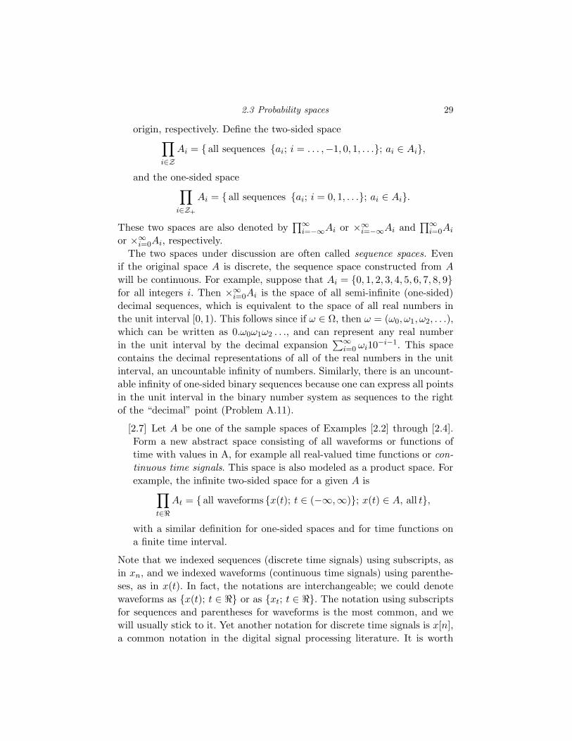
2.3 Probability spaces 29

origin, respectively. Define the two-sided space∏

i∈ZAi = all sequences ai; i = . . . ,−1, 0, 1, . . .; ai ∈ Ai,

and the one-sided space∏

i∈Z+

Ai = all sequences ai; i = 0, 1, . . .; ai ∈ Ai.

These two spaces are also denoted by∏∞

i=−∞Ai or ×∞i=−∞Ai and

∏∞i=0Ai

or ×∞i=0Ai, respectively.

The two spaces under discussion are often called sequence spaces. Even

if the original space A is discrete, the sequence space constructed from A

will be continuous. For example, suppose that Ai = 0, 1, 2, 3, 4, 5, 6, 7, 8, 9for all integers i. Then ×∞

i=0Ai is the space of all semi-infinite (one-sided)

decimal sequences, which is equivalent to the space of all real numbers in

the unit interval [0, 1). This follows since if ω ∈ Ω, then ω = (ω0, ω1, ω2, . . .),

which can be written as 0.ω0ω1ω2 . . ., and can represent any real number

in the unit interval by the decimal expansion∑∞

i=0 ωi10−i−1. This space

contains the decimal representations of all of the real numbers in the unit

interval, an uncountable infinity of numbers. Similarly, there is an uncount-

able infinity of one-sided binary sequences because one can express all points

in the unit interval in the binary number system as sequences to the right

of the “decimal” point (Problem A.11).

[2.7] Let A be one of the sample spaces of Examples [2.2] through [2.4].

Form a new abstract space consisting of all waveforms or functions of

time with values in A, for example all real-valued time functions or con-

tinuous time signals. This space is also modeled as a product space. For

example, the infinite two-sided space for a given A is∏

t∈ℜAt = all waveforms x(t); t ∈ (−∞,∞); x(t) ∈ A, all t,

with a similar definition for one-sided spaces and for time functions on

a finite time interval.

Note that we indexed sequences (discrete time signals) using subscripts, as

in xn, and we indexed waveforms (continuous time signals) using parenthe-

ses, as in x(t). In fact, the notations are interchangeable; we could denote

waveforms as x(t); t ∈ ℜ or as xt; t ∈ ℜ. The notation using subscripts

for sequences and parentheses for waveforms is the most common, and we

will usually stick to it. Yet another notation for discrete time signals is x[n],

a common notation in the digital signal processing literature. It is worth

30 Probability

remembering that vectors, sequences, and waveforms are all just indexed

collections of numbers; the only difference is the index set: finite for vectors,

countably infinite for sequences, and continuous for waveforms.

⋆ General product spaces All of the product spaces we have described can

be viewed as special cases of the general product space defined next.

Let I be an index set such as a finite set of integers Zk, the set of all

integers Z, the set of all nonnegative integers Z+, the real line ℜ, or the

nonnegative reals [0,∞). Given a family of spaces At; t ∈ I, define the

product space

AI =∏

t∈IAt = all at; t ∈ I; at ∈ At, all t.

The notation ×t∈IAt is also used for the same thing. Thus product spaces

model spaces of vectors, sequences, and waveforms whose coordinate values

are drawn from some fixed space. This leads to two notations for the space of

all k-dimensional vectors with coordinates in A : Ak and AZk . This shorter

and simpler notation is usually more convenient.

2.3.2 Event spaces

Intuitively, an event space is a collection of subsets of the sample space or

groupings of elementary events which we shall consider as physical events

and to which we wish to assign probabilities. Mathematically, an event space

is a collection of subsets that is closed under certain set-theoretic operations;

that is, performing certain operations on events or members of the event

space must give other events. Thus, for example, if in the example of a

single voltage measurement we have Ω = ℜ and we are told that the set of

all voltages greater than 5 volts, ω : ω ≥ 5, is an event, that is, it is a

member of a sigma-field F of subsets of ℜ, then necessarily its complement

ω : ω < 5 must also be an event, that is, a member of the sigma-field F .

If the latter set is not in F then F cannot be an event space! Observe that

no problem arises if the complement physically cannot happen – events that

“cannot occur” can be included in F and then assigned probability zero

when choosing the probability measure P . For example, even if you know

that the voltage does not exceed 5 volts, if you have chosen the real line

ℜ as your sample space, then you must include the set r : r > 5 in the

event space if the set r : r ≤ 5 is an event. The impossibility of a voltage

greater than 5 is then expressed by assigning P (r : r > 5) = 0.

2.3 Probability spaces 31

Although the definition of a sigma-field requires only that the class be

closed under complementation and countable unions, these requirements im-

mediately yield additional closure properties. The countably infinite version

of DeMorgan’s “laws” of elementary set theory (see Appendix A) requires

that if Fi, i = 1, 2, . . . , are all members of a sigma-field, then so is

∞⋂

i=1

Fi =

( ∞⋃

i=1

F ci

)c

.

It follows by similar set-theoretic arguments that any countable sequence

of any of the set-theoretic operations (union, intersection, complementa-

tion, difference, symmetric difference) performed on events must yield other

events. Observe, however, that there is no guarantee that uncountable opera-

tions on events will produce new events; they may or may not. For example,

if we are told that Fr; r ∈ [0, 1] is a family of events, then it is not neces-

sarily true that⋃

r∈[0,1]Fr, is an event (see Problem 2.3 for an example).

The requirement that a finite sequence of set-theoretic operations on

events yields other events is an intuitive necessity and is easy to verify for

a given collection of subsets of an abstract space: It is intuitively necessary

that logical combinations (and and or and not) of events corresponding to

physical phenomena should also be events to which a probability can be

assigned. If you know the probability of a voltage being greater than zero

and you know the probability that the voltage is not greater than 5 volts,

then you should also be able to determine the probability that the voltage is

greater than zero but not greater than 5 volts. It is easy to verify that finite

sequences of set-theoretic combinations yield events because the finiteness

of elementary set theory usually yields simple proofs.

A natural question arises in regard to (2.17) and (2.18): why not try to

construct a useful probability theory on the more general notion of a field

rather than a sigma-field? The response is that it unfortunately does not

work. Probability theory requires many results involving limits, and such

asymptotic results require the infinite relations of (2.19) and (2.25). In some

special cases, such as single coin flipping or single die rolling, the simpler

finite results suffice because there are only a finite number of possible out-

comes, and hence limiting results become trivial – any finite field is auto-

matically a sigma-field. If, however, one flips a coin forever, then there is

an uncountable infinity of possible outcomes, and the asymptotic relations

become necessary. Let Ω be the space of all one-sided binary sequences. Sup-

pose that you consider the smallest field formed by all finite set-theoretic

operations on the individual one-sided binary sequences, that is, on single-

32 Probability

ton sets in the sequence space. Then many countably infinite sets of binary

sequences (say the set of all periodic sequences) are not events since they

cannot be expressed as finite sequences of set-theoretic operations on the

singleton sets. Obviously, the sigma-field formed by including countable set-

theoretic operations does not have this defect. This is why sigma-fields must

be used rather than fields.

Limits of sets The condition (2.19) can be related to a condition on lim-

its by defining the notion of a limit of a sequence of sets. This notion will

prove useful when interpreting the axioms of probability. Consider a se-

quence Fn, n = 1, 2, . . ., of sets with the property that each set contains its

predecessor, that is, that Fn−1 ⊂ Fn for all n. Such a sequence of sets is said

to be nested and increasing. For example, the sequence Fn = [1, 2 − 1/n) of

subsets of the real line is increasing. The sequence (−n, a) is also increasing.

Intuitively, the first example increases to a limit of [1, 2) in the sense that

every point in the set [1, 2) is eventually included in one of the Fn. Similarly,

the sequence in the second example increases to (−∞, a). Formally, the limit

of an increasing sequence of sets can be defined as the union of all of the sets

in the sequence since the union contains all of the points in all of the sets in

the sequence and does not contain any points not contained in at least one

set (and hence an infinite number of sets) in the sequence:

limn→∞

Fn =∞⋃

n=1

Fn.

Figure 2.2(a) illustrates such a sequence in a Venn diagram. Thus the limit

of the sequence of sets [1, 2 − 1/n) is indeed the set [1, 2), as desired, and

the limit of (−n, a) is (∞, a). If F is the limit of a sequence of increasing

sets Fn, then we write Fn ↑ F .

Similarly, suppose that Fn, n = 1, 2, . . . is a decreasing sequence of nested

sets in the sense that Fn ⊂ Fn−1 for all n as illustrated by the Venn dia-

gram in Figure 2.2(b). For example, the sequences of sets [1, 1 + 1/n) and

(1 − 1/n, 1 + 1/n) are decreasing. Again we have a natural notion of the

limit of this sequence: both these sequences of sets collapse to the point of

singleton set 1 – the point in common to all the sets. This suggests a

formal definition based on the countably infinite intersection of the sets.

Given a decreasing sequence of sets Fn, n = 1, 2, . . . , we define the limit

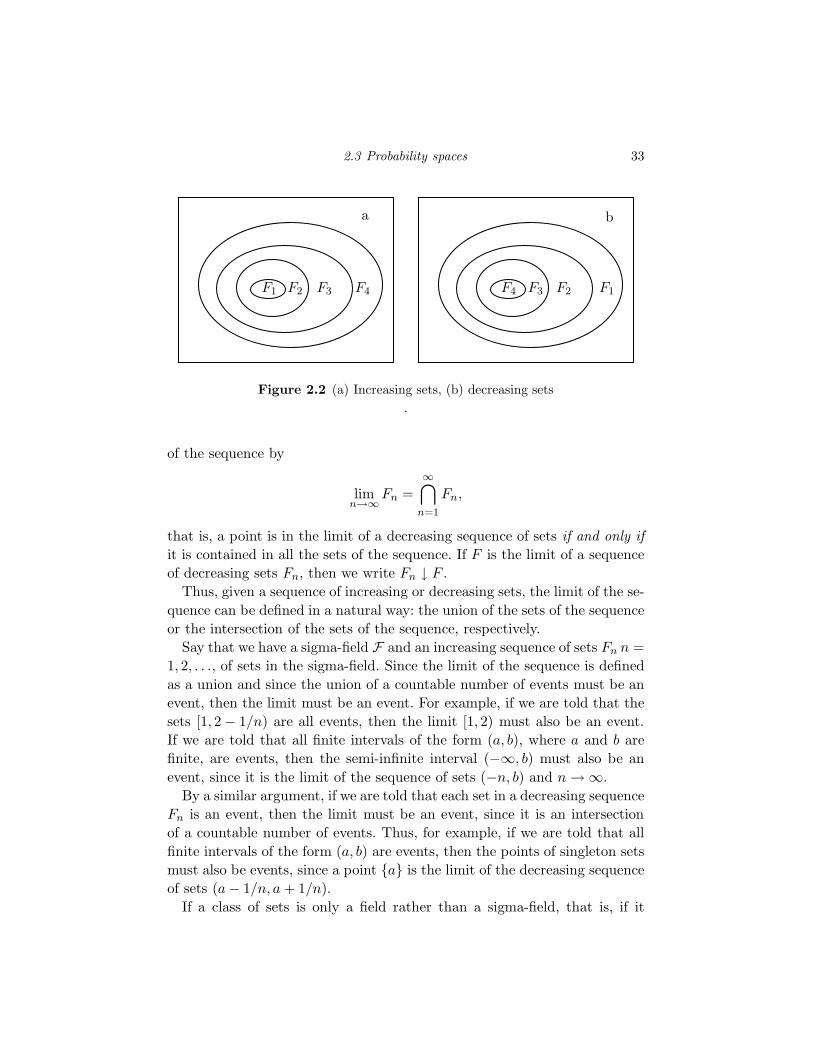
2.3 Probability spaces 33

a b

F1 F2 F3 F4 F4 F3 F2 F1

Figure 2.2 (a) Increasing sets, (b) decreasing sets

.

of the sequence by

limn→∞

Fn =

∞⋂

n=1

Fn,

that is, a point is in the limit of a decreasing sequence of sets if and only if

it is contained in all the sets of the sequence. If F is the limit of a sequence

of decreasing sets Fn, then we write Fn ↓ F .

Thus, given a sequence of increasing or decreasing sets, the limit of the se-

quence can be defined in a natural way: the union of the sets of the sequence

or the intersection of the sets of the sequence, respectively.

Say that we have a sigma-field F and an increasing sequence of sets Fn n =

1, 2, . . ., of sets in the sigma-field. Since the limit of the sequence is defined

as a union and since the union of a countable number of events must be an

event, then the limit must be an event. For example, if we are told that the

sets [1, 2 − 1/n) are all events, then the limit [1, 2) must also be an event.

If we are told that all finite intervals of the form (a, b), where a and b are

finite, are events, then the semi-infinite interval (−∞, b) must also be an

event, since it is the limit of the sequence of sets (−n, b) and n → ∞.

By a similar argument, if we are told that each set in a decreasing sequence

Fn is an event, then the limit must be an event, since it is an intersection

of a countable number of events. Thus, for example, if we are told that all

finite intervals of the form (a, b) are events, then the points of singleton sets

must also be events, since a point a is the limit of the decreasing sequence

of sets (a − 1/n, a + 1/n).

If a class of sets is only a field rather than a sigma-field, that is, if it

34 Probability

satisfies only (2.17) and (2.18), then there is no guarantee that the class will

contain all limits of sets. Hence, for example, knowing that a class of sets

contains all half-open intervals of the form (a, b] for a and b finite does not

ensure that it will also contain points or singleton sets! In fact, it is straight-

forward to show that the collection of all such half-open intervals together

with the complements of such sets and all finite unions of the intervals and

complements forms a field. The singleton sets, however, are not in the field!

(See Problem 2.6.)

Thus if we tried to construct a probability theory based on only a field,

we might have probabilities defined for events such as (a, b) meaning “the

output voltage of a measurement is between a and b” and yet not have

probabilities defined for a singleton set a meaning “the output voltage is

exactly a.” By requiring that the event space be a sigma-field instead of only

a field, we are assured that all such limits are indeed events.

It is a straightforward exercise to show that given (2.17) and (2.18), Prop-

erty (2.19) is equivalent to the following:

If Fn ∈ F ; n = 1, 2, . . . , is a decreasing sequence or an increasing sequence,

then

limn→∞

Fn ∈ F . (2.26)

We have already seen that (2.19) implies (2.26). For example, if (2.26) is

true and Gn is an arbitrary sequence of events, then define the increasing

sequence

Fn =

n⋃

i=1

Gi.

Obviously Fn−1 ⊂ Fn, and then (2.26) implies (2.19), since

∞⋃

i=1

Gi =

∞⋃

n=1

Fn = limn→∞

Fn ∈ F .

As we have noted, for a given sample space the selection of an event

space is not unique; it depends on the events to which it is desired to as-

sign probabilities and also on analytical limitations on the ability to assign

probabilities. We begin with two examples that represent the extremes of

event spaces – one possessing the minimum quantity of sets and the other

possessing the maximum. We then study event spaces useful for the sample

space examples of the preceding section.

2.3 Probability spaces 35

Examples

[2.8] Given a sample space Ω, then the collection Ω, ∅ is a sigma-field.

This is just the trivial event space already treated in Example [2.0].

Observe again that this is the smallest possible event space for any given

sample space because no other event space can have fewer elements.

[2.9] Given a sample space Ω, then the collection of all subsets of Ω is

a sigma-field. This is true since any countable sequence of set-theoretic

operations on subsets of Ω must yield another subset of Ω and hence

must be in the collection of all possible subsets. The collection of all

subsets of a space is called the power set of the space. Observe that this

is the largest possible event space for the given sample space, because it

contains every possible subset of the sample space.

This sigma-field is a useful event space for the sample spaces of Examples

[2.2] and [2.3], that is, for sample spaces that are discrete. We shall always

take our event space as the power set when dealing with a discrete sample

space (except possibly for a few perverse homework problems). A discrete

sample space with n elements has a power set with 2n elements (Problem

2.5). For example, the power set of the binary sample space Ω = 0, 1 is

the collection 0, 1,Ω = 0, 1, ∅, a list of all four possible subsets of

the space.

Unfortunately, the power set is too large to be useful for continuous spaces.

To treat the reasons for this is beyond the scope of a book at this level, but we

can say that it is not possible in general to construct interesting probability

measures on the power set of a continuous space. There are special cases

where we can construct particular probability measures on the power set of

a continuous space by mimicking the construction for a discrete space (see,

e.g., Problems 2.5, 2.7, and 2.10). Truly continuous experiments cannot,

however, be rigorously defined for such a large event space because integrals

cannot be defined over all events in such spaces.

Although both of the preceding examples can be used to provide event

spaces for the special case of Ω = ℜ, the real line, neither leads to a useful

probability theory in that case. In the next example we consider another

event space for the real line that is more useful and, in fact, is used almost

always for ℜ and higher-dimensional Euclidean spaces. First, however, we

need to treat the idea of generating an event space from a collection of

important events. Intuitively, given a collection of important sets G that we

require to be events, the event space σ(G) generated by G is the smallest

event space F to which all the sets in G belong. That is, σ(G) is an event

36 Probability

space, it contains all the sets in G, and no smaller collection of sets satisfies

these two conditions.

Regardless of the details, it is worth emphasizing the key points of this

discussion.

• The notion of a generated sigma-field allows one to describe an event space for

the real line, called the Borel field, that contains all physically important events

and that will lead to a useful calculus of probability. It is usually not important

to understand the detailed structure of this event space past the facts that it

– is indeed an event space, and

– contains all the important events such as intervals .

• The notion of a generated sigma-field can be used to extend the event space of

the real line to event spaces of vectors, sequences, and waveforms taking on real

values. Again the detailed structure is usually not important past the fact that it

– is indeed an event space, and

– contains all the important events such as those described by requiring any finite

collection of coordinate values to lie within intervals.

⋆Generating event spaces Any useful event space for the real line should

include as members all intervals of the form (a, b) since we certainly wish to

consider events of the form “the output voltage is between 3 and 5 volts.”

Furthermore, we obviously require it satisfy the defining properties for an

event space; that is, require a collection of subsets of Ω that satisfy Properties

(2.17) through (2.19). A means of accomplishing both of these goals in a

relatively simple fashion is to define our event space as the smallest sigma-

field that contains the desired subsets, to wit, the intervals and all of their

countable set-theoretic combinations (bewildering as it may seem, this is not

the same as all subsets of ℜ). Of course, although a sigma-field that is based

on the intervals is most useful, it is also possible to consider other starting

points. These considerations motivate the following general definition.

Given a sample space Ω (such as the real line ℜ) and an arbitrary class

G of subsets of Ω – usually the class of all open intervals of the form (a, b)

when Ω = ℜ – define σ(G), the sigma-field generated by the class G, to be

the smallest sigma-field containing all of the sets in G, where by “smallest”

we mean that if F is any sigma-field and it contains G, then it contains σ(G).

(See any book on measure theory, e.g. [1].)

For example, as noted before, we might require that a sigma-field of the

real line contain all intervals; then it would also have to contain at least

all complements of intervals and all countable unions and intersections of

intervals and all countable complements, unions, and intersections of these

2.3 Probability spaces 37

results, ad infinitum. This technique will be used several times to spec-

ify useful event spaces in complicated situations such as continuous simple

spaces, sequence spaces, and function spaces. We are now ready to provide

the proper, most useful event space for the real line.

[2.10] Given the real line ℜ, the Borel field (or, more accurately, the Borel

sigma-field) is defined as the sigma-field generated by all the open inter-

vals of the form (a, b). The members of the Borel field are called Borel

sets. We shall denote the Borel field by B(ℜ), and hence

B(ℜ) = σ (all open intervals).

Since B(ℜ) is a sigma-field and since it contains all of the open intervals, it

must also consider limit sets of the form

(−∞, b) = limn→∞

(−n, b) ,

(a,∞) = limn→∞

(a, n) ,

and

a = limn→∞

(a − 1/n, a + 1/n),

that is, the Borel field must include semi-infinite open intervals and the

singleton sets or individual points. Furthermore, since the Borel field is a

sigma-field it must contain differences. Hence it must contain semi-infinite

half-open sets of the form

(−∞, b] = (−∞,∞) − (b,∞),

and since it must contain unions of its members, it must contain half-open

intervals of the form

(a, b] = (a, b) ∪ b and [a, b) = (a, b) ∪ a.In addition, it must contain all closed intervals and all finite or countable

unions and complements of intervals of any of the preceding forms. Roughly

speaking, the Borel field contains all subsets of the real line that can be

constructed by countable sequences of operations on intervals. It is a deep

and difficult result of measure theory that the Borel field of the real line

is in fact different from the power set of the real line; that is, there exist

subsets of the real line that are not in the Borel field. Although we will not

describe such a subset, we can guarantee that these “unmeasurable” sets

have no physical importance, that they are very hard to construct, and that

an engineer will never encounter such a subset in practice. It may, however,

be necessary to demonstrate that some weird subset is in fact an event in

38 Probability

this sigma-field. This is typically accomplished by showing that it is the limit

of simple Borel sets.

In some cases we wish to deal not with a sample space that is the entire

real line, but with one that is some subset of the real line. In this case we

define the Borel field as the Borel field of the real line “cut down” to the

smaller space.

Given that the sample space, Ω, is a Borel subset of the real line ℜ, the

Borel field of Ω, denoted B(Ω), is defined as the collection of all sets of the

form F ∩ Ω, for F ∈ B(ℜ); that is, the intersection of Ω with all of the Borel

sets of ℜ forms the class of Borel sets of Ω.

It can be shown (Problem 2.4) that, given a discrete subset A of the real

line, the Borel field B(A) is identical to the power set of A. Thus, for the

first three examples of sample spaces, the Borel field serves as a useful event

space since it reduces to the intuitively appealing class of all subsets of the

sample space.

The remaining examples of sample spaces are all product spaces. The con-

struction of event spaces for such product spaces – that is, spaces of vectors,

sequences, or waveforms – is more complicated and less intuitive than the

constructions for the preceding event spaces. In fact, there are several pos-

sible techniques of construction, which in some cases lead to different event

spaces. We wish to convey an understanding of the structure of such event

spaces, but we do not wish to dwell on the technical difficulties that can be

encountered. Hence we shall study only one of the possible constructions –

the simplest possible definition of a product sigma-field – by making a di-

rect analogy to a product sample space. This definition will suffice for most

systems studied herein, but it has shortcomings. At this time we mention

one particular weakness: the event space that we shall define may not be big

enough when studying the theory of continuous time random processes.

[2.11] Given an abstract space A, a sigma-field F of subsets of A, an index

set I, and a product sample space of the form

AI =∏

t∈IAt,

where the At are all replicas of A, the product sigma-field

FI =∏

t∈IFt,

is defined as the sigma-field generated by all “one-dimensional” sets of

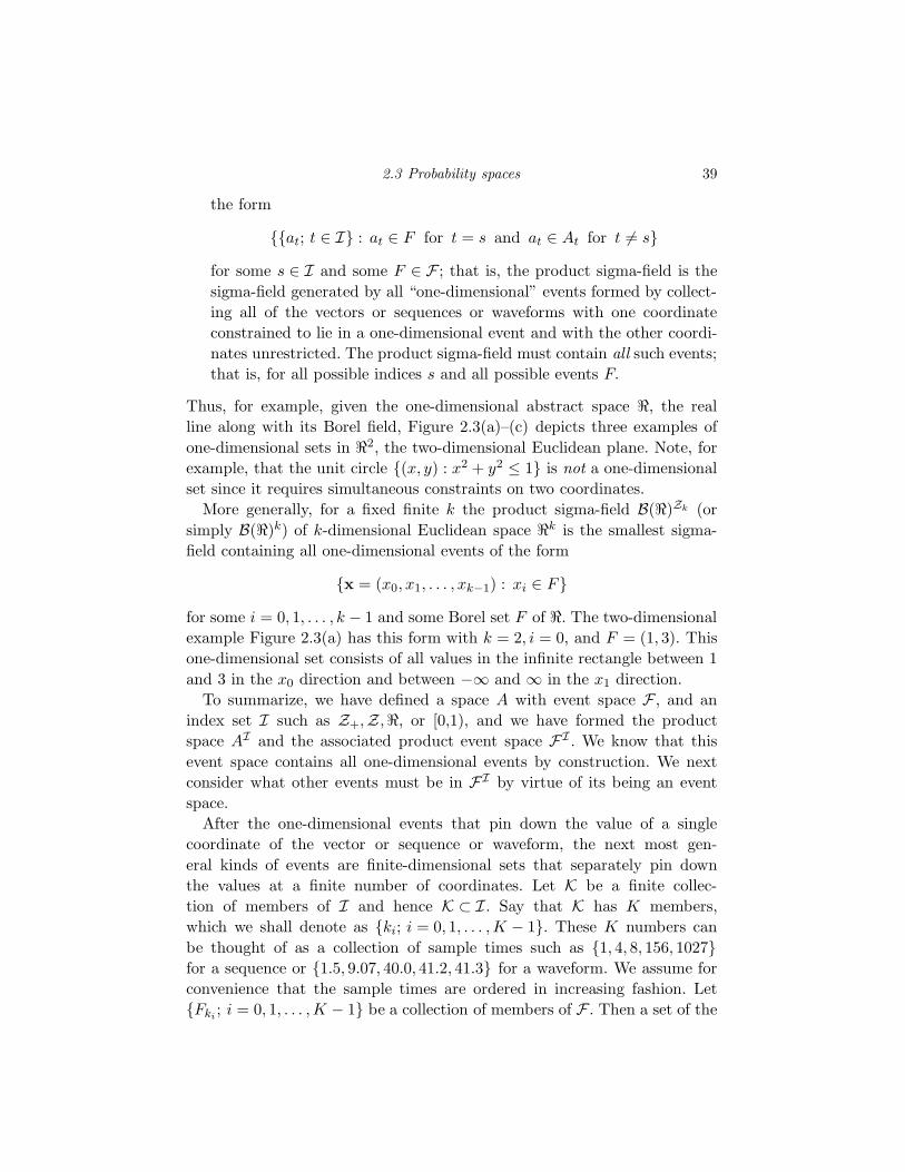
2.3 Probability spaces 39

the form

at; t ∈ I : at ∈ F for t = s and at ∈ At for t 6= s

for some s ∈ I and some F ∈ F ; that is, the product sigma-field is the

sigma-field generated by all “one-dimensional” events formed by collect-

ing all of the vectors or sequences or waveforms with one coordinate

constrained to lie in a one-dimensional event and with the other coordi-

nates unrestricted. The product sigma-field must contain all such events;

that is, for all possible indices s and all possible events F.

Thus, for example, given the one-dimensional abstract space ℜ, the real

line along with its Borel field, Figure 2.3(a)–(c) depicts three examples of

one-dimensional sets in ℜ2, the two-dimensional Euclidean plane. Note, for

example, that the unit circle (x, y) : x2 + y2 ≤ 1 is not a one-dimensional

set since it requires simultaneous constraints on two coordinates.

More generally, for a fixed finite k the product sigma-field B(ℜ)Zk (or

simply B(ℜ)k) of k-dimensional Euclidean space ℜk is the smallest sigma-

field containing all one-dimensional events of the form

x = (x0, x1, . . . , xk−1) : xi ∈ F

for some i = 0, 1, . . . , k − 1 and some Borel set F of ℜ. The two-dimensional

example Figure 2.3(a) has this form with k = 2, i = 0, and F = (1, 3). This

one-dimensional set consists of all values in the infinite rectangle between 1

and 3 in the x0 direction and between −∞ and ∞ in the x1 direction.

To summarize, we have defined a space A with event space F , and an

index set I such as Z+,Z,ℜ, or [0,1), and we have formed the product

space AI and the associated product event space FI . We know that this

event space contains all one-dimensional events by construction. We next

consider what other events must be in FI by virtue of its being an event

space.

After the one-dimensional events that pin down the value of a single

coordinate of the vector or sequence or waveform, the next most gen-

eral kinds of events are finite-dimensional sets that separately pin down

the values at a finite number of coordinates. Let K be a finite collec-

tion of members of I and hence K ⊂ I. Say that K has K members,

which we shall denote as ki; i = 0, 1, . . . ,K − 1. These K numbers can

be thought of as a collection of sample times such as 1, 4, 8, 156, 1027for a sequence or 1.5, 9.07, 40.0, 41.2, 41.3 for a waveform. We assume for

convenience that the sample times are ordered in increasing fashion. Let

Fki; i = 0, 1, . . . ,K − 1 be a collection of members of F . Then a set of the

40 Probability

a b

c d

Figure 2.3 One-dimensional (a)–(c) and two-dimensionalevents (d) in two-dimensional space. (a)(x0, x1) : x0 ∈ (1, 3),(b)(x0, x1) : x1 ∈ (3, 6), (c)(x0, x1) : x1 ∈ (4, 5) ∪ (−∞,−2),(d)(x0, x1) : x0 ∈ (1, 3); x1 ∈ (3, 6).

form xt; t ∈ I : xki∈ Fki

; i = 0, 1, . . . ,K − 1 is an example of a finite-

dimensional set. Note that it collects all sequences or waveforms such that a

finite number of coordinates are constrained to lie in one-dimensional events.

An example of two-dimensional sets of this form in two-dimensional space

is illustrated in Figure 2.3(d). Observe that when the one-dimensional sets

constraining the coordinates are intervals, then the two-dimensional sets are

rectangles. Analogous to the two-dimensional example, finite-dimensional

events having separate constraints on each coordinate are called rectangles.

Observe, for example, that a circle or sphere in Euclidean space is not a

rectangle because it cannot be defined using separate constraints on the co-

ordinates; the constraints on each coordinate depend on the values of the

2.3 Probability spaces 41

others – e.g., in two dimensions for a circle of radius one we require that

x20 ≤ 1 − x2

1.

Note that Figure 2.3(d) is just the intersection of examples (a) and (b)

of Figure 2.3. In general we can express finite-dimensional rectangles as

intersections of one-dimensional events as follows

xt; t ∈ I : xki∈ Fki

; i = 0, 1, . . . ,K − 1 =

K−1⋂

i=0

xt; t ∈ I : xki∈ Fi,

that is, a set constraining a finite number of coordinates to each lie in one-

dimensional events or sets in F is the intersection of a collection of one-

dimensional events. Since FI is a sigma-field and since it contains the one-

dimensional events, it must contain such finite intersections, and hence it

must contain such finite-dimensional events.

By concentrating on events that can be represented as the finite inter-

section of one-dimensional events we do not mean to imply that all events

in the product event space can be represented in this fashion – the event

space will also contain all possible limits of finite unions of such rectangles,

complements of such sets, and so on. For example, the unit circle in two

dimensions is not a rectangle, but it can be considered as a limit of unions

of rectangles and hence is in the event space generated by the rectangles.

(See Problem 2.36.)

The moral of this discussion is that the product sigma-field for spaces of

sequences and waveforms must contain (but not consist exclusively of) all

sets that are described by requiring that the outputs of coordinates for a

finite number of events lie in sets in the one-dimensional event space F .

We shall further explore such product event spaces when considering ran-

dom processes, but the key points remain:

1. a product event space is a sigma-field

2. it contains all “one-dimensional events” consisting of subsets of the product

sample space formed by grouping together all vectors or sequences or waveforms

having a single fixed coordinate lying in a one-dimensional event. In addition,

it contains all rectangles or finite-dimensional events consisting of all vectors or

sequences or waveforms having a finite number of coordinates constrained to lie

in one-dimensional events.

2.3.3 Probability measures

The defining axioms of a probability measure as given in equations (2.22)

through (2.25) correspond generally to intuitive notions, at least for the first

42 Probability

three properties. The first property requires that a probability be a nonnega-

tive number. In a purely mathematical sense, this is an arbitrary restriction,

but it is in accord with the long history of intuitive and combinatorial devel-

opments of probability. Probability measures share this property with other

measures such as area, volume, weight, and mass.

The second defining property corresponds to the notion that the proba-

bility that something will happen or that an experiment will produce one

of its possible outcomes is one. This, too, is mathematically arbitrary but

is a convenient and historical assumption. (From childhood we learn about

things that are “100% certain” – obviously we could as easily take 1 or π

(but not infinity – why?) to represent certainty.)

The third property, “additivity” or “finite additivity,” is the key one. In

English it reads that the probability of occurrence of a finite collection of

events having no points in common must be the sum of the probabilities of

the separate events. More generally, the basic assumption of measure the-

ory is that any measure – probabilistic or not – such as weight, volume,

mass, and area should be additive: the mass of a group of disjoint regions of

matter should be the sum of the separate masses; the weight of a group of

objects should be the sum of the individual weights. Equation (2.24) only

pins down this property for finite collections of events. The additional re-

striction of (2.25), called countable additivity, is a limiting or asymptotic

or infinite version, analogous to (2.19) for set algebra. This again leads to

the rhetorical questions of why the more complicated, more restrictive, and

less intuitive infinite version is required. In fact, it was the addition of this

limiting property that provided the fundamental idea for Kolmogorov’s de-

velopment of modern probability theory in the 1930s.

The response to the rhetorical question is essentially the same as that

for the asymptotic set algebra property: countably infinite properties are

required to handle asymptotic and limiting results. Such results are crucial

because we often need to evaluate the probabilities of complicated events

that can only be represented as a limit of simple events. (This is analogous

to the way that integrals are obtained as limits of finite sums.)

Note that it is countable additivity that is required. Uncountable addi-

tivity cannot be defined sensibly. This is easily seen in terms of the fair

wheel mentioned at the beginning of the chapter. If the wheel is spun, any

particular number has probability zero. On the other hand, the probability

of the event made up of all of the uncountable numbers between 0 and 1

is obviously one. If you consider defining the probability of all the numbers

2.3 Probability spaces 43

between 0 and 1 to be the uncountable sum of the individual probabilities,

you see immediately the essential contradiction that results.

Since countable additivity has been added to the axioms proposed in

the introduction, the formula (2.11) used to compute probabilities of events

broken up by a partition immediately extends to partitions with a countable

number of elements; that is, if Fk, k = 1, 2, . . ., forms a partition of Ω into

disjoint events (Fn ∩ Fk = ∅ if n 6= k and⋃

k Fk = Ω), then for any event G

P (G) =

∞∑

k=1

P (G ∩ Fk). (2.27)

Limits of probabilities At times we are interested in finding the probability of

the limit of a sequence of events. To relate the countable additivity property

of (2.25) to limiting properties, recall the discussion of the limiting properties

of events given earlier in this chapter in terms of increasing and decreasing

sequences of events. Say we have an increasing sequence of events Fn, n =

0, 1, 2, . . . , Fn−1 ⊂ Fn, and let F denote the limit set, that is, the union of

all of the Fn. We have already argued that the limit set F is itself an event.

Intuitively, since the Fn converge to F , the probabilities of the Fn should

converge to the probability of F. Such convergence is called a continuity

property of probability and is very useful for evaluating the probabilities

of complicated events as the limit of a sequence of probabilities of simpler

events. We shall show that countable additivity implies such continuity. To

accomplish this, define the sequence of sets G0 = F0 and Gn = Fn − Fn−1

for n = 1, 2, . . . The Gn are disjoint and have the same union as do the Fn

(see Figure 2.2(a) as a visual aid). Thus we have from countable additivity

that

P(

limn→∞

Fn

)= P

( ∞⋃

k=0

Fk

)

= P

( ∞⋃

k=0

Gk

)

=∞∑

k=0

P (Gk) = limn→∞

n∑

k=0

P (Gk),

where the last step simply uses the definition of an infinite sum. Since Gn =

Fn − Fn−1 and Fn−1 ⊂ Fn, P (Gn) = P (Fn) − P (Fn−1) and hence

n∑

k=0

P (Gk) = P (F0) +

n∑

k=1

(P (Fn) − P (Fn−1)) = P (Fn).

This is an example of what is called a “telescoping sum” where each term

44 Probability

cancels the previous term and adds a new piece, i.e.,

P (Fn) = + P (Fn) − P (Fn−1)

+ P (Fn−1) − P (Fn−2)

+ P (Fn−2) − P (Fn−3)

...

+ P (F1) − P (F0)

+ P (F0).

Combining these results completes the proof of the following statement.If Fn is a sequence of increasing events, then

P(

limn→∞

Fn

)= lim

n→∞P (Fn), (2.28)

that is, the probability of the limit of a sequence of increasingevents is the limit of the probabilities.

Note that the sequence of probabilities on the right-hand side of (2.28) is

increasing with increasing n. Thus, for example, probabilities of semi-infinite

intervals can be found as a limit as P ((−∞, a]) = limn→∞ P ((−n, a]). A

similar argument can be used to show that one can also interchange the

limit with the probability measure given a sequence of decreasing events;

that is,If Fn is a sequence of decreasing events, then

P(

limn→∞

Fn

)= lim

n→∞P (Fn). (2.29)

that is, the probability of the limit of a sequence of decreasingevents is the limit of the probabilities.

Note that the sequence of probabilities on the right-hand side of (2.29) is

decreasing with increasing n. Thus, for example, the probabilities of points

can be found as a limit of probabilities of intervals, P (a) = limn→∞ P ((a −1/n, a + 1/n)).

It can be shown (see Problem 2.21) that, given (2.22) through (2.24), the

three conditions (2.25), (2.28), and (2.29) are equivalent; that is, any of the

three could serve as the fourth axiom of probability.

Property (2.28) is called continuity from below, and (2.29) is called conti-

nuity from above. The designations “from below” and “from above” relate to

the direction from which the respective sequences of probabilities approach

their limit. These continuity results are the basis for using integral calculus

to compute probabilities, since integrals can be expressed as limits of sums.

2.4 Discrete probability spaces 45

2.4 Discrete probability spaces

We now provide several examples of probability measures on our examples

of sample spaces and sigma-fields and thereby give complete examples of

probability spaces.

The first example formalizes the description of a probability measure as

a sum of a pmf as first mentioned in the introductory section.

[2.12] Let Ω be a finite set and let F be the power set of Ω. Suppose that

we have a function p(ω) that assigns a real number to each sample point

ω in such a way that

p(ω) ≥ 0, all ω ∈ Ω (2.30)

and∑

ω∈Ω

p(ω) = 1. (2.31)

Define the set function P by

P (F ) =∑

ω∈F

p(ω) =∑

ω∈Ω

1F (ω)p(ω), all F ∈ F (2.32)

where 1F (ω) is the indicator function of the set F , 1 if ω ∈ F and 0

otherwise.

For simplicity we drop the ω ∈ Ω underneath the sum; that is, when no range

of summation is explicit, it should be assumed the sum is over all possible

values. Thus we can abbreviate (2.32) to

P (F ) =∑

1F (ω)p(ω), all F ∈ F . (2.33)

The set function P is easily verified to be a probability measure: it obviously

satisfies Axioms 2.1 and 2.2. It is finitely and countably additive from the

properties of sums. In particular, given a sequence of disjoint events, only a

finite number can be distinct (since the power set of a finite space has only

a finite number of members). To be disjoint, the balance of the sequence

must equal ∅. The probability of the union of these sets will be the finite

sum of the p(ω) over the points in the union. This equals the sum of the

probabilities of the sets in the sequence. Example [2.1] is a special case of

Example [2.12], as is the coin flip example of the introductory section.

A function p(ω) satisfying (2.30) and (2.31) is called a probability mass

function or pmf. Analogous to a positive-valued point mass function in

physics which is summed to find a total mass in a volume, the pmf is summed

over region to find the probability of that region.

46 Probability

Expectations

The summation (2.33) used to define probability measures for a discrete

space is a special case of a more general weighted sum, which we pause to

define and consider. Suppose that g is a real-valued function defined on Ω,

i.e., g : Ω → ℜ assigns a real number g(ω) to every ω ∈ Ω. We could consider

more general complex-valued functions, but for the moment it is simpler to

stick to real-valued functions. Also, we could consider mappings of Ω into

subsets of ℜ, but it is convenient for the moment to let the range of g be

the entire real line. Recall that in the introductory section we considered

such a function to be an example of signal processing and called it a random

variable. Given a pmf p, define the expectation of g (with respect to p) as 21

E(g) =∑

g(ω)p(ω). (2.34)

With this definition, (2.33) with g(ω) = 1F (ω) yields

P (F ) = E(1F ), (2.35)

showing that the probability of an event is the expectation of the indicator

function of the event. Mathematically, we can think of expectation as a

generalization of the idea of probability since probability is the special case

of expectation that results when the only functions allowed are indicator

functions.

Expectations are also called probabilistic averages or statistical averages.

For the time being, probabilities are the most important examples of expec-

tation. We shall see many examples, however, so it is worthwhile to mention

a few of the most important. Suppose that the sample space is a subset of the

real line, e.g., Z or Zn. One of the most commonly encountered expectations

is the mean or first moment

m =∑

ωp(ω), (2.36)

where g(ω) = ω, the identity function. A more general idea is the kth mo-

ment defined by

m(k) =∑

(ω)kp(ω), (2.37)

so that m = m(1). After the mean, the most commonly encountered moment

1 This is not in fact the fundamental definition of expectation that will be intro-duced in Chapter 4, but it will be seen to be equivalent.

2.4 Discrete probability spaces 47

in practice is the second moment,

m(2) =∑

(ω)2p(ω). (2.38)

Moments can be thought of as parameters describing a pmf, and some com-

putations involving signal processing will turn out to depend only on certain

moments.

A slight variation on kth (or kth order) moments is the so-called central-

ized moment formed by subtracting the mean before taking the power:∑

(ω − m)kp(ω), (2.39)

but the only such moment commonly encountered in practice is the variance

σ2 =∑

(ω − m)2p(ω). (2.40)

The variance and the second moment are easily related as

σ2 =∑

(ω − m)2p(ω)

=∑

(ω2 − 2ωm + m2)p(ω)

=∑

ω2p(ω) − 2m∑

ωp(ω) + m2∑

p(ω)

= m(2) − 2m2 + m2 = m(2) − m2. (2.41)

Probability mass functions

It is important to observe that the probability mass function is defined

only for points in the sample space, whereas a probability measure is defined

for events, sets which belong to an event space. Intuitively, the probability

of a set is given by the sum of the probabilities of the points as given by

the pmf. Obviously it is much easier to describe the probability function

than the probability measure since it need only be specified for points. The

axioms of probability then guarantee that the probability function can be

used to compute the probability measure. Note that given one probability

form, we can always determine the other. In particular, given the pmf p, we

can construct P using (2.32). Given P , we can find the corresponding pmf

p from the formula

p(ω) = P (ω).

We list below several of the most common examples of pmf’s. The reader

should verify that they are all indeed valid pmf’s, that is, that they satisfy

48 Probability

(2.30) and (2.31).

The binary pmf. Ω = 0, 1; p(0) = 1 − p, p(1) = p, where p is a parame-

ter in (0, 1).

A uniform pmf. Ω = Zn = 0, 1, . . . , n − 1 and p(k) = 1/n; k ∈ Zn.

The binomial pmf. Ω = Zn+1 = 0, 1, . . . , n and

p(k) =

(n

k

)pk(1 − p)n−k; k ∈ Zn+1,

where(

n

k

)=

n!

k!(n − k)!

is the binomial coefficient (read as “n choose k”).

The binary pmf is a probability model for coin flipping with a biased coin

or for a single sample of a binary data stream. A uniform pmf on Z6 can

model the roll of a fair die. Observe that it would not be a good model

for ASCII data since, for example, the letters t and e and the symbol for

space have a higher probability than other letters. The binomial pmf is a

probability model for the number of heads in n successive independent flips

of a biased coin, as will later be seen.

The same construction provides a probability measure on countably infi-

nite spaces such as Z and Z+. It is no longer as simple to prove countable

additivity, but it should be fairly obvious that it holds and, at any rate, it

follows from standard results in elementary analysis for convergent series.

Hence we shall only state the following example without proving countable

additivity, but bear in mind that it follows from the properties of infinite

summations.

[2.13] Let Ω be a space with a countably infinite number of elements and

let F be the power set of Ω. Then if p(ω); ω ∈ Ω satisfies (2.30) and

(2.31), the set function P defined by (2.32) is a probability measure.

Two common examples of pmf’s on countably infinite sample spaces follow.

The reader should test their validity.

The geometric pmf. Ω = 1, 2, 3, . . . and p(k) = (1 − p)k−1p; k =

1, 2, . . ., where p ∈ (0, 1) is a parameter.

2.4 Discrete probability spaces 49

The Poisson pmf. Ω = Z+ = 0, 1, 2, . . . and p(k) = (λke−λ)/k!, where

λ is a parameter in (0,∞). (Keep in mind that 0!∆= 1.)

We will later see the origins of several of these pmf’s and their applications.

For example, both the binomial and the geometric pmf will be derived from

the simple binary pmf model for flipping a single coin. For the moment they

should be considered as common important examples. Various properties of

these pmf’s and a variety of calculations involving them are explored in the

problems at the end of the chapter.

Computational examples

The various named pmf’s provide examples for computing probabilities

and other expectations. Although much of this is prerequisite material, it

does not hurt to collect several of the more useful tricks that arise in evaluat-

ing sums. The binary pmf on its own is too simple to provide much interest,

so first consider the uniform pmf on Zn. This is trivially a valid pmf since

it is nonnegative and sums to 1. The probability of any set is simply

P (F ) =1

n

∑1F (ω) =

#(F )

n,

where #(F ) denotes the number of elements or points in the set F . The

mean is given by

m =1

n

n−1∑

k=0

k =n + 1

2, (2.42)

a standard formula easily verified by induction, as detailed in Appendix B.

The second moment is given by

m(2) =1

n

1

n

n−1∑

k=0

k2 =(n + 1)(2n + 1)

6, (2.43)

as can also be verified by induction. The variance can be found by combining

(2.43), (2.42), and (2.41).

The binomial pmf is more complicated. The first issue is to prove that it

sums to one and hence is a valid pmf (it is obviously nonnegative). This is

50 Probability

accomplished by recalling the binomial theorem from high-school algebra:

(a + b)n =

n∑

k=0

(n

k

)anbn−k (2.44)

and setting a = p and b = 1 − p to write

n∑

k=0

p(k) =

n∑

k=0

(n

k

)pk(1 − p)n−k

= (p + 1 − p)n = 1.

Finding moments is trickier here, and we shall later develop a much easier

way to do this using exponential transforms. Nonetheless, it provides useful

practice to compute an example sum, if only to demonstrate later how much

work can be avoided! Finding the mean requires evaluation of the sum

m =

n∑

k=0

k

(n

k

)pk(1 − p)n−k

=

n∑

k=1

n!

(n − k)!(k − 1)!pk(1 − p)n−k.

The trick here is to recognize that the sum looks very much like the terms in

the binomial theorem, but a change of variables is needed to get the binomial

theorem to simplify things. Changing variables by defining l = k − 1, the

sum becomes

m =

n−1∑

l=0

n!

(n − l − 1)!l!pl+1(1 − p)n−l−1,

which will very much resemble the binomial theorem with n − 1 replacing n

if we factor out a p and an n:

m = np

n−1∑

l=0

(n − 1)!

(n − 1 − l)!l!pl(1 − p)n−1−l

= np(p + 1 − p)n−1 = np. (2.45)

The second moment is messier, so its evaluation is postponed until simpler

means are developed.

The geometric pmf is handled using the geometric progression, usually

treated in high-school algebra and summarized in Appendix B. From (B.4)

2.4 Discrete probability spaces 51

in Appendix B we have for any real a with |a| < 1

∞∑

k=0

ak =1

1 − a, (2.46)

which proves that the geometric pmf indeed sums to 1.

Evaluation of the mean of the geometric pmf requires evaluation of the

sum

m =∞∑

k=1

kp(k) =∞∑

k=1

kp(1 − p)k−1.

One may have access to a book of tables which includes this sum, but a

useful trick can be used to evaluate the sum from the well-known result

for summing a geometric series. The trick involves differentiating the usual

geometric progression sum, as detailed in Appendix B, where it is shown for

any q ∈ (0, 1) that

∞∑

k=0

kqk−1 =1

(1 − q)2. (2.47)

Set q = 1 − p in (2.47) and the formula for m yields

m =1

p. (2.48)

A similar idea works for the second moment. From (B.7) of Appendix B the

second moment is given by

m(2) =

∞∑

k=1

k2p(1 − p)k−1 = p

(2

p3− 1

p2

)(2.49)

and hence from (2.41) the variance is

σ2 =2

p2. (2.50)

As an example of a probability computation using a geometric pmf, sup-

pose that (Ω,F , P ) is a discrete probability space with Ω = Z+, F the

power set of Ω, and P the probability measure induced by the geometric

pmf with parameter p. Find the probabilities of the event F = k : k ≥ 10and G = k : k is odd. Alternatively note that F = 10, 11, 12, . . . and

G = 1, 3, 5, 7, . . . (we consider only odd numbers in the sample space, that

52 Probability

is, only positive odd numbers). We have that

P (F ) =∑

k∈F

p(k) =

∞∑

k=10

p(1 − p)k−1

=p

1 − p

∞∑

k=10

(1 − p)k =p

1 − p(1 − p)10

∞∑

k=10

(1 − p)k−10

= p(1 − p)9∞∑

k=0

(1 − p)k = (1 − p)9,

where the suitable form of the geometric progression has been derived from

the basic form (B.4). Although we have concentrated on the calculus, this

problem could be interpreted as a solution to a word problem. For example,

suppose you arrive at the post office and you know that the probability of

k people being in line is a geometric distribution with p = 1/2. What is the

probability that there are at least ten people in line? From the solution just

obtained the answer is (1 − 0.5)9 = 2−9.

To find the probability of an odd outcome, we proceed in the same general

fashion to write

P (G) =∑

k∈G

p(k) =∑

k=1,3,...

p(1 − p)k−1

= p∑

k=0,2,4,...

(1 − p)k = p

∞∑

k=0

[(1 − p)2]k

=p

1 − (1 − p)2=

1

2 − p.

Thus in the English example of the post office lines, the probability of finding

an odd number of people in line is 2/3.

Lastly we consider the Poisson pmf, again beginning with a verification

that it is indeed a pmf. Consider the sum

∞∑

k=0

p(k) =

∞∑

k=0

λke−λ

k!= e−λ

∞∑

k=0

λk

k!.

Here the trick is to recognize the sum as the Taylor series expansion for an

exponential, that is,

eλ =∞∑

k=0

λk

k!,

2.4 Discrete probability spaces 53

whence

∞∑

k=0

p(k) = e−λeλ = 1,

proving the claim.

To evaluate the mean of the Poisson pmf, begin with

∞∑

k=0

kp(k) =

∞∑

k=1

kλke−λ

k!= e−λ

∞∑

k=1

λk

(k − 1)!.

Change variables l = k − 1 and pull a λ out of the sum to write

∞∑

k=0

kp(k) = λe−λ∞∑

l=0

λl

l!.

Recognizing the sum as eλ, this yields

m = λ. (2.51)

The second moment is found similarly, but with more bookkeeping. Analo-

gous to the mean computation,

m(2) =

∞∑

k=1

k2 λke−λ

k!=

∞∑

k=2

k(k − 1)λke−λ

k!+ m

=∞∑

k=2

λke−λ

(k − 2)!+ m.

Change variables l = k − 2 and pull λ2 out of the sum to obtain

m(2) = λ2∞∑

l=0

λle−λ

l!+ m = λ2 + λ (2.52)

so that from (2.41) the variance is

σ2 = λ. (2.53)

Multidimensional pmf’s

Although the foregoing ideas were developed for scalar sample spaces such

as Z+, they also apply to vector sample spaces. For example, if A is a discrete

space, then so is the vector space Ak = all vectors x = (x0, . . . xk−1) with

54 Probability

xi ∈ A, i = 0, 1, . . . , k − 1. A common example of a pmf on vectors is the

product pmf considered next.

[2.14] The product pmf.

Let pi; i = 0, 1, . . . , k − 1, be a collection of one-dimensional pmf’s;

that is, for each i = 0, 1, . . . , k − 1 pi(r); r ∈ A satisfies (2.30) and (2.31).

Define the product k-dimensional pmf p on Ak by

p(x) = p(x0, x1, . . . , xk−1) =k−1∏

i=0

pi(xi).

As a more specific example, suppose that all of the marginal pmf’s are

the same and are given by a Bernoulli pmf:

p(x) = px(1 − p)1−x; x = 0, 1.

Then the corresponding product pmf for a k-dimensional vector becomes

p(x0, x1, . . . , xk−1) =

k−1∏

i=0

pxi(1 − p)1−xi

= pw(x0,x1,...,xk−1)(1 − p)k−w(x0,x1,...,xk−1),

where w(x0, x1, . . . , xk−1) is the number of ones occurring in the binary k-

tuple x0, x1, . . . , xk−1, the Hamming weight of the vector.

2.5 Continuous probability spaces

Continuous spaces are handled in a manner analogous to discrete spaces,

but with some fundamental differences. The primary difference is that usu-

ally probabilities are computed by integrating a density function instead of

summing a mass function. The good news is that most formulas look the

same with integrals replacing sums. The bad news is that there are some

underlying theoretical issues that require consideration. The problem is that

integrals are themselves limits, and limits do not always exist in the sense

of converging to a finite number. Because of this, some care will be needed

to clarify when the resulting probabilities are well defined.

[2.15] Let (Ω,F) = (ℜ,B(ℜ)), the real line together with its Borel field.

Suppose that we have a real-valued function f on the real line that

satisfies the following properties

f(r) ≥ 0, all r ∈ Ω. (2.54)

2.5 Continuous probability spaces 55

∫

Ωf(r)dr = 1, (2.55)

that is, the function f(r) has a well-defined integral over the real line.

Define the set function P by

P (F ) =

∫

Ff(r) dr =

∫1F (r)f(r) dr, F ∈ B(ℜ). (2.56)

We note that a probability space defined as a probability measure on a Borel

field is an example of a Borel space.

Again as in the discrete case, this integral is a special case of a more

general weighted integral. Suppose that g is a real-valued function defined on

Ω, i.e., g : Ω → ℜ assigns a real number g(r) to every r ∈ Ω. Recall that such

a function is called a random variable. Given a pdf f , define the expectation

of g (with respect to f) as

E(g) =

∫g(r)f(r) dr. (2.57)

With this definition we can rewrite (2.56) as

P (F ) = E(1F ), (2.58)

which has exactly the same form as in the discrete case. Thus probabilities

can be considered as expectations of indicator functions in both the dis-

crete case where the probability measure is described by a pmf and in the

continuous case where the probability measure is described by a pdf.

As in the discrete case, there are several particularly important examples

of expectations if the sample space is a subset of the real line, e.g., ℜ or [0, 1).

The definitions are exact integral analogs of those for the discrete cases: the

mean or first moment

m =

∫rf(r) dr, (2.59)

the kth moment

m(k) =

∫rkf(r) dr, (2.60)

including the second moment

m(2) =

∫r2f(r) dr, (2.61)

56 Probability

the centralized moments formed by subtracting the mean before taking the

power:∫

(r − m)kf(r) dr, (2.62)

including the variance

σ2 =

∫(r − m)2f(r) dr. (2.63)

When more general complex-valued random variables are considered, often

the kth absolute moment is used instead:

m(k)a =

∫|r|kf(r) dr. (2.64)

As in the discrete case, the variance and the second moment are easily

related as

σ2 = m(2) − m2. (2.65)

An important technical detail not yet considered is whether or not the set

function defined as an integral over a pdf is actually a probability measure.

In particular, are the probabilities of all events well defined and do they

satisfy the axioms of probability? Intuitively this should be the case since

(2.54) to (2.56) are the integral analogs of the summations of (2.30) to (2.32)

and we have argued that summing pmf’s provides a well-defined probability

measure. In fact, this is a mathematically delicate issue which leads to the

reasons behind the requirements for sigma-fields and Borel fields. Before

exploring these issues in more depth in the next section, the easy portion of

the answer should be recalled. We have already argued in the introduction to

this chapter that if we define a set function P (F ) as the integral of a pdf over

the set F , then if the integral exists for the sets in question, the set function

must be nonnegative, normalized, and additive, that is, it must satisfy the

first three axioms of probability. This is well and good, but it leaves some key

points unanswered. First, is the candidate probability measure defined for

all Borel sets? Equivalently, are we guaranteed that the integral will make

sense for all sets (events) of interest? Second, is the candidate probability

measure also countably additive or, equivalently, continuous from above or

below? The answer to both questions is unfortunately no if one considers

the integral to be a Riemann integral, the integral most engineers learn as

undergraduates. The integral is not certain to exist for all Borel sets, even

if the pdf is a simple uniform pdf. Riemann integrals in general do not have

nice limiting properties, so the necessary continuity properties do not hold

2.5 Continuous probability spaces 57

in general for Riemann integrals. These delicate issues are considered next

in an optional subsection and further in Appendix B. The bottom line can

be easily summarized as follows.

• Equation (2.56) defines a probability measure on the Borel space of the real line

and its Borel sets provided that the integral is interpreted as a Lebesgue integral.

In all practical cases of interest, the Lebesgue integral is either equal to the

Riemann integral, usually more familiar to engineers, or to a limit of Riemann

integrals on a converging sequence of sets.

⋆ Probabilities as integrals

The first issue is fundamental: does the integral of (2.56) make sense;

i.e., is it well defined for all events of interest? Suppose first that we take

the common engineering approach and use Riemann integration – the form

of integration used in elementary calculus. Then the above integrals are

defined at least for events F that are intervals. This implies from the linearity

properties of Riemann integration that the integrals are also well defined for

events F that are finite unions of intervals. It is not difficult, however, to

construct sets F for which the indicator function 1F is so nasty that the

function f(r)1F (r) does not have a Riemann integral. For example, suppose

that f(r) is 1 for r ∈ [0, 1] and 0 otherwise. Then the Riemann integral∫1F (r)f(r) dr is not defined for the set F of all irrational numbers, yet

intuition should suggest that the set has probability 1. This intuition reflects

the fact that if all points are somehow equally probable, then since the unit

interval contains an uncountable infinity of irrational numbers and only a

countable infinity of rational numbers, then the probability of the former

set should be one and that of the latter 0. This intuition is not reflected in

the integral definition, which is not defined for either set by the Riemann

approach. Thus the definition of (2.56) has a basic problem: the integral

in the formula giving the probability measure of a set might not be well

defined.

A natural approach to escaping this dilemma would be to use the Riemann

integral when possible, i.e., to define the probabilities of events that are finite

unions of intervals, and then to obtain the probabilities of more complicated

events by expressing them as a limit of finite unions of intervals, if the limit

makes sense. We might hope that this would give us a reasonable definition

of a probability measure on a class of events much larger than the class of all

finite unions of intervals. Intuitively, it should give us a probability measure

58 Probability

of all sets that can be expressed as increasing or decreasing limits of finite

unions of intervals.

This larger class is, in fact, the Borel field, but the Riemann integral

has the unfortunate property that in general we cannot interchange limits

and integration; that is, the limit of a sequence of integrals of converging

functions may not be itself an integral of a limiting function.

This problem is so important to the development of a rigorous proba-

bility theory that it merits additional emphasis: even though the familiar

Riemann integrals of elementary calculus suffice for most engineering and

computational purposes, they are too weak for building a useful theory,

proving theorems, and evaluating the probabilities of some events which can

be most easily expressed as limits of simple events. The problem is that the

Riemann integral does not exist for sufficiently general functions and that

limits and integration cannot be interchanged in general.

The solution is to use a different definition of integration – the Lebesgue

integral. Here we need only concern ourselves with a few simple proper-

ties of the Lebesgue integral, which are summarized below. The interested

reader is referred to Appendix B for a brief summary of basic definitions and

properties of the Lebesgue integral which reinforce the following remarks.

The Riemann integral of a function f(r) “carves up” or partitions the

domain of the argument r and effectively considers weighted sums of the

values of the function f(r) as the partition becomes ever finer. Conversely,

the Lebesgue integral “carves up” the values of the function itself and effec-

tively defines an integral as a limit of simple integrals of quantized versions

of the function. This simple change of definition results in two fundamen-

tally important properties of Lebesgue integrals that are not possessed by

Riemann integrals:

1. The integral is defined for all Borel sets.

2. Subject to suitable technical conditions (such as requiring that the integrands

have bounded absolute value), one can interchange the order of limits and inte-

gration; e.g., if Fn ↑ F , then

P (F ) =

∫1F (r)f(r) dr =

∫lim

n→∞1Fn

(r)f(r) dr

= limn→∞

∫1Fn

(r)f(r) dr = limn→∞

P (Fn)

that is, (2.28) holds, and hence the set function is continuous from below.

We have already seen that if the integral exists, then (2.56) ensures that

the first three axioms hold. Thus the existence of the Lebesgue integral on

all Borel sets coupled with continuity and the first three axioms ensures

2.5 Continuous probability spaces 59

that a set function defined in this way is indeed a probability measure.

We observe in passing that even if we confined interest to events for which

the Riemann integral made sense, it would not follow that the resulting

probability measure would be countably additive: as with continuity, these

asymptotic properties hold for Lebesgue integration but not for Riemann

integration.

How do we reconcile the use of a Lebesgue integral given the assumed

prerequisite of traditional engineering calculus courses based on the Rie-

mann integral? Here a standard result of real analysis comes to our aid:

if the ordinary Riemann integral exists over a finite interval, then so does

the Lebesgue integral, and the two are the same. If the Riemann integral

does not exist, then we can try to find the probability as a limit of prob-

abilities of simple events for which the Riemann integrals do exist, e.g., as

the limit of probabilities of finite unions of intervals. It is possible for the

improper Riemann integral to exist, i.e., a Riemann integral over infinite

limits, and yet the Lebesgue integral not to be well defined. For example,∫∞0 (sin(x)/x) dx = π/2 exists when evaluated as a Riemann improper in-

tegral but it does not exist as a Lebesgue integral. Riemann calculus will

usually suffice for computation (at least if f(r) is Riemann integrable over

a finite interval) provided we realize that we may have to take limits of

Riemann integrals for complicated events. Observe, for example, that in the

case mentioned where f(r) is 1 on [0, 1], the probability of a single point 1/2

can now be found easily as a limit of Riemann integrals:

P

(1

2

)= lim

ǫ→0

∫

(1/2−ǫ, 1/2+ǫ)dr = lim

ǫ→02ǫ = 0,

as expected.

In summary, our engineering compromise is this: we must realize that for

the theory to be valid and for (2.56) indeed to give a probability measure

on subsets of the real line, the integral must be interpreted as a Lebesgue

integral and Riemann integrals may not exist. For computation, however,

one will almost always be able to find probabilities either by Riemann in-

tegration or by taking limits of Riemann integrals over simple events. This

distinction between Riemann integrals for computation and Lebesgue inte-

grals for theory is analogous to the distinction between rational numbers

and real numbers. Computational and engineering tasks use only arithmetic

of finite precision in practice. However, in developing the theory irrational

numbers such as√

2 and π are essential. Imagine how hard it would be to

develop a theory without using irrational numbers, and how unwise it would

60 Probability

be to do so just because the eventual computations do not use them. So it

is with Lebesgue integrals.

Probability density functions

The function f used in (2.54) to (2.56) is called a probability density func-

tion or pdf since it is a nonnegative function that is integrated to find a total

mass of probability, just as a mass density function in physics is integrated

to find a total mass. Like a pmf, a pdf is defined only for points in Ω and

not for sets. Unlike a pmf, a pdf is not in itself the probability of anything;

for example, a pdf can take on values greater than one, whereas a pmf can-

not. Under a pdf, points frequently have probability zero, even though the

pdf is nonzero. We can, however, interpret a pdf as being proportional to

a probability in the following sense. For a pmf we had p(x) = P (x). Sup-

pose now that the sample space is the real line and that a pdf f is defined.

Let F = [x, x + ∆x), where ∆x is extremely small. Then if f is sufficiently

smooth, the mean value theorem of calculus implies that

P ([x, x + ∆x)) =

∫ x+∆x

xf(α) dα ≈ f(x)∆x, (2.66)

Thus if a pdf f(x) is multiplied by a differential ∆x, it can be interpreted

as approximately the probability of being within ∆x of x.

Both probability functions, the pmf and the pdf, can be used to define

and compute a probability measure: the pmf is summed over all points in

the event, and the pdf is integrated over all points in the event. If the sample

space is a subset of the real line, both can be used to compute expectations

such as moments.

Some of the most common pdf’s are listed below. As will be seen, these

are indeed valid pdf’s; that is, they satisfy (2.54) and (2.55). The pdf’s are

assumed to be 0 outside the specified domain and are given in terms of

real-valued parameters b, a, λ > 0, m, and σ > 0.

The uniform pdf. Given b > a, f(r) = 1/(b − a) for r ∈ [a, b].

The exponential pdf. f(r) = λe−λr; r ≥ 0.

The doubly exponential (or Laplacian) pdf. f(r) =λ

2e−λ|r|; r ∈ ℜ.

The Gaussian (or Normal) pdf. f(r) = (2πσ2)−1/2 exp(−(r − m)2/2σ2);

2.5 Continuous probability spaces 61

r ∈ ℜ. Since the density is completely described by two parameters, the

mean m and variance σ2 > 0, it is common to denote it by N (m,σ2).

Other univariate pdf’s may be found in Appendix C.

Just as we used a pdf to construct a probability measure on the space

(ℜ,B(ℜ)), we can also use it to define a probability measure on any smaller

space (A,B(A)), where A is a subset of ℜ.

As a technical detail we note that to ensure that the integrals all behave

as expected we must also require that A itself be a Borel set of ℜ so that

it is precluded from being too intractable a set. Such probability spaces can

be considered to have a sample space of either ℜ or A, as convenient. In the

former case events outside A will have zero probability.

Computational examples

This section is less detailed than its counterpart for discrete probability

because generally engineers are more familiar with common integrals than

with common sums. We confine the discussion to a few observations and to

an example of a multidimensional probability computation.

The uniform pdf is trivially a valid pdf because it is nonnegative and its

integral is 1. For simplicity consider the case where a = 0 and b = 1 so that

b − a = 1. In this case the probability of any interval within [0, 1) is simply

the length of the interval. The mean is easily found to be

m =

∫ 1

0r dr =

r2

2

∣∣∣∣1

0

=1

2, (2.67)

the second moment is

m(2) =

∫ 1

0r2 dr =

r3

3

∣∣∣∣1

0

=1

3, (2.68)

and the variance is

σ2 =1

3−(

1

2

)2

=1

12. (2.69)

The validation of the pdf and the mean, second moment, and variance of

the exponential pdf can be found from integral tables or by the integral ana-

log to the corresponding computations for the geometric pmf, as described

62 Probability

in Appendix B. In particular, it follows from (B.9) that∫ ∞

0λe−λr dr = 1, (2.70)

from (B.10) that

m =

∫ ∞

0rλe−λr dr =

1

λ(2.71)

and

m(2) =

∫ ∞

0r2λe−λr dr =

2

λ2, (2.72)

and hence from (2.65)

σ2 =2

λ2− 1

λ2=

1

λ2. (2.73)

The moments can also be found by integration by parts.

The Laplacian pdf is simply a mixture of an exponential pdf and its

reverse, so its properties follow from those of an exponential pdf. The details

are left as an exercise.

The Gaussian pdf example is more involved. In Appendix B, it is shown

(in the development leading up to (B.13)) that∫ ∞

−∞

1√2πσ2

e−(x−m)2/2σ2dx = 1. (2.74)

It is reasonably easy to find the mean by inspection. The function g(x) =

(x − m) exp(−(x − m)2/2σ2) is an odd function, i.e., it has the form g(−x) =

−g(x), and hence its integral is 0 if the integral exists at all.

This means that∫ ∞

−∞

1√2σ2

xe−(x−m)2/2σ2dx = m. (2.75)

The second moment and variance are most easily handled by the transform

methods to be developed in Chapter 4. Their evaluation will be deferred

until then, but we observe that the parameter σ2 which we have called the

variance is in fact the variance, i.e.,∫ ∞

−∞

1√2πσ2

(x − m)2e−(x−m)2/2σ2dx = σ2. (2.76)

Computing probabilities with the various pdf’s varies in difficulty. For

simple pdf’s one can easily find the probabilities of simple sets such as

intervals. For example, with a uniform pdf on [a, b], then for any a ≤ c < d ≤

2.5 Continuous probability spaces 63

b Pr([c, d]) = (d − c)/(b − a), the probability of an interval is proportional

to the length of the integral. For the exponential pdf, the probability of an

interval [c, d], 0 ≤ c < d, is given by

Pr([c, d]) =

∫ d

cλe−λx dx = e−λc − e−λd. (2.77)

The Gaussian pdf does not yield nice closed-form solutions for the proba-

bilities of simple sets like intervals, but it is well tabulated. Unfortunately

there are several variations in table construction. The most common forms

are the Φ- function

Φ(α) =1√2π

∫ α

−∞e−u2/2 du, (2.78)

which is the probability of the simple event (−∞, α] = x : x ≤ α for a

zero-mean unit-variance Gaussian pdf N (0, 1). The Q function is the com-

plementary function

Q(α) =1√2π

∫ ∞

αe−u2/2 du = 1 − Φ(α). (2.79)

The Q function is used primarily in communications systems analysis where

probabilities of exceeding a threshold describe error events in detection sys-

tems. The error function is defined by

erf(α) =2√π

∫ α

0e−u2

du (2.80)

and it is related to the Q and Φ functions by

Q(α) =1

2

(1 − erf

(α√2

))= 1 − Φ(α). (2.81)

Thus, for example, the probability of the set (−∞, α) for N (m,σ2) is found

by changing variables u = (x − m)/σ to be

P (x : x ≤ α) =

∫ α

−∞

1√2πσ2

e−(x−m)2/2σ2dx

=

∫ (α−m)/σ

−∞

1√2π

e−u2/2 dx

= Φ

(α − m

σ

)= 1 − Q

(α − m

σ

). (2.82)

64 Probability

The probability of an interval (a, b] is then given by

P ((a, b]) = P ((−∞, b]) − P ((−∞, a]) = Φ

(b − m

σ

)− Φ

(a − m

σ

).

(2.83)

Observe that the symmetry of a Gaussian density implies that

1 − Φ(a) = Φ(−a). (2.84)

As a multidimensional example of probability computation, suppose that

the sample space is ℜ2, the space of all pairs of real numbers. The probability

space consists of this sample space, the corresponding Borel field, and a

probability measure described by a pdf

f(x, y) =

λµe−λx−µy; x ∈ [0,∞), y ∈ [0,∞)

0 otherwise.

What is the probability of the event F = (x, y) : x < y? As an interpreta-

tion, the sample points (x, y) might correspond to the arrival times of two

distinct types of particle at a sensor following its activation, say type A and

type B for x and y, respectively. Then the event F is the event that a par-

ticle of type A arrives at the sensor before one of type B. Computation of

the probability is then accomplished as

P (F ) =

∫ ∫

(x,y):(x,y)∈Ff(x, y) dx dy

=

∫ ∫

(x,y):x≥0,y≥0,x<yλµe−λx−µy dx dy.

This integral is a two-dimensional integral of its argument over the indicated

region. Correctly describing the limits of integration is often the hardest part

of computing probabilities. Note in particular the inclusion of the facts that

both x and y are nonnegative (since otherwise the pdf is 0). The x < y region

for nonnegative x and y is most easily envisioned as the region of the first

quadrant lying above the line x = y, if x and y correspond to the horizontal

2.5 Continuous probability spaces 65

and vertical axes, respectively. Completing the calculus:

P (F ) = λµ

∫ ∞

0dy

(∫ y

0dxe−λxe−µy

)

= λµ

∫ ∞

0dye−µy

(∫ y

0dxe−λx

)

= λµ

∫ ∞

0dye−µy 1

λ(1 − e−λy)

= µ

(∫ ∞

0dye−µy −

∫ ∞

0dye−(µ+λ)y

)

= 1 − µ

µ + λ=

λ

µ + λ.

Mass functions as densities

As in systems theory, discrete problems can be considered as continuous

problems with the aid of the Dirac delta or unit impulse δ(t), a generalized

function or singularity function (also, misleadingly, called a distribution)

with the property that for any smooth function g(r); r ∈ ℜ and any a ∈ ℜ∫

g(r)δ(r − a) dr = g(a). (2.85)

Given a pmf p defined on a subset of the real line Ω ⊂ ℜ, we can define a

pdf f by

f(r) =∑

p(ω)δ(r − ω). (2.86)

This is indeed a pdf since f(r) ≥ 0 and∫

f(r) dr =

∫ (∑p(ω)δ(r − ω)

)dr

=∑

p(ω)

∫δ(r − ω) dr

=∑

p(ω) = 1.

In a similar fashion, probabilities are computed as∫

1F (r)f(r) dr =

∫1F (r)

(∑p(ω)δ(r − ω)

)dr

=∑

p(ω)

∫1F (r)δ(r − ω) dr

=∑

p(ω)1F (ω) = P (F ).

66 Probability

Given that discrete probability can be handled using the tools of con-

tinuous probability in this fashion, it is natural to inquire wheather pdf’s

should be used in both the discrete and continuous case. The main reason

for not doing so is simplicity. Pmf’s and sums are usually simpler to han-

dle and evaluate than pdf’s and integrals. Questions of existence and limits

rarely arise, and the notation is simpler. In addition, the use of the the-

ory of generalized functions is assumed in order to treat integrals involving

Dirac deltas as if they were ordinary integrals, so additional mathematical

machinery is required. As a result, this approach is rarely used in genuinely

discrete problems. On the other hand, if one is dealing with a hybrid prob-

lem that has both discrete and continuous components, then this approach

may make sense because it allows the use of a single probability function, a

pdf, throughout.

Multidimensional pdf’s

By considering multidimensional integrals we can also extend the con-

struction of probabilities by integrals to finite-dimensional product spaces,

e.g., ℜk.

Given the measurable space (ℜk,B(ℜ)k), say we have a real-valued func-

tion f on Rk with the properties that

f(x) ≥ 0 ; all x = (x0, x1, . . . , xk−1) ∈ ℜk, (2.87)

∫

ℜk

f(x) dx = 1. (2.88)

Then define a set function P by

P (F ) =

∫

Ff(x) dx, all F ∈ B(ℜ)k, (2.89)

where the vector integral is shorthand for the k-dimensional integral, that

is,

P (F ) =

∫

(x0,x1,...,xk−1)∈Ff(x0, x1, . . . , xk−1) dx0 dx1 . . . dxk−1.

Note that (2.87) to (2.89) are exact vector equivalents of (2.54) to (2.56).

As with multidimensional pmf’s, a pdf is not itself the probability of any-

thing. As in the scalar case, however, the mean value theorem of calculus

can be used to interpret the pdf as being proportional to the probability of

2.5 Continuous probability spaces 67

being in a very small region around a point, i.e., that

P ((α0, α1, . . . , αk−1) : xi ≤ αi < xi + ∆i; i = 0, 1, . . . , n − 1)≈ f(x0, x1, . . . , xk−1)∆0∆1 · · ·∆n−1. (2.90)

Is P defined by (2.89) a probability measure? The answer is a qualified

yes with exactly the same qualifications as in the one-dimensional case.

As in the one-dimensional sample space, a function f with the above

properties is called a probability density function or pdf. To be more concise

we will occasionally refer to a pdf on k-dimensional space as a k-dimensional

pdf.

There are two common and important examples of k-dimensional pdf’s.

These are defined next. In both examples the dimension k of the sample

space is fixed and the pdf’s induce a probability measure on (ℜk,B(ℜ)k) by

(2.89).

[2.16] The product pdf.

Let fi; i = 0, 1, . . . , k − 1, be a collection of one-dimensional pdf’s; that

is, fi(r); r ∈ ℜ satisfies (2.54) and (2.55) for each i = 0, 1, . . . , k − 1. De-

fine the product k-dimensional pdf f by

f(x) = f(x0, x1, . . . , xk−1) =

k−1∏

i=0

fi(xi).

The product pdf in k-dimensional space is simply the product of k pdf’s on

one-dimensional space. The one-dimensional pdf’s are called the marginal

pdf’s, and the multidimensional pdf is sometimes called a joint pdf. It is

easy to verify that the product pdf integrates to 1.

The case of greatest importance is when all of the marginal pdf’s are iden-

tical, that is, when fi(r) = f0(r) for all i. Note that any of the previously

defined pdf’s on ℜ yield a corresponding multidimensional pdf by this con-

struction. In a similar manner we can construct pmf’s on discrete product

spaces as a product of marginal pmf’s.

[2.17] The multidimensional Gaussian pdf.

Let m = (m0,m1, . . . ,mk−1)t denote a column vector (the superscript t

stands for “transpose”). Let Λ denote a k by k square matrix with entries

λi,j ; i = 0, 1, . . . , k − 1; j = 0, 1, . . . , k − 1. Assume that Λ is symmet-

ric; that is, that Λt = Λ or, equivalently, that λi,j = λj,i, all i, j. Assume

also that Λ is positive definite; that is, for any nonzero vector y ∈ ℜk the

68 Probability

quadratic form ytΛy is positive;

ytΛy =k−1∑

i=0

k−1∑

j=0

yiλi,jyj > 0.

A multidimensional pdf is said to be Gaussian if it has the following form

for some vector m and matrix Λ satisfying the above conditions:

f(x) = (2π)−k/2(det Λ)−1/2e−(x−m)tΛ−1(x−m)/2 ; x ∈ ℜk.

where detΛ is the determinant of the matrix Λ.

Since the matrix Λ is positive definite, the inverse of Λ exists and hence the

pdf is well defined. It is also necessary for Λ to be positive definite if the

integral of the pdf is to be finite. The Gaussian pdf may appear complicated,

but it will later be seen to be one of the simplest to deal with. We shall later

develop the significance of the vector m and matrix Λ. Note that if Λ is a

diagonal matrix, Example [2.17] reduces to a special case of Example [2.16].

The reader must either accept on faith that the multidimensional Gaussian

pdf integrates to 1 or seek out a derivation.

The Gaussian pdf can be extended to complex vectors if the constraints on

Λ are modified to require that Λ∗ = Λ, where the asterix denotes conjugate

transpose, and where for any vector y not identically 0 it is required that

y∗Λy > 0.

[2.18] Mixtures.

Suppose that Pi, i = 1, 2, . . . ,∞ is a collection of probability measures

on a common measurable space (Ω,F), and let ai, i = 1, 2, . . . be non-

negative numbers that sum to 1. Then the set function determined by

P (F ) =

∞∑

i=1

aiPi(F )

is also a probability measure on (Ω,F). This relation is usually abbrevi-

ated to

P =∞∑

i=1

aiPi.

The first two axioms are obviously satisfied by P , and countable additivity

follows from the properties of sums. (Finite additivity is easily demonstrated

for the case of a finite number of nonzero ai.) A probability measure formed

in this way is called a mixture. Observe that this construction can be used

to form a probability measure with both discrete and continuous aspects.

2.6 Independence 69

For example, let Ω be the real line and F the Borel field; suppose that f is

a pdf and p is a pmf; then for any λ ∈ (0, 1) the measure P defined by

P (F ) = λ∑

x∈F

p(x) + (1 − λ)

∫

x∈Ff(x) dx

combines a discrete portion described by p and a continuous portion de-

scribed by f. Expectations can be computed in a similar way. Given a func-

tion g,

E(g) = λ∑

x∈Ω

g(x)p(x) + (1 − λ)

∫

x∈Ωg(x)f(x) dx .

Note that this construction works for both scalar and vector spaces. This

combination of discrete and continuous attributes is one of the main appli-

cations of mixtures. Another is in modeling a random process where there

is some uncertainty about the parameters of the experiment. For example,

consider a probability space for the following experiment: first a fair coin is

flipped and a 0 or 1 (tail or head) observed. If the coin toss results in a 1,

then a fair die described by a uniform pmf p1 is rolled, and the outcome is

the result of the experiment. If the coin toss results in a 0, then a biased die

described by a nonuniform pmf p2 is rolled, and the outcome is the result

of the experiment. The pmf of the overall experiment is then the mixture

p1/2 + p2/2. The mixture model captures our ignorance of which die we will

be rolling.

2.6 Independence

Given a probability space (Ω,F , P ), two events F and G are defined to

be independent if P (F ∩ G) = P (F )P (G). A collection of events Fi; i =

0, 1, . . . , k − 1 is said to be independent or mutually independent if for any

distinct subcollection Fli ; i = 0, 1, . . . ,m − 1, lm < k, we have that

P

(m−1⋂

i=0

Fli

)=

m−1∏

i=0

P (Fli).

In words: the probability of the intersection of any subcollection of the given

events equals the product of the probabilities of the separate events. Unfor-

tunately it is not enough simply to require that P(⋂k−1

i=0 Fi

)=∏k−1

i=0 P (Fi)

as this does not imply a similar result for all possible subcollections of events,

which is what will be needed. For example, consider the following case where

P (F ∩ G ∩ H) = P (F )P (G)P (H) for three events F , G, and H, yet it is not

70 Probability

true that P (F ∩ G) = P (F )P (G)

P (F ) = P (G) = P (H) =1

3

P (F ∩ G ∩ H) =1

27= P (F )P (G)P (H)

P (F ∩ G) = P (G ∩ H) = P (F ∩ H) =1

276= P (F )P (G).

The example places zero probability on the overlap F ∩ G except where it

also overlaps H, i.e., P (F ∩ G ∩ Hc) = 0. Thus in this case P (F ∩ G ∩ H) =

P (F )P (G)P (H) = 1/27, but P (F ∩ G) = 1/27 6= P (F )P (G) = 1/9.

The concept of independence in the probabilistic sense we have defined

relates easily to the intuitive idea of independence of physical events. For

example, if a fair die is rolled twice, one would expect the second roll to be

unrelated to the first roll because there is no physical connection between

the individual outcomes. Independence in the probabilistic sense is reflected

in this experiment. The probability of any given outcome for either of the

individual rolls is 1/6. The probability of any given pair of outcomes is

(1/6)2 = 1/36: that is, the addition of a second outcome diminishes the

overall probability by exactly the probability of the individual event, 1/6.

Note that the probabilities are not added – the probability of two successive

outcomes cannot reasonably be greater than the probability of either of the

outcomes alone. Do not, however, confuse the concept of independence with

the concept of disjoint or mutually exclusive events. If you roll the die once,

the event the roll is a one is not independent of the event the roll is a six.

Given one event, the other cannot happen – they are neither physically nor

probabilistically independent. They are mutually exclusive events.

2.7 Elementary conditional probability

Intuitively, independence of two events means that the occurrence of one

event should not affect the occurrence of the other. For example, the knowl-

edge of the outcome of the first roll of a die should not change the probabili-

ties for the outcome of the second roll of the die if the die has no memory. To

be more precise, the notion of conditional probability is required. Consider

the following motivation. Suppose that (Ω,F , P ) is a probability space and

that an observer is told that an event G has already occurred. The observer

thus has a-posteriori knowledge of the experiment. The observer is then

asked to calculate the probability of another event F given this information.

We will denote this probability of F given G by P (F |G). Thus instead of

2.7 Elementary conditional probability 71

the ıa-priori or unconditional probability P (F ), the observer must compute

the a-posteriori or conditional probability P (F |G), read as “the probability

that event F occurs given that the event G occurred.” For a fixed G the

observer should be able to find P (F |G) for all events F ; thus the observer

is in fact being asked to describe a new probability measure, say PG, on

(Ω,F). How should this be defined? Intuition will lead to a useful definition

and this definition will provide a useful interpretation of independence.

First, since the observer has been told that G has occurred and hence

ω ∈ G, clearly the new probability measure PG must assign zero probability

to the set of all ω outside G; that is, we should have

P (Gc|G) = 0 (2.91)

or, equivalently,

P (G|G) = 1. (2.92)

Equation (2.91) plus the axioms of probability in turn imply that

P (F |G) = P (F ∩ (G ∪ Gc)|G) = P (F ∩ G|G). (2.93)

Second, there is no reason to suspect that the relative probabilities within

G should change because of the knowledge that G occurred. For example, if

an event F ⊂ G is twice as probable as an event H ⊂ G with respect to P ,

then the same should be true with respect to PG. For arbitrary events F and

H, the events F ∩ G and H ∩ G are both in G, and hence this preservation

of relative probability implies that

P (F ∩ G|G)

P (H ∩ G|G)=

P (F ∩ G)

P (H ∩ G).

But if we take H = Ω in this formula and use (2.92)–(2.93), we have that

P (F |G) = P (F ∩ G|G) =P (F ∩ G)

P (G), (2.94)

which is in fact the formula we now use to define the conditional probability

of the event F given the event G. The conditional probability can be in-

terpreted as “cutting down” the original probability space to a probability

space with the smaller sample space G and with probabilities equal to the

renormalized probabilities of the intersection of events with the given event

G on the original space.

This definition meets the intuitive requirements of the derivation, but

does it make sense and does it fulfill the original goal of providing an in-

terpretation for independence? It does make sense provided P (G) > 0, that

72 Probability

is, the conditioning event does not have zero probability. This is in fact the

distinguishing requirement that makes the above definition work for what

is known as elementary conditional probability. Nonelementary conditional

probability will provide a more general definition that will work for condi-

tioning events having zero probability, such as the event that a fair spin of

a pointer results in a reading of exactly 1/π. Further, if P is a probabil-

ity measure, then it is easy to see that PG defined by PG(F ) = P (F |G) for

F ∈ F is also a probability measure on the same space (remember G stays

fixed), i.e., PG is a normalized and countably additive function of events. As

to independence, suppose that F and G are independent events and that

P (G) > 0, then

P (F |G) =P (F ∩ G)

P (G)= P (F );

the probability of F is not affected by the knowledge that G has occurred.

This is exactly what one would expect from the intuitive notion of the in-

dependence of two events. Note, however, that it would not be as useful

to define independence of two events by requiring P (F ) = P (F |G) since it

would be less general than the product definition; it requires that one of the

events have a nonzero probability.

Conditional probability provides a means of constructing new probability

spaces from old ones by using conditional pmf’s and elementary conditional

pdf’s.

Examples

[2.19] Suppose that (Ω,F , P ) is a probability space described by a pmf

p and that A is an event with nonzero probability. Then the pmf pA

defined by

pA(ω) =

p(ω)/P (A) = P (ω|A) , ω ∈ A

0 ω 6∈ A

implies a probability space (Ω,F , PA), where

PA(F ) =∑

ω∈F

pA(ω) = P (F |A).

We call pA a conditional pmf. More specifically, it is the conditional pmf

given the event A. In some cases it may be more convenient to define

2.7 Elementary conditional probability 73

the conditional pmf on the sample space A and hence the conditional

probability measure on the original event space.

As an example, suppose that p is a geometric pmf and that A = ω :

ω ≥ K = K,K + 1, . . .. In this case the conditional pmf given that

the outcome is greater than or equal to K is

pA(k) =(1 − p)k−1p∑∞l=K(1 − p)l−1p

=(1 − p)k−1p

(1 − p)K−1

= (1 − p)k−Kp; k = K + 1,K + 2, . . . , (2.95)

which can be recognized as a geometric pmf that begins at k = K + 1.

[2.20] Suppose that (Ω,F , P ) is a probability space described by a pdf f

and that A is an event with nonzero probability. Then the fA defined by

fA(ω) =

f(ω)/P (A) ω ∈ A

0 ω ∈ A

is a pdf on A and describes a probability measure

PA(F ) =

∫

ω∈FfA(ω) dω = P (F |A). (2.96)

fA is called an elementary conditional pdf (given the event A). The word

“elementary” reflects the fact that the conditioning event has nonzero

probability. We will later see how conditional probability can be usefully

extended to conditioning on events of zero probability and why they are

important.

As a simple example, consider the continuous analog of the previous condi-

tional geometric pmf example. Given an exponential pdf and A = r : r ≥c, define

fA(x) =λe−λx

∫∞c λe−λy dy

=λe−λx

e−λc

= λe−λ(x−c); x ≥ c, (2.97)

which can be recognized as an exponential pdf that starts at c. The expo-

nential pdf and geometric pmf share the unusual property that conditioning

on the output being larger than some number does not change the basic

form of the pdf or pmf, only its starting point. This has the discouraging

implication that if, for example, the time for the next arrival of a bus is

described by an exponential pdf, then knowing you have already waited for

an hour does not change your pdf to the next arrival from what it was when

you arrived.

74 Probability

2.8 Problems

1. Suppose that you have a set function P defined for all subsets F ⊂ Ω of a sample

space Ω and suppose that you know that this set function satisfies (2.7)–(2.9).

Show that for arbitrary (not necessarily disjoint) events,

P (F ∪ G) = P (F ) + P (G) − P (F ∩ G).

2. Given a probability space (Ω,F , P ), and letting F, G, and H be events such that

P (F ∩ G|H) = 1, which of the following statements are true? Why or why not?

(a) P (F ∩ G) = 1

(b) P (F ∩ G ∩ H) = P (H)

(c) P (F c|H) = 0

(d) H = Ω

3. Describe the sigma-field of subsets of ℜ generated by the points or singleton sets.

Does this sigma-field contain intervals of the form (a, b) for b > a?

4. Given a finite subset A of the real line ℜ, prove that the power set of A and

B(A) are the same. Repeat for a countably infinite subset of ℜ.

5. Given that the discrete sample space Ω has n elements, show that the power set

of Ω consists of 2n elements.

6. ⋆Let Ω = ℜ, the real line, and consider the collection F of subsets of ℜ defined

as all sets of the form

k⋃

i=0

(ai, bi] ∪m⋃

j=0

(cj , dj ]c

for all possible choices of nonnegative integers k and m and all possible choices

of real numbers ai < bi, ci < di. If k or m is 0, then the respective unions are

defined to be empty so that the empty set itself has the form given. In other

words, F contains all possible finite unions of half-open intervals of this form

and complements of such half-open intervals. Every set of this form is in F and

every set in F has this form. Prove that F is a field of subsets of Ω. Does Fcontain the points? For example, is the singleton set 0 in F? Is F a sigma-field?

7. Let Ω = [0,∞) be a sample space and let F be the sigma-field of subsets of Ω

generated by all sets of the form (n, n + 1) for n = 1, 2, . . .

(a) Are the following subsets of Ω in F? (i) [0,∞), (ii) Z+ = 0, 1, 2, . . ., (iii)

[0, k] ∪ [k + 1,∞) for any positive integer k, (iv) k for any positive integer

k, (v) [0, k] for any positive integer k, (vi) (1/3, 2).

(b) Define the following set function on subsets of Ω :

P (F ) = c∑

i∈Z+: i+1/2∈F

3−i.

(If there is no i for which i + 1/2 ∈ F , then the sum is taken as zero.) Is P

a probability measure on (Ω,F) for an appropriate choice of c? If so, what

is c?

2.8 Problems 75

(c) Repeat part (b) with B, the Borel field, replacing F as the event space.

(d) Repeat part (b) with the power set of [0,∞) replacing F as the event space.

(e) Find P (F ) for the sets F considered in part (a).

8. Show that an equivalent axiom to Axiom 2.3 of probability is the following:

If F and G are disjoint, then P (F ∪ G) = P (F ) + P (G),

that is, we really need only specify finite additivity for the special case of n = 2.

9. Consider the measurable space ([0, 1],B([0, 1])). Define a set function P on this

space as follows:

P (F ) =

1/2 if 0 ∈ F or 1 ∈ F but not both

1 if 0 ∈ F and 1 ∈ F

0 otherwise

.

Is P a probability measure?

10. Let S be a sphere in ℜ3 : S = (x, y, z) : x2 + y2 + z2 ≤ r2, where r is a fixed

radius. In the sphere are fixed N molecules of gas, each molecule being considered

as an infinitesimal volume (that is, it occupies only a point in space). Define for

any subset F of S the function

#(F ) = the number of molecules in F.

Show that P (F ) = #(F )/N is a probability measure on the measurable space

consisting of S and its power set.

11. ⋆ Suppose that you are given a probability space (Ω,F , P ) and that a collection

FP of subsets of Ω is defined by

FP = F ∪ N ; all F ∈ F , all N ⊂ G for which G ∈ F and P (G) = 0.(2.98)

In words: FP contains every event in F along with every subset N which is a

subset of zero probability event G ∈ F , whether or not N is itself an event (a

member of F). Thus FP is formed by adding any sets not already in FP which

happen to be subsets of zero probability events. We can define a set function P

for the measurable space (Ω,FP ) by

P (F ∪ N) = P (F ) if F ∈ F and N ⊂ G ∈ F , where P (G) = 0. (2.99)

Show that (Ω,FP , P ) is a probability space, i.e., show that FP is an event space

and that P is a probability measure. A probability space with the property that

all subsets of zero probability events are also events is said to be complete and

the probability space (Ω,FP , P ) is called the completion of the probability space

(Ω,F , P ).

In Problems 2.12 to 2.18 let (Ω,F , P ) be a probability space and assume

that all given sets are events.

76 Probability

12. If G ⊂ F , prove that P (F − G) = P (F ) − P (G). Use this fact to prove that if

G ⊂ F , then P (G) ≤ P (F ).

13. Let Fi be a countable partition of a set G. Prove that for any event H ,

∑

i

P (H ∩ Fi) = P (H ∩ G).

14. If Fi, i = 1, 2, . . . forms a partition of Ω and Gi; i = 1, 2, . . . forms a partition

of Ω, prove that for any H ,

P (H) =∞∑

i=1

∞∑

j=1

P (H ∩ Fi ∩ Gj).

15. Prove that |P (F ) − P (G)| ≤ P (F∆G). In words: if the probability of the sym-

metric difference of two events is small, then the two events must have approxi-

mately the same probability.

16. Prove that P (F ∪ G) ≤ P (F ) + P (G). Prove more generally that for any se-

quence (i.e., countable collection) of events Fi,

P

( ∞⋃

i=1

Fi

)≤

∞∑

i=1

P (Fi).

This inequality is called the union bound or the Bonferroni inequality. (Hint: use

Problem A.2 or Problem 2.1.)

17. Prove that for any events F, G, and H ,

P (F∆G) ≤ P (F∆H) + P (H∆G).

The astute observer may recognize this as a form of the triangle inequality; one

can consider P (F∆G) as a distance or metric on events.

18. Prove that if P (F ) ≥ 1 − δ and P (G) ≥ 1 − δ, then also P (F ∩ G) ≥ 1 − 2δ. In

other words, if two events have probability nearly one, then their intersection

has probability nearly one.

19. ⋆The Cantor set. Consider the probability space (Ω,B(Ω), P ) where P is de-

scribed by a uniform pdf on Ω = [0, 1). Let F1 = (1/3, 2/3), the middle third

of the sample space. Form the set G1 = Ω − F1 by removing the middle third

of the unit interval. Next define F2 as the union of the middle thirds of all of

the intervals in G1, i.e., F2 = (1/9, 2/9)⋃

(7/9, 8/9). Define G2 as what remains

when remove F2 from G1, that is,

G2 = G1 − F2 = [0, 1]− (F1

⋃F2).

Continue in this manner. At stage n Fn is the union of the middle thirds of all of

the intervals in Gn−1 = [0, 1] −⋃n−1k=1 Fn. The Cantor set is defined as the limit

2.8 Problems 77

of the Gn, that is,

C =

∞⋂

n=1

Gn = [0, 1]−∞⋃

n=1

Fn. (2.100)

(a) Prove that C ∈ B(Ω), i.e., that it is an event.

(b) Prove that

P (Fn) =1

3

(2

3

)n−1

; n = 1, 2, . . . (2.101)

(c) Prove that P (C) = 0, i.e., that the Cantor set has zero probability.

One thing that makes this problem interesting is that unlike most simple exam-

ples of nonempty events with zero probability, the Cantor set has an uncountable

infinity of points and is not a discrete set of points. This can be shown by first

showing that a point x ∈ C if and only if the point can be expressed as a ternary

number x =∑∞

n=1 an3−n where all the an are either 0 or 2. Thus the number

of points in the Cantor set is the same as the number of real numbers that can

be expressed in this fashion, which is the same as the number of real numbers

that can be expressed in a binary expansion (since each an can have only two

values), which is the same as the number of points in the unit interval, which is

uncountably infinite.

20. Six people sit at a circular table and pass around and roll a single fair die (equally

probable to have any face 1 through 6 showing) beginning with person no. 1. The

game continues until the first 6 is rolled, the person who rolled it wins the game.

What is the probability that player no. 2 wins?

21. Show that given Equations (2.22) through (2.24), (2.28) or (2.29) implies (2.25).

Thus (2.25), (2.28), and (2.29) provide equivalent candidates for the fourth axiom

of probability.

22. Suppose that P is a probability measure on the real line and define the sets

Fn = (0, 1/n) for all positive integer n. Evaluate limn→∞ P (Fn).

23. Answer true or false for each of the following statements. Answers must be jus-

tified.

(a) The following is a valid probability measure on the sample space Ω =

1, 2, 3, 4, 5, 6 with event space F = all subsets of Ω:

P (F ) =1

21

∑

i∈F

i; all F ∈ F .

(b) The following is a valid probability measure on the sample space Ω =

1, 2, 3, 4, 5, 6 with event space F = all subsets of Ω:

P (F ) =

1 if 2 ∈ F or 6 ∈ F

0 otherwise.

(c) If P (G ∪ F ) = P (F ) + P (G), then F and G are independent.

78 Probability

(d) P (F |G) ≥ P (G) for all events F and G.

(e) Mutually exclusive (disjoint) events with nonzero probability cannot be in-

dependent.

(f) For any finite collection of events Fi; i = 1, 2, . . . , N

P (∪Ni=1Fi) ≤

N∑

i=1

P (Fi).

24. Prove or provide a counterexample for the relation P (F |G) + P (F |Gc) = P (F ).

25. Find the mean, second moment, and variance of a uniform pdf on an interval

[a, b).

26. Given a sample space Ω = 0, 1, 2, . . . define

p(k) =γ

2k; k = 0, 1, 2, . . .

(a) What must γ be in order for p(k) to be a pmf?

(b) Find the probabilities P (0, 2, 4, 6, . . .), P (1, 3, 5, 7, . . .), and

P (0, 1, 2, 3, 4, . . . , 20).(c) Suppose that K is a fixed integer. Find P (0, K, 2K, 3K, . . .).(d) Find the mean, second moment, and variance of this pmf.

27. Suppose that p(k) is a geometric pmf. Define q(k) = (p(k) + p(−k))/2. Show

that this is a pmf and find its mean and variance. Find the probability of the

sets k : |k| ≥ K and k : k is a multiple of 3. Find the probability of the sets

k : k is odd 28. Define a pmf p(k) = Cλ|k|/|k|! for k ∈ Z, λ > 0. Evaluate the constant C and

find the mean and variance of this pmf.

29. A probability space consists of a sample space Ω = all pairs of positive integers

(that is, Ω = 1, 2, 3, . . .2) and a probability measure P described by the pmf p

defined by

p(k, m) = p2(1 − p)k+m−2.

(a) Find P ((k, m) : k ≥ m).(b) Find the probability P ((k, m) : k + m = r) as a function of r for r =

2, 3, . . . Show that the result is a pmf.

(c) Find the probability P ((k, m) : k is an odd number).(d) Define the event F = (k, m) : k ≥ m. Find the conditional pmf pF (k, m) =

P (k, m|F ). Is this a product pmf?

30. The probability that Riddley Walker goes for a run in the morning before work

is 2/5. If he runs then the probability that he catches the train to work is 2/5.

If he does not run then the probability that he catches the train to work is 1/2.

If he does not catch the train, then he catches the bus. The model holds from

Monday to Friday.

(a) What is the probability that Riddley gets the train any morning?

2.8 Problems 79

(b) You are told that Riddley made the train – what is the probability that he

ran?

(c) What is the probability that Riddley catches the train exactly twice this

week (out of the five working days)?

(d) What is the expected number of times during the week that Riddley will

catch the train? You can leave your answer in terms of a sum.

31. You roll a six-sided die until either a 2 shows or an odd number shows. What is

the probability of rolling a 2 before rolling an odd number?

32. Rita and Ravi are starting a company. Together they must raise at least $100,000.

Each raises money with a uniform distribution between $0 and $100,000. (Assume

that money is continuous and that this is a uniform pdf – it is easier that way.)

If either of them individually raises more than $75,000 they have to fill out extra

Internal Revenue Service forms. What is the probability that they raise enough

money but neither has to fill out extra forms?

33. The probability that a man has a particular disease is 1/20. John is tested for

the disease but the test is not totally accurate. The probability that a person

with the disease tests negative is 1/50 while the probability that a person who

does not have the disease tests positive is 1/10. John’s test returns positive.

(a) Find the probability that John has the disease.

(b) You are now told that this disease is hereditary. The probability that a son

suffers from the disease if his father does is 4/5, the probability that a son

is infected with the disease even though his father is not is 1/95. What is

the probability that Max has the disease given that his son Peter has the

disease? (Note: you may assume that the disease affects only males so you

can ignore the dependence on Peter’s mother’s health.)

(c) Michael is also tested but he worries about the accuracy of the test so he

takes the test 10 times. One of the ten tests turns out positive, the other

nine negative. What is the probability that Michael has the disease?

34. Define the uniform probability density function on [0, 1) in the usual way as

f(r) =

1 0 ≤ r < 1

0 otherwise.

(a) Define the set F = 0.25, 0.75, a set with only two points. What is the value

of∫

F

f(r) dr?

The Riemann integral is well defined for a finite collection of points and this

should be easy. What is∫

F c f(r) dr?

(b) Now define the set F as the collection of all rational numbers in [0, 1), that is,

all numbers that can be expressed as k/n for some integers 0 ≤ k < n. What

is the integral∫

Ff(r) dr? Is it defined? Thinking intuitively, what should it

80 Probability

be? Suppose instead you consider the set F c, the set of all irrational numbers

in [0, 1). What is∫

F c f(r) dr?

35. Given the uniform pdf on [0, 1], f(x) = 1; x ∈ [0, 1], find an expression for

P ((a, b)) for all real b > a. Define the cumulative distribution function or cdf

F as the probability of the event x : x ≤ r as a function of r ∈ ℜ:

F (r) = P ((−∞, r]) =

∫ r

−∞f(x) dx. (2.102)

Find the cdf for the uniform pdf. Find the probability of the event

G =

ω : ω ∈

[1

2k,

1

2k+

1

2k+1

)for some even k

=⋃

k even

[1

2k,

1

2k+

1

2k+1

).

36. ⋆ Let Ω be a unit square (x, y) : (x, y) ∈ ℜ2, −1/2 ≤ x ≤ 1/2, −1/2 ≤ y ≤ 1/2and let F be the corresponding product Borel field. Is the circle (x, y) : (x2 +

y2)1/2 ≤ 1/2 in F? (Give a plausibility argument.) If so, find the probability of

this event if one assumes a uniform density function on the unit square.

37. Given a pdf f , find the cumulative distribution function or cdf F defined as in

(2.102) for the exponential, Laplacian, and Gaussian pdf’s. In the Gaussian case,

express the cdf in terms of the Φ function. Prove that if a ≥ b, then F (a) ≥ F (b).

What is dF (r)dr ?

38. Let Ω = ℜ2 and suppose we have a pdf f(x, y) such that

f(x, y) =

C if x ≥ 0, y ≥ 0, x + y ≤ 1

0 otherwise.

Find the probability P ((x, y) : 2x > y). Find the probability P ((x, y) : x ≤α) for all real α. Is f a product pdf?

39. Prove that the product k-dimensional pdf integrates to 1 over ℜ.

40. Given the one-dimensional exponential pdf, find P (x : x > r) and the cumu-

lative distribution function P (x : x ≤ r) for r ∈ ℜ.

41. Given the k-dimensional product doubly exponential pdf, find the probabilities of

the following events in ℜk: x : x0 ≥ 0, x : xi > 0, all i = 0, 1, . . . , k − 1, x :

x0 > x1.42. Let (Ω,F) = (ℜ,B(ℜ)). Let P1 be the probability measure on this space induced

by a geometric pmf with parameter p and let P2 be the probability measure

induced on this space by an exponential pdf with parameter λ. Form the mixture

measure P = P1/2 + P2/2. Find P (ω : ω > r) for all r ∈ [0,∞).

43. Let Ω = ℜ2 and suppose we have a pdf f(x, y) such that

f(x, y) = Ce−(1/2σ2) x2

e−λy ; x ∈ (−∞,∞), y ∈ [0,∞).

Find the constant C. Is f a product pdf? Find the probability Pr((x, y) :

2.8 Problems 81

√|x| ≤ α) for all possible values of a parameter α. Find the probability

Pr((x, y) : x2 ≤ y).44. Define g(x) by

g(x) =

λe−λx x ∈ [0,∞)

0 otherwise.

Let Ω = ℜ2 and suppose we have a pdf f(x, y) such that

f(x, y) = Cg(x)g(y − x).

Find the constant C. Find an expression for the probability P ((x, y) : y ≤ α)as a function of the parameter α. Is f a product pdf?

45. Let Ω = ℜ2 and suppose we have a pdf such that

f(x, y) =

C|x| −1 ≤ x ≤ 1; −1 ≤ y ≤ x

0 otherwise.

Find the constant C. Is f a product pdf?

46. Suppose that a probability space has sample space Rn, the n-dimensional Eu-

clidean space. (This is a product space.) Suppose that a multidimensional pdf f

is defined on this space by

f(x) =

C; maxi |xi| ≤ 1/2

0; otherwise;

that is, f(x) = C when −1/2 ≤ xi ≤ 1/2 for i = 0, 1, . . . , n − 1 and is 0 otherwise.

(a) What is C?

(b) Is f a product pdf?

(c) What is P (x : mini xi ≥ 0), that is, the probability that the smallest co-

ordinate value is nonnegative?

Suppose next that we have a pdf g defined by

g(x) =

K; ||x|| ≤ 1

0; otherwise,

where

||x|| =

√√√√n−1∑

i=0

x2i

is the Euclidean norm of the vector x. Thus g equals K inside an n-dimensional

sphere of radius 1 centered at the origin.

(d) What is the constant K? (You may need to go to a book of integral tables

to find this.)

(e) Is this density a product pdf?

82 Probability

47. Let (Ω,F , P ) be a probability space and consider events F, G, and H for which

P (F ) > P (G) > P (H) > 0. Events F and G form a partition of Ω, and events

F and H are independent. Can events G and H be disjoint?

48. (Courtesy of Professor T. Cover) Suppose that the evidence of an event F in-

creases the likelihood of a criminal’s guilt; that is, if G is the event that the

criminal is guilty, then P (G|F ) ≥ P (G). The prosecutor discovers that the event

F did not occur. What do you now know about the criminal’s guilt? Prove your

answer.

3

Random variables, vectors, and processes

3.1 Introduction

This chapter provides theoretical foundations and examples of of random

variables, vectors, and processes. All three concepts are variations on a single

theme and may be included in the general term of random object. We will

deal specifically with random variables first because they are the simplest

conceptually – they can be considered to be special cases of the other two

concepts.

3.1.1 Random variables

The name random variable suggests a variable that takes on values ran-

domly. In a loose, intuitive way this is the right interpretation – e.g., an

observer who is measuring the amount of noise on a communication link

sees a random variable in this sense. We require, however, a more precise

mathematical definition for analytical purposes. Mathematically a random

variable is neither random nor a variable – it is just a function mapping one

sample space into another space. The first space is the sample space portion

of a probability space, and the second space is a subset of the real line (some

authors would call this a “real-valued” random variable). The careful math-

ematical definition will place a constraint on the function to ensure that

the theory makes sense, but for the moment we informally define a random

variable as a function.

A random variable is perhaps best thought of as a measurement on a

probability space; that is, for each sample point ω the random variable

produces some value, denoted functionally as f(ω). One can view ω as the

result of some experiment and f(ω) as the result of a measurement made on

the experiment, as in the example of the simple binary quantizer introduced

83

84 Random variables, vectors, and processes

in the introduction to Chapter 2. The experiment outcome ω is from an

abstract space, e.g., real numbers, integers, ASCII characters, waveforms,

sequences, Chinese characters, etc. The resulting value of the measurement

or random variable f(ω), however, must be “concrete” in the sense of being

a real number, e.g., a meter reading. The randomness is all in the original

probability space and not in the random variable; that is, once the ω is

selected in a “random” way, the output value or sample value of the random

variable is determined.

Alternatively, the original point ω can be viewed as an “input signal”

and the random variable f can be viewed as “signal processing,” i.e., the

input signal ω is converted into an “output signal” f(ω) by the random

variable. This viewpoint becomes both precise and relevant when we choose

our original sample space to be a signal space and we generalize random

variables by random vectors and processes.

Before proceeding to the formal definition of random variables, vectors,

and processes, we motivate several of the basic ideas by simple examples,

beginning with random variables constructed on the fair wheel experiment

of the introduction to Chapter 2.

A Coin Flip We have already encountered an example of a random variable

in the introduction to Chapter 2, where we defined a random variable q on

the spinning wheel experiment which produced an output with the same

pmf as a uniform coin flip. We begin by summarizing the idea with some

slight notational changes and then consider the implications in additional

detail.

Begin with a probability space (Ω,F , P ) where Ω = ℜ and the probability

P is defined by (2.2) using the uniform pdf on [0, 1) of (2.4) Define the

function Y : ℜ → 0, 1 by

Y (r) =

0 if r ≤ 0.5

1 otherwise. (3.1)

When Tyche performs the experiment of spinning the pointer, we do not

actually observe the pointer, but only the resulting binary value of Y , which

can be thought of as signal processing or as a measurement on the original

experiment. Subject to a technical constraint to be introduced later, any

function defined on the sample space of an experiment is called a random

variable. The “randomness” of a random variable is “inherited” from the

underlying experiment and in theory the probability measure describing

3.1 Introduction 85

its outputs should be derivable from the initial probability space and the

structure of the function. To avoid confusion with the probability measure

P of the original experiment, we refer to the probability measure associated

with outcomes of Y as PY . PY is called the distribution of the random

variable Y . The probability PY (F ) can be defined in a natural way as the

probability computed using P of all the original samples that are mapped

by Y into the subset F :

PY (F ) = P (r : Y (r) ∈ F). (3.2)

In this simple discrete example PY is naturally defined for any subset F of

ΩY = 0, 1, but in preparation for more complicated examples we assume

that PY is to be defined for all suitably defined events, that is, for F ∈ BY ,

where BY is an event space consisting of subsets of ΩY . The probability

measure for the output sample space can be computed from the probability

measure for the input using the formula (3.2), which will shortly be gener-

alized. This idea of deriving new probabilistic descriptions for the outputs

of some operation on an experiment which produces inputs to the operation

is fundamental to the theories of probability, random processes, and signal

processing.

In our simple example, (3.2) implies that

PY (0) = P (r : Y (r) = 0) = P (r : 0 ≤ r ≤ 0.5)= P ([0, 0.5]) = 0.5

PY (1) = P ((0.5, 1.0]) = 0.5

PY (ΩY ) = PY (0, 1) = P (ℜ) = 1

PY (∅) = P (∅) = 0,

so that every output event can be assigned a probability by PY by computing

the probability of the corresponding input event under the input probability

measure P .

Equation (3.2) can be written in a convenient compact manner by means

of the definition of the inverse image of a set F under a mapping Y : Ω →ΩY :

Y −1(F ) = r : Y (r) ∈ F. (3.3)

With this notation (3.2) becomes

PY (F ) = P (Y −1(F )); F ⊂ ΩY ; (3.4)

that is, the inverse image of a given set (output) under a mapping is the

collection of all points in the original space (input points) which map into the

86 Random variables, vectors, and processes

given (output) set. This result is sometimes called the fundamental derived

distribution formula or the inverse image formula. It will be seen in a variety

of forms throughout the book. When dealing with random variables it is

common to interpret the probability PY (F ) as “the probability that the

random variable Y takes on a value in F” or “the probability that the event

Y ∈ F occurs.” These English statements are often abbreviated to the form

Pr(Y ∈ F ).

The probability measure PY can be computed by summing a pmf, which

we denote pY . In particular, if we define

pY (y) = PY (y); y ∈ ΩY , (3.5)

then additivity implies that

PY (F ) =∑

y∈F

pY (y); F ∈ BY . (3.6)

Thus the pmf describing a random variable can be computed as a special case

of the inverse image formula (3.5), and then used to compute the probability

of any event.

The indirect method provides a description of the fair coin flip in terms

of a random variable. The idea of a random variable can also be applied

to the direct description of a probability space. As in the introduction to

Chapter 2, we describe directly a single coin flip by choosing Ω = 0, 1 and

assign a probability measure P on this space as in (2.12). Now define a

random variable V : 0, 1 → 0, 1 on this space by

V (r) = r. (3.7)

Here V is trivial: it is just the identity mapping . The measurement just puts

out the outcome of the original experiment and the inverse image formula

trivially yields

PV (F ) = P (F )

pV (v) = p(v).

Note that this construction works on any probability space having the real

line or a Borel subset thereof as a sample space. Thus for each of the named

pmf’s and pdf’s there is an associated random variable.

If we have two random variables V and Y (which may be defined on

completely separate experiments as in the present case), we say that they

are equivalent or identically distributed if PV (F ) = PY (F ) for all events F ,

3.1 Introduction 87

that is, the two probability measures agree exactly on all events. It is easy

to show with the inverse image formula that V is equivalent to Y and hence

that

pY (y) = pV (y) = 0.5; y = 0, 1. (3.8)

Thus we have two equivalent random variables, either of which can be used

to model the single coin flip. Note that we do not say the random variables

are equal since they need not be. For example, you could spin a pointer and

find Y and I could flip my own coin to find V . The probabilities are the

same, but the outcomes might differ.

3.1.2 Random vectors

The issue of the possible equality of two random variables raises an in-

teresting point. If you are told that Y and V are two separate random

variables with pmf’s pY and pV , then the question of whether they are

equivalent can be answered from these pmf’s alone. If you wish to deter-

mine whether or not the two random variables are in fact equal, however,

then they must be considered together or jointly. In the case where we

have a random variable Y with outcomes in 0, 1 and a random variable

V with outcomes in 0, 1, we could consider the two together as a sin-

gle random vector Y, V with outcomes in the Cartesian product space

ΩY V = 0, 12 ∆= (0, 0), (0, 1), (1, 0), (1, 1) with some pmf pY,V describing

the combined behavior

pY,V (y, v) = Pr(Y = y, V = v) (3.9)

so that

Pr((Y, V ) ∈ F ) =∑

y,v:(y,v)∈F

pY,V (y, v); F ∈ BY V ,

where in this simple discrete problem we take the event space BY V to be

the power set of ΩY V . Now the question of equality makes sense as we can

evaluate the probability that the two are equal:

Pr(Y = V ) =∑

y,v:y=v

pY,V (y, v).

If this probability is one, then we know that the two random variables are

in fact equal with probability one. In any particular example “equal with

probability one” does not mean identically equal since they can be different

on Ω with probability zero.

88 Random variables, vectors, and processes

A random two-dimensional random vector (Y, V ) is simply two random

variables described on a common probability space. Knowledge of the indi-

vidual pmf’s pY and pV alone is not sufficient in general to determine pY,V .

More information is needed. Either the joint pmf must be given to us or we

must be told the definitions of the two random variables (two components of

the two-dimensional binary vector) so that the joint pmf can be derived. For

example, if we are told that the two random variables Y and V of our ex-

ample are in fact equal, then Pr(Y = V ) = 1 and pY,V (y, v) = 0.5 for y = v,

and 0 for y 6= v. This experiment can be thought of as flipping two coins

that are soldered together on the edge so that the result is two heads or two

tails.

To see an example of a radically different behavior, consider the random

variable W : [0, 1) → 0, 1 by

W (r) =

0 r ∈ [0.0, 0.25)

⋃[0.5, 0.75)

1 otherwise. (3.10)

It is easy to see that W is equivalent to the random variables Y and V of

this section, but W and Y are not equal even though they are equivalent

and defined on a common experiment. We can easily derive the joint pmf for

W and Y since the inverse image formula extends immediately to random

vectors. Now the events involve the outputs of two random variables so

some care is needed to keep the notation from getting out of hand. As in

the random variable case, any probability measure on a discrete space can

be expressed as a sum over a pmf on points, that is,

PY,W (F ) =∑

y,w:(y,w)∈F

pY,W (y,w), (3.11)

where F ⊂ 0, 12, and where

pY,W (y,w) = PY,W (y,w)= Pr(Y = y,W = w); y ∈ 0, 1, w ∈ 0, 1. (3.12)

As previously observed, pmf’s describing the joint behavior of several ran-

dom variables are called joint pmf’s and the corresponding distribution is

called a joint distribution. Thus finding the entire distribution only requires

finding the pmf, which can be done via the inverse image formula. For ex-

3.1 Introduction 89

ample, if (y,w) = (0, 0), then

pY,W (0, 0) = P (r : Y (r) = 0,W (r) = 0)= P ([0, 0.5)

⋂([0.0, 0.25)

⋃[0.5, 0.75)))

= P ([0, 0.25)) = 0.25.

Similarly it can be shown that

pY,W (0, 1) = pY,W (1, 0) = pY,W (1, 1) = 0.25.

Joint and marginal pmf’s can both be calculated from the underlying

distribution, but the marginals can also be found directly from the joint

pmf’s without reference to the underlying distribution. For example, pY (y0)

can be expressed as PY,W (F ) by choosing F = (y,w) : y = y0. Then the

pmf formula for PY,W can be used to write

pY (y0) = PY,W (F ) =∑

y,w:(y,w)∈F

pY,W (y,w)

=∑

w∈ΩW

pY,W (y0, w). (3.13)

Similarly

pW (w0) =∑

y∈ΩY

pY,W (y,w0). (3.14)

This is an example of the consistency of probability – using different pmf’s

derived from a common experiment to calculate the probability of a single

event must produce the same result; the marginals must agree with the

joints. Consistency means that we can find marginals by “summing out”

joints without knowing the underlying experiment on which the random

variables are defined.

This completes the derived distribution of the two random variables Y

and W (or the single random vector (Y,W )) defined on the original uniform

pdf experiment. For this particular example the joint pmf and the marginal

pmf’s have the interesting property

pY,W (y,w) = pY (y)pW (w), (3.15)

that is, the joint distribution is a product distribution. A product distribu-

tion better models our intuitive feeling of experiments such as flipping two

fair coins and letting the outputs Y and W be 1 or 0 according to the coins

landing heads or tails.

In both of these examples cases the joint pmf had to be consistent with the

90 Random variables, vectors, and processes

individual pmf’s pY and pV (i.e., the marginal pmf’s) in the sense of giving

the same probabilities to events where both joint and marginal probabilities

make sense. In particular,

pY (y) = Pr(Y = y) = Pr(Y = y, V ∈ 0, 1)

=1∑

v=0

pY,V (y, v),

an example of a consistency property.

The two examples just considered of a random vector (Y, V ) with the

property Pr(Y = V ) = 1 and the random vector (Y,W ) with the property

pY,W (y,w) = pY (y)pW (w) represent extreme cases of two-dimensional ran-

dom vectors. In the first case Y = V and hence being told, say, that V = v

also tells us that necessarily Y = v. Thus V depends on Y in a particu-

larly strong manner and the two random variables can be considered to be

extremely dependent . The product distribution, on the other hand, can be

interpreted as implying that knowing the outcome of one of the random vari-

ables tells us absolutely nothing about the other, as is the case when flipping

two fair coins. Two discrete random variables Y and W will be defined to be

independent if they have a product pmf, that is, if pY,W (y,w) = pY (y)pW (w).

Independence of random variables will be shortly related to the idea of inde-

pendence of events as introduced in Chapter 2, but for the moment simply

observe that it can be interpreted as meaning that knowing the outcome of

one random variable does not affect the probability distribution of the other.

This is a very special case of general joint pmf’s. It may be surprising that

two random variables defined on a common probability space can be inde-

pendent of one another, but this was ensured by the specific construction of

the two random variables Y and W .

Note that we have also defined a three-dimensional random vector

(Y, V,W ) because we have defined three random variables on a common

experiment. Hence you should be able to find the joint pmf pY V W using the

same ideas.

Note also that in addition to the indirect derivations of a specific examples

of a two-dimensional random variable, a direct development is possible. For

example, let 0, 12 be a sample space with all of its four points having

equal probability. Any point r in the sample space can be expressed as

r = (r0, r1), where ri ∈ 0, 1 for i = 0, 1. Define the random variables V :

0, 12 → 0, 1 and U : 0, 12 → 0, 1 by V (r0, r1) = r0 and U(r0, r1) =

3.1 Introduction 91

r1. You should convince yourself that

pY,W (y,w) = pV,U(y,w); y = 0, 1; w = 0, 1

and that pY (y) = pW (y) = pV (y) = pU (y), y = 0, 1. Thus the random vec-

tors (Y,W ) and (V,U) are equivalent.

In a similar manner pdf’s can be used to describe continuous random

vectors, but we shall postpone this step until a later section and instead

move to the idea of random processes.

3.1.3 Random processes

It is straightforward conceptually to go from one random variable to k ran-

dom variables constituting a k-dimensional random vector. It is perhaps a

greater leap to extend the idea to a random process. The idea is at least

easy to state, but it will take more work to provide examples and the math-

ematical details will be more complicated. A random process is a sequence

of random variables Xn; n = 0, 1, . . . defined on a common experiment. It

can be thought of as an infinite-dimensional random vector. To be more ac-

curate, this is an example of a discrete time, one-sided random process. It is

called “discrete time” because the index n which corresponds to time takes

on discrete values (here the nonnegative integers) and it is called “one-sided”

because only nonnegative times are allowed. A discrete time random process

is also called a time series in the statistics literature and is often denoted as

X(n) n = 0, 1, . . . Sometimes it is denoted by X[n] in the digital signal

processing literature. Two questions might occur to the reader: how does

one construct an infinite family of random variables on a single experiment?

How can one provide a direct development of a random process as accom-

plished for random variables and vectors? The direct development might

appear hopeless since infinite-dimensional vectors are involved, but it is not.

The first question is reasonably easy to handle by example. Consider the

usual uniform pdf experiment. Rename the random variables Y and W as X0

and X1, respectively. Consider the following definition of an infinite family

of random variables Xn : [0, 1) → 0, 1 for n = 0, 1, . . .. Every r ∈ [0, 1) can

be expanded as a binary expansion of the form

r =

∞∑

n=0

bn(r)2−n−1. (3.16)

This simply replaces the usual decimal representation by a binary represen-

tation. For example, 1/4 is 0.25 in decimal and 0.01 or 0.010000. . . in binary,

92 Random variables, vectors, and processes

1/2 is 0.5 in decimal and yields the binary sequence 0.1000. . . , 1/4 is 0.25

in decimal and yields the binary sequence 0.0100. . . , 3/4 is 0.75 in decimal

and 0.11000. . . , and 1/3 is 0.3333. . . in decimal and 0.010101. . . in binary.

Define the random process by Xn(r) = bn(r), that is, the nth term in the

binary expansion of r. When n = 0, 1 this reduces to the specific X0 and X1

already considered.

The inverse image formula can be used to compute probabilities, although

the calculations can get messy. Given the simple two-dimensional example,

however, the pmf’s for random vectors Xn = (X0,X1, . . . ,Xn−1) can be eval-

uated as

pXn(xn) = Pr(Xn = xn) = 2−n; xn ∈ 0, 1n, (3.17)

where 0, 1n is the collection of all 2n binary n-tuples. In other words,

the first n binary digits in a binary expansion for a uniformly distributed

random variable are all equally probable. Note that in this special case the

joint pmf’s are again related to the marginal pmf’s in a product fashion,

that is,

pXn(xn) =n−1∏

i=0

pXi(xi), (3.18)

in which case the random variables X0,X1, . . . ,Xn−1 are said to be mutually

independent or, more simply, independent. If a random process is such that

any finite collection of the random variables produced by the process are

independent and the marginal pmf’s are all the same (as in the case under

consideration), the process is said to be independent identically distributed

or iid for short. An iid process is also called a Bernoulli process, although

the name is sometimes reserved for a binary iid process.

Something fundamentally important has happened here. If we have a

random process, then the probability distribution for any random vectors

formed by collecting outputs of the random process can be found (at least

in theory) from the inverse image formula. The calculations may be a mess,

but at least in some cases such as this one they can be done. Furthermore

these pmf’s are consistent in the sense noted before. In particular, if we

use (3.13)–(3.14) to compute the already computed pmf’s for X0 and X1 we

get the same thing we did before: they are each equiprobable binary random

variables. If we compute the joint pmf for X0 and X1 using (3.17) we also get

the same joint pmf we got before. This observation probably seems trivial

at this point (and it should be natural that the mathematics does not give

3.1 Introduction 93

any contradictions), but it emphasizes a property that is critically important

when trying to describe a random process in a more direct fashion.

Suppose now that a more direct model of a random process is desired

without a complicated construction on an original experiment. Here the

problem is not as simple as in the random variable or random vector case

where all that was needed was a consistent assignment of probabilities and

an identity mapping. The solution is known as the Kolmogorov extension

theorem, named after A. N. Kolmogorov, the primary developer of modern

probability theory. The theorem will be stated formally later in this chapter,

but its complicated proof will be left to other texts. The basic idea, however,

can be stated in a few words. If one can specify a consistent family of pmf’s

pXn(xn) for all n (we have done this for n = 1 and 2), then there exists

a random process described by those pmf’s. Thus, for example, there will

exist a random process described by the family of pmf’s pXn(xn) = 2−n for

xn ∈ 0, 1n for all positive integers n if and only if the family is consistent.

We have already argued that the family is indeed consistent, which means

that even without the indirect construction previously followed we can ar-

gue that there is a well-defined random process described by these pmf’s.

In particular, one can think of a “grand experiment” where Nature selects

a one-sided binary sequence according to some mysterious probability mea-

sure on sequences that we have difficulty envisioning. Nature then reveals

the chosen sequence to us one coordinate at a time, producing the process

X0,X1,X2, . . . The distributions of any finite collection of these random

variables are known from the given pmf’s pXn . Putting this in yet another

way, describing or specifying the finite-dimensional distributions of a process

is enough to completely describe the process (provided of course the given

family of distributions is consistent).

In this example the abstract probability measure on semi-infinite binary

sequences is not all that mysterious From our construction the sequence

space can be considered to be essentially the same as the unit interval (each

point in the unit interval corresponding to a binary sequence) and the prob-

ability measure is described by a uniform pdf on this interval.

The second method of describing a random process is by far the most

common in practice. One usually describes a process by its finite sample

behavior and not by a construction on an abstract experiment. The Kol-

mogorov extension theorem ensures that this works. Consistency is easy to

demonstrate for iid processes, but unfortunately it becomes more difficult to

verify in more general cases (and even more difficult to define and demon-

strate for continuous time examples).

94 Random variables, vectors, and processes

Having toured the basic ideas to be explored in this chapter, we now delve

into the details required to make the ideas precise and general.

3.2 Random variables

We now develop the precise definition of a random variable. As you might

guess, a technical condition for random variables is required because of cer-

tain subtle pathological problems that have to do with the ability to deter-

mine probabilities for the random variable. To arrive at the precise definition,

we start with the informal definition of a random variable that we have al-

ready given and then show the inevitable difficulty that results without the

technical condition. We have informally defined a random variable as being

a function on a sample space. Suppose we have a probability space (Ω,F , P ).

Let f : Ω → ℜ be a function mapping the same space into the real line so

that f is a candidate random variable. Since the selection of the original

sample point ω is random, that is, governed by a probability measure, the

output of our measurement of random variable f(ω) should also be random.

That is, we should be able to find the probability of an “output event’ such

as the event “the outcome of the random variable f was between a and b,”

that is, the event F ⊂ ℜ given by F = (a, b). Observe that there are two

different kinds of events being considered here:

1. output events or members of the event space of the range or range space of the

random variable, that is, events consisting of subsets of possible output values

of the random variable; and

2. input events or Ω events, events in the original sample space of the original

probability space.

Can we find the probability of this output event? That is, can we make

mathematical sense out of the quantity “the probability that f assumes a

value in an event F ⊂ ℜ”? On reflection it seems clear that we can. The

probability that f assumes a value in some set of values must be the prob-

ability of all values in the original sample space that result in a value of f

in the given set. We will make this concept more precise shortly. To save

writing we will abbreviate such English statements to the form Pr(f ∈ F ),

or Pr(F ), that is, when the notation Pr(F ) is encountered it should be inter-

preted as shorthand for the English statement “the probability of an event

F” or “the probability that the event F will occur” and not as a precise

mathematical quantity.

Recall from Chapter 2 that for a subset F of the real line ℜ to be an

event, it must be in a sigma-field or event space of subsets of ℜ. Recall also

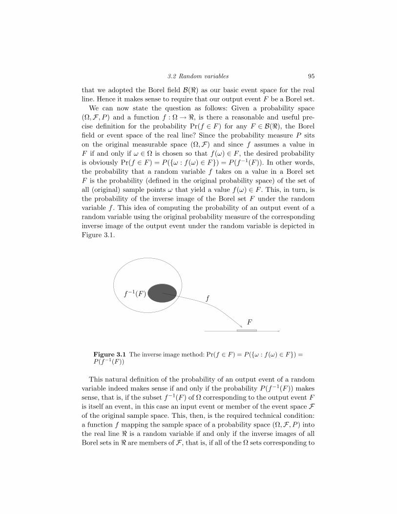
3.2 Random variables 95

that we adopted the Borel field B(ℜ) as our basic event space for the real

line. Hence it makes sense to require that our output event F be a Borel set.

We can now state the question as follows: Given a probability space

(Ω,F , P ) and a function f : Ω → ℜ, is there a reasonable and useful pre-

cise definition for the probability Pr(f ∈ F ) for any F ∈ B(ℜ), the Borel

field or event space of the real line? Since the probability measure P sits

on the original measurable space (Ω,F) and since f assumes a value in

F if and only if ω ∈ Ω is chosen so that f(ω) ∈ F , the desired probability

is obviously Pr(f ∈ F ) = P (ω : f(ω) ∈ F) = P (f−1(F )). In other words,

the probability that a random variable f takes on a value in a Borel set

F is the probability (defined in the original probability space) of the set of

all (original) sample points ω that yield a value f(ω) ∈ F . This, in turn, is

the probability of the inverse image of the Borel set F under the random

variable f . This idea of computing the probability of an output event of a

random variable using the original probability measure of the corresponding

inverse image of the output event under the random variable is depicted in

Figure 3.1.

f−1(F )f

F

Figure 3.1 The inverse image method: Pr(f ∈ F ) = P (ω : f(ω) ∈ F) =P (f−1(F ))

This natural definition of the probability of an output event of a random

variable indeed makes sense if and only if the probability P (f−1(F )) makes

sense, that is, if the subset f−1(F ) of Ω corresponding to the output event F

is itself an event, in this case an input event or member of the event space Fof the original sample space. This, then, is the required technical condition:

a function f mapping the sample space of a probability space (Ω,F , P ) into

the real line ℜ is a random variable if and only if the inverse images of all

Borel sets in ℜ are members of F , that is, if all of the Ω sets corresponding to

96 Random variables, vectors, and processes

output events (members of B(ℜ)) are input events (members of F). Unlike

some of the other pathological conditions that we have met, it is easy to

display some trivial examples where the technical condition is not met (as

we will see in Example [3.11]). We now formalize the definition.

Given a probability space (Ω,F , P ) a (real-valued) random variable is a

function f : Ω → ℜ with the property that if F ∈ B(ℜ), then also f−1(F ) =

ω : f(ω) ∈ F ∈ F .

Given a random variable f defined on a probability space (Ω,F , P ), the

set function

Pf (F )∆= P (f−1(F )) = P (ω : f(ω) ∈ F)= Pr(f ∈ F ); F ∈ B(ℜ) (3.19)

is well defined since by definition f−1(F ) ∈ F for all F ∈ B(ℜ). In the next

section the properties of distributions will be explored.

In some cases one may wish to consider a random variable with a more

limited range space than the real line, e.g., when the random variable is

binary. (Recall from Appendix A that the range space of f is the image of

Ω.) If so, ℜ can be replaced in the definition by the appropriate subset, say

A ⊂ ℜ. This is really just a question of semantics since the two definitions

are equivalent. One or the other view may, however, be simpler to deal with

for a particular problem.

A function meeting the condition in the definition we have given is said to

be measurable. This is because such functions inherit a probability measure

on their output events.

If a random variable has a distribution described by a pmf or a pdf with

a specific name, then the name is often applied also to the random variable;

e.g., a continuous random variable with a Gaussian pdf is called a Gaussian

random variable.

Examples

In every case we are given a probability space (Ω,F , P ). For the moment,

however, we will concentrate on the sample space Ω and the random variable

that is defined functionally on that space. Note that the function must be

defined for every value in the sample space if it is to be a valid function. On

the other hand, the function does not have to assume every possible value

in its range.

There is nothing particularly special about the names of the random vari-

ables. So far we have used the lower-case letter f . On occasion we will use

3.2 Random variables 97

other lower-case letters such as g and h. As we progress we will follow cus-

tom and more often use upper-case letters late in the alphabet, such as

X,Y,Z,U, V , and W . Capital Greek letters like Θ and Ψ are also popular.

The reader should keep the signal processing interpretation in mind while

considering these examples. Several very common types of signal processing

are considered, including quantization, sampling, and filtering.

[3.1] Let Ω = ℜ, the real line, and define the random variable X : Ω → Ω

by X(ω) = ω2 for all ω ∈ Ω. Thus the random variable is the square of

the sample point. Note that since the square of a real number is always

nonnegative, we could replace the range Ω by the range space [0,∞)

and consider X as a mapping X : Ω → [0,∞). Other random variables

mapping Ω into itself are Y (ω) = |ω|, Z(Ω) = sin(ω), U(ω) = 3 × ω +

321.5, and so on. We can also consider the identity mapping as a random

variable; that is, we can define a random variable W : Ω → Ω by W (ω) =

ω.

[3.2] Let Ω = ℜ as in Example [3.1] and define the random variable f :

ω → −V, V by

f(r) =

+V if r ≥ 0

−V otherwise.

This example is a variation of the binary quantizer of a real input consid-

ered in the introduction to Chapter 2. With this specific choice of output

levels it is also called a hard limiter.

So far we have used ω exclusively to denote the argument of the random

variable. We can, however, use any letter to denote the dummy variable (or

argument or independent variable) of the function, provided that we specify

its domain; that is, we do not need to use ω all the time to specify elements

of Ω: r, x, or any other dummy variable will do. We will, however, as a

convention, always use only lower-case letters to denote dummy variables.

When referring to a function, we will use several methods of specification.

Sometimes we will only give its name, say f ; sometimes we will specify its

domain and range, as in f : Ω → A; sometimes we will provide a specific

dummy variable, as in f(r); and sometimes we will provide the dummy

variable and its domain, as in f(r); r ∈ Ω. Finally, functions can be shown

with a place for the dummy variable marked by a period to avoid anointing

any particular dummy variable as being somehow special, as in f(·). These

various notations are really just different means of denoting the same thing

while emphasizing certain aspects of the functions. The only real danger

of this notation is the same as that of calculus and trigonometry: if one

98 Random variables, vectors, and processes

encounters a function, say sin t, does this mean the sine of a particular t

(and hence a real number) or does it mean the entire waveform of sin t for

all t? The distinction should be clear from the context, but the ambiguity

can be removed, for example, by defining something like sin t0 to mean a

particular value and sin t; t ∈ ℜ or sin(·) to mean the entire waveform.

[3.3] Let U be as in Example [3.1] and f as in Example [3.2]. Then the

function g : Ω → Ω defined by g(ω) = f(U(ω)) is also a random variable.

This relation is often abbreviated by dropping the explicit dependence

on ω to write g = f(U). More generally, any function of a function is

another function, called a “composite” function. Thus a function of a

random variable is another random variable. Similarly, one can consider

a random variable formed by a complicated combination of other random

variables – for example, g(ω) = (1/ω) sinh−1[π × ecos(|ω|3.4)].

[3.4] Let Ω = ℜk, k-dimensional Euclidean space. Occasionally it is of in-

terest to focus attention on the random variable which is defined as

a particular coordinate of a vector ω = (x0, x1, . . . , xk−1) ∈ ℜk. Toward

this end we can define for each i = 0, 1, . . . , k − 1 a sampling function (or

coordinate function) Πi : ℜk → ℜ as the following random variable:

Πi(ω) = Πi((x0, . . . , xk−1)) = xi.

The sampling functions are also called “projections” of the higher-

dimensional space onto the lower. (This is the reason for the choice of Π,

Greek P – not to be confused with the product symbol∏

– to denote the

functions.)

Similarly, we can define a sampling function for any product space, e.g.,

for sequence and waveform spaces.

⋆[3.5] Given a space A, an index set T , and the product space AT , define

as a random variable, for any fixed t ∈ T , the sampling function Πi :

AT → A as follows. Since any ω ∈ AT is a vector or function of the form

xs; s ∈ T , define for each t in T the mapping

Πt(ω) = Πt(xs; s ∈ T ) = xt.

Thus, for example, if Ω is a one-sided binary sequence space∏

i∈Z+

0, 1i = 0, 1Z+ ,

and hence every point has the form ω = (x0, x1, . . .), then

Π3((0, 1, 1, 0, 0, 0, 1, 0, 1, . . .)) = 0.

3.2 Random variables 99

As another example, if for all t in the index set ℜt is a replica of ℜ and Ω is

the space

ℜℜ =∏

t∈ℜℜt

of all real-valued waveforms x(t); t ∈ (−∞,∞), then for ω = sin t; t ∈ℜ, the value of the sampling function at the particular time t = 2π is

Π2π(sin t; t ∈ ℜ) = sin 2π = 0.

[3.6] Suppose that we have a one-sided binary sequence space 0, 1Z+ .

For any n ∈ 1, 2, . . ., define the random variable Yn by Yn(ω) =

Yn((x0, x1, x2, . . .)) = the index (time) of occurrence of the nth 1 in ω.

For example, Y2((0, 0, 0, 1, 0, 1, 1, 0, 1, . . .)) = 5 because the second sam-

ple to be 1 is x5.

[3.7] Say we have a one-sided sequence space Ω =∏

i∈Z+ℜi, where ℜi is

a replica of the real line for each i in the index set. Since every ω in this

space has the form x0, x1, . . . = xi; i ∈ Z+, we can define for each

positive integer n the random variable, depending on n,

Sn(ω) = Sn(xi; i ∈ Z+) = n−1n−1∑

i=0

xi

the arithmetic average or “mean” of the first n coordinates of the infinite

sequence.

For example, if ω = 1, 1, 1, 1, 1, 1, 1, . . ., then Sn = 1. This average is also

called a Cesaro mean or sample average or time average since the index

being summed over often corresponds to time; for example, we are adding the

outputs at times 0 through n − 1 in the preceding equation. Such arithmetic

means will later be seen to play a fundamental role in describing the long-

term average behavior of random processes. The arithmetic mean can also

be written using coordinate functions as

Sn(ω) = n−1n−1∑

i=0

Πi(ω), (3.20)

which we abbreviate to

Sn = n−1n−1∑

i=0

Πi (3.21)

by suppressing the dummy variable or argument ω. Equation (3.21) is short-

hand for (3.20) and says the same thing: the arithmetic average of the first

100 Random variables, vectors, and processes

n terms of a sequence is the sum of the first n coordinates or samples of the

sequence.

[3.8] As a generalization of the sample average consider weighted averages

of sequences. Such weighted averages occur in the convolutions of linear

system theory. Let Ω be the space∏

i∈Zℜi, where ℜi are all copies of

the real line. Suppose that hk; k = 0, 1, 2, . . . is a fixed sequence of real

numbers that can be used to form a weighted average of the coordinates

of ω ∈ Ω. Each ω in this space has the form ω = (. . . , x−1, x0, x1, . . .) =

xi; i ∈ Z and hence a weighted average can be defined for each integer

n:

Yn(ω) =

∞∑

k=0

hkxn−k.

Thus the random variable Yn is formed as a linear combination of the

coordinates of the sequence constituting the point ω in the double-sided

sequence space. This is a discrete time convolution of an input sequence

with a linear weighting. In linear system theory the weighting is called a

unit pulse response (or Kronecker delta response or δ-response), and it is the

discrete time equivalent of an impulse response. Note that we could also use

the sampling function notation to write Yn, as a weighted sum of the sample

random variables.

[3.9] In a similar fashion, complicated random variables can be defined on

waveform spaces. For example, let Ω =∏

t∈Rℜt, the space of all real-valued

functions of time such as voltage–time waveforms. For each T , define a

time average

YT (ω) = YT (x(t); t ∈ ℜ) = T−1

∫ T

0x(t) dt,

or given the impulse response h(t) of a causal, linear time-invariant sys-

tem, we define a weighted average

WT (ω) =

∫ ∞

0h(t)x(T − t) dt.

Are these also random variables? They are certainly functions defined on

the underlying sample space, but as one might suspect, the sample space of

all real-valued waveforms is quite large and contains some bizarre waveforms.

For example, the waveforms can be sufficiently pathological to preclude the

existence of the integrals cited (see Chapter 2 for a discussion of this point).

3.2 Random variables 101

These examples are sufficiently complicated to force us to look a bit closer at

a proper definition of a random variable and to develop a technical condition

that constrains the generality of our definition but ensures that the definition

will lead to a useful theory. It should be pointed out, however, that this

difficulty is no accident and is not easily solved: waveforms are truly more

complicated than sequences because of the wider range of possible waveforms

owing to the uncountability of the time variable. Continuous time random

processes are more difficult to deal with rigorously than are discrete time

processes. One can write equations such as the integrals and then find that

the integrals do not make sense even in the general Lebesgue sense. Often

fairly advanced mathematics are required to patch up the problems properly.

For purposes of simplicity we usually concentrate on sequences (and hence

on discrete time) rather than waveforms, and we gloss over the technical

problems when we consider continuous time examples. In Chapter 5 we will

return to add some rigor to the continuous case using the idea of mean

square convergence to define the integrals.

One must know the event space being considered in order to determine

whether or not a function is a random variable. Although we will virtually

always assume the usual event spaces (that is, the power set for discrete

spaces, the Borel field for the real line or subsets of the real line, and the

corresponding product event spaces for product sample spaces), it is useful

to consider some other examples to help clarify the basic definition.

[3.10] First consider (Ω,F , P ) where Ω is itself a discrete subset of the

real line ℜ, e.g., 0, 1 or Z+. If, as usual, we take F to be the power

set, then any function f : Ω → ℜ is a random variable. This follows since

the inverse image of any Borel set in ℜ must be a subset of Ω and hence

must be in the collection of all subsets of Ω.

Thus with the usual event space for a discrete sample space – the power set

– any function defined on the probability space is a random variable. This

is why all of the structure of event spaces and random variables is not seen

in elementary texts that consider only discrete spaces: there is no need.

It should be noted that for any Ω, discrete or not, if F is the power set,

then all functions defined on Ω are random variables. This fact is useful,

however, only for discrete sample spaces. The power set is not a useful event

space in the continuous case (as we cannot endow it with useful probability

measures).

If, however, F is not the power set, some functions defined on Ω are not

random variables, as the following simple example shows:

102 Random variables, vectors, and processes

[3.11] Let Ω be arbitrary, but let F be the trivial sigma-field Ω, ∅. On

this space it is easy to construct functions that are not random variables

(and hence are nonmeasurable functions). For example, let Ω = 0, 1and define f(ω) = ω, the identity function. Then f−1(0) = 0 is not

in F , and hence this simple function is not a random variable. In fact,

it is obvious that any function that assigns different values to 0 and 1 is

not a random variable. Note, however, that some functions are random

variables.

The problem illustrated by this example is that the input event space is not

big enough or “fine” enough to contain all input sets corresponding to output

events. This apparently trivial example suggests an important technique for

dealing with advanced random process theory, especially for continuous time

random processes: if the event space is not large enough to include the inverse

image of all Borel sets, then enlarge the event space to include all such events,

namely by using the power set as in Example [3.10]. Alternatively, we might

try to force F to contain all sets of the form f−1(F ), F ∈ B(ℜ); that is,

make F the sigma-field generated by such sets. Further treatment of this

subject is beyond the scope of the book. However, it is worth remembering

that if a sigma-field is not big enough to make a function a random variable,

it can often be enlarged to be big enough. This is not idle twiddling; such

a procedure is required for important applications, e.g., to make integrals

over time defined on a waveform space into random variables.

On a more hopeful tack, if the probability space (Ω,F , P ) is chosen with

Ω = ℜ and F = B(ℜ), then all functions f normally encountered in the

real world are in fact random variables. For example, continuous functions,

polynomials, step functions, trigonometric functions, limits of measurable

functions, maxima and minima of measurable functions, and so on are ran-

dom variables. It is, in fact, extremely difficult to construct functions on

Borel spaces that are not random variables. The same statement holds for

functions on sequence spaces. The difficulty is comparable to constructing

a set on the real line that is not a Borel set and is beyond the scope of this

book.

So far we have considered abstract philosophical aspects in the definition

of random variables. We are now ready to develop the probabilistic proper-

ties of the defined random variables.

3.3 Distributions of random variables 103

3.3 Distributions of random variables

3.3.1 Distributions

Suppose we have a probability space (Ω,F , P ) with a random variable, X,

defined on the space. The random variable X takes values on its range

space which is some subset A of ℜ (possibly A = ℜ). The range space A of

a random variable is often called the alphabet of the random variable. As we

have seen, since X is a random variable, we know that all subsets of Ω of

the form X−1(F ) = ω : X(ω) ∈ F, with F ∈ B(A), must be members of

F by definition. Thus the set function PX defined by

PX(F ) = P (X−1(F )) = P (ω : X(ω) ∈ F); F ∈ B(A) (3.22)

is well defined and assigns probabilities to output events involving the ran-

dom variable in terms of the original probability of input events in the orig-

inal experiment. The three written forms in Equation (3.22) are all read

as Pr(X ∈ F ) or “the probability that the random variable X takes on a

value in F .” Furthermore, since inverse images preserve all set-theoretic op-

erations (see Problem A.12), PX satisfies the axioms of probability as a

probability measure on (A,B(A)) – it is nonnegative, PX(A) = 1, and it is

countably additive. Thus PX is a probability measure on the measurable

space (A,B(A)). Therefore, given a probability space and a random variable

X, we have constructed a new probability space (A,B(A), PX ) where the

events describe outcomes of the random variable. The probability measure

PX is called the distribution of X (as opposed to a “cumulative distribution

function” of X to be introduced later).

If two random variables have the same distribution, then they are said

to be equivalent since they have the same probabilistic description, whether

or not they are defined on the same underlying space or have the same

functional form (see Problem 3.30).

A substantial part of the application of probability theory to practical

problems is devoted to determining the distributions of random variables,

that is, performing the “calculus of probability.” One begins with a probabil-

ity space. A random variable is defined on that space. The distribution of the

random variable is then derived, and this results in a new probability space.

This topic is called variously “derived distributions” or “transformations of

random variables” and is often developed in the literature as a sequence of

apparently unrelated subjects. When the points in the original sample space

can be interpreted as “signals,” then such problems can be viewed as “sig-

nal processing” and derived distribution problems are fundamental to the

analysis of statistical signal processing systems. We shall emphasize that all

104 Random variables, vectors, and processes

such examples are just applications of the basic inverse image formula (3.22)

and form a unified whole. In fact, this formula, with its vector analog, is one

of the most important applications of probability theory. Its specialization

to discrete input spaces using sums and to continuous input spaces using

integrals will be seen and used often throughout this book.

It is useful to bear in mind both the mathematical and the intuitive con-

cepts of a random variable when studying them. Mathematically, a random

variable, say X, is a “nice” (that is, measurable) real-valued function defined

on the sample space of a probability space (Ω,F , P ). Intuitively, a random

variable is something that takes on values at random. The randomness is

described by a distribution PX , that is, by a probability measure on an event

space of the real line. When doing computations involving random variables,

it is usually simpler to concentrate on the probability space (A,B(A), PX ),

where A is the range space of X, than on the original probability space

(Ω,F , P ). Many experiments can yield equivalent random variables, and the

space (A,B(A), PX ) can be considered as a canonical description of the ran-

dom variable that is often more useful for computation. The original space

is important, however, for two reasons. First, all distribution properties of

random variables are inherited from the original space. Therefore much of

the theory of random variables is just the theory of probability spaces spe-

cialized to the case of real sample spaces. If we understand probability spaces

in general, then we understand random variables in particular. Second, and

more important, we will often have many interrelated random variables de-

fined on a common probability space. Because of the interrelationships, we

cannot consider the random variables independently with separate probabil-

ity spaces and distributions. We must refer to the original space in order to

study the dependencies among the various random variables (or to consider

the random variables jointly as a random vector).

Since a distribution is a special case of a probability measure, in many

cases it can be induced or described by a probability function, i.e., a pmf or

a pdf. If a range space of the random variable is discrete or, more generally,

if there is a discrete subset of the range space A such that PX(A) = 1, then

there is a pmf, say pX , corresponding to the distribution PX . The two are

related via the formulas

pX(x) = PX(x), all x ∈ A, (3.23)

where A is the range space or alphabet of the random variable, and

PX(F ) =∑

x∈F

pX(x); F ∈ B(A). (3.24)

3.3 Distributions of random variables 105

In (3.23) both quantities are read as Pr(X = x).

The pmf and the distribution imply each other from (3.23) and (3.24),

and hence either formula specifies the random variable.

If the range space of the random variable is continuous and if a pdf fX

exists, then we can write the integral analog to (3.24):

PX(F ) =

∫

FfX(x) dx; F ∈ B(A). (3.25)

There is no direct analog of (3.23) for a pdf since a pdf is not a probability.

An approximate analog of (3.23) follows from the mean value theorem of

calculus. Suppose that F = [x, x + ∆x), where ∆x is extremely small. Then

if fX is sufficiently smooth, the mean value theorem implies that

PX([x, x + ∆x)) =

∫ x+∆x

xfX(α) dα ≈ fX(x)∆x, (3.26)

so that if we multiply a pdf fX(x) by a differential ∆x, it can be interpreted

as (approximately) the probability of being within ∆x of x. It is desirable,

however, to have an exact pair of results like (3.23) and (3.24) that show how

to go both ways, that is, to get the probability function from the distribution

as well as vice versa. From considerations of elementary calculus it seems

that we should somehow differentiate both sides of (3.25) to yield the pdf in

terms of the distribution. This is not immediately possible, however, because

F is a set and not a real variable. Instead to find a pdf from a distribution,

we use the intermediary of a cumulative distribution function or cdf. We

pause to give the formal definition.

Given a random variable X with distribution PX , the cumulative distri-

bution function or cdf FX is defined by

FX(α) = PX((−∞, α]) = PX(x : x ≤ α); α ∈ ℜ.

The cdf is seen to represent the cumulative probability of all values of the

random variable in the infinite interval from minus infinity up to and in-

cluding the real number argument of the cdf. The various forms can be

summarized as FX(α) = Pr(X ≤ α). If the random variable X is defined on

the probability space (Ω,F , P ), then by definition

FX(α) = P (X−1((−∞, α])) = P (ω : X(ω) ≤ α).If a distribution possesses a pdf, then the cdf and pdf are related through

the distribution and (3.25) by

FX(α) = P (X−1((−∞, α])) =

∫ α

−∞fX(x) dx; α ∈ ℜ. (3.27)

106 Random variables, vectors, and processes

The motivation for the definition of the cdf in terms of our previous dis-

cussion is now obvious. Since integration and differentiation are mutually

inverse operations, the pdf is determined from the cdf (and hence the dis-

tribution) by

fX(α) =dFX(α)

dα; α ∈ ℜ. (3.28)

where, as is customary, the right-hand side is shorthand for

dFX(x)

dx

∣∣∣∣x=α

,

the derivative evaluated at α. Alternatively, (3.28) also follows from the

fundamental theorem of calculus and the observation that

PX((a, b]) =

∫ b

afX(x) dx = FX(b) − FX(a). (3.29)

Thus (3.27) and (3.28) together show how to find a pdf from a distribution

and hence to provide the continuous analog of (3.23). Equation (3.23) is

useful, however only if the derivative, and hence the pdf, exists. Observe that

the cdf is always well defined (because the semi-infinite interval is a Borel

set and therefore an event), regardless of whether or not the pdf exists. This

is true in both the continuous and the discrete alphabet cases. For example,

if X is a discrete alphabet random variable with alphabet Z and pmf pX ,

then the cdf is

FX(x) =x∑

k=−∞pX(k), (3.30)

the analogous sum to the integral of (3.27). Furthermore, for this example,

the pmf can be determined from the cdf (as well as the distribution) as

pX(x) = FX(x) − FX(x − 1), (3.31)

a difference analogous to the derivative of (3.28).

It is desirable to use a single notation for the discrete and continuous

cases whenever possible. This is accomplished for expressing the distribution

in terms of the probability functions by using a Stieltjes integral, which is

3.3 Distributions of random variables 107

defined as

PX(F ) =

∫

FdFX (x) =

∫1F (x) dFX (x)

∆=

∑

x∈F

pX(x) if X is discrete

∫

FfX(x) dx if X has a pdf

. (3.32)

Thus (3.32) is a combination of both (3.24) and (3.25).

3.3.2 Mixture distributions

More generally, we may have a random variable that has both discrete and

continuous aspects and hence is not describable by either a pmf alone or

a pdf alone. For example, we might have a probability space (ℜ,B(ℜ), P ),

where P is described by a Gaussian pdf f(ω); ω ∈ ℜ. The sample point ω ∈ ℜis input to a soft limiter with output X(ω) – a device with input/output

characteristic X defined by

X(ω) =

−1 ω ≤ −1

ω ω ∈ (−1, 1)

1 1 ≤ ω

. (3.33)

As long as |ω| ≤ 1, X(ω) = ω. But for values outside this range, the output

is set equal to −1 or +1. Thus all of the probability density outside the

limiting range “piles up” on the ends so that Pr(X(ω) = 1) =∫ω≥1 f(ω)dω

is not zero. As a result X will have a mixture distribution, described by a

pdf in (−1, 1) and by a pmf at the points ±1.

Random variables of this type can be described by a distribution that is

the weighted sum of two other distributions – a discrete distribution and a

continuous distribution. The weighted sum is an example of a mixture dis-

tribution, that is, a mixture of probability measures as in Example [2.18].

Specifically, let P1 be a discrete distribution with corresponding pmf p, and

let P2 be a continuous distribution described by a pdf f . For any positive

weights c1, c2 with c1 + c2 = 1, the following mixture distribution PX is de-

fined for all F ∈ B(ℜ):

PX(F ) = c1P1(F ) + c2P2(F ) = c1

∑

k∈F

p(k) + c2

∫

Ff(x) dx

= c1

∑1F (k)p(k) + c2

∫1F (r)f(x) dx. (3.34)

108 Random variables, vectors, and processes

Continuing the example, the output of the limiter of (3.33) has a pmf and a

pdf. The pmf places probability 1/2 on ±1, while the pdf is Gaussian-shaped

for magnitudes less than unity (i.e., it is a truncated Gaussian pdf normalized

so that the pdf integrates to one over the range (−1, 1)). The constant c2 is

the integral of the input Gaussian pdf over (−1, 1) and c1 = 1 − c2. Observe

that the cdf for a random variable with a mixture distribution is

FX(α) = c1

∑

k:k≤α

p(k) + c2

∫ α

∞f(x) dx

= c1F1(α) + c2F2(α),

(3.35)

where F1 and F2 are the cdf’s corresponding to P1 and P2 respectively.

The combined notation for discrete and continuous alphabets using the

Stieltjes integral notation of (3.32) also can be used as follows. Given a

random variable with a mixture distribution of the form (3.34), then

PX(F ) =

∫

FdFX(x) =

∫1F (x) dFX (x); F ∈ B(ℜ). (3.36)

where∫

1F (x) dFX (x)∆= c1

∑1F (x)p(x) + c2

∫1F (x)f(x) dx. (3.37)

Observe that (3.36) and (3.37) include (3.32) as a special case where either c1

or c2 is 0. Equations (3.36) and (3.37) provide a general means for finding the

distribution of a random variable X given its cdf, provided the distribution

has the form of (3.35).

All random variables can be described by a cdf. But, more subtly, do

all random variables have a cdf of the form (3.35)? The answer is almost

yes. Certainly all of the random variables encountered in this book and

in engineering practice have this form. It can be shown, however, that the

most general cdf has the form of a mixture of three cdf’s: a continuous and

differentiable piece induced by a pdf, a discrete piece induced by a pmf,

and a third pathological piece. The third piece is an odd beast wherein the

cdf is something called a singular function – the cdf is continuous (it has no

jumps as it does in the discrete case), and is differentiable almost everywhere

(here “almost everywhere” means that the cdf is differentiable at all points

except some set F for which∫F dx = 0), but this derivative is 0 almost

everywhere and hence it cannot be integrated to find a probability! Thus for

this third piece, one cannot use pmf’s or pdf’s to compute probabilities. The

construction of such a cdf is beyond the scope of this text, but we can point

out for the curious that the typical example involves placing probability

3.3 Distributions of random variables 109

measures on the Cantor set that was considered in Problem 2.19. At any

rate, as such examples almost never arise in practice, we shall ignore them

and henceforth consider only random variables for which (3.36) and (3.37)

hold.

Although the general mixture distribution random variable has both dis-

crete and continuous pieces, for pedagogical purposes it is usually simplest

to treat the two pieces separately – i.e., to consider random variables that

have either a pdf or a pmf. Hence we will rarely consider mixture distribution

random variables and will almost always focus on those that are described

either by a pmf or by a pdf and not both.

To summarize our discussion, we will define a random variable to be a

discrete, continuous, or mixture random variable depending on whether it

is described probabilistically by a pmf, pdf, or mixture as in (3.36) and

(3.37) with c1, c2 > 0.

We note in passing that some texts endeavor to use a uniform approach

to mixture distributions by permitting pdf’s to possess Dirac delta or im-

pulse functions. The purpose of this approach is to permit the use of the

continuous ideas in discrete cases, as in our limiter output example. If the

cdf is differentiated, then a legitimate pdf results (without the need for a

pmf) if a delta function is allowed at the two discontinuities of the cdf. As

a general practice we prefer the Stieltjes notation, however, because of the

added notational clumsiness resulting from using pdf’s to handle inherently

discrete problems. For example, compare the notation for the geometric pmf

with the corresponding pdf that is written using Dirac delta functions.

3.3.3 Derived distributions

[3.12] Let (Ω,F , P ) be a discrete probability space with Ω a discrete sub-

set of the real line and F the power set. Let p be the pmf corresponding

to P , that is,

p(ω) = P (ω), all ω ∈ Ω.

(Note: there is a very subtle possibility for confusion here. One could

consider p(ω) to be a random variable because it satisfies the definition

for a random variable. We do not use it in this sense, however; we use

it as a pmf for evaluating probabilities in the context given. In addition,

no confusion should result because we rarely use lower-case letters for

random variables.) Let X be a random variable defined on this space.

Since the domain of X is discrete, its range space, A, is also discrete

(refer to the definition of a function to understand this point). Thus the

110 Random variables, vectors, and processes

probability measure PX must also correspond to a pmf, say pX ; that is,

(3.23) and (3.24) must hold. Then we can derive either the distribution

PX or the simpler pmf pX in order to complete a probabilistic description

of X. Using (3.22) yields

pX(x) = PX(x) = P (X−1(x)) =∑

ω:X(ω)=x

p(ω). (3.38)

Equation (3.38) provides a formula for computing the pmf and hence the

distribution of any random variable defined on a discrete probability space.

As a specific example, consider a discrete probability space (Ω,F , P ) with

Ω = Z+, F the power set of Ω, and P the probability measure induced by

the geometric pmf. Define a random variable Y on this space by

Y (ω) =

1 if ω even

0 if ω odd.

where we consider 0 (which has probability zero under the geometric pmf)

to be even. Thus we have a random variable Y : Z+ → 0, 1. Using the

formula (3.38) for the pmf for Y (ω) = 1 results in

pY (1) =∑

ω: ω even

(1 − p)k−1p =∑

k=2,4,...

(1 − p)k−1p

=p

(1 − p)

∞∑

k=1

((1 − p)2)k = p(1 − p)

∞∑

k=0

((1 − p)2)k

= p(1 − p)

1 − (1 − p)2=

1 − p

2 − p,

where we have used the standard geometric series summation formula (in a

thinly disguised variation of an example of Section 2.2.4). We can calculate

the remaining point in the pmf from the axioms of probability: pY (0) = 1 −pY (1). Thus we have found a nonobvious derived distribution by computing

a pmf via (3.38), a special case of (3.22). Of course, given the pmf, we could

now calculate the distribution from (3.24) for all four sets in the power set

of 0, 1.[3.13] Say we have a probability space (ℜ,B(ℜ), P ) where P is described

by a pdf g; that is, g is a nonnegative function of the real line with total

integral 1 and

P (F ) =

∫

r∈Fg(r) dr; F ∈ B(ℜ).

Suppose that we have a random variable X : ℜ → ℜ. We can use (3.22)

3.3 Distributions of random variables 111

or (3.25) to write a general formula for the distribution of X:

PX(F ) = P (X−1(F )) =

∫

r:X(r)∈Fg(r) dr.

Ideally, however, we would like to have a simpler description of X. In par-

ticular, if X is a “reasonable function” it should have either a discrete range

space (e.g., a quantizer) or a continuous range space (or possibly both, as

in the general mixture case). If the range space is discrete, then X can be

described by a pmf, and the preceding formula (with the requisite change of

dummy variable) becomes

pX(x) = PX(x) =

∫

r:X(r)=xg(r) dr.

If, however, the range space is continuous, then there should exist a pdf

for X, say fX , such that (3.25) holds. How do we find this pdf? As pre-

viously discussed, to find a pdf from a distribution, we first find the cdf

FX . Then we differentiate the cdf with respect to its argument to obtain

the pdf. As a nontrivial example, suppose that we have a probability space

(ℜ,B(ℜ), P ) with P the probability measure induced by the Gaussian pdf.

Define a random variable W : ℜ → ℜ by W (r) = r2; r ∈ ℜ. Following the

described procedure, we first attempt to find the cdf FW for W :

FW (w) = Pr(W ≤ w) = P (ω : W (ω) = ω2 ≤ w)= P ([−w1/2, w1/2]); if w ≥ 0.

The cdf is clearly 0 if w < 0. Since P is described by a pdf, say g (the specific

Gaussian form is not yet important), then

FW (w) =

∫ w1/2

−w1/2

g(r) dr.

If one should now try to plug in the specific form for the Gaussian density,

one would quickly discover that no closed form solution exists. Happily,

however, the integral does not have to be evaluated explicitly – we need

only its derivative. Therefore we can use the following handy formula from

elementary calculus for differentiating the integral:

d

dw

∫ b(w)

a(w)g(r) dr = g(b(w))

db(w)

dw− g(a(w))

da(w)

dw. (3.39)

112 Random variables, vectors, and processes

Application of the formula yields

fW (w) = g(w1/2)

(w−1/2

2

)

− g(−w1/2)

(

−w−1/2

2

)

. (3.40)

The final answer is found by plugging in the Gaussian form of g. For simplic-

ity we do this only for the special case where m = 0. Then g is symmetric;

that is, g(w) = g(−w), so that

fW (w) = w−1/2g(w1/2); w ∈ [0,∞),

and finally

fW (w) =w−1/2

√2πσ2

e−w/2σ2; w ∈ [0,∞).

This pdf is called a chi-squared pdf with one degree of freedom. Note that the

functional form of the pdf is valid only for the given domain. By implication

the pdf is zero outside the given domain – in this example, negative values

of W cannot occur. One should always specify the domain of the dummy

variable of a pdf; otherwise the description is incomplete.

In practice one is likely to encounter the following trick for deriving den-

sities for certain simple one-dimensional problems. The approach can be

used whenever the random variable is a monotonic (increasing or decreas-

ing) function of its argument. Suppose first that we have a random variable

Y = g(X), where g is a differentiable monotonically increasing function.

Since g is monotonic, it is invertible and we can write X = g−1(Y ), that

is, x = g−1(y) is the value of x for which g(x) = y. Then

FY (y) = Pr(g(X) ≤ y) = Pr(X ≤ g−1(y))

= FX(g−1(y)) =

∫ g−1(y)

−∞fX(x) dx.

From (3.39) the density can be found as

fY (y) =d

dyFY (y) = fX(g−1(y))

dg−1(y)

dy.

A similar result can be derived for a monotonically decreasing g except that a

minus sign results. The final formula is that if Y = g(X) and g is monotone,

then

fY (y) = fX(g−1(y))|dg−1(y)

dy|. (3.41)

This result is a one-dimensional special case of the so-called Jacobian

3.4 Random vectors and random processes 113

approach to derived distributions. The result could be used to solve the

previous problem by separately considering negative and nonnegative values

of the input r since r2 is a monotonic increasing function for nonnegative

r and monotonic decreasing for negative r. As in this example, the direct

approach from the inverse image formula is often simpler than using the

Jacobian “shortcut,” unless one is dealing with a monotonic function.

It can be seen that although the details may vary from application to ap-

plication, all derived distribution problems are solved by the general formula

(3.22). In some cases the solution will result in a pmf; in others the solution

will result in a pdf.

To review the general philosophy, one uses the inverse image formula

to compute the probability of an output event. This is accomplished by

finding the probability with respect to the original probability measure of

all input events that result in the given output event. In the discrete case

one concentrates on output events of the form X = x and thereby finds a

pmf. In the continuous case, one concentrates on output events of the form

X ≤ x and thereby finds a cdf. The pdf is then found by differentiating.

[3.14] As a final example of derived distributions, suppose that we are

given a probability space (Ω,B(Ω), P ) with Ω ⊂ ℜ. Define the identity

mapping X : Ω → Ω by X(ω) = ω. The identity mapping on the real line

with the Borel field is always a random variable because the measura-

bility requirement is automatically satisfied. Obviously the distribution

PX is identical to the original probability measure P . Thus all probabil-

ity spaces with real sample spaces provide examples of random variables

through the identity mapping. A random variable described in this form

instead of as a general function (not the identity mapping) on an under-

lying probability space is called a “directly given” random variable.

3.4 Random vectors and random processes

Thus far we have emphasized random variables, scalar functions on a sample

space that assume real values. In some cases we may wish to model processes

or measurements with complex values. Complex outputs can be considered

as two-dimensional real vectors with the components being the real and

imaginary parts or, equivalently, the magnitude and phase. This special case

can be equally well described as a single complex-valued random variable or

as a two-dimensional random vector.

More generally, we may have k-dimensional real vector outputs. A ran-

dom variable is a real-valued function on a sample space (with a technical

114 Random variables, vectors, and processes

condition), that is, a function mapping a sample space into the real line

ℜ. The obvious random vector definition is a vector-valued function defi-

nition. Under this definition, a random vector is a vector of random vari-

ables, a function mapping the sample space into ℜk instead of ℜ. Yet even

more generally, we may have vectors that are not finite-dimensional, e.g.,

sequences and waveforms whose values at each time are random variables.

This is essentially the definition of a random process. Fundamentally speak-

ing, both random vectors and random processes are simply collections of

random variables defined on a common probability space.

Given a probability space (Ω,F , P ), a finite collection of random variables

Xi; i = 0, 1, . . . , k − 1 is called a random vector. We will often denote a

random vector in boldface as X. Thus a random vector is a vector-valued

function X : Ω → ℜk defined by X = (X0,X1, . . . ,Xk−1) with each of the

components being a random variable. It is also common to use an ordinary

non-boldface X and let context indicate whether X has dimension 1 or not.

Another common notation for the k-dimensional random vector is Xk. Each

of these forms is convenient in different settings, but we begin with the

boldface notation in order to distinguish the random vectors from scalar

random variables. As we progress, however, the non-boldface notation will

be used with increasing frequency to match current style in the literature.

The boldface notation is still found, but it is far less common then it used to

be. When vectors are used in linear algebra manipulations with matrices and

other vectors, we will assume that they are column vectors so that strictly

speaking the vector should be denoted X = (X0,X1, . . . ,Xk−1)t, where t

denotes transpose.

A slightly different notation will ease the generalization to random pro-

cesses. A random vector X = (X0,X1, . . . ,Xk−1) can be defined as an in-

dexed family of random variables Xi; i ∈ T where T is the index set

Zk = 0, 1, . . . , k − 1. The index set in some examples will correspond to

time; e.g., Xi is a measurement on an experiment at time i for k differ-

ent times. We get a random process by using the same basic definition

with an infinite index set, which almost always corresponds to time. A ran-

dom process or stochastic process is an indexed family of random variables

Xi; t ∈ T or, equivalently, X(t); t ∈ T , defined on a common probabil-

ity space (Ω,F , P ). The process is said to be discrete time if T is discrete,

e.g., Z+ or Z, and continuous time if the index set is continuous, e.g., ℜor [0,∞). A discrete time random process is often called a time series. It is

said to be discrete alphabet or discrete amplitude if all finite-length random

vectors of random variables drawn from the random process are discrete

3.4 Random vectors and random processes 115

random vectors. The process is said to be continuous alphabet or continuous

amplitude if all finite-length random vectors of random variables drawn from

the random process are continuous random vectors. The process is said to

have a mixed alphabet if all finite-length random vectors of random variables

drawn from the random process are mixture random vectors.

Thus a random process is a collection of random variables indexed by

time, usually into the indefinite future and sometimes into the infinite past

as well. For each value of time t, Xt or X(t) is a random variable. Both

notations are used, but Xt or Xn is more common for discrete time processes

whereas X(t) is more common for continuous time processes. It is useful to

recall that random variables are functions on an underlying sample space

Ω and hence implicitly depend on ω ∈ Ω. Thus a random process (and a

random vector) is actually a function of two arguments, written explicitly as

X(t, ω); t ∈ T , ω ∈ Ω (or Xt(ω) – we use the first notation for the moment).

Observe that for a fixed value of time, X(t, ω) is a random variable whose

value depends probabilistically on ω. On the other hand, if we fix ω and

allow t to vary deterministically, we have either a sequence (T discrete) or a

waveform (T continuous). If we fix both t and ω, we have a number. Overall

we can consider a random process as a two-space mapping X : Ω × T → ℜor as a one-space mapping X : Ω → ℜT from sample space into a space of

sequences or waveforms.

There is a common notational ambiguity and hence confusion when deal-

ing with random processes. It is the same problem we encountered with

functions in the context of random variables at the beginning of the chap-

ter. The notation X(t) or Xt usually means a sample of the random process

at a specified time t, i.e., a random variable, just as sin t means the sine of a

specified value t. Often in the literature, however, the notation is used as an

abbreviation for X(t); t ∈ T or Xt; t ∈ T , that is, for the entire random

process or family of random variables. The abbreviation is the same as the

common use of sin t to mean sin t; t ∈ (−∞,∞), that is, the entire wave-

form and not just a single value. In summary, the common (and sometimes

unfortunate) ambiguity is in whether the dummy variable t means a specific

value or is implicitly allowed to vary over its entire domain. Of course, as

noted at the beginning of the chapter, the problem could be avoided by re-

serving a different notation to specify a fixed time value, say t0, but this is

usually not done, to avoid a proliferation of notation. In this book we will

attempt to avoid the potential confusion by using the abbreviations X(t)and Xt for the random processes when the index set is clear from context

and reserving the notation X(t) and Xt to mean the tth random variable of

116 Random variables, vectors, and processes

the process, that is, the sample of the random process at time t. The reader

should beware in reading other sources, however, because this sloppiness

will undoubtedly be encountered at some point in the literature; when this

happens one can only hope that the context will make the meaning clear.

There is also an ambiguity regarding the alphabet of the random process.

If X(t) takes values in At, then strictly speaking the alphabet of the random

process is∏

t∈T At, the space of all possible waveforms or sequences with

coordinate taking values in At. If all of the At are the same, say At = A, this

process alphabet is AT . In this case, however, the alphabet of the process is

commonly said to be simply A, the set of values from which all of the coor-

dinate random variables are drawn. We will frequently use this convention.

3.5 Distributions of random vectors

Since a random vector takes values in a space ℜk, one might expect that the

events in this space, that is, the members of the event space B(ℜ)k, should

inherit a probability measure from the original probability space. This is in

fact true as one would expect by analogy to scalar random variables. Also

analogous to the case of a random variable, the probability measure is called

a distribution and is defined as

PX(F )

= P (X−1(F )) = P (ω : X(ω) ∈ F)= P (ω : (X0(ω),X1(ω), . . . ,Xk−1(ω)) ∈ F), F ∈ B(ℜ)k, (3.42)

where the various forms are equivalent and all stand for Pr(X ∈ F ). Equa-

tion (3.42) is the vector generalization of the inverse image equation (3.22)

for random variables. Hence (3.42) is the fundamental formula for deriv-

ing vector distributions, that is, probability distributions describing random

vector events. Keep in mind that the random vectors might be composed of

a collection of samples from a random process.

By definition the distribution given by (3.22) is valid for each compo-

nent random variable. This does not immediately imply, however, that

the distribution given by (3.42) for events on all components together is

valid. As in the case of a random variable, the distribution will be valid if

the output events F ∈ B(ℜ)k have inverse images under X that are input

events, that is, if X−1(F ) ∈ F for every F ∈ B(ℜ)k. The following subsec-

tion treats this subtle issue in further detail, but the only crucial point for

our purposes is the following. Given that we consider real-valued vectors

X = (X0,X1, . . . ,Xk−1), knowing that each coordinate Xi is a random vari-

3.5 Distributions of random vectors 117

able (i.e., X−1i (F ) for each real event F ) guarantees that X−1(F ) ∈ F for

every F ∈ B(ℜ)k and hence the basic derived distribution formula is valid

for random vectors.

3.5.1 ⋆Multidimensional events

From the discussion following Example [2.11] we can at least resolve the

issue for certain types of output events, namely, events that are rectangles.

Rectangles are special events in that the values assumed by any component

in the event are not constrained by any of the other components (compare

a two-dimensional rectangle with a circle, as in Problem 2.36). Specifically

F ∈ B(ℜ)k is a rectangle if it has the form

F = x : si ∈ Fi; i = 0, 1, . . . , k − 1 =

k−1⋂

i=0

x : si ∈ Fi =

k−1∏

i=0

Fi,

where all Fi ∈ B(ℜ); i = 0, 1, . . . , k − 1 (refer to Figure 2.3(d) for a two-

dimensional illustration of such a rectangle). Because inverse images preserve

set operations (see Problem A.12), the inverse image of F can be specified

as the intersection of the inverse images of the individual events:

X−1(F ) = ω : Xi(ω) ∈ Fi; i = 0, 1, . . . , k − 1 =

k−1⋂

i=0

X−1i (Fi).

Since each of the Xi is a random variable, the inverse images of the individual

events X−1i (Fi) must all be in F . Since F is an event space, the intersection

of events must also be an event, and hence X−1(F ) is indeed an event.

Thus we conclude that the distribution is well defined for rectangles. As

to more general output events, we simply observe that a result from mea-

sure theory ensures that if (1) inverse images of rectangles are events and

(2) rectangles are used to generate the output event space, then the inverse

images of all output events are events. These two conditions are satisfied

by our definition. Thus the distribution of the random vector X is well de-

fined. Although a detailed proof of the measure theoretic result will not be

given, the essential concept can be given: any event in F can be approxi-

mated arbitrarily closely by finite unions of rectangles (e.g., a circle can be

approximated by lots of very small squares). The union of the rectangles is

an event. Finally, the limit of the events as the approximation gets better

must also be an event.

118 Random variables, vectors, and processes

3.5.2 Multidimensional probability functions

Given a probability space (Ω,F , P ) and a random vector X : Ω → ℜk, we

have seen that there is a probability measure PX that the random vector

inherits from the original probability space. With the new probability mea-

sure we define a new probability space (ℜk,B(ℜ)k, PX). As in the scalar case,

the distribution can be described by probability functions, that is, cdf’s and

either pmf’s or pdf’s (or both). If the random vector has a discrete range

space, then the distribution can be described by a multidimensional pmf

pX(x) = PX(x) = Pr(X = x) as

pX(F ) =∑

x∈F

pX(x) =∑

(x0,x1,...,xk−1)∈F

pX0,X1,...,Xk−1(x0, x1, . . . , xk−1),

where the last form points out the economy of the vector notation of the

previous line. If the random vector X has a continuous range space, then

in a similar fashion its distribution can be described by a multidimensional

pdf fX with PX(F ) =∫F fX(x) dx. In order to derive the pdf from the dis-

tribution, as in the scalar case, we use a cdf.

Given a k-dimensional random vector X, define its cumulative distribution

function FX by

FX(α) = FX0,X1,...,Xk−1(α0, α1, . . . , αk−1)

= PX(x : xi ≤ αi; i = 0, 1, . . . , k − 1).

In English, FX(x) = Pr(Xi ≤ xi; i = 0, 1, . . . , k − 1). Note that the cdf for

any value of its argument is the probability of a special kind of rectangle.

For example, if we have a two-dimensional random vector (X,Y ), then the

cdf FX,Y (α, β) = Pr(X ≤ α, Y ≤ β) is the probability of the semi-infinite

rectangle (x, y) : x ≤ α, y ≤ β.Observe that we can also write this probability in several other ways, e.g.,

FX(x) = PX

(k−1∏

i=0

(−∞, xi]

)

= P (ω : Xi(ω) ≤ xi; i = 0, 1, . . . , k − 1)

= P

(k−1⋂

i=0

X−1i ((−∞, xi])

)

.

Since integration and differentiation are inverses of each other, it follows

3.5 Distributions of random vectors 119

that

fX0,X1,...,Xk−1(x0, x1, . . . , xk−1)

=∂k

∂x0∂x1 . . . ∂xk−1FX0,X1,...,Xk−1

(x0, x1, . . . , xk−1).

As with random variables, random vectors can, in general, have discrete

and continuous parts with a corresponding mixture distribution. We will

concentrate on random vectors that are described completely by either pmf’s

or pdf’s. Also as with random variables, we can always unify notation using

a multidimensional Stieltjes integral to write

PX(F ) =

∫

FdFX(x) ; F ∈ B(ℜ)k,

where the integral is defined as the usual integral if X is described by a pdf,

as a sum if X is described by a pmf, and by a weighted average if X has both

a discrete and a continuous part. Random vectors are said to be continuous,

discrete, or mixture random vectors in accordance with the above analogy

to random variables.

3.5.3 Consistency of joint and marginal distributions

By definition a random vector X = (X0,X1, . . . ,Xk−1) is a collection of

random variables defined on a common probability space (Ω,F , P ). Alter-

natively, X can be considered to be a random vector that takes on values

randomly as described by a probability distribution PX, without explicit

reference to the underlying probability space. Either the original probability

measure P or the induced distribution PX can be used to compute probabil-

ities of events involving the random vector. In turn, PX may be induced by

a pmf pX or a pdf fX. From any of these probabilistic descriptions we can

find a probabilistic description for any of the component random variables

or any collection of thereof. That is, PX is evaluated on rectangles of the

form x = (x0, . . . , xk−1) : xi ∈ G for any G ∈ B(ℜ) as

PXi(G) = PX(x : xi ∈ G) , G ∈ B(ℜ). (3.43)

For example, given a value of i in 0, 1, . . . , k − 1, the distribution of the

random variable Xi is found by evaluating the distribution PX for the ran-

dom vector on one-dimensional rectangles where only the component Xi is

constrained to lie in some set – the rest of the components can take on any

value. Of course the probability can also be evaluated using the underlying

120 Random variables, vectors, and processes

probability measure P via the usual formula

PXi(G) = P (X−1i (G)).

Alternatively, we can consider this a derived distribution problem on

the vector probability space (ℜk,B(ℜ)k, PX) using a sampling function

Πi : ℜk → ℜ as in Example [3.4]. Specifically, let Πi(X) = Xi. Using (3.22)

we write

PΠi(G) = PX(Π−1i (G)) = PX(x : xi ∈ G). (3.44)

The two formulas (3.43) and (3.44) demonstrate that Πi and Xi are equiv-

alent random variables, and indeed they correspond to the same physical

events – the outputs of the ith coordinate of the random vector X. They

are related through the formula Πi(X(ω)) = Xi(ω). Intuitively, the two ran-

dom variables provide different models of the same thing. As usual, which

is “better” depends on which is the simpler model to handle for a given

problem.

Another fundamental observation implicit in these ruminations is that

there are many ways to compute the probability of a given event such as

“the ith coordinate of the random vector X takes on a value in an event F ,”

and all these methods must yield the same answer because they all can be

referred back to a common definition in terms of the underlying probability

measure P . This is called consistency; the various probability measures (P ,

PXi , and PX) are all consistent in that they assign the same number to any

given physical event for which they all are defined. In particular, if we have

a random process Xt; t ∈ T , then there is an infinite number of ways

we could form a random vector (Xt0 ,Xt1 , . . . ,Xtk−1) by choosing a finite

number k and sample times t0, t1, . . . , tk−1 and each of these would result

in a corresponding k-dimensional probability distribution PXt0 ,Xt1 ,...,Xtk−1.

The calculus derived from the axioms of probability implies that all of these

distributions must be consistent in the same sense, i.e., all must yield the

same answer when used to compute the probability of a given event.

The distribution PXi of a single component Xi of a random vector X

is referred to as a marginal distribution, while the distribution PX of the

random vector is called a joint distribution. As we have seen, joint and

marginal distributions are related by consistency with respect to the original

probability measure, i.e.,

PXi(G) = PX(x : xi ∈ G)= P (ω : Xi(ω) ∈ G)= Pr(Xi ∈ G). (3.45)

3.5 Distributions of random vectors 121

For the cases where the distributions are induced by pmf’s (marginal

pmf’s and joint pmf’s) or pdf’s (marginal pdf’s or joint pdf’s), the relation

becomes, respectively,

pXi(α)

=∑

x0,x1,...,xi−1,xi+1,...,xk−1

pX0,X1,...,Xk−1(x0, x1, . . . , xi−1, α, xi+1, . . . , xk−1)

or

fXi(α) =

∫

x0,...,xi−1,xi+1,...,xk−1

dx0 . . . dxi−1dxi+1 . . . dxk−1

fX0,...,Xk−1(x0, . . . , xi−1, α, xi+1, . . . , xk−1).

That is, we sum or integrate over all of the dummy variables corresponding to

the unwanted random variables in the vector to obtain the pmf or pdf for the

random variable Xi. The two formulas look identical except that one formula

sums for discrete random variables and the other integrates for continuous

ones. We repeat the fact that both formulas are simple consequences of

(3.45).

One can also use (3.43) to derive the cdf of Xi by setting G = (−∞, α].

The cdf is

FXi(α) = FX(∞,∞, . . . ,∞, α,∞, . . . ,∞),

where the α appears in the ith position. This equation states that Pr(Xi ≤α) = Pr(Xi ≤ α and Xj ≤ ∞), all j 6= i. The expressions for pmf’s and pdf’s

also can be derived from the expression for cdf’s.

The details of notation with k random variables can cloud the meaning

of the relations we are discussing. Therefore we rewrite them for the special

case of k = 2 to emphasize the essential form. Suppose that (X,Y ) is a

random vector. Then the marginal distribution of X is obtained from the

joint distribution of X and Y by leaving Y unconstrained, i.e., as in (3.43):

PX(F ) = PX,Y ((x, y) : x ∈ F); F ∈ B(ℜ).

Furthermore, the marginal cdf of X is

FX(α) = FX,Y (α,∞).

If the range space of the vector (X,Y ) is discrete, the marginal pmf of X is

pX(x) =∑

y

pX,Y (x, y).

122 Random variables, vectors, and processes

If the range space of the vector (X,Y ) is continuous and the cdf is differen-

tiable so that fX,Y (x, y) exists, the marginal pdf of X is

fX(x) =

∫ ∞

−∞fX,Y (x, y) dy,

with similar expressions for the distribution and probability functions for

the random variable Y .

In summary, given a probabilistic description of a random vector, we

can always determine a probabilistic description for any of the component

random variables of the random vector. This follows from the consistency

of probability distributions derived from a common underlying probabil-

ity space. It is important to keep in mind that the opposite statement is

not true. As considered in the introduction to this chapter, given all the

marginal distributions of the component random variables, we cannot find

the joint distribution of the random vector formed from the components

unless we further constrain the problem. This is true because the marginal

distributions provide none of the information about the interrelationships of

the components that is contained in the joint distribution.

In a similar manner we can deduce the distributions or probability func-

tions of “subvectors” of a random vector, that is, if we have the distribution

for X = (X0,X1, . . . ,Xk−1) and if k is big enough, we can find the distribu-

tion for the random vector (X1,X2) or the random vector (X5,X10,X15),

and so on. Writing the general formulas in detail in tedious and adds little

insight. The basic idea, however, is extremely important. One always starts

with a probability space (Ω,F , P ) from which one can proceed in many ways

to compute the probability of an event involving any combination of random

variables defined on the space. No matter how one proceeds, the probabil-

ity computed for a given event must be the same. In other words, all joint

and marginal probability distributions for random variables on a common

probability space must be consistent since they all follow from the common

underlying probability measure. For example, after finding the distribution

of a random vector X, the marginal distribution for the specific compo-

nent Xi can be found from the joint distribution. This marginal distribution

must agree with that obtained for Xi directly from the probability space.

As another possibility, one might first find a distribution for a subvector

containing Xi, say the vector Y = (Xi−1,Xi,Xi+1). This distribution can

be used to find the marginal distribution for Xi. All answers must be the

same since all can be expressed in the form P (X−1(F )) using the original

probability space must be consistent in the sense that they agree with one

another on events.

3.5 Distributions of random vectors 123

Examples

We now give examples of the computation of marginal probability func-

tions from joint probability functions.

[3.15] Say that we are given a pair of random variables X and Y such

that the random vector (X,Y ) has a pmf of the form

pX,Y (x, y) = r(x)q(y),

where r and q are both valid pmf’s. In other words, pX,Y is a product

pmf. Then it is easily seen that

pX(x) =∑

y

pX,Y (x, y) =∑

y

r(x)q(y)

= r(x)∑

y

q(y) = r(x).

Thus in the special case of a product distribution, knowing the marginal

pmf’s is enough to know the joint distribution.

[3.16] Consider flipping two fair coins connected by a piece of rubber

that is fairly flexible. Unlike the example where the coins were soldered

together, it is not certain that they will show the same face; it is, however,

more probable. To quantify the pmf, say that the probability of the pair

(0,0) is 0.4, the probability of the pair (1,1) is 0.4, and the probabilities

of the pairs (0,1) and (1,0) are each 0.1. As with the soldered-coins

case, this is clearly not a product distribution, but a simple computation

shows that as in Example [3.15], pX and pY both place probability 1/2

on 0, and 1. Thus this distribution, the soldered-coins distribution, and

the product distribution of Example [3.15] all yield the same marginal

pmf’s. The point again is that the marginal probability functions are not

enough to describe a vector experiment. We need the joint probability

function to describe the interrelations or dependencies among the random

variables.

[3.17] A gambler has a pair of very special dice: the sum of the two dice

comes up as seven on every roll. Each die has six faces with values in

A = 1, 2, 3, 4, 5, 6. All combinations have equal probability; e.g., the

probability of a one and a six has the same probability as a three and

a four. Although the two dice are identical, we will distinguish between

them by number for the purposes of assigning two random variables. The

outcome of the roll of the first die is denoted X and the outcome of the

roll of the second die is called Y so that (X,Y ) is a random vector taking

124 Random variables, vectors, and processes

values in A2, the space of all pairs of numbers drawn from A. The joint

pmf of X and Y is

pX,Y (x, y) =1

6, x + y = 7, (x, y) ∈ A2.

The pmf of X is determined by summing the pmf with respect to y.

However, for any given X ∈ A, the value of Y is determined: for example,

Y = 7 − X. Therefore the pmf of X is

pX(x) = 1/6, x ∈ A.

Note that this pmf is the same as one would derive for the roll of a single

unbiased die! Note also that the pmf for Y is identical with that for X.

Obviously, then, it is impossible to tell that the gambler is using unfair dice

as a pair from looking at outcomes of the rolls of each die alone. The joint

pmf cannot be deduced from the marginal pmf’s alone.

[3.18] Let (X,Y ) be a random vector with a pdf that is constant on the

unit disk in the XY plane; i.e.,

fX,Y (x, y) = C, x2 + y2 ≤ 1.

The constant C is determined by the requirement that the pdf integrate

to 1; i.e.,∫

x2+y2≤1C dxdy = 1.

Since this integral is just the area of a circle multiplied by C, we have

immediately that C = 1/π. For the moment, however, we leave the joint

pdf in terms of C and determine the pdf of X in terms of C by integrating

with respect to y:

fX(x) =

∫ +√

1−x2

−√

1−x2

C dy = 2C√

1 − x2 , x2 ≤ 1.

Observe that we could now also find C by a second integration:∫ +1

−12C√

1 − x2 dx = πC = 1,

or C = π−1. Thus the pdf of X is

fX(x) = 2π−1√

1 − x2 , x2 ≤ 1.

By symmetry Y has the same pdf. Note that the marginal pdf is not

constant, even though the joint pdf is. Furthermore, it is obvious that

3.6 Independent random variables 125

it would be impossible to determine the joint density from the marginal

pdf’s alone.

[3.19] Consider the two-dimensional Gaussian pdf of Example [2.17] with

k = 2, m = (0, 0)t, and Λ = λ(i, j) : λ(1, 1) = λ(2, 2) = 1, λ(1, 2) =

λ(2, 1) = ρ. Since the inverse matrix is

[1 ρ

ρ 1

]−1

=1

1 − ρ2

[1 −ρ

−ρ 1

],

the joint pdf for the random vector (X,Y ) is

fX,Y (x, y) =exp

(− 1

2(1−ρ2)(x2 + y2 − 2ρxy)

)

2π√

1 − ρ2, (x, y) ∈ ℜ2.

Here, ρ is called the “correlation coefficient”. between X and Y and

must satisfy ρ2 < 1 for Λ to be positive definite. To find the pdf of X we

complete the square in the exponent so that

fX,Y (x, y) =exp

(− (y−ρx)2

2(1−ρ2) − x2

2

)

2π√

1 − ρ2

=exp

(− (y−ρx)2

2(1−ρ2)

)

√2π(1 − ρ2)

exp(−x2

2

)

√2π

.

The pdf of X is determined by integrating with respect to y on (−∞,∞).

To perform this integration, refer to the form of the one-dimensional

Gaussian pdf with m = ρx (note that x is fixed while the integration

is with respect to y) and σ2 = 1 − ρ2. The first factor in the preceding

equation has this form. Because the one-dimensional pdf must integrate

to one, the pdf of X that results from integrating y out from the two-

dimensional pdf is also a one-dimensional Gaussian pdf; i.e.,

fX(x) = (2π)−1/2e−x2/2.

As in Examples [3.16], [3.17], and [3.18], Y has the same pdf as X. Note

that by varying ρ there is a whole family of joint Gaussian pdf’s with the

same marginal Gaussian pdf’s.

3.6 Independent random variables

In Chapter 2 it was seen that events are independent if the probability of a

joint event can be written as a product of probabilities of individual events.

126 Random variables, vectors, and processes

The notion of independent events provides a corresponding notion of inde-

pendent random variables and, as will be seen, results in random variables

being independent if their joint distributions are product distributions.

Two random variables X and Y defined on a probability space are inde-

pendent if the events X−1(F ) and Y −1(G) are independent for all F and

G in B(ℜ). A collection of random variables Xi, i = 0, 1, . . . , k − 1 is said

to be independent or mutually independent if all collections of events of

the form X−1i (Fi); i = 0, 1, . . . , k − 1 are mutually independent for any

Fi ∈ B(ℜ); i = 0, 1, . . . , k − 1.

Thus two random variables are independent if and only if their output

events correspond to independent input events. Translating this statement

into distributions yields the following.

Random variables X and Y are independent if and only if

PX,Y (F1 × F2) = PX(F1)PY (F2), all F1, F2 ∈ B(ℜ).

Recall that F1 × F2 is an alternative notation for∏2

i=1 Fi – we will fre-

quently use the alternative notation when the number of product events is

small. Note that a product and not an intersection is used here. The reader

should be certain that this is understood. The intersection is appropriate

if we refer back to the original ω events; that is, using the inverse image

formula to write this statement in terms of the underlying probability space

yields

P (X−1(F1) ∩ Y −1(F2) = P (X−1(F1))P (Y −1(F2)).

Random variables X0, . . . ,Xk−1 are independent or mutually independent

if and only if

PX0,...,Xk−1

(k−1∏

i=0

Fi

)=

k−1∏

i=0

PXi(Fi);

for all Fi ∈ B(ℜ); i = 0, 1, . . . , k − 1.

The general form for distributions can be specialized to pmf’s, pdf’s, and

cdf’s as follows. Two discrete random variables X and Y are independent if

and only if the joint pmf factors as

pX,Y (x, y) = pX(x)pY (y) ∀x, y.

A collection of discrete random variables Xi; i = 0, 1, . . . , k − 1 is mutually

3.6 Independent random variables 127

independent if and only if the joint pmf factors as

pX0,...,Xk−1(x0, . . . , xk−1) =

k−1∏

i=0

pXi(xi); ∀xi.

Similarly, if the random variables are continuous and described by pdf’s, then

two random variables are independent if and only if the joint pdf factors as

fX,Y (x, y) = fX(x)fY (y); ∀ x, y ∈ ℜ.

A collection of continuous random variables is independent if and only if the

joint pdf factors as

fX0,...,Xk−1(x0, . . . , xk−1) =

k−1∏

i=0

fXi(xi).

Two general random variables (discrete, continuous, or mixture) are in-

dependent if and only if the joint cdf factors as

FX,Y (x, y) = FX(x)FY (y) ; ∀ x, y ∈ ℜ.

A collection of general random variables is independent if and only if the

joint cdf factors as

FX0,...,Xk−1(x0, . . . , xk−1) =

k−1∏

i=0

FXi(xi); (x0, x1, . . . , xk−1) ∈ ℜk.

We have separately stated the two-dimensional case because of its sim-

plicity and common occurrence. The student should be able to prove the

equivalence of the general distribution form and the pmf form. If one does

not consider technical problems regarding the interchange of limits of inte-

gration, then the equivalence of the general form and the pdf form can also

be proved.

Independent identically distributed random vectors

A random vector is said to be independent, identically distributed or iid if

the coordinate random variables are independent and identically distributed;

that is, if

128 Random variables, vectors, and processes

• the distribution is a product distribution, i.e., it has the form

PX0,...,Xk−1

(k−1∏

i=0

Fi

)=

k−1∏

i=0

PXi(Fi)

for all choices of Fi ∈ B(ℜ), i = 0, 1, . . . , k − 1, and

• if all the marginal distributions are the same (the random variables are all equiv-

alent), i.e., if there is a distribution PX such that PXi(F ) = PX(F ); all F ∈ B(ℜ)

for all i.

For example, a random vector will have a product distribution if it has a

joint pdf or pmf that is a product pdf or pmf as described in Example [2.16].

The general property is easy to describe in terms of probability functions.

The random vector is iid if it has a joint pdf with the form

fX(x) =∏

i

fX(xi)

for some pdf fX defined on ℜ or if it has a joint pmf with the form

pX(x) =∏

i

pX(xi)

for some pmf pX defined on some discrete subset of the real line. Both of

these cases are included in the following statement: a random vector will be

iid if and only if its cdf has the form

FX(x) =∏

i

FX(xi)

for some cdf FX .

Note that, in contrast with earlier examples, the specification “product

distribution,” along with the marginal pdf’s or pmf’s or cdf’s, is sufficient

to specify the joint distribution.

3.7 Conditional distributions

The idea of conditional probability can be used to provide a general rep-

resentation of a joint distribution as a product, but a more complicated

product than arises with an iid vector. As one would hope, the complicated

form reduces to the simpler form when the vector is iid. The individual terms

of the product have useful interpretations.

The use of conditional probabilities allows us to break up many problems

in a convenient form and focus on the relations among random variables.

3.7 Conditional distributions 129

Examples to be treated include statistical detection, statistical classification,

and additive noise.

3.7.1 Discrete conditional distributions

We begin with the discrete alphabet case as elementary conditional proba-

bility suffices in this simple case. We can derive results that appear similar

for the continuous case, but nonelementary conditional probability will be

required to interpret the results correctly.

Begin with the simple case of a discrete random vector (X,Y ) with al-

phabet AX × AY described by a pmf pX,Y (x, y). Let pX and pY denote the

corresponding marginal pmf’s. Define for each x ∈ AX for which pX(x) > 0

the conditional pmf pY |X(y|x); y ∈ AY as the elementary conditional prob-

ability of Y = y given X = x, that is,

pY |X(y|x) = P (Y = y|X = x)

=P (Y = y and X = x)

P (X = x)

=P (ω : Y (ω) = y ∩ ω : X(ω) = x)

P (ω : X(ω) = x)

=pX,Y (x, y)

pX(x), (3.46)

where we have assumed that pX(x) > 0 for all suitable x to avoid dividing by

0. Thus a conditional pmf is just a special case of an elementary conditional

probability. For each x a conditional pmf is itself a pmf, since it is clearly

nonnegative and sums to 1:

∑

y∈AY

pY |X(y|x) =∑

y∈AY

pX,Y (x, y)

pX(x)=

1

pX(x)

∑

y∈AY

pX,Y (x, y)

=1

pX(x)pX(x) = 1.

We can compute conditional probabilities by summing conditional pmf’s,

i.e.,

P (Y ∈ F |X = x) =∑

y∈F

pY |X(y|x). (3.47)

The joint probability can be expressed as a product as

pX,Y (x, y) = pY |X(y|x)pX(x). (3.48)

130 Random variables, vectors, and processes

Unlike the independent case, the terms of the product do not each de-

pend on only a single independent variable. If X and Y are independent,

then pY |X(y|x) = pY (y) and the joint pmf reduces to the product of two

marginals.

Given the conditional pmf pY |X and the pmf pX , the conditional pmf with

the roles of the two random variables reversed can be computed by marginal

pmf’s by

pX|Y (x|y) =pX,Y (x, y)

pY (y)=

pY |X(y|x)pX(x)∑

u pY |X(y|u)pX(u), (3.49)

a result often referred to as Bayes’ rule.

The ideas of conditional pmf’s immediately extend to random vec-

tors. Suppose we have a random vector (X0,X1, . . . ,Xk−1) with a pmf

pX0,X1,...,Xk−1, then (provided none of the denominators are 0) we can define

for each l = 1, 2, . . . , k − 1 the conditional pmf’s

pXl|X0,...,Xl−1(xl|x0, . . . , xl−1) =

pX0,...,Xl(x0, . . . , xl)

pX0,...,Xl−1(x0, . . . , xl−1)

. (3.50)

Then simple algebra leads to the chain rule for pmf’s:

pX0,X1,...,Xn−1(x0, x1, . . . , xn−1)

=

(pX0,X1,...,Xn−1(x0, x1, . . . , xn−1)

pX0,X1,...,Xn−2(x0, x1, . . . , xn−2)

)pX0,X1,...,Xn−2(x0, x1, . . . , xn−2)

...

= pX0(x0)n−1∏

i=1

pX0,X1,...,Xi(x0, x1, . . . , xi)

pX0,X1,...,Xi−1(x0, x1, . . . , xi−1)

= pX0(x0)n−1∏

l=1

pXl|X0,...,Xl−1(xl|x0, . . . , xl−1), (3.51)

a product of conditional probabilities. This provides a general form of the

iid product form and reduces to the iid product form if indeed the random

variables are mutually independent. This formula plays an important role

in characterizing memory in random vectors and processes. It can be used

to construct joint pmf’s, and can be used to specify a random process.

3.7.2 Continuous conditional distributions

The situation with continuous random vectors is more complicated if rigor

is required, but the mechanics are similar. Again begin with the simple case

3.7 Conditional distributions 131

of two random variables X and Y with a joint distribution, now taken to be

described by a pdf fX,Y . We define the conditional pdf as an exact analog

to that for pmf’s:

fY |X(y|x)∆=

fX,Y (x, y)

fX(x). (3.52)

This looks the same as the pmf, but it is not the same because pmf’s are

probabilities and pdf’s are not. A conditional pmf is an elementary condi-

tional probability. A conditional pdf is not. It is also not the same as the

conditional pdf of Example [2.19] as in that case the conditioning event had

nonzero probability. The conditional pdf fY |X can, however, be related to a

probability in the same way that an ordinary pdf (and the conditional pdf

of Example [2.19]) can. An ordinary pdf is a density of probability, it is inte-

grated to compute a probability. In the same way, a conditional pdf can be

interpreted as a density of conditional probability, something you integrate

to get a conditional probability. Now, however, the conditioning event can

have probability zero and this does not really fit into the previous devel-

opment of elementary conditional probability. Note that a conditional pdf

is indeed a pdf, a nonnegative function that integrates to one. This follows

from∫

fY |X(y|x) dy =

∫fX,Y (x, y)

fX(x)dy

=1

fX(x)

∫fX,Y (x, y) dy

=1

fX(x)fX(x) = 1,

provided we require that fX(x) > 0 over the region of integration.

To be more specific, given a conditional pdf fY |X , we will make a tentative

definition of the (nonelementary) conditional probability that Y ∈ F given

X = x is

P (Y ∈ F |X = x) =

∫

FfY |X(y|x) dy. (3.53)

Note the close resemblance to the elementary conditional probability formula

in terms of conditional pmf’s of (3.47). For all practical purposes (and hence

for virtually all of this book), this constructive definition of nonelementary

conditional probability will suffice. Unfortunately it does not provide suffi-

cient rigor to lead to a useful advanced theory. Section 3.17 discusses the

problems and the correct general definition in some depth, but it is not

required for most applications.

132 Random variables, vectors, and processes

Via almost identical manipulations to the pmf case in (3.49), conditional

pdf’s satisfy a Bayes’ rule:

fX|Y (x|y) =fX,Y (x, y)

fY (y)=

fY |X(y|x)fX(x)∫fY |X(y|u)fX(u) du

. (3.54)

As a simple but informative example of a conditional pdf, consider the

generalization of Example [3.19] to the case of a two-dimensional vector

U = (X,Y ) with a Gaussian pdf having a mean vector (mX ,mY )t and a

covariance matrix

Λ =

[σ2

X ρσXσY

ρσXσY σ2Y

], (3.55)

where ρ is the correlation coefficient of X and Y . Straightforward algebra

yields

det(Λ) = σ2Xσ2

Y (1 − ρ2) (3.56)

Λ−1 =1

(1 − ρ2)

[1/σ2

X −ρ/(σXσY )

−ρ/(σXσY ) 1/σ2Y

](3.57)

so that the two-dimensional pdf becomes

fXY (x, y)

=1

2π√

detΛe−

12(x−mX ,y−mY )Λ−1(x−mX ,y−mY )t

=1

2πσXσY

√1 − ρ2

exp

(− 1

2(1 − ρ2)

×[(

x − mX

σX

)2

− 2ρ(x − mX)(y − mY )

σXσY+

(y − mY

σY

)2])

.(3.58)

A little algebra to rearrange the expression yields

fXY (x, y) =exp

(−1

2(x−mXσX

)2)

√2πσ2

X

exp

(−1

2

(y−mY −(ρσY /σX)(x−mX )√

1−ρ2σY

)2)

√2πσ2

Y (1 − ρ2)

(3.59)

from which it follows immediately that the conditional pdf is

fY |X(y|x) =

exp

(−1

2

(y−mY −(ρσY /σX)(x−mX )√

1−ρ2σY

)2)

√2πσ2

Y (1 − ρ2), (3.60)

3.8 Statistical detection and classification 133

which is itself a Gaussian density with variance σ2Y |X

∆= σ2

Y (1 − ρ2) and mean

mY |X∆= mY + ρ(σY /σX)(x − mX). Integrating y out of the joint pdf then

shows that as in Example [3.19] the marginal pdf is also Gaussian:

fX(x) =e−(x−mX)2/2σ2

X

√2πσ2

X

. (3.61)

A similar argument shows that fY (y) and fX|Y (x|y) are also Gaussian pdf’s.

Observe that if X and Y are jointly Gaussian, then they are also both

individually and conditionally Gaussian!

A chain rule for pdf’s follows in exactly the same way as that for pmf’s.

Assuming fX0,X1,...,Xi(x0, x1, . . . , xi) > 0,

fX0,X1,...,Xn−1(x0, x1, . . . , xn−1)

=fX0,X1,...,Xn−1(x0, x1, . . . , xn−1)

fX0,X1,...,Xn−2(x0, x1, . . . , xn−2)fX0,X1,...,Xn−2(x0, x1, . . . , xn−2)

...

= fX0(x0)

n−1∏

i=1

fX0,X1,...,Xi(x0, x1, . . . , xi)

fX0,X1,...,Xi−1(x0, x1, . . . , xi−1)

= fX0(x0)

k−1∏

l=1

fXl|X0,...,Xl−1(xl|x0, . . . , xl−1). (3.62)

3.8 Statistical detection and classification

Consider a simple, but nonetheless very important, example of the appli-

cation of conditional probability mass functions describing discrete random

vectors. Suppose that X is a binary random variable described by a pmf pX ,

with pX(1) = p. It might be one bit in some data coming through a modem.

You receive a random variable Y , which is equal to X with probability 1 − ǫ.

In terms of a conditional pmf this is

pY |X(y|x) =

ǫ x 6= y

1 − ǫ x = y. (3.63)

This can be written in a simple form using the idea of modulo 2 (or mod

2) arithmetic which will often be useful when dealing with binary variables.

Modulo 2 arithmetic or the “Galois field of 2 elements” arithmetic consists

134 Random variables, vectors, and processes

of an operation ⊕ called modulo 2 addition defined on the binary alphabet

0, 1 as follows:

0 ⊕ 1 = 1 ⊕ 0 = 1 (3.64)

0 ⊕ 0 = 1 ⊕ 1 = 0. (3.65)

The operation ⊕ corresponds to an “exclusive or” in logic; that is, it produces

a 1 if one or the other but not both of its arguments is 1. An equivalent

definition for the conditional pmf is

pY |X(y|x) = ǫx⊕y(1 − ǫ)1−x⊕y. (3.66)

For example, the channel over which the bit is being sent is noisy in that

the receiver occasionally makes an error. Suppose that it is known that the

probability of such an error is ǫ. The error might be very small on a good

phone line, but it might be very large if an evil hacker is trying to corrupt

your data. Given the observed Y , what is the best guess X(Y ) of what is

actually sent? In other words, what is the best decision rule or detection

rule for guessing the value of X given the observed value of Y ? A reasonable

parameter for judging the quality of an arbitrary rule X is the resulting

probability of error

Pe(X) = Pr(X(Y ) 6= X). (3.67)

A decision rule is optimal if it yields the smallest possible probability of error

over all possible decision rules. A little probability manipulation quickly

yields the optimal decision rule. Instead of minimizing the error probability,

we maximize the probability of being correct:

Pr(X = X) = 1 − Pe(X) =∑

(x,y):X(y)=x

pX,Y (x, y)

=∑

(x,y):X(y)=x

pX|Y (x|y)pY (y)

=∑

y

pY (y)

∑

x:X(y)=x

pX|Y (x|y)

=∑

y

pY (y)pX|Y (X(y)|y).

To maximize this sum, we want to maximize the terms within the sum

for each y. Clearly the maximum value of the conditional probability,

pX|Y (X(y)|y) = maxu pX|Y (u|y), will be achieved if we define the decision

3.8 Statistical detection and classification 135

rule X(y) to be the value of u achieving the maximum of pX|Y (u|y) over u,

that is, define X to be arg maxu pX|Y (u|y) (also denoted max−1u pX|Y (u|y)).

In words: the optimal estimate of X given the observation Y in the sense of

minimizing the probability of error is the most probable value of X given the

observation. This is called the maximum a posteriori or MAP decision rule.

In our binary example it reduces to choosing x = y if ǫ < 1/2 and x = 1 − y

if ǫ > 1/2. If ǫ = 1/2 you can give up and flip a coin or make an arbitrary

decision. (Why?) Thus the minimum (optimal) error probability over all

possible rules is min(ǫ, 1 − ǫ).

The astute reader will notice that having introduced conditional pmf’s

pY |X , the example considered the alternative pmf pX|Y . The two are easily

related by Bayes’ rule (3.49).

A generalization of the simple binary detection problem provides the typ-

ical form of a statistical classification system. Suppose that Nature selects a

“class” H, a random variable described by a pmf pH(h), which is no longer

assumed to be binary. Once the class is selected, Nature then generates a

random “observation” X according to a pmf pX|H . For example, the class

might be a medical condition and the observations the results of blood pres-

sure, patient’s age, medical history, and other information regarding the

patient’s health. Alternatively, the class might be an “input signal” put into

a noisy channel which has the observation X as an “output signal.” The

question is: given the observation X = x, what is the best guess H(x) of

the unseen class? If by “best” we adopt the criterion that the best guess is

the one that minimizes the error probability Pe = Pr(H(X) 6= H), then the

optimal classifier is again the MAP rule arg maxu pH|X(u|x). More generally

we might assign a cost Cy,h resulting if the true class is h and we guess y.

Typically it is assumed that Ch,h = 0, that is, the cost is zero if our guess is

correct. (In fact it can be shown that this assumption involves no real loss

of generality.) Given a classifier (classification rule, decision rule) h(x), the

Bayes risk is then defined as

B(h) =∑

x,h

Ch(x),hpH,X(h, x) , (3.68)

which reduces to the probability of error if the cost function is given by

Cy,h = 1 − δy,h. (3.69)

The optimal classifier in the sense of minimizing the Bayes risk is then

136 Random variables, vectors, and processes

found by observing that the inequality

B(h) =∑

x

pX(x)∑

h

Ch(x),hpH|X(h|x)

≥∑

x

pX(x)miny

(∑

h

Cy,hpH|X(h|x)

),

which lower bound is achieved by the classifier

h(x) = argminy

(∑

h

Cy,hpH|X(h|x)

)

, (3.70)

the minimum average Bayes risk classifier. This reduces to the MAP detec-

tion rule when Cy,h = 1 − δy,h.

3.9 Additive noise

The next examples of the use of conditional distributions treat the distri-

butions arising when one random variable (thought of as a “noise” term) is

added to another, independent random variable (thought of as a “signal”

term). This is an important example of a derived distribution problem that

yields an interesting conditional probability. The problem also suggests a

valuable new tool which will provide a simpler way of solving many similar

derived distributions – the characteristic function of random variables.

Discrete additive noise

Consider two independent random variables X and W and form a new

random variable Y = X + W . This could be a description of how errors are

actually caused in a noisy communication channel connecting a binary in-

formation source to a user. In order to apply the detection and classification

signal processing methods, we must first compute the appropriate condi-

tional probabilities of the output Y given the input X. To do this we begin

by computing the joint pmf of X and Y using the inverse image formula:

pX,Y (x, y) = Pr(X = x, Y = y) = Pr(X = x,X + W = y)

=∑

α,β:α=x,α+β=y

pX,W (α, β) = pX,W (x, y − x)

= pX(x)pW (y − x). (3.71)

Note that this formula only makes sense if y − x is one of the values in the

3.9 Additive noise 137

range space of W . Thus from the definition of conditional pmf’s,

pY |X(y|x) =pX,Y (x, y)

pX(x)= pW (y − x), (3.72)

an answer that should be intuitive: given the input is x, the output will equal

a certain value y if and only if the noise exactly makes up the difference,

i.e., W = y − x. Note that the marginal pmf for the output Y can be found

by summing the joint probability:

pY (y) =∑

x

pX,Y (x, y) =∑

x

pX(x)pW (y − x), (3.73)

a formula that is known as a discrete convolution or convolution sum.

Anyone familiar with convolutions knows that they can be unpleasant to

evaluate, so we postpone further consideration to the next section and turn

to the continuous analog.

The above development assumed ordinary arithmetic, but it is worth

pointing out that for discrete random variables sometimes other types of

arithmetic are appropriate, e.g., modulo 2 arithmetic for binary random

variables. The binary example of Section 3.8 can be considered as an addi-

tive noise example if we define a random variable W which is independent of

X and has a pmf pW (w) = ǫw(1 − ǫ)1−w; w = 0, 1 and where Y = X + W

is interpreted as modulo 2 arithmetic, that is, as Y = X ⊕ W . This additive

noise definition is easily seen to yield the conditional pmf of (3.63) and the

output pmf via a convolution. To be precise,

pX,Y (x, y) = Pr(X = x, Y = y) = Pr(X = x,X ⊕ W = y)

=∑

α,β:α=x,α⊕β=y

pX,W (α, β) = pX,W (x, y ⊕ x)

= pX(x)pW (y ⊕ x) (3.74)

and hence

pY |X(y|x) =pX,Y (x, y)

pX(x)= pW (y ⊕ x) (3.75)

and

pY (y) =∑

x

pX,Y (x, y) =∑

x

pX(x)pW (y ⊕ x), (3.76)

a modulo 2 convolution.

Continuous additive noise

138 Random variables, vectors, and processes

An entirely analogous formula arises in the continous case. Again suppose

that X is a random variable, a signal, with pdf fX , and that W is a ran-

dom variable, the noise, with pdf fW . The random variables X and W are

assumed to be independent. Form a new random variable Y , an observed

signal plus noise. The problem is to find the conditional pdf’s fY |X(y|x) and

fX|Y (x|y). The operation of producing an output Y from an input signal X

is called an additive noise channel in communications systems. The channel

is completely described by fY |X . The second pdf, fX|Y will prove useful later

when we try to estimate X given an observed value of Y .

Independence of X and W implies that the joint pdf is fX,W (x,w) =

fX(x)fW (w). To find the joint pdf fX,Y , first evaluate the joint cdf and

then take the appropriate derivative. The cdf is a straightforward derived

distribution calculation:

FX,Y (x, y) = Pr(X ≤ x, Y ≤ y)

= Pr(X ≤ x,X + W ≤ y)

=

∫ ∫

α,β:α≤x,α+β≤yfX,W (α, β) dα dβ

=

∫ x

−∞dα

∫ y−α

−∞dβfX(α)fW (β)

=

∫ x

−∞dαfX(α)FW (y − α).

Taking the derivatives yields

fX,Y (x, y) = fX(x)fW (y − x)

and hence

fY |X(y|x) = fW (y − x). (3.77)

The marginal pdf for the sum Y = X + W is then found as

fY (y) =

∫fX,Y (x, y) dx =

∫fX(x)fW (y − x) dx, (3.78)

a convolution integral of the pdf’s fX and fW , analogous to the convolution

sum found when adding independent discrete random variables. Thus the

evaluation of the pdf of the sum of two independent continuous random

variables is of the same form as the evaluation of the output of a linear

system with an input signal fX and an impulse response fW . We will later

see an easy way to accomplish this using transforms. The pdf fX|Y follows

3.9 Additive noise 139

from Bayes’ rule:

fX|Y (x|y) =fX(x)fW (y − x)∫fX(α)fW (y − α) dα

. (3.79)

It is instructive to work through the details of the previous example for

the special case of Gaussian random variables. For simplicity the means are

assumed to be zero and hence it is assumed that fX is N (0, σX), that fW

is N (0, σ2Y ), and that as in the example X and W are independent and

Y = X + W . From (3.77)

fY |X(y|x) = fW (y − x) =e−(y−x)2/2σ2

W

√2πσ2

W

(3.80)

from which the conditional pdf can be immediately recognized as being

Gaussian with mean x and variance σ2W , that is, as N (x, σ2

W ).

To evaluate the pdf fX|Y using Bayes’ rule, we begin with the denominator

fY of (3.54) and write

fY (y)

=

∫ ∞

−∞fY |X(y|α)fX(α) dα

=

∫ ∞

−∞

exp(− 1

2σ2W

(y − α)2)

√2πσ2

W

exp(− 1

2σ2X

α2)

√2πσ2

X

dα

=1

2πσXσW

∫ ∞

−∞exp

(−1

2

[y2 − 2αy + α2

σ2W

+α2

σ2X

])dα

=exp

(− y2

2σ2W

)

2πσXσW

∫ ∞

−∞exp

(−1

2

[α2(

1

σ2X

+1

σ2W

) − 2αy

σ2W

])dα. (3.81)

This convolution of two Gaussian “signals” can be accomplished using an old

trick called “complete the square.” Call the integral in the square brackets

at the end of the above equation I and note that integrand resembles

exp

(−1

2(α − m

σ)2)

.

We know from (B.13) in Appendix B that this integrates to∫ ∞

−∞exp

(−1

2(α − m

σ)2)

dα =√

2πσ2 (3.82)

since a Gaussian pdf integrates to 1. The trick is to modify I to resemble

140 Random variables, vectors, and processes

this integral with an additional factor. Compare the two exponents:

−1

2

[α2

(1

σ2X

+1

σ2W

)− 2αy

σ2W

]

with

−1

2

(α − m

σ

)2

= −1

2

[α2

σ2− 2

αm

σ2+

m2

σ2

].

The exponent from I will equal the left two terms of the expanded exponent

in the known integral if we choose

1

σ2=

1

σ2W

+1

σ2X

or, equivalently,

σ2 =σ2

Xσ2W

σ2X + σ2

W

, (3.83)

and if we choose

y

σ2W

=m

σ2

or, equivalently,

m =σ2

σ2W

y. (3.84)

Using (3.83)–(3.84) we have that

α2

(1

σ2X

+1

σ2W

)− 2αy

σ2W

=

(α − m

σ

)2

− m2

σ2,

where the addition of the leftmost term is “completing the square.” With

this identification and again using (3.83)–(3.84) we have that

I =

∫ ∞

−∞exp

(−1

2

[(α − m

σ2

)2

− m2

σ2

])dα

=√

2πσ2 exp

(m2

2σ2

), (3.85)

3.9 Additive noise 141

which implies that

fY (y) =exp

(−1

2y2

σ2W

)

2πσXσW

√2πσ2 exp

(m2

2σ2

)

=exp

(−1

2y2

σ2X

+σ2W

)

√2π(σ2

X + σ2W )

. (3.86)

In other words, fY is N (0, σ2X + σ2

W ) and we have shown that the sum of

two zero-mean independent Gaussian random variables is another zero-mean

Gaussian random variable with variance equal to the sum of the variances

of the two random variables being added.

Finally we turn to the a posteriori probability fX|Y . From Bayes’ rule and

a lot of algebra

fX|Y (x|y) = fY |X(y|x)fX(x)/fY (y)

=exp

(− 1

2σ2W

(y − x)2)

√2πσ2

W

exp(− 1

2σ2X

x2)

√2πσ2

X

/exp

(−1

2y2

σ2X

+σ2W

)

√2π(σ2

X + σ2W )

=exp

(−1

2

[y2−2yx+x2

σ2W

+ x2

σ2X

− y2

σ2X

+σ2W

])

√2πσ2

Xσ2W /(σ2

X + σ2W )

=exp

(− 1

2σ2Xσ2

W /(σ2X+σ2

W )(x − yσ2

X/(σ2X + σ2

W ))2)

√2πσ2

Xσ2W /(σ2

X + σ2W )

. (3.87)

In words: fX|Y (x|y) is a Gaussian pdf

N(

σ2X

σ2X + σ2

W

y,σ2

Xσ2W

σ2X + σ2

W

).

The mean of a conditional distribution is called a conditional mean and the

variance of a conditional distribution is called a conditional variance.

Continuous additive noise with discrete input

Additive noise provides a situation in which mixed distributions having

both discrete and continuous parts naturally arise. Suppose that the signal X

is binary, say with pmf pX(x) = px(1 − p)1−x. The noise term W is assumed

to be a continuous random variable described by pdf fW (w), independent of

X, with variance σ2W . The observation is defined by Y = X + W . In this case

142 Random variables, vectors, and processes

the joint distribution is not defined by a joint pmf or a joint pdf, but by a

combination of the two. Some thought may lead to the reasonable guess that

the continuous observation given the discrete signal should be describable

by a conditional pdf fY |X(y|x) = fW (y − x), where the conditional pdf is of

the elementary variety, the given event has nonzero probability. To prove

that this is in fact correct, consider the elementary conditional probability

Pr(Y ≤ y|X = x), for x = 0, 1. This is recognizable as the conditional cdf

for Y given X = x, so that the desired conditional density is given by

fY |X(y|x) =d

dyPr(Y ≤ y|X = x). (3.88)

The required probability is evaluated using the independence of X and W

as

Pr(Y ≤ y|X = x) = Pr(X + W ≤ y|X = x) = Pr(x + W ≤ y|X = x)

= Pr(W ≤ y − x) = FW (y − x).

Differentiating with respect to y gives

fY |X(y|x) = fW (y − x). (3.89)

The joint distribution is described in this case by a combination of a pmf

and a pdf. For example, to compute the joint probability that X ∈ F and

Y ∈ G is accomplished by

Pr(X ∈ F and Y ∈ G) =∑

F

pX(x)

∫

GfY |X(y|x) dy

=∑

F

pX(x)

∫

GfW (y − x) dy. (3.90)

Choosing F = ℜ yields the output distribution

Pr(Y ∈ G) =∑

pX(x)

∫

GfY |X(y|x) dy

=∑

pX(x)

∫

GfW (y − x) dy.

Choosing G = (−∞, y] provides a formula for the cdf FY (y), which can be

differentiated to yield the output pdf

fY (y) =∑

pX(x)fY |X(y|x) =∑

pX(x)fW (y − x), (3.91)

a mixed discrete convolution involving a pmf and a pdf (and exactly the

formula one expects in this mixed situation given the pure discrete and

continuous examples).

3.10 Binary detection in Gaussian noise 143

Continuing the parallel with the pure discrete and continuous cases, one

might expect that Bayes’ rule could be used to evaluate the conditional dis-

tribution in the opposite direction. Since X is discrete this is the conditional

pmf:

pX|Y (x|y) =fY |X(y|x)pX(x)

fY (y)=

fY |X(y|x)pX(x)∑

α pX(α)fY |X(y|α). (3.92)

Observe that unlike previously treated conditional pmf’s, this one is not

an elementary conditional probability since the conditioning event does not

have nonzero probability. Thus it cannot be defined in the original man-

ner, but must be justified in the same way as conditional pdf’s, that is, by

rewriting the joint distribution (3.90) as

Pr(X ∈ F and Y ∈ G) =

∫

GdyfY (y) Pr(X ∈ F |Y = y)

=

∫

GdyfY (y)

∑

F

pX|Y (x|y), (3.93)

so that pX|Y (x|y) does indeed play the role of a mass of conditional proba-

bility, that is,

Pr(X ∈ F |Y = y) =∑

F

pX|Y (x|y). (3.94)

Applying these results to the specific case of the binary input and Gaussian

noise, the conditional pmf of the binary input given the noisy observation is

pX|Y (x|y) =fW (y − x)pX(x)

fY (y)

=fW (y − x)pX(x)∑α pX(α)fW (y − α)

; y ∈ ℜ, x ∈ 0, 1. (3.95)

This formula now permits the analysis of a classical problem in communi-

cations, the detection of a binary signal in Gaussian noise.

3.10 Binary detection in Gaussian noise

The derivation of the MAP detector or classifier extends immediately to the

situation of a binary input random variable and independent Gaussian noise

just treated. As in the purely discrete case, the MAP detector X(y) of X

given Y = y is given by

X(y) = argmaxx

pX|Y (x|y) = argmaxx

fW (y − x)pX(x)∑α pX(α)fW (y − α)

. (3.96)

144 Random variables, vectors, and processes

Since the denominator of the conditional pmf does not depend on x (only

on y), given y the denominator has no effect on the maximization

X(y) = argmaxx

pX|Y (x|y) = argmaxx

fW (y − x)pX(x).

Assume for simplicity that X is equally likely to be 0 or 1 so that the rule

becomes

X(y) = argmaxx

pX|Y (x|y) = argmaxx

1√2πσ2

W

exp

(−1

2

(x − y)2

σ2W

).

The constant in front of the pdf does not affect the maximization. In ad-

dition, the exponential is a mononotically decreasing function of |x − y|, so

that the exponential is maximized by minimizing this magnitude difference,

i.e.,

X(y) = argmaxx

pX|Y (x|y) = argminx

|x − y|, (3.97)

which yields a final simple rule: see if x = 0 or 1 is closer to y as the best

guess of x. This choice yields the MAP detection and hence the minimum

probability of error. In our example this yields the rule

X(y) =

0 y < 0.5

1 y > 0.5. (3.98)

Because the optimal detector chooses the x that minimizes the Euclidean

distance |x − y| to the observation y, it is called a minimum distance detector

or rule. Because the guess can be computed by comparing the observation

to a threshold (the value midway between the two possible values of x), the

detector is also called a threshold detector .

Assumptions have been made to keep things fairly simple. The reader is

invited to work out what happens if the random variable X is biased and

if its alphabet is taken to be −1, 1 instead of 0, 1. It is instructive to

sketch the conditional pmf’s for these cases.

Having derived the optimal detector, it is reasonable to look at the re-

sulting, minimized, probability of error. This can be found using conditional

3.11 Statistical estimation 145

probability:

Pe = Pr(X(Y ) 6= X)

= Pr(X(Y ) 6= 0|X = 0)pX(0) + Pr(X(Y ) 6= 1|X = 1)pX(1)

= Pr(Y > 0.5|X = 0)pX(0) + Pr(Y < 0.5|X = 1)pX(1)

= Pr(W + X > 0.5|X = 0)pX(0) + Pr(W + X < 0.5|X = 1)pX(1)

= Pr(W > 0.5|X = 0)pX(0) + Pr(W + 1 < 0.5|X = 1)pX(1)

= Pr(W > 0.5)pX (0) + Pr(W < −0.5)pX(1)

where we have used the independence of W and X. These probabilities can

be stated in terms of the Φ-function of (2.78) as in (2.82), which combined

with the assumption that X is uniform and (2.84) yields

Pe =1

2

(1 − Φ

(0.5

σW

)+ Φ

(− 0.5

σW

))= Φ

(− 1

2σW

). (3.99)

3.11 Statistical estimation

Discrete conditional probabilities were seen to provide a method for guessing

an unknown class from an observation: if all incorrect choices have equal

costs so that the overall optimality criterion is to minimize the probability

of error, then the optimal classification rule is to guess that the class X =

k, where pX|Y (k|y) = maxz pX|Y (x|y), the maximum a-posteriori or MAP

decision rule. There is an analogous problem and solution in the continuous

case, but the result does not have as strong an interpretation as in the

discrete case. A more complete analogy will be derived in the next chapter.

As in the discrete case, suppose that a random variable Y is observed and

the goal is to make a good guess X(Y ) of another random variable X that is

jointly distributed with Y . Unfortunately in the continuous case it does not

make sense to measure the quality of such a guess by the probability of its

being correct because now that probability is usually zero. For example, if Y

is formed by adding a Gaussian signal X to an independent Gaussian noise

W to form an observation Y = X + W as in the previous section, then no

rule is going to recover X perfectly from Y . Nonetheless, intuitively there

should be reasonable ways to make such guesses in continuous situations.

Since X is continuous, such guesses are referred to as “estimation” or “pre-

diction” of X rather than as “classification” or “detection” as used in the

discrete case. In the statistical literature the general problem is referred to

as “regression”.

146 Random variables, vectors, and processes

One approach is to mimic the discrete approach on intuitive grounds. If

the best guess in the classification problem of a random variable X given an

observation Y is the MAP classifier XMAP(y) = argmaxxpX|Y (x|y), then a

natural analog in the continuous case is the so-called MAP estimator defined

by

XMAP(y) = argmaxxfX|Y (x|y), (3.100)

the value of x maximizing the conditional pdf given y. The advantage of

this estimator is that it is easy to describe and provides an immediate ap-

plication of conditional pdf’s paralleling that of classification for discrete

conditional probability. The disadvantage is that we cannot argue that this

estimate is “optimal” in the sense of optimizing some specified criterion,

it is essentially an ad hoc (but reasonable) rule. As an example of its use,

consider the Gaussian signal plus noise of the previous section. There it was

found that the pdf fX|Y (x|y) is Gaussian with mean yσ2X/(σ2

X + σ2W ). Since

the Gaussian density has its peak at its mean, in this case the MAP estimate

of X given Y = y is given by the conditional mean yσ2X/(σ2

X + σ2W ).

Knowledge of the conditional pdf is all that is needed to define another

estimator: the maximum likelihood or ML estimate of X given Y = y is

defined as the value of x that maximizes the conditional pdf fY |X(y|x),

the pdf with the roles of input and output reversed from that of the MAP

estimator. Thus

XML(y) = argmaxx

fY |X(y|x). (3.101)

Thus in the Gaussian case treated above, XML(Y ) = y.

The main interest in the ML estimator in some applications is that it

is sometimes simpler. It also does not require any assumption on the in-

put probabilities. The MAP estimator depends strongly on fX ; the ML

estimator does not depend on it at all. In the special case where the in-

put pdf fX is uniform and the conditional pdf fY |X(y|x) is 0 wherever

fX(x) = 0, then maximizing fY |X(y|x) over x is equivalent to maximizing

fX|Y (x|y) = fY |X(y|x)fX(x)/fY (y) over x so that the MAP estimator and

the ML estimator are the same.

3.12 Characteristic functions

We have seen that summing two random variables produces a new random

variable whose pmf or pdf is found by convolving the two pmf’s or pdf’s of

the original random variables. Anyone with an engineering background will

3.12 Characteristic functions 147

likely have had experience with convolution and know from experience that

convolutions can be somewhat messy to evaluate. To make matters worse,

if one wishes to sum additional independent random variables to the exist-

ing sum, say form YN =∑N

k=1 hN−kXk from an iid collection Xk, then

the result will be an N -fold convolution, a potential nightmare in all but the

simplest of cases. As in other engineering applications such as circuit design,

convolutions can be avoided by Fourier transform methods. In this subsec-

tion we describe the method as an alternative approach for the examples to

come. We begin with the discrete case.

Historically the transforms used in probability theory have been slightly

different from those in traditional Fourier analysis. For a discrete random

variable with pmf pX , define the characteristic function MX of the random

variable (or of the pmf) as

MX(ju) =∑

x

pX(x)ejux, (3.102)

where u is usually assumed to be real. Recalling the definition (2.34) of

the expectation of a function g defined on a sample space, choosing g(ω) =

ejuX(ω) shows that the characteristic function can be more simply defined

as

MX(ju) = E[ejuX ]. (3.103)

Thus characteristic functions, like probabilities, can be viewed as special

cases of expectations.

This transform, which is also referred to as an exponential transform or

operational transform, bears a strong resemblance to the discrete-parameter

Fourier transform

Fν(pX) =∑

x

pX(x)e−j2πνx (3.104)

and the z-transform

Zz(pX) =∑

x

pX(x)zx. (3.105)

In particular, MX(ju) = F−u/2π(pX) = Zeju(pX). As a result, all of the

properties of characteristic functions follow immediately from (are equiv-

alent to) similar properties from Fourier or z-transforms. As with Fourier

and z-transforms, the original pmf pX can be recovered from the transform

148 Random variables, vectors, and processes

MX by suitable inversion. For example, given a pmf pX(k); k ∈ ZN ,

1

2π

∫ π/2

−π/2MX(ju)e−iuk du =

1

2π

∫ π/2

−π/2

(∑

x

pX(x)ejux

)

e−iuk du

=∑

x

pX(x)1

2π

∫ π/2

−π/2eju(x−k) du

=∑

x

pX(x)δk−x = pX(k). (3.106)

Consider again the problem of summing two independent random vari-

ables X and W with pmf’s pX and pW and characteristic functions MX and

MW , respectively. If Y = X + W , as before we can evaluate the character-

istic function of Y as

MY (ju) =∑

y

pY (y)ejuy

where from the inverse image formula

pY (y) =∑

x,w:x+w=y

pX,W (x,w)

so that

MY (ju) =∑

y

(∑

x,w:x+w=y

pX,W (x,w)

)ejuy

=∑

y

(∑

x,w:x+w=y

pX,W (x,w)ejuy

)

=∑

y

(∑

x,w:x+w=y

pX,W (x,w)eju(x+w)

)

=∑

x,w

pX,W (x,w)eju(x+w)

where the last equality follows because the double sum for all y, x and w is

the sum for all x and w. This last sum factors, however, as

MY (ju) =∑

x,w

pX(x)pW (w)ejuxejuw

=∑

x

pX(x)ejux∑

w

pW (w)ejuw

= MX(ju)MW (ju), (3.107)

3.12 Characteristic functions 149

which shows that the transform of the pmf of the sum of independent random

variables is simply the product of the transforms.

Iterating (3.107) several times gives an extremely useful result that we

state formally as a theorem. It can be proved by repeating the above argu-

ment, but we shall later see a shorter proof.

Theorem 3.1 If Xi; i = 1, . . . , N are independent random variables with

characteristic functions MXi , then the characteristic function of the random

variable Y =∑N

i=1 Xi is

MY (ju) =N∏

i=1

MXi(ju). (3.108)

If the Xi are independent and identically distributed with common charac-

teristic function MX , then

MY (ju) = MNX (ju). (3.109)

As a simple example, the characteristic function of a binary random vari-

able X with parameter p = pX(1) = 1 − pX(0) is easily found to be

MX(ju) =

1∑

k=0

ejukpX(k) = (1 − p) + peju. (3.110)

If Xi; i = 1, . . . , n are independent Bernoulli random variables with iden-

tical distributions and Yn =∑n

k=1 Xi, then MYn(ju) = [(1 − p) + peju]n and

hence

MYn(ju) =

n∑

k=0

pYn(k)ejuk = ((1 − p) + peju)n

=

n∑

k=0

[(n

k

)(1 − p)n−kpk

]ejuk ,

where we have invoked the binomial theorem in the last step. For the equality

to hold, however, we have from the uniqueness of transforms that pYn(k)

must be the square bracketed term, that is, the binomial pmf

pYn(k) =

(n

k

)(1 − p)n−kpk; k ∈ Zn+1. (3.111)

As in the discrete case, convolutions can be avoided by transforming the

densities involved. The derivation is exactly analogous to the discrete case,

with integrals replacing sums in the usual way.

For a continous random variable X with pmf fX , define the characteristic

150 Random variables, vectors, and processes

function MX of the random variable (or of the pdf) as

MX(ju) =

∫fX(x)ejux dx. (3.112)

As in the discrete case, this can be considered as a special case of expectation

for continuous random variables as defined in (2.34) so that

MX(ju) = E[ejuX

]. (3.113)

The characteristic function is related to the the continuous-parameter

Fourier transform

Fν(fX) =

∫fX(x)e−j2πνx dx (3.114)

and the Laplace transform

Ls(fX) =

∫fX(x)e−sx dx (3.115)

by MX(ju) = F−u/2π(fX) = L−ju(fX).As a result, all of the properties of

characteristic functions of densities follow immediately from (are equivalent

to) similar properties from Fourier or Laplace transforms. For example, given

a well-behaved density fX(x); x ∈ ℜ with characteristic function MX(ju),

fX(x) =1

2π

∫ ∞

−∞MX(ju)e−jux du. (3.116)

Consider again the problem of summing two independent random vari-

ables X and Y with pdf’s fX and fW with characteristic functions MX and

MW , respectively. As in the discrete case it can be shown that

MY (ju) = MX(ju)MW (ju). (3.117)

Rather than mimic the proof of the discrete case, however, we postpone the

proof to a more general treatment of characteristic functions in Chapter 4.

As in the discrete case, iterating (3.117) several times yields the following

result, which now includes both discrete and continous cases.

Theorem 3.2 If Xi; i = 1, . . . , N are independent random variables with

characteristic functions MXi , then the characteristic function of the random

variable Y =∑N

i=1 Xi is

MY (ju) =N∏

i=1

MXi(ju). (3.118)

3.12 Characteristic functions 151

If the Xi are independent and identically distributed with common charac-

teristic function MX , then

MY (ju) = MNX (ju). (3.119)

As an example of characteristic functions and continuous random variables,

consider the Gaussian random variable. The evaluation requires a bit of

effort, either by using the “complete the square” technique of calculus or

by looking up in published tables. Assume that X is a Gaussian random

variable with mean m and variance σ2. Then

MX(ju) = E(ejuX) =

∫ ∞

−∞

1

(2πσ2)1/2e−(x−m)2/2σ2

ejux dx

=

∫ ∞

−∞

1

(2πσ2)1/2e−(x2−2mx−2σ2jux+m2)/2σ2

dx

=

∫ ∞

−∞

1

(2πσ2)1/2e−(x−(m+juσ2))2/2σ2

dx

ejum−u2σ2/2

= ejum−u2σ2/2. (3.120)

Thus the characteristic function of a Gaussian random variable with mean

m and variance σ2X is

MX(ju) = ejum−u2σ2/2. (3.121)

If Xi; i = 1, . . . , n are independent Gaussian random variables with

identical densities N (m,σ2) and Yn =∑n

k=1 Xi, then

MYn(ju) = [ejum−u2σ2/2]n = eju(nm)−u2(nσ2)/2, (3.122)

which is the characteristic function of a Gaussian random variable with mean

nm and variance nσ2.

The following maxim should be kept in mind whenever faced with sums

of independent random variables:

• When given a derived distribution problem involving the sum of independent

random variables, first find the characteristic function of the sum by taking the

product of the characteristic functions of the individual random variables. Then

find the corresponding probability function by inverting the transform. This tech-

nique is valid if the random variables are independent – they do not have to be

identically distributed.

152 Random variables, vectors, and processes

3.13 Gaussian random vectors

A random vector is said to be Gaussian if its density is Gaussian, that

is, if its distribution is described by the multidimensional pdf explained in

Chapter 2. The component random variables of a Gaussian random vector

are said to be jointly Gaussian random variables. Note that the symmetric

matrix Λ of the k-dimensional vector pdf has k(k + 1)/2 parameters and

that the vector m has k parameters. On the other hand, the k marginal

pdf’s together have only 2k parameters. Again we note the impossibility of

constructing joint pdf’s without more specification than the marginal pdf’s

alone. However, the marginals suffice to describe the entire vector if we also

know that the vector has independent components, e.g., the vector is iid. In

this case the matrix Λ is diagonal.

Although difficult to describe, Gaussian random vectors have several nice

properties. One of the most important of these properties is that linear or

affine operations on Gaussian random vectors produce Gaussian random

vectors. This result can be demonstrated with a modest amount of work

using multidimensional characteristic functions, the extension of transforms

from scalars to vectors.

The multidimensional characteristic function of a distribution is defined

as follows: Given a random vector X = (X0, . . . ,Xn−1) and a vector param-

eter u = (u0, . . . , un−1), the n-dimensional characteristic function MX(ju)

is defined by

MX(ju) = MX0,...,Xn−1(ju0, . . . , jun−1) = E[ejut

X

]

= E

[exp

(jn−1∑

k=0

ukXk

)]. (3.123)

It can be shown using multivariable calculus (problem 3.57) that a Gaussian

random vector with mean vector m and covariance matrix Λ has character-

istic function

MX(ju) = ejutm−u

tΛu/2

= exp

(j

n−1∑

k=0

ukmk − 1/2n−1∑

k=0

n−1∑

m=0

ukΛ(k,m)um

). (3.124)

Observe that the Gaussian characteristic function has the same form as

the Gaussian pdf – an exponential function of quadratic and linear terms.

However, unlike the pdf, the characteristic function depends on the covari-

ance matrix directly, whereas the pdf contains the inverse of the covariance

matrix. Thus the Gaussian characteristic function is in some sense simpler

3.14 Simple random processes 153

than the Gaussian pdf. As a further consequence of the direct dependence

on the covariance matrix, it is interesting to note that, unlike the Gaussian

pdf, the characteristic function is well defined even if Λ is only nonnegative

definite and not strictly positive definite. Previously we gave a definition of

a Gaussian random vector in terms of its pdf. Now we can give an alternate,

more general (in the sense that a strictly positive definite covariance matrix

is not required) definition of a Gaussian random vector and hence random

process):

• A random vector is Gaussian if and only if it has a characteristic function of the

form of (3.124).

This may seem strange at first thought – how can we define a vector to

be Gaussian by virtue of having a characteristic function of a certain form

while allowing that the pdf might not exist. If the pdf does not exist, then

of what is the characteristic function the transform? The answer is that in

general it is the transform of the distribution, which may exist even if the

pdf does not. We are effectively defining a Gaussian distribution here and

not a Gaussian pdf. We shall later see that if a distribution is Gaussian but

the pdf does not exist, then it is an example of what is called a singular

distribution and that if the covariance matrix is singular, it is not invertible.

3.14 Simple random processes

In this section several examples of random processes defined on simple prob-

ability spaces are given to illustrate the basic definition of an infinite col-

lection of random variables defined on a single space. In the next section

more complicated examples are considered by defining random variables on

a probability space which is the output space for another random process,

a setup that can be viewed as signal processing.

Examples

[3.22] Consider the binary probability space (Ω,F , P ) with Ω = 0, 1,Fthe usual event space, and P induced by the pmf p(0) = α and p(1) =

1 − α, where α is some constant, 0 ≤ α ≤ 1. Define a random process on

this space as follows:

X(t, ω) = cos(ωt) =

cos(t), t ∈ ℜ if ω = 1

1, t ∈ ℜ if ω = 0.

154 Random variables, vectors, and processes

Thus if a 1 occurs a cosine is sent forever, and if a 0 occurs a constant 1

is sent forever.

This process clearly has continuous time and at first glance it might appear

to have continuous amplitude also, but only two waveforms are possible,

a cosine and a constant. Thus the alphabet at each time contains at most

two values with nonzero probability and these possible values change with

time. Hence this process is in fact a discrete amplitude process and random

vectors drawn from this source are described by pmf’s. We can consider the

alphabet of the process to be either ℜT or [−1, 1]T , among other possibilities.

Fix time at t = π/2. Then X(π/2) is a random variable with pmf

pX(π/2)(x) =

α if x = 1

1 − α if x = 0.

The reader should try other instances of time. What happens at t =

0, 2π, 4π, 2mπ . . .?

[3.23] Consider a probability space (Ω,F , P ) with Ω = ℜ, F = B(ℜ), the

Borel field, and probability measure P induced by the pdf

f(r) =

1 if r ∈ [0, 1]

0 otherwise.

Again define the random process X(t) by X(t, ω) = cos(ωt); t ∈ ℜ.

Again the process is continuous time, but now it has mixed alphabet because

an uncountable infinity of waveforms is possible corresponding to all angular

frequencies between 0 and 1 so that X(t, ω) is a continuous random variable

except at t = 0, where X(0, ω) = 1 is a discrete random variable. If you

calculate the pdf of the random variable X(t) you see that it varies as a

function of time (Problem 3.33).

[3.24] Consider the probability space of Example [3.23], but cut it down

to the unit interval so that ([0, 1),B([0, 1)), P ) is the probability space,

where P is the probability measure induced by the pdf f(r) = 1; r ∈[0, 1). (So far this is just another model for the same thing.) For n =

1, 2 . . . ,Xn(ω) = bn(ω) = the nth digit binary expansion of ω, that is

ω =

∞∑

n=1

bn2−n

or equivalently ω = 0.b1b2b3 . . . in binary.

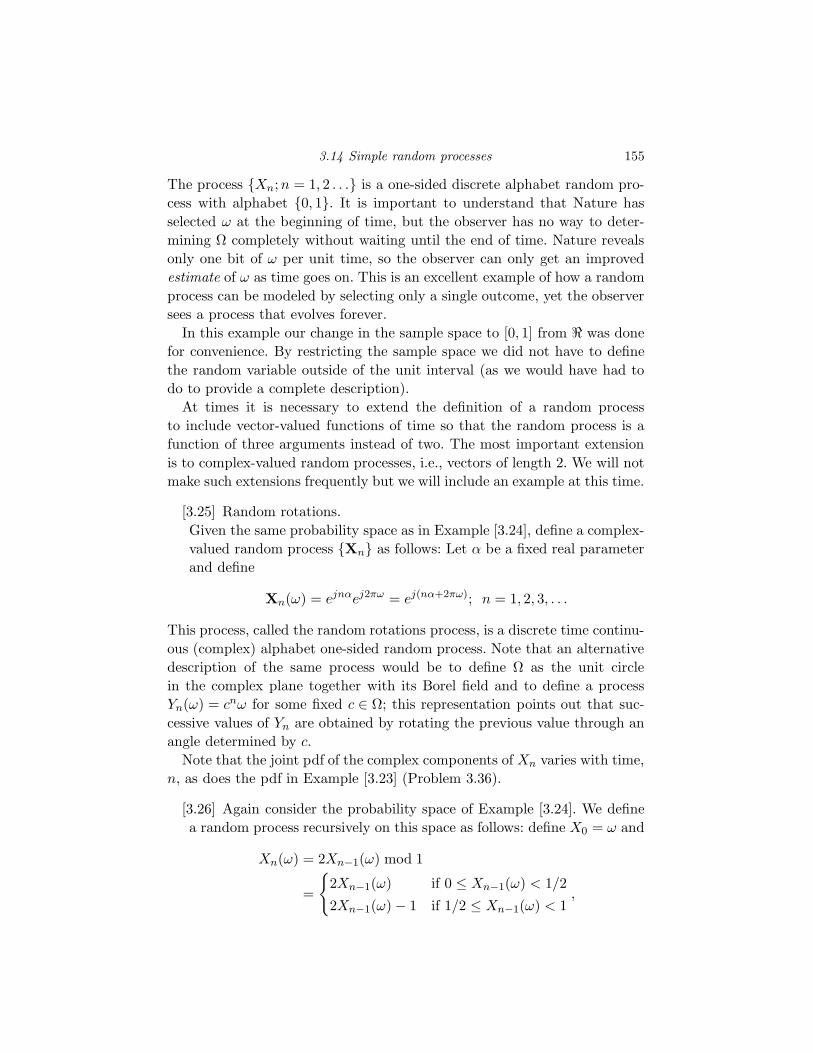
3.14 Simple random processes 155

The process Xn;n = 1, 2 . . . is a one-sided discrete alphabet random pro-

cess with alphabet 0, 1. It is important to understand that Nature has

selected ω at the beginning of time, but the observer has no way to deter-

mining Ω completely without waiting until the end of time. Nature reveals

only one bit of ω per unit time, so the observer can only get an improved

estimate of ω as time goes on. This is an excellent example of how a random

process can be modeled by selecting only a single outcome, yet the observer

sees a process that evolves forever.

In this example our change in the sample space to [0, 1] from ℜ was done

for convenience. By restricting the sample space we did not have to define

the random variable outside of the unit interval (as we would have had to

do to provide a complete description).

At times it is necessary to extend the definition of a random process

to include vector-valued functions of time so that the random process is a

function of three arguments instead of two. The most important extension

is to complex-valued random processes, i.e., vectors of length 2. We will not

make such extensions frequently but we will include an example at this time.

[3.25] Random rotations.

Given the same probability space as in Example [3.24], define a complex-

valued random process Xn as follows: Let α be a fixed real parameter

and define

Xn(ω) = ejnαej2πω = ej(nα+2πω); n = 1, 2, 3, . . .

This process, called the random rotations process, is a discrete time continu-

ous (complex) alphabet one-sided random process. Note that an alternative

description of the same process would be to define Ω as the unit circle

in the complex plane together with its Borel field and to define a process

Yn(ω) = cnω for some fixed c ∈ Ω; this representation points out that suc-

cessive values of Yn are obtained by rotating the previous value through an

angle determined by c.

Note that the joint pdf of the complex components of Xn varies with time,

n, as does the pdf in Example [3.23] (Problem 3.36).

[3.26] Again consider the probability space of Example [3.24]. We define

a random process recursively on this space as follows: define X0 = ω and

Xn(ω) = 2Xn−1(ω) mod 1

=

2Xn−1(ω) if 0 ≤ Xn−1(ω) < 1/2

2Xn−1(ω) − 1 if 1/2 ≤ Xn−1(ω) < 1,

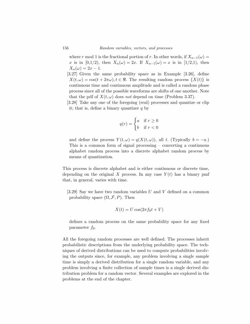
156 Random variables, vectors, and processes

where r mod 1 is the fractional portion of r. In other words, if Xn−1(ω) =

x is in [0,1/2), then Xn(ω) = 2x. If Xn−1(ω) = x is in [1/2,1), then

Xn(ω) = 2x − 1.

[3.27] Given the same probability space as in Example [3.26], define

X(t, ω) = cos(t + 2πω), t ∈ ℜ. The resulting random process X(t) is

continuous time and continuous amplitude and is called a random phase

process since all of the possible waveforms are shifts of one another. Note

that the pdf of X(t, ω) does not depend on time (Problem 3.37).

[3.28] Take any one of the foregoing (real) processes and quantize or clip

it; that is, define a binary quantizer q by

q(r) =

a if r ≥ 0

b if r < 0

and define the process Y (t, ω) = q(X(t, ω)), all t. (Typically b = −a.)

This is a common form of signal processing – converting a continuous

alphabet random process into a discrete alphabet random process by

means of quantization.

This process is discrete alphabet and is either continuous or discrete time,

depending on the original X process. In any case Y (t) has a binary pmf

that, in general, varies with time.

[3.29] Say we have two random variables U and V defined on a common

probability space (Ω,F , P ). Then

X(t) = U cos(2πf0t + V )

defines a random process on the same probability space for any fixed

parameter f0.

All the foregoing random processes are well defined. The processes inherit

probabilistic descriptions from the underlying probability space. The tech-

niques of derived distributions can be used to compute probabilities involv-

ing the outputs since, for example, any problem involving a single sample

time is simply a derived distribution for a single random variable, and any

problem involving a finite collection of sample times is a single derived dis-

tribution problem for a random vector. Several examples are explored in the

problems at the end of the chapter.

3.15 Directly given random processes 157

3.15 Directly given random processes

3.15.1 The Kolmogorov extension theorem

Consistency of distributions of random vectors of various dimensions plays a

far greater role in the theory and practice of random processes than simply

a means of checking the correctness of a computation. We have thus far ar-

gued that a necessary condition for a set of random vector distributions to

describe collections of samples taken from a random process is that the dis-

tributions be consistent , e.g., given marginals and joints we must be able to

compute the marginals from the joints. The Kolmogorov extension theorem

states that consistency is also sufficient for a family of finite-dimensional

vector distributions to describe a random process, that is, for there to exist

a well-defined random process that agrees with the given family of finite-

dimensional distributions. We state the theorem without proof as the proof

is far beyond the assumed mathematical prerequisites for this book. (The

interested reader is referred to [56, 7, 32].) Happily, however, it is often

straightforward, if somewhat tedious, to demonstrate that the conditions of

the theorem hold and hence that a proposed model is well-defined.

Theorem 3.3 Kolmogorov extension theorem

Suppose that one is given a consistent family of finite-dimensional distribu-

tions PXt0 ,Xt1 ,...,Xtk−1for all positive integers k and all possible sample times

ti ∈ T ; i = 0, 1, . . . , k − 1. Then there exists a random process Xt; t ∈ T that is consistent with this family. In other words, to describe a random

process completely, it is sufficient to describe a consistent family of finite-

dimensional distributions of its samples.

3.15.2 Independent identically distributed random processes

The next example extends the idea of an iid vector to provide one of the

most important random process models. Although such processes are sim-

ple in that they possess no memory among samples, they are a fundamental

building block for more complicated processes as well as being an important

example in their own right. In a sense these are the most random of all pos-

sible random processes because knowledge of the past does not help predict

future behavior.

A discrete time random process Xn is said to be independent identically

distributed or iid if all finite-dimensional random vectors formed by sampling

the process are iid; that is, if for any k and any collection of distinct sample

times t0, t1, . . . , tk−1, the random vector (Xt0 ,Xt1 , . . . ,Xtk−1) is iid.

158 Random variables, vectors, and processes

This definition is equivalent to the simpler definition of the introduction to

this chapter, but the more general form is adopted because it more closely

resembles definitions to be introduced later. Independent identically dis-

tributed random processes are often called Bernoulli processes, especially in

the binary case.

It can be shown with cumbersome but straightforward effort that the

random process of [3.24] is in fact iid. In fact, for any given marginal dis-

tribution there exists an iid process with that marginal distribution. Al-

though eminently believable, this fact requires the Kolmogorov extension

theorem, which states that a consistent family of finite-dimensional distri-

butions implies the existence of a random process described or specified

by those distributions. The demonstration of consistency for iid processes

is straightforward. Readers are encouraged to convince themselves for the

case of n-dimensional distributions reducing to (n − 1)-dimensional distri-

butions and, more specifically, of two-dimensional distributions implying

one-dimensional distributions

3.15.3 Gaussian random processes

A random process is Gaussian if the random vectors (Xt0 ,Xt1 , . . . ,Xtk−1)

are Gaussian. for all positive integers k and all possible sample times ti ∈T ; i = 0, 1, . . . , k − 1.

In order to describe a Gaussian process and verify the consistency

conditions of the Kolmogorov extension theorem, one has to provide

the covariance matrices Λ and mean vectors m for all random vectors

(Xt0 ,Xt1 , . . . ,Xtk−1) formed from a finite collection of ordered samples from

the process. This is accomplished by providing a mean function m(t); t ∈ Tand a covariance function Λ(t, s); t, s ∈ T , which then yield all of the re-

quired mean vectors and covariance matrices by sampling, that is, the mean

vector for (Xt0 ,Xt1 , . . . ,Xtk−1) is (m(t0),m(t1), . . . ,m(tk−1)) and the co-

variance matrix is Λ = Λ(tl, tj); l, j ∈ Zk.That this family of density functions are in fact consistent is much more

difficult to verify than was the case for iid processes, but it requires straight-

forward brute force in calculus rather than any deep mathematical ideas to

to do so.

The Gaussian random process in both discrete and continuous time is

virtually ubiquitous in the analysis of random systems. This is both because

the model is good for a wide variety of physical phenomena and because it

is extremely tractable for analysis.

3.16 Discrete time Markov processes 159

3.16 Discrete time Markov processes

An iid process is often referred to as a memoryless process because of the

independence among the samples. Such a process is both one of the simplest

random processes and one of the most random. It is simple because the joint

pmf’s are easily found as products of marginals. It is “most random” because

knowing the past (or future) outputs does not help improve the probabilities

describing the current output. It is natural to seek straightforward means

of describing more complicated processes with memory and to analyze the

properties of processes resulting from operations on iid processes. A general

approach towards modeling processes with memory is to filter memoryless

processes, i.e., to perform an operation (a form of signal processing) on

an input process which produces an output process that is not iid. In this

section we explore several examples of such a construction, all of which

provide examples of the use of conditional distributions for describing and

investigating random processes. All of the processes considered in this section

will prove to be examples of Markov processes, a class of random processes

possessing a specific form of dependence among current and past samples.

3.16.1 A binary Markov process

Suppose that Xn; n = 0, 1, . . . is a Bernoulli process with

pXn(x) =

p x = 1

1 − p x = 0, (3.125)

where p ∈ (0, 1) is a fixed parameter. Since the pmf does not depend on n,

the subscript is dropped and the pmf abbreviated to pX . The pmf can also

be written as

pX(x) = px(1 − p)1−x; x = 0, 1. (3.126)

Since the process is assumed to be iid,

pXn(xn) =n−1∏

i=0

pX(xi) = pw(xn)(1 − p)n−w(xn), (3.127)

where w(xn) is the number of nonzero xi in xn, called the Hamming weight

of the binary vector xn.

We consider using Xn as the input to a device which produces an output

binary process Yn. The device can be viewed as a signal processor or as a

linear filter. Since the process is binary, the most natural “linear” operations

are those in the binary alphabet using modulo 2 arithmetic as defined in

160 Random variables, vectors, and processes

(3.64)–(3.65). Consider the new random process Yn; n = 0, 1, 2, . . . defined

by

Yn =

Y0 n = 0

Xn ⊕ Yn−1 n = 1, 2, . . ., (3.128)

where Y0 is a binary equiprobable random variable (pY0(0) = pY0(1) = 0.5)

assumed to be independent of all of the Xn. This is an example of a linear

(modulo 2) recursion or difference equation. The process can also be defined

for n = 1, 2, . . . by

Yn =

1 if Xn 6= Yn−1

0 if Xn = Yn−1

.

This process is called a binary autoregressive process.

It should be apparent that Yn has quite different properties from Xn. In

particular, it depends strongly on past values. Since p < 1/2, Yn is more

likely to equal Yn−1 than it is to differ. If p is small, for example, Yn is likely

to have long runs of 0s and 1s. The sequence of random variables Yn is

defined on a common experiment, the outputs of the Xn process and an

independent selection of Y0. Thus Yn is itself a random process and all of

its joint pmf’s pY n(yn) = Pr(Y n = yn) should be derivable from the inverse

image formula. We proceed to solve this derived distribution and then to

interpret the result.

Using the inverse image formula in the general sense, which involves find-

ing a probability of an event involving Y n in terms of the probability of

an event involving Xn (and, in this case, the initial value Y0), yields the

following sequence of steps:

pY n(yn) = Pr(Y n = yn)

= Pr(Y0 = y0, Y1 = y1, Y2 = y2, . . . , Yn−1 = yn−1)

= Pr(Y0 = y0,X1 ⊕ Y0 = y1,X2 ⊕ Y1 = y2, . . . ,Xn−1 ⊕ Yn−2 = yn−1)

= Pr(Y0 = y0,X1 ⊕ y0 = y1,X2 ⊕ y1 = y2, . . . ,Xn−1 ⊕ yn−2 = yn−1)

= Pr(Y0 = y0,X1 = y1 ⊕ y0,X2 = y2 ⊕ y1, . . . ,Xn−1 = yn−1 ⊕ yn−2)

= pY0,X1,X2,X3,...,Xn−1(y0, y1 ⊕ y0, y2 ⊕ y1, . . . , yn−1 ⊕ yn−2)

= pY0(y0)

n−1∏

i=1

pX(yi ⊕ yi−1). (3.129)

The derivation used the facts that (1) a ⊕ b = c if and only if a = b ⊕ c, (2)

the independence of Y0, X1, X2, . . . , Xn−1, and (3) the fact that the Xn are

3.16 Discrete time Markov processes 161

iid. This formula completes the first goal, except possibly plugging in the

specific forms of pY0 and pX to get

pY n(yn) =1

2

n−1∏

i=1

pyi⊕yi−1(1 − p)1−yi⊕yi−1 . (3.130)

The marginal pmf’s for Yn can be evaluated by summing out the joints, e.g.,

pY1(y1) =∑

y0

pY0,Y1(y0, y1) =1

2

∑

y0

py1⊕y0(1 − p)1−y1⊕y0

=1

2; y1 = 0, 1.

In a similar fashion it can be shown that the marginals for Yn are all the

same:

pYn(y) =1

2; y = 0, 1; n = 0, 1, 2, . . . , (3.131)

and hence as with Xn the pmf can be abbreviated as pY , dropping the

subscript.

Observe in particular that unlike the iid Xn process,

pY n(yn) 6=n−1∏

i=0

pY (yi) (3.132)

(provided p 6= 1/2) and hence Yn is not an iid process and the joint pmf

cannot be written as a product of the marginals. Nonetheless, the joint pmf

can be written as a product of simple terms, as has been done in (3.130).

From the definition of conditional probability and (3.129)

pYl|Y0,Y1,...,Yl−1(yl|y0, y1, . . . , yl−1) =

pY l+1(yl+1)

pY l(yl)= pX(yl ⊕ yl−1) (3.133)

and (3.129) is then recognizable as the chain rule (3.51) for the joint pmf

pY n(yn).

Note that the conditional probability of the current output Yl given the

values for the entire past Yi; i = 0, 1, . . . , l − 1 depends only on the most

recent past output Yl−1! This property can be summarized nicely by also

deriving the conditional pmf

pYl|Yl−1(yl|yl−1) =

pYl−1,Yl(yl, yl−1)

pYl−1(yl−1)

, (3.134)

which with a little effort resembling the previous derivation can be evaluated

162 Random variables, vectors, and processes

as pyi⊕yi−1(1 − p)1−yi⊕yi−1. Thus the Yn process has the property that

pYi|Y0,Y1,...,Yi−1(yi|y0, y1, . . . , yi−1) = pYi|Yi−1

(yi|yi−1). (3.135)

A discrete time random process with this property is called a Markov pro-

cess or Markov chain. Such processes are among the most studied random

processes with memory.

3.16.2 The binomial counting process

We next turn to filtering a Bernoulli process that is linear in the ordinary

sense of real numbers. Now the input processes will be binary, but the output

process will have the nonnegative integers as an alphabet. Simply speaking,

the output process will be formed by counting the number of heads in a

sequence of coin flips.

Let Xn be iid binary random process with marginal pmf pX(1) = p =

1 − pX(0). Define a new one-sided random process Yn;n = 0, 1, . . . by

Yn =

Y0 = 0 n = 0∑n

k=1 Xk = Yn−1 + Xn n = 1, 2, . . .. (3.136)

For n ≥ 1 this process can be viewed as the output of a discrete time time-

invariant linear filter with Kronecker delta response hk given by hk = 1 for

k ≥ 0 and hk = 0 otherwise. From (3.136), each random variable Yn provides

a count of the number of 1s appearing in the Xn process through time n.

Because of this counting structure we have that either

Yn = Yn−1 or Yn = Yn−1 + 1; n = 2, 3, . . . (3.137)

In general, a discrete time process that satisfies (3.137) is called a counting

process since it is nondecreasing, and when it jumps, it is always with an

increment of 1. (A continuous alphabet counting process is similarly defined

as a process with a nondecreasing output which increases in time in steps

of 1.)

To completely describe this process it suffices to have a formula for the

joint pmf’s

pY1,...,Yn(y1, . . . , yn) = pY1(y1)

n∏

l=1

pYl|Y1,...,Yl−1(yl|y1, . . . , yl−1). (3.138)

When we have constructed one process Yn from an existing process Xn,we need not worry about consistency since we have defined the new process

on an underlying probability space (the output space of the original process),

3.16 Discrete time Markov processes 163

and hence the joint distributions must be consistent if they are correctly

computed from the underlying probability measure – the process distribution

for the iid process.

Since Yn is formed by summing n Bernoulli random variables, the pmf for

Yn follows immediately from (3.111); it is the binomial pmf and hence the

process is referred to as the binomial counting process.

The joint probabilities could be computed using the vector inverse image

formula as with the binary Markov source, but instead we focus on the

conditional distributions and compute them directly. The same approach

could have been used for the binary Markov example.

The conditional pmf’s are computed by describing probabilistically the

next output Yn of the process given the previous n − 1 outputs Y1, . . . , Yn−1.

For the binomial counting process, the next output is formed simply by

adding a binary random variable to the old sum. Thus all of the conditional

probability mass is concentrated on two values – the last value and the last

value plus 1. The conditional pmf’s can therefore be expressed as

pYn|Yn−1,...,Y1(yn|yn−1, . . . , y1)

= Pr(Yn = yn|Yl = yl; l = 1, . . . , yn−1)

= Pr(Xn = yn − yn−1|Yl = yl; l = 1, . . . , n − 1) (3.139)

= Pr(Xn = yn − yn−1|X1 = y1,Xi = yi − yi−1; i = 2, 3, . . . , n − 1),

since from the definition of the Yn process the conditioning event Yi =

yi; i = 1, 2, . . . , n − 1 is identical to the event X1 = y1,Xi = yi − yi−1; i =

2, 3, . . . , n − 1 and, given this event, the event Yn = yn is identical to the

event Xn = yn − yn−1. In words, the Yn will assume the given values if and

only if the Xn assume the corresponding differences since the Yn are defined

as the sum of the Xn. Now, however, the probability is entirely in terms of

the given Xi variables, in particular,

pYn|Yn−1,...,Y1(yn|yn−1, . . . , y1)

= pXn|Xn−1,...,X2,X1(yn − yn−1|yn−1 − yn−2, . . . , y2 − y1, y1). (3.140)

So far the development is valid for any process and has not used the fact

that the Xn are iid. If the Xn are iid, then the conditional pmf’s are

simply the marginal pmf’s since each Xn is independent of past Xk; k < n!

Thus we have that

pYn|Yn−1,...,Y1(yn|yn−1, . . . , y1) = pX(yn − yn−1). (3.141)

164 Random variables, vectors, and processes

and hence from the chain rule the vector pmf is (defining y0 = 0)

pY1,...,Yn(y1, . . . , yn) =

n∏

i=1

pX(yi − yi−1), (3.142)

providing the desired specification.

To apply this formula to the special case of the binomial counting process,

we need only plug in the binary pmf for pX to obtain the desired specification

of the binomial counting process:

pY1,...,Yn(y1, . . . , yn) =

n∏

i=1

p(yi−yi−1)(1 − p)1−(yi−yi−1),

where

yi − yi−1 = 0 or 1, i = 1, 2, . . . , n; y0 = 0. (3.143)

A similar derivation could be used to evaluate the conditional pmf for Yn

given only its immediate predecessor as:

pYn|Yn−1(yn|yn−1) = Pr(Yn = yn|Yn−1 = yn−1)

= Pr(Xn = yn − yn−1|Yn−1 = yn−1).

The conditioning event, however, depends only on values of Xk for k < n,

and Xn is independent of its past; hence

pYn|Yn−1(yn|yn−1) = pX(yn − yn−1). (3.144)

The same conclusion can be reached by the longer route of using the joint

pmf for Y1, . . . , Yn previously computed to find the joint pmf for Yn and

Yn−1, which in turn can be used to find the conditional pmf. Comparison

with (3.141) reveals that processes formed by summing iid processes (such

as the binomial counting process) have the property that

pYn|Yn−1,...,Y1(yn|yn−1, . . . , y1) = pYn|Yn−1

(yn|yn−1) (3.145)

or, equivalently,

Pr(Yn = yn|Yi = yi ; i = 1, . . . , n − 1) = Pr(Yn = yn|Yn−1 = yn−1),

(3.146)

that is, they are Markov processes. Roughly speaking, given the most recent

past sample (or the current sample), the remainder of the past does not

affect the probability of what happens next. Alternatively stated, given the

present, the future is independent of the past.

3.16 Discrete time Markov processes 165

3.16.3 ⋆Discrete random walk

As a second example of the preceding development, consider the random

walk defined as in (3.136), i.e., by

Yn =

0 n = 0∑n

k=1 Xk n = 1, 2, . . ., (3.147)

where the iid process used has alphabet 1,−1 and Pr(Xn = −1) = p. This

is another example of an autoregressive process since it can be written in

the form of a regression

Yn = Yn−1 + Xn, n = 1, 2, . . . (3.148)

One can think of Yn as modeling a drunk on a path who flips a coin at each

minute to decide whether to take one step forward or one step backward. In

this case the transform of the iid random variables is

MX(ju) = (1 − p)eju + pe−ju,

and hence using the binomial theorem of algebra we have that

MYn(ju) = ((1 − p)eju + pe−ju)n

=

n∑

k=0

[(n

k

)(1 − p)n−kpk

]eju(n−2k)

=∑

k=−n,−n+2,...,n−2,n

[(n

(n − k)/2

)(1 − p)(n+k)/2p(n−k)/2

]ejuk.

Comparison of this formula with the definition of the characteristic func-

tion reveals that the pmf for Yn is given by

pYn(k) =

(n

(n − k)/2

)(1 − p)(n+k)/2p(n−k)/2 ,

k = −n,−n + 2, . . . , n − 2, n.

Note that Yn must be even or odd depending on whether n is even or odd.

This follows from the nature of the increments.

3.16.4 The discrete time Wiener process

Again consider a process formed by summing an iid process as in (3.136).

This time, however, let Xn be an iid process with zero-mean Gaussian

marginal pdf’s and variance σ2. Then the process Yn defined by (3.136)

166 Random variables, vectors, and processes

is called the discrete time Wiener process. The discrete time, continuous

alphabet case of summing iid random variables is handled in virtually the

same manner as the discrete time, discrete alphabet case, with conditional

pdf’s replacing conditional pmf’s.

The marginal pdf for Yn is given immediately by (3.122) as N(0, nσ2X).

To find the joint pdf’s we evaluate the pdf chain rule of (3.62):

fY1,...,Yn(y1, . . . , yn) =

n∏

l=1

fYl|Y1,...,Yl−1(yl|y1, . . . , yl−1). (3.149)

To find the conditional pdf fYn|Y1,...,Yn−1(yn|y1, . . . , yn−1) we compute the

conditional cdf P (Yn ≤ yn|Yn−i = yn−i; i = 1, 2, . . . , n − 1). Analogous to

the discrete case, from the representation of (3.136) and the fact that the

Xn are iid we have that

P (Yn ≤ yn|Yn−i = yn−i; i = 1, 2, . . . , n − 1)

= P (Xn ≤ yn − yn−1|Yn−i = yn−i; i = 1, 2, . . . , n − 1)

= P (Xn ≤ yn − yn−1) = FX(yn − yn−1), (3.150)

and hence differentiating the conditional cdf to obtain the conditional pdf

yields

fYn|Y1,...,Yn−1(yn|y1, . . . , yn−1) =

∂

∂ynFX(yn − yn−1) = fX(yn − yn−1),

(3.151)

the continuous analog of (3.141). Application of the pdf chain rule then

yields the continuous analog to (3.142):

fY1,...,Yn(y1, . . . , yn) =n∏

i=1

fX(yi − yi−1). (3.152)

Finally suppose that fX is Gaussian with zero mean and variance σ2. Then

this becomes

fY n(yn) =exp

(− y2

12σ2

)

√2πσ2

n∏

i=2

exp(− (yi−yi−1)2

2σ2

)

√2πσ2

= (2πσ2)−n/2 exp

(− 1

2σ2(

n∑

i=2

(yi − yi−1)2 + y2

1)

). (3.153)

This proves to be a Gaussian pdf with mean vector 0 and a covariance matrix

with entries KX(m,n) = σ2 min(m,n), m,n = 1, 2, . . . (Readers are invited

to test their matrix manipulation skills and verify this claim.)

3.16 Discrete time Markov processes 167

As in the discrete alphabet case, a similar argument implies that

fYn|Yn−1(yn|yn−1) = fX(yn − yn−1)

and hence from (3.151) that

fYn|Y1,...,Yn−1(yn|y1, . . . , yn−1) = fYn|Yn−1

(yn|yn−1). (3.154)

As in the discrete alphabet case, a process with this property is called a

Markov process. We can combine the discrete alphabet and continuous al-

phabet definitions into a common definition: a discrete time random process

Yn is said to be a Markov process if the conditional cdf’s satisfy the relation

Pr(Yn ≤ yn|Yn−i = yn−i; i = 1, 2, . . .) = Pr(Yn ≤ yn|Yn−1 = yn−1) (3.155)

for all yn−1, yn−2, . . . More specifically, Yn is frequently called a first-order

Markov process because it depends on only the most recent past value.

An extended definition to nth-order Markov processes can be made in the

obvious fashion.

3.16.5 Hidden Markov models

A popular random process model that has proved extremely important in the

development of modern speech recognition is formed by adding an iid pro-

cess to a Markov process, so that the underlying Markov process is “hidden.”

More generally, instead of adding an iid process one can require that the ob-

served process is conditionally independent given the underlying Markov

process. Suppose for example that Xn is a Markov process with either

discrete or continuous alphabet and that Wn is an iid process, for exam-

ple an iid Gaussian process. Then the resulting process Yn = Xn + Wn is

an example of a hidden Markov model or, in the language of early infor-

mation theory, a Markov source. A wide literature exists for estimating the

parameters of the underlying Markov source when only the sum process Yn

is actually observed. A conditionally Gaussian hidden Markov model can be

equivalently considered as viewing a Markov process through a noisy chan-

nel with iid Gaussian noise. Perhaps surprisingly, a hidden Markov source is

not itself Markov. It is an example of a “conditionally independent” process

since if the sequence of underlying states is known, the observed process is

independent.

168 Random variables, vectors, and processes

3.17 ⋆Nonelementary conditional probability

Perhaps the most important form for conditional probabilities is the basic

form of Pr(Y ∈ F |X = x), a probability measure on a random variable Y

given the event that another random variable X takes on a specific value x.

We consider a general event Y ∈ F and not simply Y = y since the latter

is usually useless in the continuous case. In general, either or both Y or X

might be random vectors.

In the elementary discrete case, such conditional probabilities are easily

constructed in terms of conditional pmf’s using (3.47): conditional proba-

bility is found by summing conditional probability mass over the event, just

as is done in the unconditional case. We proposed an analogous approach to

continuous probability, but this does not lead to a useful general theory. For

example, it assumes that the various pdf’s all exist and are well behaved. As

a first step towards a better general definition (which will reduce in practice

to the constructive pdf definition when it makes sense), we derive a variation

of (3.47). Multiply both sides of (3.47) by pX(x) and sum over an X-event

G to obtain∑

x∈G

P (Y ∈ F |X = x)pX(x) =∑

x∈G

∑

y∈F

pY |X(y|x)pX(x)

=∑

x∈G

∑

y∈F

pX,Y (x, y)

= P (X ∈ G,Y ∈ F )

= PX,Y (G × F ); ∀G. (3.156)

This formula describes the essence of the conditional probability by saying

what it does: for any X event G, summing the product of the conditional

probability that Y ∈ F and the marginal probability that X = x over all

x ∈ G yields the joint probability that X ∈ G and Y ∈ F . If our tentative

definition of nonelementary conditional probability is to be useful, it must

play a similar role in the continuous case, that is, we should be able to

average over conditional probabilities to find ordinary joint probabilities,

where now averages are integrals instead of sums. This indeed works since∫

x∈GdxP (Y ∈ F |X = x)fX(x) =

∫

x∈Gdx

∫

y∈FdyfY |X(y|x)fX(x)

=

∫

x∈Gdx

∫

y∈FdyfX,Y (x, y

= P (X ∈ G,Y ∈ F )

= PX,Y (G × F ); all events G. (3.157)

3.18 Problems 169

Thus the tentative definition of nonelementary conditional probability of

(3.53) behaves in the manner that one would like. Using the Stieltjes notation

we can combine (3.156) and (3.157) into a single requirement:∫

GP (Y ∈ F |X = x) dFX (x) = P (X ∈ G,Y ∈ F )

= PX,Y (G × F );∀G, (3.158)

which is valid in both the discrete case and in the continuous case when

one has a conditional pdf. In advanced probability, (3.158) is taken as the

definition for the general (nonelementary) conditional probability P (Y ∈F |X = x); that is, the conditional probability is defined as any function

of x that satisfies (3.158). This is a descriptive definition which defines an

object by its behavior when integrated, much like the rigorous definition of

a Dirac delta function is by its behavior inside an integral. This reduces to

the given constructive definitions of (3.47) in the discrete case and (3.53) in

the continuous case with a well-behaved pdf. It also leads to a useful general

theory even when the conditional pdf is not well defined.

Lastly, we observe that elementary and nonelementary conditional prob-

abilities are related in the natural way. Suppose that G is an event with

nonzero probability so that the elementary conditional probability P (Y ∈F |X ∈ G) is well defined. Then

P (Y ∈ F |X ∈ G) =PX,Y (G × F )

PX(G)

=1

PX(G)

∫P (Y ∈ F |X = x) dFX(x).

3.18 Problems

1. Given the probability space (ℜ,B(ℜ), m), where m is the probability measure

induced by the uniform pdf f on [0, 1] (that is, f(r) = 1 for r ∈ [0, 1] and is

0 otherwise), find the pdf’s for the following random variables defined on this

space:

(a) X(r) = |r|2,(b) Y (r) = r1/2,

(c) Z(r) = ln |r|,(d) V (r) = ar + b, where a and b are fixed constants.

(e) Find the pmf for the random variable W (r) = 3 if r ≥ 2 and W (r) = 1 oth-

erwise.

2. Do Problem 3.1 for an exponential pdf on the original sample space.

170 Random variables, vectors, and processes

3. Do Problem 3.1(a)–(d) for a Gaussian pdf on the original sample space.

4. A random variable X has a uniform pdf on [0, 1]. What is the probability density

function for the volume of a cube with sides of length X?

5. A random variable X has a cumulative distribution function FX(α). What is the

cdf of the random variable Y = aX + b, where a and b are constants?

6. Use the properties of probability measures to prove the following facts about

cdf’s: if F is the cdf of a random variable, then

(a) F (−∞) = 0 and F (∞) = 1.

(b) F (r) is a monotonically nondecreasing function, that is, if x ≥ y, then F (x) ≥F (y).

(c) F is continuous from the right, that is, if ǫn, n = 1, 2, ... is a sequence of

positive numbers decreasing to zero, then

limn−∞

F (r + ǫn) = F (r).

Note that continuity from the right is a result of the fact that we defined a cdf

as the probability of an event of the form (−∞, r]. If instead we had defined it

as the probability of an event of the form (−∞, r) (as is often done in Eastern

Europe), then cdf’s would be continuous from the left instead of from the

right. When is a cdf continuous from the left? When is it discontinuous?

7. Say we are given an arbitrary cdf F for a random variable and we would like to

simulate an experiment by generating one of these random variables as input to

the experiment. As is typical of computer simulations, all we have available is

a uniformly distributed random variable U ; that is, U has the pdf of 3.1. This

problem explores a means of generating the desired random variable from U

(this method is occasionally used in computer simulations). Given the cdf F ,

define the inverse cdf F−1(r) as the smallest value of x ∈ ℜ for which F (x) ≥ r.

We specify “smallest” to ensure a unique definition since F may have the same

value for an interval of x. Find the cdf of the random variable Y defined by

Y = F−1(U).

Suppose next that X is a random variable with cdf FX(α). What is the distri-

bution of the random variable Y = FX(X)? This mapping is used on individual

picture elements (pixels) in an image enhancement technique known as “his-

togram equalization” to enhance contrast.

8. You are given a random variable U described by a pdf that is 1 on [0, 1]. Describe

and make a labeled sketch of a function g such that the random variable Y = g(U)

has a pdf λe−λx; x ≥ 0.

9. A probability space (Ω,F , P ) models the outcome of rolling two fair four-sided

dice on a glass table and reading their down faces. Hence we can take Ω =

1, 2, 3, 42, the usual event space (the power set or, equivalently, the Borel field),

and a pmf placing equal probability on all 16 points in the space. On this space we

define the following random variables: W (ω) = the down face on die no. 1; that

is, if ω = (ω1, ω2), where ωi denotes the down face on die no. i, then W (ω) = ω1.

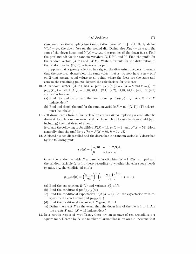
3.18 Problems 171

(We could use the sampling function notation here: W =∏

1.) Similarly, define

V (ω) = ω2, the down face on the second die. Define also X(ω) = ω1 + ω2, the

sum of the down faces, and Y (ω) = ω2ω2, the product of the down faces. Find

the pmf and cdf for the random variables X, Y, W , and V . Find the pmf’s for

the random vectors (X, Y ) and (W, V ). Write a formula for the distribution of

the random vector (W, V ) in terms of its pmf.

Suppose that a greedy scientist has rigged the dice using magnets to ensure

that the two dice always yield the same value; that is, we now have a new pmf

on Ω that assigns equal values to all points where the faces are the same and

zero to the remaining points. Repeat the calculations for this case.

10. A random vector (X, Y ) has a pmf pX,Y (k, j) = P (X = k and Y = j) of

pX,Y (k, j) = 1/8 if (k, j) = (0,3), (0,1), (2,1), (2,2), (4,0), (4,1), (4,2), or (4,3)

and is 0 otherwise.

(a) Find the pmf pY (y) and the conditional pmf pX|Y (x | y). Are X and Y

independent?

(b) Find and sketch the pmf for the random variable R = min(X, Y ). (The sketch

must be labeled.)

11. Jeff draws cards from a fair deck of 52 cards without replacing a card after he

draws it. Let the random variable X be the number of cards he draws until (and

including) the first draw of a heart.

Evaluate the following probabilities: P (X = 1). P (X = 2), and P (X = 52). More

generally, find the pmf for pX(k) = P (X = k), k = 1 . . . 52.

12. A biased 4 sided die is rolled and the down face is a random variable N described

by the following pmf:

pN (n) =

n/10 n = 1, 2, 3, 4

0 otherwise.

Given the random variable N a biased coin with bias (N + 1)/2N is flipped and

the random variable X is 1 or zero according to whether the coin shows heads

or tails, i.e., the conditional pmf is

pX|N(x|n) =

(n + 1

2n

)x (1 − n + 1

2n

)1−x

; x = 0, 1.

(a) Find the expectation E(N) and variance σ2N of N .

(b) Find the conditional pmf pN |X(n|x).

(c) Find the conditional expectation E(N |X = 1), i.e., the expectation with re-

spect to the conditional pmf pN |X(n|1).

(d) Find the conditional variance of N given X = 1.

(e) Define the event F as the event that the down face of the die is 1 or 4. Are

the events F and X = 1 independent?

13. In a certain region of west Texas, there are an average of ten armadillos per

square mile. Denote by N the number of armadillos in an area A. Assume that

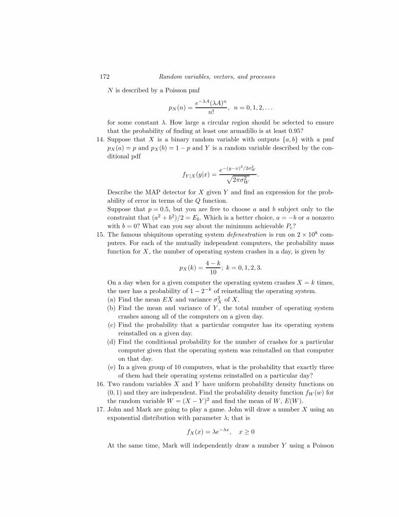
172 Random variables, vectors, and processes

N is described by a Poisson pmf

pN (n) =e−λA(λA)n

n!, n = 0, 1, 2, . . .

for some constant λ. How large a circular region should be selected to ensure

that the probability of finding at least one armadillo is at least 0.95?

14. Suppose that X is a binary random variable with outputs a, b with a pmf

pX(a) = p and pX(b) = 1 − p and Y is a random variable described by the con-

ditional pdf

fY |X(y|x) =e−(y−x)2/2σ2

W

√2πσ2

W

.

Describe the MAP detector for X given Y and find an expression for the prob-

ability of error in terms of the Q function.

Suppose that p = 0.5, but you are free to choose a and b subject only to the

constraint that (a2 + b2)/2 = Eb. Which is a better choice, a = −b or a nonzero

with b = 0? What can you say about the minimum achievable Pe?

15. The famous ubiquitous operating system defenestration is run on 2 × 108 com-

puters. For each of the mutually independent computers, the probability mass

function for X , the number of operating system crashes in a day, is given by

pX(k) =4 − k

10; k = 0, 1, 2, 3.

On a day when for a given computer the operating system crashes X = k times,

the user has a probability of 1 − 2−k of reinstalling the operating system.

(a) Find the mean EX and variance σ2X of X .

(b) Find the mean and variance of Y , the total number of operating system

crashes among all of the computers on a given day.

(c) Find the probability that a particular computer has its operating system

reinstalled on a given day.

(d) Find the conditional probability for the number of crashes for a particular

computer given that the operating system was reinstalled on that computer

on that day.

(e) In a given group of 10 computers, what is the probability that exactly three

of them had their operating systems reinstalled on a particular day?

16. Two random variables X and Y have uniform probability density functions on

(0, 1) and they are independent. Find the probability density function fW (w) for

the random variable W = (X − Y )2 and find the mean of W , E(W ).

17. John and Mark are going to play a game. John will draw a number X using an

exponential distribution with parameter λ; that is

fX(x) = λe−λx, x ≥ 0

At the same time, Mark will independently draw a number Y using a Poisson

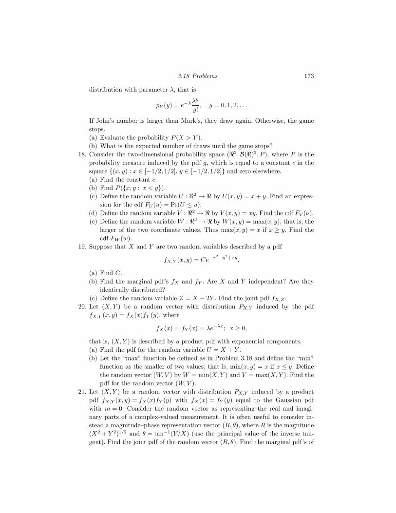
3.18 Problems 173

distribution with parameter λ, that is

pY (y) = e−λ λy

y!, y = 0, 1, 2, . . .

If John’s number is larger than Mark’s, they draw again. Otherwise, the game

stops.

(a) Evaluate the probability P (X > Y ).

(b) What is the expected number of draws until the game stops?

18. Consider the two-dimensional probability space (ℜ2,B(ℜ)2, P ), where P is the

probability measure induced by the pdf g, which is equal to a constant c in the

square (x, y) : x ∈ [−1/2, 1/2], y ∈ [−1/2, 1/2] and zero elsewhere.

(a) Find the constant c.

(b) Find P (x, y : x < y).(c) Define the random variable U : ℜ2 → ℜ by U(x, y) = x + y. Find an expres-

sion for the cdf FU (u) = Pr(U ≤ u).

(d) Define the random variable V : ℜ2 → ℜ by V (x, y) = xy. Find the cdf FV (ν).

(e) Define the random variable W : ℜ2 → ℜ by W (x, y) = max(x, y), that is, the

larger of the two coordinate values. Thus max(x, y) = x if x ≥ y. Find the

cdf FW (w).

19. Suppose that X and Y are two random variables described by a pdf

fX,Y (x, y) = Ce−x2−y2+xy.

(a) Find C.

(b) Find the marginal pdf’s fX and fY . Are X and Y independent? Are they

identically distributed?

(c) Define the random variable Z = X − 2Y . Find the joint pdf fX,Z .

20. Let (X, Y ) be a random vector with distribution PX,Y induced by the pdf

fX,Y (x, y) = fX(x)fY (y), where

fX(x) = fY (x) = λe−λx; x ≥ 0,

that is, (X, Y ) is described by a product pdf with exponential components.

(a) Find the pdf for the random variable U = X + Y .

(b) Let the “max” function be defined as in Problem 3.18 and define the “min”

function as the smaller of two values; that is, min(x, y) = x if x ≤ y. Define

the random vector (W, V ) by W = min(X, Y ) and V = max(X, Y ). Find the

pdf for the random vector (W, V ).

21. Let (X, Y ) be a random vector with distribution PX,Y induced by a product

pdf fX,Y (x, y) = fX(x)fY (y) with fX(x) = fY (y) equal to the Gaussian pdf

with m = 0. Consider the random vector as representing the real and imagi-

nary parts of a complex-valued measurement. It is often useful to consider in-

stead a magnitude–phase representation vector (R, θ), where R is the magnitude

(X2 + Y 2)1/2 and θ = tan−1(Y/X) (use the principal value of the inverse tan-

gent). Find the joint pdf of the random vector (R, θ). Find the marginal pdf’s of

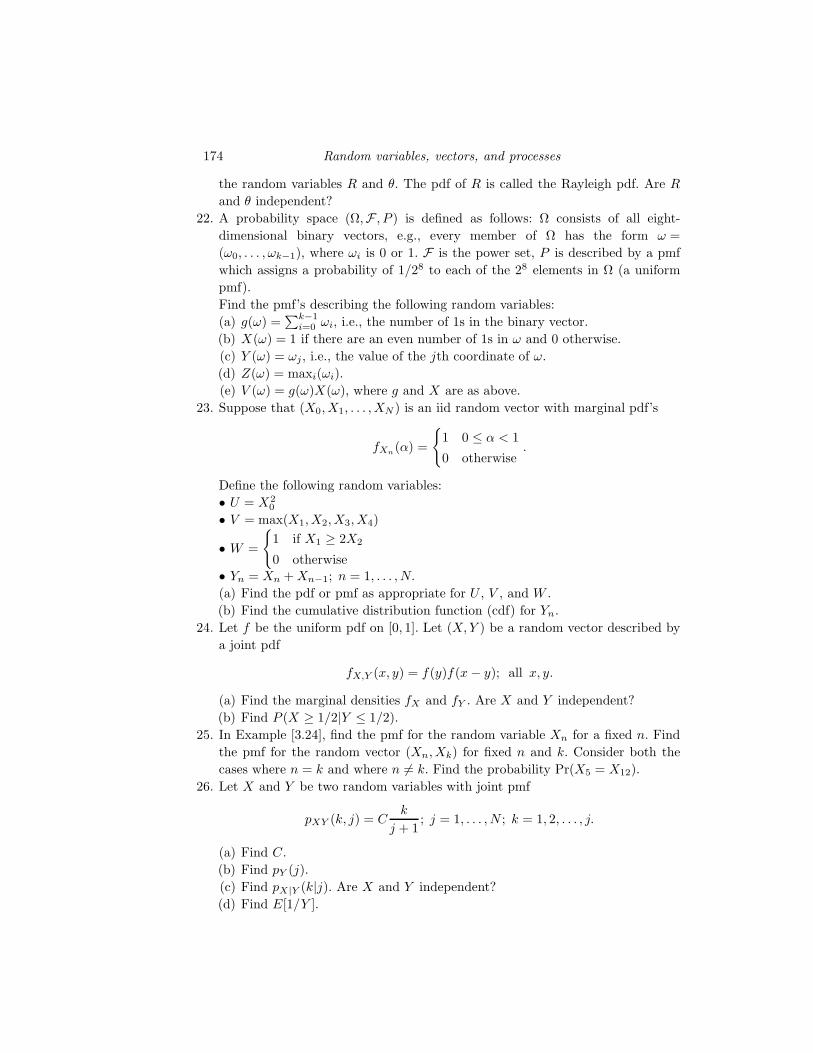
174 Random variables, vectors, and processes

the random variables R and θ. The pdf of R is called the Rayleigh pdf. Are R

and θ independent?

22. A probability space (Ω,F , P ) is defined as follows: Ω consists of all eight-

dimensional binary vectors, e.g., every member of Ω has the form ω =

(ω0, . . . , ωk−1), where ωi is 0 or 1. F is the power set, P is described by a pmf

which assigns a probability of 1/28 to each of the 28 elements in Ω (a uniform

pmf).

Find the pmf’s describing the following random variables:

(a) g(ω) =∑k−1

i=0 ωi, i.e., the number of 1s in the binary vector.

(b) X(ω) = 1 if there are an even number of 1s in ω and 0 otherwise.

(c) Y (ω) = ωj, i.e., the value of the jth coordinate of ω.

(d) Z(ω) = maxi(ωi).

(e) V (ω) = g(ω)X(ω), where g and X are as above.

23. Suppose that (X0, X1, . . . , XN ) is an iid random vector with marginal pdf’s

fXn(α) =

1 0 ≤ α < 1

0 otherwise.

Define the following random variables:

• U = X20

• V = max(X1, X2, X3, X4)

• W =

1 if X1 ≥ 2X2

0 otherwise• Yn = Xn + Xn−1; n = 1, . . . , N.

(a) Find the pdf or pmf as appropriate for U , V , and W .

(b) Find the cumulative distribution function (cdf) for Yn.

24. Let f be the uniform pdf on [0, 1]. Let (X, Y ) be a random vector described by

a joint pdf

fX,Y (x, y) = f(y)f(x − y); all x, y.

(a) Find the marginal densities fX and fY . Are X and Y independent?

(b) Find P (X ≥ 1/2|Y ≤ 1/2).

25. In Example [3.24], find the pmf for the random variable Xn for a fixed n. Find

the pmf for the random vector (Xn, Xk) for fixed n and k. Consider both the

cases where n = k and where n 6= k. Find the probability Pr(X5 = X12).

26. Let X and Y be two random variables with joint pmf

pXY (k, j) = Ck

j + 1; j = 1, . . . , N ; k = 1, 2, . . . , j.

(a) Find C.

(b) Find pY (j).

(c) Find pX|Y (k|j). Are X and Y independent?

(d) Find E[1/Y ].

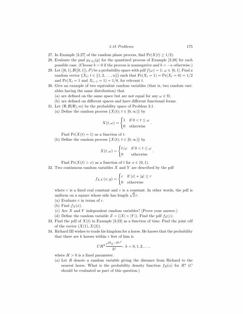
3.18 Problems 175

27. In Example [3.27] of the random phase process, find Pr(X(t) ≥ 1/2).

28. Evaluate the pmf pY (t)(y) for the quantized process of Example [3.28] for each

possible case. (Choose b = 0 if the process is nonnegative and b = −a otherwise.)

29. Let ([0, 1],B([0, 1]), P ) be a probability space with pdf f(ω) = 1; ω ∈ [0, 1]. Find a

random vector Xt; t ∈ 1, 2, . . . , n such that Pr(Xt = 1) = Pr(Xt = 0) = 1/2

and Pr(Xt = 1 and Xt−1 = 1) = 1/8, for relevant t.

30. Give an example of two equivalent random variables (that is, two random vari-

ables having the same distribution) that

(a) are defined on the same space but are not equal for any ω ∈ Ω,

(b) are defined on different spaces and have different functional forms.

31. Let (ℜ,B(ℜ), m) be the probability space of Problem 3.1.

(a) Define the random process X(t); t ∈ [0,∞) by

X(t, ω) =

1 if 0 < t ≤ ω

0 otherwise.

Find Pr(X(t) = 1) as a function of t.

(b) Define the random process X(t); t ∈ [0,∞) by

X(t, ω) =

t/ω if 0 < t ≤ ω

0 otherwise.

Find Pr(X(t) > x) as a function of t for x ∈ (0, 1).

32. Two continuous random variables X and Y are described by the pdf

fX,Y (x, y) =

c if |x| + |y| ≤ r

0 otherwise

where r is a fixed real constant and c is a constant. In other words, the pdf is

uniform on a square whose side has length√

2 r.

(a) Evaluate c in terms of r.

(b) Find fX(x).

(c) Are X and Y independent random variables? (Prove your answer.)

(d) Define the random variable Z = (|X | + |Y |). Find the pdf fZ(z).

33. Find the pdf of X(t) in Example [3.23] as a function of time. Find the joint cdf

of the vector (X(1), X(2)).

34. Richard III wishes to trade his kingdom for a horse. He knows that the probability

that there are k horses within r feet of him is

CHk r2ke−Hr2

k!; k = 0, 1, 2, . . . ,

where H > 0 is a fixed parameter.

(a) Let R denote a random variable giving the distance from Richard to the

nearest horse. What is the probability density function fR(α) for R? (C

should be evaluated as part of this question.)

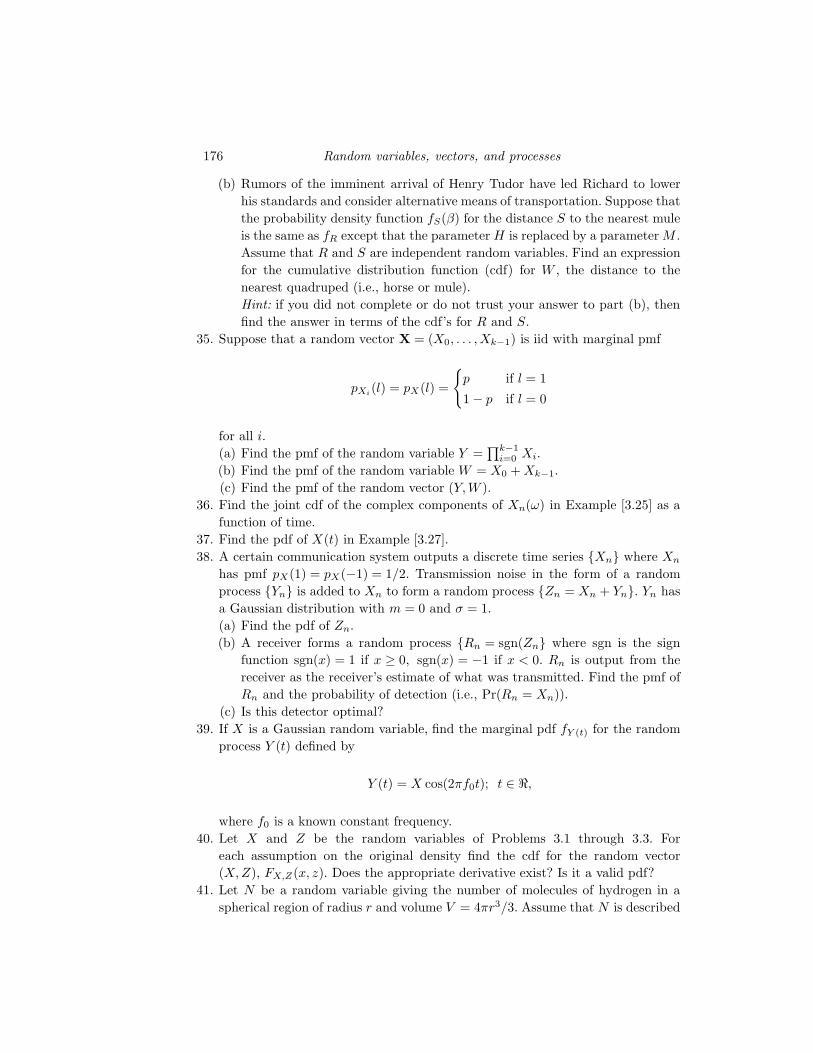
176 Random variables, vectors, and processes

(b) Rumors of the imminent arrival of Henry Tudor have led Richard to lower

his standards and consider alternative means of transportation. Suppose that

the probability density function fS(β) for the distance S to the nearest mule

is the same as fR except that the parameter H is replaced by a parameter M .

Assume that R and S are independent random variables. Find an expression

for the cumulative distribution function (cdf) for W , the distance to the

nearest quadruped (i.e., horse or mule).

Hint: if you did not complete or do not trust your answer to part (b), then

find the answer in terms of the cdf’s for R and S.

35. Suppose that a random vector X = (X0, . . . , Xk−1) is iid with marginal pmf

pXi(l) = pX(l) =

p if l = 1

1 − p if l = 0

for all i.

(a) Find the pmf of the random variable Y =∏k−1

i=0 Xi.

(b) Find the pmf of the random variable W = X0 + Xk−1.

(c) Find the pmf of the random vector (Y, W ).

36. Find the joint cdf of the complex components of Xn(ω) in Example [3.25] as a

function of time.

37. Find the pdf of X(t) in Example [3.27].

38. A certain communication system outputs a discrete time series Xn where Xn

has pmf pX(1) = pX(−1) = 1/2. Transmission noise in the form of a random

process Yn is added to Xn to form a random process Zn = Xn + Yn. Yn has

a Gaussian distribution with m = 0 and σ = 1.

(a) Find the pdf of Zn.

(b) A receiver forms a random process Rn = sgn(Zn where sgn is the sign

function sgn(x) = 1 if x ≥ 0, sgn(x) = −1 if x < 0. Rn is output from the

receiver as the receiver’s estimate of what was transmitted. Find the pmf of

Rn and the probability of detection (i.e., Pr(Rn = Xn)).

(c) Is this detector optimal?

39. If X is a Gaussian random variable, find the marginal pdf fY (t) for the random

process Y (t) defined by

Y (t) = X cos(2πf0t); t ∈ ℜ,

where f0 is a known constant frequency.

40. Let X and Z be the random variables of Problems 3.1 through 3.3. For

each assumption on the original density find the cdf for the random vector

(X, Z), FX,Z(x, z). Does the appropriate derivative exist? Is it a valid pdf?

41. Let N be a random variable giving the number of molecules of hydrogen in a

spherical region of radius r and volume V = 4πr3/3. Assume that N is described

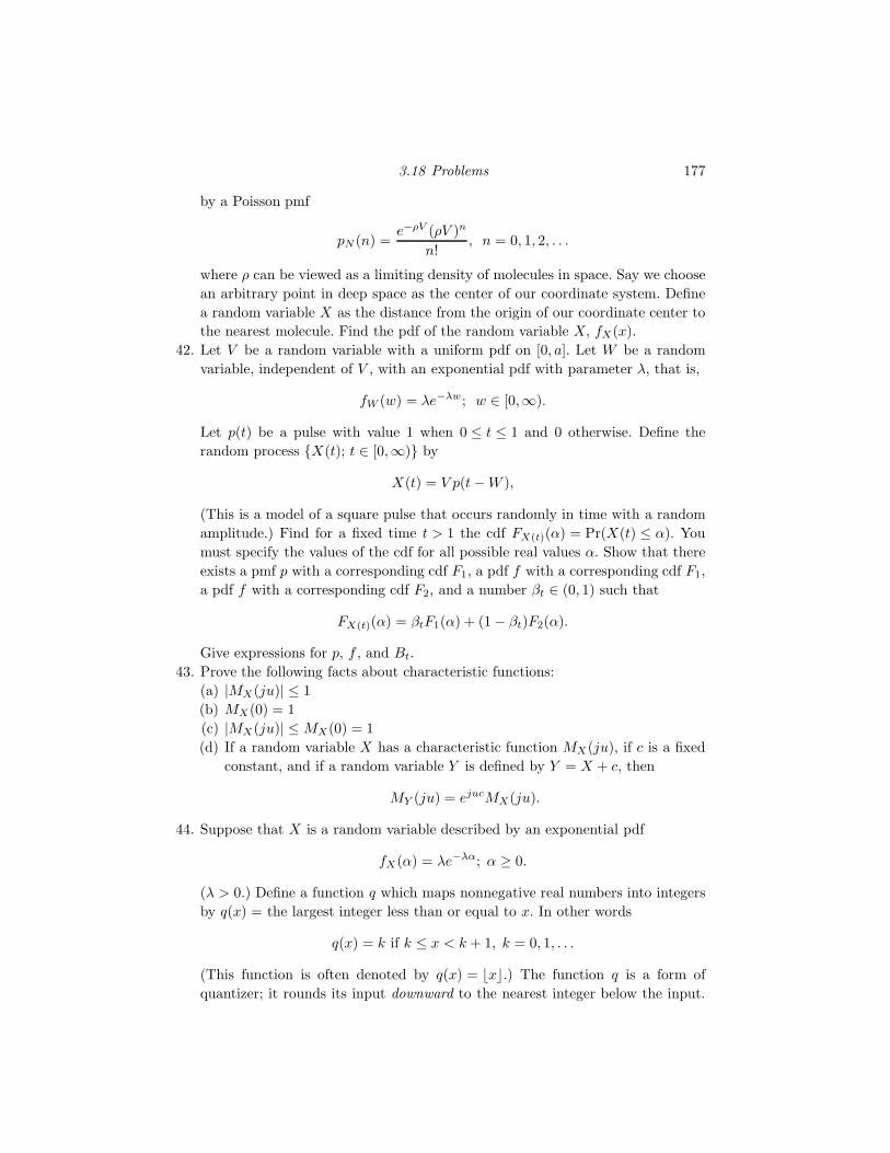
3.18 Problems 177

by a Poisson pmf

pN (n) =e−ρV (ρV )n

n!, n = 0, 1, 2, . . .

where ρ can be viewed as a limiting density of molecules in space. Say we choose

an arbitrary point in deep space as the center of our coordinate system. Define

a random variable X as the distance from the origin of our coordinate center to

the nearest molecule. Find the pdf of the random variable X, fX(x).

42. Let V be a random variable with a uniform pdf on [0, a]. Let W be a random

variable, independent of V , with an exponential pdf with parameter λ, that is,

fW (w) = λe−λw ; w ∈ [0,∞).

Let p(t) be a pulse with value 1 when 0 ≤ t ≤ 1 and 0 otherwise. Define the

random process X(t); t ∈ [0,∞) by

X(t) = V p(t − W ),

(This is a model of a square pulse that occurs randomly in time with a random

amplitude.) Find for a fixed time t > 1 the cdf FX(t)(α) = Pr(X(t) ≤ α). You

must specify the values of the cdf for all possible real values α. Show that there

exists a pmf p with a corresponding cdf F1, a pdf f with a corresponding cdf F1,

a pdf f with a corresponding cdf F2, and a number βt ∈ (0, 1) such that

FX(t)(α) = βtF1(α) + (1 − βt)F2(α).

Give expressions for p, f , and Bt.

43. Prove the following facts about characteristic functions:

(a) |MX(ju)| ≤ 1

(b) MX(0) = 1

(c) |MX(ju)| ≤ MX(0) = 1

(d) If a random variable X has a characteristic function MX(ju), if c is a fixed

constant, and if a random variable Y is defined by Y = X + c, then

MY (ju) = ejucMX(ju).

44. Suppose that X is a random variable described by an exponential pdf

fX(α) = λe−λα; α ≥ 0.

(λ > 0.) Define a function q which maps nonnegative real numbers into integers

by q(x) = the largest integer less than or equal to x. In other words

q(x) = k if k ≤ x < k + 1, k = 0, 1, . . .

(This function is often denoted by q(x) = ⌊x⌋.) The function q is a form of

quantizer; it rounds its input downward to the nearest integer below the input.

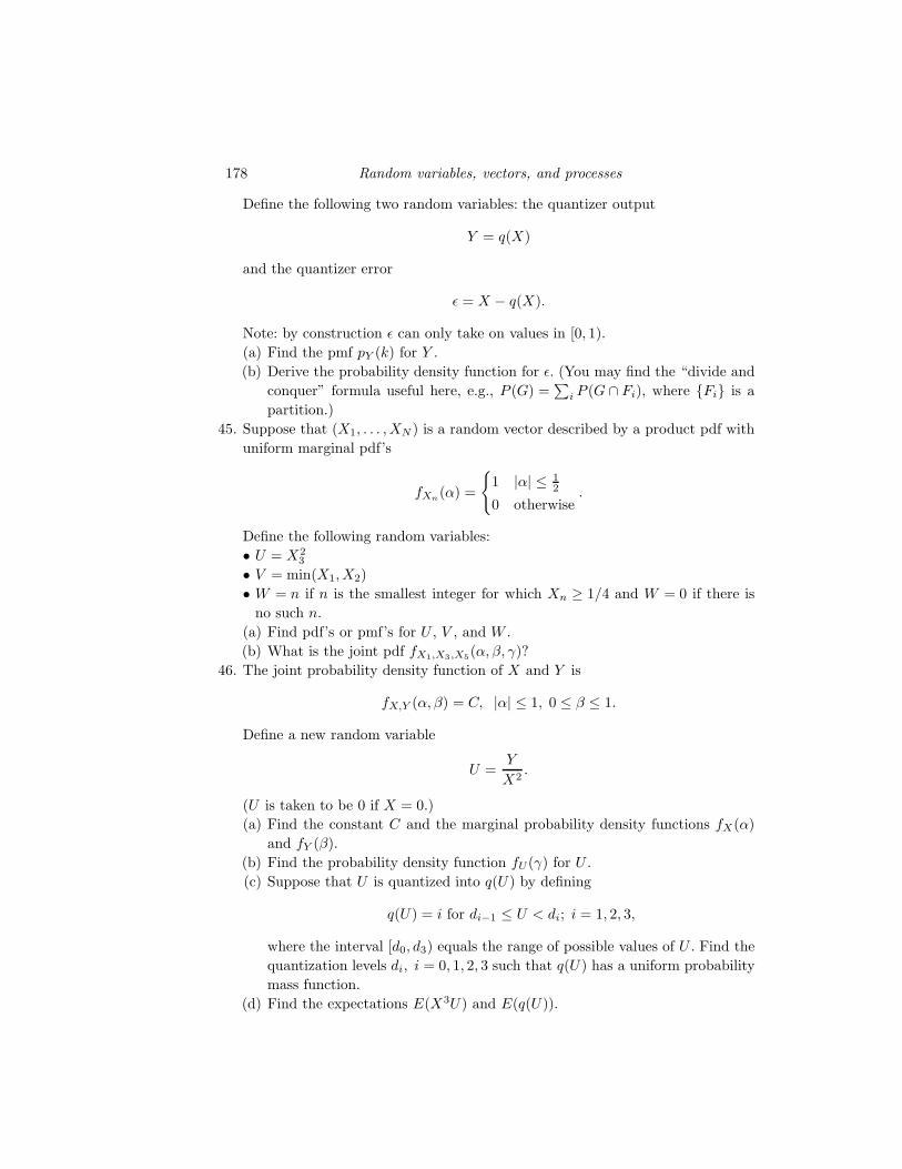
178 Random variables, vectors, and processes

Define the following two random variables: the quantizer output

Y = q(X)

and the quantizer error

ǫ = X − q(X).

Note: by construction ǫ can only take on values in [0, 1).

(a) Find the pmf pY (k) for Y .

(b) Derive the probability density function for ǫ. (You may find the “divide and

conquer” formula useful here, e.g., P (G) =∑

i P (G ∩ Fi), where Fi is a

partition.)

45. Suppose that (X1, . . . , XN ) is a random vector described by a product pdf with

uniform marginal pdf’s

fXn(α) =

1 |α| ≤ 1

2

0 otherwise.

Define the following random variables:

• U = X23

• V = min(X1, X2)

• W = n if n is the smallest integer for which Xn ≥ 1/4 and W = 0 if there is

no such n.

(a) Find pdf’s or pmf’s for U , V , and W .

(b) What is the joint pdf fX1,X3,X5(α, β, γ)?

46. The joint probability density function of X and Y is

fX,Y (α, β) = C, |α| ≤ 1, 0 ≤ β ≤ 1.

Define a new random variable

U =Y

X2.

(U is taken to be 0 if X = 0.)

(a) Find the constant C and the marginal probability density functions fX(α)

and fY (β).

(b) Find the probability density function fU (γ) for U .

(c) Suppose that U is quantized into q(U) by defining

q(U) = i for di−1 ≤ U < di; i = 1, 2, 3,

where the interval [d0, d3) equals the range of possible values of U . Find the

quantization levels di, i = 0, 1, 2, 3 such that q(U) has a uniform probability

mass function.

(d) Find the expectations E(X3U) and E(q(U)).

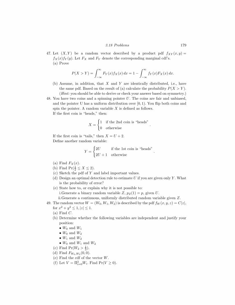
3.18 Problems 179

47. Let (X, Y ) be a random vector described by a product pdf fXY (x, y) =

fX(x)fY (y). Let FX and FY denote the corresponding marginal cdf’s.

(a) Prove

P (X > Y ) =

∫ ∞

−∞FY (x)fX(x) dx = 1 −

∫ ∞

−∞fY (x)FX (x) dx.

(b) Assume, in addition, that X and Y are identically distributed, i.e., have

the same pdf. Based on the result of (a) calculate the probability P (X > Y ).

(Hint: you should be able to derive or check your answer based on symmetry.)

48. You have two coins and a spinning pointer U . The coins are fair and unbiased,

and the pointer U has a uniform distribution over [0, 1). You flip both coins and

spin the pointer. A random variable X is defined as follows.

If the first coin is “heads,” then:

X =

1 if the 2nd coin is “heads”

0 otherwise.

If the first coin is “tails,” then X = U + 2.

Define another random variable:

Y =

2U if the 1st coin is “heads”

2U + 1 otherwise.

(a) Find FX(x).

(b) Find Pr(12 ≤ X ≤ 2).

(c) Sketch the pdf of Y and label important values.

(d) Design an optimal detection rule to estimate U if you are given only Y . What

is the probability of error?

(e) State how to, or explain why it is not possible to:

i.Generate a binary random variable Z, pZ(1) = p, given U .

ii.Generate a continuous, uniformly distributed random variable given Z.

49. The random vector W = (W0, W1, W2) is described by the pdf fW (x, y, z) = C|z|,for x2 + y2 ≤ 1, |z| ≤ 1.

(a) Find C.

(b) Determine whether the following variables are independent and justify your

position:

• W0 and W1

• W0 and W2

• W1 and W2

• W0 and W1 and W2

(c) Find Pr(W2 > 13 ).

(d) Find FW0,W2(0, 0).

(e) Find the cdf of the vector W .

(f) Let V = Π2i=0Wi. Find Pr(V ≥ 0).

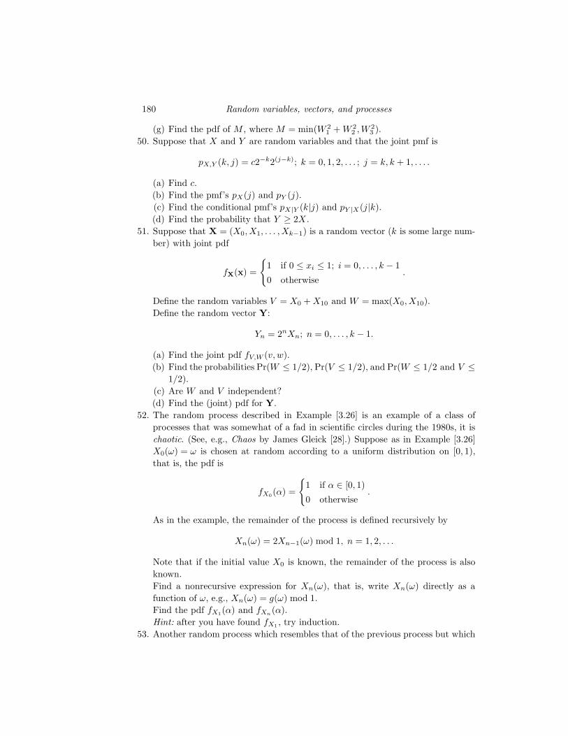
180 Random variables, vectors, and processes

(g) Find the pdf of M , where M = min(W 21 + W 2

2 , W 23 ).

50. Suppose that X and Y are random variables and that the joint pmf is

pX,Y (k, j) = c2−k2(j−k); k = 0, 1, 2, . . . ; j = k, k + 1, . . . .

(a) Find c.

(b) Find the pmf’s pX(j) and pY (j).

(c) Find the conditional pmf’s pX|Y (k|j) and pY |X(j|k).

(d) Find the probability that Y ≥ 2X .

51. Suppose that X = (X0, X1, . . . , Xk−1) is a random vector (k is some large num-

ber) with joint pdf

fX(x) =

1 if 0 ≤ xi ≤ 1; i = 0, . . . , k − 1

0 otherwise.

Define the random variables V = X0 + X10 and W = max(X0, X10).

Define the random vector Y:

Yn = 2nXn; n = 0, . . . , k − 1.

(a) Find the joint pdf fV,W (v, w).

(b) Find the probabilities Pr(W ≤ 1/2), Pr(V ≤ 1/2), and Pr(W ≤ 1/2 and V ≤1/2).

(c) Are W and V independent?

(d) Find the (joint) pdf for Y.

52. The random process described in Example [3.26] is an example of a class of

processes that was somewhat of a fad in scientific circles during the 1980s, it is

chaotic. (See, e.g., Chaos by James Gleick [28].) Suppose as in Example [3.26]

X0(ω) = ω is chosen at random according to a uniform distribution on [0, 1),

that is, the pdf is

fX0(α) =

1 if α ∈ [0, 1)

0 otherwise.

As in the example, the remainder of the process is defined recursively by

Xn(ω) = 2Xn−1(ω) mod 1, n = 1, 2, . . .

Note that if the initial value X0 is known, the remainder of the process is also

known.

Find a nonrecursive expression for Xn(ω), that is, write Xn(ω) directly as a

function of ω, e.g., Xn(ω) = g(ω) mod 1.

Find the pdf fX1(α) and fXn(α).

Hint: after you have found fX1 , try induction.

53. Another random process which resembles that of the previous process but which

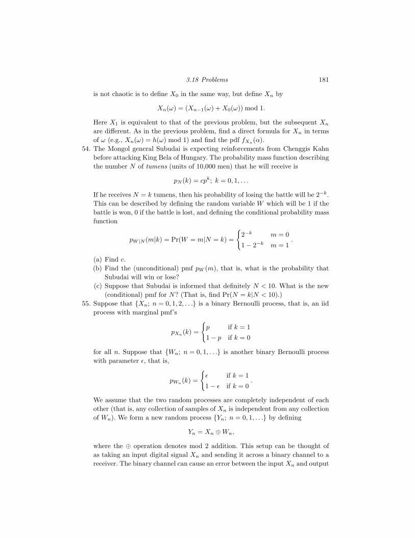
3.18 Problems 181

is not chaotic is to define X0 in the same way, but define Xn by

Xn(ω) = (Xn−1(ω) + X0(ω)) mod 1.

Here X1 is equivalent to that of the previous problem, but the subsequent Xn

are different. As in the previous problem, find a direct formula for Xn in terms

of ω (e.g., Xn(ω) = h(ω) mod 1) and find the pdf fXn(α).

54. The Mongol general Subudai is expecting reinforcements from Chenggis Kahn

before attacking King Bela of Hungary. The probability mass function describing

the number N of tumens (units of 10,000 men) that he will receive is

pN (k) = cpk; k = 0, 1, . . .

If he receives N = k tumens, then his probability of losing the battle will be 2−k.

This can be described by defining the random variable W which will be 1 if the

battle is won, 0 if the battle is lost, and defining the conditional probability mass

function

pW |N (m|k) = Pr(W = m|N = k) =

2−k m = 0

1 − 2−k m = 1.

(a) Find c.

(b) Find the (unconditional) pmf pW (m), that is, what is the probability that

Subudai will win or lose?

(c) Suppose that Subudai is informed that definitely N < 10. What is the new

(conditional) pmf for N? (That is, find Pr(N = k|N < 10).)

55. Suppose that Xn; n = 0, 1, 2, . . . is a binary Bernoulli process, that is, an iid

process with marginal pmf’s

pXn(k) =

p if k = 1

1 − p if k = 0

for all n. Suppose that Wn; n = 0, 1, . . . is another binary Bernoulli process

with parameter ǫ, that is,

pWn(k) =

ǫ if k = 1

1 − ǫ if k = 0.

We assume that the two random processes are completely independent of each

other (that is, any collection of samples of Xn is independent from any collection

of Wn). We form a new random process Yn; n = 0, 1, . . . by defining

Yn = Xn ⊕ Wn,

where the ⊕ operation denotes mod 2 addition. This setup can be thought of

as taking an input digital signal Xn and sending it across a binary channel to a

receiver. The binary channel can cause an error between the input Xn and output

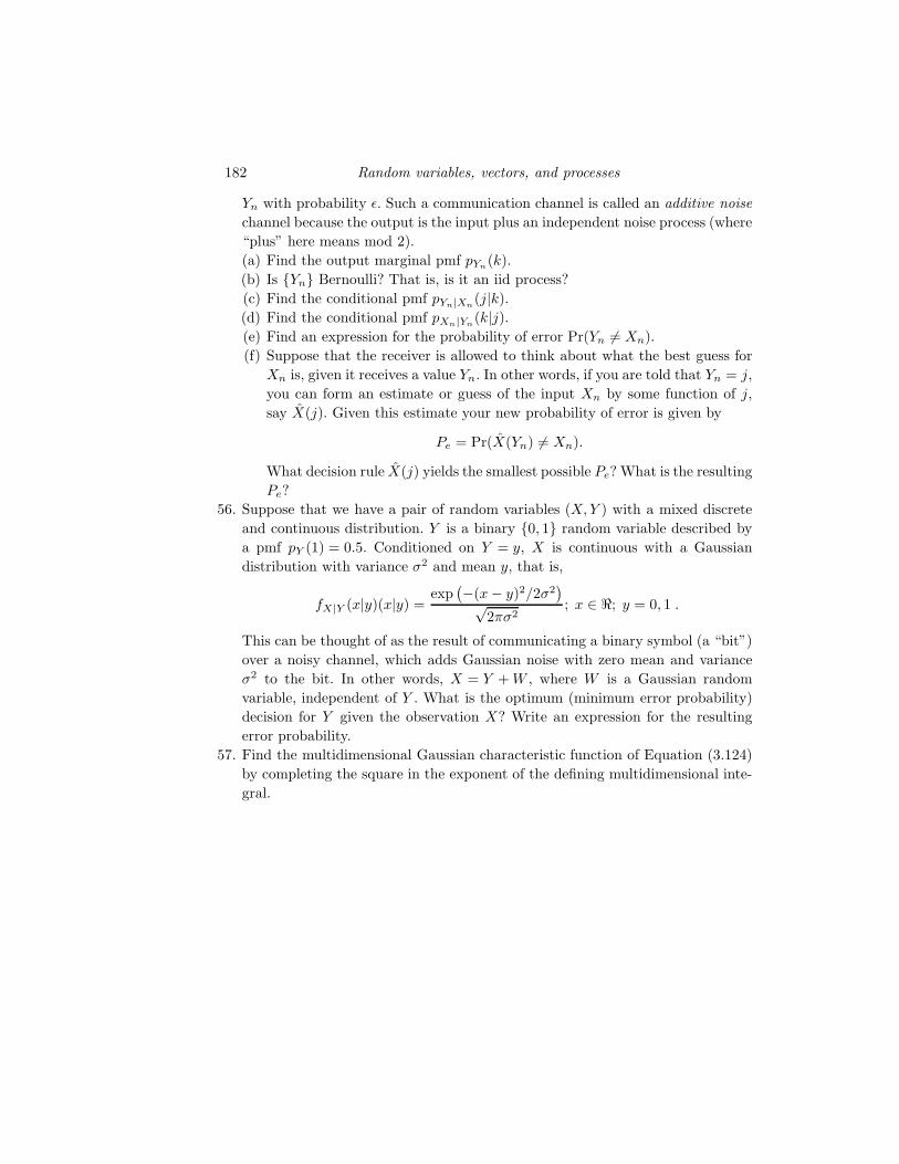
182 Random variables, vectors, and processes

Yn with probability ǫ. Such a communication channel is called an additive noise

channel because the output is the input plus an independent noise process (where

“plus” here means mod 2).

(a) Find the output marginal pmf pYn(k).

(b) Is Yn Bernoulli? That is, is it an iid process?

(c) Find the conditional pmf pYn|Xn(j|k).

(d) Find the conditional pmf pXn|Yn(k|j).

(e) Find an expression for the probability of error Pr(Yn 6= Xn).

(f) Suppose that the receiver is allowed to think about what the best guess for

Xn is, given it receives a value Yn. In other words, if you are told that Yn = j,

you can form an estimate or guess of the input Xn by some function of j,

say X(j). Given this estimate your new probability of error is given by

Pe = Pr(X(Yn) 6= Xn).

What decision rule X(j) yields the smallest possible Pe? What is the resulting

Pe?

56. Suppose that we have a pair of random variables (X, Y ) with a mixed discrete

and continuous distribution. Y is a binary 0, 1 random variable described by

a pmf pY (1) = 0.5. Conditioned on Y = y, X is continuous with a Gaussian

distribution with variance σ2 and mean y, that is,

fX|Y (x|y)(x|y) =exp

(−(x − y)2/2σ2

)√

2πσ2; x ∈ ℜ; y = 0, 1 .

This can be thought of as the result of communicating a binary symbol (a “bit”)

over a noisy channel, which adds Gaussian noise with zero mean and variance

σ2 to the bit. In other words, X = Y + W , where W is a Gaussian random

variable, independent of Y . What is the optimum (minimum error probability)

decision for Y given the observation X? Write an expression for the resulting

error probability.

57. Find the multidimensional Gaussian characteristic function of Equation (3.124)

by completing the square in the exponent of the defining multidimensional inte-

gral.

4

Expectation and averages

4.1 Averages

In engineering practice we are often interested in the average behavior of

measurements on random processes. The goal of this chapter is to link the

two distinct types of averages that are used – long-term time averages taken

by calculations on an actual physical realization of a random process and

averages calculated theoretically by probabilistic calculus at some given in-

stant of time, averages that are called expectations. As we shall see, both

computations often (but by no means always) give the same answer. Such

results are called laws of large numbers or ergodic theorems.

At first glance from a conceptual point of view, it seems unlikely that

long-term time averages and instantaneous probabilistic averages would be

the same. If we take a long-term time average of a particular realization of

the random process, say X(t, ω0); t ∈ T , we are averaging for a particular

ω which we cannot know or choose; we do not use probability in any way

and we are ignoring what happens with other values of ω. Here the averages

are computed by summing the sequence or integrating the waveform over t

while ω0 stays fixed. If, on the other hand, we take an instantaneous prob-

abilistic average, say at the time t0, we are taking a probabilistic average

and summing or integrating over ω for the random variable X(t0, ω). Thus

we have two averages, one along the time axis with ω fixed, the other along

the ω axis with time fixed. It seems that there should be no reason for the

answers to agree. Taking a more practical point of view, however, it seems

that the time and probabilistic averages must be the same in many situa-

tions. For example, suppose that you measure the percentage of time that a

particular noise voltage exceeds 10 volts. If you make the measurement over

a sufficiently long period of time, the result should be a reasonably good

183

184 Expectation and averages

estimate of the probability that the noise voltage exceeds 10 volts at any

given instant of time – a probabilistic average value.

To proceed further, for simplicity we concentrate on a random process

with discrete alphabet and discrete time. Other cases are considered by

converting appropriate sums into integrals. Let Xn be an arbitrary discrete

alphabet, discrete time process. Since the process is random, we cannot

predict accurately its instantaneous or short-term behavior – we can only

make probabilistic statements. Based on experience with coins, dice, and

roulette wheels, however, one expects that the long-term average behavior

can be characterized with more accuracy. For example, if one flips a fair coin,

short sequences of flips are unpredictable. However, if one flips long enough,

one would expect to have an average of about 50% of the flips result in heads.

This is a time average of an instantaneous function of a random process –

a type of counting function that we will consider extensively. It is obvious

that there are many functions that we can average: the average value, the

average power, etc. We will proceed by defining one particular average, the

value of the sample average of a random process, which is formulated as

Sn = n−1n−1∑

i=0

Xi; n = 1, 2, 3, . . .

We will investigate the behavior of Sn for large n, i.e., for a long-term time

average. Thus, for example, if the random process Xn is the coin-flipping

model, the binary process with alphabet 0, 1, then Sn is the number of 1s

divided by the total number of flips – the fraction of flips that produced a

1. As noted before, Sn should be close to 50% for large n if the coin is fair.

Note that, as in Example [3.7], for each n, Sn is a random variable that

is defined on the same probability space as the random process Xn. This

is made explicit by writing the ω dependence:

Sn(ω) =1

n

n−1∑

k=0

Xk(ω).

In more direct analogy to Example [3.7], we can consider the Xn as co-

ordinate functions on a sequence space, say (ℜZ ,B(ℜZ),m), where m is

the distribution of the process, in which case Sn is defined directly on the

sequence space. The form of definition is simply a matter of semantics or

convenience. Observe, however, that in any case Sn; n = 1, 2, . . . is itself

a random process since it is an indexed family of random variables defined

on a probability space.

For the discrete alphabet random process that we are considering, we can

4.1 Averages 185

rewrite the sum in another form by grouping together all equal terms:

Sn(ω) =∑

a∈A

ar(n)a (ω) (4.1)

where A is the range space of the discrete alphabet random variable Xn

and r(n)a (ω) = n−1 [number of occurrences of the letter a in Xi(ω), i =

0, 1, 2, . . . , n − 1]. The random variable r(n)a is called the nth-order relative

frequency of the symbol a. For the binary coin-flipping example we have

considered, A = 0, 1, and Sn(ω) = r(n)1 (ω), the average number of heads

in the first n flips. In other words, for the binary coin-flipping example, the

sample average and the relative frequency of heads are the same quantity.

More generally, the reader should note that r(n)a can always be written as

the sample average of the indicator function for a, 1a(x):

r(n)a = n−1

n−1∑

i=0

1a(Xi),

where

1a(x) =

1 if x = a

0 otherwise.

Note that 1a is a more precise, but more clumsy, notation for the indicator

function of the singleton set a. We shall use the shorter form here.

Let us now assume that all of the marginal pmf’s of the given process are

the same, say pX(x), x ∈ A. Based on intuition and gambling experience,

one might suspect that as n goes to infinity, the relative frequency of a

symbol a should go to its probability of occurrence, pX(a). To continue the

example of binary coin-flipping, the relative frequency of heads in n tosses

of a fair coin should tend to 1/2 as n → ∞. If these statements are true,

that is, if in some sense,

r(n)a →

n→∞pX(a), (4.2)

then it follows that in a similar sense

Sn →n→∞

∑

a∈A

apX(a), (4.3)

the same expression as (4.1) with the relative frequency replaced by the

pmf. The formula on the right is an example of an expectation of a random

variable, a weighted average with respect to a probability measure. The

formula should be recognized as a special case of the definition of expectation

186 Expectation and averages

of (2.34), where the pmf is pX and g(x) = x, the identity function. The

previous plausibility argument motivates the study of such weighted averages

because they will characterize the limiting behavior of time averages in the

same way that probabilities characterize the limiting behavior of relative

frequencies.

Limiting statements of the form of (4.2) and (4.3) are called laws of large

numbers or ergodic theorems. They relate long-run sample averages or time-

average behavior to probabilistic calculations made at any given instant of

time. It is obvious that such laws or theorems do not always hold. If the coin

we are flipping wears in a known fashion with time so that the probability

of a head changes, then one could hardly expect that the relative frequency

of heads would equal the probability of heads at time zero.

In order to make precise statements and to develop conditions under

which the laws of theorems do hold, we first need to develop the prop-

erties of the quantity on the right-hand side of (4.2) and (4.3). In par-

ticular, we cannot at this point make any sense out of a statement like

“limn→∞ Sn =∑

a∈AapX(a),” since we have no definition for such a limit of

random variables or functions of random variables. It is obvious, however,

that the usual definition of a limit used in calculus will not do, because Sn is

a random variable albeit a random variable whose “randomness” decreases

in some sense with increasing n. Thus the limit must be defined in some

fashion that involves probability. Such limits are deferred to a later section.

We begin by looking at the definitions and calculus of expectations.

4.2 Expectation

Given a discrete alphabet random variable X specified by a pmf pX , define

the expected value, probabilistic average, or mean of X by

E(X) =∑

x∈A

xpX(x). (4.4)

The expectation is also denoted by EX or E[X] or by an overbar, as

X . The expectation is also sometimes called an ensemble average to denote

averaging across the ensemble of sequences that is generated for different

values of ω at a given instant of time.

The astute reader might note that we have really provided two definitions

of the expectation of X. The definition of (4.4) has already been noted to be

a special case of (2.34) with pmf pX and function g(x) = x. Alternatively,

we could use (2.34) in a more fundamental form and consider g(ω) = X(ω)

is a function defined on an underlying probability space described by a pmf

4.2 Expectation 187

p or a pdf f , in which case (2.34) or (2.57) provide a different formula for

finding the expectation in terms of the original probability function:

E(X) =∑

ω

X(ω)p(ω) (4.5)

if the original space is discrete, or

E(X) =

∫X(r)f(r) dr (4.6)

if it is continuous. Are these two versions consistent? The answer is yes,

as will be proved soon by the fundamental theorem of expectation. The

equivalence of these forms is essentially a change of variables formula.

The mean of a random variable is a weighted average of the possible values

of the random variable with the pmf used as a weighting. Before continuing,

observe that we can define an analogous quantity for a continuous random

variable possessing a pdf: if the random variable X is described by a pdf fX ,

then we define the expectation of X by

EX =

∫xfX(x) dx, (4.7)

where we have replaced the sum by an integral. Analogous to the discrete

case, this formula is a special case of (2.57) with pdf f = fX and g being

the identity function. We can also use (2.57) to express the expectation in

terms of an underlying pdf, say f , as

EX =

∫X(r)f(r) dr.

The equivalence of these two formulas will be considered when the funda-

mental theorem of expectation is treated.

Although the integral does not have the intuitive motivation involving a

relative frequency converging to a pmf that the earlier sum did, we shall

see that it plays the analogous role in the laws of large numbers. Roughly

speaking, this is because continuous random variables can be approximated

by discrete random variables arbitrarily closely by very fine quantization.

Through this procedure, the integrals with pdf’s are approximated by sums

with pmf’s and the discrete alphabet results imply the continuous alphabet

results by taking appropriate limits. Because of the direct analogy, we shall

develop the properties of expectations for continuous random variables along

with those for discrete alphabet random variables. Note in passing that,

analogous to using the Stieltjes integral as a unified notation for sums and

integrals when computing probabilities, the same thing can be done for

188 Expectation and averages

expectations. If FX is the cdf of a random variable X, define

EX =

∫x dFX(x) =

∑xxpX(x) if X discrete

∫xfX(x) dx if X has a pdf

.

In a similar manner, we can define the expectation of a mixture random

variable having both continuous and discrete parts in a manner analogous

to (3.36).

Examples The following examples provide some typical expectation compu-

tations.

[4.1] As a slight generalization of the fair coin flip, consider the more

general binary pmf with parameter p; that is, pX(1) = p and pX(0) =

1 − p. In this case

EX =1∑

i=0

xpX(x) = 0(1 − p) + 1p = p.

It is interesting to note that in this example, as is generally true for

discrete random variables, EX is not necessarily in the alphabet of the

random variable, i.e., EX 6= 0 or 1 unless p = 0 or 1.

[4.2] A more complicated discrete example is a geometric random variable.

In this case

EX =

∞∑

k=1

kpX(k) =

∞∑

k=1

kp(1 − p)k−1,

a sum evaluated in (2.48) as 1/p.

[4.3] As an example of a continuous random variable, assume that X is

a uniform random variable on [0, 1], that is, its density is one on [0, 1].

Here

EX =

∫ 1

0xfX(x) dx =

∫ 1

0x dx =

1

2,

an integral evaluated in (2.67).

[4.4] If X is an exponential random variable with parameter λ, then from

(2.71)∫ ∞

0rλe−λr dr =

1

λ. (4.8)

4.3 Functions of random variables 189

In some cases expectations can be found virtually by inspection. For exam-

ple, if X has an even pdf fX – that is, if fX(−x) = fX(x) for all x ∈ ℜ –

then if the integral exists, EX = 0, since xfX(x) is an odd function and

hence has a zero integral. The assumption that the integral exists is nec-

essary because not all even functions are integrable. For example, suppose

that we have a pdf fX(x) = c/x2 for all |x| ≥ 1, where c is a normalization

constant. Then it is not true that EX is zero, even though the pdf is even,

because the Riemann integral∫

x: |x|≥1

x

x2dx

does not exist. (The puzzled reader should review the definition of indefinite

integrals. Their existence requires that the limit

limT→∞

limS→∞

∫ S

−TxfX(x) dx

exists regardless of how T and S tend to infinity; in particular, the existence

of the limit with the constraint T = S is not sufficient for the existence of

the integral. These limits do not exist for the given example because 1/x is

not integrable on [1,∞).) Nonetheless, it is convenient to set EX to 0 in

this example because of the obvious intuitive interpretation.

Sometimes the pdf is an even function about some nonzero value, that is,

fX(m + x) = fX(m − x), where m is some constant. In this case, it is easily

seen that if if the expectation exists, then EX = m, as the reader can quickly

verify by a change of variable in the integral defining the expectation. The

most important example of this is the Gaussian pdf, which is even about

the constant m.

The same conclusions also obviously hold for an even pmf.

4.3 Functions of random variables

In addition to the expectation of a given random variable, we will often be

interested in the expectations of other random variables formed as functions

of the given one. In the beginning of the chapter we introduced the relative

frequency function, r(n)a , which counts the relative number of occurrences

of the value a in a sequence of n terms. We are interested in its expected

value and in the expected value of the indicator function that appears in

the expression for r(n)a . More generally, given a random variable X and a

function g : ℜ → ℜ, we might wish to find the expectation of the random

variable Y = g(X). If X corresponds to a voltage measurement and g is

190 Expectation and averages

a simple squaring operation, g(X) = X2, then g(X) provides the instanta-

neous energy across a unit resistor. Its expected value, then, represents the

probabilistic average energy. More generally than the square of a random

variable, the moments of a random variable X are defined by E[Xk] for

k = 1, 2, . . .The mean is the first moment, the square is the second moment,

and so on. If the random variable is complex-valued, then often the absolute

moments E[|X|k] are of interest. Moments are often useful as general param-

eters of a distribution, providing information on its shape without requiring

the complete pdf or pmf. Some distributions are completely characterized by

a few moments (e.g., the Gaussian). It is often useful to consider moments of

a “centralized” random variable formed by removing its mean. The kth cen-

tralized moment is defined by E[(X − E(X))k ]. The kth centralized absolute

moment is defined by E[|X − E(X)|k ].

Of particular interest is the second centralized moment or variance σ2 ∆=

E[(X − E(X))2]. Other functions that are of interest are indicator functions

of a set, 1F (x) = 1 if x ∈ F and 0 otherwise, so that 1F (X) is a binary

random variable indicating whether or not the value of X lies in F , and

complex exponentials ejuX .

Expectations of functions of random variables were defined in this chap-

ter in terms of the derived distribution for the new random variable. In

chapter 3, however, they were defined in terms of the original pmf or pdf

in the underlying probability space, a formula not requiring that the new

distribution be derived. We next show that the two formulas are consistent.

First consider finding the expectation of Y by using derived distribution

techniques to find the probability function for Y . Then use the definition of

expectation to evaluate EY . Specifically, if X is discrete, the pmf for Y is

found as before as

pY (y) =∑

x: g(x)=y

pX(x), y ∈ AY .

EY is then found as

EY =∑

AY

ypY (y).

Although it is straightforward to find the probability function for Y , it can

be a nuisance if it is being found only as a step in the evaluation of the

expectation EY = Eg(X). A second and easier method of finding EY is

normally used. Looking at the formula for EX, it seems intuitively obvious

that E(g(X)) should result if x is replaced by g(x). This can be proved

by the following simple procedure. The expectation of Y is found directly

4.3 Functions of random variables 191

from the pmf for X by starting with the pmf for Y , then substituting for its

expression in terms of the pmf of X and reordering the summation:

EY =∑

AY

ypY (y) =∑

AY

y

∑

x: g(x)=y

pX(x)

=∑

AY

∑

x: g(x)=y

g(x)pX(x)

=∑

AX

g(x)pX (x).

This little bit of manipulation is given the fancy name of the fundamental

theorem of expectation. It is a very useful formula in that it allows one to

compute expectations of functions of random variables without needing to

perform the (usually more difficult) derived distribution operations.

A similar proof holds for the case of a discrete random variable defined

on a continuous probability space described by a pdf. The proof is left as an

exercise (Problem 4.4).

A similar change of variables argument with integrals in place of sums

yields the analogous pdf result for continuous random variables. As is cus-

tomary, however, we have only provided the proof for the simple discrete

case. For the details of the continuous case, we refer the reader to books

on integration or analysis. The reader should be aware that such integral

results will have additional technical assumptions (almost always satisfied)

required to guarantee the existence of the various integrals. We summarize

the results below.

Theorem 4.1 Fundamental theorem of expectation.

Let a random variable X be described by a cdf FX , which is in turn described

by either a pmf pX or a pdf fX . Given any measurable function g : ℜ → ℜ,

the resulting random variable Y = g(X) has expectation

EY = E(g(X)) =

∫y dFg(X)(y)

=

∫g(x) dFX =

∑xg(x)pX (x) if discrete with a pmf

∫xg(x)fX (x) dx if continuous with a pdf

.

The qualification “measurable” is needed in the theorem to guarantee the

existence of the expectation. Measurability is satisfied by almost any func-

tion that you can think of and, for all practical purposes, the requirement

can be neglected.

192 Expectation and averages

Examples As a simple example of the use of this formula, consider a random

variable X with a uniform pdf on [−1/2, 1/2]. Define the random variable

Y = X2, that is g(r) = r2. We can use the derived distribution formula (3.40)

to write

fY (y) = y−(1/2)fX

(y(1/2)

); y ≥ 0,

and hence

fY (y) = y−(1/2); y ∈ (0, 1/4],

where we have used the fact that fX(y(1/2)) is 1 only if the nonnegative

argument is less than (1/2) or y ≤ 14 . We can then find EY as

EY =

∫yfY (y) dy =

∫ 1/4

0y1/2 dy =

(1/4)3/2

3/2=

1

12.

Alternatively, we can use the theorem to write

EY = E(X2) =

∫ 1/2

−1/2x2 dx = 2

(1/2)3

3=

1

12.

Note that the result is the same for each method. However, the second

calculation is much simpler, especially if one considers the work that was

required in Chapter 3 to derive the density formula for the square of a

random variable.

[4.5] A second example generalizes an observation of Chapter 2 and shows

that expectations can be used to express probabilities (and hence that

probabilities can be considered as special cases of expectation). Recall

that the indicator function of an event F is defined by

1F (x) =

1 if x ∈ F

0 otherwise.

The probability of the event F can be written in the following form which

is convenient in certain computations:

E1F (X) =

∫1F (x) dFX (x) =

∫

FdFX(x) = PX(F ), (4.9)

where we have used the universal Stieltjes integral representation of

(3.32) to save writing out both sums of pmf’s and integrals of pdf’s

(the reader who is unconvinced by (4.9) should write out the specific

4.3 Functions of random variables 193

pmf and pdf forms). Observe also that finding probability by taking ex-

pectations of indicator functions is like finding a relative frequency by

taking a sample average of an indicator function.

It is obvious from the fundamental theorem of expectation that the expected

value of any function of a random value can be calculated from its probability

distribution. The preceding example demonstrates that the converse is also

true: the probability distribution can be calculated from a knowledge of the

expectation of a large enough set of functions of the random variable. The

example provides the result for the set of all indicator functions. The choice

is not unique, as shown by the following example.

[4.6] Let g(x) be the complex function ejux where u is an arbitrary con-

stant. For a cdf FX , define

E(g(X)) = E(ejuX) =

∫ejux dFX(x).

This expectation is immediately recognizable as the characteristic func-

tion of the random variable (or its distribution), providing a shorthand

definition

MX(ju) = E[ejuX ].

In addition to its use in deriving distributions for sums of independent

random variables, the characteristic function can be used to compute mo-

ments of a random variable (as the Fourier transform can be used to find

moments of a signal). For example, consider the discrete case and take a

derivative of the characteristic function MX(ju) with respect to u:

d

duMX(ju) =

d

du

∑

x

pX(x)ejux =∑

x

pX(x)(jx)ejux

and evaluate the derivative at u = 0 to find that

MX′(0) =

d

duMX(ju)|u=0 = jEX.

Thus the mean of a random variable can be found by differentiating the

characteristic function and setting the argument to 0 as

EX =MX

′(0)j

. (4.10)

Repeated differentiation can be used to show more generally that the kth

194 Expectation and averages

moment can be found as

E[Xk] = j−kM (k)(0) = j−k dk

dukMX(ju)|u=0. (4.11)

If one needs several moments of a given random variable, it is usually easier

to do one integration to find the characteristic function and then several

differentiations than it is to do the several integrations necessary to find

the moments directly. Note that if we make the substitution w = ju and

differentiate with respect to w, instead of u,

dk

dwkMX(w)|w=0 = E(Xk).

Because of this property, characteristics function with ju = w are called

moment-generating functions. From the defining sum or integral for char-

acteristic functions in Example [4.6], the moment-generating function may

not exist for all w = v + ju, even when it exists for all w = ju with u real.

This is a variation on the idea that a Laplace transform might not exist for

all complex frequencies s = σ + jω even when it exists for all s = jω with ω

real, that is, when the Fourier transform exists.

Example [4.6] illustrates an obvious extension of the fundamental theorem

of expectation. In [4.6] the complex function is actually a vector function of

length 2. Thus it is seen that the theorem is valid for vector functions, g(x),

as well as for scalar functions, g(x). The expectation of a vector is simply

the vector of expected values of the components.

As a simple example, recall from (3.110) that the characteristic function

of a binary random variable X with parameter p = pX(1) = 1 − pX(0) is

MX(ju) = (1 − p) + peju. (4.12)

It is easily seen that

MX′(0)j

= p = E[X], −MX′′(0) = −M

(2)X (0)p = E[X2].

As another example, consider N (m,σ2), the Gaussian pdf with mean m

and variance σ2. Differentiating easily yields

MX′(0)j

= m = E[X], −MX′′(0) = σ2

X + m2 = E[X2].

The relationship between the characteristic function of a distribution and

the moments of a distribution becomes particularly striking when the char-

acteristic function is sufficiently nice near the origin to possess a Taylor

series expansion. The Taylor series of a function f(u) about the point u = 0

4.3 Functions of random variables 195

has the form

f(u) =

∞∑

k=0

uk f (k)(0)

k!

= f(0) + uf (1)(0) + u2 f (2)(0)

2+ terms in uk ; k ≥ 3, (4.13)

where the derivatives

f (k)(0) =dk

dukf(u)|u=0 ;

are assumed to exist, that is, the function is assumed to be analytic at the

origin. Combining the Taylor series expansion with the moment-generating

property (4.11) yields

MX(ju) =

∞∑

k=0

uk M(k)X (0)

k!=

∞∑

k=0

(ju)kE(Xk)

k!

= 1 + juE(X) − u2 E(X2)

2+ o(u2)/2, (4.14)

where o(u2) contains higher-order terms that go to zero as u → 0 faster than

u2.

This result has an interesting implication: knowing all of the moments of

the random variable is equivalent to knowing the behavior of the character-

istic function near the origin. If the characteristic function is sufficiently well

behaved for the Taylor series to be valid over the entire range of u rather

than just in the area around 0, then knowing all of the moments of a random

variable is sufficient to know the transform. Since the transform in turn im-

plies the distribution, this guarantees that knowing all of the moments of a

random variable completely describes the distribution. This is true, however,

only when the distribution is sufficiently “nice,” that is, when the technical

conditions are met that ensure the existence of all of the required derivatives

and of the convergence of the Taylor series.

The approximation of the first three terms of (4.14) plays an important

role in the central limit theorem, so it is worth pointing out that it holds

under even more general conditions than having an analytic function. In

particular, if X has a second moment so that E[X2] < ∞, then

MX(ju) = 1 + juE(X) − u2E(X2)

2+ o(u2). (4.15)

See, for example, Breiman’s treatment of characteristic functions [7].

The most important application of the characteristic function is its use in

196 Expectation and averages

deriving properties of sums of independent random variables, as was seen in

(3.109).

4.4 Functions of several random variables

Thus far expectations have been considered for functions of a single random

variable, but it will often be necessary to treat functions of multiple random

variables such as sums, products, maxima, and minima. For example, given

random variables U and V defined on a common probability space we might

wish to find the expectation of Y = g(U, V ). The fundamental theorem of

expectation has a natural extension (which is proved in the same way).

Theorem 4.2 Fundamental theorem of expectation for functions of several

random variables

Given random variables X0,X1, . . . ,Xk−1 described by a cdf FX0,X1,...,Xk−1

and given a measurable function g : ℜk → ℜ,

E[g(X0, . . . ,Xk−1)]

=

∫g(x0, . . . , xk−1) dFX0,...,Xk−1

(x0, . . . , xk−1)

=

∑

x0,...,xk−1

g(x0, . . . , xk−1)pX0,...,Xk−1(x0, . . . , xk−1)

or∫g(x0, . . . , xk−1)fX0,...,Xk−1

(x0, . . . , xk−1) dx0 . . . dxk−1

.

We will consider correlation, covariance, multidimensional characteristic

functions, and differential entropy as examples of the expectation of several

random variables. First, however, we develop some simple and important

properties of expectation that will be needed.

4.5 Properties of expectation

Expectation possesses several basic properties that will prove useful. We now

present these properties and prove them for the discrete case. The continuous

results follow by using integrals in place of sums.

Property 1. If X is a random variable such that Pr(X ≥ 0) = 1, then

EX ≥ 0.

Proof Pr(X ≥ 0) = 1 implies that the pmf pX(x) = 0 for x < 0. If pX(x)

is nonzero only for nonnegative x, then the sum defining the expectation

contains only terms xpX(x) ≥ 0, and hence them sum which equals EX

4.5 Properties of expectation 197

is nonnegative. Note that Property 1 parallels Axiom 2.1 of probability. In

other words, the nonnegativity of probability measures implies Property 1.2

Property 2. If X is a random variable such that for some fixed number

r, Pr(X = r) = 1, then EX = r. Thus the expectation of a constant equals

the constant.

Proof Pr(X = r) = 1 implies that pX(r) = 1. Thus the result follows from

the definition of expectation. Observe that Property 2 parallels Axiom 2.2

of probability. That is, the normalization of the total probability to 1 leaves

the constant unscaled in the result. If total probability were different from

1, the expectation of a constant as defined would be a different, scaled value

of the constant. 2

Property 3. Expectation is linear; that is, given two random variables X

and Y and two real constants a and b,

E(aX + bY ) = aEX + bEY.

Proof Let g(x, y) = ax + by, where a and b are constants. In this case the

fundamental theorem of expectation for functions of several (here two) ran-

dom variables implies that

E[aX + bY ] =∑

x,y

(ax + by)pX,Y (x, y)

= a∑

x

x∑

y

pX,Y (x, y) + b∑

y

y∑

x

pX,Y (x, y).

Using the consistency of marginal and joint pmf’s of (3.13)–(3.14) this be-

comes

E[aX + bY ] = a∑

x

xpX(x) + b∑

y

ypY (y)

= aE(X) + bE(Y ). (4.16)

Keep in mind that this result has nothing to do with whether or not the

random variables are independent.

The linearity of expectation follows from the additivity of probability. In

particular, the summing out of joint pmf’s to get marginal pmf’s in the

proof was a direct consequence of Axiom 2.4. The alert reader will probably

have noticed the method behind the presentation of the properties of expec-

tation – each follows directly from the corresponding axiom of probability.

Furthermore, using (4.9), the converse is true: that is, instead of starting

with the axioms of probability, suppose we start by using the properties of

198 Expectation and averages

expectation as the axioms of expectation. Then the axioms of probability

become the derived properties of probability. Thus the first three axioms of

probability and the first three properties of expectation are dual; one can

start with either and get the other. One might suspect that to get a use-

ful theory based on expectation, one would require a property analogous to

Axiom 2.4 of probability, that is, a limiting form of expectation Property 3.

This is, in fact, the case, and the fourth basic property of expectation is the

countably infinite version of Property 3. When dealing with expectations,

however, the fourth property is more often stated as a continuity property.

That is, it is stated in a form analogous to Axiom 2.4 of probability given

in (2.28). For reference we state the property below without proof.

Property 4. Given an increasing sequence of nonnegative random

variables Xn; n = 0, 1, 2, . . . , that is, Xn ≥ Xn−1 for all n (i.e., Xn(ω) ≥Xn−1(ω) for all ω ∈ Ω), which converge to a limiting random variable

X = limn→∞ Xn, then

E(

limn→∞

Xn

)= lim

n→∞EXn.

Thus as with probabilities, one can in certain cases exchange the order

of limits and expectation. The cases include but are not limited to those

of Property 4. Property 4 is called the monotone convergence theorem and

is one of the basic properties of integration as well as expectation. This

theorem is discussed in Appendix B along with another important limiting

result, the dominated convergence theorem.

In fact, the four properties of expectation can be taken as a definition of

an integral (the Stieltjes integral) and used to develop the general Lebesgue

theory of integration. In other words, the theory of expectation is really just

a specialization of the theory of integration. The duality between probability

and expectation is just a special case of the duality between measure theory

and the theory of integration.

4.6 Examples

4.6.1 Correlation

We next introduce the idea of correlation or expectation of products of

random variables which will lead to the development of a property of expec-

tation that is special to independent random variables. A weak form of this

property will be seen to provide a weak form of independence that will later

be useful in characterizing certain random processes. Correlations will later

be seen to play a fundamental role in many signal processing applications.

4.6 Examples 199

Suppose we have two independent random variables X and Y and we have

two functions or measurements on these random variables, say g(X) and

h(Y ), where g : ℜ → ℜ, h : ℜ → ℜ, and E[g(X)] and E[h(Y )] exist and are

finite. Consider the expected value of the product of these two functions,

called the correlation between g(X) and h(Y ). As we shall consider in more

detail later, if we are considering complex-valued random variables or func-

tions, the correlation of g(X) and h(Y ) is defined by E[g(X)h(Y )∗], where

the asterix denotes the complex conjugate. For the time being, however, we

focus on the simpler case of real-valued random variables and functions.

Applying the two-dimensional vector case of the fundamental theorem of

expectation to discrete random variables results in

E[g(X)h(Y )] =∑

x,y

g(x)h(y)pX,Y (x, y)

=∑

x

∑

y

g(x)h(y)pX (x)pY (y)

=

(∑

x

g(x)pX (x)

)(∑

y

h(y)pY (y)

)

= E[g(X)]E[h(Y )].

A similar manipulation with integrals shows the same to be true for random

variables possessing pdf’s. Thus we have proved the following result, which

we state formally as a lemma.

Lemma 4.1 For any two independent random variables X and Y ,

E[g(X)h(Y )] = E[g(X)]E[h(Y )] (4.17)

for all functions g and h with finite expectation.

By stating that the functions have finite expectation we implicitly assume

them to be measurable, i.e., to have a distribution with respect to which we

can evaluate an expectation. Measurability is satisfied by almost all functions

so that the qualification can be ignored for all practical purposes.

To cite the most important example, if g and h are identity functions

(h(r) = g(r) = r), then the independence of X and Y implies that

E[XY ] = (EX)(EY ), (4.18)

that is, the correlation of X and Y is the product of the means, in which

case the two random variables are said to be uncorrelated. (The term linear

independence is sometimes used as a synonym for uncorrelated.)

We have shown that if two discrete random variables are independent,

then they are also uncorrelated. Note that independence implies not only

200 Expectation and averages

that two random variables are uncorrelated but also that all functions of the

random variables are uncorrelated – a much stronger property. In particular,

two uncorrelated random variables need not be independent. For example,

consider two random variables X and Y with the joint pmf

pX,Y (x, y) =

1/4 if (x, y) = (1, 1) or (−1, 1)

1/2 if (x, y) = (0, 0).

A simple calculation shows that E(XY ) = (1/4)(1 − 1) + (1/2)(0) = 0 and

(EX)(EY ) = (0)((1/2)) = 0, and hence the random variables are uncorre-

lated. They are not, however, independent. For example, Pr(X = 0|Y = 0) =

1 whereas Pr(X = 0) = 1/2. As another example, consider the case where

pX(x) = 1/3 for x = −1, 0, 1 and Y = X2. X and Y are uncorrelated but

not independent.

As another example, suppose that U has a uniform pdf on [0, 1] define

the random variables X = cos U and Y = sin U . Then X and Y are not

independent, but they are uncorrelated. The proof is left as an exercise, but

note that X2 + Y 2 = 1 so knowledge of X strongly affects the distribution

for Y .

Thus uncorrelation does not imply independence. If, however, all possible

functions of the two random variables are uncorrelated – that is, if (4.17)

holds – then they must be independent. To see this in the discrete case, just

consider all possible indicator functions of of points, 1a(x). In particular,

the function 1a(x) is 1 if x = a and zero otherwise. Let g = 1a and h = 1b

for a in the range space of X and b in the range space of Y . It follows from

(4.17) and (4.9) that pX,Y (a, b) = pX(a)pY (b). A similar argument extends

the result to continuous random variables and pdf’s. Obviously the result

holds for all a and b. Thus the two random variables are independent. It

can now be seen that (4.17) provides a necessary and sufficient condition for

independence, a fact we formally state as a theorem.

Theorem 4.3 Two random variables X and Y are independent if and

only if g(X) and h(Y ) are uncorrelated for all functions g and h with fi-

nite expectations, that is, if (4.17) holds. More generally, random variables

Xi; i = 1, . . . , n, are mutually independent if and only if for all functions

gi; i = 1, . . . , n the random variables gi(Xi) are uncorrelated.

This theorem is useful as a means of showing that two random variables

are not independent. If we can find any functions g and h such that

E(g(X)h(Y )) 6= (Eg(X))(Eh(Y )), then the random variables are not in-

dependent. The theorem also provides a simple and general proof of the fact

4.6 Examples 201

that the characteristic function of the sum of independent random variables

is the product of the characteristic functions of the random variables being

summed.

Corollary 4.1 Given a sequence of mutually independent random variables

X1,X2, . . . ,Xn, define

Yn =n∑

i=1

Xi.

Then

MYn(ju) =n∏

i=1

MXi(ju).

Proof Successive application of Theorem 4.3, which states that functions of

independent random variables are uncorrelated, yields

E(ejuYn

)= E

(exp

(ju

n∑

i=1

Xi

))= E

(n∏

i=1

ejuXi

)

=

n∏

i=1

E(ejuXi

)=

n∏

i=1

MXi(ju).

4.6.2 Covariance

The idea of uncorrelation can be stated conveniently in terms of another

quantity, which we now define. Given two random variables X and Y , define

their covariance, COV(X,Y ) by

COV(X,Y )∆= E[(X − EX)(Y − EY )].

In the more general case of complex-valued random variables, the covariance

is defined by

COV(X,Y )∆= E[(X − EX)(Y − EY )∗].

As you can see, the covariance of two random variables equals the corre-

lation of the two “centralized” random variables, X − EX and Y − EY ,

that are formed by subtracting the means from the respective random vari-

ables. Keeping in mind that EX and EY are constants, it is seen that cen-

tralized random variables are zero-mean random variables: E(X − EX) =

E(X) − E(EX) = EX − EX = 0. Expanding the product in the definition,

the covariance can be written in terms of the correlation and means of the

202 Expectation and averages

random variables. Again remembering that EX and EY are constants, we

get

COV(X,Y ) = E[XY − Y EX − XEY + (EX)(EY )]

= E(XY ) − (EY )(EX) − (EX)(EY ) + (EX)(EY )

= E(XY ) − (EX)(EY ). (4.19)

Thus the covariance is the correlation minus the product of the means. Using

this fact and the definition of uncorrelated, we have the following statement:

Corollary 4.2 Two random variables X and Y are uncorrelated if and only

if their covariance is zero; that is, if COV(X,Y ) = 0.

If we set Y = X, the result is the correlation of X with itself, E(X2); this

is called the second moment of the random variable X. The covariance

COV(X,X) is called the variance of the random variable and is given the

special notation σ2X . The square root of the variance, σX =

√σ2

X , is called

the standard deviation of X. From the definition of covariance and (4.18),

σ2X = E[(X − EX)2] = E(X2) − (EX)2.

By the first property of expectation, the variance is nonnegative, yielding

the simple but powerful inequality

|EX| ≤ [E(X2)]12 , (4.20)

a special case of the Cauchy–Schwarz inequality (see Problem 4.20 with the

random variable Y set equal to the constant 1).

4.6.3 Covariance matrices

The fundamental theorem of expectation of functions of several random

variables can also be extended to vector or even matrix functions g of random

vectors. There are two primary examples, the covariance matrix treated here

and the multivariable characteristic functions treated next.

Suppose that X = (X0,X1, . . . ,Xn−1) is a given n-dimensional random

vector. The mean vector m = (m0,m1, . . . ,mn−1)t is defined as the vector

of the means, i.e., mk = E(Xk) for all k = 0, 1, . . . , n − 1. This can be written

more conveniently as a single vector expectation

m = E(X) =

∫

ℜn

fX(x)x dx (4.21)

where the random vector X and the dummy integration vector x are both

4.6 Examples 203

n-dimensional and the integral of a vector is simply the vector of the in-

tegrals of the individual components. Similarly we could define for each

k, l = 0, 1, . . . , n − 1 the covariance KX(k, l) = E[(Xk − mk)(Xl − ml)] and

then collect these together to form the covariance matrix

K = KX(k, l); k = 0, 1, . . . , n − 1; l = 0, 1, . . . , n − 1.

Alternatively, we can use the outer product notation of linear algebra and

the fundamental theorem of expectation to write

K = E[(X − m)(X − m)t] =

∫

ℜn

(x − m)(x − m)t dx, (4.22)

where the outer product of a vector a with a vector b, abt, has (k, j) entry

equal to akbj .

In particular, by straightforward but tedious multiple integration, it can

be shown that the mean vector and the covariance matrix of a Gaussian ran-

dom vector are indeed the mean and covariance, i.e., using the fundamental

theorem of expectation

m = E(X) =

∫

ℜn

xexp

(−1

2(x − m)tK−1(x − m))

(2π)n/2√

detKdx (4.23)

K = E[(X − m)(X − m)t]

=

∫

ℜn

(x − m)(x − m)texp

(−1

2(x − m)tK−1(x − m))

(2π)n/2√

det Kdx. (4.24)

When considering more general complex-valued random vectors, the

transpose becomes a conjugate transpose so that the covariance is defined

by

K = E[(X − m)(X − m)∗] =

∫

ℜn

(x − m)(x − m)∗ dx, (4.25)

4.6.4 Multivariable characteristic functions

Multivariable characteristic functions provide another example of the ex-

tension of the theorem to vector functions g of random vectors. In fact

we implicitly assumed this extension in the evaluation of the characteristic

function of a Gaussian random variable (since ejuX is a complex function

of X and hence a vector function) and of the multidimensional characteris-

tic function of a Gaussian random vector in (3.124): if a Gaussian random

204 Expectation and averages

vector X has a mean vector m and covariance matrix Λ, then

MX(ju) = exp

(jutm − 1

2utΛu

)

= exp

[

j

n−1∑

k=0

ukmk −1

2

n−1∑

k=0

n−1∑

m=0

ukΛ(k,m)um

]

.

This representation for the characteristic function yields the proof of the

following important result.

Theorem 4.4 Let X be a k-dimensional Gaussian random vector with

mean mX and covariance matrix ΛX . Let Y be the new random vector formed

by an affine (linear plus a constant) operation of X:

Y = HX + b, (4.26)

where H is an n × k matrix and b is an n-dimensional vector. Then Y is a

Gaussian random vector of dimension n with mean

mY = HmX + b (4.27)

and covariance matrix

ΛY = HΛXHt. (4.28)

Proof The characteristic function of Y is found by direct substitution of the

expression for Y in terms of X into the definition of a characteristic function.

A little matrix algebra, and (3.124) yield

MY (ju) = E[ejutY

]= E

[ejut(HX+b)

]

= ejutbE[ej(Htu)tX

]= ejutbMX(jHtu)

= ejutbejutHm−(1/2)(Htu)tΛX(Htu)

= ejut(Hm+b)e−(1/2)utHΛXHtu.

It can be seen by reference to (3.124) that the resulting characteristic func-

tion is the transform of a Gaussian random vector pdf with mean vector

Hm + b and covariance matrix HΛHt. 2

The following observation is trivial, but it emphasizes a useful fact. Sup-

pose that X is a Gaussian random vector of dimension, say, k, and we

form a new vector Y by subsampling X, that is, by selecting a sub-

set of (X0,X1, . . . ,Xk−1), such as Yi = Xl(i), i = 0, 1, . . . ,m < k. Then we

4.6 Examples 205

can write Y = AX, where A is a matrix that has Al(i),l(i) = 1 for i =

0, 1, . . . ,m < k and 0s everywhere else. The preceding result implies imme-

diately that Y is Gaussian and shows how to compute the mean and covari-

ance. Thus any subvector of a Gaussian vector is also a Gaussian vector. This

could also be proved by a derived distribution and messy multidimensional

integrals, but the previous result provides a nice shortcut.

The next observation is that given a Gaussian random vector X we could

take H to be an all zero matrix and b to be a constant vector, which means

that constant vectors can be considered as special cases of Gaussian vectors.

Clearly they are trivial in the sense that the covariance is zero. They provide

an example of singular Gaussian distributions. A more interesting example

is considered next.

Suppose that X is a scalar Gaussian random variable with 0 mean and

variance σ2X > 0. We form a two-dimensional random vector Y = HX where

H = (a, b)t for two constants a and b. Then from the previous discussion Y

will be Gaussian with covariance

KY = σ2X

[a2 ba

ab b2

].

The determinant of KY is zero, which means the matrix is not invertible, Y

does not have a pdf, and the distribution for Y is singular. More generally,

suppose that X is a k-dimensional nonsingular Gaussian random vector,

i.e., KX is an invertible matrix and X has a pdf. Let H be an n × k matrix

where now n > k. Then Y = HX + b will be Gaussian, but as with the

previous simple example, the covariance KY will be singular and Y will have

a singular Gaussian distribution. It can be shown that all singular Gaussian

distributions have one of the preceding forms; either they are a constant or

they are formed by taking a linear transformation of a nonsingular Gaussian

random vector of lower dimension.

Singular distributions do occasionally arise in practice, although they are

little treated in the literature. One can think of them (at least in the Gaus-

sian case) as having a nonsingular distribution in a lower-dimensional sub-

space.

4.6.5 Differential entropy of a Gaussian vector

Suppose that X = (X0,X1, . . . ,Xn−1) is a Gaussian random vector de-

scribed by a pdf fX specified by a mean vector m and a covariance matrix

206 Expectation and averages

KX . The differential entropy of a continuous vector X is defined by

h(X) = −∫

fX(x) log fX(x) dx

= −∫

fX0,X1,...,Xn−1(x0, x1, . . . , xn−1) × (4.29)

log fX0,X1,...,Xn−1(x0, x1, . . . , xn−1) dx0 dx1 . . . dxn−1

where the units are called “bits” if the logarithm is base 2 and “nats” if

the logorithm is base e.1 The differential entropy plays a fundamental role

in Shannon information theory for continuous alphabet random processes.

See, for example, Cover and Thomas [12]. It will also prove a very useful

aspect of a random vector when considering linear prediction or estimation.

Here we use the fundamental theorem of expectation for functions of several

variables to evaluate the differential entropy h(X) of a Gaussian random

vector.

Plugging in the density for the Gaussian pdf and using natural logarithms

results in

h(X) = −∫

fX(x) ln fX(x) dx

=1

2ln ((2π)n detK) +

1

2

∫(x − m)tK−1(x − m)

exp(−(1/2)(x − m)tK−1(x − m)

)

(2π)n/2√

detKdx.

The final term can be easily evaluated by a trick. From linear algebra we

can write for any n-dimensional vector a and n × n matrix K

atAa = Tr(Aaat), (4.30)

where Tr is the trace or sum of diagonals of the matrix. Thus using the

1 Generally the natural log is used in mathematical derivations, whereas the base2 log is used for intuitive interpretations and explanations.

4.7 Conditional expectation 207

linearity of expectation we can rewrite the previous equation as

h(X) =1

2ln((2π)n detK) +

1

2E((X − m)tK−1(X − m)

)

=1

2ln((2π)n detK) +

1

2E(Tr[K−1(X − m)(X − m)t

)]

=1

2ln((2π)n detK) +

1

2Tr[K−1E

((X − m)(X − m)t

)]

=1

2ln((2π)n detK) +

1

2Tr[K−1K]

=1

2ln((2π)n detK) +

1

2Tr[I]

=1

2ln((2π)n detK) +

n

2=

1

2ln((2πe)n det K). (4.31)

4.7 Conditional expectation

Expectation is essentially a weighted integral or summation with respect

to a probability distribution. If one uses a conditional distribution, then

the expectation is also conditional. For example, suppose that (X,Y ) is a

random vector described by a joint pmf pX,Y . The ordinary expectation of

Y is defined as usual by EY =∑

ypY (y). Suppose, however, that one is told

that X = x and hence one has the conditional (a-posteriori) pmf pY |X . Then

one can define the conditional expectation of Y given X = x by

E(Y |x) =∑

y∈AY

ypY |X(y|x) (4.32)

that is, the usual expectation, but with respect to the pmf pY |X(·|x). So

far, this is an almost trivial generalization. Perhaps unfortunately, however,

(4.32) is not in fact what is usually defined as conditional expectation. The

actual definition might appear to be only slightly different, but there is a

fundamental difference and a potential for confusion because of the notation.

As we have defined it so far, the conditional expectation of Y given X = x

is a function of the independent variable x, say g(x). In other words,

g(x) = E(Y |x).

If we take any function g(x) of x and replace the independent variable x

by a random variable X, we get a new random variable g(X). If we simply

replace the independent variable x in E(Y |x) by the random variable X, the

resulting quantity is a random variable and is denoted by E(Y |X). It is this

random variable that is defined as the conditional expectation of Y given X.

The previous definition E(Y |x) can be considered as a sample value of the

208 Expectation and averages

random variable E(Y |X). Note that we can write the definition as

E(Y |X) =∑

y∈AY

ypY |X(y|X), (4.33)

but the reader must beware the dual use of X: in the subscript it denotes

as usual the name of the random variable, in the argument it denotes the

random variable itself, i.e., E(Y |X) is a function of the random variable X

and hence is itself a random variable.

Since E(Y |X) is a random variable, we can evaluate its expectation using

the fundamental theorem of expectation. The resulting formula has wide

application in probability theory. Taking this expectation we have that

E[E(Y |X)] =∑

x∈AX

pX(x)E(Y |x) =∑

x∈AX

pX(x)∑

y∈AY

ypY |X(y|x)

=∑

y∈AY

y∑

x∈AX

pX,Y (x, y) =∑

y∈AY

ypY (y) = EY,

a result known as iterated expectation or nested expectation. Roughly speak-

ing it states that if we wish to find the expectation of a random variable

Y , then we can first find its conditional expectation with respect to another

random variable, E(Y |X), and then take the expectation of the resulting

random variable to obtain

EY = E[E(Y |X)]. (4.34)

In the next section we shall see an interpretation of conditional expecta-

tion as an estimator of one random variable given another. A simple example

now, however, helps point out how this result can be useful.

Suppose that one has a random process Xk; k = 0, 1, . . ., with identi-

cally distributed random variables Xn, and a random variable N that takes

on positive integer values. Suppose also that the random variables Xk are

all independent of N . Suppose that one defines a new random variable

Y =

N−1∑

k=0

Xk,

that is, the sum of a random number of random variables. How does one

evaluate the expectation EY ? Finding the derived distribution is daunting,

but iterated expectation comes to the rescue. Iterated expectation states

that EY = E[E(Y |N)], where E(Y |N) is found by evaluating E(Y |n) and

replacing n by N . But given N = n, the random variable Y is simply Y =∑n−1k=0 Xk. The distribution of the Xk is not affected by the fact that N = k

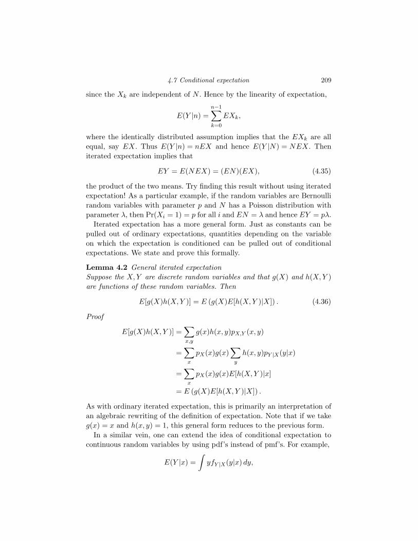
4.7 Conditional expectation 209

since the Xk are independent of N . Hence by the linearity of expectation,

E(Y |n) =n−1∑

k=0

EXk,

where the identically distributed assumption implies that the EXk are all

equal, say EX. Thus E(Y |n) = nEX and hence E(Y |N) = NEX. Then

iterated expectation implies that

EY = E(NEX) = (EN)(EX), (4.35)

the product of the two means. Try finding this result without using iterated

expectation! As a particular example, if the random variables are Bernoulli

random variables with parameter p and N has a Poisson distribution with

parameter λ, then Pr(Xi = 1) = p for all i and EN = λ and hence EY = pλ.

Iterated expectation has a more general form. Just as constants can be

pulled out of ordinary expectations, quantities depending on the variable

on which the expectation is conditioned can be pulled out of conditional

expectations. We state and prove this formally.

Lemma 4.2 General iterated expectation

Suppose the X,Y are discrete random variables and that g(X) and h(X,Y )

are functions of these random variables. Then

E[g(X)h(X,Y )] = E (g(X)E[h(X,Y )|X]) . (4.36)

Proof

E[g(X)h(X,Y )] =∑

x,y

g(x)h(x, y)pX,Y (x, y)

=∑

x

pX(x)g(x)∑

y

h(x, y)pY |X(y|x)

=∑

x

pX(x)g(x)E[h(X,Y )|x]

= E (g(X)E[h(X,Y )|X]) .

As with ordinary iterated expectation, this is primarily an interpretation of

an algebraic rewriting of the definition of expectation. Note that if we take

g(x) = x and h(x, y) = 1, this general form reduces to the previous form.

In a similar vein, one can extend the idea of conditional expectation to

continuous random variables by using pdf’s instead of pmf’s. For example,

E(Y |x) =

∫yfY |X(y|x) dy,

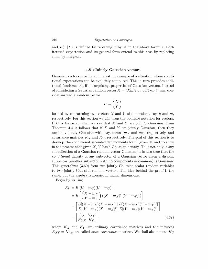
210 Expectation and averages

and E(Y |X) is defined by replacing x by X in the above formula. Both

iterated expectation and its general form extend to this case by replacing

sums by integrals.

4.8 ⋆Jointly Gaussian vectors

Gaussian vectors provide an interesting example of a situation where condi-

tional expectations can be explicitly computed. This in turn provides addi-

tional fundamental, if unsurprising, properties of Gaussian vectors. Instead

of considering a Gaussian random vector X = (X0,X1, . . . ,XN−1)t, say, con-

sider instead a random vector

U =

(X

Y

)

formed by concatening two vectors X and Y of dimensions, say, k and m,

respectively. For this section we will drop the boldface notation for vectors.

If U is Gaussian, then we say that X and Y are jointly Gaussian. From

Theorem 4.4 it follows that if X and Y are jointly Gaussian, then they

are individually Gaussian with, say, means mX and mY , respectively, and

covariance matrices KX and KY , respectively. The goal of this section is to

develop the conditional second-order moments for Y given X and to show

in the process that given X, Y has a Gaussian density. Thus not only is any

subcollection of a Gaussian random vector Gaussian, it is also true that the

conditional density of any subvector of a Gaussian vector given a disjoint

subvector (another subvector with no components in common) is Gaussian.

This generalizes (3.60) from two jointly Gaussian scalar random variables

to two jointly Gaussian random vectors. The idea behind the proof is the

same, but the algebra is messier in higher dimensions.

Begin by writing

KU = E[(U − mU )(U − mU)t]

= E

[(X − mX

Y − mY

)((X − mX)t (Y − mY )t)

]

=

[E[(X − mX)(X − mX)t] E[(X − mX)(Y − mY )t]

E[(Y − mY )(X − mX)t] E[(Y − mY )(Y − mY )t]

]

=

[KX KXY

KY X KY

], (4.37)

where KX and KY are ordinary covariance matrices and the matrices

KXY = KtY X are called cross-covariance matrices. We shall also denote KU

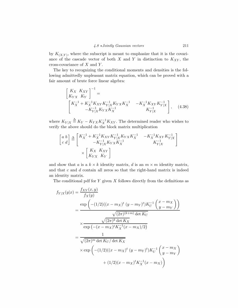
4.8 ⋆Jointly Gaussian vectors 211

by K(X,Y ), where the subscript is meant to emphasize that it is the covari-

ance of the cascade vector of both X and Y in distinction to KXY , the

cross-covariance of X and Y .

The key to recognizing the conditional moments and densities is the fol-

lowing admittedly unpleasant matrix equation, which can be proved with a

fair amount of brute force linear algebra:

[KX KXY

KY X KY

]−1

=

[K−1

X + K−1X KXY K−1

Y |XKY XK−1X −K−1

X KXY K−1Y |X

−K−1Y |XKY XK−1

X K−1Y |X

], (4.38)

where KY |X∆= KY − KY XK−1

X KXY . The determined reader who wishes to

verify the above should do the block matrix multiplication

[a b

c d

]∆=

[K−1

X + K−1X KXY K−1

Y |XKY XK−1X −K−1

X KXY K−1Y |X

−K−1Y |XKY XK−1

X K−1Y |X

]

×[

KX KXY

KY X KY

]

and show that a is a k × k identity matrix, d is an m × m identity matrix,

and that c and d contain all zeros so that the right-hand matrix is indeed

an identity matrix.

The conditional pdf for Y given X follows directly from the definitions as

fY |X(y|x) =fXY (x, y)

fX(y)

=

exp

(−(1/2)((x − mX)t (y − mY )t)K−1

U

(x − mX

y − mY

))

√(2π)(k+m) det KU

×√

(2π)k detKX

exp(−(x − mX)tK−1

X (x − mX)/2)

=1√

(2π)m detKU/det KX

× exp

(−(1/2)((x − mX)t (y − mY )t)K−1

U

(x − mX

y − mY

)

+ (1/2)(x − mX)tK−1X (x − mX)

)

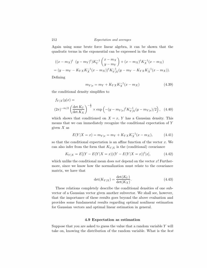
212 Expectation and averages

Again using some brute force linear algebra, it can be shown that the

quadratic terms in the exponential can be expressed in the form

((x − mX)t (y − mY )t)K−1U

(x − mX

y − mY

)+ (x − mX)tK−1

X (x − mX)

= (y − mY − KY XK−1X (x − mX))tK−1

Y |X(y − mY − KY XK−1X (x − mX)).

Defining

mY |x = mY + KY XK−1X (x − mX) (4.39)

the conditional density simplifies to

fY |X(y|x) =

(2π)−m/2

(det KU

detKX

)− 12

× exp(−(y − mY |x)tK−1

Y |X(y − mY |x)/2)

, (4.40)

which shows that conditioned on X = x, Y has a Gaussian density. This

means that we can immediately recognize the conditional expectation of Y

given X as

E(Y |X = x) = mY |x = mY + KY XK−1X (x − mX), (4.41)

so that the conditional expectation is an affine function of the vector x. We

can also infer from the form that KY |X is the (conditional) covariance

KY |X = E[(Y − E(Y |X = x))(Y − E(Y |X = x))t|x], (4.42)

which unlike the conditional mean does not depend on the vector x! Further-

more, since we know how the normalization must relate to the covariance

matrix, we have that

det(KY |X) =det(KU )

det(KX). (4.43)

These relations completely describe the conditional densities of one sub-

vector of a Gaussian vector given another subvector. We shall see, however,

that the importance of these results goes beyond the above evaluation and

provides some fundamental results regarding optimal nonlinear estimation

for Gaussian vectors and optimal linear estimation in general.

4.9 Expectation as estimation

Suppose that you are asked to guess the value that a random variable Y will

take on, knowing the distribution of the random variable. What is the best

4.9 Expectation as estimation 213

guess or estimate, say Y ? Obviously there are many ways to define a best

estimate, but one of the most popular ways to define a cost or distortion

resulting from estimating the “true” value of Y by Y is to look at the

expected value of the square of the error Y − Y , E[(Y − Y )2], the so-called

mean squared error or mean square error or simply MSE. Many arguments

have been advanced in support of this approach, perhaps the simplest being

that if one views the error as a voltage, then the average squared error is the

average energy in the error. The smaller the energy, the weaker the signal in

some sense. Perhaps a more honest reason for the popularity of the measure

is its tractability in a wide variety of problems; it often leads to nice solutions

that indeed work well in practice. As an example, we show that the optimal

estimate of the value of an unknown random variable in the minimum mean

squared error sense is in fact the mean of the random variable, a result that

is highly intuitive. Rather than use calculus to prove this result – a tedious

approach requiring setting derivatives to zero and then looking at second

derivatives to verify that the stationary point is a minimum – we directly

prove the global optimality of the result. Suppose that that our estimate is

Y is some constant a. We will show that this estimate can never have mean

squared error smaller than that resulting from using the expected value of

Y as an estimate. This is accomplished by a simple sequence of equalities

and inequalities. Begin by adding and subtracting the mean, expanding the

square, and using the second and third properties of expectation as

E[(Y − a)2] = E[(Y − EY + EY − a)2]

= E[(Y − EY )2] + 2E[(Y − EY )(EY − a)] + (EY − a)2.

The cross-product is evaluated using the linearity of expectation and the

fact that EY is a constant as

E[(Y − EY )(EY − a)] = (EY )2 − aEY − (EY )2 + aEY = 0

and hence from Property 1 of expectation,

E[(Y − a)2] = E[(Y − EY )2] + (EY − a)2 ≥ E[(Y − EY )2], (4.44)

which is the mean squared error resulting from using the mean of Y as an

estimate. Thus the mean of a random variable is the minimum mean squared

error (MMSE) estimate of the value of a random variable in the absence of

any a-priori information.

What if one is given a-priori information? For example, suppose that now

you are told that X = x. What then is the best estimate of Y , say Y (X)?

This problem is easily solved by modifying the previous derivation to use

214 Expectation and averages

conditional expectation, that is, by using the conditional distribution for

Y given X instead of the a-priori distribution for Y . Once again we try to

minimize the mean squared error:

E[(Y − Y (X))2] = E(E[(Y − Y (X))2|X]

)

=∑

x

pX(x)E[(Y − Y (X))2|x].

Each of the terms in the sum, however, is just a mean squared error between

a random variable and an estimate of that variable with respect to a distri-

bution, here the conditional distribution pY |X(·|x). By the same argument

as was used in the unconditional case, the best estimate is the mean, but

now the mean with respect to the conditional distribution, i.e., E(Y |x). In

other words, for each x the best Y (x) in the sense of minimizing the mean

squared error is E(Y |x). Plugging in the random variable X in place of the

dummy variable x we have the following interpretation:

• The conditional expectation E(Y |X) of a random variable Y given a random

variable X is the minimum mean squared estimate of Y given X .

A direct proof of this result without invoking the conditional version of the

result for unconditional expectation follows from general iterated expecta-

tion. Suppose that g(X) is an estimate of Y given X. Then the resulting

mean squared error is

E[(Y − g(X))2] = E[(Y − E(Y |X) + E(Y |X) − g(X))2]

= E[(Y − E(Y |X))2]

−2E[(Y − E(Y |X))(E(Y |X) − g(X))]

+E[(E(Y |X) − g(X))2].

Expanding the cross term yields

E[(Y − E(Y |X))(E(Y |X) − g(X))] =

E[Y E(Y |X)] − E[Y g(X)] − E[E(Y |X)2] + E[E(Y |X)g(X)].

From the general iterated expectation (4.36), E[Y E(Y |X)] = E[E(Y |X)2]

(setting g(X) of the lemma to E(Y |X) and h(X,Y ) = Y ); and E[Y g(X)] =

E[E(Y |X)g(X)] (setting g(X) of the lemma to the g(X) used here and

h(X,Y ) = Y ).

As with ordinary expectation, the ideas of conditional expectation can be

extended to continuous random variables by substituting conditional pdf’s

for the unconditional pdf’s. As is the case with conditional probability, how-

4.9 Expectation as estimation 215

ever, this constructive definition has its limitations and only makes sense

when the pdf’s are well defined. The rigorous development of conditional

expectation is, like conditional probability, analogous to the rigorous treat-

ment of the Dirac delta; it is defined by its behavior underneath the integral

sign rather than by a construction. When the constructive definition makes

sense, the two approaches agree.

The conditional expectation cannot be explicitly evaluated in most cases.

However, for the very important case of jointly Gaussian random variables

we can immediately identify from (3.60) that

E[Y |X] = mY + ρ(σY /σX)(X − mX). (4.45)

It is important that this is in fact an affine function of X.

The same ideas extend from scalars to vectors. Suppose we observe a

real-valued column vector X = (X0, . . . ,Xk−1)t and we wish to predict or

estimate a second random vector Y = (Y0, . . . , Ym−1)t. Note that the dimen-

sions of the two vectors need not be the same.

The prediction Y = Y (X) is to be chosen as a function of X which yields

the smallest possible mean squared error, as in the scalar case. The mean

squared error is defined as

ǫ2(Y ) = E(‖Y − Y ‖2)∆= E[(Y − Y )t(Y − Y )]

=

m−1∑

i=0

E[(Yi − Yi)2]. (4.46)

An estimator or predictor is said to be optimal within some class of predictors

if it minimizes the mean squared error over all predictors in the given class.

Two specific examples of vector estimation are of particular interest. In the

first case, the vector X consists of k consecutive samples from a stationary

random process, say X = (Xn−1,Xn−2, . . . ,Xn−k) and Y is the one step

ahead, next, or “future”, sample Y = Xn. In this case the goal is to find

the best one-step predictor given the finite past. In the second example, Y

is a rectangular subblock of pixels in a sampled image intensity raster and

X consists of similar subgroups above and to the left of Y . Here the goal

is to use portions of an image already coded or processed to predict a new

portion of the same image. This vector prediction problem is depicted in

Figure 4.1 where subblocks A, B, and C would be used to predict subblock

D.

The following theorem shows that the best nonlinear predictor of Y given

X is simply the conditional expectation of Y given X. Intuitively, our best

guess of an unknown vector is its expectation or mean given whatever ob-

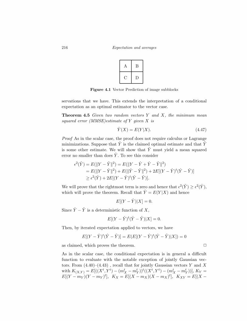
216 Expectation and averages

C

A B

D

Figure 4.1 Vector Prediction of image subblocks

servations that we have. This extends the interpretation of a conditional

expectation as an optimal estimator to the vector case.

Theorem 4.5 Given two random vectors Y and X, the minimum mean

squared error (MMSE)estimate of Y given X is

Y (X) = E(Y |X). (4.47)

Proof As in the scalar case, the proof does not require calculus or Lagrange

minimizations. Suppose that Y is the claimed optimal estimate and that Y

is some other estimate. We will show that Y must yield a mean squared

error no smaller than does Y . To see this consider

ǫ2(Y ) = E(‖Y − Y ‖2) = E(‖Y − Y + Y − Y ‖2)

= E(‖Y − Y ‖2) + E(‖Y − Y ‖2) + 2E[(Y − Y )t(Y − Y )]

≥ ǫ2(Y ) + 2E[(Y − Y )t(Y − Y )].

We will prove that the rightmost term is zero and hence that ǫ2(Y ) ≥ ǫ2(Y ),

which will prove the theorem. Recall that Y = E(Y |X) and hence

E[(Y − Y )|X] = 0.

Since Y − Y is a deterministic function of X,

E[(Y − Y )t(Y − Y )|X] = 0.

Then, by iterated expectation applied to vectors, we have

E[(Y − Y )t(Y − Y )] = E(E[(Y − Y )t(Y − Y )|X]) = 0

as claimed, which proves the theorem. 2

As in the scalar case, the conditional expectation is in general a difficult

function to evaluate with the notable exception of jointly Gaussian vec-

tors. From (4.40)–(4.43) , recall that for jointly Gaussian vectors Y and X

with K(X,Y ) = E[((Xt, Y t) − (mtX − mt

Y ))t((Xt, Y t) − (mtX − mt

Y ))], KY =

E[(Y − mY )(Y − mY )t], KX = E[(X − mX)(X − mX)t], KXY = E[(X −

4.9 Expectation as estimation 217

mX)(Y − mY )t], KY X = E[(Y − mY )(Y − mY )t] the conditional pdf is is

fY |X(y|x) = (2π)−m/2(det(KY |X))−12 ×

exp

(−

(y − mY |x)tK−1

Y |X(y − mY |x)

2

), (4.48)

where

KY |X∆= KY − KY XK−1

X KXY

= E[(Y − E(Y |X))(Y − E(Y |X))t|X], (4.49)

det(KY |X) =det(K(Y,X))

det(KX), (4.50)

and

E(Y |X = x) = mY |x = mY + KY XK−1X (x − mX), (4.51)

and hence the minimum mean squared error estimate of Y given X is

E(Y |X) = mY + KY XK−1X (X − mX) , (4.52)

which is an affine function of X! The resulting minimum mean squared error

is (using iterated expectation)

E[(Y − E(Y |X))t(Y − E(Y |X))]

= E(E[(Y − E(Y |X))t(Y − E(Y |X))|X]

)

= E(E[Tr[(Y − E(Y |X))(Y − E(Y |X))t]|X]

)

= Tr(KY |X). (4.53)

In the special case where X = Xn = (X0,X1, . . . ,Xn−1) and Y = Xn, the

so-called one-step linear prediction problem, the solution takes an interesting

form. For this case define the nth-order covariance matrix as the n × n

matrix

K(n)X = E[(Xn − E(Xn))(Xn − E(Xn))t], (4.54)

i.e., the (k, j) entry of K(n)X is E[(Xk − E(Xk))(Xj − E(Xj))], k, j =

0, 1, . . . , n − 1. Then if Xn+1 is Gaussian, the optimal one-step predictor

for Xn given Xn is

Xn(Xn) =

E(Xn) + E[(Xn − E(Xn))(Xn − E(Xn))t](K(n)X )−1(Xn − E(Xn)) (4.55)

218 Expectation and averages

which has an affine form

Xn(Xn) = AXn + b (4.56)

where

A = rt(K(n)X )−1, (4.57)

r =

KX(n, 0)

KX(n, 1)...

KX(n, n − 1)

, (4.58)

and

b = E(Xn) − AE(Xn). (4.59)

The resulting mean squared error is

MMSE = E[(Xn − Xn(Xn))2]

= Tr(KY − KY XK−1X KXY )

= σ2Xn

− rt(K(n)X )−1r

or

MMSE = E[(Xn − Xn(Xn))2] = σ2Xn|Xn , (4.60)

which from (4.50) can be expressed as

MMSE =det(K

(n)X )

det(K(n−1)X )

, (4.61)

a classical result from minimum mean squared error estimation theory.

A special case of interest occurs when the mean of Xn is constant for all

n and the covariance function has the property that

KX(k, l) = KX(k + n, l + n), all k, l, n,

that is, the covariance function evaluated at two sample times is unchanged if

both sample times are shifted by an equal amount. In this case the covariance

of two samples depends only on how far apart in time they are and not on the

actual absolute time of each. As we shall detail in Section 4.18, a process with

this property is said to be weakly stationary . In this case with the added

assumption (for simplicity) that the constant mean is zero, the estimator

4.10 ⋆Implications for linear estimation 219

simplifies to

Xn(Xn) = rt(K(n)X )−1Xn, (4.62)

where r is the n-dimensional vector

r =

KX(n)

KX(n − 1)...

KX(1)

. (4.63)

4.10 ⋆Implications for linear estimation

The development of minimum mean squared error estimation for the Gaus-

sian case provides a preview and an approach to the problem of minimum

mean squared estimation for the situation of completely general random

vectors (not necessarily Gaussian) where only linear or affine estimators are

allowed (to avoid the problem of possibly intractable conditional expecta-

tions in the non-Gaussian case). This topic will be developed in some detail

in a later section, but the key results will be shown to follow directly from

the Gaussian case by reinterpreting the results.

The key fact is that the optimal estimator for a vector Y given a vector

X when the two are jointly Gaussian was found to be an affine estimator,

that is, to have the form

Y (X) = AX + b.

The MMSE was found over all possible estimators as an estimator of this

form with A = KY XK−1X and b = E(Y ) + AE(X) with a resulting MMSE

= Tr(KY − KY XK−1X KXY ). Therefore it is obviously true that this MMSE

must be the minimum achievable MSE over all affine estimators, i.e., that

for all k × m matrices A and m-dimensional vectors b it is true that

MSE(A, b) = Tr((Y − AX − b)(Y − AX − b)t

)

≥ Tr(KY − KY XK−1X KXY ) (4.64)

and that equality holds if and only if A = KY XK−1X and b = E(Y ) + AE(X).

We shall now see that this version of the result has nothing to do with

Gaussianity and that the inequality and solution are true for any distribution

(providing of course that KX is invertible).

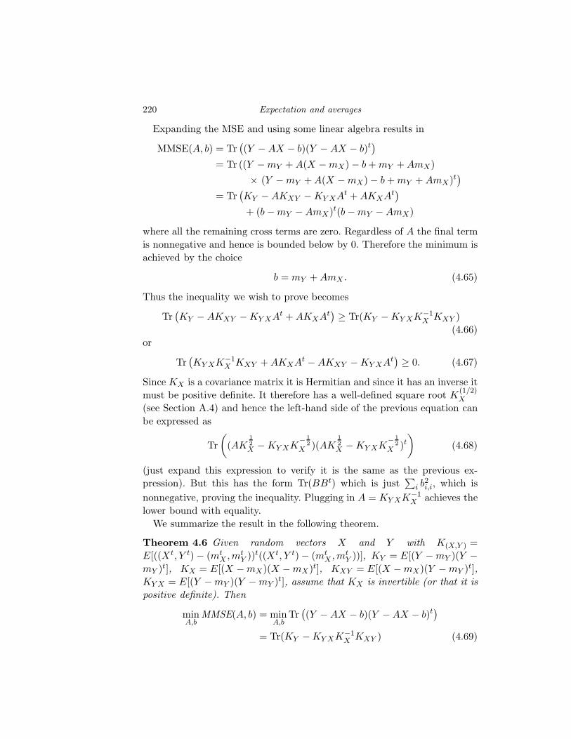
220 Expectation and averages

Expanding the MSE and using some linear algebra results in

MMSE(A, b) = Tr((Y − AX − b)(Y − AX − b)t

)

= Tr ((Y − mY + A(X − mX) − b + mY + AmX)

× (Y − mY + A(X − mX) − b + mY + AmX)t)

= Tr(KY − AKXY − KY XAt + AKXAt

)

+ (b − mY − AmX)t(b − mY − AmX)

where all the remaining cross terms are zero. Regardless of A the final term

is nonnegative and hence is bounded below by 0. Therefore the minimum is

achieved by the choice

b = mY + AmX . (4.65)

Thus the inequality we wish to prove becomes

Tr(KY − AKXY − KY XAt + AKXAt

)≥ Tr(KY − KY XK−1

X KXY )

(4.66)

or

Tr(KY XK−1

X KXY + AKXAt − AKXY − KY XAt)≥ 0. (4.67)

Since KX is a covariance matrix it is Hermitian and since it has an inverse it

must be positive definite. It therefore has a well-defined square root K(1/2)X

(see Section A.4) and hence the left-hand side of the previous equation can

be expressed as

Tr

((AK

12X − KY XK

− 12

X )(AK12X − KY XK

− 12

X )t)

(4.68)

(just expand this expression to verify it is the same as the previous ex-

pression). But this has the form Tr(BBt) which is just∑

i b2i,i, which is

nonnegative, proving the inequality. Plugging in A = KY XK−1X achieves the

lower bound with equality.

We summarize the result in the following theorem.

Theorem 4.6 Given random vectors X and Y with K(X,Y ) =

E[((Xt, Y t) − (mtX ,mt

Y ))t((Xt, Y t) − (mtX ,mt

Y ))], KY = E[(Y − mY )(Y −mY )t], KX = E[(X − mX)(X − mX)t], KXY = E[(X − mX)(Y − mY )t],

KY X = E[(Y − mY )(Y − mY )t], assume that KX is invertible (or that it is

positive definite). Then

minA,b

MMSE(A, b) = minA,b

Tr((Y − AX − b)(Y − AX − b)t

)

= Tr(KY − KY XK−1X KXY ) (4.69)

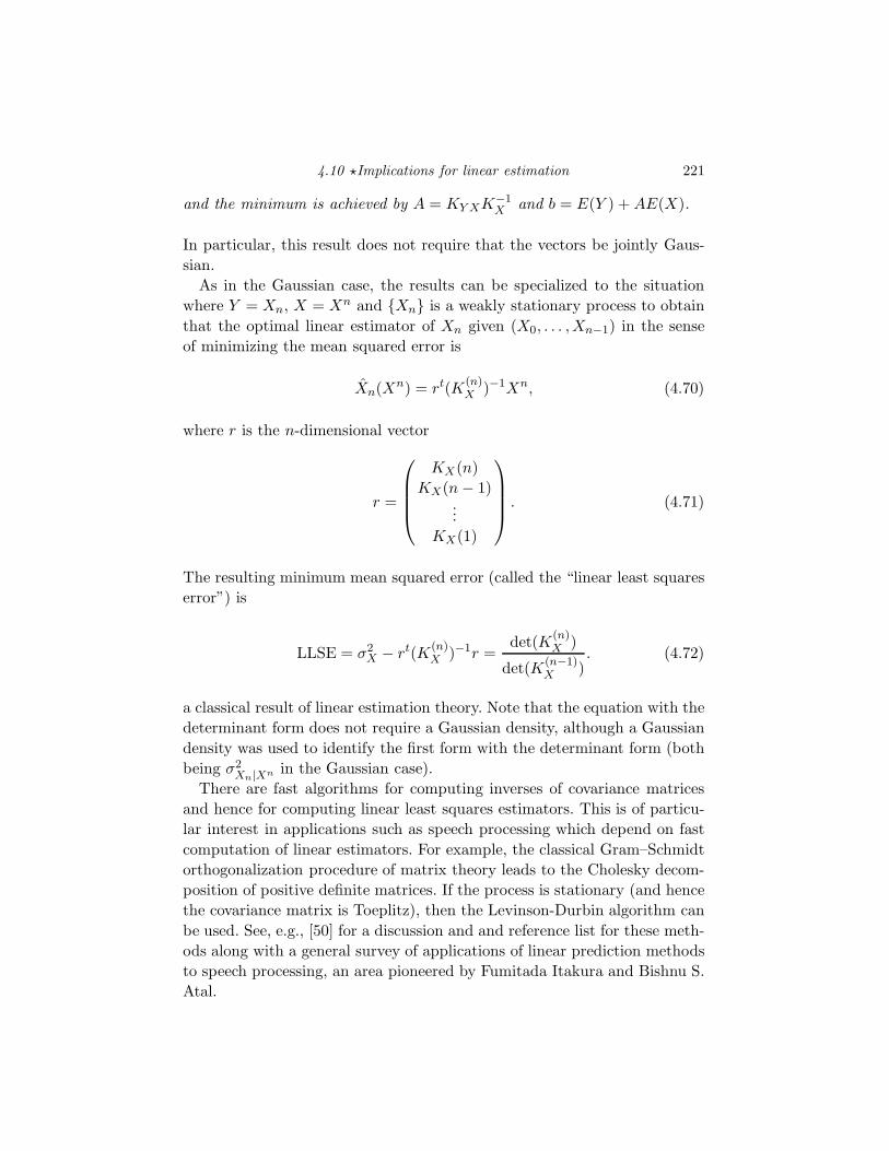
4.10 ⋆Implications for linear estimation 221

and the minimum is achieved by A = KY XK−1X and b = E(Y ) + AE(X).

In particular, this result does not require that the vectors be jointly Gaus-

sian.

As in the Gaussian case, the results can be specialized to the situation

where Y = Xn, X = Xn and Xn is a weakly stationary process to obtain

that the optimal linear estimator of Xn given (X0, . . . ,Xn−1) in the sense

of minimizing the mean squared error is

Xn(Xn) = rt(K(n)X )−1Xn, (4.70)

where r is the n-dimensional vector

r =

KX(n)

KX(n − 1)...

KX(1)

. (4.71)

The resulting minimum mean squared error (called the “linear least squares

error”) is

LLSE = σ2X − rt(K

(n)X )−1r =

det(K(n)X )

det(K(n−1)X )

. (4.72)

a classical result of linear estimation theory. Note that the equation with the

determinant form does not require a Gaussian density, although a Gaussian

density was used to identify the first form with the determinant form (both

being σ2Xn|Xn in the Gaussian case).

There are fast algorithms for computing inverses of covariance matrices

and hence for computing linear least squares estimators. This is of particu-

lar interest in applications such as speech processing which depend on fast

computation of linear estimators. For example, the classical Gram–Schmidt

orthogonalization procedure of matrix theory leads to the Cholesky decom-

position of positive definite matrices. If the process is stationary (and hence

the covariance matrix is Toeplitz), then the Levinson-Durbin algorithm can

be used. See, e.g., [50] for a discussion and and reference list for these meth-

ods along with a general survey of applications of linear prediction methods

to speech processing, an area pioneered by Fumitada Itakura and Bishnu S.

Atal.

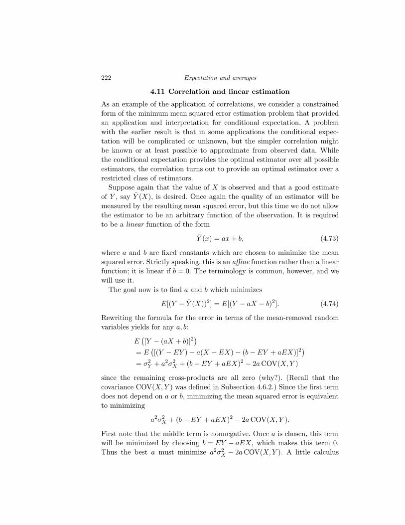
222 Expectation and averages

4.11 Correlation and linear estimation

As an example of the application of correlations, we consider a constrained

form of the minimum mean squared error estimation problem that provided

an application and interpretation for conditional expectation. A problem

with the earlier result is that in some applications the conditional expec-

tation will be complicated or unknown, but the simpler correlation might

be known or at least possible to approximate from observed data. While

the conditional expectation provides the optimal estimator over all possible

estimators, the correlation turns out to provide an optimal estimator over a

restricted class of estimators.

Suppose again that the value of X is observed and that a good estimate

of Y , say Y (X), is desired. Once again the quality of an estimator will be

measured by the resulting mean squared error, but this time we do not allow

the estimator to be an arbitrary function of the observation. It is required

to be a linear function of the form

Y (x) = ax + b, (4.73)

where a and b are fixed constants which are chosen to minimize the mean

squared error. Strictly speaking, this is an affine function rather than a linear

function; it is linear if b = 0. The terminology is common, however, and we

will use it.

The goal now is to find a and b which minimizes

E[(Y − Y (X))2] = E[(Y − aX − b)2]. (4.74)

Rewriting the formula for the error in terms of the mean-removed random

variables yields for any a, b:

E([Y − (aX + b)]2

)

= E([(Y − EY ) − a(X − EX) − (b − EY + aEX)]2

)

= σ2Y + a2σ2

X + (b − EY + aEX)2 − 2aCOV(X,Y )

since the remaining cross-products are all zero (why?). (Recall that the

covariance COV(X,Y ) was defined in Subsection 4.6.2.) Since the first term

does not depend on a or b, minimizing the mean squared error is equivalent

to minimizing

a2σ2X + (b − EY + aEX)2 − 2aCOV(X,Y ).

First note that the middle term is nonnegative. Once a is chosen, this term

will be minimized by choosing b = EY − aEX, which makes this term 0.

Thus the best a must minimize a2σ2X − 2aCOV(X,Y ). A little calculus

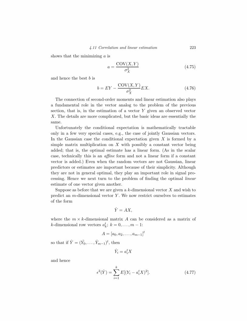
4.11 Correlation and linear estimation 223

shows that the minimizing a is

a =COV(X,Y )

σ2X

(4.75)

and hence the best b is

b = EY − COV(X,Y )

σ2X

EX. (4.76)

The connection of second-order moments and linear estimation also plays

a fundamental role in the vector analog to the problem of the previous

section, that is, in the estimation of a vector Y given an observed vector

X. The details are more complicated, but the basic ideas are essentially the

same.

Unfortunately the conditional expectation is mathematically tractable

only in a few very special cases, e.g., the case of jointly Gaussian vectors.

In the Gaussian case the conditional expectation given X is formed by a

simple matrix multiplication on X with possibly a constant vector being

added; that is, the optimal estimate has a linear form. (As in the scalar

case, technically this is an affine form and not a linear form if a constant

vector is added.) Even when the random vectors are not Gaussian, linear

predictors or estimates are important because of their simplicity. Although

they are not in general optimal, they play an important role in signal pro-

cessing. Hence we next turn to the problem of finding the optimal linear

estimate of one vector given another.

Suppose as before that we are given a k-dimensional vector X and wish to

predict an m-dimensional vector Y . We now restrict ourselves to estimates

of the form

Y = AX,

where the m × k-dimensional matrix A can be considered as a matrix of

k-dimensional row vectors atk; k = 0, . . . ,m − 1:

A = [a0, a2, . . . , am−1]t

so that if Y = (Y0, . . . , Ym−1)t, then

Yi = atiX

and hence

ǫ2(Y ) =k∑

i=1

E[(Yi − atiX)2]. (4.77)

224 Expectation and averages

The goal is to find the matrix A that minimizes ǫ2. This can be considered

as a function of the estimate Y or of the matrix A defining the estimate.

We shall provide two separate solutions which are almost, but not quite,

equivalent. The first is constructive in nature: a specific A will be given and

shown to be optimal. The second development is descriptive: without actu-

ally giving the matrix A, we will show that a certain property is necessary

and sufficient for the matrix to be optimal. That property is called the or-

thogonality principle. It states that the optimal matrix is the one that causes

the error vector Y − Y to be orthogonal to (have zero correlation with) the

observed vector X. The first development is easier to use because it pro-

vides a formula for A that can be immediately computed in many cases.

The second development is less direct and less immediately applicable, but

it turns out to be more general: the descriptive property can be used to de-

rive A even when the first development is not applicable. The orthogonality

principle plays a fundamental role in all of linear estimation theory.

The error ǫ2(A) is minimized if each term E[(Yi − atiX)2] is minimized

over ai since there is no interaction among the terms in the sum. We can do

no better when minimizing a sum of such positive terms than to minimize

each term separately. Thus the fundamental problem is the following simpler

one: given a random vector X and a random variable (one-dimensional or

scalar vector) Y , we seek a vector a that minimizes

ǫ2(a) = E[(Y − atX)2]. (4.78)

One way to find the optimal a is to use calculus, setting derivatives of

ǫ2(a) to zero and verifying that the stationary point so obtained is a global

minimum. As previously discussed, variational techniques can be avoided

via elementary inequalities if the answer is known. We shall show that the

optimal a is a solution of

atRX = E(Y Xt), (4.79)

so that if the autocorrelation matrix defined by

RX = E[XXt] = RX(k, i) = E(XkXi); k, i = 0, . . . , k − 1

is invertible, then the optimal a is given by

at = E(Y Xt)R−1X . (4.80)

To prove this we assume that a satisfies (4.80) and show that for any other

vector b

ǫ2(b) ≥ ǫ2(a) . (4.81)

4.11 Correlation and linear estimation 225

To do this we write

ǫ2(b) = E[(Y − btX)2] = E[(Y − atX + atX − btX)2]

= E[(Y − atX)2] + 2E[(Y − atX)(atX − btX)] + E[(atX − btX)2].

Of the final terms, the first term is just ǫ2(a) and the rightmost term is

obviously nonnegative. Thus we have the bound

ǫ2(b) ≥ ǫ2(a) + 2E[(Y − atX)(at − bt)X]. (4.82)

The cross-product term can be written as

2E[(Y − atX)(at − bt)X] = 2E[(Y − atX)Xt(a − b)]

= 2E[(Y − atX)Xt](a − b)

= 2(E[Y Xt] − atE[XXt]

)(a − b)

= 2(E[Y Xt] − atRX

)(a − b)

= 0 (4.83)

invoking (4.79). Combining this with (4.82) proves (4.81) and hence opti-

mality. Note that because of the symmetry of autocorrelation matrices and

their inverses, we can rewrite (4.80) as

a = (E(Y Xt)R−1X )t = R−1

X E[Y X]. (4.84)

Using the above result to perform a termwise minimization of (4.77) now

yields the following theorem describing the optimal linear vector predictor.

Theorem 4.7 The minimum mean squared error linear predictor of the

form Y = AX is given by any solution A of the equation

ARX = E(Y Xt).

If the matrix RX is invertible, then A is uniquely given by

At = R−1X E[XY t] ,

that is, the matrix A has rows ati; i = 0, 1, . . . ,m, with

ai = R−1X E[YiX].

Alternatively,

A = E[Y Xt]R−1X . (4.85)

Having found the best linear estimate, it is easy to modify the development

to find the best estimate of the form

Y (X) = AX + b, (4.86)

226 Expectation and averages

where now we allow an additional constant term. This is also often called a

linear estimate, although as previously noted it is more correctly called an

affine estimate because of the extra constant vector term. As the end result

and proof strongly resemble the linear estimate result, we proceed directly

to the theorem.

Theorem 4.8 The minimum mean squared estimate of the form Y = AX +

b is given by any solution A of the equation

AKX = E[(Y − E(Y ))(X − E(X))t] , (4.87)

where the covariance matrix KX is defined by

KX = E[(X − E(X))(X − E(X))t] = RX−E(X),

and

b = E(Y ) − AE(X).

If KX is invertible, then

A = E[(Y − E(Y ))(X − E(X))t]K−1X . (4.88)

Note that if X and Y have zero-means, then the result reduces to the

previous result; that is, affine predictors offer no advantage over linear pre-

dictors for zero-mean random vectors.

Proof Let C be any matrix and d any vector (both of suitable dimensions)

and note that

E(‖Y − (CX + d)‖2)

= E(‖(Y − E(Y )) − C(X − E(X)) + E(Y ) − CE(X) − d‖2)

= E(‖(Y − E(Y )) − C(X − E(X))‖2) + E(‖E(Y ) − CE(X) − d‖2)

+ 2E[Y − E(Y ) − C(X − E(X))]t[E(Y ) − CE(X) − d].

From Theorem 4.7, the first term is minimized by choosing C = A, where

A is a solution of (4.87); also, the second term is the expectation of the

squared norm of a vector that is identically zero if C = A and d = b, and

similarly for this choice of C and d the third term is zero. Thus

E(‖Y − (CX + d)‖2) ≥ E(‖Y − (AX + b)‖2).

We often restrict interest to linear estimates by assuming that the various

vectors have zero-mean. This is not always possible, however. For example,

groups of pixels in a sampled image intensity raster can be used to predict

other pixel groups, but pixel values are always nonnegative and hence have

4.11 Correlation and linear estimation 227

nonzero-means. Hence in some problems affine predictors may be preferable.

Nonetheless, we will often follow the common practice of focusing on the

linear case and extending when necessary. In most studies of linear prediction

it is assumed that the mean is zero, i.e., that any dc value of the process

has been removed. If this assumption is not made, linear estimation theory

is still applicable but will generally give inferior performance to the use of

affine prediction.

4.11.1 The orthogonality principle

Although we have proved the form of the optimal linear predictor of one

vector given another, there is another way to describe the result that is often

useful for deriving optimal linear predictors in somewhat different situations.

To develop this alternative viewpoint we focus on the error vector

e = Y − Y . (4.89)

Rewriting (4.89) as Y = Y + e points out that the vector Y can be consid-

ered as its estimate plus an error or “noise” term. The goal of an optimal

predictor is then to minimize the error energy ete =∑k−1

n=0 e2n. If the estimate

is linear, then

e = Y − AX.

As with the basic development for the linear predictor, we simplify things

for the moment. We look at the scalar prediction problem of predicting

a random variable Y by Y = atX yielding a scalar error of e = Y − Y =

Y − atX. Since we have seen that the overall mean squared error E[ete]

in the vector case is minimized by separately minimizing each component

E[e2k], we can later easily extend our results for the scalar case to the vector

case.

Suppose that a is chosen optimally and consider the crosscorrelation be-

tween an arbitrary error term and the observable vector:

E[(Y − Y )X] = E[(Y − atX)X]

= E[Y X] − E[X(Xta)]

= E[Y X] − RXa = 0

using (4.79).

Thus for the optimal predictor, the error satisfies

E[eX] = 0,

228 Expectation and averages

or, equivalently,

E[eXn] = 0; n = 0, . . . , k. (4.90)

When two random variables e and X are such that their expected product

E(eX) is 0, they are said to be orthogonal and we write

e ⊥ X.

We have therefore shown that the optimal linear estimate of a scalar random

variable given a vector of observations causes the error to be orthogonal to

all of the observables and hence orthogonality of error and observations is a

necessary condition for optimality of a linear estimate.

Conversely, suppose that we know a linear estimate a is such that it ren-

ders the prediction error orthogonal to all of the observations. Arguing as we

have before, suppose that b is any other linear predictor vector and observe

that

ǫ2(b) = E[(Y − btX)2]

= E[(Y − atX + atX − btX)2]

≥ ǫ2(a) + 2E[(Y − atX)(atX − btX)],

where the equality holds if b = a. Letting e = Y − atX denote the error

resulting from an a that makes the error orthogonal with the observations,

the rightmost term can be rewritten as

2E[e(atX − btX)] = 2(at − bt)E[eX] = 0.

Thus we have shown that ǫ2(b) ≥ ǫ2(a) and hence no linear estimate can

outperform one yielding an error orthogonal to the observations and hence

such orthogonality is sufficient as well as necessary for optimality.

Since the optimal estimate of a vector Y given X is given by the com-

ponentwise optimal predictions given X, we have thus proved the following

alternative to Theorem 4.7.

Theorem 4.9 The orthogonality principle

A linear estimate Y = AX is optimal (in the mean squared error sense) if

and only if the resulting errors are orthogonal to the observations, that is, if

e = Y − AX, then

E[ekXn] = 0; k = 1, . . . ,K; n = 1, . . . , N.

4.12 Correlation and covariance functions 229

4.12 Correlation and covariance functions

We turn now to correlation in the framework of random processes. The

notion of an iid random process can be generalized by specifying the com-

ponent random variables to be merely uncorrelated rather than independent.

Although requiring the random process to be uncorrelated is a much weaker

requirement, the specification is sufficient for many applications, as will be

seen in several ways. In particular, in this chapter, the basic laws of large

numbers require only the weaker assumption and hence are more general

than they would be if independence were required. To define the class of

uncorrelated processes, it is convenient to introduce the notions of autocor-

relation functions and covariance functions of random processes.

Given a random process Xt; t ∈ T , the autocorrelation function

RX(t, s); t, s ∈ T is defined by

RX(t, s) = E(XtXs); all t, s ∈ T .

If the process is complex-valued instead of real-valued, the definition be-

comes

RX(t, s) = E(XtX∗s ); all t, s ∈ T .

The autocovariance function or simply the covariance function KX(t, s);

t, s,∈ T is defined by

KX(t, s) = COV(Xt,Xs).

Observe that (4.18) relates the two functions by

KX(t, s) = RX(t, s) − (EXt)(EX∗s ). (4.91)

Thus the autocorrelation and covariance functions are equal if the process

has zero-mean, that is, if EXt = 0 for all t. The covariance function of a

process Xt can be viewed as the autocorrelation function of the process

Xt − EXt formed by removing the mean from the given process to form

a new process having zero-mean.

The autocorrelation function of a random process is given by the correla-

tion of all possible pairs of samples; the covariance function is the covariance

of all possible pairs of samples. Both functions provide a measure of how de-

pendent the samples are and will be seen to play a crucial role in laws of

large numbers. Note that both definitions are valid for random processes in

either discrete time or continuous time and having either a discrete alphabet

or a continuous alphabet.

In terms of the correlation function, a random process Xt; t ∈ T is said

230 Expectation and averages

to be uncorrelated if

RX(t, s) =

E(X2

t ) if t = s

EXtEXs if t 6= s

or, equivalently, if

KX(t, s) =

σ2

Xtif t = s

0 if t 6= s.

The reader should not overlook the obvious fact that if a process is iid

or uncorrelated, the random variables are independent or uncorrelated only

if taken at different times. That is, Xt and Xs will not be independent or

uncorrelated when t = s, only when t 6= s (except, of course, in such trivial

cases as that where Xt = at, a sequence of constants where E(XtXt) =

atat = EXtEXt and hence Xt is uncorrelated with itself).

Gaussian Processes Revisited

Recall from Chapter 3 that a Gaussian random process Xt; t ∈ T is

completely described by a mean function mt; t ∈ T and a covariance func-

tion Λ(t, s); t, s ∈ T . As one might suspect, the names of these functions

come from the fact that they are indeed the mean and covariance functions

as defined in terms of expectations, i.e.,

mt = EXt (4.92)

Λ(t, s) = KX(t, s). (4.93)

The result for the mean follows immediately from our computation of the

mean of a Gaussian N(m,σ2) random variable. The result for the covariance

can be derived by brute force integration (not too bad if the integrator is well

versed in matrix transformations of multidimensional integrals) or looked up

in tables somewhere. The computation is tedious and we will simply state

the result without proof. The multidimensional characteristic functions to

be introduced later can be used to get a relatively simple proof, but again

it is not worth the effort to fill in the details.

A more important issue is the properties that were required for a co-

variance function when the Gaussian process was defined. Recall that it

was required that the covariance function of the process be symmetric, i.e.,

KX(t, s) = KX(s, t), and positive definite, i.e., given any positive integer

k, any collection of sample times t0, . . . , tk−1, and any k real numbers

4.12 Correlation and covariance functions 231

ai; i = 0, . . . , k − 1 (not all 0), then

n−1∑

i=0

n−1∑

l=0

aialKX(ti, tl) ≥ 0. (4.94)

If the process is complex-valued, then the covariance function is Hermitian,

i.e., KX(t, s) = K∗X(s, t) We now return to these conditions to see if they are

indeed necessary conditions for all covariance functions, Gaussian or not.

Symmetry is easy. It immediately follows from the definitions that

KX(t, s) = E[(Xt − EXt)(Xs − EXs)]

= E[(Xs − EXs)(Xt − EXt)]

= KX(s, t) (4.95)

and hence clearly all covariance functions of real-valued random processes

are symmetric, and so are covariance matrices formed by sampling covari-

ance functions. The Hermitian property for complex-valued random pro-

cesses follows similarly. To see that positive definiteness is indeed almost a

requirement, consider the fact that

n−1∑

i=0

n−1∑

l=0

aialKX(ti, tl) =n−1∑

i=0

n−1∑

l=0

aialE[(Xti − EXti)(Xtl − EXtl)]

= E

(n−1∑

i=0

n−1∑

l=0

aial(Xti − EXti)(Xtl − EXtl)

)

= E

∣∣∣∣∣

n−1∑

i=0

ai(Xti − EXti)

∣∣∣∣∣

2

≥ 0. (4.96)

Thus any covariance function KX must at least be nonnegative definite,

which implies that any covariance matrix formed by sampling the covariance

function must also be nonnegative definite. Thus nonnegative definiteness

is necessary for a covariance function and our requirement for a Gaussian

process was only slightly stronger than was needed. We will later see how to

define a Gaussian process when the covariance function is only nonnegative

definite and not necessarily positive definite.

A slight variation on the above argument shows that for any random vec-

tor X = (X0, . . . ,Xk−1)t, then the covariance matrix Λ = λi,l; i, l ∈ Zk

defined by λi,l = E[(Xi − EXi)(Xl − EXl)] must also be symmetric and

nonnegative definite. This was the reason for assuming that the covariance

matrix for a Gaussian random vector had at least these properties.

We make two important observations before proceeding. First, remember

232 Expectation and averages

that the four basic properties of expectation have nothing to do with inde-

pendence. In particular, whether or not the random variables involved are

independent or uncorrelated, one can always interchange the expectation op-

eration and the summation operation (Property 3), because expectation is

linear. On the other hand, one cannot interchange the expectation operation

with the product operation (this is not a property of expectation) unless the

random variables involved are uncorrelated, e.g., when they are independent.

Second, an iid process is also a discrete time uncorrelated random process

with identical marginal distributions. The converse statement is not true in

general; that is, the notion of an uncorrelated process is more general than

that of an iid process. Correlation measures only a weak pairwise degree

of independence. A random process can even be pairwise independent (and

hence uncorrelated) but still not be iid (Problem 4.31).

4.13 ⋆The central limit theorem

The characteristic function of a sum of iid Gaussian random variables has

been shown to be Gaussian, and linear combinations of jointly Gaussian

variables have also been shown to be Gaussian. Far more surprising is that

the characteristic function of the sum of many non-Gaussian random vari-

ables turns out to be approximately Gaussian if the variables are suitably

scaled and shifted. This result is called the central limit theorem and is one

of the primary reasons for the importance of Gaussian distributions. When

a large number of effects are added up with suitable scaling and shifting, the

resulting random variable looks Gaussian even if the underlying individual

effects are not at all Gaussian. This result is developed in this subsection.

Just as with laws of large numbers, there is no single central limit theorem

– there are many versions. The various central limit theorems differ in the

conditions of applicability. However, they have a common conclusion: the

distribution or characteristic function of the sum of a collection of random

variables converges to that of a Gaussian random variable. We will present

only the simplest form of central limit theorem, that for iid random variables.

Suppose that Xn is an iid random process with a common distribution

FX described by a pmf or pdf except that it has a finite mean EXn = m

and finite variance σ2Xn

= σ2. It will also be assumed that the characteristic

function MX(ju) is well behaved for small u in a manner to be made precise.

Consider the “standardized” or “normalized” sum

Rn =1

n1/2

n−1∑

i=0

Xi − m

σ. (4.97)

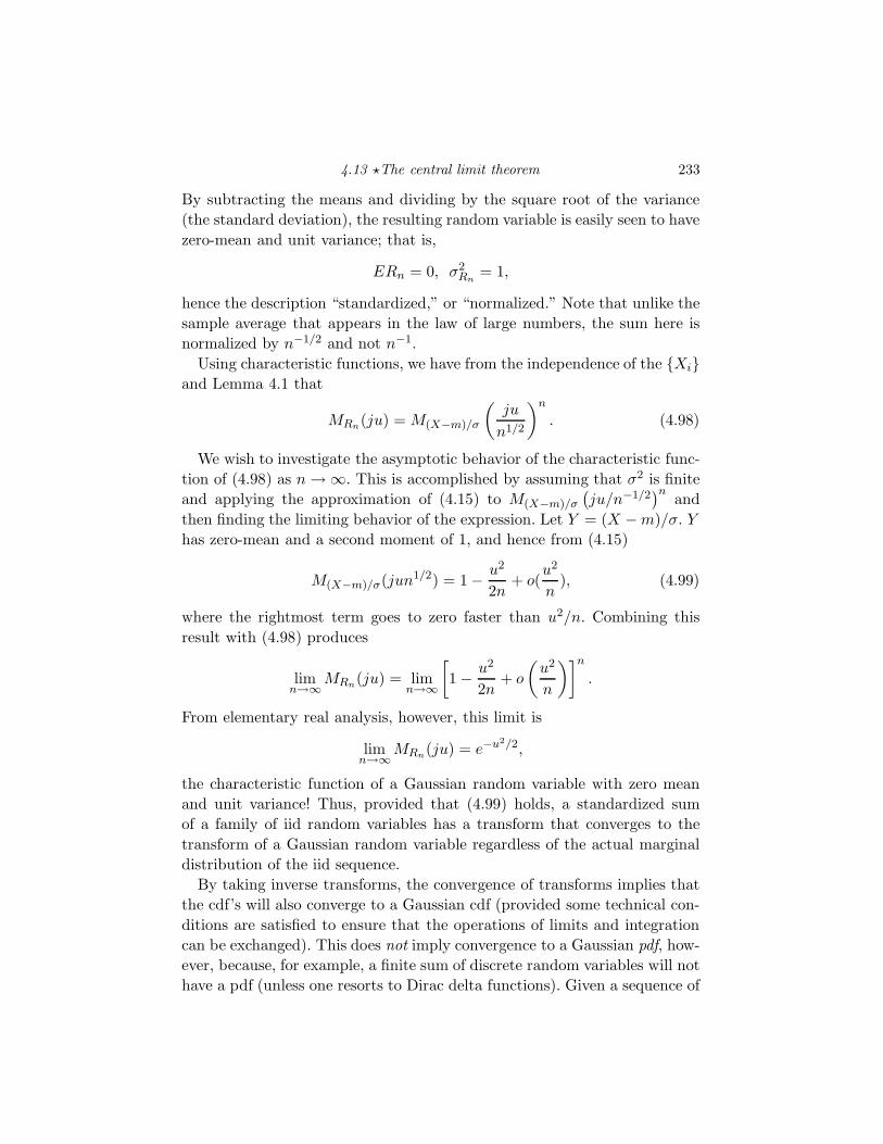
4.13 ⋆The central limit theorem 233

By subtracting the means and dividing by the square root of the variance

(the standard deviation), the resulting random variable is easily seen to have

zero-mean and unit variance; that is,

ERn = 0, σ2Rn

= 1,

hence the description “standardized,” or “normalized.” Note that unlike the

sample average that appears in the law of large numbers, the sum here is

normalized by n−1/2 and not n−1.

Using characteristic functions, we have from the independence of the Xiand Lemma 4.1 that

MRn(ju) = M(X−m)/σ

(ju

n1/2

)n

. (4.98)

We wish to investigate the asymptotic behavior of the characteristic func-

tion of (4.98) as n → ∞. This is accomplished by assuming that σ2 is finite

and applying the approximation of (4.15) to M(X−m)/σ

(ju/n−1/2

)nand

then finding the limiting behavior of the expression. Let Y = (X − m)/σ. Y

has zero-mean and a second moment of 1, and hence from (4.15)

M(X−m)/σ(jun1/2) = 1 − u2

2n+ o(

u2

n), (4.99)

where the rightmost term goes to zero faster than u2/n. Combining this

result with (4.98) produces

limn→∞

MRn(ju) = limn→∞

[1 − u2

2n+ o

(u2

n

)]n

.

From elementary real analysis, however, this limit is

limn→∞

MRn(ju) = e−u2/2,

the characteristic function of a Gaussian random variable with zero mean

and unit variance! Thus, provided that (4.99) holds, a standardized sum

of a family of iid random variables has a transform that converges to the

transform of a Gaussian random variable regardless of the actual marginal

distribution of the iid sequence.

By taking inverse transforms, the convergence of transforms implies that

the cdf’s will also converge to a Gaussian cdf (provided some technical con-

ditions are satisfied to ensure that the operations of limits and integration

can be exchanged). This does not imply convergence to a Gaussian pdf, how-

ever, because, for example, a finite sum of discrete random variables will not

have a pdf (unless one resorts to Dirac delta functions). Given a sequence of

234 Expectation and averages

random variables Rn with cdf Fn and a random variable R with distribution

F , then if limn→∞ Fn(r) = F (r) for all points r at which F (r) is continu-

ous, we say that Rn converges to R in distribution. Thus the central limit

theorem states that under certain conditions, sums of iid random variables

adjusted to have zero-mean and unit variance converge in distribution to a

Gaussian random variable with the same mean and variance.

A slight modification of the above development shows that if Xn is an

iid sequence with mean m and variance σ2, then

n−1/2n−1∑

k=0

(Xi − m)

will have a transform and a cdf converging to those of a Gaussian random

variable with mean 0 and variance σ2. We summarize the central limit the-

orem that we have established as follows.

Theorem 4.10 A central limit theorem

Let Xn be an iid random process with a finite mean m and variance σ2.

Then

n−1/2n−1∑

k=0

(Xi − m)

converges in distribution to a Gaussian random variable with mean m and

variance σ2.

Intuitively the theorem states that if we sum up a large number of indepen-

dent random variables and normalize by n−1/2 so that the variance of the

normalized sum stays constant, then the resulting sum will be approximately

Gaussian. For example, a current meter across a resistor will measure the ef-

fects of the sum of millions of electrons randomly moving and colliding with

each other. Regardless of the probabilistic description of these micro-events,

the global current will appear to be Gaussian. Making this precise yields a

model of thermal noise in resistors. Similarly, if dust particles are suspended

on a dish of water and subjected to the random collisions of millions of

molecules, then the motion of any individual particle in two dimensions will

appear to be Gaussian. Making this rigorous yields the classic model for

what is called “Brownian motion.” A similar development in one dimension

yields the Wiener process.

Note that in (4.98), if the Gaussian characteristic function is substituted

on the right-hand side, a Gaussian characteristic function appears on the

left. Thus the central limit theorem says that if you sum up random vari-

4.14 Sample averages 235

ables, you approach a Gaussian distribution. Once you have a Gaussian

distribution, you “get stuck” there – adding more random variables of the

same type (or Gaussian random variables) to the sum does not change the

Gaussian characteristic. The Gaussian distribution is an example of an in-

finitely divisible distribution – the nth root of its characteristic function is

a distribution of the same type as seen in (4.98). Equivalently stated, the

distribution class is invariant under summations.

4.14 Sample averages

In many applications, engineers analyze the average behavior of systems

based on observed data. It is important to estimate the accuracy of such

estimates as a function of the amount of data available. This and the next

sections are a prelude to such analyses. They also provide some very good

practice in manipulating expectations and a few results of interest in their

own right.

In this section we study the behavior of the arithmetic average of the

first n values of a discrete time random process with either a discrete or a

continuous alphabet. Specifically, the variance of the average is considered

as a function of n.

Suppose we are given a process Xn. The sample average of the first n

values of Xn is Sn = n−1∑n−1

i=0 Xi. The mean of Sn is found easily using

the linearity of expectation (expectation Property 3) as

ESn = E

[n−1

n−1∑

i=0

Xi

]= n−1

n−1∑

i=0

EXi. (4.100)

Hence the mean of the sample average is the same as the average of the

mean of the random variables produced by the process. Suppose now that

we assume that the mean of the random variables is a constant, EXi = X

independent of i. Then ESn = X. In terms of estimation theory, if one es-

timates an unknown random process mean, X, by Sn, then the estimate is

said to be unbiased because the expected value of the estimate is equal to

the value being estimated. Obviously an unbiased estimate is not unique,

so being unbiased is only one desirable characteristic of an estimate (Prob-

lem 4.28).

236 Expectation and averages

Next consider the variance of the sample average:

σ2Sn

∆= E[(Sn − E(Sn))2]

= E

(

n−1n−1∑

i=0

Xi − n−1n−1∑

i=0

EXi

)2

= E

(

n−1n−1∑

i=0

(Xi − EXi)

)2

= n−2n−1∑

i=0

n−1∑

j=0

E[(Xi − EXi)(Xj − EXj)].

The reader should be certain that the preceding operations are well under-

stood, as they are frequently encountered in analyses. Note that expanding

the square requires the use of separate dummy indices in order to get all

of the cross-products. Once expanded, linearity of expectation permits the

interchange of expectation and summation.

Recognizing the expectation in the sum as the covariance function, the

variance of the sample average becomes

σ2Sn

= n−2n−1∑

i=0

n−1∑

j=0

KX(i, j). (4.101)

Note that so far we have used none of the specific knowledge of the process,

i.e., the above formula holds for general discrete time processes and does not

require such assumptions as time-constant mean, time-constant variance,

identical marginal distributions, independence, uncorrelated processes, etc.

If we now use the assumption that the process is uncorrelated, the covariance

becomes zero except when i = j, and expression (4.101) becomes

σ2Sn

= n−2n−1∑

i=0

σ2Xi

. (4.102)

If we now also assume that the variances σ2Xi

are equal to some constant

value σ2X for all times i, e.g., the process has identical marginal distributions

as for an iid process, then the equations become

σ2Sn

= n−1σ2X . (4.103)

Thus, for uncorrelated discrete time random processes with mean and

variance not depending on time, the sample average has expectation equal

to the (time-constant) mean of the process, and the variance of the sample

4.15 Convergence of random variables 237

average tends to zero as n → ∞. Of course we have only specified suffi-

cient conditions. Expression (4.101) goes to zero with n under more general

circumstances, as we shall see in detail later.

For now, however, we stick with uncorrelated process with mean and vari-

ance independent of time and require only a definition to obtain our first

law of large numbers, a result implicit in equation (4.103).

4.15 Convergence of random variables

The preceding section demonstrated a form of convergence for the sequence

of random variables, Sn, the sequence of sample averages, that is different

from convergence as it is seen for a nonrandom sequence. To review, a non-

random sequence xn is said to converge to the limit x if for every ǫ > 0

there exists an N such that |xn − x| < ǫ for every n > N . The preceding

section did not see Sn converge in this sense. Nothing was said about the

individual realizations Sn(ω) as a function of ω. Only the variance of the

sequence σ2Sn

was shown to converge to zero in the usual ǫ, N sense. The

variance calculation probabilistically averages across ω. For any particular

ω, the realization Sn may, in fact, not converge to zero. It is important that

the reader understand this distinction clearly.

Thus, in order to make precise the notion of convergence of sample av-

erages to a limit, we need to make precise the notion of convergence of a

sequence of random variables. We have already seen one example of con-

vergence of random variables, the convergence in distribution used in the

central limit theorem. In this section we will describe four additional notions

of convergence of random variables. These are perhaps the most commonly

encountered, but they are by no means an exhaustive list. The common goal

is to quantify a useful definition for saying that a sequence of random vari-

ables, say Yn, n = 1, 2, . . . , converges to a random variable Y , which will be

considered the limit of the sequence. Our main application will be the case

where Yn = Sn, a sample average of n samples of a random process, and

Y is the expectation of the samples, that is, the limit is a trivial random

variable, a constant.

One might wonder why five different notions of convergence of random

variables are considered. Unfortunately no single definition is useful in all

applications and the definitions that are arguably most natural are the most

difficult to work with. Each has its uses, as will be seen.

The most straightforward generalization of the usual idea of a limit to

random variables is easy to define, but virtually useless. If for every sample

238 Expectation and averages

point ω we had limn→∞ Yn(ω) = Y (ω) in the usual sense of convergence of

numbers, then we could say that Yn converges pointwise to Y , that is, for

every sample point in the sample space. Unfortunately it is rarely possible

to prove so strong a result, nor is it necessary, nor is it usually true.

A slight variation of this yields a far more important important notion

of convergence. A sequence of random variables Yn, n = 1, 2, . . . , is said to

converge to a random variable Y with probability one or converge w.p. 1 if

the set of sample points ω such that limn→∞ Yn(ω) = Y (ω) is an event with

probability one. Thus a sequence converges with probability one if it con-

verges pointwise on a set of probability one; it can do anything outside that

set, e.g., converge to something else or not converge at all. Since the total

probability of all such bad sequences is 0, this has no practical significance.

Although convergence w.p. 1 is the easiest useful concept of convergence to

define, it is the most difficult to use. Most proofs involving convergence with

probability one are beyond the mathematical prerequisites and capabilities

of this book. Hence we will focus on two other notions of convergence that

are perhaps less intuitive to understand, but are far easier to use when prov-

ing results. First note, however, that there are many equivalent names for

convergence with probability one. It is often called convergence almost surely

and abbreviated a.s. or convergence almost everywhere and abbreviated a.e.

Convergence with probability one will not be considered in any depth here,

but some toy examples will be considered in the problems to help get the

concept across and a special case of the strong law of large numbers will be

proved in an optional section.

Henceforth two definitions of convergence for random variables will be

emphasized, both well suited to the type of results developed here (and one

that was used in historically the first such results, Bernoulli’s weak law of

large numbers for iid random processes). The first is convergence in mean

square, convergence of the type seen in the last section, which leads to a

result called a mean ergodic theorem. The second is called convergence in

probability, which is implied by the first and leads to a result called the weak

law of large numbers. The second result will follow from the first via a simple

but powerful inequality relating probabilities and expectations.

A sequence of random variables Yn; n = 1, 2, . . . is said to converge in

mean square or converge in quadratic mean to a random variable Y if

E[|Yn|2] < ∞ all n and

limn→∞

E[|Yn − Y |2] = 0.

This is also written Yn → Y in mean square or Yn → Y in quadratic mean

4.15 Convergence of random variables 239

or by

l.i.m.n→∞

Yn = Y,

where l.i.m. is an acronym for “limit in the mean.” Although it is probably

not obvious to the novice, it is important to understand that convergence

in mean square does not imply convergence with probability one. Examples

converging in one sense and not the other may be found in Problem 4.36.

Thus a sequence of random variables converges in mean square to another

random variable if the second absolute moment of the difference converges

to zero in the ordinary sense of convergence of a sequence of real numbers.

This can be given the physical interpretation that the energy in the error

goes to zero in the limit. Although the definition encompasses convergence

to a random variable with any degree of “randomness,” in most applications

that we shall encounter the limiting random variable is a degenerate random

variable, i.e., a constant. In particular, the sequence of sample averages,

Sn, of the preceding section is next seen to converge in this sense.

The final notion of convergence bears a strong resemblance to the notion

of convergence with probability one, but the resemblance is a faux ami, the

two notions are fundamentally different. A sequence of random variables

Yn; n = 1, 2, . . . is said to converge in probability to a random variable Y if

for every ǫ > 0,

limn→∞

Pr(|Yn − Y | > ǫ) = 0.

Thus a sequence of random variables converges in probability if the probabil-

ity that the nth member of the sequence differs from the limit by more than

an arbitrarily small ǫ goes to zero as n → ∞. Note that just as with conver-

gence in mean square, convergence in probability is silent on the question of

convergence of individual realizations Yn(ω). You could, in fact, have no re-

alizations converge individually and yet have convergence in probability. All

that convergence in probability tells you is that Pr(ω : |Yn(ω) − Y (ω)| > ǫ)

tends to zero with n. Suppose at time n a given subset of Ω satisfies the in-

equality, at time n + 2 still a different subset satisfies the inequality, etc. As

long as the subsets have diminishing probability, convergence in probability

can occur without convergence of the individual sequences.

Also, as in convergence in the mean square sense, convergence in proba-

bility is to a random variable in general. This includes the most interesting

case of a degenerate random variable – a constant.

The two notions of convergence – convergence in mean square and conver-

gence in probability – can be related to each other via simple, but important,

240 Expectation and averages

inequalities. It will be seen that convergence in mean square is the stronger

of the two notions; that is, if a random sequence converges in mean square,

then it converges in probability, but not necessarily vice versa. The two in-

equalities are slight variations on each other, but they are stated separately

for clarity. Both an elementary and a more elegant proof are presented.

The Tchebychev inequality Suppose that X is a random variable with mean

mX , and variance σ2X . Then

Pr(|X − mX | ≥ ǫ) ≤ σ2X

ǫ2. (4.104)

We prove the result here for the discrete case. The continuous case is similar

(and can be inferred from the more general proof of the Markov inequality

to follow).

Proof The result follows from a sequence of inequalities.

σ2X = E[(X − mX)2] =

∑

x

(x − mX)2pX(x)

=∑

x:|x−mX |<ǫ

(x − mX)2pX(x) +∑

x:|x−mX |≥ǫ

(x − mX)2pX(x)

≥∑

x:|x−mX |≥ǫ

(x − mX)2pX(x)

≥ ǫ2∑

x:|x−mX|≥ǫ

pX(x) = ǫ2 Pr(|X − mX | ≥ ǫ).

Note that the Tchebychev inequality implies that

Pr(|V − V | ≥ γσV ) ≤ 1

γ2,

that is, the probability that V is farther from its mean by more than γ times

its standard deviation (the square root of its variance) is no greater than

γ−2.

The Markov Inequality Given a nonnegative random variable U with finite

expectation E[U ], for any a > 0 we have

Pr(U ≥ a) = PU ([a,∞)) ≤ E[U ]

a.

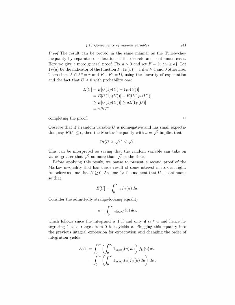
4.15 Convergence of random variables 241

Proof The result can be proved in the same manner as the Tchebychev

inequality by separate consideration of the discrete and continuous cases.

Here we give a more general proof. Fix a > 0 and set F = u : u ≥ a. Let

1F (u) be the indicator of the function F , 1F (u) = 1 if u ≥ a and 0 otherwise.

Then since F ∩ F c = ∅ and F ∪ F c = Ω, using the linearity of expectation

and the fact that U ≥ 0 with probability one:

E[U ] = E[U(1F (U) + 1F c(U))]

= E[U(1F (U))] + E[U(1F c(U))]

≥ E[U(1F (U))] ≥ aE[1F (U)]

= aP (F ).

completing the proof. 2

Observe that if a random variable U is nonnegative and has small expecta-

tion, say E[U ] ≤ ǫ, then the Markov inequality with a =√

ǫ implies that

Pr(U ≥ √ǫ ) ≤ √

ǫ.

This can be interpreted as saying that the random variable can take on

values greater that√

ǫ no more than√

ǫ of the time.

Before applying this result, we pause to present a second proof of the

Markov inequality that has a side result of some interest in its own right.

As before assume that U ≥ 0. Assume for the moment that U is continuous

so that

E[U ] =

∫ ∞

0ufU (u) du.

Consider the admittedly strange-looking equality

u =

∫ ∞

01[α,∞)(u) dα,

which follows since the integrand is 1 if and only if α ≤ u and hence in-

tegrating 1 as α ranges from 0 to u yields u. Plugging this equality into

the previous integral expression for expectation and changing the order of

integration yields

E[U ] =

∫ ∞

0

(∫ ∞

01[α,∞)(u) dα

)fU(u) du

=

∫ ∞

0

(∫ ∞

01[α,∞)(u)fU (u) du

)dα,

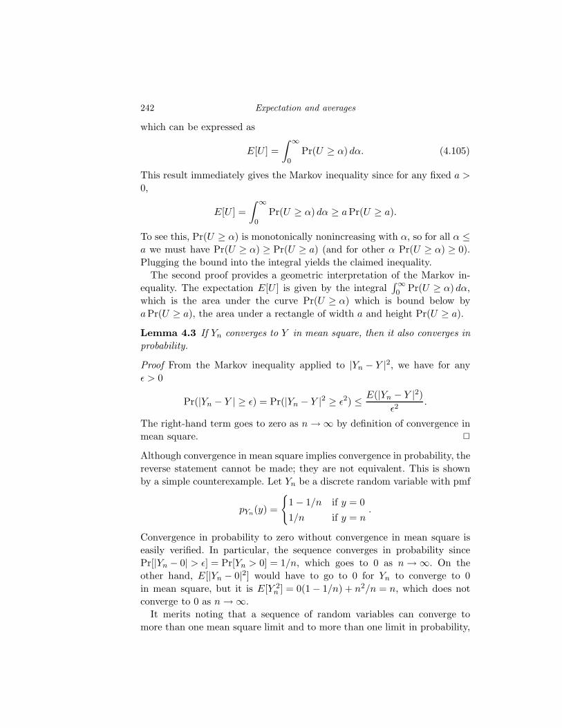
242 Expectation and averages

which can be expressed as

E[U ] =

∫ ∞

0Pr(U ≥ α) dα. (4.105)

This result immediately gives the Markov inequality since for any fixed a >

0,

E[U ] =

∫ ∞

0Pr(U ≥ α) dα ≥ aPr(U ≥ a).

To see this, Pr(U ≥ α) is monotonically nonincreasing with α, so for all α ≤a we must have Pr(U ≥ α) ≥ Pr(U ≥ a) (and for other α Pr(U ≥ α) ≥ 0).

Plugging the bound into the integral yields the claimed inequality.

The second proof provides a geometric interpretation of the Markov in-

equality. The expectation E[U ] is given by the integral∫∞0 Pr(U ≥ α) dα,

which is the area under the curve Pr(U ≥ α) which is bound below by

aPr(U ≥ a), the area under a rectangle of width a and height Pr(U ≥ a).

Lemma 4.3 If Yn converges to Y in mean square, then it also converges in

probability.

Proof From the Markov inequality applied to |Yn − Y |2, we have for any

ǫ > 0

Pr(|Yn − Y | ≥ ǫ) = Pr(|Yn − Y |2 ≥ ǫ2) ≤ E(|Yn − Y |2)ǫ2

.

The right-hand term goes to zero as n → ∞ by definition of convergence in

mean square. 2

Although convergence in mean square implies convergence in probability, the

reverse statement cannot be made; they are not equivalent. This is shown

by a simple counterexample. Let Yn be a discrete random variable with pmf

pYn(y) =

1 − 1/n if y = 0

1/n if y = n.

Convergence in probability to zero without convergence in mean square is

easily verified. In particular, the sequence converges in probability since

Pr[|Yn − 0| > ǫ] = Pr[Yn > 0] = 1/n, which goes to 0 as n → ∞. On the

other hand, E[|Yn − 0|2] would have to go to 0 for Yn to converge to 0

in mean square, but it is E[Y 2n ] = 0(1 − 1/n) + n2/n = n, which does not

converge to 0 as n → ∞.

It merits noting that a sequence of random variables can converge to

more than one mean square limit and to more than one limit in probability,

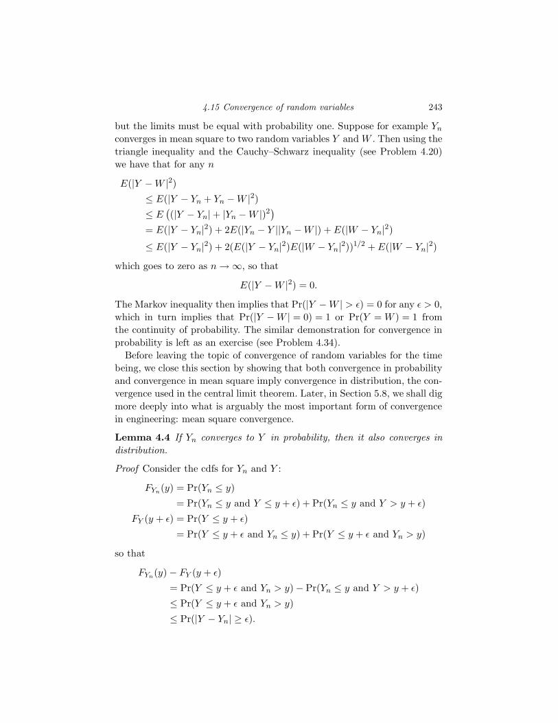
4.15 Convergence of random variables 243

but the limits must be equal with probability one. Suppose for example Yn

converges in mean square to two random variables Y and W . Then using the

triangle inequality and the Cauchy–Schwarz inequality (see Problem 4.20)

we have that for any n

E(|Y − W |2)≤ E(|Y − Yn + Yn − W |2)≤ E

((|Y − Yn| + |Yn − W |)2

)

= E(|Y − Yn|2) + 2E(|Yn − Y ||Yn − W |) + E(|W − Yn|2)≤ E(|Y − Yn|2) + 2(E(|Y − Yn|2)E(|W − Yn|2))1/2 + E(|W − Yn|2)

which goes to zero as n → ∞, so that

E(|Y − W |2) = 0.

The Markov inequality then implies that Pr(|Y − W | > ǫ) = 0 for any ǫ > 0,

which in turn implies that Pr(|Y − W | = 0) = 1 or Pr(Y = W ) = 1 from

the continuity of probability. The similar demonstration for convergence in

probability is left as an exercise (see Problem 4.34).

Before leaving the topic of convergence of random variables for the time

being, we close this section by showing that both convergence in probability

and convergence in mean square imply convergence in distribution, the con-

vergence used in the central limit theorem. Later, in Section 5.8, we shall dig

more deeply into what is arguably the most important form of convergence

in engineering: mean square convergence.

Lemma 4.4 If Yn converges to Y in probability, then it also converges in

distribution.

Proof Consider the cdfs for Yn and Y :

FYn(y) = Pr(Yn ≤ y)

= Pr(Yn ≤ y and Y ≤ y + ǫ) + Pr(Yn ≤ y and Y > y + ǫ)

FY (y + ǫ) = Pr(Y ≤ y + ǫ)

= Pr(Y ≤ y + ǫ and Yn ≤ y) + Pr(Y ≤ y + ǫ and Yn > y)

so that

FYn(y) − FY (y + ǫ)

= Pr(Y ≤ y + ǫ and Yn > y) − Pr(Yn ≤ y and Y > y + ǫ)

≤ Pr(Y ≤ y + ǫ and Yn > y)

≤ Pr(|Y − Yn| ≥ ǫ).

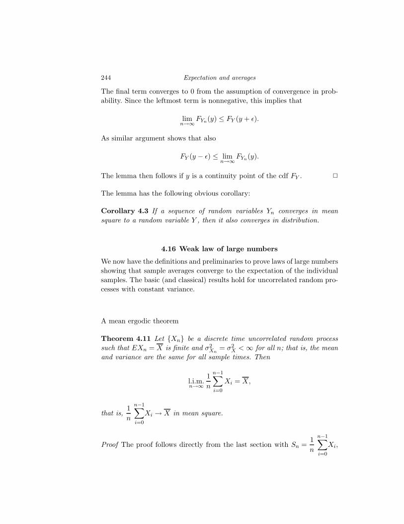
244 Expectation and averages

The final term converges to 0 from the assumption of convergence in prob-

ability. Since the leftmost term is nonnegative, this implies that

limn→∞

FYn(y) ≤ FY (y + ǫ).

As similar argument shows that also

FY (y − ǫ) ≤ limn→∞

FYn(y).

The lemma then follows if y is a continuity point of the cdf FY . 2

The lemma has the following obvious corollary:

Corollary 4.3 If a sequence of random variables Yn converges in mean

square to a random variable Y , then it also converges in distribution.

4.16 Weak law of large numbers

We now have the definitions and preliminaries to prove laws of large numbers

showing that sample averages converge to the expectation of the individual

samples. The basic (and classical) results hold for uncorrelated random pro-

cesses with constant variance.

A mean ergodic theorem

Theorem 4.11 Let Xn be a discrete time uncorrelated random process

such that EXn = X is finite and σ2Xn

= σ2X < ∞ for all n; that is, the mean

and variance are the same for all sample times. Then

l.i.m.n→∞

1

n

n−1∑

i=0

Xi = X,

that is,1

n

n−1∑

i=0

Xi → X in mean square.

Proof The proof follows directly from the last section with Sn =1

n

n−1∑

i=0

Xi,

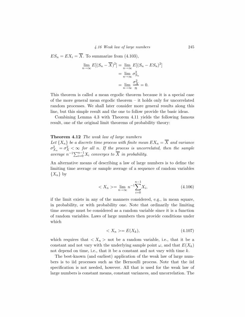
4.16 Weak law of large numbers 245

ESn = EXi = X. To summarize from (4.103),

limn→∞

E[(Sn − X)2] = limn→∞

E[(Sn − ESn)2]

= limn→∞

σ2Sn

= limn→∞

σ2X

n= 0.

This theorem is called a mean ergodic theorem because it is a special case

of the more general mean ergodic theorem – it holds only for uncorrelated

random processes. We shall later consider more general results along this

line, but this simple result and the one to follow provide the basic ideas.

Combining Lemma 4.3 with Theorem 4.11 yields the following famous

result, one of the original limit theorems of probability theory:

Theorem 4.12 The weak law of large numbers

Let Xn be a discrete time process with finite mean EXn = X and variance

σ2Xn

= σ2X < ∞ for all n. If the process is uncorrelated, then the sample

average n−1∑n−1

i=0 Xi converges to X in probability.

An alternative means of describing a law of large numbers is to define the

limiting time average or sample average of a sequence of random variables

Xn by

< Xn >= limn→∞

n−1n−1∑

i=0

Xi, (4.106)

if the limit exists in any of the manners considered, e.g., in mean square,

in probability, or with probability one. Note that ordinarily the limiting

time average must be considered as a random variable since it is a function

of random variables. Laws of large numbers then provide conditions under

which

< Xn >= E(Xk), (4.107)

which requires that < Xn > not be a random variable, i.e., that it be a

constant and not vary with the underlying sample point ω, and that E(Xk)

not depend on time, i.e., that it be a constant and not vary with time k.

The best-known (and earliest) application of the weak law of large num-

bers is to iid processes such as the Bernoulli process. Note that the iid

specification is not needed, however. All that is used for the weak law of

large numbers is constant means, constant variances, and uncorrelation. The

246 Expectation and averages

actual distributions could be time-varying and dependent within these con-

straints. The weak law is called weak because convergence in probability is

one of the weaker forms of convergence. Convergence of individual realiza-

tions of the random process is not assured. This could be very annoying

because in many practical engineering applications, we have only one real-

ization to work with (i.e., only one ω), and we need to calculate averages

that converge as determined by actual calculations, e.g., with a computer.

The strong law of large numbers considers convergence with probability

one. Such strong theorems are much harder to prove, but fortunately are

satisfied in most engineering situations.

The astute reader may have noticed the remarkable difference in behavior

caused by the apparently slight change of division by√

n instead of n when

normalizing sums of iid random variables. In particular, if Xn is a zero-

mean process with unit variance, then the weighted sum n−(1/2)∑n−1

k=0 Xk

converges to a Gaussian random variable in some sense because of the cen-

tral limit theorem, whereas the weighted sum n−1∑n−1

k=0 Xk converges to a

constant, the mean of the individual random variables!

4.17 ⋆Strong law of large numbers

The strong law of large numbers replaces the convergence in probability

of the weak law with convergence with probability one. It will shortly be

shown that convergence with probability one implies convergence in proba-

bility, so the “strong” law is indeed stronger than the “weak” law. Although

the two terms sound the same, they are really quite different. Convergence

with probability one applies to individual realizations of the random process,

whereas convergence in probability does not. Convergence with probability

one is closer to the usual definition of convergence of a sequence of num-

bers since it says that for each sample point ω, the limiting sample average

limn→∞ n−1∑∞

n=1 Xn exists in the usual sense for all ω in a set of proba-

bility one. Although convergence with probability one is a more satisfying

notion of convergence, it is notably harder to prove than the weaker result.

Hence we consider only the special case of iid sequences, where the added

difficulty is moderate. In this section convergence with probability one is

considered and a strong law of large numbers is proved. The key new tools

are the Borel–Cantelli lemma, which provides a condition ensuring conver-

gence with probability one, and the Chernoff inequality, an improvement on

the Tchebychev inequality.

4.17 ⋆Strong law of large numbers 247

Lemma 4.5 If Yn converges to Y with probability one, then it also converges

in probability.

Proof Given an ǫ > 0, define the sequence of sets

Gn(ǫ) = ω : |Yn(ω) − Y (ω)| ≥ ǫFn(ǫ) = ω : |Ym(ω) − Y (ω)| ≥ ǫ for some m ≥ n

=⋃

m≥n

Gm(ǫ).

Thus Gn(ǫ) ⊂ Fn(ǫ) and the Fn(ǫ) form a decreasing sequence of sets as n

grows, that is, Fn ⊂ Fn−1 for all n. Thus from the continuity of probability,

limn→∞

Pr(Fn(ǫ)) = Pr(

limn→∞

Fn(ǫ))

= Pr

( ∞⋂

n=1

Fn(ǫ)

)

= Pr

∞⋂

n=1

⋃

m≥n

Gm(ǫ)

.

If ω ∈ B =⋂∞

n=1

⋃m≥n Gm(ǫ), then for every value of n there must exist

an m ≥ n for which |Ym(ω) − Y (ω)| ≥ ǫ, which means that Ym(ω) does not

converge to Y (ω). Since Yn is assumed to converge to Y with probability

one, Pr(B) = 0 and hence

limn→∞

Pr(Gn(ǫ)) ≤ limn→∞

Pr(Fn(ǫ)) = Pr(B) = 0.

Convergence in probability does not imply convergence with probability

one; i.e., they are not equivalent. This can be shown by counterexample

(Problem 4.36). There is, however, a test that can be applied to determine

convergence with probability one. The result is one form of a result known

as the first Borel–Cantelli lemma.

Lemma 4.6 Yn converges to Y with probability one if for any ǫ > 0

∞∑

n=1

Pr(|Yn − Y | > ǫ) < ∞. (4.108)

Proof Consider two collections of bad sequences. Let F (ǫ) be the set of all ω

such that the corresponding sequence Yn(ω) does not satisfy the convergence

criterion, i.e.,

F (ǫ) = ω : |Yn − Y | > ǫ, for some n ≥ N, for any N < ∞.

F (ǫ) is the set of points for which the sequence does not converge. Consider

248 Expectation and averages

also the simpler sets where things look bad at a particular time:

Fn(ǫ) = ω : |Yn − Y | > ǫ.

The complicated collection of points with nonconvergent sequences can be

written as a subset of the union of all of the simpler sets:

F (ǫ) ⊂∞⋃

n≥N

Fn(ǫ)∆= GN (ǫ))

for any finite N . This in turn implies that

Pr(F (ǫ)) ≤ Pr(

∞⋃

n≥N

Fn(ǫ)).

From the union bound this implies that

Pr(F (ǫ)) ≤∞∑

n=N

Pr(Fn(ǫ)).

By assumption

∞∑

n=0

Pr(Fn(ǫ)) < ∞,

which implies that

limN→∞

∞∑

n=N

Pr(Fn(ǫ)) = 0

and hence Pr(F (ǫ)) = 0, proving the result. 2

Convergence with probability one does not imply – nor is it implied by –

convergence in mean square. This can be shown by counterexamples (Prob-

lem 4.36).

We now apply this result to sample averages to obtain a strong law of

large numbers for an iid random process Xn. For simplicity we focus on

a zero-mean Gaussian iid process and prove that with probability one

limn→∞

Sn = 0

where

Sn =1

n

n−1∑

k=0

Xk.

4.17 ⋆Strong law of large numbers 249

Assuming zero-mean does not lose any generality since if this result is true,

the result for nonzero-mean m follows immediately by applying the zero-

mean result to the zero-mean process Xn − m.The approach is to use the Borel–Cantelli lemma with Yn = Sn and Y =

0 = E[Xn] and hence the immediate problem is to bound Pr(|Sn| > ǫ) in

such a way that the sum over n will be finite. The Tchebychev inequality

does not work here as it would yield a sum

σ2X

∞∑

n=1

1

n,

which is not finite. A better upper bound than Tchebychev is needed. This is

provided by a different application of the Markov inequality. Given a random

variable Y , fix a λ > 0 and observe that Y > y if and only if eλY > eλy.

Application of the Markov inequality then yields

Pr(Y > y) = Pr(eλY > eλy) = Pr(eλ(Y −y) > 1)

≤ E[eλ(Y −y)]. (4.109)

This inequality is called the Chernoff inequality and it provides the needed

bound.

Applying the Chernoff inequality yields for any λ > 0

Pr(|Sn| > ǫ) = Pr(Sn > ǫ) + Pr(Sn < −ǫ)

= Pr(Sn > ǫ) + Pr(−Sn > ǫ)

≤ E[eλ(Sn−ǫ)] + E[eλ(−Sn−ǫ)]

= e−λǫ(E[eλSn ] + E[e−λSn ]

)

= e−λǫ (MSn(λ) + MSn(−λ)) .

These moment-generating functions are easily found from Lemma 4.1 to be

E[eγSn ] = MnX

(γ

n

), (4.110)

where MX(ju) = E[ejuX ] is the common characteristic function of the iid Xi

and MX(w) is the corresponding moment-generating function. Combining

these steps yields the bound

Pr(|Sn| > ǫ) ≤ e−λǫ

(Mn

X

(λ

n

)+ Mn

X

(−λ

n

)). (4.111)

250 Expectation and averages

So far λ > 0 is completely arbitrary. We can choose a different λ for each

n. Choosing λ = nǫ/σ2X yields

Pr(|Sn| > ǫ) ≤ e−n ǫ2

σ2X

(Mn

X

(ǫ

σ2X

)+ Mn

X

(− ǫ

σ2X

)). (4.112)

Plugging in the form for the Gaussian moment-generating function

MX(w) = ew2σ2X/2 yields

Pr(|Sn| > ǫ) ≤ 2e−nǫ2/σ2X

(e(ǫ/σ2

X )2σ2X/2)n

= 2(e−ǫ2/2σ2

X

)n(4.113)

which has the form Pr(|Sn| > ǫ) ≤ 2βn for β < 1. Hence summing a geomet-

ric progression yields

∞∑

n=1

Pr(|Sn| > ǫ) ≤ 2∞∑

n=1

βn = 2β

1 − β< ∞, (4.114)

which completes the proof for the iid Gaussian case.

The non-Gaussian case can be handled by combining the above approach

with the approximation of (4.15). The bound for the Borel–Cantelli limit

need only be demonstrated for small ǫ since if it is true for small ǫ it must

also be true for large ǫ. For small ǫ, however, (4.15) implies that MX(±ǫ/σ2X)

in (4.112) can be written as 1 + ǫ2/2σ2X + o(ǫ2/2σ2

X) which is arbitrarily

close to eǫ2/2σ2X for sufficiently small ǫ, and the proof is completed as above.

The following theorem summarizes the results of this section.

Theorem 4.13 Strong law of large numbers

Given an iid process Xn with finite mean E[X] and variance, then

limn→∞

1

n

n−1∑

k=0

Xk = E[X] with probability one. (4.115)

4.18 Stationarity

Stationarity properties

In the development of the weak law of large numbers we made two as-

sumptions on a random process Xt; t ∈ Z: that the mean EXt of the

process did not depend on time and that the covariance function had the

form KX(t, s) = σ2Xδt−s.

The assumption of a constant mean, independent of time, is an example

4.18 Stationarity 251

of a stationarity property in the sense that it assumes that some property

describing a random process does not vary with time (or is time-invariant).

The process itself is not usually “stationary” in the usual literal sense of

remaining still, but attributes of the process, such as the first moment in

this case, can remain still in the sense of not changing with time. In the

mean example we can also express this as

EXt = EXt+τ ; all t, τ, (4.116)

which can be interpreted as saying that the mean of a random variable

at time t is not affected by a shift of any amount of time τ . Conditions

on moments can be thought of as weak stationarity properties since they

constrain only an expectation and not the distribution itself. Instead of

simply constraining a moment, we could make the stronger assumption of

constraining the marginal distribution. The assumption of a constant mean

would follow, for example, if the marginal distribution of the process, the

distribution of a single random variable Xt, did not depend on the sample

time t. Thus a sufficient (but not necessary) condition for ensuring that a

random process has a constant mean is that its marginal distribution PXt

satisfies the condition

PXt = PXt+τ ; all t, τ. (4.117)

This will be true, for example, if the same relation holds with the distribution

replaced by cdf’s, pdf’s, or pmf’s. If a process meets this condition, it is

said to be first-order stationary. For example, an iid process is clearly first-

order stationary. The word stationary refers to the fact that the first-order

distribution (in this case) does not change with time, i.e., it is not affected

by shifting the sample time by an amount τ .

Next consider the covariance used to prove the weak law of large numbers.

It has a very special form in that it is the variance if the two sample times

are the same, and zero otherwise. This class of constant mean, constant

variance, and uncorrelated processes is admittedly an unusual case. A more

general class of processes which will share many important properties with

this very special case is formed by requiring a mean and variance that do

not change with time, but easing the restriction on the covariance. We say

that a random process is weakly stationary or stationary in the weak sense

if EXt does not depend on t, σ2Xt

does not depend on t, and the covariance

KX(t, s) depends on t and s only through the difference t − s, that is, if

KX(t, s) = KX(t + τ, s + τ) (4.118)

252 Expectation and averages

for all t, s, τ for which s, s + τ, t, t + τ ∈ T . When this is true, it is often

expressed by writing

KX(t, t + τ) = KX(τ). (4.119)

for all t, τ such that t, t + τ ∈ T . A function of two variables of this type is

said to be Toeplitz [36, 31]. Much of the theory of weakly stationary processes

follows from the theory of Toeplitz forms.

If we form a covariance matrix by sampling such a covariance function,

then the matrix (called a Toeplitz matrix) will have the property that all

elements on any fixed diagonal of the matrix will be equal. For example,

the (3,5) element will be the same as the (7,9) element since 5 − 3 = 9 − 7.

Thus, for example, if the sample times are 0, 1, . . . , n − 1, then the covariance

matrix is KX(k, j) = KX(j − k); k = 0, 1, . . . , n − 1, j = 0, 1, . . . , n − 1 or

KX(0) KX(1) KX(2) . . . KX(n − 1)

KX(−1) KX(0) KX(1)

KX(−2) KX(−1) KX(0)...

.... . .

KX(−(n − 1)) . . . KX(0)

As in the case of constant mean, the adjective weakly refers to the fact

that the constraint is placed on the moments and not on the distributions.

Mimicking the earlier discussion, we could make a stronger assumption that

is sufficient to ensure weak stationarity. A process is said to be second-order

stationary if the pairwise distributions are not affected by shifting; that is, if

analogous to the moment condition (4.118) we make the stronger assumption

that

PXt,Xs = PXt+τ ,Xs+τ ; all t, s, τ. (4.120)

Observe that second-order stationarity implies first-order since the marginals

can be computed from the joints. The class of iid processes is second-order

stationary since the joint probabilities are products of the marginals, which

do not depend on time.

There are a variety of such stationarity properties that can be defined,

but weakly stationary is one of the two most important for two reasons.

The first reason will be seen shortly – combining weak stationarity with an

asymptotic version of uncorrelated gives a more general law of large num-

bers than the ones derived previously. The second reason will be seen in the

next chapter: if a covariance depends only on a single argument (the differ-

ence of the sample times), then it will have an ordinary Fourier transform.

4.18 Stationarity 253

Transforms of correlation and covariance functions provide useful analysis

tools for stochastic systems.

Before proceeding it is useful to consider the other most important sta-

tionarity property: strict stationarity (sometimes the adjective “strict” is

omitted). As the notion of weak stationary can be considered as a gener-

alization of uncorrelated, the notion of strict stationary can be considered

as a generalization of iid: if a process is iid, the probability distribution of

a k-dimensional random vector Xn,Xn+1, . . . ,Xn+k−1 does not depend on

the starting time of the collection of samples, i.e., for an iid process we have

that

PXn,Xn+1,...,Xn+k−1= PXn+m,Xn+m+1,...,Xn+m+k−1

(x), all n, k,m. (4.121)

This property can be interpreted as saying that the probability of any event

involving a finite collection of samples of the random process does not depend

on the starting time n of the samples and hence on the definition of time

0. Alternatively, these joint distributions are not affected by shifting the

samples by a common amount m. In the simple Bernoulli process case this

means things like

pXn(0) = pX0(0) = 1 − p, all n

pXn,Xk(0, 1) = pX0,Xk−n

(0, 1) = p(1 − p), all n, k

pXn,Xk,Xl(0, 1, 0) = pX0,Xk−n,Xl−n

(0, 1, 0) = (1 − p)2p, all n, k,m,

and so on. Note that the relative sample times stay the same, that is, the

differences between the sample times are preserved, but all of the samples

together are shifted without changing the probabilities. A process need not

be iid to possess the property of joint probabilities being unaffected by shifts,

so we formalize this idea with a definition.

A discrete time random process Xn is said to be stationary or strictly

stationary or stationary in the strict sense if (4.121) holds. We have argued

that a discrete alphabet iid process is an example of a stationary random

process. This definition extends immediately to continuous alphabet discrete

time processes by replacing the pmf’s by pdf’s. Both cases can be combined

by using cdf’s or the distributions. Hence we can make a more general def-

inition for discrete time processes: a discrete time random process Xn is

said to be stationary if

PXn,Xn+1,...,Xn+k−1= PXn+m,Xn+m+1,...,Xn+m+k−1

, all k, n,m. (4.122)

This will hold if the corresponding formula holds for pmf’s, pdf’s, or cdf’s.

For example, any iid random process is stationary.

254 Expectation and averages

Generalizing the definition to include continuous time random processes

requires only a little more work, much like that used to describe the Kol-

mogorov extension theorem. We would like all joint distributions involving a

finite collection of samples to be independent of the starting time or, equiva-

lently, to be unaffected by shifts. The following general definition does this.

It reduces to the previous definition when the process is a discrete time

process.

A random process Xt; t ∈ T is stationary if

PXt0 ,Xt1 ,...,Xtk−1= PXt0−τ ,Xt1−τ ,...,Xtk−1−τ , all k, t0, t1, . . . , tk−1, τ. (4.123)

The word “all” above must be interpreted with care; it means all choices of

dimension k, sample times t0, . . . , tk−1, and shift τ for which the equation

makes sense, e.g., k must be a positive integer and ti ∈ T and ti − τ ∈ T for

i = 0, . . . , k − 1.

It should be obvious that strict stationarity implies weak stationarity

since it implies that PXt does not depend on t, and hence the mean com-

puted from this distribution does not depend on t, and it implies that

PXt,Xs = PXt−s,X0 and hence KX(t, s) = KX(t − s, 0). The converse is gen-

erally not true – knowing that two moments are unaffected by shifts does not

in general imply that all finite-dimensional distributions will be unaffected

by shifts. This is why weak stationarity is indeed a “weaker” definition of

stationarity. There is, however, one extremely important case where weak

stationarity is sufficient to ensure strict stationarity – the case of Gaus-

sian random processes. We shall not construct a careful proof of this fact

because it is a notational mess that obscures the basic idea, which is actu-

ally rather easy to describe. A Gaussian process Xt; t ∈ T is completely

characterized by knowledge of its mean function mt; t ∈ T and its co-

variance function KX(t, s); t, s ∈ T . All joint pdf’s for all possible finite

collections of sample times are expressed in terms of these two functions.

If the process is known to be weakly stationary, then mt = m for all t, and

KX(t, s) = KX(t − s, 0) for all t, s. This implies that all of the joint pdf’s

will be unaffected by a time shift, since the mean vector stays the same and

the covariance matrix depends only on the relative differences of the sample

times, not on where they begin. Thus in this special case, knowing a process

is weakly stationary is sufficient to conclude it is stationary. However, in

general, stationarity can be difficult to prove, even for simple processes.

⋆Strict stationarity In fact the above is not the definition of stationarity

used in the mathematical and statistical literature, but it is equivalent to

4.18 Stationarity 255

it. We pause for a moment to describe the more fundamental (but abstract)

definition and its relation to the above definition. The reader should keep

in mind that it is the above definition that is the important one in practice:

it is the definition that is almost always used to verify that a process is

stationary or not.

To state the alternative definition, recall that a random process Xt; t ∈T can be considered to be a mapping from a probability space (Ω,F , P ) into

a space of sequences or waveforms xt; t ∈ T and that the inverse image

formula implies a probability measure called a process distribution, say PX ,

on this complicated space, i.e., PX(F ) = PX(xt; t ∈ T : xt; t ∈ T ∈F) = P (ω : Xt(ω); t ∈ T ∈ F). The abstract definition of stationarity

places a condition on the process distribution: a random process Xt; t ∈ T is stationary if the process distribution PX is unchanged by shifting, that is,

if

PX(xt; t ∈ T : xt; t ∈ T ∈ F)= PX(xt; t ∈ T : xt+τ ; t ∈ T ∈ F); all F, τ. (4.124)

The only difference between the left- and right-hand side is that the right-

hand side takes every sample waveform and shifts it by a common amount

τ . If the abstract definition is applied to finite-dimensional events, that is,

events which actually depend only on a finite number of sample times, then

this definition reduces to that of (4.123). Conversely, it turns out that having

this property hold on all finite-dimensional events is enough to imply that

the property holds for all possible events, even those depending on an infinite

number of samples (such as the event one gets an infinite binary sequence

with exactly p limiting relative frequency of heads). Thus the two definitions

of strict stationarity are equivalent. The proof of this equivalence is one of the

classic results of the theory of random processes and requires tools beyond

those assumed for this book. The interested reader can find a thorough

development in [32]. The underlying idea is that the collection of all finite-

dimensional events generates the entire event space of the sample space

of all waveforms or sequences. Given a consistent set of probabilities on a

generating collection of events, it can be shown there must exist a probability

measure on the full event space that agrees with the given probabilities.

Why is stationarity important? Are processes that are not stationary in-

teresting? The answer to the first question is that this property leads to

the most famous of the law of large numbers, which will be quoted without

proof later. The answer to the second question is yes, nonstationary processes

play an important role in theory and practice, as will be seen by example.

256 Expectation and averages

In particular, some nonstationary processes will have a form of a law of

large numbers, and others will have no such property, yet be quite useful in

modeling real phenomena. Keep in mind that strict stationarity is stronger

than weak stationarity. Thus if a process is not even weakly stationary then

the process is also not strictly stationary. Two examples of nonstationary

processes already encountered are the binomial counting process and the

discrete time Wiener process. These processes have marginal distributions

which change with time and hence the processes cannot be stationary. We

shall see in Chapter 5 that these processes are also not weakly stationary.

4.19 Asymptotically uncorrelated processes

We close this chapter with a generalization of the mean ergodic theorem

and the weak law of large numbers that demonstrates that weak stationarity

plus an asymptotic form of uncorrelation is sufficient to yield a weak law of

large numbers by a fairly modest variation of the earlier proof. The class of

asymptotically uncorrelated processes is often encountered in practice. Only

the result itself is important; the proof is a straightforward but tedious

extension of the proof for the uncorrelated case.

An advantage of the more general result over the result for uncorrelated

discrete time random processes is that it extends in a sensible way to con-

tinuous time processes.

A discrete time weakly stationary process Xn; n ∈ Z is said to be

asymptotically uncorrelated if its covariance function is absolutely summable,

that is, if

∞∑

k=−∞|KX(k)| < ∞. (4.125)

This condition implies that also

limk→∞

KX(k) = 0, (4.126)

and hence the property (4.125) can be considered as a weak form of un-

correlation, a generalization of the fact that a weakly stationary process is

uncorrelated if KX(k) = 0 when k 6= 0. If a process is uncorrelated, then

Xn and Xn+k are uncorrelated random variables for all nonzero k; if it is

asymptotically uncorrelated, the correlation between the two random vari-

ables decreases to zero as k grows. We use (4.125) rather than the weaker

(4.126) as the definition as it also ensures the existence of a Fourier trans-

4.19 Asymptotically uncorrelated processes 257

form of KX , which will be useful later. It also simplifies the proof of the

resulting law of large numbers.

Theorem 4.14 A mean ergodic theorem

Let Xn be a weakly stationary asymptotically uncorrelated discrete time

random process such that EXn = X is finite and σ2Xn

= σ2X < ∞ for all n.

Then .

l.i.m.n→∞

1

n

n−1∑

i=0

Xi = X,

that is,1

n

n−1∑

i=0

Xi → X in mean square.

Note that the theorem is indeed a generalization of the previous mean er-

godic theorem since a weakly stationary uncorrelated process is trivially an

asymptotically uncorrelated process. Note also that the Tchebychev inequal-

ity and this theorem immediately imply convergence in probability and hence

establish a weak law of large numbers for weakly stationary asymptotically

uncorrelated processes. Common examples of asymptotically uncorrelated

processes are processes with exponentially decreasing covariance, i.e., of the

form KX(k) = σ2Xρ|k| for ρ < 1.

⋆Proof for the asymptotically uncorrelated case

Proof Exactly as in the proof of Theorem 4.11 we have with Sn =

n−1∑n−1

i=0 Xi that

E[(Sn − X)2] = E[(Sn − ESn)2] = σ2Sn

.

From (4.101) we have that

σ2Sn

= n−2n−1∑

i=0

n−1∑

j=0

KX(i − j). (4.127)

This sum can be rearranged as in Lemma B.1 of Appendix B as

σ2Sn

=1

n

n−1∑

k=−n+1

(1 − |k|

n

)KX(k). (4.128)

258 Expectation and averages

From Lemma B.2

limn→∞

n−1∑

k=−n+1

(1 − |k|

n

)KX(k) =

∞∑

k=−∞KX(k),

which is finite by assumption, hence dividing by n yields

limn→∞

1

n

n−1∑

k=−n+1

(1 − |k|

n

)KX(k) = 0

which completes the proof. 2

A similar definition applies to continuous time processes. We say that

X(t); t ∈ ℜ is asymptotically uncorrelated if its covariance function is ab-

solutely integrable,∫ ∞

−∞|KX(τ)| < ∞, (4.129)

which implies that

limτ→∞

KX(τ) = 0. (4.130)

No sensible continuous time random process can be uncorrelated (why not?),

but many are asymptotically uncorrelated. A sample or time average can be

defined for a continuous time process by replacing the sum operation by an

integral, that is, by

ST =1

T

∫ T

0X(t) dt. (4.131)

For the moment we ignore the technical difficulties that must be considered

to assure that the integral exists in a suitable fashion. Suffice it to say that

an integral can be considered as a limit of sums, and we have seen ways to

make such limits of random variables precise. We will return to this issue

with more care in Section 5.8. The definition of weakly stationary extends

immediately to continuous time processes. The following result can be proved

by extending the discrete time result to continuous time and integrals.

Theorem 4.15 A mean ergodic theorem

Let X(t) be a weakly stationary asymptotically uncorrelated continuous

time random process such that EX(t) = X is finite and σ2X(t) = σ2

X < ∞for all t. Then .

l.i.m.T→∞

1

T

∫ T

0X(t) dt = X,

4.20 Problems 259

that is,1

T

∫ T

0X(t) dt → X in mean square.

As in the discrete time case, convergence in mean square immediately im-

plies converges in probability, but much additional work is required to prove

convergence with probability one (when such convergence indeed holds).

Also as in the discrete case, we can define a limiting time average

< X(t) >= limT→∞

1

T

∫ T

0X(t) dt (4.132)

and interpret the law of large numbers as stating that the time average

< X(t) > exists in some sense and equals the expectation.

4.20 Problems

1. Wanda is going shopping for mystery books to take on a trip. She will spend

X hours in the bookstore, where X is a discrete random variable equally likely

to take on values of 1, 2, 3, or 4. She will buy N books, where N is a discrete

random variable which depends on the amount of time she shops as described

by a conditional probability mass function

pN |X(n|k) =1

k; n = 1, 2, . . . , k.

(a) Find the joint pmf of X and N .

(b) Find the marginal pmf for N .

(c) Find the conditional pmf of X given that N = 2.

(d) Suppose you know that Wanda bought at least two but not more than three

books. Find the conditional mean and variance of X given this information.

(e) The cost of each book is a random variable (independent of all the other

random variables in the problem) with mean 3. What is the expected value

of Wanda’s total expenditure?

2. The Cauchy pdf is defined by

fX(x) =1

π

1

1 + x2; x ∈ ℜ.

Find EX. Hint: this is a trick question. Check the definition of Riemann integra-

tion over (−∞,∞) before deciding on a final answer.

3. Suppose that Z is a discrete random variable with probability mass function

pZ(k) = Cak

(1 + a)k+1, k = 0, 1, . . .

(This is sometimes called “Pascal’s distribution.”) Find the constant C and the

mean, characteristic function, and variance of Z.

260 Expectation and averages

4. State and prove the fundamental theorem of expectation for the case where a dis-

crete random variable X is defined on a probability space where the probability

measure is described by a pdf f .

5. Given the setup of Problem 3.10:

(a) Find E(X) and E(XY ).

(b) Find the conditional expectation E(Y |X = x). For what value of x is this

maximized?

(c) Let A denote the event X2 ≥ Y . Find P (A) and E(XY |A ).

6. Suppose that X is a random variable with pdf fX(α) and characteristic function

MX(ju) = E[ejuX ]. Define the new random variable Y = aX + b, where both a

and b are positive constants. Find the pdf fY and characteristic function MY (ju)

in terms of fX and MX , respectively.

7. X , Y and Z are iid Gaussian random variables with N (1, 1) distributions.

Define the random variables:

V = 2X + Y

W = 3X − 2Z + 5.

(a) Find E[V W ].

(b) Find the two parameters that completely specify the random variable V + W.

(c) Find the characteristic function of the random vector [V W ]t, where t denotes

“transpose.”

(d) Find the linear estimator V (W ) of V, given W .

(e) Find the optimal (smallest MSE) affine estimator V (W ) of V, given W . In

particular, find a and b such that V (W ) = aW + b yields the minimum

MSE = E[(V − V (W ))2]

(f) Is this an optimal estimator? Why?

(g) The zero-mean random variables X − X, Y − Y and Z − Z are the inputs

to a black box. There are two outputs, A and B. It is determined that the

covariance matrix of the vector of its outputs [A B]t should be

ΛAB =

[3 2

2 5

].

Find expressions for A and B in terms of the black box inputs so that this

is in fact the case (design the black box). Your answer does not necessarily

have to be unique.

(h) You are told that a different black box results in an output vector [C D]t

with the following covariance matrix:

ΛCD =

[2 0

0 7

].

How much information about output C does output D give you? Briefly but

fully justify your answer.

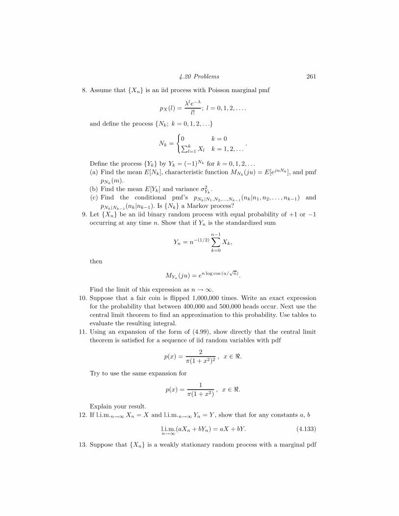
4.20 Problems 261

8. Assume that Xn is an iid process with Poisson marginal pmf

pX(l) =λle−λ

l!; l = 0, 1, 2, . . . .

and define the process Nk; k = 0, 1, 2, . . .

Nk =

0 k = 0∑k

l=1 Xl k = 1, 2, . . ..

Define the process Yk by Yk = (−1)Nk for k = 0, 1, 2, . . .

(a) Find the mean E[Nk], characteristic function MNk(ju) = E[ejuNk ], and pmf

pNk(m).

(b) Find the mean E[Yk] and variance σ2Yk

.

(c) Find the conditional pmf’s pNk|N1,N2,...,Nk−1(nk|n1, n2, . . . , nk−1) and

pNk|Nk−1(nk|nk−1). Is Nk a Markov process?

9. Let Xn be an iid binary random process with equal probability of +1 or −1

occurring at any time n. Show that if Yn is the standardized sum

Yn = n−(1/2)n−1∑

k=0

Xk,

then

MYn(ju) = en log cos (u/

√n).

Find the limit of this expression as n → ∞.

10. Suppose that a fair coin is flipped 1,000,000 times. Write an exact expression

for the probability that between 400,000 and 500,000 heads occur. Next use the

central limit theorem to find an approximation to this probability. Use tables to

evaluate the resulting integral.

11. Using an expansion of the form of (4.99), show directly that the central limit

theorem is satisfied for a sequence of iid random variables with pdf

p(x) =2

π(1 + x2)2, x ∈ ℜ.

Try to use the same expansion for

p(x) =1

π(1 + x2), x ∈ ℜ.

Explain your result.

12. If l.i.m.n→∞ Xn = X and l.i.m.n→∞ Yn = Y , show that for any constants a, b

l.i.m.n→∞

(aXn + bYn) = aX + bY. (4.133)

13. Suppose that Xn is a weakly stationary random process with a marginal pdf

262 Expectation and averages

fX(α) = 1 for 0 < α < 1 and a covariance function

KX(k) =1

12ρ|k|

for all integer k (ρ < 1). What is

l.i.m.n→∞

1

n

n∑

k=1

Xk ?

What is

l.i.m.n→∞

1

n2

n∑

k=1

Xk ?

14. If Xn is an uncorrelated process with constant first and second moments, does

it follow for an arbitrary function g that

l.i.m.n→∞

n−1n−1∑

i=0

g(Xi) = E[g(X)]?

(E[g(X)] denotes the unchanging value of E[g(Xn)].) Show that it does follow if

the process is iid.

15. Apply Problem 4.14 to indicator functions to prove that relative frequencies of

order n converge to pmf’s in mean square and in probability for iid random

processes. That is, if r(n)a is defined as in the chapter, then r

(n)a → pX(a) as

n → ∞ in both senses for any a in the range space of X .

16. Define the subsets of the real line

Fn =

r : |r| >

1

n

, n = 1, 2, . . .

and

F = 0.

Show that

F c =

∞⋃

n=1

Fn.

Use this fact, the Tchebychev inequality, and the continuity of probability to

show that if a random variable X has variance 0, then Pr(|X − EX | ≥ ǫ|) ≤ 0

independent of ∈ and hence Pr(X = EX) = 1.

17. True or false? Given a nonnegative random variable X , for any ǫ > 0 and a > 0:

Pr(X ≥ ǫ) ≤ E[eaX ]

eaǫ.

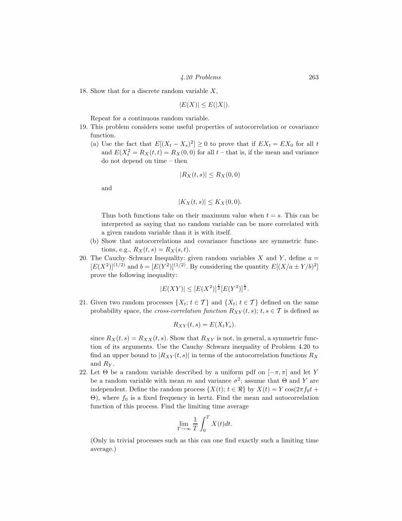
4.20 Problems 263

18. Show that for a discrete random variable X ,

|E(X)| ≤ E(|X |).

Repeat for a continuous random variable.

19. This problem considers some useful properties of autocorrelation or covariance

function.

(a) Use the fact that E[(Xt − Xs)2] ≥ 0 to prove that if EXt = EX0 for all t

and E(X2t = RX(t, t) = RX(0, 0) for all t – that is, if the mean and variance

do not depend on time – then

|RX(t, s)| ≤ RX(0, 0)

and

|KX(t, s)| ≤ KX(0, 0).

Thus both functions take on their maximum value when t = s. This can be

interpreted as saying that no random variable can be more correlated with

a given random variable than it is with itself.

(b) Show that autocorrelations and covariance functions are symmetric func-

tions, e.g., RX(t, s) = RX(s, t).

20. The Cauchy–Schwarz Inequality: given random variables X and Y , define a =

[E(X2)](1/2) and b = [E(Y 2)](1/2). By considering the quantity E[(X/a ± Y/b)2]

prove the following inequality:

|E(XY )| ≤ [E(X2)]12 [E(Y 2)]

12 .

21. Given two random processes Xt; t ∈ T and Xt; t ∈ T defined on the same

probability space, the cross-correlation function RXY (t, s); t, s ∈ T is defined as

RXY (t, s) = E(XtYs).

since RX(t, s) = RXX(t, s). Show that RXY is not, in general, a symmetric func-

tion of its arguments. Use the Cauchy–Schwarz inequality of Problem 4.20 to

find an upper bound to |RXY (t, s)| in terms of the autocorrelation functions RX

and RY .

22. Let Θ be a random variable described by a uniform pdf on [−π, π] and let Y

be a random variable with mean m and variance σ2; assume that Θ and Y are

independent. Define the random process X(t); t ∈ ℜ by X(t) = Y cos(2πf0t +

Θ), where f0 is a fixed frequency in hertz. Find the mean and autocorrelation

function of this process. Find the limiting time average

limT→∞

1

T

∫ T

0

X(t)dt.

(Only in trivial processes such as this can one find exactly such a limiting time

average.)

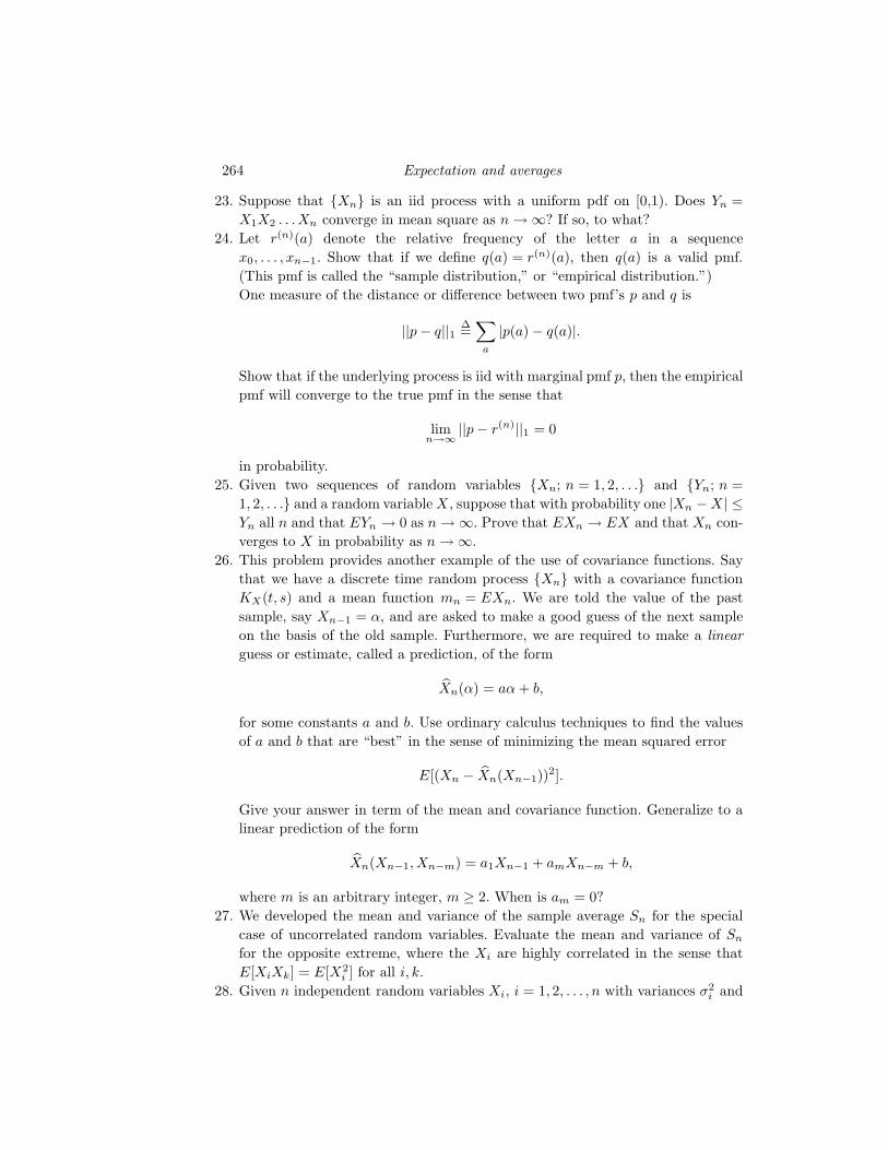
264 Expectation and averages

23. Suppose that Xn is an iid process with a uniform pdf on [0,1). Does Yn =

X1X2 . . .Xn converge in mean square as n → ∞? If so, to what?

24. Let r(n)(a) denote the relative frequency of the letter a in a sequence

x0, . . . , xn−1. Show that if we define q(a) = r(n)(a), then q(a) is a valid pmf.

(This pmf is called the “sample distribution,” or “empirical distribution.”)

One measure of the distance or difference between two pmf’s p and q is

||p − q||1 ∆=∑

a

|p(a) − q(a)|.

Show that if the underlying process is iid with marginal pmf p, then the empirical

pmf will converge to the true pmf in the sense that

limn→∞

||p − r(n)||1 = 0

in probability.

25. Given two sequences of random variables Xn; n = 1, 2, . . . and Yn; n =

1, 2, . . . and a random variable X , suppose that with probability one |Xn − X | ≤Yn all n and that EYn → 0 as n → ∞. Prove that EXn → EX and that Xn con-

verges to X in probability as n → ∞.

26. This problem provides another example of the use of covariance functions. Say

that we have a discrete time random process Xn with a covariance function

KX(t, s) and a mean function mn = EXn. We are told the value of the past

sample, say Xn−1 = α, and are asked to make a good guess of the next sample

on the basis of the old sample. Furthermore, we are required to make a linear

guess or estimate, called a prediction, of the form

Xn(α) = aα + b,

for some constants a and b. Use ordinary calculus techniques to find the values

of a and b that are “best” in the sense of minimizing the mean squared error

E[(Xn − Xn(Xn−1))2].

Give your answer in term of the mean and covariance function. Generalize to a

linear prediction of the form

Xn(Xn−1, Xn−m) = a1Xn−1 + amXn−m + b,

where m is an arbitrary integer, m ≥ 2. When is am = 0?

27. We developed the mean and variance of the sample average Sn for the special

case of uncorrelated random variables. Evaluate the mean and variance of Sn

for the opposite extreme, where the Xi are highly correlated in the sense that

E[XiXk] = E[X2i ] for all i, k.

28. Given n independent random variables Xi, i = 1, 2, . . . , n with variances σ2i and

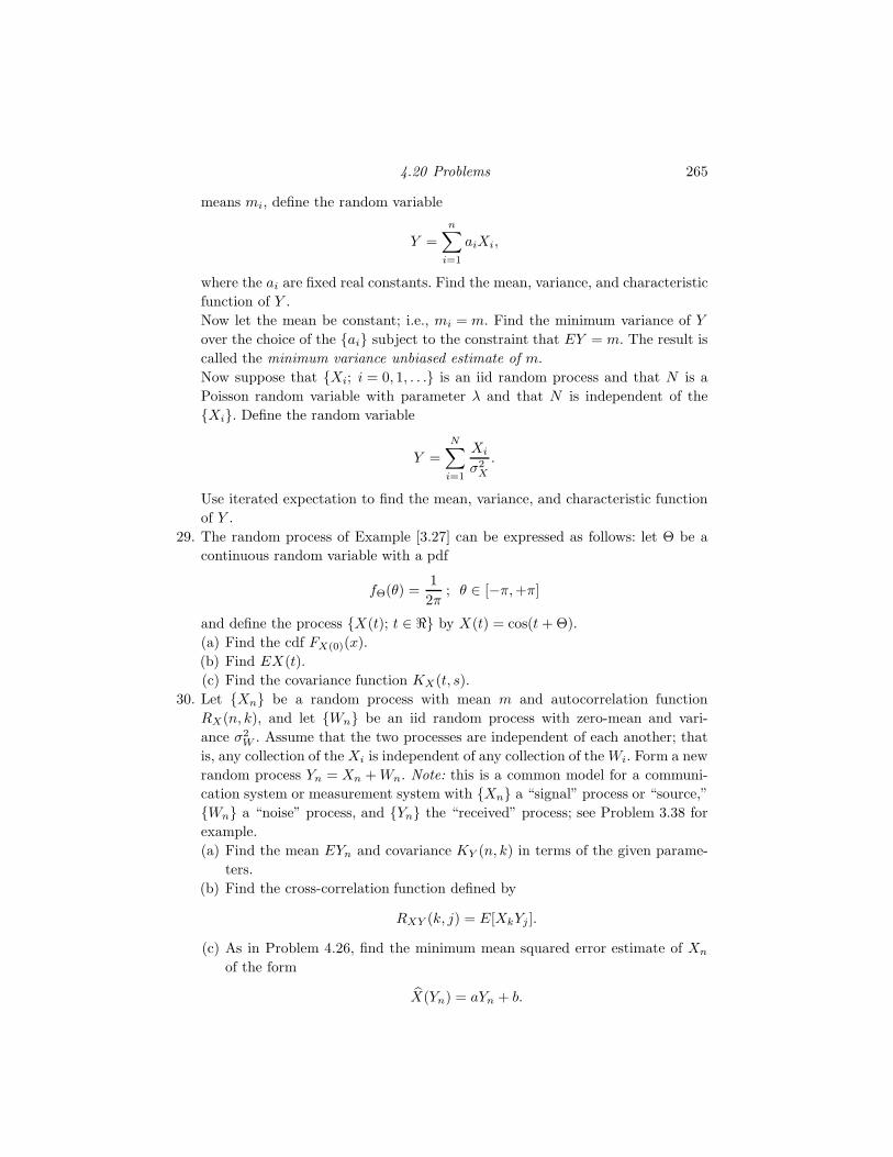
4.20 Problems 265

means mi, define the random variable

Y =n∑

i=1

aiXi,

where the ai are fixed real constants. Find the mean, variance, and characteristic

function of Y .

Now let the mean be constant; i.e., mi = m. Find the minimum variance of Y

over the choice of the ai subject to the constraint that EY = m. The result is

called the minimum variance unbiased estimate of m.

Now suppose that Xi; i = 0, 1, . . . is an iid random process and that N is a

Poisson random variable with parameter λ and that N is independent of the

Xi. Define the random variable

Y =

N∑

i=1

Xi

σ2X

.

Use iterated expectation to find the mean, variance, and characteristic function

of Y .

29. The random process of Example [3.27] can be expressed as follows: let Θ be a

continuous random variable with a pdf

fΘ(θ) =1

2π; θ ∈ [−π, +π]

and define the process X(t); t ∈ ℜ by X(t) = cos(t + Θ).

(a) Find the cdf FX(0)(x).

(b) Find EX(t).

(c) Find the covariance function KX(t, s).

30. Let Xn be a random process with mean m and autocorrelation function

RX(n, k), and let Wn be an iid random process with zero-mean and vari-

ance σ2W . Assume that the two processes are independent of each another; that

is, any collection of the Xi is independent of any collection of the Wi. Form a new

random process Yn = Xn + Wn. Note: this is a common model for a communi-

cation system or measurement system with Xn a “signal” process or “source,”

Wn a “noise” process, and Yn the “received” process; see Problem 3.38 for

example.

(a) Find the mean EYn and covariance KY (n, k) in terms of the given parame-

ters.

(b) Find the cross-correlation function defined by

RXY (k, j) = E[XkYj ].

(c) As in Problem 4.26, find the minimum mean squared error estimate of Xn

of the form

X(Yn) = aYn + b.

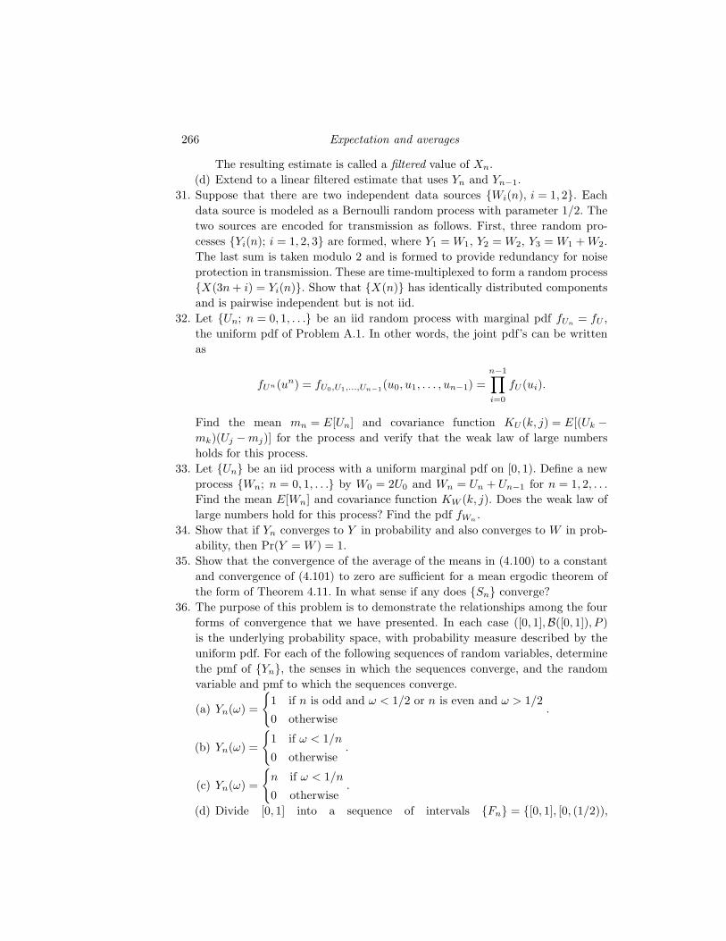
266 Expectation and averages

The resulting estimate is called a filtered value of Xn.

(d) Extend to a linear filtered estimate that uses Yn and Yn−1.

31. Suppose that there are two independent data sources Wi(n), i = 1, 2. Each

data source is modeled as a Bernoulli random process with parameter 1/2. The

two sources are encoded for transmission as follows. First, three random pro-

cesses Yi(n); i = 1, 2, 3 are formed, where Y1 = W1, Y2 = W2, Y3 = W1 + W2.

The last sum is taken modulo 2 and is formed to provide redundancy for noise

protection in transmission. These are time-multiplexed to form a random process

X(3n + i) = Yi(n). Show that X(n) has identically distributed components

and is pairwise independent but is not iid.

32. Let Un; n = 0, 1, . . . be an iid random process with marginal pdf fUn= fU ,

the uniform pdf of Problem A.1. In other words, the joint pdf’s can be written

as

fUn(un) = fU0,U1,...,Un−1(u0, u1, . . . , un−1) =

n−1∏

i=0

fU (ui).

Find the mean mn = E[Un] and covariance function KU (k, j) = E[(Uk −mk)(Uj − mj)] for the process and verify that the weak law of large numbers

holds for this process.

33. Let Un be an iid process with a uniform marginal pdf on [0, 1). Define a new

process Wn; n = 0, 1, . . . by W0 = 2U0 and Wn = Un + Un−1 for n = 1, 2, . . .

Find the mean E[Wn] and covariance function KW (k, j). Does the weak law of

large numbers hold for this process? Find the pdf fWn.

34. Show that if Yn converges to Y in probability and also converges to W in prob-

ability, then Pr(Y = W ) = 1.

35. Show that the convergence of the average of the means in (4.100) to a constant

and convergence of (4.101) to zero are sufficient for a mean ergodic theorem of

the form of Theorem 4.11. In what sense if any does Sn converge?

36. The purpose of this problem is to demonstrate the relationships among the four

forms of convergence that we have presented. In each case ([0, 1],B([0, 1]), P )

is the underlying probability space, with probability measure described by the

uniform pdf. For each of the following sequences of random variables, determine

the pmf of Yn, the senses in which the sequences converge, and the random

variable and pmf to which the sequences converge.

(a) Yn(ω) =

1 if n is odd and ω < 1/2 or n is even and ω > 1/2

0 otherwise.

(b) Yn(ω) =

1 if ω < 1/n

0 otherwise.

(c) Yn(ω) =

n if ω < 1/n

0 otherwise.

(d) Divide [0, 1] into a sequence of intervals Fn = [0, 1], [0, (1/2)),

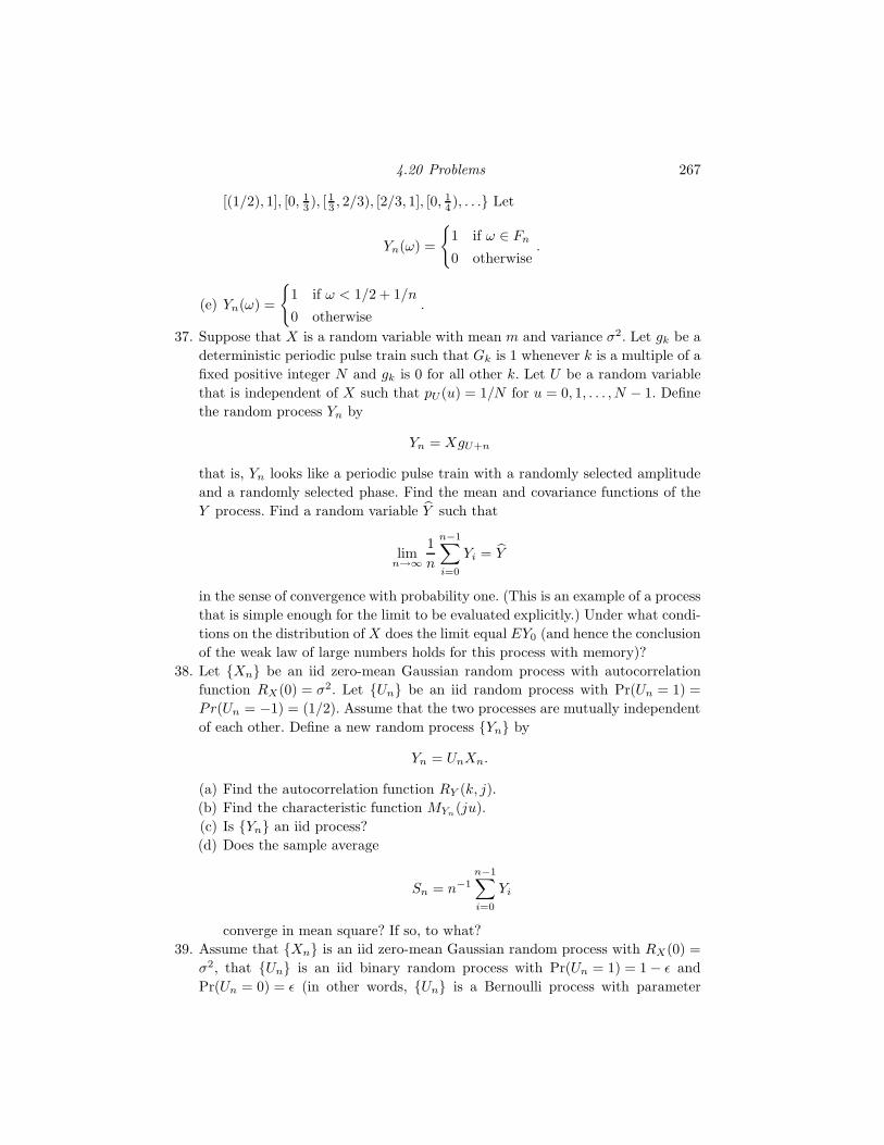
4.20 Problems 267

[(1/2), 1], [0, 13 ), [ 13 , 2/3), [2/3, 1], [0, 1

4 ), . . . Let

Yn(ω) =

1 if ω ∈ Fn

0 otherwise.

(e) Yn(ω) =

1 if ω < 1/2 + 1/n

0 otherwise.

37. Suppose that X is a random variable with mean m and variance σ2. Let gk be a

deterministic periodic pulse train such that Gk is 1 whenever k is a multiple of a

fixed positive integer N and gk is 0 for all other k. Let U be a random variable

that is independent of X such that pU (u) = 1/N for u = 0, 1, . . . , N − 1. Define

the random process Yn by

Yn = XgU+n

that is, Yn looks like a periodic pulse train with a randomly selected amplitude

and a randomly selected phase. Find the mean and covariance functions of the

Y process. Find a random variable Y such that

limn→∞

1

n

n−1∑

i=0

Yi = Y

in the sense of convergence with probability one. (This is an example of a process

that is simple enough for the limit to be evaluated explicitly.) Under what condi-

tions on the distribution of X does the limit equal EY0 (and hence the conclusion

of the weak law of large numbers holds for this process with memory)?

38. Let Xn be an iid zero-mean Gaussian random process with autocorrelation

function RX(0) = σ2. Let Un be an iid random process with Pr(Un = 1) =

Pr(Un = −1) = (1/2). Assume that the two processes are mutually independent

of each other. Define a new random process Yn by

Yn = UnXn.

(a) Find the autocorrelation function RY (k, j).

(b) Find the characteristic function MYn(ju).

(c) Is Yn an iid process?

(d) Does the sample average

Sn = n−1n−1∑

i=0

Yi

converge in mean square? If so, to what?

39. Assume that Xn is an iid zero-mean Gaussian random process with RX(0) =

σ2, that Un is an iid binary random process with Pr(Un = 1) = 1 − ǫ and

Pr(Un = 0) = ǫ (in other words, Un is a Bernoulli process with parameter

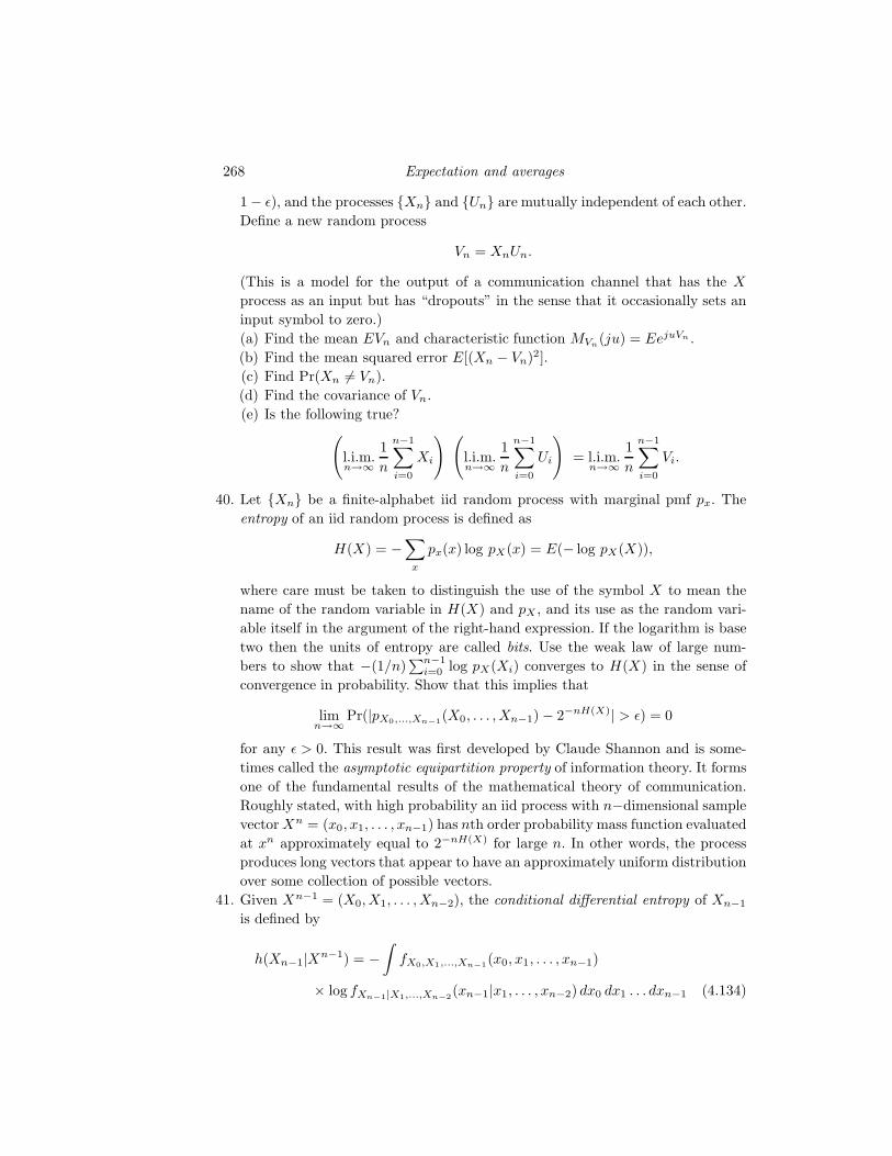
268 Expectation and averages

1 − ǫ), and the processes Xn and Un are mutually independent of each other.

Define a new random process

Vn = XnUn.

(This is a model for the output of a communication channel that has the X

process as an input but has “dropouts” in the sense that it occasionally sets an

input symbol to zero.)

(a) Find the mean EVn and characteristic function MVn(ju) = EejuVn .

(b) Find the mean squared error E[(Xn − Vn)2].

(c) Find Pr(Xn 6= Vn).

(d) Find the covariance of Vn.

(e) Is the following true?(

l.i.m.n→∞

1

n

n−1∑

i=0

Xi

) (l.i.m.n→∞

1

n

n−1∑

i=0

Ui

)= l.i.m.

n→∞1

n

n−1∑

i=0

Vi.

40. Let Xn be a finite-alphabet iid random process with marginal pmf px. The

entropy of an iid random process is defined as

H(X) = −∑

x

px(x) log pX(x) = E(− log pX(X)),

where care must be taken to distinguish the use of the symbol X to mean the

name of the random variable in H(X) and pX , and its use as the random vari-

able itself in the argument of the right-hand expression. If the logarithm is base

two then the units of entropy are called bits. Use the weak law of large num-

bers to show that −(1/n)∑n−1

i=0 log pX(Xi) converges to H(X) in the sense of

convergence in probability. Show that this implies that

limn→∞

Pr(|pX0,...,Xn−1(X0, . . . , Xn−1) − 2−nH(X)| > ǫ) = 0

for any ǫ > 0. This result was first developed by Claude Shannon and is some-

times called the asymptotic equipartition property of information theory. It forms

one of the fundamental results of the mathematical theory of communication.

Roughly stated, with high probability an iid process with n−dimensional sample

vector Xn = (x0, x1, . . . , xn−1) has nth order probability mass function evaluated

at xn approximately equal to 2−nH(X) for large n. In other words, the process

produces long vectors that appear to have an approximately uniform distribution

over some collection of possible vectors.

41. Given Xn−1 = (X0, X1, . . . , Xn−2), the conditional differential entropy of Xn−1

is defined by

h(Xn−1|Xn−1) = −∫

fX0,X1,...,Xn−1(x0, x1, . . . , xn−1)

× log fXn−1|X1,...,Xn−2(xn−1|x1, . . . , xn−2) dx0 dx1 . . . dxn−1 (4.134)

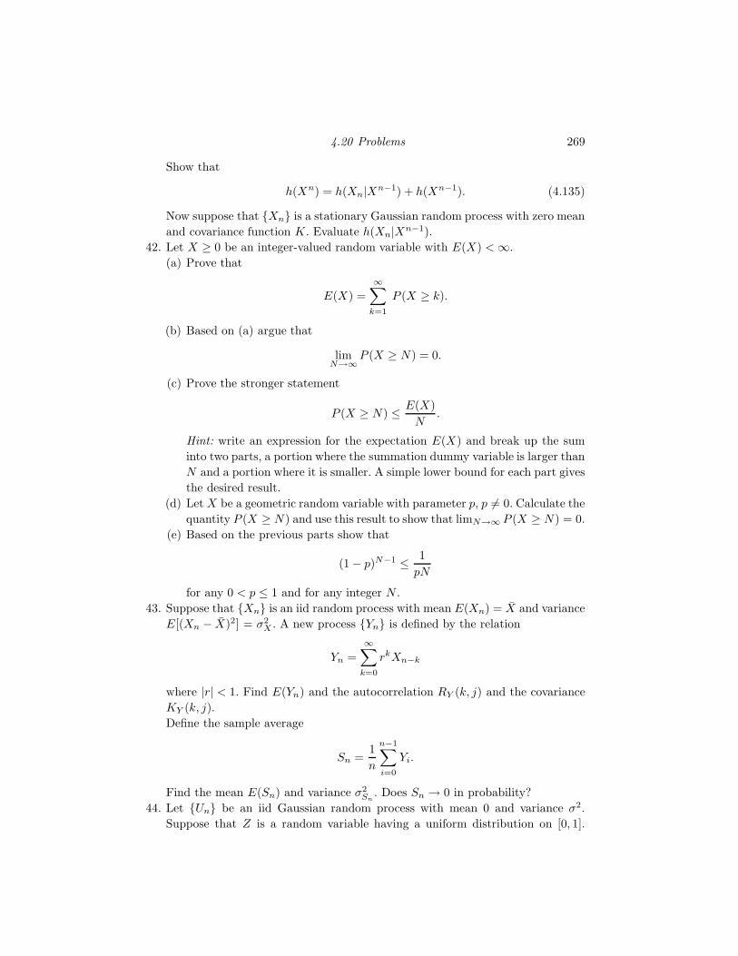
4.20 Problems 269

Show that

h(Xn) = h(Xn|Xn−1) + h(Xn−1). (4.135)

Now suppose that Xn is a stationary Gaussian random process with zero mean

and covariance function K. Evaluate h(Xn|Xn−1).

42. Let X ≥ 0 be an integer-valued random variable with E(X) < ∞.

(a) Prove that

E(X) =

∞∑

k=1

P (X ≥ k).

(b) Based on (a) argue that

limN→∞

P (X ≥ N) = 0.

(c) Prove the stronger statement

P (X ≥ N) ≤ E(X)

N.

Hint: write an expression for the expectation E(X) and break up the sum

into two parts, a portion where the summation dummy variable is larger than

N and a portion where it is smaller. A simple lower bound for each part gives

the desired result.

(d) Let X be a geometric random variable with parameter p, p 6= 0. Calculate the

quantity P (X ≥ N) and use this result to show that limN→∞ P (X ≥ N) = 0.

(e) Based on the previous parts show that

(1 − p)N−1 ≤ 1

pN

for any 0 < p ≤ 1 and for any integer N .

43. Suppose that Xn is an iid random process with mean E(Xn) = X and variance

E[(Xn − X)2] = σ2X . A new process Yn is defined by the relation

Yn =

∞∑

k=0

rkXn−k

where |r| < 1. Find E(Yn) and the autocorrelation RY (k, j) and the covariance

KY (k, j).

Define the sample average

Sn =1

n

n−1∑

i=0

Yi.

Find the mean E(Sn) and variance σ2Sn

. Does Sn → 0 in probability?

44. Let Un be an iid Gaussian random process with mean 0 and variance σ2.

Suppose that Z is a random variable having a uniform distribution on [0, 1].

270 Expectation and averages

Suppose Z represents the value of a measurement taken by a remote sensor and

that we wish to guess the value of Z based on a noisy sequence of measurements

Yn = Z + Un, n = 0, 1, 2, . . .; that is, we observe only Yn and wish to estimate

the underlying value of Z. To do this we form a sample average and define the

estimate

ZN =1

N

n−1∑

i=0

Yi.

(a) Find a simple upper bound to the probability

Pr(|Zn − Z| > ǫ)

that goes to zero as n → ∞. (This means that our estimator is asymptoti-

cally good.)

Suppose next that we have a two-dimensional random process Un, Wn (i.e.,

the output at each time is a random pair or a two-dimensional random vari-

able) with the following properties. Each pair (Un, Wn) is independent of all

past and future pairs (Uk, Wk) k 6= n. Each pair (Un, Wn) has an identical

joint cdf FU,W (u, w). For each n E[Un] = E[Wn] = 0, E[U2n] = E[W 2

n ] = σ2, and

E[UnWn] = ρσ2. (The quantity ρ is called the correlation coefficient.) Instead of

just observing a noisy sequence Yn = Z + Un, we also observe a separate noisy

measurement sequence Xn = Z + Wn (the same Z, but different noises). Sup-

pose further that we try to improve our estimate of Z by using both of these

measurements to form an estimate

Z = a1

n

n−1∑

i=0

Yi + (1 − a)1

n

n−1∑

i=0

Xi.

for some a in [0, 1].

(a) Show that |ρ| ≤ 1. Find a simple upper bound to the probability

Pr(|Zn − Z| > ǫ)

that goes to zero as n → ∞. What value of a gives the smallest upper bound

in part (b) and what is the resulting bound? (Note as a check that the bound

should be no worse than part (a) since the estimator of part (a) is a special

case of that of part (b).) In the special case where ρ = −1, what is the best

a and what is the resulting bound?

45. Suppose that Xn are iid random variables described by a common marginal

distribution F . Suppose that the random variables

Sn =1

n

n−1∑

i=0

Xi

4.20 Problems 271

also have the distribution F for all positive integers n. Find the form of the dis-

tribution F . (This is an example of what is called a stable distribution.) Suppose

that the 1/n in the definition of Sn is replaced by 1/√

n. What must F then be?

46. Consider the following nonlinear modulation scheme: define

W (t) = ej(2πf0t+cX(t)+Θ),

X(t) is a zero-mean weakly stationary Gaussian random process with autocor-

relation function RX(τ), f0 is a fixed frequency, Θ is a uniform random variable

on [0, 2π], Θ is independent of all of the X(t), and c is a modulation constant.

(This is a mathematical model for phase modulation.)

Define the expectation of a complex random variable in the natural way: if Z =

ℜ(Z) + jℑ(Z), then E(Z) = E[ℜ(Z)] + jE[ℑ(Z)].) Define the autocorrelation of

a complex -valued random process W (t) by

RW (t, s) = E(W (t)W (s)∗),

where W (s)∗ denotes the complex conjugate of W (s).

Find the mean E(W (t)) and the autocorrelation function RW (t, s) =

E[W (t)W (s)∗].Hint: the autocorrelation is admittedly a trick question (but a very useful trick).

Keep characteristic functions in mind when pondering the evaluation of the au-

tocorrelation function.

47. Suppose that Xn; n = 0, 1, . . . is a discrete time iid random process with pmf

pXn(k) = (1/2); k = 0, 1.

Two other random processes are defined in terms of the X process:

Yn =

n∑

i=0

Xi; n = 0, . . .

Wn = (−1)Yn n = 0, 1, . . .

and

Vn = Xn − Xn−1; n = 1, . . .

(a) Find the covariance functions for the X and Y processes.

(b) Find the mean and variance of the random variable Wn. Find the covariance

function of the process Wn.

(c) Find the characteristic function of the random variable Vn.

(d) Which of the above four processes are weakly stationary? Which are not?

(e) Evaluate the limits l.i.m.n→∞Yn

n+1 , l.i.m.n→∞Yn

n2 and l.i.m.n→∞1n

∑nl=1 Vl.

(f) For the showoffs: does the last limit above converge with probability one?

(Only elementary arguments are needed.)

272 Expectation and averages

48. Suppose that Xn is a discrete time iid random process with uniform marginal

pdf’s

fXn(α) =

1 0 ≤ α < 1

0 otherwise.

Define the following random variables:

• U = X20

• V = max(X1, X2, X3, X4)

• W =

1 if X1 ≥ 2X2

0 otherwise.

• For each integer n Yn = Xn + Xn−1. Note that this defines a new random

process Yn.(a) Find the expected values of the random variables U , V , and W .

(b) What are the mean E(Xn) and covariance function KX(k, j) of Xn?(c) What are the mean E(Yn) and covariance function KY (k, j) of Yn?(d) Define the sample average

Sn =1

n

n∑

k=1

Yk.

Find the mean E(Sn) and variance σ2Sn

of Sn. Using only these results (and

no results not yet covered), find l.i.m.n→∞Sn.

(e) Does the sequence of random variables

Zn =

n∏

i=1

Xi

converge in probability to 0?

49. A discrete time martingale Yn; n = 0, 1, . . . is a process with the property that

E[Yn|Y0, Y1, . . . , Yn−1] = Yn.

In words, the conditional expectation of the current value is the previous value.

Suppose that Xn is iid. Is

Yn =n−1∑

n=0

Xn

a martingale?

50. Let Yn be the one-dimensional random walk of Chapter 3.

(a) Find the pmf pYnfor n = 0, 1, 2.

(b) Find the mean E[Yn] and variance σ2Yn

.

(c) Does Yn/n converge as n gets large?

(d) Find the conditional pmf’s pYn|Y0,Y1,...,Yn−1(yn|y0, y1, . . . , yn−1) and

pYn|Yn−1(yn|yn−1). Is this process Markov?

4.20 Problems 273

(e) What is the minimum MSE estimate of Yn given Yn−1? What is the proba-

bility that Yn actually equals its minimum MSE estimate?

51. Let Xn be a binary iid process with pX(±1) = 0.5. Define a new process

Wn; n = 0, 1, . . . by

Wn = Xn + Xn−1.

This is an example of a moving-average process, so called because it computes a

short term average of the input process. Find the mean, variance, and covariance

function of Wn. Prove a weak law of large numbers for Wn.

52. How does one generate a random process? It is often of interest to do so in order

to simulate a physical system in order to test an algorithm before it is applied

to genuine data. Using genuine physical data may be too expensive, dangerous,

or politically risky. One might connect a sensor to a resistor and heat it up to

produce thermal noise, or flip a coin a few million times. One solution requires

uncommon hardware and the other physical effort. The usual solution is to use

a computer to generate a sequence that is not actually random, but pseudo-

random in that it can produce a long sequence of numbers that appear to be

random and will satisfy several tests for randomness, provided that the tests

are not too stringent. An example is the rand command used in MatlabTM. It

uses the linear congruential method which starts with a “seed” X0 and then

recursively defines the sequence

Xn = (77Xn−1) mod (231 − 1). (4.136)

This produces a sequence of integers in the range from 0 to 231 − 1. Dividing by

231 (which is just a question of shifting in binary arithmetic) produces a number

in the range [0, 1). Find a computer with Matlab or program this algorithm

yourself and try it out with different starting sequences. Find the sample average

Sn of a sequence of 100, 1000, and 10,000 samples and compare them to the

expected value of the uniform pdf random variable considered in this chapter.

How might you determine whether or not the sequence being viewed was indeed

random or not if you did not know how it was generated?

53. Suppose that U is a random variable with pdf fU (u) = 1 for u ∈ [0, 1). Describe a

function q : [0, 1) → A, where A = 0, 1, . . . , K − 1, so that the random variable

X = q(U) is discrete with pmf

pX(k) =1

K; k = 0, 1, . . . , K − 1.

You have produced a uniform discrete random variable from a uniform continuous

random variable.

(a) What is the minimum mean squared error estimator of U given X = k? Call

this estimator U(k). Write an expression for the resulting MSE

E[(U − U(q(U))]2.

274 Expectation and averages

(b) Show that the estimator U found in the previous part minimizes the MSE

E[(U − U(q(U))2] between the original input and the final output (assuming

that q is fixed). You have just demonstrated one of the key properties of a

Lloyd–Max quantizer (see, e.g., [26]).

(c) Find the pmf for the random variable U = U(q(U)). Find E[U ] and σ2U

. How

do the mean and variance of the U compare with those of U? (equal, bigger,

smaller?)

54. Modify the development in the text for the minimum mean squared error estima-

tor to work for discrete random variables. What is the minimum MSE estimator

for Yn given Yn−1 for the binary Markov process developed in the chapter?

Which do you think makes more sense for guessing the next outcome for a bi-

nary Markov process, the minimum probability of error classifier or the minimum

MSE estimator? Explain.

55. Let Yn; n = 0, 1, . . . be the binary Markov process developed in the chapter.

Find a new process Wn; n = 1, 2, . . . defined by Wn = Yn ⊕ Yn−1. Describe the

process Wn.

Problems 56–62 courtesy of the EE Department of the Technion.

56. Let X be a Gaussian random variable with zero-mean and variance σ2.

(a) Find E[cos(nX)], n = 1, 2, . . .

(b) Find E[Xn], n = 1, 2, . . .

(c) Let N be a Poisson random variable with parameter λ and assume that X

and N are independent. Find E[Xn].

Hint: use characteristic functions and iterated expectation.

57. Let X be a random variable with uniform pdf on [−1, 1]. Define a new random

variable Y by

Y =

X X ≤ 0

1 X > 0.

(a) Find the cdf FY (y) and plot it.

(b) Find the pdf fY (y).

(c) Find E(Y ) and σ2Y .

(d) Find E(X |Y ).

(e) Find E[(X − E(X |Y ))2].

58. Let X1, X2, . . . , Xn be zero-mean statistically independent random variables.

Define

Yn =

n∑

i=1

Xi.

Find E(Y7|Y1, Y2, Y3).

59. Let U denote a binary random variable with pmf pU (u) = 0.5 for u = ±1. Let

4.20 Problems 275

Y = U + X , where X is N (0, σ2) and where U and X are independent. Find

E(U |Y ).

60. Let Y, N1, N2 be zero-mean, unit-variance, mutually independent random vari-

ables. Define

X1 = Y + N1 +√

αN1

X2 = Y + 3N1 +√

αN1.

(a) Find the linear MMSE estimator of Y given X1 and X2.

(b) Find the resulting MSE.

(c) For what value of α ∈ [0,∞) does the mean squared error become zero?

Provide an intuitive explanation.

61. Let Xn; n = 1, 2, . . . be an iid sequence of N (m, σ2) random variables. Define

for any positive integer N

SN =N∑

n=1

Xn.

(a) For K < N find the pdf fSN |SK(α|β).

(b) Find the MMSE estimator of SK given SN , E(SK |SN ). Define VK =∑Kn=1 X2

n. Find the linear MMSE of VK given VN .

62. Let Xi = S + Wi, i = 1, 2, . . . , N , where S and the Wi are mutually independent

with zero-mean. The variance of S is σS and the variances of all the Wi are σ2W .

(a) Find the linear MMSE of S given the observations Xi, i = 1, 2, . . . , N .

(b) Find the resulting MSE.

63. Suppose that Xn; n = 0, 1, . . . is a Gaussian iid process with zero-mean and

variance σ2X . Let Yn; n = 0, 1, 2, . . . be an iid Bernoulli process with parameter

p. Define the random variables

Sn =1

n

n−1∑

i=0

Xi; n = 1, 2, 3, . . .

and

Nn =

n−1∑

i=0

Yi; n = 1, 2, 3, . . .

(a) Find the mean, variance, transform, and pdf for Sn.

(b) Find the mean, variance, transform, and pmf for Nn.

(c) Find the mean, variance, and transform for SNn.

(d) Does Sn converge in mean square as n → ∞? If so, to what?

(e) Does SNnconverge in probability as n → ∞? If so, to what?

5

Second-order theory

In Chapter 4 we saw that the second-order moments of a random process

– the mean and covariance or, equivalently, the autocorrelation – play a

fundamental role in describing the relation of limiting sample averages and

expectations. We also saw, for example in Section 4.6.1 and Problem 4.26,

that these moments also play a key role in signal processing applications

of random processes, especially in linear least squares estimation. Because

of the fundamental importance of these particular moments, this chapter

considers their properties in greater depth and their evaluation for several

important examples. A primary focus is on a second-order moment analog

of a derived distribution problem. Suppose we are given the second-order

moments of one random process and this process is then used as an input

to a linear system. What are the resulting second-order moments of the

output random process? These results are collectively known as second-order

moment input/output or I/O relations for linear systems.

Linear systems may seem to be a very special case. As we will see, their

most obvious attribute is that they are easier to handle analytically, which

leads to more complete, useful, and stronger results than can be obtained for

the class of all systems. This special case, however, plays a central role and is

by far the most important class of systems. The design of engineering systems

frequently involves the determination of an optimum system – perhaps the

optimum signal detector for a signal in noise, the filter that provides the

highest signal-to-noise ratio, the optimum receiver, etc. Surprisingly enough,

the optimum is frequently a linear system. Even when it is not, often a

linear system is a good enough approximation to be used for the sake of

economical design. For these reasons it is of interest to study the properties

of the output random process from a linear system that is driven by a

specified input random process. In this chapter we consider only second-

order moments. In the next chapter we consider examples in which one can

276

5.1 Linear filtering of random processes 277

develop a more complete probabilistic description of the output process. As

one might suspect the less complete second-order descriptions are possible

under far more general conditions.

When a linear system is driven by a given random process, the second-

order properties of the output process provide the fundamental tools for

analysis and optimization. As an example of such analysis, the chapter closes

with an application of second-order moment theory to the design of systems

for linear least squares estimation.

Because the primary engineering application of these systems is to noise

discrimination, we will group them together under the name “linear filters.”

This designation denotes the suppression or “filtering out” of noise from the

combination of signal and noise. The methods of analysis are not limited to

this application, of course.

As usual, we emphasize discrete time in the development, with the obvi-

ous extensions to continuous time provided by integrals. Furthermore, we

restrict attention in the basic development to linear time-invariant filters.

The extension to time-varying systems is obvious but cluttered with ob-

fuscating notation. Time-varying systems will be encountered briefly when

considering recursive estimation.

We initially follow a somewhat cavalier attitude in terms of how infinite

sums and integrals are defined for random processes. We subsequently ex-

plore the use of second-order moments to provide rigorous definitions of

these ideas using mean square convergence of random variables. This pro-

vides a more careful treatment of integrals and hence also of linear filtering

and linear operations such as differentiation and integration of continuous

time random processes.

5.1 Linear filtering of random processes

Suppose that a random process X(t); t ∈ T (or Xt; t ∈ T ) is used as

an input to a linear time-invariant system described by a δ-response h.

Hence the output process, say Y (t) or Yt is described by the convolution

integral (A.35) in the continuous time case and by the convolution sum

(A.42) in the discrete time case. To be precise, we have to be careful about

how the integral or sum is defined; integrals and infinite sums of random

processes are really limits of random variables, and those limits can converge

in a variety of ways, such as in quadratic mean or with probability one. For

the moment we will assume that the convergence is with probability one,

i.e., that each realization or sample function of the output is related to the

278 Second-order theory

corresponding realization of the input via (A.35) or (A.42). That is, we take

Y (t) =

∫

s: t−s∈TX(t − s)h(s) ds (5.1)

or

Yn =∑

k:n−k∈TXn−khk (5.2)

to mean actual equality for a collection of elementary events ω on the under-

lying probability space Ω collectively having probability one. More precisely,

with probability one

Y (t, ω) =

∫

s: t−s∈TX(t − s, ω)h(s) ds

or

Yn(ω) =∑

k:n−k∈TXn−k(ω)hk,

respectively. As has been discussed earlier, it can be extremely difficult to

demonstrate that such forms of convergence actually hold for a particular

random process and δ-response, but the results obtained by such formal

manipulations can be demonstrated rigorously under suitable technical as-

sumptions either through advanced mathematical methods (which are not

considered here) or by using weaker notions of convergence of random vari-

ables – in particular by using mean square convergence to define both infinite

sums and integrals (which we will do later in this chapter).

Rigorous consideration of conditions under which the various limits exist

is straightforward for the discrete time case. It is obvious that the limits exist

for the so-called finite impulse response (FIR) discrete time filters where

only a finite number of the hk are nonzero and hence the sum has only a

finite number of terms. It is also possible to show mean square convergence

for the general discrete time convolution if the input process has finite mean

and variance and if the filter is stable in the sense of (A.43). In particular,

for a one-sided input process, (5.2) converges in quadratic mean; i.e.,

l.i.m.n→∞

n−1∑

k=0

Xn−khk

converges. Initially we ignore these technical difficulties and just assume that

the sums and integrals are well defined.

Fourier analysis plays a fundamental role in the study of linear systems,

but unfortunately (A.37) and (A.43) are not satisfied in general for sample

5.2 Linear systems I/O relations 279

functions of interesting random processes and hence one cannot simply take

Fourier transforms of both sides of (5.1) and (5.2) and obtain a useful spec-

tral relation. Even if one could, the Fourier transform of a random process

would be a random variable for each value of frequency! Because of this,

the frequency domain theory for random processes is quite different from

that for deterministic processes. Relations such as (A.39) may on occasion

be useful for intuition, but they must be used with extreme care.

With the foregoing notation and preliminary considerations, we now turn

to the analysis of discrete time linear filters with random process inputs.

5.2 Linear systems I/O relations

Discrete time systems

Ideally one would like to have a complete specification of the output of

a linear system as a function of the specification of the input random pro-

cess. Usually this is a difficult proposition because of the complexity of the

computations required. However, it is a relatively easy task to determine the

mean and covariance function at the output. As we will show, the output

mean and covariance function depend only on the input mean and covariance

function and on no other properties of the input random process. Further-

more, in many, if not most, applications, the mean and covariance functions

of the output are all that are needed to solve the problem at hand. As an

important example: if the random process is Gaussian, then the mean and

covariance functions provide a complete description of the process.

Linear filter input/output (I/O) relations are most easily developed using

the convolution representation of a linear system. Let Xn be a discrete

time random process with mean function mn = EXn and covariance function

KX(n, k) = E[(Xn − mn)(Xk − mk)]. Let hk be the Kronecker δ-response

of a discrete time linear filter. For notational convenience we assume that

the δ-response is causal. The noncausal case simply involves a change of the

limits of summation. Next we will find the mean and covariance functions for

the output process Yn that is given in the convolution equation of (5.2).

From (5.2) the mean of the output process is found using the linearity of

expectation as

EYn =∑

k

hkEXn−k =∑

k

hkmn−k, (5.3)

assuming, of course, that the sum exists. The sum does exist if the filter

is stable and the input mean is bounded. That is, if there is a constant

280 Second-order theory

m < ∞, such that |mn| ≤ |m| for all n and if the filter is stable in the sense

of equation (A.43), then

|EYn| =

∣∣∣∣∣∑

k

hkmm−k

∣∣∣∣∣ ≤ maxk

|mn−k|∑

k

|hk| ≤ |m|∑

k

|hk| < ∞.

If the input process Xn is weakly stationary, then the input mean function

equals the constant, m, and

EYn = m∑

k

hk, (5.4)

which is the dc response of the filter times the mean. For reference we specify

the precise limits for the two-sided random process where T = Z and for the

one-sided input random process where T = Z+:

EYn = m

∞∑

k=0

hk, T = Z (5.5)

EYn = m

n∑

k=0

hk, T = Z+. (5.6)

Thus, if the input random process is weakly stationary, then the output

mean exists if the input mean is finite and the filter is stable. In addition,

it can be seen that for two-sided weakly stationary random processes, the

expected value of the output process does not depend on the time index n

since the limits of the summation do not depend on n. For one-sided weakly

stationary random processes, however, the output mean is not constant with

time but approaches a constant value as n → ∞ if the filter is stable. Note

that this means that if a one-sided stationary process is put into a linear

filter, the output is in general not stationary!

If the filter is not stable, the magnitude of the output mean is unbounded

with time. For example, if we set hk = 1 for all k in (5.6) then EYn =

(n + 1)m, which very strongly depends on the time index n and which is

unbounded.

Turning to the calculation of the output covariance function, we use equa-

5.2 Linear systems I/O relations 281

tions (5.2) and (5.3) to evaluate the covariance with some bookkeeping as

KY (k, j) = E[(Yk − EYk)(Yj − EYj)]

= E

[(∑

n

hn(Xk−n − mk−n)

)(∑

m

hm(Xj−m − mj−m)

)]

=∑

n

∑

m

hnhmE[(Xk−n − mk−n)(Xj−m − mj−m)]

=∑

n

∑

m

hnhmKX(k − n, j − m). (5.7)

A careful reader might note the similarity between (5.7) and the correspond-

ing matrix equation (4.28) derived during the consideration of Gaussian vec-

tors (but true generally for covariance matrices of linear functions of random

vectors).

As before, the range of the sums depends on the index set used. Since

we have specified causal filters, the sums run from 0 to ∞ for two-sided

processes and from 0 to k and 0 to j for one-sided random processes.

It can be shown that the sum of (5.7) converges if the filter is stable in

the sense of (A.43) and if the input process has bounded variance; i.e., there

is a constant σ2 < ∞ such that |KX(n, n)| < σ2 for all n (Problem 5.19).

If the input process is weakly stationary, then KX depends only on the

difference of its arguments. This is made explicit by replacing KX(m,n) by

KX(m − n). Then (5.7) becomes

KY (k, j) =∑

n

∑

m

hnhmKX((k − j) − (n − m)). (5.8)

Specifying the limits of the summation for the one-sided and two-sided cases,

we have that

KY (k, j) =

∞∑

n=0

∞∑

m=0

hnhmKX((k − j) − (n − m)) ; T = Z. (5.9)

and

KY (k, j) =k∑

n=0

j∑

m=0

hnhmKX((k − j) − (n − m)) ; T = Z+. (5.10)

If the sum of (5.9) converges (e.g., if the filter is stable and KX(n, n) =

KX(0) < ∞), then two interesting facts follow. First, if the input random

process is weakly stationary and if the processes are two-sided, then the

covariance of the output process depends only on the time lag; i.e., KY (k, j)

can be replaced by KY (k − j). Note that this is not the case for a one-sided

282 Second-order theory

process, even if the input process is stationary and the filter stable! This fact,

together with our earlier result regarding the mean, can be summarized as

follows.

Given a two-sided random process as input to a linear filter, if the input

process is weakly stationary and the filter is stable, the output random

process is also weakly stationary. The output mean and covariance functions

are given by

EYn = m

∞∑

k=0

hk (5.11)

KY (k) =∞∑

n=0

∞∑

m=0

hnhmKX(k − (n − m)). (5.12)

The second observation is that (5.8), (5.9), (5.10) or (5.12) is a double

discrete convolution! The direct evaluation of (5.8), (5.9), and (5.10), while

straightforward in concept, can be an exceedingly involved computation in

practice. As in other linear systems applications, the evaluations of convo-

lutions can often be greatly simplified by resort to transform techniques, as

be considered shortly.

Continuous time systems

For each of the discrete time filter results there is an analogous continuous

time result. For simplicity, however, we consider only the simpler case of two-

sided processes. Let X(t) be a two-sided continuous time input random

process to a linear time-invariant filter with impulse response h(t).

We can evaluate the mean and covariance functions of the output process

in terms of the mean and covariance functions of the input random process by

using the same development as was used for discrete time random processes.

This time we have integrals instead of sums. Let m(t) and KX(t, s) be the

respective mean and covariance functions of the input process. Then the

mean function of the output process is

EY (t) =

∫E[X(t − s)]h(s) ds =

∫m(t − s)h(s) ds. (5.13)

The covariance function of the output random process is obtained by com-

putations analogous to (5.7) as

KY (t, s) =

∫dα

∫dβKX(t − α, s − β)h(α)h(β). (5.14)

5.2 Linear systems I/O relations 283

Thus if X(t) is weakly stationary with mean m = m(t) and covariance

function KX(τ), then

EY (t) = m

∫h(t) dt (5.15)

and

KY (t, s) =

∫dα

∫dβKX((t − s) − (α − β))h(α)h(β). (5.16)

In analogy to the discrete time result, the output mean is constant for a

two-sided random process, and the covariance function depends on only the

time difference. Thus a weakly stationary two-sided process into a stable

linear time-invariant filter yields a weakly stationary output process in both

discrete and continuous time. We leave it to the reader to develop conclusions

that are parallel to the discrete time results for one-sided processes.

Transform I/O relations

In both discrete and continuous time, the covariance function of the out-

put can be found by first convolving the input autocorrelation with the

δ-response hk or h(t) and then convolving the result with the reflected δ-

response h−k or h(−t). A way of avoiding the double convolution is found

in Fourier transforms. Taking the Fourier transform (continuous or discrete

time) of the double convolution yields the transform of the covariance func-

tion, which can be used to arrive at the output covariance function – essen-

tially the same result with (in many cases) less overall work.

We shall show the development for discrete time. A similar sequence of

steps provides the proof for continuous time by replacing the sums by inte-

grals. Using (5.12),

Ff (KY )

=∑

k

(∑

n

∑

m

hnhmKX(k − (n − m))

)

e−j2πfk

=∑

n

∑

m

hnhm

(∑

k

KX(k − (n − m))e−j2πf(k−(n−m))

)e−j2πf(n−m)

=

(∑

n

hne−j2πfn

)(∑

m

hme+j2πfm

)F(KX)

= Ff (KX)Ff (h)Ff (h∗), (5.17)

284 Second-order theory

where the asterix denotes complex conjugate. If we define H(f) = Ff (h),

the transfer function of the filter, then the result can be abbreviated for

both continuous and discrete time as

Ff (KY ) = |H(f)|2Ff (KX). (5.18)

We can also conveniently describe the mean and autocorrelation functions

in the frequency domain. From (5.5) and (5.15) the mean mY of the output

is related to the mean mY of the input simply as

mY = H(0)mX . (5.19)

Since KX(k) = RX(k) − |mX |2 and KY (k) = RY (k) − |mY |2, (5.18) implies

that

Ff (RY − |mY |2) = |H(f)|2Ff (RX − |mX |2)

or

Ff (RY ) − |mY |2δ(f) = |H(f)|2(Ff (RX) − |mX |2δ(f)

)

= |H(f)|2Ff (RX) − |H(f)|2|mX |2δ(f)

= |H(f)|2Ff (RX) − |H(0)|2|mX |2δ(f),

where we have used the property of Dirac deltas that g(f)δ(f) = g(0)δ(f)

(provided g(f) has no jumps at f = 0). Thus the autocorrelation function

satisfies the same transform relation as the covariance function. This result is

abbreviated by giving a special notation to the transform of an autocorrela-

tion function: given a weakly stationary process X(t) with autocorrelation

function RX , the power spectral density of the process is defined by

SX(f) = Ff (RX) =

∑kRX(k)e−j2πfk discrete time

∫RX(τ)e−j2πfτ dτ continuous time

, (5.20)

the Fourier transform of the autocorrelation function. The reason for the

name will be given in the next section and discussed at further length later

in the chapter. Given the definition we have now proved the following result.

If a weakly stationary process X(t) with power spectral density SX(f)

is the input to a linear time-invariant filter with transfer function H, then

the output process Y (t) is also weakly stationary and has mean

mY = H(0)mX (5.21)

5.3 Power spectral densities 285

and power spectral density

SY (f) = |H(f)|2SX(f). (5.22)

This result is true for both discrete and continuous time.

5.3 Power spectral densities

Under suitable technical conditions the Fourier transform can be inverted to

obtain the autocorrelation function from the power spectral density. Thus

the reader can verify from the definitions (5.20) that

RX(τ) =

∫ 1/2−1/2

SX(f)ej2πfτ df discrete time∫∞−∞SX(f)ej2πfτ dτ continuous time

. (5.23)

The limits of −1/2 to +1/2 for the discrete time integral correspond to the

fact that time is measured in units; e.g., adjacent outputs are one second or

one minute or one year apart. Sometimes, however, the discrete time process

is formed by sampling a continuous time process at every, say, T seconds,

and it is desired to retain seconds as the unit of measurement. Then it is

more convenient to incorporate the scale factor T into the time units and

scale (5.20) and the limits of (5.23) accordingly – i.e., kT replaces k in (5.20),

and the limits become −1/2T to 1/2T .

Power spectral densities inherit the property of symmetry from auto-

correlation functions. As seen from the definition in Chapter 4, covariance

and autocorrelation functions are symmetric (RX(t, s) = RX(s, t)). There-

fore RX(τ) is an even function. From (5.20) it can be seen with a little

juggling that SX(f) is also even; that is, SX(−f) = SX(f) for all f .

The name “power spectral density” comes from observing how the average

power of a random process is distributed in the frequency domain. The

autocorrelation function evaluated at 0 lag, PX = RX(0) = E(|X(t)|2), can

be interpreted as the average power dissipated in a unit resistor by a voltage

X(t). Since the autocorrelation is the inverse Fourier transform of the power

spectral density, this means that

PX =

∫SX(f) df, (5.24)

that is, the total average power in the process can be found by integrating

SX(f). Thus if SX were nonnegative, it could be considered as a density of

power analogous to integrating a probability or mass density to find total

probability or mass. For the probability and mass analogues, however, we

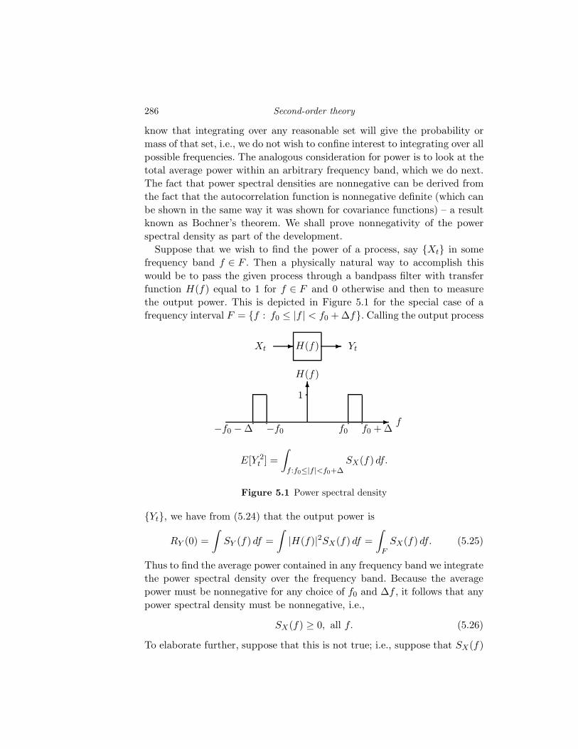
286 Second-order theory

know that integrating over any reasonable set will give the probability or

mass of that set, i.e., we do not wish to confine interest to integrating over all

possible frequencies. The analogous consideration for power is to look at the

total average power within an arbitrary frequency band, which we do next.

The fact that power spectral densities are nonnegative can be derived from

the fact that the autocorrelation function is nonnegative definite (which can

be shown in the same way it was shown for covariance functions) – a result

known as Bochner’s theorem. We shall prove nonnegativity of the power

spectral density as part of the development.

Suppose that we wish to find the power of a process, say Xt in some

frequency band f ∈ F . Then a physically natural way to accomplish this

would be to pass the given process through a bandpass filter with transfer

function H(f) equal to 1 for f ∈ F and 0 otherwise and then to measure

the output power. This is depicted in Figure 5.1 for the special case of a

frequency interval F = f : f0 ≤ |f | < f0 + ∆f. Calling the output process

Xt- H(f) - Yt

- f

6H(f)

1

−f0 − ∆ −f0 f0 f0 + ∆

E[Y 2t ] =

∫

f :f0≤|f |<f0+∆SX(f) df.

Figure 5.1 Power spectral density

Yt, we have from (5.24) that the output power is

RY (0) =

∫SY (f) df =

∫|H(f)|2SX(f) df =

∫

FSX(f) df. (5.25)

Thus to find the average power contained in any frequency band we integrate

the power spectral density over the frequency band. Because the average

power must be nonnegative for any choice of f0 and ∆f , it follows that any

power spectral density must be nonnegative, i.e.,

SX(f) ≥ 0, all f. (5.26)

To elaborate further, suppose that this is not true; i.e., suppose that SX(f)

5.4 Linearly filtered uncorrelated processes 287

is negative for some range of frequencies. If we put Xt through a filter

that passes only those frequencies, the filter output power would have to be

negative – clearly an impossibility.

From the foregoing considerations it can be deduced that the name power

spectral density derives from the fact that SX(f) is a nonnegative function

that is integrated to get power; that is, a “spectral” (meaning frequency con-

tent) density of power. Keep in mind the analogy to evaluating probability

by integrating a probability density.

5.4 Linearly filtered uncorrelated processes

If the input process Xn to a discrete time linear filter with δ-response

hk is a weakly stationary uncorrelated process with mean m and variance

σ2 (for example, if it is iid), then KX(k) = σ2δk and RX(k) = σ2δk + m2.

In this case the power spectral density is easily found to be

SX(f) =∑

k

σ2δke−j2πfk + m2δ(f) = σ2 + m2δ(f); all f,

since the only nonzero term in the sum is the k = 0 term. The presence of

the delta is due to the nonzero mean. When the mean is zero, this simplifies

to

SX(f) = σ2; all f. (5.27)

Because the power spectral density is flat in this case, in analogy to the

flat electromagnetic spectrum of white light, such a process (a discrete time,

weakly stationary, zero mean, uncorrelated process) is said to be white or

white noise. The inverse Fourier transform of the white noise spectral density

is found from (5.23) (or simply by uniqueness) to be RX(k) = σ2δk. Thus a

discrete time random process is white if and only if it is weakly stationary,

zero mean, and uncorrelated.

For the two-sided case we have from (5.12) that the output covariance is

KY (k) = σ2∞∑

n=0

hnhn−k = σ2∞∑

n=k

hnhn−k ; T = Z, (5.28)

where the lower limit of the sum follows from the causality of the filter. If

we assume for simplicity that m = 0, the power spectral density in this case

reduces to

SY (f) = σ2|H(f)|2. (5.29)

288 Second-order theory

For a one-sided process, (5.10) yields

KY (k, j) = σ2k∑

n=0

hnhn−(k−j); T = Z+. (5.30)

Note that if k > j, then the sum can be taken over the limits n = k − j to

k since causality of the filter implies that the first few terms are 0. If k < j,

then all of the terms in the sum may be needed. The covariance for the one-

sided case appears to be asymmetric, but recalling that hl is 0 for negative

l, we can write the terms of the sum of (5.30) in descending order to obtain

σ2(hkhj + hk−1hj−1 + · · · + h0hj−k)

if j ≥ k and

σ2(hkhj + hk−1hj−1 + · · · + hk−jh0)

if j ≤ k. By defining the function min(k, j) to be the smaller of k and j, we

can rewrite (5.30) in two symmetric forms:

KY (k, j) = σ2

min(k,j)∑

n=0

hk−nhj−n; T = Z+ (5.31)

and

KY (k, j) = σ2

min(k,j)∑

n=0

hnhn+|k−j|. (5.32)

The one-sided process is not weakly stationary because of the distinct pres-

ence of k and j in the sum, so the power spectral density is not defined.

In the two-sided case, the expression (5.28) for the output covariance

function is the convolution of the unit δ-response with its reflection h−k.

Such a convolution between a waveform or sequence and its own reflection

is also called a sample autocorrelation.

We next consider specific examples of this computation. These examples

point out how two processes – one one-sided and the other two-sided – can

be apparently similar and yet have quite different properties.

[5.1] Suppose that an uncorrelated discrete time two-sided random pro-

cess Xn with mean m and variance σ2 is put into a linear filter with

causal δ-response hk = rk, k ≥ 0, with |r| < 1. Let Yn denote the out-

5.4 Linearly filtered uncorrelated processes 289

put process, i.e.,

Yn =

∞∑

k=0

rkXn−k. (5.33)

Find the output mean and covariance.

From the geometric series summation formula,

∞∑

k=0

|r|k =1

1 − |r| < ∞,

and hence the filter is stable. From (5.4), (5.5), and (5.6)

EYn = m

∞∑

k=0

rk =m

1 − r; n ∈ Z.

From (5.28), the output covariance for nonnegative k is

KY (k) = σ2∞∑

n=k

rnrn−k

= σ2r−k∞∑

n=k

(r2)n = σ2 rk

1 − r2

using the geometric series formula. Repeating the development for neg-

ative k (or appealing to symmetry) we find in general the covariance

function is

KY (k) = σ2 r|k|

1 − r2; k ∈ Z.

Observe in particular that the output variance is

σ2Y = Ky(0) =

σ2

1 − r2.

As |r| → 1 the output variance grows without bound. However, as long

as |r| < 1, the variance is defined and the process is clearly weakly sta-

tionary.

The previous example has an alternative construction that demonstrates

how two models that appear quite different can lead to the same thing.

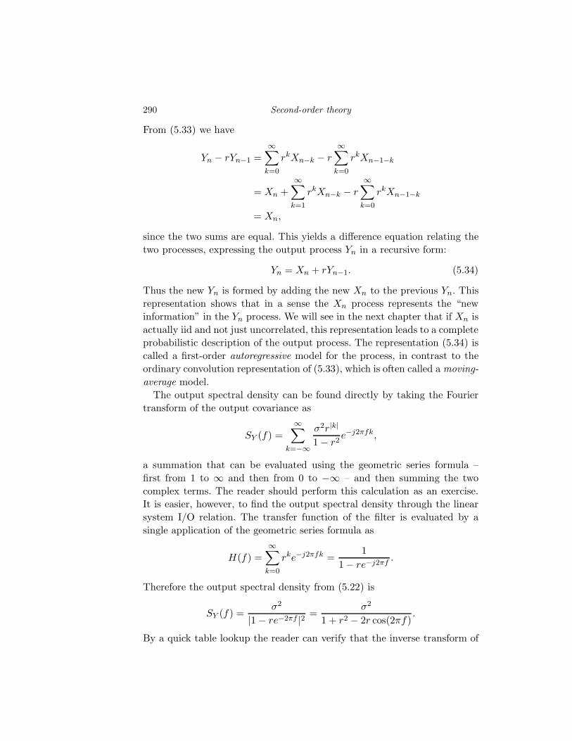
290 Second-order theory

From (5.33) we have

Yn − rYn−1 =∞∑

k=0

rkXn−k − r∞∑

k=0

rkXn−1−k

= Xn +∞∑

k=1

rkXn−k − r∞∑

k=0

rkXn−1−k

= Xn,

since the two sums are equal. This yields a difference equation relating the

two processes, expressing the output process Yn in a recursive form:

Yn = Xn + rYn−1. (5.34)

Thus the new Yn is formed by adding the new Xn to the previous Yn. This

representation shows that in a sense the Xn process represents the “new

information” in the Yn process. We will see in the next chapter that if Xn is

actually iid and not just uncorrelated, this representation leads to a complete

probabilistic description of the output process. The representation (5.34) is

called a first-order autoregressive model for the process, in contrast to the

ordinary convolution representation of (5.33), which is often called a moving-

average model.

The output spectral density can be found directly by taking the Fourier

transform of the output covariance as

SY (f) =

∞∑

k=−∞

σ2r|k|

1 − r2e−j2πfk,

a summation that can be evaluated using the geometric series formula –

first from 1 to ∞ and then from 0 to −∞ – and then summing the two

complex terms. The reader should perform this calculation as an exercise.

It is easier, however, to find the output spectral density through the linear

system I/O relation. The transfer function of the filter is evaluated by a

single application of the geometric series formula as

H(f) =

∞∑

k=0

rke−j2πfk =1

1 − re−j2πf.

Therefore the output spectral density from (5.22) is

SY (f) =σ2

|1 − re−2πf |2 =σ2

1 + r2 − 2r cos(2πf).

By a quick table lookup the reader can verify that the inverse transform of

5.4 Linearly filtered uncorrelated processes 291

the output spectral density agrees with the covariance function previously

found.

[5.2] Suppose that a one-sided uncorrelated process Xn with mean m

and variance σ2 is put into a one-sided filter with δ-response as in Ex-

ample [5.1]. Let Yn be the resulting one-sided output process. Find the

output mean and covariance.

This time (5.6) yields

EYn = mn∑

k=0

rk = m1 − rn+1

1 − r

from the geometric series formula. From (5.32) the covariance is

KY (k, j) = σ2

min(k,j)∑

n=0

r2n+|k−j| = σ2r|k−j|1 − r2(min(k,j)+1)

1 − r2.

Observe that since |r| < 1, if we let n → ∞, then the mean of this exam-

ple goes to the mean of the preceding example in the limit. Similarly, if

one fixes the lag |k − j| and lets k (and hence j) go to ∞, then in the limit

the one-sided covariance looks like the two-sided example. This simple

example points out a typical form of nonstationarity: a linearly filtered

uncorrelated process is not stationary by any definition, but as one gets

farther and farther from the origin, the parameters look more and more

stationary. This can be considered as a form of asymptotic stationarity.

In fact, a process is defined as being asymptotically weakly stationary if

the mean and covariance converge in the sense just given. One can view

such processes as having transients that die out with time. It is not

difficult to show that if a process is asymptotically weakly stationary

and if the limiting mean and covariance meet the conditions of the

ergodic theorem, then the process itself will satisfy the ergodic theorem.

Intuitively stated, transients do not affect the long-term sample averages.

[5.3] Next consider the one-sided process of Example [5.2], but now choose

the δ-response with r = 1; that is, hk = 1 for all k ≥ 0. Find the output

mean and covariance. (Note that this filter is not stable.) Applying (5.4)–

(5.6) and (5.28), (5.30), and (5.31) yields

EYn = mn∑

k=0

hk = m(n + 1)

292 Second-order theory

and

KY (k, j) = σ2(min(k, j) + 1) = σ2 min(k + 1, j + 1).

Observe that like Example [5.2], the process of Example [5.3] is not weakly

stationary. Unlike [5.2], however, it does not behave asymptotically like a

weakly stationary process – even for large time, the moments very much

depend on the time origin. Thus the nonstationarities of this process are

not only transients – they last forever! In a sense, this process is much more

nonstationary than the previous one and, in fact, does not have a mean

ergodic theorem. If the input process is Gaussian with zero mean, then we

shall see in Chapter 6 that the output process Yn is also Gaussian. Such

a Gaussian process with zero mean and with the covariance function of this

example is called the discrete time Wiener process.

[5.4] A binary Markov process

The linear filtering ideas can be applied when other forms of arithmetic

than real arithmetic is used. Rather than try to be general we illustrate

the approach by an example, a process formed by linear filtering using

binary (modulo 2) arithmetic on an iid sequence of coin flips.

Given a known input process and a filter (a modulo 2 linear recursion

in the present case), find the covariance function of the output. General

formulas will be derived later in the book; here a direct approach to the

problem at hand is taken.

First observe that KY (k, j) = E[(Yk − E(Yk))(Yj − E(Yj))] is easily eval-

uated for the case k = j because the marginal for Yk is equiprobable:

E[Yk] =∑

y

ypY (y) =1

2(0 + 1) =

1

2

KY (k, k) = σ2Y = E

[(Yk −

1

2

)2]

=∑

y

(y − 1

2

)2

pY (y) =1

2

(1

4+

1

4

)=

1

4.

As we have seen, a covariance function is symmetric in the sense that

KY (k, j) = E[(Yk − E(Yk))(Yj − E(Yj))]

= E[(Yj − E(Yj))(Yk − E(Yk))]

= KY (j, k)

so that we will be done if we evaluate KY (k, j) for the special case where

5.4 Linearly filtered uncorrelated processes 293

k = j + l for l ≥ 1. Let p be the probability of a 1 and consider therefore

KY (j + l, j) = E

[(Yj+l −

1

2

)(Yj −

1

2

)]

= E

[(Xj+l ⊕ Yj+l−1 −

1

2

)(Yj −

1

2

)]

=∑

x,y,z

(x ⊕ y − 1

2

)(z − 1

2

)pXj+l,Yj+l−1,Yj(x, y, z)

=∑

x,y,z

(x ⊕ y − 1

2

)(z − 1

2

)pXj+l

(x)pYj+l−1,Yj(y, z)

=∑

y,z

((0 ⊕ y − 1

2

)(z − 1

2

)(1 − p)pYj+l−1,Yj(y, z)

+

(1 ⊕ y − 1

2

)(z − 1

2

)p pYj+l−1,Yj(y, z)

)

.

Since 0 ⊕ y = y and 1 ⊕ y = 1 − y, this becomes

KY (j + l, j) = (1 − p)∑

y,z

(y − 1

2

)(z − 1

2

)pYj+l−1,Yj (y, z)

+p∑

y,z

(1 − y − 1

2

)(z − 1

2

)pYj+l−1,Yj (y, z)

= (1 − 2p)KY (j + l − 1, j); l = 1, 2, . . .

This is a simple linear difference equation with initial condition KY (j, j)

and hence the solution is

KY (j + l, j) = (1 − 2p)lKY (j, j) =1

4(1 − 2p)l; l = 1, 2, . . . (5.35)

(Just plug it into the difference equation to verify that it is indeed a

solution.) Invoking the symmetry property the covariance function is

given by

KY (k, j) =1

4(1 − 2p)|k−j| = KY (k − j). (5.36)

Note that KY (k) is absolutely summable (use the geometric progression)

so that the weak law of large numbers holds for the process.

294 Second-order theory

5.5 Linear modulation

In this section we consider a different form of linear system: a linear mod-

ulator. Unlike the filters considered thus far, these systems are generally

time-varying and contain random parameters. They are simpler than the

general linear filters, however, in that the output depends on the input in

an instantaneous fashion; that is, the output at time t depends only on the

input at time t and not on previous inputs.

In general, the word modulation means the methodical altering of one

waveform by another. The waveform being altered is often called a carrier,

and the waveform or sequence doing the altering, which we will model as a

random process, is called the signal. Physically, such modulation is usually

done to transform an information-bearing signal into a process suitable for

communication over a particular medium; e.g., simple amplitude modula-

tion of a carrier sinusoid by a signal in order to take advantage of the fact

that the resulting high-frequency signals will better propagate through the

atmosphere than will audio frequencies.

The emphasis will be on continuous time random processes since most

communication systems involve at some point such a continuous time link.

Several of the techniques, however, work virtually without change in a dis-

crete environment.

The prime example of linear modulation is the ubiquitous amplitude mod-

ulation or AM used for much of commercial broadcasting. If X(t) is a

continuous time weakly stationary random process with zero mean and co-

variance function KX(τ), then the output process

Y (t) = (a0 + a1X(t)) cos(2πft + θ) (5.37)

is called amplitude modulation of the cosine by the original process. The pa-

rameters a0 and a1 are called modulation constants. Amplitude modulation

is depicted in a block diagram in Figure 5.2 Observe that linear modula-

tion is not a linear operation in the normal linear systems sense unless the

constant a0 is 0. (It is, however, an affine operation – linear in the sense

that straight lines in the two-dimensional x − y space are said to be linear.)

Nonetheless, as is commonly done, we will refer to this operation as linear

modulation.

The phase term θ may be a fixed constant or a random variable, say Θ.

(We point out a subtle source of confusion here: if Θ is a random variable,

then the system is affine or linear for the input process only when the actual

sample value, say θ, of Θ is known.) We usually assume for convenience

that Θ is a random variable, independent of the X process and uniformly

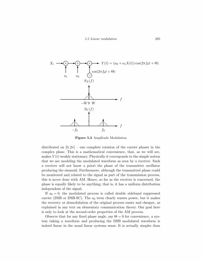
5.5 Linear modulation 295

Xt- m×

6

a1

- m+6

a2

- m×6

m∼cos(2πf0t + Θ)

- Y (t) = (a0 + a1X(t)) cos(2πf0t + Θ)

- f

6

6

SX(f)

−W 0 W

@@

- f

6SY (f)

f0

66

−f0

@@ @@

Figure 5.2 Amplitude Modulation

distributed on [0, 2π] – one complete rotation of the carrier phaser in the

complex plane. This is a mathematical convenience, that, as we will see,

makes Y (t) weakly stationary. Physically it corresponds to the simple notion

that we are modeling the modulated waveform as seen by a receiver. Such

a receiver will not know a priori the phase of the transmitter oscillator

producing the sinusoid. Furthermore, although the transmitted phase could

be monitored and related to the signal as part of the transmission process,

this is never done with AM. Hence, so far as the receiver is concerned, the

phase is equally likely to be anything; that is, it has a uniform distribution

independent of the signal.

If a0 = 0, the modulated process is called double sideband suppressed

carrier (DSB or DSB-SC). The a0 term clearly wastes power, but it makes

the recovery or demodulation of the original process easier and cheaper, as

explained in any text on elementary communication theory. Our goal here

is only to look at the second-order properties of the AM process.

Observe that for any fixed phase angle, say Θ = 0 for convenience, a sys-

tem taking a waveform and producing the DSB modulated waveform is

indeed linear in the usual linear systems sense. It is actually simpler than

296 Second-order theory

the output of a general linear filter since the output at a given time depends

only on the input at that time.

Since Θ and the X process are independent, the mean of the output is

EY (t) = (a0 + a1EX(t))E cos(2πft + Θ).

But Θ is uniformly distributed. Thus for any fixed time and frequency,

E cos(2πft + Θ) =

∫ 2π

0cos(2πft + θ)

dθ

2π

=1

2π

∫ 2π

0cos(2πft + θ) dθ = 0 (5.38)

since the integral of a sinusoid over a period is zero; hence EY (t) = 0 whether

or not the original signal has zero mean.

The covariance function of the output is given by the following expansion

of the product Y (t)Y (s) using (5.37):

KY (t, s) = a20E[cos(2πft + Θ) cos(2πfs + Θ)]

+a0a1(EX(t)E[cos(2πft + Θ) cos(2πfs + Θ)]

+ a0a1EX(s)E[cos(2πft + Θ) cos(2πfs + Θ)])

+a21KX(t, s)E[(cos 2πft + Θ)(cos 2πfs + Θ)].

Using the fact that the original process has zero mean eliminates the middle

lines in the preceding. Combining the remaining two terms and using the

cosine identity

cos x cos y =1

2cos(x + y) +

1

2cos(x − y) (5.39)

yields

KY (t, s) = (a20 + a2

1KX(t, s))

×(

1

2E cos(2πf(t + s) + 2Θ) +

1

2E cos(2πf(t − s))

).

Exactly as in the mean computation of (5.38), the expectation of the term

with the Θ in it is zero, leaving

KY (τ) =1

2(a2

0 + a21KX(τ)) cos(2πfτ).

Thus we have demonstrated that amplitude modulation of a carrier by a

weakly stationary random process results in an output that is weakly sta-

tionary.

5.6 White noise 297

The power spectral density of the AM process that we considered in the

section on linear modulation can be found directly by transforming the co-

variance function or by using standard Fourier techniques: the transform of

a covariance function times a cosine is the convolution of the original power

spectral density with the generalized Fourier transform of the cosine – that

is, a pair of impulses. This yields a pair of replicas of the original power

spectral densities, centered at plus and minus the carrier frequency f0 and

symmetric about f0, as depicted in Figure 5.2.

If further filtering is desired, e.g., to remove one of the symmetric halves

of the power spectral density to form single sideband modulation, then the

usual linear techniques can be applied, as indicated by (5.22).

5.6 White noise

Let Xn be an uncorrelated, weakly stationary, discrete time random pro-

cess with zero mean. We have seen that for such a process the covariance

function is a pulse at the origin; that is,

KX(τ) = σ2Xδτ ,

where δτ is a Kronecker delta function. As noted earlier, taking the Fourier

transform results in the spectral density

SX(f) = σ2X ; all f,

that is, the power spectral density of such a process is flat over the entire

frequency range. We remarked that a process with such a flat spectrum is

said to be white. We now make this definition formally for both discrete and

continuous time processes:

A random process Xt is said to be white if its power spectral density

is a constant for all f . (A white process is also almost always assumed to

have a zero mean, an assumption that we will make.)

The concept of white noise is clearly well defined and free of analytical

difficulties in the discrete time case. In the continuous time case, however,

there is a problem if white noise is defined as a process with constant power

spectral density for all frequencies. Recall from (5.24) that the average power

in a process is the integral of the power spectral density. In the discrete time

case, integrating a constant over a finite range causes no problem. In the

continuous time case, we find from (5.24) that a white noise process has

infinite average power. In other words, if such a process existed, it would

blow up the universe! A quick perusal of the stochastic systems literature

298 Second-order theory

shows, however, that this problem has not prevented models of continuous

time white noise processes from being popular and useful. The resolution

of the apparent paradox is fairly simple: indeed, white noise is a physically

impossible process. But there do exist noise sources that have a flat power

spectral density over a range of frequencies that is much larger than the

bandwidths of subsequent filters of measurement devices. In fact, this is

exactly the case with the thermal noise process caused by heat in resistors

in amplifier circuits. A derivation based on the physics of such a process (see

Chapter 6) yields a covariance function of the form KX(τ) = kTRαe−α|τ |,where k is Boltzman’s constant, T is the absolute temperature, and R and

α are parameters of the physical medium. The application of (5.20) results

in the power spectral density

SX(f) = kTR2α2

α2 + (2πf)2.

As α → ∞, the power spectral density tends toward the value 2kTR for all

f ; that is, the process looks like white noise over a large bandwidth. Thus,

for example, the total noise power in a bandwidth (−B,B) is approximately

2kTR × 2B, a fact that has been verified closely by experiment.

If such a process is put into a filter having a transfer function whose

magnitude become negligible long before the power spectral density of the

input process decreases much, then the output process power spectral den-

sity SY (f) = |H(f)|2SX(f) will be approximately the same at the output as

it would have been if SX(f) were flat forever since SX(f) is flat for all values

of f where |H(f)| is nonnegligible. Thus, so far as the output process is con-

cerned the input process can be either the physically impossible white noise

model or a more realistic model with finite power. However, since the input

white noise model is much simpler to work with analytically, it is usually

adopted.

In summary, continuous time white noise is often a useful model for the

input to a filter when we are trying to study the output. Commonly the input

random process is represented as being white with flat spectral density equal

to N0/2. The factor of 2 is included because of the “two-sided” nature of filter

transfer functions; a low pass filter with cutoff frequency B applied to the

white noise input will have output power equal to N0B in accordance with

(5.25). Such a white noise process makes mathematical sense only if seen

through a filter. The process itself is not rigorously defined. Its covariance

function, however, can be represented in terms of a Dirac delta function for

the purposes of analytical manipulations. Note that in (5.23) the generalized

Fourier transform of the flat spectrum results in a Dirac delta function of unit

5.6 White noise 299

impulse. In particular, if the continuous time, white noise random process

has power spectral density

SX(f) =N0

2,

then it will have a covariance or autocorrelation function

KX(τ) =N0

2δ(τ).

Thus adjacent samples of the random process are uncorrelated (and hence

also independent if the process is Gaussian) no matter how close together

in time the samples are. At the same time, the variance of a single sample

is infinite. Clearly such behavior is physically impossible. It is reasonable,

however, to state qualitatively that adjacent samples are uncorrelated at all

times greater than the shortest time delays in subsequent filtering.

Perhaps the nicest attribute of white noise processes is the simple form

of the output power spectral density of a linear filter driven by white noise.

If a discrete or continuous time random process has power spectral density

SX(f) = N0/2 for all f and it is put into a linear filter with transfer function

H(f), then from (5.22) the output process Yt has power spectral density

SY (f) = |H(f)|2 N0

2. (5.40)

The result given in (5.40) is of more importance than first appearances

indicate. A basic result of the theory of weakly stationary random processes,

called the spectral factorization theorem, states that if a random process

Yt has a spectral density SY (f) such that∫

ln SY (f) df > −∞ (discrete time) (5.41)

or∫

ln SY (f)

1 + f2df > −∞ (continuous time), (5.42)

then the power spectral density has the form of (5.40) for some causal lin-

ear stable time-invariant filter. That is, the second-order properties of any

random process satisfying these conditions can be modeled as the output

of a causal linear filter driven by white noise. Such random processes are

said to be physically realizable and comprise most random processes seen in

practice. The conditions (5.41)–(5.42) are referred to as the Paley–Wiener

criteria[70]. This result is of extreme importance in estimation, detection,

prediction, and system identification. We note in passing that in such mod-

300 Second-order theory

els the white noise driving process is called the innovations process of the

output process if the filter has a causal and stable inverse.

As a word of caution, there do exist processes which are not “physically

realizable” in the above sense of violating the Paley–Wiener criteria (5.41

- 5.42), yet which are still “physically realizable” in the sense that simple

models describe the processes. Consider the following example suggested to

the authors by A. V. Balakrishnan: let X be a zero-mean Gaussian random

variable with variance 1 and let Θ be a random variable with a uniform dis-

tribution on [−π, π) which is independent of X. Define the random process

Y (t) = cos(Xt − Θ). Then analogous to the development of the autocorre-

lation function for linear modulation, we have that

E[Y (t)] = E[cos(Xt − Θ)] = 0

RY (τ) = E[cos(Xt − Θ) cos(X(t − τ) − Θ)]

=1

2E[cos(Xτ)] =

1

4E[ejτX + e−jτX ]

=1

4(MX(jτ) + MX(−jτ)) =

1

2e−τ2

so that the power spectral density is

SY (f) =1

2e−f2

, (5.43)

which fails to meet the Paley–Wiener criterion for a continuous time random

process.

5.6.1 Low pass and narrow band noise

Suppose that white noise is put through a filter with transfer function H(f)

which has magnitude 1 for f ∈ [−W,W ] and is zero elsewhere. This will

produce a process with a flat power spectral density in a low frequency

range, a process sometimes referred to as low band noise or baseband noise.

If the original input is Gaussian, than the output low band noise process

will also be Gaussian. Now suppose that this process, say nc(t), is put into

an AM system. Then by an obvious modification of Figure 5.2 the resulting

process will be flat within a band around ±f0 and 0 elsewhere, an example

of narrow band noise.

5.7 ⋆Time averages 301

5.7 ⋆Time averages

Recall the definitions of mean, autocorrelation, and covariance as expecta-

tions of samples of a weakly stationary random process Xn; n ∈ Z:

m = E[Xn]

RX(k) = E[XnX∗n−k]

KX(k) = E[(Xn − m)(Xn−k − m)∗] = RX(k) − |m|2.

These are collectively considered as the second-order moments of the process.

The corresponding time-average moments can be described if the limits are

assumed to exist in some suitable sense:

M = < Xn >= limN→∞

1

N

N−1∑

n=0

Xn

RX(k) = < XnX∗n−k >= lim

N→∞1

N

N−1∑

k=0

XnX∗n−k

KX(k) = < (Xn − m)(Xn−k − m)∗ >

= limN→∞

1

N

N−1∑

n=0

(Xn − m)(Xn−k − m)∗.

Keep in mind that these quantities, if they exist at all, are random variables.

For example, if we actually view a sample function Xn(ω); n ∈ Z, then

the sample autocorrelation is

RX(k) = limN→∞

1

N

N−1∑

k=0

Xn(ω)X∗n−k(ω),

also a function of the sample point ω and hence a random variable. Of

particular interest is the autocorrelation for 0 lag:

PX = RX(0) = limN→∞

1

N

N−1∑

k=0

|Xn|2,

which can be considered as the sample- or time-average power of the sam-

ple function in the sense that it is the average power dissipated in a unit

resistance if Xn corresponds to a voltage.

Analogous to the expectations, the time-average autocorrelation function

and the time-average covariance function are related by

KX(k) = RX(k) − |M|2. (5.44)

302 Second-order theory

In fact, subject to suitable technical conditions as described in the laws of

large numbers, the time averages should be the same as the expectations,

that is, under suitable conditions a weakly stationary random process Xnshould have the properties that

m = MRX(k) = RX(k)

KX(k) = KX(k),

which provides a suggestion of how the expectations can be estimated in

practice. Typically the actual moments are not known a priori, but the

random process is observed over a finite time N and the results used to

estimate the moments, e.g., the sample mean

MN =1

N

N−1∑

n=0

Xn

and the sample autocorrelation function

RN (k) =1

N

N−1∑

n=0

XnX∗n−k.

These provide intuitive estimates of the actual moments which should con-

verge to the true moments as N → ∞.

There are in fact many ways to estimate second-order moments and there

is a wide literature on the subject. For example, the observed samples may

be weighted or “windowed” so as to diminish the impact of samples in the

distant past or near the borders of separate blocks of data which are han-

dled separately. The literature on estimating correlations and covariances is

particularly rich in the speech processing area.

If the process meets the conditions of the law of large numbers, then its

sample-average power PX will be RX(0), which is typically some nonzero

positive number. But if the limit limN→∞ (1/N)∑N−1

n=0 |Xn|2 is not zero,

then observe that necessarily the limit

limN→∞

N−1∑

n=0

|Xn|2 =

∞∑

n=0

|Xn|2

must blow up since it lacks the normalizing N in the denominator. In other

words, a sample function with nonzero average power will have infinite en-

ergy. The point of this observation is that a sample function from a perfectly

reasonable random process will not meet the conditions for the existence of a

5.7 ⋆Time averages 303

Fourier transform, which suggests we might not be able to apply the consid-

erable theory of Fourier analysis when considering the behavior of random

processes in linear systems. Happily this is not the case, but Fourier analysis

of random processes will be somewhat different from the Fourier analysis of

deterministic finite energy signals and of deterministic periodic signals.

To motivate a possible remedy, first “window” the sample signal Xn; n ∈Z to form a new signal X(N)

n ; n ∈ Z defined by

X(N)n =

Xn if n ≤ N − 1

0 otherwise. (5.45)

The new random process X(N)n clearly has finite energy (and is absolutely

summable) so it has a Fourier transform in the usual sense, which can be

defined as

XN (f) =

∞∑

n=0

X(N)n e−j2πfn =

N−1∑

n=0

Xne−j2πfn,

which is the Fourier transform or spectrum of the truncated sample signal.

Keep in mind that this is a random variable. It depends on the underlying

sample point ω through the sample waveform selected. From Parceval’s (or

Plancherel’s) theorem, the energy in the truncated signal can be evaluated

from the spectrum as

EN =

N−1∑

n=0

|Xn|2 =

∫ 1/2

−1/2|XN (f)|2 df. (5.46)

The average power is obtained by normalizing the average energy by the

time duration N :

PN =1

N

N−1∑

n=0

|Xn|2 =1

N

∫ 1/2

−1/2|XN (f)|2 df. (5.47)

Because of this formula |XN (f)|2/N can be considered as the power spectral

density of the truncated waveform because, analogous to a probability den-

sity or a mass density, it is a nonnegative function which when integrated

gives the power. Unfortunately it gives only the power spectral density for

a particular truncated sample function. What is really desired is a notion

of power spectral density for the entire random process. An alternative def-

inition of power spectral density resolves these two issues by taking the

expectation to get rid of the randomness, and using the limit to look at the

entire signal, that is, to define the average power spectral density as the

304 Second-order theory

limit (if it exists)

limN→∞

E(|XN (f)|2)N

.

To evaluate this limit consider

limN→∞

E(|XN (f)|2)N

= limN→∞

1

NE

(

|N−1∑

k=0

Xke−i2πfk|2

)

= limN→∞

1

NE

(N−1∑

k=0

N−1∑

l=0

Xke−i2πfkX∗

l e+i2πfl

)

= limN→∞

1

N

N−1∑

k=0

N−1∑

l=0

E[XkX∗l ]e−i2πf(k−l)

= limN→∞

1

N

N−1∑

k=0

N−1∑

l=0

RX(k − l)e−i2πf(k−l)

= limN→∞

N−1∑

k=−(N−1)

(1 − |k|N

)RX(k)e−i2πfk,

where the last term involves reordering terms using Lemma B.1 (analogous

to what was done to prove the law of large numbers for asymptotically

uncorrelated weakly stationary processes). If the autocorrelation function is

absolutely summable, i.e., if

∞∑

k=−∞|RX(k)| < ∞, (5.48)

then Lemma B.2 implies that

limN→∞

E(|XN (f)|2)N

=

∞∑

k=−∞RX(k)e−i2πfk = SX(f), (5.49)

the power spectral density as earlier defined.

5.8 ⋆Mean square calculus

The goal of this section is to develop in some detail the ideas that permit a

rigorous approach to several of the results developed earlier in this chapter.

We consider only one approach to rigor, that of mean square calculus. There

are others, but the mean square calculus approach is popular for engineering

applications because the details involve techniques already considered – in

5.8 ⋆Mean square calculus 305

particular the idea of mean square convergence. Although the correctness

of the informally derived results is usually simply assumed by engineering

practitioners, it can prove useful when developing new models to be aware

of the kinds of conditions necessary for the good behavior and correctness

of many common tools, including limits, interchanging limits and expecta-

tions, integration, and differentiation. In other words, we look deeper into

one approach to calculus for random processes. As with ordinary calculus,

arguably the key underlying idea is that of a limit, and in this section the

limit used is the limit in mean square. This section is strongly influenced

by unpublished notes of Wilbur B. Davenport, Jr., from MIT course 6.573

in fall 1965, and on the first author’s notes taken in that course. Material

has been added to put mean square convergence into the context of metric

spaces, linear normed spaces, Hilbert spaces, Banach spaces, and L2 spaces

to provide an explicit connection to the mathematical literature, especially

functional analysis.

5.8.1 Mean square convergence revisited

Recall that a sequence of real random variables Yn is said to converge in

mean square to a random variable Y if E[Y 2n ] < ∞ all n and

limn→∞

E(|Yn − Y |2) = 0

in which case we write

Y = l.i.m.n→∞

Yn.

Mean square convergence of random variables can be viewed as simply an

engineering interpretation of the mathematical topics in analysis and func-

tional analysis of L2 convergence. A brief consideration of the mathematical

point of view can provide some useful geometric interpretations of both the

convergence and of some of its properties and implications. The reader is

referred to the literature, e.g., [1] or [32] section 2.5, for extensive treatments

of such spaces.

Since random variables are functions on probability spaces, convergence

of random variables is just an example of convergence of functions. Suppose

we have a probability space (Ω,F , P ) and we define L2 to be the space of

all complex-valued random variables with finite second moment, that is, if

X ∈ L2, then

E[|X|2] < ∞,

306 Second-order theory

where the expectation is with respect to the probability measure P . We

consider two random variables (functions) to be the same if they are equal

with probability one. The L2 space is also referred to as the space of square-

integrable functions.

We can treat this space of random variables or functions like ordinary

Euclidean space in many ways. In Euclidean space we can define a metric

|x| which denotes the “size” of a member of the space (the Euclidean distance

to the origin) and a distance between any two members of the space x and

y by the Euclidean distance

d(x, y) = |x − y|.

The notions of a metric and distance lead to many useful ideas in geometry

and calculus. For example, to say that a sequence xn converges to x can be

defined by

limn→∞

d(xn, x) = limn→∞

|xn − x| = 0.

These notions in the real line or in k-dimensional Euclidean vector space

can be extended to any space of objects for which we can define a distance

or norm.

In general, a space A is called a metric space if for every pair of points

a, b ∈ A there is an associated nonnegative real number d(a, b) called a dis-

tance or metric such that

d(a, b) = 0 if and only if a = b, (5.50)

d(a, b) = d(b, a) (symmetry), (5.51)

d(a, b) ≤ d(a, c) + d(c, b), all c ∈ A (triangle inequality). (5.52)

If A is the real line, then the magnitude of the difference between two points

trivially meets these conditions and is therefore a metric.

An example of a general metric space that is also inspired by Euclidean

space is a normed linear space. A normed linear vector space is a space A

with norm |.| and distance d(a, b) = |a − b|. A vector space or linear space

A is a space consisting of points called vectors and two operations – one

called addition which associates with each pair of vectors a, b a new vector

a + b ∈ A and one called multiplication which associates with each vector

a and each number r ∈ ℜ (called a scalar) a vector ra ∈ A – for which the

usual rules of arithmetic hold, that is, if a, b, c ∈ A and r, s ∈ ℜ, then

5.8 ⋆Mean square calculus 307

a + b = b + a (commutative law)

(a + b) + c = a + (b + c) (associative law)

r(a + b) = ra + rb (left distributive law)

(r + s)a = ra + sa (right distributive law)

(rs)a = r(sa) (associative law for multiplication)

1a = a.

In addition, it is assumed that there is a zero vector, also denoted 0, for

which

a + 0 = a

0a = 0.

We also define the vector −a = (−1)a. A normed linear space is a linear

vector space A together with a function ||a|| called a norm defined for each

a such that for all a, b ∈ A and r ∈ ℜ, ||a|| is nonnegative and

‖a‖ = 0 if and only if a = 0, (5.53)

‖a + b‖ ≤ ‖a‖ + ‖b‖ (triangle inequality). (5.54)

‖ra‖ = |r|‖a‖. (5.55)

Returning to the space L2 it is easy to see that it is a linear space since lin-

ear combinations of random variables with finite second moment have finite

second moments (just use the Cauchy–Schwarz inequality)(Problem 4.20),

that

‖X − Y ‖ =√

E[|X − Y |2] (5.56)

satisfies the conditions for a norm (remembering that two random variables

are considered equal in this space if they are equal with probability one),

and that

d(X,Y ) = ‖X − Y ‖ (5.57)

satisfies the requirements for a distance.

It can now be recognized that mean square convergence of Yn to Y is

almost identical to L2 convergence of Yn to Y in the sense that d(Yn, Y ) → 0

or ‖Yn − Y ‖ → 0. The only difference is that in the definition of mean square

308 Second-order theory

convergence we have not required that the limit random variable Y is itself

in L2, that is, it might not have a finite second or even first moment. These

observations bring into play the entire theory of normed spaces and metric

spaces when interpreting or applying mean square convergence.

As yet a third mathematical formulation note that we can define an inner

product in L2 by

(X,Y )∆= E[XY ∗] (5.58)

and use the inner product to define a norm and a distance

‖X‖ = (X,X) (5.59)

d(X,Y ) = ‖X − Y ‖. (5.60)

In general, an inner product space (or pre-Hilbert space) A is a linear space

such that for each pair a, b ∈ A there is a real number (a, b) called an inner

product such that for a, b, c ∈ A, r ∈ ℜ

(a, b) = (b, a)

(a + b, c) = (a, c) + (b, c)

(ra, b) = r(a, b)

(a, a) ≥ 0 and (a, a) = 0 if and only if a = 0.

An inner product (·, ·) then determines a distance d(a, b) = ||a − b||, where

||a|| = (a, a)1/2 is a norm.

By mimicking well-known properties of the real line, we have seen that

there is a similar structure on the space L2 of all random variables with

a finite second moment and that mean square convergence is simply an

example of convergence in a metric space, a normed linear space, and a pre-

Hilbert space. We consider one more technical property of the real line which

is less familiar, but often useful in proofs involving mean square convergence.

Suppose A is a metric space (e.g., the real line, L2, or any other normed

linear space or pre-Hilbert space). If a sequence xn ∈ A has the property

that the double limit

lim limn.m→∞

d(xn, xm) = 0,

then the sequence is called a Cauchy sequence. In other words, a sequence

xn is Cauchy if for every ǫ > 0 there is an integer N such that d(xn, xm) <

ǫ if n ≥ N and m ≥ N . A metric space is complete if every Cauchy sequence

converges; that is, if xn is a Cauchy sequence, then there is an x in A for

which x = limn→∞ xn. In the words of Simmons [62], p. 71, a complete metric

5.8 ⋆Mean square calculus 309

space is one wherein “every sequence that tries to converge is successful.” A

standard result of elementary real analysis is that Euclidean space (with the

Euclidean distance) is complete (see Rudin [61], p. 46). A complete inner

product space is called a Hilbert space. A complete normed space is called a

Banach space.

At this point the reader may be somewhat overwhelmed by the profuse

family connections of the space of random variables with finite second mo-

ments, but the primary point is to demonstrate that with all these con-

nections the theory of mean square convergence can draw upon a wealth of

literature and results and that this explains the common occurrence of these

names in the signal processing literature. Those who pursue advanced topics

in signal processing will almost certainly run into various branches of these

topics. Here we collect some of the standard properties for future use.

Lemma 5.1 Let L2 be the space of all random variables with finite second

moments. All random variables Xn and Yn for all n are assumed to be in

L2.

1. Completeness L2 is complete, that is, if Xn is a Cauchy sequence, then there is

a random variable X ∈ L2 such that l.i.m.n→∞ Xn = X.

2. Linearity Limits in the mean combine in a linear fashion (like ordinary limits),

that is, if l.i.m.n→∞ Xn = X and l.i.m.n→∞ Yn = Y , then for any constants a, b

l.i.m.n→∞

(aXn + bYn) = aX + bY. (5.61)

3. If X ∈ L2, then

E(|X |) ≤ ‖X‖. (5.62)

4. Convergence of expectation Suppose that Y = l.i.m.n→∞ Yn, then

limn→∞

E(Yn) = E(l.i.m.n→∞

Yn). (5.63)

The result shows that the common engineering practice of interchanging limits

and expectation works for random variables when the limit inside of the expecta-

tion is a limit in mean square.

5. Convergence of correlation Suppose that X and Y have finite second moments

and that l.i.m.n→∞ Xn = X and l.i.m.n→∞ Yn = Y , then

limn,m→∞

E[XnY ∗m] = E[XY ∗], (5.64)

that is, one can interchange expectation and limits when computing correlations

in the sense that

limn,m→∞

E[XnY ∗m] = E[ l.i.m.

n,m→∞XnY ∗

m]. (5.65)

310 Second-order theory

Proof

1. This is a fundamental result of functional analysis and will not be proved

here. Note that it is easy to see that if l.i.m.n→∞ Xn = X , then X must be

a Cauchy sequence. This follows from the triangle inequality: given ǫ pick N

so large that ‖X − Xn‖ ≤ ǫ/2 and ‖X − Xm‖ ≤ ǫ/2 and then observe that

‖Xn − Xm‖ ≤ ‖Xn − X‖ + ‖Xm − X‖ ≤ ǫ so that the sequence is Cauchy.

2. The linearity follows easily using the triangle inequality and is left as an exercise.

3. Equation (5.62) follows from the Cauchy–Schwarz inequality since

E(|X |) = E(|X × 1|) ≤ ‖X‖ × ‖1‖ = ‖X‖.

4. 0 ≤ |E(Yn) − E(Y )|2 = |E(Y − Yn)|2 ≤ E(|Y − Yn|2) where the last inequality

uses the Cauchy–Schwarz inequality (see Problem 4.20) Since the rightmost term

goes to zero with n by assumption, the claim is proved.

5. Use the Cauchy–Schwarz inequality:

|E[XnY ∗m − XY ∗]| = |E[XnY ∗

m − XY ∗m + XY ∗

m − XY ∗]|= |E[(Xn − X)Y ∗

m] + E[X(Ym − Y )∗]|≤ |E[(Xn − X)Y ∗

m]| + |E[X(Ym − Y )∗]|≤ E[|(Xn − X)Y ∗

m|] + E[|X(Ym − Y )∗|]≤ ‖Xn − X‖ × ‖Ym‖ + ‖X‖ × ‖Ym − Y ‖= ‖Xn − X‖ × ‖Ym − Y + Y ‖ + ‖X‖ × ‖Ym − Y ‖≤ ‖Xn − X‖ × (‖Ym − Y ‖ + ‖Y ‖) + ‖X‖ × ‖Ym − Y ‖

which tends to 0 as n and m go to infinity. 2

Throughout this section we will be approximating a random process at time

t, say X(t), by a sequence of processes, say XN (t) as N → ∞. The final

lemma of this subsection builds on the previous lemma to demonstrate the

crucial role played by second-order moments – autocorrelations in particular

– in studying mean square convergence.

Lemma 5.2 Given a sequence of random processes XN (t); t ∈ T for

which

E[|XN (t)|2] < ∞ for all t ∈ T , N = 1, 2, . . . ,

then

X(t) = l.i.m.N→∞

XN (t) (5.66)

where

E[|X(t)|2] < ∞ (5.67)

5.8 ⋆Mean square calculus 311

iff

limN,M→∞

E[XN (t)X∗M (t)] = RX(t, t), (5.68)

in which case also

limN→∞

RXN(t, s, ) = RX(t, s). (5.69)

Proof The final part of the preceeding lemma with XN = XN (t), X = X(t),

YM = XM (s), Y = X(s) yields (5.69) and with t = s yields the “only if”

statement. For the converse suppose (5.68) holds. Then

E[|XN (t) − XM (t)|2] =E[XN (t)X∗N (t)] − E[XN (t)X∗

M (t)]

− E[XM (t)X∗N (t)] + E[XM (t)X∗

M (t)],

where all of the terms on the right go to 0 as N,M → ∞, so XN (t) is a

Cauchy sequence and must have a limit in the mean with a finite second

moment from the previous lemma. 2

5.8.2 Integrating random processes

It has been noted that some care is required to extend the notion of integrals

over time from waveforms to random processes. One way of accomplishing

this is to extend the usual definition of Riemann integrals as a limit of sums

of samples to a corresponding limit of sums of random variables, where

the limit is in the sense of mean squared convergence. In this subsection

we develop this idea further and use it to provide conditions under which

the integrals exist. Suppose that x(t) has an ordinary Riemann integral

I =∫ ba x(t) dt. This will be the case if the sums

IN =

N∑

n=1

x(tn)∆tn

where a = t0 < t1 < t2 < · · · tN−1 < tN = b, and ∆tn = (tn − tn−1)/(b − a)

(we have suppressed the dependence of the sample times tn on N) will have

a unique limit as N → ∞ regardless of how the sample times are chosen

provided that the differences satisfy

limN→∞

maxn:0≤n≤N

∆tn = 0.

For example, a bounded function x(t) on a bounded interval [a, b] will have

a Riemann integral if and only if it is continuous almost everywhere in the

312 Second-order theory

interval. In this case the integral is given by the limit of sums

I = limN→∞

IN .

Now suppose that X(t) is a continuous time random process with a

finite second moment E[|X(t)|2] < ∞ for all t and we again choose sample

times with vanishing differences as above. Define the sum

IN =

N∑

n=1

X(tn)∆tn,

where now the sum is itself a random variable. Since each X(tn) has finite

second moment, the triangle inequality implies that IN also has finite second

moment since

‖IN‖ =

∥∥∥∥∥

N∑

n=1

X(tn)∆tn

∥∥∥∥∥ ≤N∑

n=1

‖X(tn)‖∆tn.

If there exists a random variable I such that

I = l.i.m.N→∞

IN = l.i.m.N→∞

N∑

n=1

X(tn)∆tn,

then I is the mean square integral of the given random process over [a, b]

and we write

I =

∫ b

aX(t) dt

∆= l.i.m.

N→∞

N∑

n=1

X(tn)∆tn.

Note that even though we use the familar Riemann notation for an integral,

this is not a Riemann integral. In particular, it is a random variable!

To explore further, suppose that the mean square integral I exists. Lemma

5.1 implies that if I itself has a finite second moment, then the integral

will behave in the expected sense that one can interchange expectation and

integration so that the expected value of the integral satisfies

E[I] = E[l.i.m.N→∞

IN ] = limN→∞

E[IN ]

= limN→∞

E[

N∑

n=1

X(tn)∆tn] = limN→∞

N∑

n=1

E[X(tn)]∆tn,

where in the final step we have used the linearity of expectation. The right-

most expression, however, is the Riemann integral of the mean function

E[X(t)]. This Riemann integral must be finite since it is equal to E[I],

5.8 ⋆Mean square calculus 313

which is finite from Lemma 5.1 since I is assumed to be in L2. Thus the

existence of the mean squared integral with a finite second moment ensures

that the mean function of the original random process has a finite Riemann

integral.

Next consider the second-order moment. Again assume that the mean

square integral I exists and has a finite second moment,

E[|I|2] = E[

∣∣∣∣∫ b

aX(t) dt

∣∣∣∣2

].

Analogous to the corresponding result for Riemann integration, it is easy to

show that for the mean square integral

∣∣∣∣∫ b

aX(t) dt

∣∣∣∣2

=

(∫ b

aX(t) dt

)×(∫ b

aX∗(s) ds

)

=

∫ b

a

∫ b

aX(t)X∗(s) dt ds (5.70)

so that interchanging expectation and integration using Lemma 5.1

E[|I|2] = E

[∫ b

a

∫ b

aX(t)X∗(s) dt ds

]

=

∫ b

a

∫ b

aE[X(t)X(s)] dt ds

=

∫ b

a

∫ b

aRX(t, s) dt ds.

Since I has a finite second moment, the double Riemann integral of the

correlation function exists and is finite. We have now proved half of the

following result, which shows that the converse is true as well and thus gives

a necessary and sufficient condition for the existence of the mean square

integral of a continuous time random process with a finite second moment.

Lemma 5.3 A continuous time random process X(t) has a mean square

integral over [a, b] with a finite second absolute moment if and only if

∫ b

a

∫ b

aRX(t, s) dt ds < ∞. (5.71)

that is, the integral exists and is finite.

Proof We have already proved the “only if” part. Suppose for the converse

314 Second-order theory

that (5.71) holds and consider

E[IN − IM |2] = E[(IN − IM )(I∗N − I∗M )]

= E[IN I∗N ] − E[IN I∗M ] − E[IM I∗N ] + E[IM I∗M ]. (5.72)

Consider for example the term

E[IN I∗M ] = E

(

N∑

i=1

X(ti)∆ti

)

M∑

j=1

X∗(tj)∆tj

=

N∑

i=1

M∑

j=1

X(ti)X∗(tj)∆ti∆tj =

N∑

i=1

M∑

j=1

R(ti, tj)∆ti∆tj.

By assumption the double Riemann integral of the autocorrelation exists

and is finite, so

limN,M→∞

E[IN I∗M ] =

∫ b

a

∫ b

aRX(t, s) dt ds < ∞.

Every one of the four terms in (5.72) converges in the same way to the same

thing and hence the sum is 0 since two are positive and two are negative.

Thus

limN,M→∞

‖IN − IM‖ = 0

and IN is a Cauchy sequence, which from Lemma 5.1 must converge to a

random variable I with a finite second moment. 2

Observe that if either condition of the lemma is met, then we have shown

that we can exchange the expectation with the mean square integral:

∫ b

aE[X(t)] dt = E

[∫ b

aX(t) dt

](5.73)

∫ b

a

∫ b

aRX(t, s) dt ds = E

[∫ b

a

∫ b

aX(t)X(s) dt ds

]. (5.74)

5.8.3 Linear filtering

As an application of mean square integration, we can now define a linear

filter operating on a continuous time random process X(t); t ∈ T , where

for convenience we consider T = (−∞,∞). Define the output process Y (t)

of a linear filter described by a weighting function h(t, τ) as a mean square

5.8 ⋆Mean square calculus 315

integral (if it exists)

Y (t) =

∫ b

aX(τ)h(t, τ) dτ, (5.75)

i.e.,

Y (t) = l.i.m.N→∞

YN (t)

where

YN (t)∆=

N∑

n=1

X(τn)h(t, τi)∆τn.

From Lemma 5.3 this integral will be well defined and have a finite second

moment if and only if

∫ b

a

∫ b

ah(t, τ)h(t, τ ′)RX(τ, τ ′) dτ dτ ′ < ∞

in which case∫ b

aE[Y (t)] dt = E

[∫ b

aX(τ)h(t, τ) dτ

](5.76)

and∫ b

a

∫ b

ah(t, τ)RX (τ, τ ′)h∗(s, τ ′) dτ dτ ′

=

∫ b

a

∫ b

aE[h(t, τ)X(τ)X∗(τ ′)h∗(s, τ ′)] dτ dτ ′

= E

[∫ b

a

∫ b

aX(τ)h(t, τ)X∗(τ ′)h∗(s, τ ′) dτdτ ′

]

= E[Y (t)Y ∗(s)] < ∞. (5.77)

This provides an alternative derivation of the output autocorrelation func-

tion and shows that its finiteness ensures the existence and finite second

absolute moment of the limit in the mean defining the output process pro-

vided the output autocorrelation is finite.

Note that if the original process is Gaussian, then the sums YN (t) are

Gaussian. Since YN (t) converges to Y (t) in mean square, it also converges

in distribution so that Y (t) is also Gaussian for each N . This is not enough

to prove that the mean square integral Y (t) is a Gaussian process, but the

idea can be extended to vectors of samples to provide a careful proof that

316 Second-order theory

the process put out by a linear filter with a Gaussian process input is also

Gaussian.

Extra work is needed to extend these ideas to integrals over infinite limits.

5.8.4 Differentiating random processes

We have said that linear systems can often be described by means other

than convolution integrals, e.g., difference equations for discrete time and

differential equations in continuous time. Here we explore the I/O relations

for a simple continuous time differentiator in order to demonstrate some of

the techniques involved for handling such systems. In addition, the results

developed will provide another interpretation of white noise.

Suppose now that we have a continuous time random process X(t); t >

0 and we form a new random process Y (t) by differentiating; that is,

Y (t) =d

dtX(t).

Here we assume X(t) to be a zero-mean random process for simplicity. Re-

sults for nonzero-mean processes are found by noting that X(t) can be writ-

ten as the sum of a zero-mean random process plus the mean function m(t).

That is, we can write X(t) = X0(t) + m(t) where X0(t) = X(t) − m(t).

Then, the derivative of X(t) is the derivative of a zero-mean random process

plus the derivative of the mean function. The derivative of the mean function

is a derivative in the usual sense and hence provides no special problems.

As with integration, there is a problem in interpreting what the derivative

means when the thing being differentiated is a random process. A derivative

is defined as a limit, and as we found in Chapter 4, there are several notions

of limits of sequences of random variables. Care is required because the

limit may exist in one sense but not necessarily in another. In particular,

two natural definitions for the derivative of a random process correspond to

convergence with probability one and convergence in mean square. As a first

possibility we could assume that each sample function of Y (t) is obtained by

differentiating each sample function of X(t); that is, we could use ordinary

differentiation on the sample functions. This gives us a definition of the form

Y (t, ω) =d

dtX(t, ω) = lim

∆t→0

X(t + ∆t, ω) − X(t, ω)

∆t.

If P (ω : the limit exists) = 1, then the definition of differentiation corre-

sponds to convergence with probability one. Alternatively, we could define

Y (t) as a limit in quadratic mean of the random variables (X(t + ∆t) −

5.8 ⋆Mean square calculus 317

X(t))/∆t as ∆t goes to zero (which does not require that the derivative

exist with probability one on sample functions). With this definition we

obtain

Y (t) = l.i.m.∆t→0

X(t + ∆t) − X(t)

∆t.

Clearly a choice of definition of derivative must be made in order to develop

a theory for this simple problem and, more generally, for linear systems

described by differential equations. Consistent with the approach of this

section, we focus on mean square convergence. First, however, we sketch a

heuristic development with the assumption that all of the derivatives exist

as required. We will blithely ignore careful specification of conditions under

which the formulas make sense during the initial pass. (Mathematicians

sometimes refer to such derivations as formal developments: techniques are

used as if they are applicable to see what happens. This often provides the

answer to a problem, which, once known, can then be proved rigorously to

be correct.) After the nonrigorous development we shall return to provide

some rigor to the key points using mean square calculus.

Define a process Y∆t(t) for a fixed ∆t as the following difference, which

approximates the derivative of X(t):

Y∆t(t) =X(t + ∆t) − X(t)

∆t.

This difference process is perfectly well defined for any fixed ∆t > 0 and in

some sense it should converge to the desired Y (t) as ∆t → 0. We can easily

find the following correlation:

E[Y∆t(t)Y∆s(s)]

= E

[X(t + ∆t) − X(t)

∆t

X(s + ∆s) − X(s)

∆s

]

=RX(t + ∆t, s + ∆s) − RX(t + ∆t, s) − RX(t, s + ∆s) + RX(t, s)

∆t∆s.

If we (formally) let ∆t and ∆s go to zero, then, if the various limits exist,

this formula becomes

RY (t, s) =∂

∂t∂sRX(t, s). (5.78)

As previously remarked, we will not try to specify complete conditions

under which this sleight of hand can be made rigorous. Suffice it to say that

if the conditions on the X process are sufficiently strong, the formula is valid.

Intuitively, since differentiation and expectation are linear operations, the

318 Second-order theory

formula follows from the assumption that the linear operations commute, as

they usually do. There are, however, serious issues of existence involved in

making the proof precise.

One obvious regularity condition to apply is that the double derivative

of (5.78) exists. If it does and the processes are weakly stationary, then

we can transform (5.78) by using the property of Fourier transforms that

differentiation in the time domain corresponds to multiplication by −j2πf

in the frequency domain. Then for the double derivative to exist we obtain

the requirement that for the spectral density of Y (t) to have finite second

moments, i.e., if SY (f) = (2πf)2SX(f), then

∫ ∞

−∞SY (f) df < ∞. (5.79)

As a rather paradoxical application of (5.78), suppose that we have a

one-sided continuous time Gaussian random process X(t); t ≥ 0 that has

zero mean and a covariance function that is the continuous time analog of

Example [5.3]; that is, KX(t, s) = σ2 min(t, s). (The Kolmogorov construc-

tion guarantees that there is such a random process; that is, that it is well

defined.) This process is known as the continuous time Wiener process, a

process that we will encounter again in the next chapter. Strictly speaking,

the double derivative of this function does not exist because of the discon-

tinuity of the function at t = s. From engineering intuition, however, the

derivative of such a step discontinuity is an impulse, suggesting that

RY (t, s) = σ2δ(t − s),

the covariance function for Gaussian white noise! Because of this formal re-

lation, Gaussian white noise is sometimes described as the formal derivative

of a Wiener process. We have to play loose with mathematics to find this

result, and the sloppiness cannot be removed in a straightforward manner.

In fact, it is known from the theory of Wiener processes that they have the

strange attribute of producing with probability one sample waveforms that

are continuous but nowhere differentiable. Thus we are considering white

noise as the derivative of a process that is not differentiable. Nonetheless,

this is a useful intuition that is consistent with the extremely pathological

behavior of sample waveforms of white noise – an idealized concept of a

process that cannot really exist.

Now return to the issue of rigor in defining the derivative of a random

process. As with mean square integration, the idea is to look at Cauchy

sequences. The proof is very similar. The following lemma summarizes the

5.8 ⋆Mean square calculus 319

results. We continue to consider zero-mean real-valued random processes for

simplicity.

Lemma 5.4 Given a zero-mean real-valued random process X(t) with fi-

nite second moments E[|X(t)|2] < ∞, then the mean square derivative

Y (t) = l.i.m.∆→0

X(t + ∆) − X(t)

∆(5.80)

will exist and have a finite second moment at t if and only if the correlation

function

∂2RX(τ, τ ′)∂τ∂τ ′

is well defined at τ = τ ′ = t, in which case

RY (t, s) =∂2RX(t, s)

∂t∂s. (5.81)

When the mean square derivative exists, it is often denoted X ′(t).

Proof Because of the similarity of the proof to that of the mean square

integration result, we only present a brief sketch. Define as before Y∆(t) =

(X(t + ∆) − X(t)/∆ and consider

‖Y∆ − Y∆′‖2

= E

[∣∣∣∣X(t + ∆) − X(t)

∆− X(t + ∆′) − X(t)

∆′

∣∣∣∣2]

= E

[∣∣∣∣X(t + ∆) − X(t)

∆

∣∣∣∣2]− 2E

[∣∣∣∣X(t + ∆) − X(t)

∆

∣∣∣∣

∣∣∣∣X(t + ∆′) − X(t)

∆′

∣∣∣∣

]

+E

[∣∣∣∣X(t + ∆′) − X(t)

∆′

∣∣∣∣2]

.

The leftmost term in the final formula is

E

[∣∣∣∣X(t + ∆) − X(t)

∆

∣∣∣∣2]

= E

[X(t + ∆)2 − 2X(t + ∆)X(t) + X(t)2

∆2

]

=RX(t + ∆, t + ∆) − 2RX(t + ∆, t) + RX(t, t)

∆2.

This second-order difference will converge to the second-order partial deriva-

tive of RX(τ, τ ′) evaluated at τ = τ ′ = t if and only if the said derivative is

well defined. Thus Y∆(t) will be a Cauchy sequence in L2 if and only if the

said derivative is well defined, in which case Y∆(t) converges in mean square.

320 Second-order theory

The remainder of the lemma follows by interchanging the expectation and

limits. 2

5.8.5 Fourier series

As another application of mean square convergence we consider Fourier series

for periodic random processes. From basic Fourier analysis recall that if

x(t); t ∈ (−∞,∞) is a periodic function with period T , i.e., if x(t + T ) =

x(t), then subject to suitable techincal conditions we can expand x(t) in a

Fourier series

x(t) =

∞∑

n=−∞X (n)e+j2πnt/T , where X (n)

∆=

1

T

∫ T

0x(t)e−j2πnt/T dt (5.82)

is the Fourier transform of one period of the function x(t). Note also that a

Fourier series can be used to represent a function x(t); t ∈ [0, T ) defined

only on the interval [0, T ).

Consider the extension of this idea to a random process. Suppose that

X(t); t ∈ (−∞,∞) is a weakly stationary zero-mean process with auto-

correlation function RX(τ). We further assume that the process is periodic

with period T in the sense that

RX(τ + T ) = RX(τ); all τ. (5.83)

If a random process is periodic in this sense, then for any t expanding the

magnitude square gives

E[|X(t) − X(t + τ)|2] = 2RX(0) − RX(τ) − RX(−τ) = 0

which from the Markov inequality implies that Pr(|X(t) − X(t + τ)| > 0) =

0, so that with probability one X(t + T ) = X(t).

Define the Fourier coefficients of the random process by the mean square

integrals

X (n) =1

T

∫ T

0X(t)e−(j2πnt/T )(j2πnt/T ) dt. (5.84)

From Lemma 5.3 this will exist iff∫ T

0

∫ T

0RX(t, s)e−j2πnt/T e+j2πns/T dt ds

=

∫ T

0

∫ T

0RX(t − s)e−j2πn(t−s)/T dt ds < ∞.

In order to ensure the existence, we assume that RX satisfies this equation.

5.8 ⋆Mean square calculus 321

Note, however, two things. First, since both RX and e−j2πnt/T are periodic

with period T , taking the integral over T results in the same value regardless

of s so that the constraint becomes∫ T

0RX(t)e−j2πnt/T dt < ∞. (5.85)

Second, note that since RX(t) is periodic with period T , assuming it is well

behaved it has a Fourier series

RX(τ) =∞∑

n=−∞bne+j2πnt/T (5.86)

where

bn =1

T

∫ T

0RX(τ)e−j2πnt/T dt (5.87)

so that our constraint for existence of the mean square integral is simply

that the Fourier coefficients of RX be finite. Assuming this to be the case,

then the correlation of the Fourier coefficients of X(t) can be evaluated as

E[X (n)X ∗(m)]

= E

[(1

T

∫ T

0X(t)e−j2πnt/T dt

)(1

T

∫ T

0X(s)e−j2πms/T ds

)]

=1

T 2

∫ T

0

∫ T

0RX(t − s)e−j2π(nt−ms)/T dt ds

=1

T 2

∫ T

0e−j2π(n−m)s/T

∫ T

0RX(t − s)e−j2πn(t−s)/T dt ds

= bn

∫ 1

0e−j2π(n−m)s ds = bnδn−m,

so that the Fourier coefficients are orthogonal random variables.

We now have all the needed machinery to prove the following lemma

characterizing the existence of Fourier series of random processes.

Lemma 5.5 Suppose that X(t); t ∈ ℜ is a weakly stationary random pro-

cess for which the RX(τ) is periodic and has a Fourier series. Then the mean

square integrals

X (n) =1

T

∫ T

0X(t)e−j2πnt/T dt (5.88)

exist and have finite second moment,

E[X (n)X ∗(m)] = E[|Xn|2δn−m], (5.89)

322 Second-order theory

and

X(t) = l.i.m.n→∞

N∑

n=−N

X (n)e+j2πnt/T . (5.90)

Conversely, if X(t); t ∈ ℜ is a random process for which (5.88) exists for

all n and (5.89)–(5.90) hold, then X(t) is weakly stationary and periodic.

Proof We have already shown that if X(t) is weakly stationary, periodic,

and its autocorrelation RX(τ) has a Fourier series, then (5.88)–(5.89) hold.

To prove (5.90) define XN (t) =∑N

n=−N X (n)e+j2πnt/T and we have

E[|X(t) − XN (t)|∗]= E[X(t)X∗(t)] − E[X(t)X∗

N (t)] − E[XN (t)X∗(t)] + E[XN (t)X∗N (t)]

= RX(0) − E

[

X(t)

N∑

n=−N

X ∗(n)e−j2πnt/T

]

− E

[

X∗(t)N∑

n=−N

X (n)e+j2πnt/T

]

+E

[N∑

n=−N

X (n)e+j2πnt/TN∑

n=−N

X ∗(n)e−j2πnt/T

]

= RX(0) −N∑

n=−N

E

[X(t)

1

T

∫ T

0X∗(s)e+j2πns/T ds

]e−j2πnt/T

−N∑

n=−N

E

[X∗(t)

1

T

∫ T

0X(s)e−j2πns/T ds

]e+j2πnt/T

+

N∑

n=−N

N∑

m=−N

E[X (n)X ∗(m)]

= RX(0) −N∑

n=−N

1

T

∫ T

0RX(t − s)e−j2πn(t−s)/T ds

−N∑

n=−N

1

T

∫ T

0RX(s − t)e−j2πn(s−t)/T ds +

N∑

n=−N

bn

= RX(0) −N∑

n=−N

bn.

From Parceval’s theorem for Fourier series,

RX(0) =∞∑

n=−∞bn

5.8 ⋆Mean square calculus 323

and hence

limN→∞

E[|X(t) − XN (t)|∗] = limN→∞

( ∞∑

n=−∞bn −

N∑

n=−N

bn

)= 0,

proving (5.90).

For the converse, assume (5.88)–(5.90) hold. From Lemma 5.2 we now

that

RX(t, s) = limN→∞

RXN(t, s) (5.91)

and we evaluate

RXN(t, s) = E[XN (t)X∗

N (s)]

= E[

N∑

n=−N

X (n)e+j2πnt/TN∑

m=−N

X ∗(m)e−j2πms/T ]

=N∑

n=−N

N∑

m=−N

E[X (n)X ∗(m)]e+j2π(nt−ms)/T

=N∑

n=−N

E[|X (n)|2]e+j2πn(t−s)/T ,

which is weakly stationary and periodic with period T for all N , hence the

limit also be weakly stationary and periodic with period T . 2

Thus a zero-mean continuous time random process can be expanded in a

mean square Fourier series with uncorrelated coefficients if and only if it is

weakly stationary and periodic.

5.8.6 Sampling

A key step in converting an analog signal processing problem into a digi-

tal signal processing problem is sampling a continuous time process X(t)

to produce a discrete time process Xn = X(nT ) = X(n/f0) using a sam-

pling interval of T seconds or a sampling frequency of W = 1/T samples per

second. It is a standard result of Fourier analysis and basic linear systems

theory that if the Fourier transform of a deterministic signal x(t) is zero out-

side some frequency range [−W0,W0], then provided the sampling frequency

W is fast enough, W > W0, or the sampling interval or period T = 1/2W is

short enough, T ≤ 1/2W0, then the original signal can in theory be recovered

324 Second-order theory

from its samples using the sampling expansion

x(t) =

∞∑

n=−∞x(nT )

sin(π(t − nT )/T )

π(t − nT )/T. (5.92)

The sampling expansion is sometimes interpreted as pulse amplitude modula-

tion since a sequence of “pulses” of the form sin(π(t − nT )/T )/π(t − nT )/T

are multiplied or modulated by the samples x(nT ) and the resulting wave-

form allows the reconstruction of the original time function. In this sub-

section we use the ideas of mean square convergence to derive a sampling

theorem for continuous time random processes. Here we state the result and

devote the remainder of the subsection to deriving it.

Before proceeding to the case of random processes, it will be useful to

provide a simple proof of the deterministic case using Fourier series. By

assumption x(t) has a Fourier transform

X (f) =

∫ ∞

∞x(t)e−j2πft dt

and the original signal x(t) can be recovered by inverting the Fourier trans-

form,

x(t) =

∫ ∞

−∞X (f)e+j2πft df (5.93)

which is 0 for f 6∈ (−W,W ). Thus we can expand X on the interval [−W,W ]

in a Fourier series as

X (f) =

∞∑

n=−∞ane−j2πnf/2W

an =1

2W

∫ W

−WX (f)e+j2πnf/2W df

=1

2W

∫ ∞

−∞X (f)e+j2πnf/2W df =

1

2Wx( n

2W

)

using (5.93). Thus the transform of x(t) can be expressed in terms of the

samples of x(nT ) by

X (f) =∞∑

n=−∞Tx(nT )e−j2πnf/2W . (5.94)

5.8 ⋆Mean square calculus 325

Inverting the transform then yields the sampling expansion:

x(t) =

∫ W

−WX (f)e+j2πft df

=

∫ W

−W

∞∑

n=−∞

1

2Wx( n

2W

)e−j2πnf/2W e+j2πft df

=∞∑

n=−∞

1

2Wx( n

2W

)∫ W

−We+j2πf(t−n/2W ) df

=

∞∑

n=−∞

1

2Wx( n

2W

) sin(π(t − nT )/T )

π(t − nT )/T

as claimed.

As a special case that will be useful later, observe that x(t) =

sin(π(t − s)/T ))/π(t − s)/T ) has a transform that meets the constraint –

its Fourier transform is a box function at the origin running from −W to

W . Thus applying the ordinary sampling theorem to this function yields the

identity

sin(π(t − s)/T ))

π(t − s)/T )=

∞∑

n=−∞

sin(π(nT − s)/T )

π(nT − s)/T

sin(π(t − nT )/T )

π(t − nT )/T. (5.95)

Theorem 5.1 The mean square sampling theorem

Given a continuous time weakly stationary random process with zero mean

and a power spectral density SX(f) with the property that

SX(f) = 0 for |f | ≥ W, (5.96)

then for any T ≤ 1/2W

X(t) = l.i.m.N→∞

N∑

n=−N

X(nT )sin(π(t − nT )/T )

π(t − nT )/T. (5.97)

Proof Define

XN (t) =

N∑

n=−N

X(nT )sin(π(t − nT )/T )

π(t − nT )/T

326 Second-order theory

and consider

E[|X(t) − XN (t)|2]

= E[|X(t) −N∑

n=−N

X(nT )sin(π(t − nT )/T )

π(t − nT )/T|2]

= E[X(t)X∗(t)] −N∑

n=−N

E[X(t)X∗(nT )]sin(π(t − nT )/T )

π(t − nT )/T

−N∑

n=−N

E[X∗(t)X(nT )]sin(π(t − nT )/T )

π(t − nT )/T

+

N∑

n=−N

N∑

m=−N

E[X(nT )X∗(mT )]sin(π(t − nT )/T )

π(t − nT )/T

sin(π(t − mT )/T )

π(t − mT )/T

so that

E[|X(t) − XN (t)|2]

= RX(0) −N∑

n=−N

RX(t − nT )sin(π(t − nT )/T )

π(t − nT )/T(5.98)

−N∑

n=−N

RX(nT − t)sin(π(t − nT )/T )

π(t − nT )/T(5.99)

+

N∑

n=−N

N∑

m=−N

RX((n − m)T )

× sin(π(t − nT )/T )

π(t − nT )/T

sin(π(t − mT )/T )

π(t − mT )/T. (5.100)

The second and third terms above resemble a sampling expansion of the au-

tocorrelation RX , which is reasonable since its Fourier transform is assumed

to be band-limited. To be more precise, consider the function RX(t − τ) as

a function of t. From Fourier transform theory its transform is SX(f)ej2πfτ ,

which is band-limited. Hence we have the sampling expansion

RX(t − τ) =∞∑

n=−∞RX (nT − τ)

sin(π(t − nT )/T )

π(t − nT )/T. (5.101)

5.8 ⋆Mean square calculus 327

Setting τ = t results in

RX(0) =

∞∑

n=−∞RX (nT − t)

sin(π(t − nT )/T )

π(t − nT )/T.

This shows that the third term (5.99) converges to RX(0) and the same

argument holds for the second term (5.100). This leaves the fourth term

(5.100). Rewrite the term as

N∑

n=−N

N∑

m=−N

RX((n − m)T )sin(π(t − nT )/T )

π(t − nT )/T

sin(π(t − mT )/T )

π(t − mT )/T

=2N∑

k=−2N

RX(kT )

×∑∑

n,m:n−m=k,−N≤m,n≤N

sin(π(t − nT )/T )

π(t − nT )/T

sin(π(t − mT )/T )

π(t − mT )/T.

As N → ∞ the kth term in the summand converges to

∑∑n,m:n−m=k

sin(π(t − nT )/T )

π(t − nT )/T

sin(π(t − mT )/T )

π(t − mT )/T

=

∞∑

n=−∞

sin(π(t − nT )/T )

π(t − nT )/T

sin(π(t + kT − nT )/T )

π(t + kT − nT )/T=

sin(πk)

πk,

where (5.95) was used in the last step. Thus

limN→∞

N∑

n=−N

N∑

m=−N

RX((n − m)T )sin(π(t − nT )/T )

π(t − nT )/T

sin(π(t − mT )/T )

π(t − mT )/T

=

∞∑

−∞RX(k)

sin(πk)

πk= RX(0)

and the proof is complete. 2

5.8.7 Karhunen–Loeve expansion

Let X(t); t ∈ ℜ be a zero-mean random process with finite second moment

and autocorrelation function RX(t, s). Consider a generalization of a Fourier

series where a random process is represented as a linear combination of func-

tions with certain specified properties. Specifically we seek a representation

of the form

X(t) = l.i.m.n→∞

XN (t) (5.102)

328 Second-order theory

for t ∈ [a, b], where

XN (t)∆=

N∑

n=1

Xnφn(t) (5.103)

Xn =

∫ b

aX(t)φ∗

n(t) dt (5.104)

∫ b

aφn(t)φ∗

m(t) dt = δn−m (5.105)

E[XmX∗n] = λnδn−m (5.106)

We refer to such an expansion (if it exists) as a Karhunen–Loeve expansion

of the random process.

If (5.102) holds, then from Lemma 5.2

RX(t, s) = limN→∞

RXN(t, s)

where we use the assumed properties to compute

RXN(t, s) = E[XN (t)X∗

N (s)] = E

[N∑

n=1

Xnφn(t)

N∑

m=1

X∗mφ∗

m(t)

]

=N∑

n=1

N∑

m=1

E[XnX∗m]φn(t)φ∗

m(t)] =N∑

n=1

λNφn(t)φ∗n(t)

so that

RX(t, s) = limN→∞

RXN(t, s) =

∞∑

n=1

λnφn(t)φ∗n(t).

Multiplying by a φ-function and integrating then yields

∫ b

aRX(t, s)φm(s) ds =

∞∑

n=1

λnφn(t)

∫ b

aφm(s)φ∗

n(s) ds

= λnφn(t).

Thus if we wish to have a representation satisfying (5.102)–(5.105), then the

φ-functions and energies λ must satisfy∫ b

aRX(t, s)φ(s) ds = λφ(t), (5.107)

that is, the φs must be eigenfunctions of the above integral equation with

eigenvalue λ. In fact, this is an “if and only if” statement, that is, φn are

the eigenfunctions and λn the eigenvalues satisfying (5.107) if and only if

5.8 ⋆Mean square calculus 329

(5.102)–(5.105) hold. To prove this, we next show that if φn and λn satisfy

(5.107), then indeed (5.102)–(5.105) hold. We normalize eigenfunctions to

have unit energy,∫ b

a|φ(t)|2 dt = 1

and absorb the normalization in the eigenvalue λ. First suppose that φn and

φm are distinct eigenfunctions of (5.107) with eigenvalues λn and λm. We

show that this implies that φn and φm are orthogonal in that (5.105) holds

and that λn is real and nonnegative, so it indeed is a valid energy for a

random variable. By assumption

λnφn(t) =

∫ b

aRX(t, s)φn(s) ds

so that multiplying both sides by φm(t) for any m (including n) and inte-

grating we have

λn

∫ b

aφ∗

m(t)φn(t) dt =

∫ b

a

∫ b

aφ∗

m(t)RX(t, s)φn(s) ds dt

=

∫ b

aφn(s)

(∫ b

aRX(t, s)φ∗

m(t)

)ds

=

∫ b

aφn(s)

(∫ b

aRX(s, t)φm(t)

)∗ds

= λ∗m

∫ b

aφn(t)φ∗

m(t) dt

so that

(λn − λ∗m)

∫ b

aφn(t)φ∗

m(t) dt = 0.

If n = m this implies that

(λn − λ∗n)

∫ b

a|φn(t)|2 dt = (λn − λ∗

n) = 0,

which forces λn to be real. For n 6= m we have

(λn − λm)

∫ b

aφn(t)φ∗

m(t) dt = 0.

If λn 6= λm, then φn and φm must be orthogonal. If the two eigenvalues are

equal, then we have to work harder and quote material beyond the mathe-

matical scope of this book to prove the desired result. It turns out (see, e.g.,

330 Second-order theory

Appendix 2 of [14]) that there are at most a countably infinite number of dis-

tinct eigenfunctions. Each eigenfunction can have associated with it at most

a finite number of linearly independent eigenfunctions and these eigenfunc-

tions can be transformed by linear operations into a set of an equal number

of orthogonal unit energy eigenfunctions using a Gram–Schmidt procedure.

Thus any distinct eigenvalues automatically yield orthogonal eigenfunctions,

while equal eigenvalues can correspond to several eigenfunctions which can

be made orthogonal by linear operations.

Given now the collection φn of orthogonal and normalized eigenfunctions,

we have

E[XnX∗m] = E

[(∫ b

aX(t)φ∗

n(t) dt

)(∫ b

aX(s)φm(s) ds

)]

=

∫ b

a

∫ b

aE[X(t)X∗(s)]φ∗

n(t)φm(s) ds dt

=

∫ b

a

(∫ b

aRX(t, s)φm(s) ds

)φ∗

n(t) dt

=

∫ b

aλmφm(t)φ∗

n(t) dt = λnδn−m,

so that the Xn are indeed uncorrelated. To prove mean square convergence

consider as usual

E[|X(t) − XN (t)|2] =

E[X(t)X(t)∗] − E[X(t)XN (t)∗] − E[XN (t)X(t)∗] + E[XN (t)XN (t)∗].

The first term is RX(t, s). The second term is

E[X(t)XN (t)∗] = E

[X(t)

N∑

n=1

X∗nφ∗

n(t)

]=

N∑

n=1

E[X(t)X∗n]φ∗

n(t)]

=

N∑

n=1

E

[X(t)

∫ b

aX∗(s)φn(s) ds]φ∗

n(t)

]

=

N∑

n=1

φ∗n(t)

∫ b

aE[X(t)X∗(s)]φn(s) ds

=N∑

n=1

φ∗n(t)

∫ b

aRX(t, s)φn(s) ds =

N∑

n=1

φ∗n(t)φ∗

n(t).

5.8 ⋆Mean square calculus 331

A similar evaluation shows that

E[XN (t)X(t)∗] =

N∑

n=1

φ∗n(t)φ∗

n(t),

and

E[XN (t)XN (t)∗] = E

[N∑

n=1

Xnφn(t)

N∑

m=1

X∗mφ∗

m(t)

]

=N∑

n=1

N∑

m=1

E[XnX∗m]φn(t)φ∗

m(t)

=

N∑

n=1

λnφn(t)φ∗n(t)

so that

limn→∞

E[|X(t) − XN (t)|2] = RX(t, t) −∞∑

n=1

λnφn(t)φ∗n(t). (5.108)

Once again we invoke a result from the theory of integral equations: Mercer’s

theorem (see, e.g., Appendix 2 of [14]) states that under suitable conditions

– including the case where RX(t, s) is continuous in t and s over [a, b], the

right-hand side above is 0 and mean square convergence is proved.

As a first example, suppose that X(t) is weakly stationary and periodic

with period T and hence that RX(τ) is periodic. If RX has a Fourier series

expansion

RX(τ) =∞∑

n=−∞bnej2πnτ/T

then the integral equation (5.107) to be solved for the Karhunen–Loeve

expansion is

λφ(t) =

∫ T

0

∞∑

n=−∞bnej2πn(t−s)/T φ(s) ds =

∞∑

n=−∞bn

∫ T

0ej2πn(t−s)/T φ(s) ds.

Guessing a solution φn(t) = cnej2πnt/T where cn is a normalizing constant,

then∫ T

0cnej2πnt/T cm ∗ e−j2πmt/T dt = cnc∗m

∫ t

0ej2π(n−m)t/T dt

= |cn|2TδN−M

332 Second-order theory

so that cn = 1/√

T . Then with

φn(t) =ej2πnt/T

√T

the integral equation becomes

λej2πnt/T

√T

=∞∑

n=−∞bn

∫ T

0ej2πn(t−s)/T ej2πns/T

√T

ds

=

∞∑

n=−∞bn

ej2πnt/T

√T

∫ T

0e

j2π(m−n)sT ds

= bmTej2πnt/T

√T

= bmTφm(t),

which we already knew was a solution from the development for Fourier

series.

As another example, suppose that X(t) is white noise with SX(f) = N0/2

for all f and hence RX(τ) = (N0/2)δ(τ), a Dirac delta. In this case

∫ b

aRX(t − s)φ(s) ds =

N0

2

∫ b

aδ(t − s)φ(s) ds

=N0

2φ(t) = λφ(t),

yielding the strange behavior that all eigenvalues are identical so that all

terms in the Karhunen–Loeve representation have the same second moment.

5.9 ⋆Linear estimation and filtering

In this section we give another application of second-order moments in lin-

ear systems by showing how they arise in one of the basic problems of

communication; estimating the outcomes of one random process based on

observations of another process using a linear filter. The initial results can

be viewed as process variations on the vector results of Section 4.11, but we

develop them independently here in the process and linear filtering context

for completeness. We will obtain the classical orthogonality principle and the

Wiener–Hopf equation and consider solutions for various simple cases. This

section provides additional practice in manipulating second-order moments

of random processes and provides more evidence for their importance.

We will focus on discrete time for the usual reasons, but the continuous

time analogs are found, also as usual, by replacing the sums by integrals.

5.9 ⋆Linear estimation and filtering 333

5.9.1 Discrete time

Suppose that we are given a record of observations of values of one random

process; e.g., we are told the values of Yi; N < i < M, and we are asked

to form the best estimate of a particular sample, say Xn, of another, related

random process Xk; k ∈ T . We refer to the collection of indices of observed

samples as K = (N,M). We permit N and M to take on infinite values. For

convenience we assume throughout this section that both processes have

zero means for all time. We place the strong constraint on the estimate that

it must be linear; that is, the estimate Xn of Xn must have the form

Xn =∑

k:n−k∈KhkYn−k =

∑

k∈Khn−kYk

for some δ-response h. We wish to find the “best” possible filter h, perhaps

under additional constraints such as causality. One possible notion of best

is to define the error

ǫn = Xn − Xn

and define that filter to be best within some class if it minimizes the mean

squared error E(ǫ2n); that is, a filter satisfying some constraints will be con-

sidered optimum if no other filter yields a smaller expected squared error.

The filter accomplishing this goal is often called a linear least squared error

(LLSE) filter.

Many constraints on the filter or observation times are possible. Typical

constraints on the filter and on the observations are the following:

1. We have a noncausal filter that can “see” into the infinite future and a two-sided

infinite observation Yk; k ∈ Z. Here we consider N = −∞ and M = ∞. This

is clearly not completely possible, but it may be a reasonable approximation for

a system using a very long observation record to estimate a sample of a related

process in the middle of the records.

2. The filter is causal (hk = 0 for k < 0), a constraint that can be incorporated

by assuming that n ≥ M ; that is, that samples occurring after the one we wish

to estimate are not observed. When n > M the estimator is sometimes called a

predictor since it estimates the value of the desired process at a time later than

the last observation. Here we assume that we observe the entire past of the Y

process; that is, we take N = −∞ and observe Yk; k < M. If, for example, the

X process and the Y process are the same and M = n, then this case is called

the one-step predictor (based on the semi-infinite past).

3. The filter is causal, and we have a finite record of T seconds; that is, we observe

Yk; M − T ≤ K < M.

334 Second-order theory

As one might suspect, the fewer the constraints, the easier the solution but

the less practical the resulting filter. We will develop a general characteriza-

tion for the optimum filters, but we will provide specific solutions only for

certain special cases. We formally state the basic result as a theorem and

then prove it.

Theorem 5.2 Suppose that we are given a set of observations Yk; k ∈ Kof a zero-mean random process Yk and that we wish to find a linear esti-

mate Xn of a sample Xn of a zero-mean random process Xn of the form

Xn =∑

k:n−k∈KhkYn−k. (5.109)

If the estimation error is defined as

ǫn = Xn − Xn,

then for a fixed n no linear filter can yield a smaller expected squared error

E(ǫ2n) than a filter h (if it exists) that satisfies the relation

E(ǫnYk) = 0; all k ∈ K, (5.110)

or, equivalently,

E(XnYk) =∑

i:n−i∈KhiE(Yn−iYk); all k ∈ K. (5.111)

If RY (k, j) = E(YkYj) is the autocorrelation function of the Y process and

RX,Y (k, j) = E(XkYj) is the cross-correlation function of the two processes,

then (5.111) can be written as

RX,Y (n, k) =∑

i: n−i∈KhiRY (n − i, k); all k ∈ K. (5.112)

If the processes are jointly weakly stationary in the sense that both are in-

dividually weakly stationary with a cross-correlation function that depends

only on the difference between the arguments, then, with the replacement of

k by n − k, the condition becomes

RX,Y (k) =∑

i:n−i∈KhiRY (k − i); all k : n − k ∈ K. (5.113)

Comments. Two random variables U and V are said to be orthogonal if

E(UV ) = 0. Therefore (5.110) is known as the orthogonality principle be-

cause it states that the optimal filter causes the estimation error to be or-

thogonal to the observations. Note that (5.110) implies not only that the

5.9 ⋆Linear estimation and filtering 335

estimation error is orthogonal to the observations, but that it is also orthog-

onal to all linear combinations of the observations. Relation (5.113) with

K = (−∞, n) is known as the Wiener–Hopf equation. For this to be useful

in practice, we must be able to find a δ-response that solves one of these

equations. We shall later find solutions for some simple cases. A more gen-

eral treatment is beyond the intended scope of this book. Our emphasis here

is to demonstrate an example in which determination of an optimal filter

for a reasonably general problem requires the solution of an equation given

in terms of second-order moments.

Proof Suppose that we have a filter h that satisfies the given conditions.

Let g be any other linear filter with the same input observations and let

Xn be the resulting estimate. We will show that the given conditions imply

that g can yield an expected squared error no better than that of h. Let

ǫn = Xn − Xn be the estimation error using g so that

E(ǫ2n) = E

(

Xn −∑

i:n−i∈KgiYn−i

)2

.

Add and subtract the estimate using h satisfying the conditions of the the-

orem and expand the square to obtain

E(ǫ2n) = E

(

Xn −∑

i: n−i∈KhiYn−i +

∑

i:n−i∈KhiYn−i −

∑

i:n−i∈KgiYn−i

)2

= E

(

Xn −∑

i: n−i∈KhiYn−i

)2

+ E

(

∑

i:n−i∈K(hi − gi)Yn−i

)2

+2E

((

Xn −∑

i:n−i∈KhiYn−i

)(∑

i:n−i∈K(hi − gi)Yn−i

))

.

The first term on the right is the expected squared error using the filter

h, say E(ǫ2n). The last term on the right is the expectation of something

squared and is hence nonnegative. Thus we have the lower bound

E(ǫ2n) ≥ E(ǫ2

n) +∑

i: n−i∈K(hi − gi)

E(XnYn−i) −∑

j:n−j∈KhjE(Yn−jYn−i

,

where we have brought one of the sums out, used different dummy vari-

ables for the two sums, and interchanged some expectations and sums. From

(5.111), however, the bracketed term is zero for each i in the index set being

336 Second-order theory

summed over, and hence the entire sum is zero, proving that

E(ǫ2n) ≥ E(ǫ2

n),

which completes the proof of the theorem. 2

Note that from (5.109) through (5.113) we can write the mean square error

for the optimum linear filter as

E(ǫ2n) = E

(ǫn

(Xn −

∑

k:n−k∈KhkYn−k

))= E(ǫnXn)

= RX(n, n) −∑

k:n−k∈KhkRX,Y (n, n − k)

in general and

E(ǫ2n) = RX(0) −

∑

k:n−k∈KhkRX,Y (k)

for weakly stationary processes.

Older proofs of the result just given use the calculus of variations, that

is, calculus minimization techniques. The method we have used, however, is

simple and intuitive and shows that a filter satisfying the given equations

actually yields a global minimum to the mean squared error and not only

a local minimum as usually obtained by obtained by calculus methods. A

popular proof of the basic orthogonality principle is based on Hilbert space

methods and the projection theorem, the generalization of the standard geo-

metric result that the shortest line from a point to a plane is the projection of

the point on the plane – the line passing through the point which meets the

plane at a right angle (is orthogonal to the plane). The projection method

also proves that the filter of (5.110) yields a global minimum.

We consider four examples in which the theorem can be applied to con-

struct an estimate. The first two are fairly simple and suffice for a brief

reading.

[5.4] Suppose that the processes are jointly weakly stationary, that we are

given the entire two-sided realization of the random process Yn, and

that there are no restrictions on the linear filter h. Equation (5.113) then

becomes

RX,Y (k) =∑

i∈ZhiRY (k − i); all k ∈ Z.

5.9 ⋆Linear estimation and filtering 337

This equation is a simple convolution and can be solved by standard Fourier

techniques. Take the Fourier transform of both sides and define the trans-

form of the cross-correlation function RX,Y to be the cross-spectral density

SX,Y (f). We obtain SX,Y (f) = H(f)SY (f) or

H(f) =SX,Y (f)

SY (f),

which can be inverted to find the optimal δ-response h:

h(k) =

∫ 1/2

−1/2

SX,Y (f)

SY (f)ei2πkf df,

which yields an optimum estimate

Xn =

∞∑

i=−∞hiYn−i.

Thus we have an explicit solution for the optimal linear estimator for this

case in terms of the second-order properties of the given processes. Note,

however, that the resulting filter is not causal in general. Another important

observation is that the filter itself does not depend on the sample time n at

which we wish to estimate the X process; e.g., if we want to estimate Xn+1,

we apply the same filter to the shifted observations; that is,

Xn+1 =∞∑

i=−∞hiYn+1−i.

Thus in this example not only have we found a means of estimating Xn for

a fixed n, but the same filter also works for any n. When one filter works for

all estimate sample times by simply shifting the observations, we say that

it is a time-invariant or stationary estimator. As one might guess, such time

invariance is a consequence of the weak stationarity of the processes.

The most important application of Example [5.4] is to “infinite smooth-

ing,” where Yn = Xn + Vn. The noise process Vn is assumed to be orthogo-

nal to the signal process Xn, i.e., RX,V (k) = 0 for all k. Then RX,Y = RX

and hence RY = RX + RV , so that

H(f) =SX(f)

SX(f) + SV (f). (5.114)

[5.5] Again assume that the processes are jointly weakly stationary. As-

sume that we require a causal linear filter h but that we observe

the infinite past of the observation process. Assume further that the

observation process is white noise; that is, RY (k) = (N0/2)δk. Then

338 Second-order theory

K = n, n − 1, n − 2, . . ., and (5.113) becomes the Wiener–Hopf equa-

tion

RX,Y (k) =∑

i:n−i∈Khi

N0

2δk−i = hk

N0

2; k ∈ Z+.

This equation easily reduces because of the δ-function to

hk =2

N0RX,Y (k), k ∈ Z+.

Thus we have for this example the optimal estimator

Xn =

∞∑

k=0

2

N0RX,Y (k)Yn−k.

As with the previous example, the filter does not depend on n, and hence

the estimator is time-invariant.

The case of a white observation process is indeed special, but it suggests

a general approach to solving the Wiener–Hopf equation, which we sketch

next.

[5.6] Assume joint weak stationarity and a causal filter on a semi-infinite

observation sequence as in Example [5.5], but do not assume that the

observation process is white. In addition, assume that the observation

process is physically realizable so that a spectral factorization of the

form of (5.40) exists; that is,

SY (f) = |G(f)|2

for some causal stable filter with transfer function G(f). As previously

discussed, for practical purposes, all random processes have spectral den-

sities of this form. We also assume that the inverse filter, the filter with

transfer function 1/G(f), is causal and stable. Again, this holds under

quite general conditions. Observe in particular that you cannot run into

trouble with G(f) being zero on a frequency interval of nonzero length

because the condition in the spectral factorization theorem would be

violated.

Unlike the earlier examples, this example does not have a trivial solution. We

sketch a solution as a modification to the solution of Example [5.5]. The given

observation process may not be white, but suppose that we pass it through a

linear filter r with transfer function R(f) = 1/G(f) to obtain a new random

process, say Wn. Since the inverse filter 1/G(f) is assumed stable, then the

W process has power spectral density SW (f) = SY (f)|R(f)|2 = 1 for all f ;

5.9 ⋆Linear estimation and filtering 339

that is, Wn is white. One says that the W process is a whitened version of

the Y process, sometimes called the innovations process of Yn. Intuitively,

the W process contains the same information as the Y process from it by

passing it through the filter G(f) (at least in principle). Thus we can get an

estimate of Xn, from the W process that is just as good as (and no better

than) that obtainable from the Y process. Furthermore, if we now filter the

W process to estimate Xn, then the overall operation of the whitening filter

followed by the estimating linear filter is also a linear filter, producing the

estimate from the original observations. Since the inverse filter is causal, a

causal estimate based on the W process is also a causal estimate based on

the Y process.

Because W is white, the estimate of Xn from Wn is given immediately

by the solution to Example [5.5]; that is, the filter h with the W process

as input is given by hk = RX,W (k) for k ≥ 0. The cross-correlation of the

X and W processes can be calculated using the standard linear filter I/O

techniques. It turns out that the required cross-correlation is the inverse

Fourier transform of a cross-spectral density given by

SX,W (f) =SX,Y (f)

G(f∗)= H(f), (5.115)

where the asterisk denotes the complex conjugate. (See Problem 5.21.) Thus

the optimal causal linear estimator given the whitened process is

hk =

∫ 1/2−1/2

SX,Y (f)G(f)∗ e2πjkf k ≥ 0

0 otherwise,

and the overall optimal linear estimate has the form shown in Figure 5.3.

Yn- 1

G-Wn

hk- Xn

Whitening filter Estimator for X given W

Figure 5.3 Prewhitening method

Although more complicated, we again have a filter that does not depend

on n.

This approach to solving the Wiener–Hopf equation is called the

“prewhitening” (or “innovations” or “shaping filter”) approach and it can

340 Second-order theory

be made rigorous under quite general conditions. That is, for all practical

purposes, the optimal filter can be written in this cascade form as a whiten-

ing filter followed by a LLSE filter given the whitened observations as long

as the processes are jointly weakly stationary and we know the observation

process’s power spectral density.

When the observation interval is finite or when the processes are not

jointly weakly stationary, the spectral factorization approach becomes com-

plicated and cumbersome, and alternative methods, usually in the time do-

main, are required. The final example considers such an estimator.

[5.7] Suppose that the random process we wish to estimate satisfies a

difference equation of the form

Xn+1 = ΦnXn + Un , n ≥ 0, (5.116)

where the process Un is a zero-mean process that is uncorrelated with

a possibly time-varying second moment E(U2n) = Γn and X0 is an initial

random variable, independent of the Un. Φn is a known sequence of

constants. In other words, we know that the random process is defined

by a time-varying linear system driven by noise that is uncorrelated but

not necessarily stationary. Assume that the observation process has the

form

Yn = HnXn + Vn, (5.117)

a scaled version of the X process plus observation noise, where Hn is a

known sequence of constants. We also assume that the observation noise

has zero mean and is uncorrelated but not necessarily stationary, say

E(V 2n ) = Ψn. We further assume that the U and V processes are uncor-

related: E(UnVk) = 0 for all n and k. Intuitively, the random processes

are such that new values are obtained by scaling old values and adding

some perturbations. Additional noise influences our observations. Sup-

pose that we observe Y0, Y1, . . . , Yn−1, what is the best linear estimate of

Xn?

In a sense this problem is more restrictive than the Wiener–Hopf formula-

tion of Example [5.6] because we have assumed a particular structure for the

process to be estimated and for the observations. On the other hand, it is not

a special case of the previous model because the time-varying parameters

make it nonstationary and because we restrict the observations to a finite

time window (not including the current observation), often a better approx-

imation to reality. Because of these differences the spectral techniques of the

standard Wiener–Hopf solution of Example [5.6] do not apply without signif-

5.9 ⋆Linear estimation and filtering 341

icant generalization and modification. Hence we consider another approach,

called recursive estimation . The technique has its origins in the work of

Gauss on plotting the trajectory of heavenly bodies [25]. The method was

developed in 1958 by Swerling[65] and subsequently refined and publicized

by Kalman and Bucy. The technique is now generally known as Kalman–

Bucy filtering, . The basic idea is the following: instead of considering how to

operate on a complete observation record in order to estimate something at

one time, suppose that we already have a good estimate Xn for Xn and that

we make a single new observation Yn. How can we use this new information

to update our old estimate in a linear fashion to form a new estimate Xn+1

of Xn+1? For example, can we find sequences of numbers an and bn so that

Xn+1 = anXn + bnYn

is a good estimate? One way to view this is that instead of constructing a

filter h described by a convolution that operates on the past to produce an

estimate for each time, we wish a possibly time-varying filter with feedback

that observes its own past outputs or estimates and operates on this and

a new observation to produce a new estimate. This is the basic idea of

recursive filtering, which is applicable to more general models than that

considered here. In particular, the standard developments in the literature

consider vector generalizations of the above difference equations. We sketch

a derivation for the simpler scalar case.

We begin by trying to apply directly the orthogonality principle of (5.110)

through (5.112). If we fix a time n and try to estimate Xn by a linear filter

as

Xn =

n∑

i=1

hiYn−i, (5.118)

then the LLSE filter is described by the time-dependent δ-response, say

h(n−1), which, from (5.112), solves the equations

RX,Y (n, l) =

n∑

i=1

h(n−1)i RY (n − i, l); l = 0, 1, . . . , n − 1, (5.119)

where the superscript reflects the fact that the estimate is based on obser-

vations through time n − 1 and the fact that for this very nonstationary

problem, the filter will likely depend very much on n. To demonstrate this,

342 Second-order theory

consider the estimate for Xn+1. In this case we will have a filter of the form

Xn+1 =

n+1∑

i=1

h(n)i Yn+1−i, (5.120)

where the LLSE filter satisfies

RX,Y (n + 1, l) =n+1∑

i=1

h(n)i RY (n + 1 − i, l); l = 0, 1, . . . , n. (5.121)

Note that (5.121) is different from (5.119), and hence the δ-responses satisfy-

ing the respective equations will also differ. In principle these equations can

be solved to obtain the desired filters. Since they will in general depend on

n, however, we are faced with the alarming possibility of having to apply for

each time n a completely different filter h(n) to the entire record of observa-

tions Y0, . . . , Yn up to the current time, clearly an impractical system design.

We shall see, however, that a more efficient means of recursively computing

the estimate can be found. It will still be based on linear operations, but

now they will be time-varying.

We begin by comparing (5.119) and (5.121) more carefully to find a re-

lation between the two filters h(n) and h(n − 1). If we consider l < n, then

(5.116) implies that

RX,Y (n + 1, l) = E(Xn+1Yl) = E((ΦnXn + Un)Yl)

= ΦnE(XnYl) + E(UnYl) = ΦnE(XnYl)

= ΦnRX,Y (n, l).

Reindexing the sum of (5.121) using this relation and restricting ourselves

to l < n then yields

ΦnRX,Y (n, l) =

n∑

i=0

h(n)i+1RY (n − i, l)

= h(n)1 RY (n, l) +

n∑

i=1

h(n)i+1RY (n − i, l), l = 0, 1, . . . , n − 1.

But for l < n we also have that

RX,Y (n, l) = E(Xn, Yl) = E

(Yn − Vn

HnYl

)

=1

HnE(YnYl) =

1

HnRY (n, l)

5.9 ⋆Linear estimation and filtering 343

or

RY (n, l) = HnRX,Y (n, l).

Substituting this result, we have with some algebra that

RX,Y (n, l) =n∑

i=1

hni+1

Φn − h(n)1 Hn

RY (n − i, l); l = 0, 1, . . . , n − 1,

which is the same as (5.119) if one identifies

h(n−1)i =

hni+1

Φn − h(n)1 Hn

; l = 1, . . . , n.

From (5.120) the estimate for Xn is

Xn =

n∑

i=1

h(n−1)i Yn−i =

1

Φn − h(n)1 Hn

n+1∑

i=2

h(n)i Yn+1−i.

Comparing this with (5.120) yields

Xn+1 = h(n)1 Yn + (Φn − h

(n)1 Hn)Xn,

which has the desired form. It remains, however, to find a means of com-

puting the numbers h(n)1 . Since this really depends on only one argument n,

we now change notation for brevity and henceforth denote this term by xn;

that is,

xn = h(n)1 .

To describe the estimator completely we need to find a means of computing

xn and an initial estimate. The initial estimate does not depend on any ob-

servations. The LLSE estimate of a random variable without observations

is the mean of the random variable (see, e.g., Problem 4.26). Since by as-

sumption the processes all have zero mean, X0 = 0 is the initial estimate.

Before computing xn, we make several remarks on the estimator and its

properties. First, we can rewrite the estimator as

Xn+1 = xn(Yn − HnXn) + ΦnXn.

It is easily seen from the orthogonality principle that if Xn is a LLSE es-

timate of Xn given Y0, Y1, . . . , Yn−1, then Yn − HnXn = Yn − Yn∆= νn can

be interpreted as the “new” information in the observation Yn in the sense

that our best prediction of Yn based on previously known samples has been

344 Second-order theory

removed from Yn. We can now write

Xn+1 = κnνn + ΦnXn.

This can be interpreted as saying that the new estimate is formed from

the old estimate by using the same transformation Φn used on the actual

samples and then by adding a term depending only on the new information.

It also follows from the orthogonality principle that the sequence νn is

uncorrelated: since HnXn is the LLSE estimate for Yn based on the pre-

vious n samples Y0, . . . , Yn−1, the error νn must be orthogonal to past Yl

from the orthogonality principle. Hence νn must also be orthogonal to linear

combinations of past Yl and hence also to past νl. It is straightforward to

show that Eνn = 0 for all n and hence orthogonality of the sequence implies

that it is also uncorrelated (Problem 5.24). Because of the various proper-

ties, the sequence νn is called the innovations sequence of the observations

process. Note the analog with Example [5.6], where the observations were

first whitened to form innovations and then the estimate was formed based

on the whitened version.

Observe next that the innovations and the estimation error are simply

related by the formula

νn = Yn − HnXn = HnXn + Vn − HnXn = Hn(Xn − Xn) + Vn

or

νn = Hnǫn + Vn,

a useful formula for deriving some of the properties of the filter. For example,

we can use this formula to find a recursion for the estimate error:

ǫ0 = X0

ǫn+1 = Xn+1 − Xn+1

= ΦnXn + Un − κnνn − ΦnXn

= (Φn − κnHn)ǫn + Un − κnVn; n = 0, 1.

(5.122)

This formula implies that

E(ǫn) = 0; n = 0, 1, . . . ,

and hence the estimate is unbiased (i.e., an estimate having an error which

has zero mean is defined to be unbiased). It also provides a recursion for

finding the expected squared estimation error:

E(ǫ2n+1) = (Φn − κnHn)2E(ǫ2

n) + E(U2n) + κ2

nE(V 2n ),

5.9 ⋆Linear estimation and filtering 345

where we have made use of the assumptions of the problem statement,

namely, the uncorrelation of Un and Vn sequences with each other, with

Y0, . . . , Yn−1, X0, . . . ,Xn, and hence also with ǫn. Rearranging terms for

later use, we have

E(ǫ2n+1) = Φ2

nE(ǫ2n) − 2κnHnΦnE(ǫ2

n) − +κ2n(H2

nE(ǫ2n) + Ψn) + Γn,

(5.123)

where Γn∆= E(U2

n) and Ψn∆= E(V 2

n ).

Since we know that E(ǫ20) = E(X2

0 ), if we knew the κn we could recursively

evaluate the expected squared errors from the formula and the given problem

parameters. We now complete the system design by developing a formula

for the κn. This is most easily done by using the orthogonality relation and

(5.122):

0 = E(ǫn+1Yn) = (Φn − κnHn)E(ǫnYn) + E(UnYn) − κnE(VnYn).

Consider the terms on the right. Proceeding from left to right, the first term

involves

E(ǫnYn) = E(ǫn(HnXn + Vn)) = HnE(ǫn(ǫn + Xn)) = HnE(ǫ2n),

where we have used the fact that ǫn is orthogonal to Vn, to Y0, . . . , Yn−1 and

hence to Xn. The second term is zero by the assumptions of the problem.

The third term requires the evaluation

E(VnYn) = E(Vn(HnXn + Vn)) = E(V 2n ).

Thus we have that

0 = (Φn − κnHn)HnE(ǫ2n) − κnE(V 2

n )

or

κn =ΦnHnE(ǫ2

n)

E(V 2n ) + H2

nE(ǫ2n)

.

Thus for each n we can solve the recursion for E(ǫ2n) and for the required

κn to form the next estimate.

We can now combine all of the foregoing mess to produce the final answer.

A recursive estimator for the given model is

X0 = 0; E(ǫ20) = E(X2

0 ), (5.124)

and for n = 0, 1, 2, . . . ,

Xn+1 = κn(Yn − HnXn) + ΦnXn; n = 0, 1, . . . , (5.125)

346 Second-order theory

where

κn =ΦnHnE(ǫ2

n)

Ψn + H2nE(ǫ2

n)(5.126)

and where, from (5.123) and (5.126),

E(ǫ2n+1) = ΦnE(ǫ2

n) + Γn − (ΦnHnE(ǫ2n))2

Ψn + H2nE(ǫ2

n). (5.127)

Although these equations seem messy, they can be implemented numeri-

cally or in hardware in a straightforward manner. Variations of their matrix

generalizations are also well suited to fast implementation. Such algorithms

in greater generality are a prime focus of the areas of estimation, detection,

signal identification, and signal processing.

5.9.2 Continuous time

Suppose that a real-valued weakly stationary continuous time random pro-

cess Y (t); t ∈ ℜ is the input to a linear system. This can be considered

as an observed process which might, for example, be a desired signal plus

noise,

Y (t) = X(t) + N(t),

where X(t) is an information-bearing term we wish to recover and N(t) is

unwanted noise, which is generally assumed to be independent of the signal.

Ideally we would like the output of our linear system to be a process Z(t),

perhaps the uncorrupted signal X(t) or a delayed version thereof. Usually

it is not possible to achieve the ideal signal since there is no general way

to remove the added noise without damaging the signal. The practical com-

promise is to consider the output of the linear system as an approximation

Z(t) to the ideal Z(t):

Z(t) =

∫ ∞

∞h(τ)Y (t − τ) dτ, (5.128)

where in this discussion we limit consideration to time-invariant filters. The

design goal is to make the estimate Z(t) look as much like Z(t) as possible.

A typical criterion of goodness is to find h to minimize the mean squared

error

E[|Z(t) − Z(t)|2].

5.9 ⋆Linear estimation and filtering 347

A filter h is considered optimal within some class of filters if it yields the

smallest mean squared error over all filters of the class. The most common

classes of filters of interest are as follows

• Causal filters where

Z(t) =

∫ ∞

0

h(τ)Y (t − τ) dτ,

Here only past data can be considered in the estimate.

• Filters that can operate on the past and a finite portion of the future, i.e., they

have a physical delay T before producing an output. Here

Z(t) =

∫ ∞

−T

h(τ)Y (t − τ) dτ.

• Filters that are allowed to operate only on a finite amount of past data,

Z(t) =

∫ T

0

h(τ)Y (t − τ) dτ.

• Noncausal filters that can operate on the entire input signal.

In all cases we can write

Z(t) =

∫

Th(τ)Y (t − τ) dτ.

where T is a finite, semi-infinite, or infinite interval.

We will find the basic integral equation which must be solved in terms

of a general T . Unfortunately the solutions range from simple to extremely

complicated depending on which of the above classes of filters is considered.

We here consider only a few of the simplest cases.

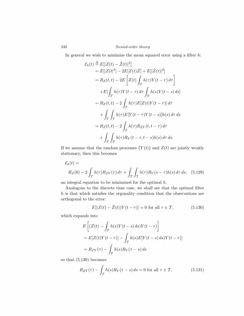
348 Second-order theory

In general we wish to minimize the mean squared error using a filter h:

Eh(t)∆= E[|Z(t) − Z(t)|2]= E[|Z(t|2] − 2E[Z(t)Z ] + E[|Z(t)|2]

= RZ(t, t) − 2E

[Z(t)

∫

Th(τ)Y (t − τ) dτ

]

+E[

∫

Th(τ)Y (t − τ) dτ

∫

Th(s)Y (t − s) ds]

= RZ(t, t) − 2

∫

Th(τ)E[Z(t)Y (t − τ)] dτ

+

∫

T

∫

Th(τ)E[Y (t − τ)Y (t − s)]h(s) dτ ds

= RZ(t, t) − 2

∫

Th(τ)RZY (t, t − τ) dτ

+

∫

T

∫

Th(τ)RY (t − τ, t − s)h(s) dτ ds.

If we assume that the random processes Y (t) and Z(t) are jointly weakly

stationary, then this becomes

Eh(t) =

RZ(0) − 2

∫

Th(τ)RZY (τ) dτ +

∫

T

∫

Th(τ)RY (s − τ)h(s) dτ ds, (5.129)

an integral equation to be minimized for the optimal h.

Analogous to the discrete time case, we shall see that the optimal filter

h is that which satisfies the orgonality condition that the observations are

orthogonal to the error:

E[(Z(t) − Z(t))Y (t − τ)] = 0 for all τ ∈ T , (5.130)

which expands into

E

[(Z(t) −

∫

Th(s)Y (t − s) ds)Y (t − τ)

]

= E[Z(t)Y (t − τ)] −∫

Th(s)E[Y (t − s) ds)Y (t − τ)]

= RZY (τ) −∫

Th(s)RY (τ − s) ds

so that (5.130) becomes

RZY (τ) −∫

Th(s)RY (τ − s) ds = 0 for all τ ∈ T , (5.131)

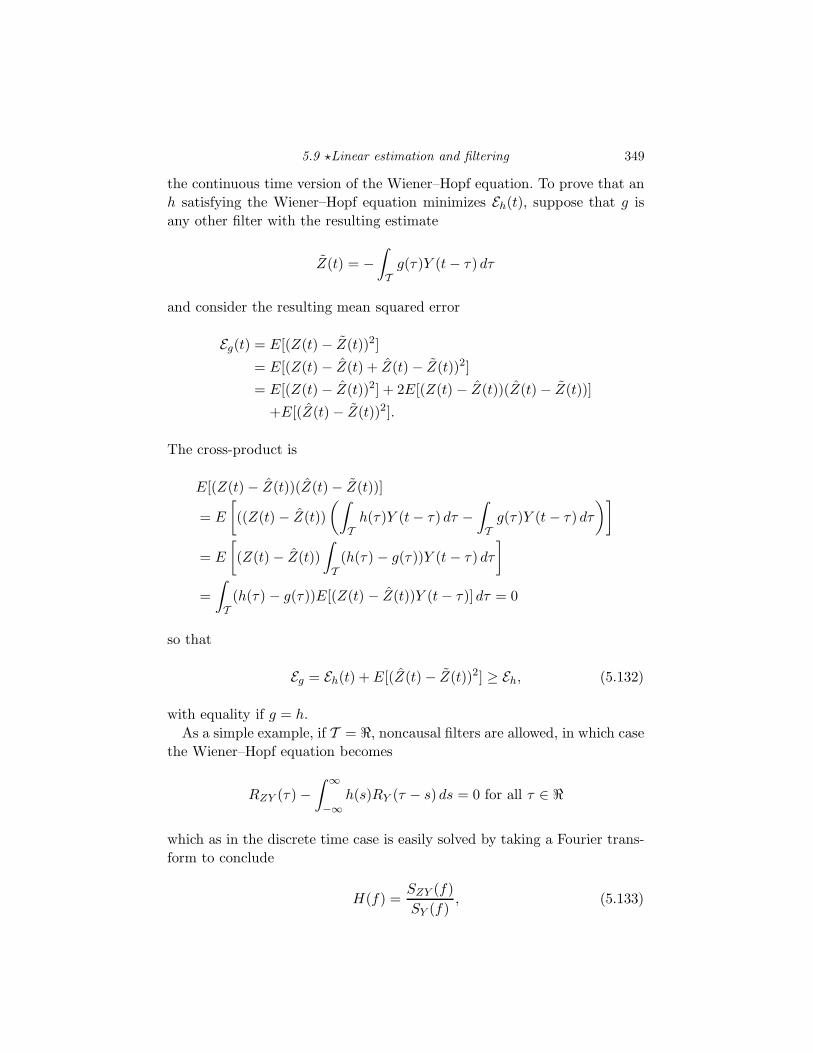
5.9 ⋆Linear estimation and filtering 349

the continuous time version of the Wiener–Hopf equation. To prove that an

h satisfying the Wiener–Hopf equation minimizes Eh(t), suppose that g is

any other filter with the resulting estimate

Z(t) = −∫

Tg(τ)Y (t − τ) dτ

and consider the resulting mean squared error

Eg(t) = E[(Z(t) − Z(t))2]

= E[(Z(t) − Z(t) + Z(t) − Z(t))2]

= E[(Z(t) − Z(t))2] + 2E[(Z(t) − Z(t))(Z(t) − Z(t))]

+E[(Z(t) − Z(t))2].

The cross-product is

E[(Z(t) − Z(t))(Z(t) − Z(t))]

= E

[((Z(t) − Z(t))

(∫

Th(τ)Y (t − τ) dτ −

∫

Tg(τ)Y (t − τ) dτ

)]

= E

[(Z(t) − Z(t))

∫

T(h(τ) − g(τ))Y (t − τ) dτ

]

=

∫

T(h(τ) − g(τ))E[(Z(t) − Z(t))Y (t − τ)] dτ = 0

so that

Eg = Eh(t) + E[(Z(t) − Z(t))2] ≥ Eh, (5.132)

with equality if g = h.

As a simple example, if T = ℜ, noncausal filters are allowed, in which case

the Wiener–Hopf equation becomes

RZY (τ) −∫ ∞

−∞h(s)RY (τ − s) ds = 0 for all τ ∈ ℜ

which as in the discrete time case is easily solved by taking a Fourier trans-

form to conclude

H(f) =SZY (f)

SY (f), (5.133)

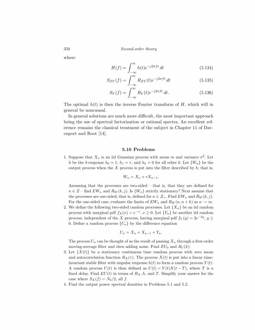
350 Second-order theory

where

H(f) =

∫ ∞

−∞h(t)e−j2πft dt (5.134)

SZY (f) =

∫ ∞

−∞RZY (t)e−j2πft dt (5.135)

SY (f) =

∫ ∞

−∞RY (t)e−j2πft dt. (5.136)

The optimal h(t) is then the inverse Fourier transform of H, which will in

general be noncausal.

In general solutions are much more difficult, the most important approach

being the use of spectral factorization or rational spectra. An excellent ref-

erence remains the classical treatment of the subject in Chapter 11 of Dav-

enport and Root [14].

5.10 Problems

1. Suppose that Xn is an iid Gaussian process with mean m and variance σ2. Let

h be the δ-response h0 = 1, h1 = r, and hk = 0 for all other k. Let Wn be the

output process when the X process is put into the filter described by h; that is,

Wn = Xn + rXn−1.

Assuming that the processes are two-sided – that is, that they are defined for

n ∈ Z – find EWn and RW (k, j). Is Wn strictly stationary? Next assume that

the processes are one-sided; that is, defined for n ∈ Z+. Find EWn and RW (k, j).

For the one-sided case, evaluate the limits of EWn and RW (n, n + k) as n → ∞.

2. We define the following two-sided random processes. Let Xn be an iid random

process with marginal pdf fX(x) = e−x, x ≥ 0. Let Yn be another iid random

process, independent of the X process, having marginal pdf fY (y) = 2e−2y, y ≥0. Define a random process Un by the difference equation

Un = Xn + Xn−1 + Yn.

The process Un can be thought of as the result of passing Xn through a first-order

moving-average filter and then adding noise. Find EU0 and RU (k).

3. Let X(t) be a stationary continuous time random process with zero mean

and autocorrelation function RX(τ). The process X(t) is put into a linear time-

invariant stable filter with impulse response h(t) to form a random process Y (t).

A random process U(t) is then defined as U(t) = Y (t)X(t − T ), where T is a

fixed delay. Find EU(t) in terms of RX , h, and T . Simplify your answer for the

case where SX(f) = N0/2, all f .

4. Find the output power spectral densities in Problems 5.1 and 5.2.

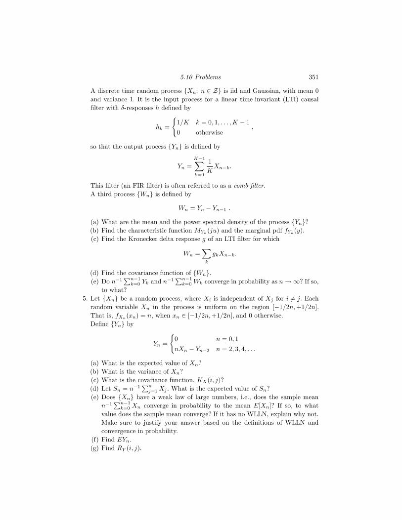
5.10 Problems 351

A discrete time random process Xn; n ∈ Z is iid and Gaussian, with mean 0

and variance 1. It is the input process for a linear time-invariant (LTI) causal

filter with δ-responses h defined by

hk =

1/K k = 0, 1, . . . , K − 1

0 otherwise,

so that the output process Yn is defined by

Yn =

K−1∑

k=0

1

KXn−k.

This filter (an FIR filter) is often referred to as a comb filter.

A third process Wn is defined by

Wn = Yn − Yn−1 .

(a) What are the mean and the power spectral density of the process Yn?(b) Find the characteristic function MYn

(ju) and the marginal pdf fYn(y).

(c) Find the Kronecker delta response g of an LTI filter for which

Wn =∑

k

gkXn−k.

(d) Find the covariance function of Wn.(e) Do n−1

∑n−1k=0 Yk and n−1

∑n−1k=0 Wk converge in probability as n → ∞? If so,

to what?

5. Let Xn be a random process, where Xi is independent of Xj for i 6= j. Each

random variable Xn in the process is uniform on the region [−1/2n, +1/2n].

That is, fXn(xn) = n, when xn ∈ [−1/2n, +1/2n], and 0 otherwise.

Define Yn by

Yn =

0 n = 0, 1

nXn − Yn−2 n = 2, 3, 4, . . .

(a) What is the expected value of Xn?

(b) What is the variance of Xn?

(c) What is the covariance function, KX(i, j)?

(d) Let Sn = n−1∑n

j=1 Xj . What is the expected value of Sn?

(e) Does Xn have a weak law of large numbers, i.e., does the sample mean

n−1∑n−1

k=0 Xn converge in probability to the mean E[Xn]? If so, to what

value does the sample mean converge? If it has no WLLN, explain why not.

Make sure to justify your answer based on the definitions of WLLN and

convergence in probability.

(f) Find EYn.

(g) Find RY (i, j).

352 Second-order theory

(h) Find the cdf of Y4 + Y6.

6. Let X(t); t ∈ ℜ be a stationary continuous time Gaussian random process

with zero mean and power spectral density function

SX(f) =

γ/2 0 ≤ |f | ≤ W

0 W < |f | < ∞.

Let Z(t); t ∈ ℜ be a stationary continuous time Gaussian random process with

zero mean and power spectral density function

SZ(f) =

N0/2 0 ≤ |f | ≤ B

0 B < |f | < ∞

where we assume that B >> W , γ > N0, and that the two processes are mutually

independent. We consider X(t) to be the “signal” and Z(t) to be the “noise.”

The receiver observes the process Y (t), where

Y (t) = X(t) + Z(t).

(a) Find and sketch the power spectral density of Y (t).(b) Find the conditional pdf fY (t)|X(t)(y|x), the marginal pdf fY (t)(y), and the

conditional pdf fX(t)|Y (t)(x|y).

(c) Find the minimum mean squared estimate X(t) given the single observation

Y (t) and compute the resulting mean squared error

ǫ2 = E[(X(t) − X(t))2].

(d) Suppose that you are allowed to use the entire observed signal Y (t) to

estimate X(t) at a specific time and you can do this by linearly filtering the

observed process. Suppose in particular that you pass the observed process

Y (t) through a linear filter with a transfer function

H(f) =

1 0 ≤ |f | ≤ W

0 W < |f | < ∞

with output X(t), an estimate of X(t). (This filter is not causal, but all the

results we derived for second-order input/output relations hold for noncausal

filters as well and can be used here.)

Find the resulting mean squared error E[(X(t) − X(t))2].

Which scheme yields smaller average mean squared error?

Hint: convince yourself that linearity implies that X(t) can be expressed as

X(t) plus the output of the filter H when the input is Z(t).

7. Let Xn be an iid Gaussian random process with zero mean and variance

RX(0) = σ2. Let Un be an iid binary random process, independent of the

X process, with Pr(Un = 1) = Pr(Un = −1) = 1/2. (All processes are assumed

to be two-sided in this problem.) Define the random process Zn = XnUn,

5.10 Problems 353

Yn = Un + Xn, and Wn = U0 + Xn, all n. Find the mean, covariance, and power

spectral density of each of these processes. Find the cross-covariance functions

between the processes.

8. Let Un, Xn, and Yn be the same as in Problem 5.7. The process Yn can

be viewed as a binary signal corrupted by additive Gaussian noise. One possible

method of trying to remove the noise at a receiver is to quantize the received Yn

to form an estimate Un = q(Yn) of the original binary sample, where

q(r) =

+1 if r ≥ 0

−1 if r < 0.

Write an integral expression for the error probability Pe = Pr(Un 6= Un). Find

the mean, covariance, and power spectral density of the Un process. Are the

processes Un and Un equivalent – that is, do they have the same process

distributions? Define an error process ǫn by ǫn = 0 if Un = Un and ǫn = 1 if

Un 6= Un. Find the marginal pmf, mean, covariance, and power spectral density

of the error process.

9. Cascade filters. Let gk and ak be the δ-responses of two discrete time causal

linear filters (gk = ak = 0 for k < 0) and let G(f) and A(f) be the corresponding

transfer functions, e.g.,

G(f) =

∞∑

k=0

gke−j2πkf .

Assume that g0 = a0 = 1. Let Zn be a weakly stationary uncorrelated random

process with variance σ2 and zero mean. Consider the cascade of two filters

formed by first putting an input Zn into the filter g to form the process Xn,

which is in turn put into the filter a to form the output process Yn.

(a) Let dk denote the δ-response of the overall cascade filter, that is,

Yn =

∞∑

k=0

dkZn−1.

Find an expression for dk in terms of gk and ak. As a check on your

answer you should have d0 = g0a0 = 1.

(b) Let D(f) be the transfer function of the cascade filter. Find D(f) in terms

of G(f) and A(f).

(c) Find the power spectral density SY (f) in terms of σ2, G, and A.

(d) Prove that

E(Y 2

n

)=

∫ 1/2

−1/2

SY (f)df ≥ σ2.

354 Second-order theory

Hint: show that if d0 = 1 (from part (a)), then

∫ 1/2

−1/2

|D(f)|2 df = 1 +

∫ 1/2

−1/2

|1 − D(f)|2 df ≥ 1.

10. One-step prediction. This problem develops a basic result of estimation theory.

No prior knowledge of estimation theory is required. Results from Problem 5.9

may be quoted without proof (even if you did not complete it). Let Xn be

as in problem 5.9; that is, it is a discrete time zero-mean random process with

power spectral density σ2|G(f)|2, where G(f) is the transfer function of a causal

filter with δ-response gk with g0 = 1. Form the process Xn by putting Xn

into a causal linear time-invariant filter with δ-response hk

Xn =

∞∑

k=1

hkXn−k.

Suppose that the linear filter tries to estimate the value of Xn based on the

values of Xi for all i < n by choosing the δ-response hk optimally. That is, the

filter estimates the next sample based on the present value and the entire past.

Such a filter is called a one-step predictor. Define the error process ǫn by

ǫn = Xn − Xn.

(a) Find expressions for the power spectral density Sǫ(f) in terms of SX(f) and

H(f). Use this result to evaluate Eǫ2n.

(b) Evaluate Sǫ(f) and E(ǫ2n) for the case where 1 − H(f) = 1/G(f).

(c) Use part (d) of Problem 5.9 to show that the prediction filter H(f) of (b)

in this problem yields the smallest possible value of E(ǫ2n) for any prediction

filter. You have just developed the optimal one-step prediction filter for the

case of a process that can be modeled as a weakly stationary uncorrelated

sequence passed through a linear filter. As discussed in the text, most discrete

time random processes can be modeled in such a fashion, at least through

second-order properties.

(d) Spectral factorization. Suppose that Xn has a power spectral density SX(f)

that satisfies∫ 1/2

−1/2

lnSX(f) df < ∞.

Expand lnSX(f) in a Fourier series and write the expression for

exp (lnSX(f)) in terms of the series to find G(f). Find the δ-response of

the optimum prediction filter in terms of your result. Find the mean square

error. (Hint: you will need to know what evenness of SX(f) implies for the co-

efficients in the requested series and what the Taylor series of an exponential

is.)

11. Binary filters. All of the linear filters considered so far were linear in the sense

5.10 Problems 355

of real arithmetic. It is sometimes useful to consider filters that are linear in

other algebraic systems, e.g., in binary or modulo 2 arithmetic as defined in

(3.64)–(3.65). Such systems are more appropriate, for example, when consider-

ing communications systems involving only binary arithmetic, such as binary

codes for noise immunity on digital communication links. A binary first-order

autoregressive filter with input process Xn and output process Yn is defined

by the difference equation

Yn = Yn−1 ⊕ Xn, all n.

Assume that the Xn is a Bernoulli process with parameter p. In this case the

process Yn is called a binary first-order autoregressive source.

(a) Show that for nonnegative integers k, the autocorrelation function of the

process Yn satisfies

RY (k) = E(YjYj+k) =1

2Pr

(k∑

i=1

Xi = an even number

).

(b) Use the result of (a) to evaluate RY and KY . Hint: this is most easily done

using a trick. Define the random variable

Wk =k∑

i=1

Xi.

This is a binomial random variable. Use this fact and the binomial theorem

to show that

Pr(Wk is odd) − Pr(Wk is even) = −(1 − 2p)k.

Alternatively, find a linear recursion relation for pk = Pr(Wk is odd) using

conditional probability (i.e., find a formula giving pk in terms of pk−1) and

then solve for pk.

(c) Find the power spectral density of the process Yn.12. Let Xn be a Bernoulli random process with parameter p and let ⊕ denote mod

2 addition as considered in Problem 5.11. Define the first-order binary moving-

average process Wn by the difference equation

Wn = Xn ⊕ Xn−1.

This is a mod 2 convolution and an example of what is called a convolutional

code in communication and information theory. Find pWn(w) and RW (k, j). Find

the power spectral density of the process Wn.13. Let X(t) be a continuous time zero-mean Gaussian random process with spec-

tral density SX(f) = N0/2, all f . Let H(f) and G(f) be the transfer functions

of two linear time-invariant filters with impulse responses h(t) and g(t), respec-

tively. The process X(t) is passed through the filter h(t) to obtain a process

356 Second-order theory

Y (t) and is also passed through the filter g(t) to obtain a process V (t); that

is,

Y (t) =

∫ ∞

0

h(τ)X(t − τ)dτ,

V (t) =

∫ ∞

0

g(τ)X(t − τ)dτ.

(a) Find the cross-correlation function RY,V (t, s) = E(YtVs).

(b) Under what assumptions on H and G are Yt and Vt independent random

variables?

14. Let X(t) and Y (t) be two continuous time zero-mean stationary Gaussian

processes with a common autocorrelation function R(τ) and common power spec-

tral densities S(f). Assume that X(t) and Y (t) are independent for all t, s. As-

sume also that E[X(t)Y (s)] = 0 all t, s and that σ2 = R(0). For a fixed frequency

f0, define the random process

W (t) = X(t) cos(2πf0t) + Y (t) sin(2πf0t).

Find the mean E(W (t)) and autocorrelation RW (t, s). Is W (t) weakly station-

ary?

15. Say that we are given an iid binary random process Xn with alphabet ±1, each

having probability one/2. We form a continuous time random process X(t) by

assigning

X(t) = Xn; t ∈ [(n − 1), nT ),

for a fixed time T . This process can also be described as follows: let p(t) be a

pulse that is 1 for t ∈ [0, T ) and 0 elsewhere. Define

X(t) =∑

k

Xkp(t − kT ).

This is an example of pulse amplitude modulation (PAM). If the process X(t)

is then used to phase-modulate a carrier, the resulting process is called a phase-

shift-keyed (PSK) modulation of the carrier by the process X(t). PSK is a

popular technique for digital communications. Define the PSK process

U(t) = a0 cos(2πf0t + δX(t)).

Observe that neither of these processes is stationary, but we can force them to

be at least weakly stationary by the trick of inserting uniform random variables

in appropriate places. Let Z be a random variable, uniformly distributed [0, T ]

and independent of the original iid process. Define the random process

Y (t) = X(t + Z).

Let Θ be a random variable uniformly distributed on [0, 1/f0] and independent

5.10 Problems 357

of Z and of the original iid random process. Define the process

V (t) = U(t + Θ).

Find the mean and autocorrelation functions of the processes Y (t) and V (t).16. Let X(t) be a Gaussian random process with zero mean and autocorrelation

function

RX(τ) =N0

2e−|τ |.

Find the power spectral density of the process. Let Y (t) be the process formed

by DSB-SC modulation of X(t). Letting Θ be uniformly distributed in (5.37),

sketch the lower spectral density of the modulated process.

17. A continuous time two-sided weakly stationary Gaussian random process S(t)with zero mean and power spectral density SS(f) is put into a noisy communi-

cation channel. First, white Gaussian noise W (t) with power spectral density

N0/2 is added, where the two random processes are assumed to be independent

of one another, and then the sum S(t) + W (t) is passed through a linear fil-

ter with impulse response h(t) and transfer function H(f) to form a received

process Y (t). Find an expression for the power spectral density SY (f). Find

an expression for the expected square error E[(S(t) − Y (t))2] and the so-called

signal-to-noise ratio (SNR)

E(S(t)2)

E[(S(t) − Y (t))2].

Suppose that you know that SY (f) can be factored into the form |G(f)|2, where

G(f) is a stable causal filter with a stable causal inverse. What is the best choice

of H(f) in the sense of maximizing the signal-to-noise ratio? What is the best

causal H(f)?

18. Show that (5.2) converges in mean square if the filter is stable and the input

process has finitely bounded mean and variance. Show that convergence with

probability one is achieved if the convergence of (A.43) is fast enough for the

δ-response.

19. Show that the sum of equation (5.7) converges for the two-sided weakly sta-

tionary case if the filter is stable and the input process has finitely bounded

variance.

20. Equation (5.79) shows how the power spectral density is affected by differentia-

tion of a process. Provide a formal argument for the integration counterpart of

this result; that is, if X(t) is a stationary two-sided continuous time random

process and Y (t) =∫ t

−∞ X(s) dx, then, subject to suitable technical conditions,

SY (f) = SX(f)/f2.

21. Prove that (5.115) holds under the conditions given.

22. Suppose that YN is as in Example [5.1] and that Wn = Yn + Un, where Un is

a zero-mean white noise process with second moment E(U2) = N0/2. Solve the

358 Second-order theory

Wiener–Hopf equation to obtain a LLSE of Yn+m given Wi; i ≤ n for m > n.

Evaluate the resulting mean squared error.

23. Prove the claim that if Xn and Yn are described by (5.116) and (5.117) and

if Xn is a LLSE estimate of Xn given the previous n samples Y0, Y1, . . . , Yn−1,

then Yn = HnXn is a LLSE estimate of Yn given the same observations.

24. Prove the claim that the innovations sequence νn of Example [5.7] is uncor-

related and has zero mean. (Fill in the details of the arguments used in the

text.)

25. Let YN be as in Example [5.2]. Find the LLSE for Yn+m given Y0, Y1, . . . , Ynfor an arbitrary positive integer m. Evaluate the mean square error. Repeat for

the process of Example [5.3] (the same process with r = 1).

26. Specialize the recursive estimator formulas of (5.124) through (5.127) to the case

where Xn is the Yn process of Example [5.2], where Hn is a constant, say a,

and where Ψn − N0/2, all n. Describe the behavior of the estimator as n → ∞.

27. Find an expression for the mean square error in Example [5.4]. Specialize to

infinite smoothing.

28. In the section on linear estimation we assumed that all processes had zero-mean

functions. In this problem we remove this assumption. Let Xn and Yn be

random processes with mean functions mX(n) and mY (n), respectively. We

estimate Xn by adding a constant to (5.109); i.e.,

Xn = an +∑

k:n−k∈KhkYn−k.

(a) Show that the minimum mean square estimate of Xn is Xn = mX(n) if no

observations are used.

(b) Modify and prove Theorem 5.2 to allow for the nonzero means.

29. Suppose that Xn and Zn are zero-mean, mutually independent, iid, two-

sided Gaussian random processes with correlations

RX(k) = σ2xδk; RZ(k) = σ2

zδk;

These processes are used to construct new processes as follows:

Yn = Zn + rYn−1

Un = Xn + Zn

Wn = Un + rUn−1.

Find the covariance and power spectral densities of Un and Wn. Find

E[(Xn − Wn)2].

30. Suppose that Zn and Wn are two mutually independent two-sided zero-mean

iid Gaussian processes with variances σ2Z and σ2

W , respectively. Zn is put into a

linear time-invariant filter to form an output process Xn defined by

Xn = Zn − rZn−1,

5.10 Problems 359

where 0 < r < 1. (Such a filter is sometimes called a pre-emphasis filter in speech

processing.) This process is then used to form a new process

Yn = Xn + Wn,

which can be viewed as a noisy version of the pre-emphasized Zn process. Lastly,

the Yn process is put through a “de-emphasis filter” to form an output process

Un defined by

Un = rUn−1 + Yn.

(a) Find the autocorrelation RZ and the power spectral density SZ . Recall

that for a weakly stationary discrete time process with zero mean RZ(k) =

E(ZnZn+k) and

SZ(f) =

∞∑

k=−∞RZ(k)e−j2πfk,

the discrete time Fourier transform of RZ .

(b) Find the autocorrelation RX and the power spectral density SX .

(c) Find the autocorrelation RY and the power spectral density SY .

(d) Find the overall mean squared error E[(Un − Zn)2].

31. Suppose that Xn; n ∈ Z is a discrete time iid Gaussian random processes

with zero mean and variance σ2X = E[X2

0 ]. We consider this an input signal to a

signal processing system. Suppose also that Wn; n ∈ Z is a discrete time iid

Gaussian random processes with zero mean and variance σ2W and that the two

processes are mutually independent. We consider Wn to be noise. Suppose that

Xn is put into a linear filter with unit δ-response h, where

hk =

1 k = 0

−1 k = −1

0 otherwise

to form an output U = X ∗ h, the convolution of the input signal and the unit

δ-response. The final output signal is then formed by adding the noise to the

filtered input signal, Yn = Un + Wn.

(a) Find the mean, power spectral density, and marginal pdf for Un.

(b) Find the mean, covariance, and power spectral density for Yn.(c) Find E[YnXn].

(d) Does the mean ergodic theorem hold for Yn?32. Suppose that X(t); t ∈ R is a weakly stationary continuous time Gaussian

random process with zero mean and autocorrelation function

RX(τ) = E[X(t)X(t + τ)] = σ2Xe−|τ |.

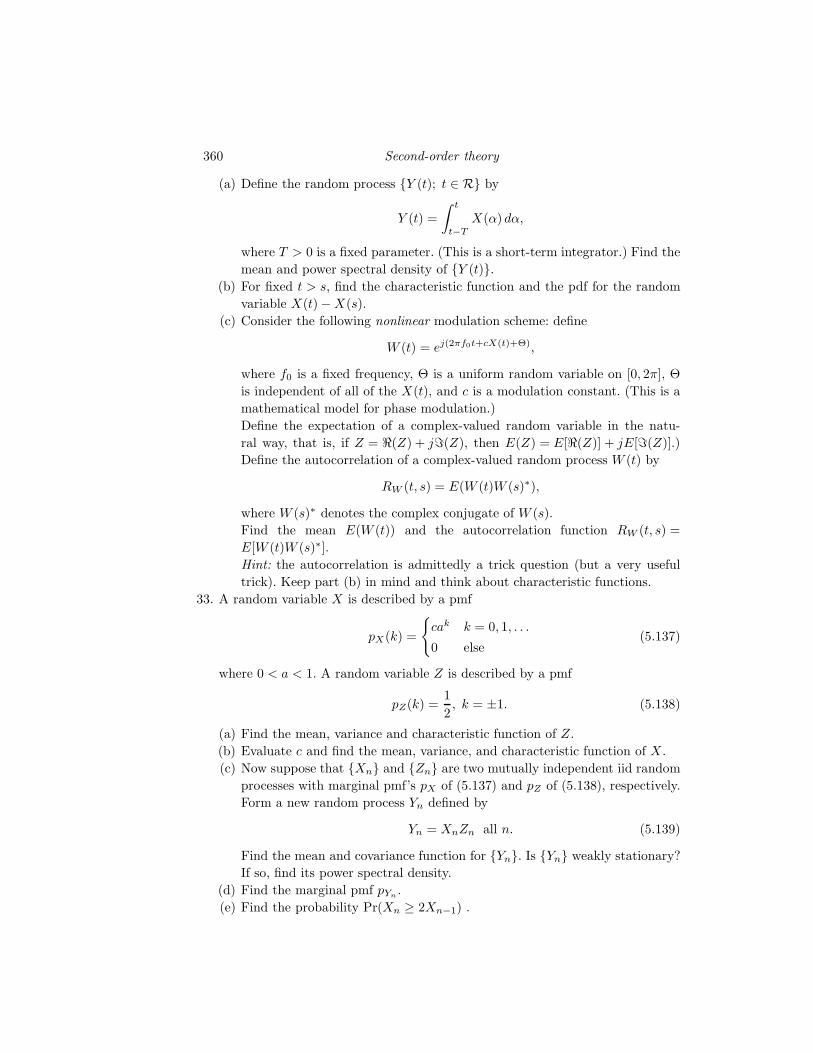
360 Second-order theory

(a) Define the random process Y (t); t ∈ R by

Y (t) =

∫ t

t−T

X(α) dα,

where T > 0 is a fixed parameter. (This is a short-term integrator.) Find the

mean and power spectral density of Y (t).(b) For fixed t > s, find the characteristic function and the pdf for the random

variable X(t) − X(s).

(c) Consider the following nonlinear modulation scheme: define

W (t) = ej(2πf0t+cX(t)+Θ),

where f0 is a fixed frequency, Θ is a uniform random variable on [0, 2π], Θ

is independent of all of the X(t), and c is a modulation constant. (This is a

mathematical model for phase modulation.)

Define the expectation of a complex-valued random variable in the natu-

ral way, that is, if Z = ℜ(Z) + jℑ(Z), then E(Z) = E[ℜ(Z)] + jE[ℑ(Z)].)

Define the autocorrelation of a complex-valued random process W (t) by

RW (t, s) = E(W (t)W (s)∗),

where W (s)∗ denotes the complex conjugate of W (s).

Find the mean E(W (t)) and the autocorrelation function RW (t, s) =

E[W (t)W (s)∗].Hint: the autocorrelation is admittedly a trick question (but a very useful

trick). Keep part (b) in mind and think about characteristic functions.

33. A random variable X is described by a pmf

pX(k) =

cak k = 0, 1, . . .

0 else(5.137)

where 0 < a < 1. A random variable Z is described by a pmf

pZ(k) =1

2, k = ±1. (5.138)

(a) Find the mean, variance and characteristic function of Z.

(b) Evaluate c and find the mean, variance, and characteristic function of X .

(c) Now suppose that Xn and Zn are two mutually independent iid random

processes with marginal pmf’s pX of (5.137) and pZ of (5.138), respectively.

Form a new random process Yn defined by

Yn = XnZn all n. (5.139)

Find the mean and covariance function for Yn. Is Yn weakly stationary?

If so, find its power spectral density.

(d) Find the marginal pmf pYn.

(e) Find the probability Pr(Xn ≥ 2Xn−1) .

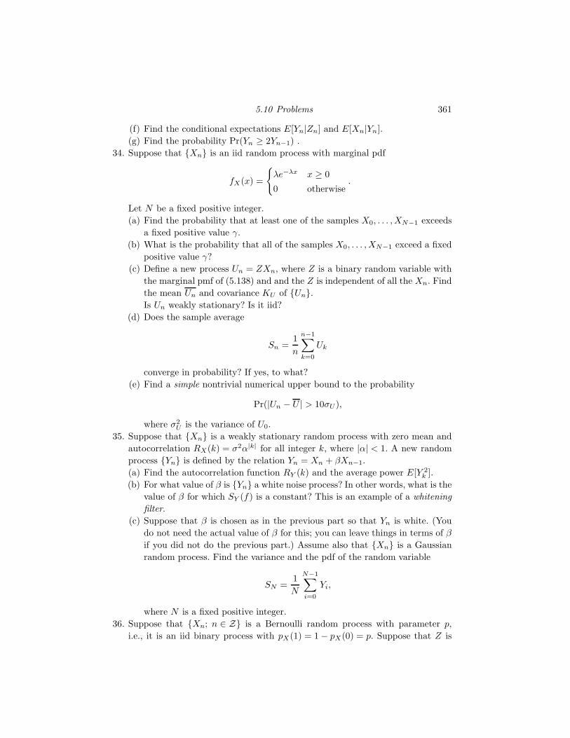
5.10 Problems 361

(f) Find the conditional expectations E[Yn|Zn] and E[Xn|Yn].

(g) Find the probability Pr(Yn ≥ 2Yn−1) .

34. Suppose that Xn is an iid random process with marginal pdf

fX(x) =

λe−λx x ≥ 0

0 otherwise.

Let N be a fixed positive integer.

(a) Find the probability that at least one of the samples X0, . . . , XN−1 exceeds

a fixed positive value γ.

(b) What is the probability that all of the samples X0, . . . , XN−1 exceed a fixed

positive value γ?

(c) Define a new process Un = ZXn, where Z is a binary random variable with

the marginal pmf of (5.138) and and the Z is independent of all the Xn. Find

the mean Un and covariance KU of Un.Is Un weakly stationary? Is it iid?

(d) Does the sample average

Sn =1

n

n−1∑

k=0

Uk

converge in probability? If yes, to what?

(e) Find a simple nontrivial numerical upper bound to the probability

Pr(|Un − U | > 10σU ),

where σ2U is the variance of U0.

35. Suppose that Xn is a weakly stationary random process with zero mean and

autocorrelation RX(k) = σ2α|k| for all integer k, where |α| < 1. A new random

process Yn is defined by the relation Yn = Xn + βXn−1.

(a) Find the autocorrelation function RY (k) and the average power E[Y 2k ].

(b) For what value of β is Yn a white noise process? In other words, what is the

value of β for which SY (f) is a constant? This is an example of a whitening

filter.

(c) Suppose that β is chosen as in the previous part so that Yn is white. (You

do not need the actual value of β for this; you can leave things in terms of β

if you did not do the previous part.) Assume also that Xn is a Gaussian

random process. Find the variance and the pdf of the random variable

SN =1

N

N−1∑

i=0

Yi,

where N is a fixed positive integer.

36. Suppose that Xn; n ∈ Z is a Bernoulli random process with parameter p,

i.e., it is an iid binary process with pX(1) = 1 − pX(0) = p. Suppose that Z is

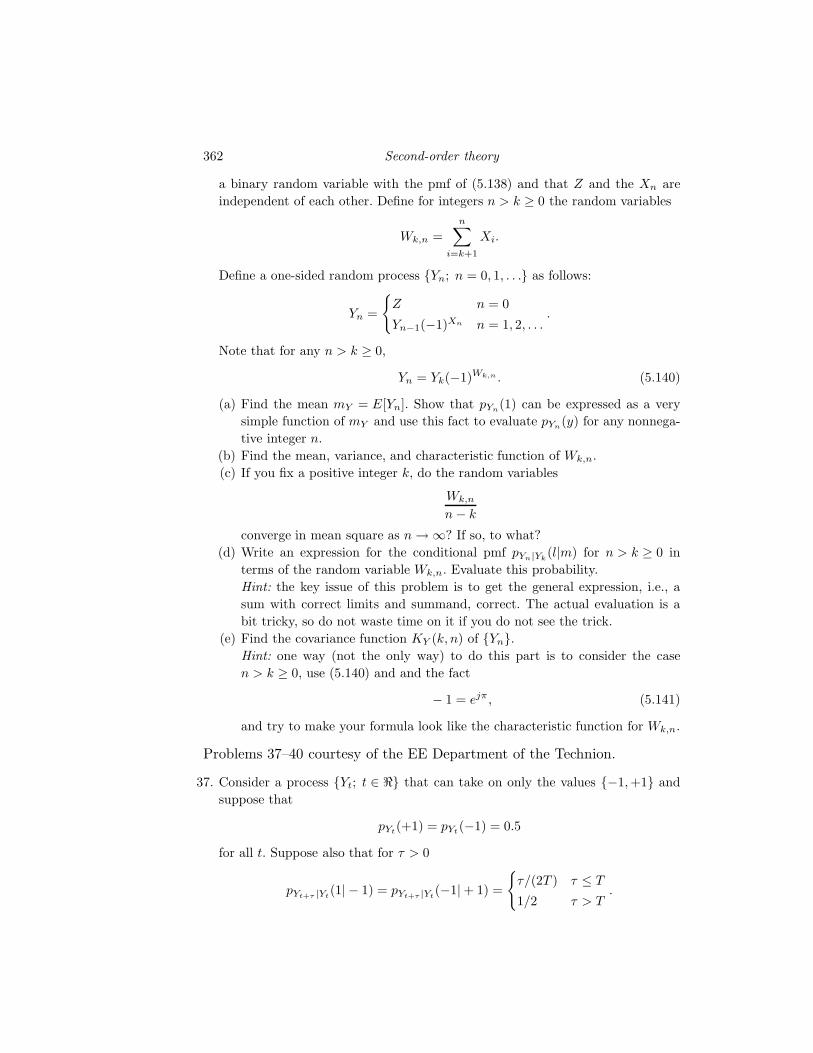
362 Second-order theory

a binary random variable with the pmf of (5.138) and that Z and the Xn are

independent of each other. Define for integers n > k ≥ 0 the random variables

Wk,n =

n∑

i=k+1

Xi.

Define a one-sided random process Yn; n = 0, 1, . . . as follows:

Yn =

Z n = 0

Yn−1(−1)Xn n = 1, 2, . . ..

Note that for any n > k ≥ 0,

Yn = Yk(−1)Wk,n . (5.140)

(a) Find the mean mY = E[Yn]. Show that pYn(1) can be expressed as a very

simple function of mY and use this fact to evaluate pYn(y) for any nonnega-

tive integer n.

(b) Find the mean, variance, and characteristic function of Wk,n.

(c) If you fix a positive integer k, do the random variables

Wk,n

n − k

converge in mean square as n → ∞? If so, to what?

(d) Write an expression for the conditional pmf pYn|Yk(l|m) for n > k ≥ 0 in

terms of the random variable Wk,n. Evaluate this probability.

Hint: the key issue of this problem is to get the general expression, i.e., a

sum with correct limits and summand, correct. The actual evaluation is a

bit tricky, so do not waste time on it if you do not see the trick.

(e) Find the covariance function KY (k, n) of Yn.Hint: one way (not the only way) to do this part is to consider the case

n > k ≥ 0, use (5.140) and and the fact

− 1 = ejπ , (5.141)

and try to make your formula look like the characteristic function for Wk,n.

Problems 37–40 courtesy of the EE Department of the Technion.

37. Consider a process Yt; t ∈ ℜ that can take on only the values −1, +1 and

suppose that

pYt(+1) = pYt

(−1) = 0.5

for all t. Suppose also that for τ > 0

pYt+τ |Yt(1| − 1) = pYt+τ |Yt

(−1| + 1) =

τ/(2T ) τ ≤ T

1/2 τ > T.

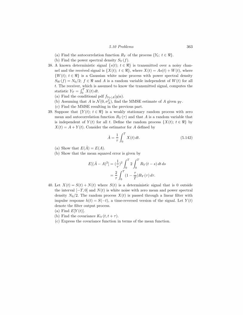
5.10 Problems 363

(a) Find the autocorrelation function RY of the process Yt; t ∈ ℜ.(b) Find the power spectral density SY (f).

38. A known deterministic signal s(t); t ∈ ℜ is transmitted over a noisy chan-

nel and the received signal is X(t); t ∈ ℜ, where X(t) = As(t) + W (t), where

W (t); t ∈ ℜ is a Gaussian white noise process with power spectral density

SW (f) = N0/2; f ∈ ℜ and A is a random variable independent of W (t) for all

t. The receiver, which is assumed to know the transmitted signal, computes the

statistic YT =∫ T

0 X(t) dt.

(a) Find the conditional pdf fYT |A(y|a).

(b) Assuming that A is N (0, σ2A), find the MMSE estimate of A given yT .

(c) Find the MMSE resulting in the previous part.

39. Suppose that Y (t); t ∈ ℜ is a weakly stationary random process with zero

mean and autocorrelation function RY (τ) and that A is a random variable that

is independent of Y (t) for all t. Define the random process X(t); t ∈ ℜ by

X(t) = A + Y (t). Consider the estimator for A defined by

A =1

τ

∫ T

0

X(t) dt. (5.142)

(a) Show that E(A) = E(A).

(b) Show that the mean squared error is given by

E[(A − A)2] = (1

τ)2∫ T

0

2

∫ T

0

RY (t − s) dt ds

=2

τ

∫ T

0

(1 − τ

T)RY (τ) dτ.

40. Let X(t) = S(t) + N(t) where S(t) is a deterministic signal that is 0 outside

the interval [−T, 0] and N(t) is white noise with zero mean and power spectral

density N0/2. The random process X(t) is passed through a linear filter with

impulse response h(t) = S(−t), a time-reversed version of the signal. Let Y (t)

denote the filter output process.

(a) Find E[Y (t)].

(b) Find the covariance KY (t, t + τ).

(c) Express the covariance function in terms of the mean function.

6

A menagerie of processes

The basic tools for describing and analyzing random processes have all been

developed in the preceding chapters along with a variety of examples of ran-

dom processes with and without memory. The goal of this chapter is to use

these tools to describe a menagerie of useful random processes, usually by

taking a simple random process and applying some form of signal process-

ing such as linear filtering in order to produce a more complicated random

process. In Chapter 5 the effect of linear filtering on second-order moments

was considered. In this chapter we look in more detail at the resulting out-

put process and consider other forms of signal processing as well. In the

course of the development a few new tools and several variations on old

tools for deriving distributions are introduced. Much of this chapter can be

considered as practice of the methods developed in the previous chapters,

with names often being given to the specific examples developed. In fact

several processes with memory have been encountered previously: the bino-

mial counting process and the discrete time Wiener process, in particular.

The goal now is to extend the techniques used in these special cases to more

general situations and to introduce a wider variety of processes.

The development of examples begins with a continuation of the study of

the output processes of linear systems with random process inputs. The goal

is to develop the detailed structure of such processes and of other processes

with similar behavior that cannot be described by a linear system model. In

Chapter 5, we confined interest to second-order properties of the output ran-

dom process, properties that can be found under quite general assumptions

about the input process and filter. In order to get more detailed probabilis-

tic descriptions of the output process, in this chapter we restrict the input

process for the discrete time case to be an iid random process and study the

resulting output process and the continuous time analog to such a process.

By restricting the structure of the output process in this manner, we shall see

364

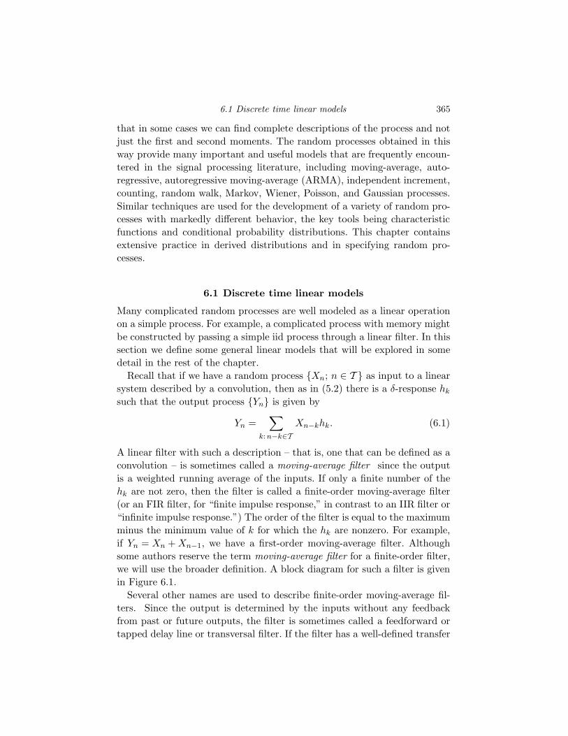
6.1 Discrete time linear models 365

that in some cases we can find complete descriptions of the process and not

just the first and second moments. The random processes obtained in this

way provide many important and useful models that are frequently encoun-

tered in the signal processing literature, including moving-average, auto-

regressive, autoregressive moving-average (ARMA), independent increment,

counting, random walk, Markov, Wiener, Poisson, and Gaussian processes.

Similar techniques are used for the development of a variety of random pro-

cesses with markedly different behavior, the key tools being characteristic

functions and conditional probability distributions. This chapter contains

extensive practice in derived distributions and in specifying random pro-

cesses.

6.1 Discrete time linear models

Many complicated random processes are well modeled as a linear operation

on a simple process. For example, a complicated process with memory might

be constructed by passing a simple iid process through a linear filter. In this

section we define some general linear models that will be explored in some

detail in the rest of the chapter.

Recall that if we have a random process Xn; n ∈ T as input to a linear

system described by a convolution, then as in (5.2) there is a δ-response hk

such that the output process Yn is given by

Yn =∑

k:n−k∈TXn−khk. (6.1)

A linear filter with such a description – that is, one that can be defined as a

convolution – is sometimes called a moving-average filter since the output

is a weighted running average of the inputs. If only a finite number of the

hk are not zero, then the filter is called a finite-order moving-average filter

(or an FIR filter, for “finite impulse response,” in contrast to an IIR filter or

“infinite impulse response.”) The order of the filter is equal to the maximum

minus the minimum value of k for which the hk are nonzero. For example,

if Yn = Xn + Xn−1, we have a first-order moving-average filter. Although

some authors reserve the term moving-average filter for a finite-order filter,

we will use the broader definition. A block diagram for such a filter is given

in Figure 6.1.

Several other names are used to describe finite-order moving-average fil-

ters. Since the output is determined by the inputs without any feedback

from past or future outputs, the filter is sometimes called a feedforward or

tapped delay line or transversal filter. If the filter has a well-defined transfer

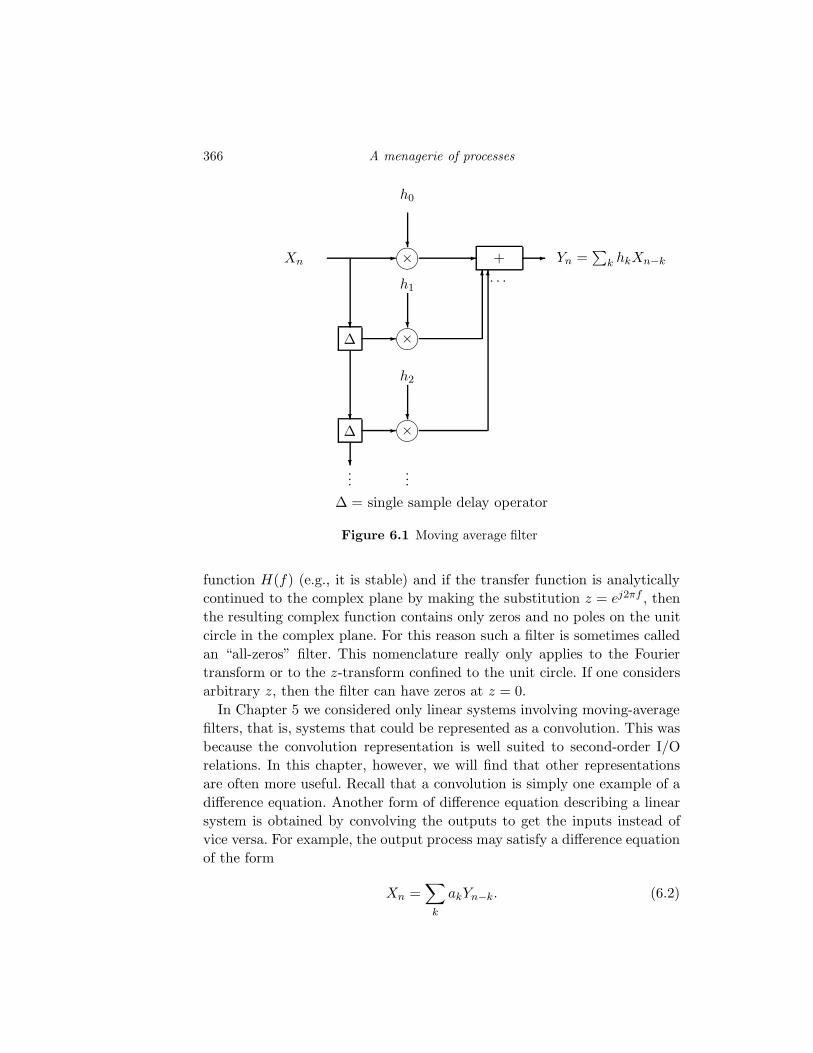
366 A menagerie of processes

Xn-

×?

h0

- + - Yn =∑

k hkXn−k

?∆ -

×?

h16

?∆ -

×?

h2

6

?...

...

· · ·

∆ = single sample delay operator

Figure 6.1 Moving average filter

function H(f) (e.g., it is stable) and if the transfer function is analytically

continued to the complex plane by making the substitution z = ej2πf , then

the resulting complex function contains only zeros and no poles on the unit

circle in the complex plane. For this reason such a filter is sometimes called

an “all-zeros” filter. This nomenclature really only applies to the Fourier

transform or to the z-transform confined to the unit circle. If one considers

arbitrary z, then the filter can have zeros at z = 0.

In Chapter 5 we considered only linear systems involving moving-average

filters, that is, systems that could be represented as a convolution. This was

because the convolution representation is well suited to second-order I/O

relations. In this chapter, however, we will find that other representations

are often more useful. Recall that a convolution is simply one example of a

difference equation. Another form of difference equation describing a linear

system is obtained by convolving the outputs to get the inputs instead of

vice versa. For example, the output process may satisfy a difference equation

of the form

Xn =∑

k

akYn−k. (6.2)

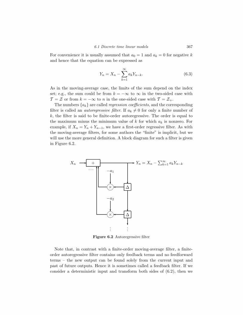
6.1 Discrete time linear models 367

For convenience it is usually assumed that a0 = 1 and ak = 0 for negative k

and hence that the equation can be expressed as

Yn = Xn −∞∑

k=1

akYn−k. (6.3)

As in the moving-average case, the limits of the sum depend on the index

set; e.g., the sum could be from k = −∞ to ∞ in the two-sided case with

T = Z or from k = −∞ to n in the one-sided case with T = Z+.

The numbers ak are called regression coefficients, and the corresponding

filter is called an autoregressive filter. If ak 6= 0 for only a finite number of

k, the filter is said to be finite-order autoregressive. The order is equal to

the maximum minus the minimum value of k for which ak is nonzero. For

example, if Xn = Yn + Yn−1, we have a first-order regressive filter. As with

the moving-average filters, for some authors the “finite” is implicit, but we

will use the more general definition. A block diagram for such a filter is given

in Figure 6.2.

Xn- + - Yn = Xn −∑∞

k=1 akYn−k

?∆

×?

−a16

?∆

×?

−a2

6

?...

...

· · ·

Figure 6.2 Autoregressive filter

Note that, in contrast with a finite-order moving-average filter, a finite-

order autoregressive filter contains only feedback terms and no feedforward

terms – the new output can be found solely from the current input and

past of future outputs. Hence it is sometimes called a feedback filter. If we

consider a deterministic input and transform both sides of (6.2), then we

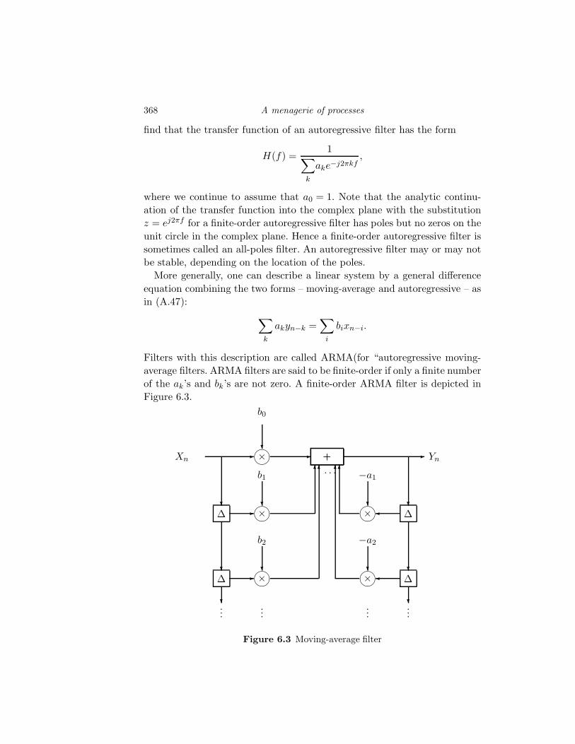
368 A menagerie of processes

find that the transfer function of an autoregressive filter has the form

H(f) =1∑

k

ake−j2πkf,

where we continue to assume that a0 = 1. Note that the analytic continu-

ation of the transfer function into the complex plane with the substitution

z = ej2πf for a finite-order autoregressive filter has poles but no zeros on the

unit circle in the complex plane. Hence a finite-order autoregressive filter is

sometimes called an all-poles filter. An autoregressive filter may or may not

be stable, depending on the location of the poles.

More generally, one can describe a linear system by a general difference

equation combining the two forms – moving-average and autoregressive – as

in (A.47):

∑

k

akyn−k =∑

i

bixn−i.

Filters with this description are called ARMA(for “autoregressive moving-

average filters. ARMA filters are said to be finite-order if only a finite number

of the ak’s and bk’s are not zero. A finite-order ARMA filter is depicted in

Figure 6.3.

Xn-

×?

b0

- +

?∆ -

×?

b16

?∆ -

×?

b2

6

?...

...

· · ·+ - Yn

?∆

×?

−a16

?∆

×?

−a2

6

?...

...

Figure 6.3 Moving-average filter

6.1 Discrete time linear models 369

Once again, it should be noted that some authors use finite-order implic-

itly, a convention that we will not adopt. Applying a deterministic input

and using (A.45), we find that the transfer function of an ARMA filter has

the form

H(f) =

∑

i

bie−j2πif

∑

k

ake−j2πkf, (6.4)

where we continue to assume that a0 = 1.

As we shall see by example, one can often describe a linear system by

any of these filters, and hence one often chooses the simplest model for

the desired application. For example, an ARMA filter representation with

only three nonzero ak and two nonzero bk would be simpler than either a

pure autoregressive or pure moving-average representation, which would in

general require an infinite number of parameters. The general development

of representations of one type of filter or process from another is an area of

complex analysis that is outside the scope of this book. We shall, however,

see some simple examples where different representations are easily found.

We are now ready to introduce three classes of random processes that

are collectively called linear models since they are formed by putting an iid

process into a linear system.

A discrete time random process Yn is called an autoregressive random

process if it is formed by putting an iid random process into an autoregressive

filter. Similarly, the process is said to be a moving-average random process

or ARMA random process if it is formed by putting an iid process into a

moving-average or ARMA filter, respectively. If a finite-order filter is used,

the order of the process is the same as the order of the filter.

Since iid processes are uncorrelated, the techniques of Chapter 5 imme-

diately yield the power spectral densities of these processes in the two-

sided weakly stationary case and yield in general the second-order moments

of moving-average processes. In fact, some books and papers which deal

only with second-order moment properties define an autoregressive (moving-

average, ARMA) process more generally as the output of an autoregressive

(moving-average, ARMA) filter with a weakly stationary uncorrelated input.

We use the stricter definition in order to derive actual distributions in addi-

tion to second-order moments. We shall see that we can easily find marginal

probability distributions for moving-average processes. Perhaps surprisingly,

however, the autoregressive models will prove to be much more useful for

finding more complete specifications, that is, joint probability distributions

370 A menagerie of processes

for the output process. The basic ideas are most easily demonstrated in the

simple, and familiar, Example [5.3], summing successive outputs of an iid

process.

6.2 Sums of iid random variables

We begin by recalling a simple but important example from Chapters 3

and 5 considered in examples [3.35], [3.37], and [5.3]. These examples can

be used to exemplify both autoregressive and moving-average filters. Let

Xn; n = 1, 2, . . . be an iid process with mean m and variance σ2 (with

discrete or continuous alphabet). Consider a linear filter with Kronecker

δ-response

hk =

1 k = 0, 1, 2 . . .

0 otherwise. (6.5)

This is the discrete time integrator and it is not stable. The output process

is then given as the sum of iid random variables:

Yn =

0 n = 0∑n

i=1 Xi n = 1, 2, . . .. (6.6)

The two best-known members of this class are the binomial counting process

and the Wiener process (or discrete time diffusion process), which were

encountered in Chapter 3

We have changed notation slightly from Example [5.3] since here we force

Y0 = 0. Observe that if we further let X0 = 0, then by definition Yn; n ∈Z+ is a moving-average random process by construction with the moving-

average filter hk = 1 for all nonnegative k.

Since an iid input process is also uncorrelated, we can apply example [5.3]

(with a slight change due to the different indexing) and evaluate the first

and second moments of the Y process as

EYn = mn; n = 1, 2, . . .

and

KY (k, j) = σ2 min(k, j); k, j = 1, 2, . . .

For later use we state these results in a slightly different notation: since

EY1 = m, since KY (1, 1) = σ2Y1

= σ2, and since the formulas also hold for

n = 0 and for k = j = 0, we have that

EYt = tEY1; t ≥ 0 (6.7)

6.3 Independent stationary increment processes 371

and

KY (t, s) = σ2Y1

min(t, s); t, s ≥ 0. (6.8)

We explicitly consider only those values of t and s that are in the appropriate

index set, here the nonnegative integers. An alternative representation to the

linear system representation defined by (3.136) is obtained by rewriting the

sum as a linear difference equation with initial conditions:

Yn =

0 n = 0

Yn−1 + Xn n = 1, 2, 3, . . .. (6.9)

Observe that in this guise, Yn is a first-order autoregressive process (see

(6.2)) since it is obtained by passing the iid X process through a first-order

autoregressive filter with a0 = 1 and a1 = −1. Observe again that this filter

is not stable, but it does have a transfer function, H(f) = 1/(1 − e−j2πf )

(which, with the substitution z = ej2πf , has a pole on the unit circle).

We have seen from Section 3.12 how to find the marginal distributions for

such sums of iid processes and have seen from Section 3.7 how to find the

conditional distributions and hence a complete specification. The natural

question at this point is how general the methods and results referred to

are. Toward this end we consider generalizations in several directions. First

we consider a direct generalization to continuous time processes, the class

of processes with independent and stationary increments. We next consider

partial generalizations to discrete time moving-average and autoregressive

processes.

6.3 Independent stationary increment processes

We now generalize the class of processes formed by summing iid random

variables in a way that works for both continuous and discrete time. The

generalization is accomplished by focusing on the changes in a process rather

than on the values of the process. The general class, that of processes with

independent and stationary increments, reduces in the discrete time case to

the class considered in the previous sections: processes formed by summing

outputs of an iid process.

The change in value of a random process in moving forward in any given

time interval is called a jump or increment of the process. The specific class of

processes that we now consider consists of random processes whose jumps or

increments in nonoverlapping time intervals are independent random vari-

ables whose probability distributions depend only on the time differences

372 A menagerie of processes

over which the jumps occur. In the discrete time case, the nth output of

such processes can be regarded as the sum of the first n random variables

produced by an iid random process. Because the jumps in nonoverlapping

time intervals then consist of sums of different iid random variables, the

jumps are obviously independent. This general class of processes is of in-

terest for three reasons. First, the class contains two of the most important

examples of random processes: the Wiener process and the Poisson counting

process. Second, members of the class form building blocks for many other

random process models. For example, in Chapter 5 we presented an intu-

itive derivation of the properties of continuous time Gaussian white noise.

A rigorous development would be based on the Wiener process, which we

can treat rigorously with elementary tools. Third, these processes provide a

useful vehicle for practice with several important and useful tools of probabil-

ity theory: characteristic functions, conditional pmf’s, conditional pdf’s, and

nonelementary conditional probability. In addition, independent increment

processes provide specific examples of several general classes of processes:

Markov processes, counting processes, and random walks.

Independent and stationary increment processes are generally not them-

selves weakly stationary since, as has already been seen in the discrete time

case, their probabilistic description changes with time. They possess, how-

ever, some stationarity properties. In particular the distributions of the

jumps or increments taken over fixed-length time intervals are stationary

even though the distributions of the process are not.

The increments or jumps or differences of a random process are obtained

by picking a collection of ordered sample times and forming the pairwise

differences of the samples of the process taken at these times. For example,

given a discrete time or continuous time random process Yt; t ∈ T , one

can choose a collection of sample times t0, t1, . . . , tk (ti ∈ T , all i) where we

assume that the sample times are ordered in the sense that

t0 < t1 < t2 < . . . < tk.

Given this collection of sample times, the corresponding increments of the

process Yt are the differences

Yti − Yti−1 ; i = 1, 2, . . . , k.

Note that the increments very much depend on the choice of the sample

times; one would expect quite different behavior when the samples are widely

separated than when they are nearby. We can now define the general class of

6.3 Independent stationary increment processes 373

processes with independent increments for both the discrete and continuous

time cases.

A random process Yt; t ∈ T is said to have independent increments or to

be an independent increment random process if for all choices of k and sample

times ti; i = 1, . . . , k, the increments Yti − Yti−1 ; i = 1, 2, . . . , k are inde-

pendent random variables. An independent increment process is said to have

stationary increments if the distribution of the increment Yt+δ − Ys+δ does

not depend on δ for all allowed values of t > s and δ. (Observe that this is

really only a first-order stationarity requirement on the increments, not by

definition a strict stationarity requirement, but the language is standard.

In any case, if the increments are independent and stationary in this sense,

then they are also strictly stationary.)

We shall call a random process an independent stationary increment or isi

process if it has independent and stationary increments.

We shall always make the additional assumption that 0 is the smallest

possible time index; that is, that t ≥ 0 for all t ∈ T , and that Y0 = 0 as in

the discrete time case. We shall see that such processes are not stationary

and that they must “start” somewhere or, equivalently, be one-sided random

processes. We simply define the starting time as 0 for convenience and fix

the starting value of the random process as 0, again for convenience. If these

initial conditions are changed, the development changes only in notational

details.

A discrete time random process is an isi process if and only if it can

be represented as a sum of iid random variables, i.e., if it has the form

considered in the preceding sections. To see this, observe that if Yn has

independent and stationary increments, then by choosing sample times ti = i

and defining Xn = Yn − Yn−1 for n = 1, 2, . . . , the Xn must be independent

from the independent increment assumption, and they must be identically

distributed from the stationary increment assumption. Thus we have that

Yn =n∑

k=1

(Yk − Yk−1) =n∑

k=1

Xk,

and hence Yn has the form of (6.6). Conversely, if Yn is the sum of iid random

variables, then increments will always have the form

Yt − Ys =t∑

i=s+1

Xi; t > s,

that is, the form of sums of disjoint collections of iid random variables,

and hence will be independent. Furthermore, the increments will clearly be

374 A menagerie of processes

stationary since they are sums of iid random variables; in particular, the dis-

tribution of the increment will depend only on the number of samples added

and not on the starting time. Thus all of the development for sums of iid

processes could have been entitled “discrete time processes with independent

and stationary increments.”

Unfortunately, there is no such nice construction of continuous time inde-

pendent increment processes. The natural continuous time analog would be

to integrate a memoryless process, but as with white noise, such memory-

less processes are not well defined. One can do formal derivations analogous

to the discrete time case and sometimes (but not always) arrive at correct

answers. We will use alternative and more rigorous tools when dealing with

the continuous time processes. We do note, however, that while we cannot

express a continuous time process with independent increments as the out-

put of a linear system driven by a continuous time memoryless process, for

any collection of sample times t0 = 0, t1, t2, . . . , tk we can write

Ytn =

n∑

i=1

(Yti − Yti−1). (6.10)

and that the increments in the parentheses are independent – that is, we

can write Ytn as a sum of independent increments (in many ways, in fact)

– and the increments are identically distributed if the time interval widths

are identical for all increments.

Since discrete time isi processes can always be expressed as the sum of iid

random variables, their first and second moments always have the form of

(6.7) and (6.8). In Section 6.4 it is shown that (6.7) and (6.8) also hold for

continuous time processes with stationary and independent increments!

We again emphasize that an independent increment process may have

stationary increments, but we already know from the moment calculations

of (6.7) and (6.8) that the process itself cannot be weakly stationary. Since

the mean and covariance grow with time, independent increment processes

clearly only make sense as one-sided processes.

6.4 ⋆Second-order moments of isi processes

In this section we show that several important properties of the discrete

time independent increment processes hold for the continuous time case.

In the next section we generalize the specification techniques and give two

examples of such processes – the continuous time Wiener process and the

Poisson counting process. This section is devoted to the proof that (6.7) and

6.4 ⋆Second-order moments of isi processes 375

(6.8) hold for continuous time processes with independent and stationary

increments. The proof is primarily algebraic and can easily be skipped.

Consider a continuous time random process Yt; t ∈ T , where T =

[0,∞), having independent stationary increments and initial condition Y0 =

0. The techniques used in this section can also be used for an alternative

derivation of the discrete time results.

First observe that given any time t and any positive delay or lag τ > 0,

we have that

Yt+τ = (Yt+τ − Yt) + Yt, (6.11)

and hence, by the linearity of expectation,

EYt+τ = E[Yt+τ − Yt] + EYt.

Since the increments are stationary, however, the increment Yt+τ − Yt has

the same distribution and hence the same expectation as the increment

Yτ − Y0 = Yτ , and therefore

EYt+τ = EYτ + EYt.

This equation has the general form

g(t + τ) = g(τ) + g(t). (6.12)

An equation of this form is called a linear functional equation and has a

unique solution of the form g(t) = ct, where c is a constant that is determined

by some boundary condition. Thus, in particular, the solution to (6.12) is

g(t) = g(1)t. (6.13)

Thus the mean of a continuous time independent increment process with

stationary increments is given by

EYt = tm, t ∈ T , (6.14)

where the constant m is determined by the boundary condition

m = EY1.

Thus (6.7) extends to the continuous time case.

Since Y0 = 0, we can rewrite (6.11) as

Yt+τ = (Yt+τ − Yt) + (Yt − Y0), (6.15)

that is, we can express Yt+τ as the sum of two independent increments. The

variance of the sum of two independent random variables, however, is just

376 A menagerie of processes

the sum of the two variances. In addition, the variance of the increment

Yt+τ − Yt is the same as the variance of Yτ − Y0 = Yτ since the increments

are stationary. Thus (6.15) implies that

σ2Yt+τ

= σ2Yτ

+ σ2Yt

,

which is again a linear functional equation and hence has the solution

σ2Yt

= tσ2 (6.16)

where the appropriate boundary condition is

σ2 = σ2Y1

.

Knowing the variance immediately yields the second moment:

E(Y 2t ) = σ2

Yt+ (EYt)

2 = tσ2 + (tm)2. (6.17)

Consider next the autocorrelation function RY (t, s). Choose t > s and

write Yt as the sum of two increments as

Yt = (Yt − Ys) + Ys,

and hence

RY (t, s) = E[YtYs] = E[(Yt − Ys)Ys] + E[Y 2s ]

using the linearity of expectation. The term E[(Yt − Ys)Ys] is, however, the

expectation of the product of two independent random variables since the

increments Yt − Ys and Ys − Y0 are independent. Thus from Theorem 4.3 the

expectation of the product is the product of the expectations. Furthermore,

the expectation of the increment Yt − Ys is the same as the expectation of

the increment Yt−s − Y0 = Yt−s since the increments are stationary. Thus we

have from this, (6.14), and (6.17) that

RY (t, s) = (t − s)msm + sσ2 + (sm)2 = sσ2 + (tm)(sm).

Repeating the development for the case t ≤ s then yields

RY (t, s) = σ2 min(t, s) + (tm)(sm), (6.18)

which yields the covariance

KY (t, s) = σ2 min(t, s); t, s ∈ T , (6.19)

which extends (6.8) to the continuous time case.

6.5 Specification of continuous time isi processes 377

6.5 Specification of continuous time isi processes

The specification of processes with independent and stationary increments

is almost the same in continuous time as it is in discrete time. The only

real difference is that in continuous time we must consider more general

collections of sample times. In discrete time the specification was constructed

using the marginal probability function of the underlying iid process, which

implies the pmf of the increments. In continuous time we have no underlying

iid process so we instead assume that we are given a formula for the cdf (pdf

or pmf) of the increments; that is, for any t > s we have a cdf

FYt−Ys(y) = FY|t−s|−Y0(y) = FY|t−s|(y) (6.20)

or, equivalently, we have the corresponding pmf pYt−Ys(y) for a continuous

amplitude process.

To specify a continuous time process we need a formula for the joint

probability functions for all n and all ordered sample times t1, t2, . . . , tn(that is, ti < tj if i < j). As in the discrete time case, we consider con-

ditional probability functions. To allow both discrete and continuous al-

phabet, we first focus on conditional cdf’s and find the conditional cdf

P (Ytn ≤ yn|Ytn−1 = yn−1, Ytn−2 = yn−2, . . .). Then, using (6.10) we can apply

the techniques used in discrete time by simply replacing the sample times i

by ti for i = 0, 1, . . . , n. That is, we define the random variables Xn by

Xn = Ytn − Ytn−1 . (6.21)

Then the Xn are independent (but not identically distributed unless the

times between adjacent samples are all equal), and

Ytn =

n∑

1=1

Xi (6.22)

and

P (Ytn ≤ yn|Ytn−1 = yn−1, Ytn−2 = yn−2, . . .)

= FXn(yn − yn−1) = FYtn−Ytn−1(yn − yn−1). (6.23)

This conditional cdf can then be used to evaluate the conditional pmf or pdf

as

pYtn |Ytn−1 ,...,Yt1(yn|yn−1, . . . , y1) = pXn(yn − yn−1)

= pYtn−Ytn−1(yn − yn−1)

(6.24)

378 A menagerie of processes

or

fYtn |Ytn−1 ,...,Yt1(yn|yn−1, . . . , y1) = fXn(yn − yn−1)

= fYtn−Ytn−1(yn − yn−1),

(6.25)

respectively. These can then be used to find the joint pmf’s or pdf’s as before

as

fYt1 ,...,Ytn(y1, . . . , yn) =

n∏

i=1

fYti−Yti−1(yi − yi−1)

or

pYt1 ,...,Ytn=

n∏

i=1

pYti−Yti−1(yi − yi−1),

respectively. Since we can write the joint probability functions for any finite

collection of sample times in terms of the given probability function for the

increments, the process is completely specified.

The most important point of these relations is that if a process has in-

dependent and stationary increments and we are given a cdf or pmf or pdf

for Yt = Yt − Y0, then the process is completely defined via the specification

just given. Knowing the probabilistic description of the jumps and that the

jumps are independent and stationary completely describes the process.

As in discrete time, a continuous time random process Yt is called a

Markov process if and only if for all n and all ordered sample times t1 <

t2 < . . . < tn we have for all yn, yn−1, . . . that

P (Ytn ≤ yn|Ytn−1 = yn−1, Ytn−2 = yn−2, . . .)

= P (Ytn ≤ yn|Ytn−1 = yn−1) (6.26)

or equivalently,

fYtn |Ytn−1 ,...,Yt1(yn|yn−1, . . . , y1) = fYtn |Ytn−1

(yn|yn−1)

for continuous alphabet processes and

pYtn |Ytn−1 ,...,Yt1(yn|yn−1, . . . , y1) = pYtn |Ytn−1

(yn|yn−1)

for discrete alphabet processes. Analogous to the discrete time case, contin-

uous time independent increment processes are Markov processes.

We close this section with the two most famous examples of continuous

time independent increment processes.

[6.1] The continuous time Wiener process

The Wiener process is a continuous time independent increment process

6.6 Moving-average and autoregressive processes 379

with stationary increments such that the increment densities are Gaus-

sian with zero mean; that is, for t > 0,

fYt(y) =e−y2/(2tσ2)

√2πtσ2

; y ∈ R.

The form of the variance follows necessarily from the previously derived

form for all independent increment processes with stationary increments.

The specification for this process and the Gaussian form of the increment

pdf’s imply that the Wiener process is a Gaussian process.

[6.2] The Poisson counting process

The Poisson counting process is a continuous time, discrete alphabet,

independent increment process with stationary increments such that the

increments have a Poisson distribution; that is, for t > 0,

pYt(k) =(λt)k

k!e−λt; k = 0, 1, 2, . . .

6.6 Moving-average and autoregressive processes

We have seen in the preceding sections that for discrete time random pro-

cesses the moving-average representation can be used to yield the second-

order moments and can be used to find the marginal probability function of

independent increment processes. The general specification for independent

increment processes, however, was found using the autoregressive represen-

tation. In this section we consider results for more general processes using

virtually the same methods.

First assume that we have a moving-average process representation de-

scribed by (6.1). We can use characteristic function techniques to find a

simple form for the marginal characteristic function of the output process.

In particular, assuming convergence conditions are satisfied where needed

and observing that Yn is a weighted sum of independent random variables,

the characteristic function of marginal distribution of the output random

process is calculated as the product of the transforms

MYn(ju) =∏

k

MhkXn−k(ju).

The individual transforms are easily shown to be

MhkXn−k(ju) = E

[ejuhkXn−k

]= MXn−k

(juhk) = MX(juhk).

380 A menagerie of processes

Thus

MYn(ju) =∏

k

MX(juhk), (6.27)

where the product is, as usual, dependent on the index sets on which Xnand hk are defined.

Equation (6.27) can be inverted in some cases to yield the output cdf and

pdf or pmf. Unfortunately, however, in general this is about as far as one

can go in this direction, even for an iid input process. Attempts to find joint

or conditional distributions of the output process by distributions or other

techniques will generally be frustrated by the complexity of the calculations

required except for a few special cases, including the important Gaussian

case.

Part of the difficulty in finding conditional distributions lies in the moving-

average representation. The techniques used successfully for the independent

increment processes relied on an autoregressive representation of the output

process. We will now show that the methods used work for more general

autoregressive process representations. We will consider specifically causal

autoregressive processes represented as in (6.3) so that

Yn = Xn −∑

k>0

akYn−k.

By the independence and causality conditions, the Yn−k in the sum are

independent of Xn. Hence we have a representation for Yn as the sum of two

independent random variables, Xn and the weighted sum of the Y s. The

latter quantity is treated as if it were a constant in calculating conditional

probabilities for Yn. Thus the conditional probability of an event for Yn can

be specified in terms of the marginal probability of an easily determined

event for Xn. Specifically, the conditional cdf for Yn is

Pr[Yn ≤ yn|yn−1, yn−2, . . .] = Pr

Xn ≤∑

k≥0

akyn−k

= FX

∑

k≥0

akyn−k

, (6.28)

where a0 = 1. The conditional pmf or pdf can now be found. For example,

if the input random process is continuous alphabet, the conditional output

6.7 The discrete time Gauss–Markov process 381

pdf is found by differentiation to be

fYn|Yn−1,Yn−2,...(yn|yn−1, yn − 2, . . .) = fX

∑

k≥0

akyn−k

. (6.29)

Finally, the complete specification can be obtained by a product of pmf’s or

pdf’s by the chain rule as in (3.142) or (3.152). The discrete time independent

increment result is obviously a special case of this equation. For more general

processes, we need only require that the sum converge in (6.29) and that the

corresponding conditional pdf’s be appropriately defined (using the general

conditional probability approach). We next consider an important example

of the ideas of this section.

6.7 The discrete time Gauss–Markov process

As an example of the development of the preceding section, consider the

filter given in Example [5.1]. Let Xn be an iid Gaussian process with

mean m and variance σ2. The moving-average representation is

Yn =

∞∑

k=0

Xn−krk, (6.30)

from which (6.27) can be applied to find that

MYn(ju) =∏

k

exp

(j(urk)m − 1

2(urk)2σ2

X

)

= exp

(jum

∑

k

rk − 1

2u2σ2

X

∑

k

r2k

).

that is, a Gaussian random variable with mean mY = m∑

k rk = m/(1 − r)

and variance σ2Y = σ2

X

∑k r2k = σ2

X/(1 − r2), agreeing with the moments

found by the second-order theory in Example [5.1].

To find a complete specification for this process, we now turn to an auto-

regressive model. From (6.30) it follows that Yn must satisfy the difference

equation

Yn = Xn + rYn−1. (6.31)

Hence Yn is a first-order autoregressive source with a0 = 1 and a1 = −r.

Note that as with the Wiener process, this process can be represented as

a first-order autoregressive process or as an infinite-order, moving-average

382 A menagerie of processes

process. In fact, the Wiener process is the one-sided version of this process

with r = 1.

Application of (6.29) yields

fY n(yn) = fYn(yn|yn−1, yn−2, . . .)fYn−1(yn−1|yn−2, yn−3, . . .) · · · fY1(y1)

= fY1(y1)

n∏

i=2

fX(yi − ryi−1)

=e−y2

1/(2σ2Y )

√2πσ2

Y

n∏

i=2

e−(yi−ryi−1)2/2σ2

√2πσ2

=e−y2

1/(2σ2Y )

√2πσ2

Y

e−∑n

i=2(yi−ryi−1)2/2σ2

(2πσ2)(n−1)/2. (6.32)

6.8 Gaussian random processes

We have seen how to calculate the mean, covariance function, or spectral

density of the output process of a linear filter driven by an input random

process whose mean, covariance function, or spectral density is known. In

general, however, it is not possible to derive a complete specification of the

output process. We have seen one exception: the output random process of

an autoregressive filter driven by an iid input random process can be speci-

fied through the conditional pmf’s or pdf’s, as in (6.29). In this section we

develop another important exception by showing that the output process of

a linear filter driven by a Gaussian random process – not necessarily iid – is

also Gaussian. Thus simply knowing the output mean and autocorrelation

or covariance functions – the only parameters of a Gaussian distribution

– provides a complete specification. The underlying idea is that of Theo-

rem 4.4: a linear operation on a Gaussian vector yields another Gaussian

random vector. The output vector mean and matrix covariance of the the-

orem are in fact just the vector and matrix versions of the linear system

second-moment I/O relations (5.3) and (5.7). The output of a discrete time

FIR linear filter can be expressed as a linear operation on the input as in

(4.26), that is, a finite-dimensional matrix times an input vector plus a con-

stant. Therefore we can immediately extend Theorem 4.4 to FIR filtering

and argue that all finite-dimensional distributions of the output process are

Gaussian and hence the process itself must be Gaussian. It is also possible

to extend Theorem 4.4 to include more general impulse responses and to

continuous time by using appropriate limiting arguments. We will not prove

such extensions. Instead we will merely state the result as a corollary:

6.9 The Poisson counting process 383

Corollary 6.1 If a Gaussian random process Xt is passed through a lin-

ear filter, then the output is also a Gaussian random process with mean and

covariance given by (5.3) and (5.7).

6.9 The Poisson counting process

An engineer encounters two types of random processes in practice. The first

is the random process whose probability distribution depends largely on de-

sign parameters: the type of modulation used, the method of data coding,

etc. The second probability distributions that depend on naturally occurring

phenomena over which the engineer has little if any control: noise in physical

devices, speech waveforms, the number of messages in a telephone system

as a function of time, etc. Gaussian processes provide one example of these.

This section is devoted to another example: the Poisson process. Here the

basic Poisson counting process is derived from physical assumptions and a

variety of properties are developed. Gaussian and Poisson processes provide

classes of random processes that characterize (at least approximately) the

majority of naturally occurring random processes. The development of Pois-

son processes provides further examples of many of the techniques developed

so far.

Our intent here is to remove some of the mystery of the functional forms of

two important distributions by showing how these apparently complicated

distributional forms arise from nature. Therefore, the development presented

is somewhat brief, without consideration of all the mathematical details.

The Poisson counting process was introduced as an example of specifica-

tion of an independent and stationary increment process. In this section the

same process is derived from a more physical argument.

Consider modeling a continuous time counting process Nt; t ≥ 0 with

the following properties:

1. N0 = 0 (the initial condition).

2. The process has independent and stationary increments. Hence the changes,

called jumps, during nonoverlapping time intervals are independent random vari-

ables. The jumps in a given time interval are memoryless, and their amplitude

does not depend on what happened before that interval.

3. In the limit of very small time intervals, the probability of an increment of 1,

that is, of increasing the total count by 1, is proportional to the length of the

time interval. The probability of an increment greater than 1 is negligible in

comparison, e.g., is proportional to powers greater than 1 of the length of the

time interval.

384 A menagerie of processes

These properties well describe many physical phenomena such as the emis-

sion of electrons and other subatomic particles from irradiated objects (re-

member vacuum tubes?), the arrival of customers at a store, phone calls at

an exchange, or data packets at a switch in a network, and other phenom-

ena where events such as arrivals or discharges occur randomly in time. The

properties naturally capture the intuition that such events do not depend on

the past and that for a very tiny interval, the probability of such an event

is proportional to the length of the interval. For example, if you are waiting

for a phone call, the probability of its happening during a short period of τ

seconds is proportional to τ . The probability of two or more phone calls in

a very small period τ is, however, negligible in comparison.

The third property can be quantified as follows: let λ be the proportion-

ality constant. Then for a small enough time interval ∆t,

Pr(Nt+∆t − Nt = 1) ∼= λ∆t

Pr(Nt+∆t − Nt = 0) ∼= 1 − λ∆t

Pr(Nt+∆t − Nt > 1) ∼= 0. (6.33)

The relations of (6.33) can be stated rigorously by limit statements, but

we shall use them in the more intuitive form given.

We use the properties 1 to 3 to derive the probability mass function

pNt−N0(k) = pNt(k) for an increment Nt − N0, from the starting time at

time 0 up to time t > 0 with N0 = 0. For convenience we temporarily change

notation and define

p(k, t) = pNt−N0(k); t > 0.

Let ∆t be a differentially small interval as in (6.33), and we have that

p(k, t + ∆t) =

k∑

n=0

Pr(Nt = n) Pr(Nt+∆t − Nt = k − n|Nt = n).

Since the increments are independent, the conditioning can be dropped so

that, using (6.33),

p(k, t + ∆t) =

k∑

n=0

Pr(Nt = n) Pr(Nt+∆t − Nt = k − n)

∼= p(k, t)(1 − λ∆t) + p(k − 1, t)λ∆t,

6.9 The Poisson counting process 385

which with some algebra yields

p(k, t + ∆t) − p(k, t)

∆t= p(k − 1, t)λ − p(k, t)λ.

In the limit as ∆t → 0 this becomes the differential equation

d

dtp(k, t) + λp(k, t) = λp(k − 1, t), t > 0.

The initial condition for this differential equation follows from the initial

condition for the process, N0 = 0; i.e.,

p(k, 0) =

0 k 6= 0

1 k = 0.

since this corresponds to Pr(N0 = 0) = 1. The solution to the differential

equation with the given initial condition is

pNt(k) = p(k, t) =(λt)ke−λt

k!; k = 0, 1, 2, . . . ; t ≥ 0. (6.34)

(This is easily verified by direct substitution.)

The pmf of (6.34) is the Poisson pmf, and hence the given properties

produce the Poisson counting process. Note that (6.34) can be generalized

using the stationarity of the increments to yield the pmf for k jumps in an

arbitrary interval (s, t), t ≥ s as

pNt−Ns(k) =(λ(t − s))ke−λ(t−s)

k!; k = 0, 1, . . . ; t ≥ s. (6.35)

As developed in this chapter, these pmf’s and the given properties yield

a complete specification of the Poisson counting process.

Note that sums of Poisson random variables are Poisson. This follows from

the development of this section. That is, for any t > s > r, all three of the

indicated quantities in (Nt − Ns) + (Ns − Nr) = Nt − Nr are Poisson. Thus

the Poisson distribution is infinitely divisible in the sense of Section 4.13.

Of course the infinite divisibility of Poisson random variables can also be

verified by characteristic functions as in (4.98). Poisson random variables

satisfy the requirements of the central limit theorem and hence it can be

concluded that with appropriate normalization, the Poisson cdf approaches

the Gaussian cdf asymptotically.

386 A menagerie of processes

6.10 Compound processes

So far the various processes with memory have been constructed by pass-

ing iid processes through linear filters. In this section a more complicated

construction of a new process is presented which is not a simple linear oper-

ation. A compound process is a random process constructed from two other

random processes rather than from a single input process. It is formed by

summing consecutive outputs of an iid discrete time random process, but the

number of terms included in the sum is determined by a counting random

process, which can be discrete or continuous time. As an example where

such processes arise, suppose that on a particular telephone line the number

of calls arriving in t minutes is a random variable Nt. The resulting Nt calls

have duration X1,X2, . . . ,XNt . What is the total amount of time occupied

by the calls? It is the random variable

Yt =

Nt∑

k=1

Xk.

Since this random variable is defined for all positive t, Yt is a random pro-

cess, depending on two separate processes: a counting process Nt and an

iid process Xn. In this section we explore the properties of such processes.

The main tool used to investigate such processes is conditional expectation.

Suppose that Nt; t ≥ 0 is a discrete or continuous time counting pro-

cess. Thus t is assumed to take on either nonnegative real values or nonnega-

tive integer values. Suppose that Xk is an iid process and that the Xn are

mutually independent of the Nt. Define the compound process Yt; t ≥ 0by

Yt =

0 t = 0∑Nt

k=1 Xk t > 0. (6.36)

What can be said about the process Yt? From iterated expectation we have

that the mean of the compound process is given by

EYt = E[E(Yt|Nt)] = E

[

E(

Nt∑

k=1

Xk|Nt)

]

= E[NtE(X)] = E(Nt)E(X). (6.37)

Thus, for example, if Nt is a binomial counting process with parameter p,

and Xn is a Bernoulli process with parameter ǫ, then E(Yk|Nk) = Nkǫ

and hence EYk = ǫE(Nk) = ǫkp. If Nt is a Poisson counting process with

parameter λ, then E(Yt) = E(Nt)E(X) = λtE(X).

6.11 Composite random processes 387

Other moments follow in a similar fashion. For example, the characteristic

function of Yt can be evaluated using iterated expectation as

MYt(ju) = E(ejuYt) = E[E(ejuYt |Nt)] = E[MX(ju)Nt ], (6.38)

where we have used the fact that conditioned on Nt, Yt is the sum of Nt

iid random variables with characteristic function MX . To further evaluate

this, we assume a distribution for Nt. Suppose first that Nt is a binomial

counting process. Then

E[MX(ju)Nk ] =

k∑

n=0

pNk(n)MX(ju)n

=

k∑

n=0

(n

k

)pk(1 − p)n−kMX(ju)n

= (pMX(ju) + (1 − p))k. (6.39)

Suppose instead that Nt is a continuous time Poisson counting process. Then

E[MX(ju)Nt ] =∞∑

n=0

pNt(n)MX(ju)n =∞∑

n=0

(λt)ne−λt

n!MX(ju)n

= e−λt∞∑

n=0

(λtMX(ju))n

n!= e−λt(1−MX (ju)), (6.40)

where we have invoked the Taylor series expansion for an exponential.

Both of these computations involve very complicated processes, yet they

result in closed form solutions of modest complication. Since the characteris-

tic functions are known, the marginal distributions of such processes follow.

Further properties of compound processes are explored in the problems.

6.11 Composite random processes

Often in practice one encounters random processes that behave locally like a

specific random process, but whose parameters change with time. For exam-

ple, speech waveforms are often modeled locally as a Gaussian autoregressive

process, but in different intervals of time the covariance and mean may differ.

Different sounds such as phonemes have different random process models,

each of which occupies a certain amount of time in the overall output. Be-

cause of this variation, such processes are often described in the literature

as being nonstationary, but in fact they can be modeled by stationary pro-

388 A menagerie of processes

cesses which have distinct local and global properties. This is accomplished

by modeling the process as a composite or switched random process.

A composite random process consists of a family of random processes

X(θ)t , t ∈ T ; θ ∈ ℜ, which are usually assumed jointly stationary and

ergodic, together with a “switch” random process St, t ∈ T , which is usu-

ally assumed to be jointly stationary with and independent of all of the X(θ)t .

The composite source Yt, t ∈ T is defined by

Yt = X(St)t , (6.41)

that is, the switch St selects which of the processes X(θ)t to produce as the

output of the composite process. If the switch process is a randomly selected

constant, then the composite process simplifies to become a mixture process,

which can be viewed as Nature picking a stationary ergodic random process

at random and then sending it for ever. For example, she might randomly

choose the bias of a coin and flip it forever. A mixture model is sometimes

called a doubly stochastic random process because of the random selection

of a parameter followed by the random generation of a sequence using that

parameter.

Generally composite models incorporate an assumption that the switch is

slowly varying and stays connected to each random process for a long – but

not infinite – period of time. This means that as with speech models, short-

term sample averages will approximate the conditional expectations given

the random process currently connected to the switch, but very long sample

averages will average over models. It is common to allow the switch to change

only at specific time intervals, corresponding to an analysis window in speech

processing where a different autoregressive process model is fitted to each

100 ms or so of sampled speech, or to a tile or block in image processing

consisting of a square array of pixels. Within the window one assumes the

switch is fixed and one is observing a single stationary and ergodic random

process.

When the collection of X processes and the switch are jointly stationary, it

can be shown that the resulting composite process is also stationary, pointing

out the fact that it is possible to have stationary models with distinct local

and global behavior.

6.12 ⋆Exponential modulation

Lest the reader erroneously assume that all random process derived dis-

tribution techniques apply only to linear operations on processes, we next

6.12 ⋆Exponential modulation 389

consider an example of a class of processes generated by a nonlinear oper-

ation on another process. While linear techniques rarely work exactly for

nonlinear systems, the systems that we shall consider form an important

exception where one can find second-order moments and sometimes even

complete specifications. The primary examples of processes generated in this

way are phase modulation and frequency modulation by Gaussian random

processes and the Poisson random telegraph wave.

Let X(t) be a random process and define a new random process

Y (t) = a0ej(a1t+a2X(t)+Θ), (6.42)

where a0, a1, and a2 are fixed real constants and where Θ is a uniformly

distributed random phase angle on [0, 2π]. The process Y (t) is called an

exponential modulation of X(t). Observe that it is a nonlinear function

of the input process. Note further that, as defined, the process is a complex-

valued random process. Hence we must modify some of our techniques. In

some, but not all, of the interesting examples of exponentially modulated

random processes we will wish to focus on the real part of the modulated

process, which we will call

U(t) = Re(Y (t)) =1

2Y (t) +

1

2Y (t)∗

= a0 cos(a1t + a2X(t) + Θ). (6.43)

In this form, exponential modulation is called phase modulation (PM) of a

carrier of angular frequency a1 by the input process X(t). If the input

process is formed by integrating another random process, say W (t), then

the U process is called frequency modulation (FM) of the carrier by the W

process. Phase and frequency modulation are extremely important examples

of complex exponential modulation.

A classic example of a random process arising in communications that

can be put in the same form is obtained by setting Θ = 0 (with probability

one), choosing a1 = 0, a2 = π, and letting the input process be the Poisson

counting process N(t), that is, by considering the random process

V (t) = a0(−1)N(t). (6.44)

This is a real-valued random process that changes value with every jump

in the Poisson counting process. Because of the properties of the Poisson

counting process, this process is such that jumps in nonoverlapping time

windows are independent, the probability of a change of value in a differ-

entially small interval is proportional to the length of the interval, and the

probability of more than one change is negligible in comparison. It is usu-

390 A menagerie of processes

ally convenient to consider a slight change in this process, which makes it

somewhat better behaved. Let Z be a binary random variable, independent

of N(t) and taking values of +1 or −1 with equal probability. Then the

random process Y (t) = ZV (t) is called the random telegraph wave and has

long served as a fundamental example in the teaching of second-order ran-

dom process theory. The purpose of the random variable Z is to remove an

obvious nonstationarity at the origin and make the resulting process equally

likely to have either of its two values at time zero. This has the obvious

effect of making the process zero-mean. In the form given, it can be treated

as simply a special case of exponential modulation.

We develop the second-order moments of exponentially modulated ran-

dom processes and then apply the results to the preceding examples. We

modify our definitions slightly to apply to the complex-valued random vari-

ables defined by the vector consisting of the expectations of the real and

imaginary parts; that is, if X = Re(X) + jIm(X), with Re(X) and Im(X)

the real and imaginary parts of X, respectively, then

EX = (ERe(X), EIm(X)).

In other words, the expectation of a complex vector is defined to be the vec-

tor of ordinary scalar expectations of the components. The autocorrelation

function of a complex random process is defined somewhat differently as

RY (t, s) = E[Y (t)Y (s)∗],

which reduces to the usual definition if the process is real valued. The au-

tocorrelation in this more general situation is not in general symmetric, but

it is Hermitian in the sense that

RY (s, t) = RY (t, s)∗.

Being Hermitian is, in fact, the appropriate generalization of symmetry for

developing a useful transform theory, and it is for this reason that the au-

tocorrelation function includes the complex conjugate of the second term.

It is an easy exercise to show that for the general exponentially modulated

random process of (6.42) we have that

EY (t) = 0.

This can be accomplished by separately considering the real and imaginary

parts and using (3.124), exactly as was done in the AM case of Chapter 5.

The use of the auxiliary random variable Z in the random telegraph wave

definition means that both examples have zero mean. Note that it is not

6.12 ⋆Exponential modulation 391

true that Eej(a1t+a2X(t)+Θ) equals ej(a1t+a2EX(t)+EΘ); that is, expectation

does not in general commute with nonlinear operations.

To find the autocorrelation of the exponentially modulated process, we

begin with some simple algebra,

E[Y (t)Y (s)∗] = a20E[ej(a1(t−s)+a2(X(t)−X(s))) ]

= a20e

ja1(t−s)E[eja2(X(t)−X(s))],

which implies that

RY (t, s) = a20e

ja1(t−s)MX(t)−X(s)(ja2). (6.45)

Thus the autocorrelation of the nonlinearly modulated process is given sim-

ply in terms of the characteristic function of the increment between the two

sample times. This is often a computable quantity, and when it is, we can

find the second-order properties of such processes without approximation or

linearization. This is a simple result of the fact that the autocorrelation of

an exponentially modulated process is given by an expectation of the ex-

ponential of the difference of two samples and hence by the characteristic

function of the difference.

There are two examples in which the computation of the characteristic

function of the difference of two samples of a random process is particularly

easy: a Gaussian input process and an independent increment input process.

If the input process X(t) is Gaussian with zero mean (for conve-

nience) and autocorrelation function RX(t, s), then the random variable

X(t) − X(s) is also Gaussian (being a linear combination of Gaussian ran-

dom variables) with mean zero and variance

σ2X(t)−X(s) = E[(X(t) − X(s))2] = RX(t, t) + RX(s, s) − 2RX(t, s).

Thus we have shown that if X(t) is a zero-mean Gaussian random process

with autocorrelation function RX and if Y (t) is obtained by exponentially

modulating X(t) as in (6.42), then

RY (t, s) = a20e

ja1(t−s)MX(t)−X(s)(ja2)

= a20e

ja1(t−s) exp

(−1

2a2

2(RX(t, t) + RX(s, s) − 2RX(t, s))

).

Observe that this autocorrelation is not symmetric, but it is Hermitian.

Thus, for example, if the input process is stationary, then so is the mod-

ulated process, and

RY (τ) = a20e

ja1τe−a22(RX (0)−RX (τ)). (6.46)

392 A menagerie of processes

We emphatically note that the modulated process is not Gaussian.

We can use this result to obtain the second-order properties for phase

modulation as follows:

RU (t, s)

= E[U(t)U(s)∗]

= E

[Y (t) + Y (t)∗

2

(Y (s) + Y (s)∗

2

)∗]

=1

4(E[Y (t)Y (s)∗] + E[Y (t)Y (s)] + E[Y (t)∗Y (s)∗] + E[Y (t)∗Y (s)]) .

Note that both of the middle terms on the right have the form

a20e

±ja1(t+s)E[e±j(a2(X(t)+X(s))+2Θ) ],

which evaluates to 0 because of the uniform phase angle. The remaining

terms are RY (t, s) and RY (t, s)∗ from the previous development, and hence

RU (t, s) =1

2a2

0 cos(a1(t − s))

× exp

(1

2a2

2(RX(t, t) + RX(s, s) − 2RX(t, s))

), (6.47)

so that in the stationary case,

RU (τ) =1

2a2

0 cos(a1τ)e−a2(RX (0)−RX (τ)). (6.48)

As expected, this autocorrelation is symmetric.

Returning to the exponential modulation case, we consider the second ex-

ample of exponential modulation of independent increment processes. Ob-

serve that this overlaps the preceding example in the case of the Wiener

process. We also note that phase modulation by independent increment

processes is of additional interest because in some examples independent

increment processes can be modeled as the integral of another process. For

example, the Poisson counting process is the integral of a random telegraph

wave with alphabet 0 and 1 instead of −1 and +1. (This is accomplished

by forming the process (X(t) + 1)/2 with X(t) the ±1 random telegraph

wave.) In this case the real part of the output process is the FM modulation

of the process being integrated.

If X(t) is a random process with independent and stationary incre-

ments, then the characteristic function of X(t) − X(s) with t > s is equal

to that of X(t − s). Thus we have from (6.45) that for t > s and τ = t − s,

RY (τ) = a20e

ja1τMX(τ)(ja2).

6.13 ⋆Thermal noise 393

We can repeat this development for the case of negative lag to obtain

RY (τ) = a20e

ja1τMX(|τ |)(ja2). (6.49)

Observe that this autocorrelation is not symmetric; that is, it is not true

that RY (−τ) = RY (τ) (unless a1 = 0). It is, however, Hermitian.

Equation (6.49) provides an interesting oddity: even though the original

input process is not weakly stationary (since it is an independent increment

process), the exponentially modulated output is weakly stationary. For ex-

ample, if X(t) is a Poisson counting process with parameter λ, then the

characteristic function is

MX(τ)(ju) =

∞∑

k=0

(λτ)ke−λτ

k!ejuk = e−λτ

∞∑

k=0

(λτeju)k

k!

= eλτ(eju−1); τ ≥ 0.

Thus if we choose a1 = 0 and a2 = π, then the modulated output process is

the random telegraph wave with alphabet ±a0 and hence is a real process.

Equation (6.49) becomes

RY (τ)a20e

−2λ|τ |. (6.50)

Note that the autocorrelation (and hence also the covariance) decays expo-

nentially with the delay.

A complete specification of the random telegraph wave is possible and is

left as an exercise.

6.13 ⋆Thermal noise

Thermal noise is one of the most important sources of noise in communica-

tions systems. It is the “front-end” noise in receivers that is caused by the

random motion of electrons in a resistance. The amplifiers then magnify the

noise along with the possibly tiny signals. Thus the dominant noise is in

the receiver itself and not in the atmosphere – although some noise can be

contributed by the atmosphere, for example by lighting. The receiver noise

can be comparable in amplitude to the desired signal. In this section we

sketch the development of a model of thermal noise. The development pro-

vides an interesting example of a process with both Poisson and Gaussian

characteristics.

Say we have a uniform conducting cylindrical rod at temperature T .

Across this rod we connect an ammeter. The random motion of electrons

in the rod will cause a current I(t) to flow through the meter. We wish to

394 A menagerie of processes

develop a random process model for the current based on the underlying

physics. The following are the relevant physical parameters:

A = cross-sectional area of the rod

L = length of the rod

q = electron charge

n = number of electrons per cubic centimeter

α = average number of electron collisions with

heavier particles per second (about 103)

m = mass of an electron

ρ = resistivity of the rod =mα

nq2

R = resistance of the rod =ρL

Aκ = Boltzmann’s constant

The current measured will be due to electrons moving in the longitudinal

direction of the rod, which we denote x. Let Vx,k(t) denote the component

of velocity in the x direction of the kth electron at time t. The total current

I(t) is then given by the sums of the individual electron currents as

I(t) =

nAL∑

k=1

ik(t) =

nAL∑

k=1

q

L/Vx,k(t)=

nAL∑

k=1

q

LVx,k(t).

We assume that (1) the average velocity EVx,k(t) = 0, all k, t; (2) Vx,k(t)

and Vx,j(s) are independent random variables for all k 6= j; and (3) the

Vx,k(t) have the same distribution for all k.

The autocorrelation function of I(t) is found as

RI(τ) = E[I(t)I(t + τ)] =nAL∑

k=1

q2

L2E[Vx,k(t)Vx,k(t + τ)]

=nAq2

LE[Vx(t)Vx(t + τ)], (6.51)

where we have dropped the subscript k since by assumption the distribution,

and hence the autocorrelation function of the velocity, does not depend on

it.

Next assume that, since collisions are almost always with heavier parti-

cles, the electron velocities before and after collisions are independent – the

velocity after impact depends only on the momentum of the heavy particle

6.13 ⋆Thermal noise 395

that the electron hits. We further assume that the numbers of collisions in

disjoint time intervals are independent and satisfy (6.33) with a change of

parameter:

Pr(no collisions in ∆t) ∼= (1 − α∆t)

Pr(one collision in ∆t) ∼= α∆t.

This implies that the number of collisions is Poisson and that from (6.35)

Pr(a particle has k collisions in [t, t + τ)) = e−ατ (ατ)k

k!; k = 0, 1, 2, . . .

Thus if τ ≥ 0 and Nt,τ is the number of collisions in [t, t + τ), then, us-

ing iterated expectation and the independence with mean zero of electron

velocities when one or more collisions have occurred,

E[Vx(t)Vx(t + τ)] = E(E[Vx(t)Vx(t + τ)|Nt,τ ])

= E(Vx(t)2) Pr(Nt,τ = 0) + (EVx(t))2 Pr(Nt,τ 6= 0)

= E(Vx(t)2)e−ατ . (6.52)

It follows from the equipartition theorem for electrons in thermal equilib-

rium at temperature T that the electron velocity variance is

E(Vx(t)2) =κT

m. (6.53)

Therefore, after some algebra, we have from (6.51) through (6.53) that

RI(τ) =κT

Rαe−α|τ |.

Thevinin’s theorem can the be applied to model the conductor as a voltage

source with voltage E(t) = RI(t). The autocorrelation function of E(t) is

RE(τ) = κTRαe−α|τ |,

an autocorrelation function that decreases exponentially with the delay τ .

Observe that as α → ∞, RE(τ) becomes a taller and narrower pulse with

constant area 2κTR; that is, it looks more and more like a Dirac delta func-

tion with area 2κTR. Since the mean is zero, this implies that the process

E(t) is such that samples separated by very small amounts are approximately

uncorrelated. Thus thermal noise is approximately white noise. The central

limit theorem can be used to show that the finite-dimensional distributions

of the process are approximately Gaussian. Thus we can conclude that an

approximate model for thermal noise is a Gaussian white noise process!

396 A menagerie of processes

6.14 Ergodicity

To consider general random processes with memory and state a general form

of the strong law of large numbers, we require an additional idea – ergodicity.

The notion of ergodicity is often described incorrectly in engineering-oriented

texts on random processes. There is, however, some justification for doing

so; the definition is extremely abstract and not very intuitive. The intuition

comes with the consequences of assuming both ergodicity and stationarity,

and it is these consequences that are often used as a definition. For complete-

ness we provide the rigorous definition. We later consider briefly examples

of processes that violate the definition. Before possibly obscuring the key

issues with abstraction, it is worth pointing out a few basic facts.

• The concept of ergodicity does not require stationarity; a nonstationary process

can be ergodic.

• Many perfectly good models of physical processes are not ergodic, yet they have

a form of law of large numbers. In other words, nonergodic processes can be

perfectly good and useful models.

• The definition is in terms of the process distribution of the random process.

There is no finite-dimensional equivalent definition of ergodicity as there is for

stationarity. This fact makes it more difficult to describe and interpret ergodicity.

• Processes that are iid are ergodic, so that ergodicity can be thought of as a

generalization of iid.

Ergodicity is defined in terms of a property of events: an event F is said

to be τ -invariant if xt; t ∈ T ∈ F implies that also xt+τ ; t ∈ T ∈ F ,

i.e., if a sequence or waveform is in F , then so is the sequence or waveform

formed by shifting by τ . As an example, consider the discrete time random

process event F consisting of all binary sequences having a limiting relative

frequency of 1s of exactly p. Then this event is τ -invariant for all integer τ

since changing the starting time of the sequence by a finite amount does not

affect limiting relative frequencies.

A random process Xt; t ∈ T is ergodic if for any τ all τ -invariant events

F have probability one or zero. In the discrete time case it suffices to consider

only τ = 1.

In the authors’ view, the concept of ergodicity is the most abstract idea

of this book, but its importance in practice makes it imperative that the

idea at least be introduced and discussed. The reader interested in delving

more deeply into the concept is referred to Billingsley’s classic book Ergodic

Theory and Information [4] for a deep look at ergodicity and its implications

for discrete time discrete alphabet random processes. Rather than try to

provide further insight into the abstract definition, we instead turn to its

6.14 Ergodicity 397

implications, and then interpret from the implications what it means for a

process to be ergodic or not.

The importance of stationarity and ergodicity is largely due to the follow-

ing classic result of Birkhoff and Khinchine.

Theorem 6.1 The strong law of large numbers (The pointwise ergodic the-

orem)

Given a discrete time stationary random process Xn; n ∈ Z with finite ex-

pectation E(Xn) = mX , then there is a random variable X with the property

that

limn→∞

1

n

∞∑

n=0

Xn = X with probability one, (6.54)

that is, the limit exists. If the process is also ergodic, then X = mX and

hence

limn→∞

1

n

∞∑

n=0

Xn = mX with probability one. (6.55)

The conditions also imply convergence in mean square (an L2 or mean er-

godic theorem); that is,

l.i.m.n→∞

1

n

∞∑

n=0

Xn = X, (6.56)

but we shall focus on the form for convergence with probability one. There

are also continuous time versions of the theorem to the effect that under

suitable conditions

limT→∞

1

T

∫ ∞

0X(t) dt = X with probability one, (6.57)

but these are much more complicated to describe because special conditions

are needed to ensure the existence of the time-average integrals.

The strong law of large numbers shows that for stationary and ergodic

processes, time averages converge with probability one to the corresponding

expectation. Suppose that a process is stationary but not ergodic. Then the

theorem is that time averages still converge, but possibly not to the expecta-

tion. Consider the following example of a random process which exhibits this

behavior. Suppose that Nature at the beginning of time flips a fair coin. If

the coin ends up heads, she sends thereafter a Bernoulli process with param-

eter p1, that is, an iid sequence of coin flips with a probability p1 of getting a

head. If the original coin comes up tails, however, Nature sends thereafter a

398 A menagerie of processes

Bernoulli process with parameter p0 6= p1. In other words, you the observer

are looking at the output of one of two iid processes, but you do not know

which one. This is an example of a mixture random process as introduced

earlier. Another way to view the process is as follows: let Un denote the

Bernoulli process with parameter p1 and Wn denote the Bernoulli process

with parameter p0. Then the mixture process Xn is formed by connecting

a switch at the beginning of time to either the Un process or the Wnprocess, and soldering the switch shut. The point is you either see Unforever with probability 1/2, or you see Wn forever. A little elementary

conditional probability shows that for any dimension k,

pX0,...,Xk−1(x) =

pU0,...,Uk−1(x) + pW0,...,Wk−1

(x)

2. (6.58)

Thus, for example, the probability of getting a head in the mixture process

is pX0(1) = (p0 + p1)/2. Similarly, the probability of getting two heads in a

row is pX0,X1(1, 1) = (p20 + p2

1)/2. Since the joint pmf’s for the two Bernoulli

processes are not changed by shifting, neither is the joint pmf for the mixture

process. Hence the mixture process is stationary and from the strong law

of large numbers its relative frequencies will converge to something. Is the

mixture process ergodic? It is certainly not iid. For example, the probability

of getting two heads in a row was found to be pX0,X1(1, 1) = (p20 + p2

1)/2,

which is not the same as pX0(1)pX1(1) = [(p0 + p1)/2]2 (unless p0 = p1),

so that X0 and X1 are not independent. It could conceivably be ergodic,

but is it? Suppose that Xn were indeed ergodic, than the strong law

would say that the relative frequency of heads would have to converge to

the probability of a head, i.e., to (p0 + p1)/2. But this is clearly not true

since if you observe the outputs Xn you are observing a Bernoulli process

of bias either p0 or p1 and hence you should expect to compute a limiting

relative frequency of heads that is either p0 or p1, depending on which of

the Bernoulli processes you are looking at. In other words, your limiting

relative frequency is a random variable, which depends on Nature’s original

choice of which process to let you observe. As a more direct invocation of

the definition of ergodicity, consider the set F = x : relative frequency of

heads is p0. This set is invariant. The probability of F is the probability

that the coin with bias p0 was chosen, or 1/2. Since the invariant set has a

probability that is neither 0 or 1, the process cannot be ergodic.

This explains one possible behavior leading to the general strong law: you

observe a mixture of stationary and ergodic processes, that is, you observe

a randomly selected stationary and ergodic process, but you do not know

a priori which process it is. Since, conditioned on this selection, the strong

6.15 Random fields 399

law holds, relative frequencies will converge, but they do not converge to an

overall expectation. They converge to a random variable, which is in fact

just the conditional expectation given knowledge of which stationary and

ergodic random process is actually being observed. Thus the strong law of

large numbers can be useful in such a stationary but nonergodic case since

one can estimate which stationary ergodic process is actually being observed

by measuring the relative frequencies.

A perhaps surprising fundamental result of random processes is that this

special example is in a sense typical of all stationary nonergodic processes.

The result is called the ergodic decomposition theorem and it states that

under quite general assumptions, any nonergodic stationary process is in

fact a mixture of stationary and ergodic processes and hence you are always

observing a stationary and ergodic process, you just do not know in advance

which one. In our coin example, you know you are observing one of two

Bernoulli processes, but we could equally consider an infinite mixture by

selecting p from a uniform distribution on (0, 1). You do not know p in

advance, but you can estimate it from relative frequencies. The interested

reader can find a development of the ergodic decomposition theorem and its

history in chapter 7 of [32].

The previous discussion implies that ergodicity is not required for the

strong law of large numbers to be useful. The next question is whether sta-

tionarity is required. Again the answer is no. Given that the main concern

is the convergence of sample averages and relative frequencies, it should be

reasonable to expect that random processes could exhibit transient or short-

term behavior that violated the stationarity definition, yet eventually died

out so that if one waited long enough the process would look increasingly

stationarity. In fact one can make precise the notion of asymptotically sta-

tionary (in several possible ways) and the strong law extends to this case.

Again the interested reader is referred to chapter 7 of [32]. The point is that

the notions of stationarity and ergodicity should not be taken too seriously

since ergodicity can easily be dispensed with and stationarity can be signif-

icantly weakened and still leave processes for which laws of large numbers

hold so that time averages and relative frequencies have well-defined limits.

6.15 Random fields

We close this collection of random processes with an extension of the idea

to that of a multidimensional random process, where now the multidimen-

sional aspect refers to the index set (time in the traditional case) and not

400 A menagerie of processes

the alphabet. We focus on the special case of two dimensions where the

random objects are called random fields [66, 15, 19]. These models have

recently become popular for a variety of image processing applications in-

cluding segmentation, analysis, de-noising, smoothing, and coding. Hidden

Markov models, which have played a key role in the development of auto-

matic speech recognition, have been extended to model images as hidden

Markov random fields. The reader is referred to [71] for a survey and ex-

tensive reference list. We here provide only the basic definition and a few

comments.

A random field extends the idea of a random process by allowing the index

which corresponds to time in the traditional situation be two-dimensional,

e.g., to correspond to two spatial coordinates. A random field is a family of

random variables X = Xs : s ∈ T , where

• T is a two-dimensional index set such as ℜ2 or (i, j)|1 ≤ i ≤ N1, 1 ≤ j ≤ N2.• For each point or pixel s ∈ T , Xs is a real-valued random variable.

• The random field X is characterized by a joint probability distribution PX When

the alphabet is discrete, the joint distribution is completely described by a joint

probability mass function pY (y) = PY (y) = P (Y = y) for which

PY (F ) = P (Y ∈ F ) =∑

F

pY (y).

In the case of a continuous alphabet, the distribution is usually described by a a

joint probability density function (pdf) pY for which

PY (F ) = P (Y ∈ F ) =

∫

F

dy pY (y)

for all events F .

The idea of a random field is simple enough. For the case of a continuous in-

dex set one can think of the random field as providing a model for a random

photograph, where every spot or pixel has a random intensity described by

a joint pdf for the entire image. For the discrete case the index set typi-

cally corresponds to points on a square lattice, each representing an image

intensity. The bulk of the theory of random fields is devoted to developing

models that are both mathematically interesting and useful in practice. The

two most important models are the Gibbs random field and the Markov ran-

dom field. The precise definitions would take too much additional notation

to present here, but roughly speaking a Gibbs random field focuses on joint

distributions with a pdf that is constructed from exponentials of functions

of the pixels. A Markov random field is constructed from conditional dis-

tributions for a pixel intensity that is conditionally independent of values

6.16 Problems 401

at distant pixels given the values within a close neighborhood of pixels. A

fundamental theorem of the theory states that the two models are equiva-

lent and both models are used in a wide variety of applications. The Markov

model is considerably more complicated than in the traditional case because

there is no natural ordering to two-dimensional indexes as there is with one-

dimensional indexes and hence there is no notion of “past” and “future” in

general. The ideas of “near” and “neighbors” are used instead, and the re-

sulting formulas are generally more complicated than in the one-dimensional

case.

6.16 Problems

1. Let Xn be an iid process with a Poisson marginal pmf with parameter λ. Let

Yn denote the induced sum process as in (6.6). Find the pmf for Yn and find

σ2Yn

, EYn, and KY (t, s).

2. Let Xn be an iid process. Define a new process Un by

Un = Xn − Xn−1; n = 1, 2, . . .

Find the characteristic function and the pmf for Un. Find RU (t, s). Is Un an

independent increment process?

3. Find the characteristic function MUn(ju) for the Un process of Problem 5.2.

4. Let Xn be a ternary iid process with pXn(+1) = pXn

(−1) = ǫ/2 and pXn(0) =

1 − ǫ. Fix an integer N and define the “sliding average”

Yn =1

N

N−1∑

i=0

Xn−i.

(a) Find EXn, σ2Xn

, MXn(ju), and KX(t, s).

(b) Find EYn, σ2Yn

, MYn(ju).

(c) Find the cross-correlation RX,Y (t, s)∆= E[XtYs].

(d) Given δ > 0 find a simple upper bound to Pr(|Yn| > δ) in terms of N and ǫ.

5. All ships travel at the same speed through a wide canal. Eastbound ships arrive

as a Poisson process with an arrival rate of λE ships per day. Westbound ships

arrive as an independent Poisson process with an arrival rate of λW ships per

day. An indicator at a point in the canal is always pointing in the direction of

travel of the most recent ship to pass. Each ship takes T days to traverse the

canal.

(a) What is the probability that the next ship passing by the indicator causes it

to change its direction?

(b) What is the probability that an eastbound ship will see no westbound ships

during its eastward journey through the canal?

(c) If we begin observing at an arbitrary time, determine the probability mass

402 A menagerie of processes

function of the total number of ships we observe up to and including the

seventh eastbound ship we see.

(d) If we begin observing at an arbitrary time, determine the pdf of the time

until we see the seventh eastbound ship.

(e) Given that the pointer is pointing west:

• What is the probability that the next ship to pass it will be westbound?

• What is the pdf of the remaining time until the pointer changes direction?

(f) An observation post in the middle of the canal counts the number of ships

as they pass in either direction. Suppose that from the time the counter was

first installed the number of ships that have passed after t days is Nt. What

are the mean and variance of Nt? Does Nt/t converge in probability? If so,

to what?

6. Xn; n = 1, 2, . . . is a binary random process with outputs of 0 or 1. We know

the following:

pX1(1) = 1

pXn+1|Xn(1 | 1) =

3

4

pXn+1|Xn(0 | 0) =

2

3.

(a) Determine the probability that the first 0 will occur on the kth toss, k =

2, 3, . . .

(b) Find the probability P (X5000 = 1).

(c) Find the probability P (X5000 = 1 and X5002 = 1).

(d) Given that X5001 = X5002 = X5003 = · · · = X5001+m, where m ≥ 1, what is

the probability that the common value is 1? Simplify the result as much as

possible and discuss the meaning of the result as m gets large.

(e) We are told that the 365th 1 in the sequence just occurred at time n = 500.

Determine the expected value of the number of subsequent time units until

we observe the 379th 1.

(f) Find the numerical values of the following limits:

• limn→∞ E[Xn+1 − Xn]

• limn→∞ E[(Xn+1 − Xn)2].

7. A stationary continuous time random process X(t) switches randomly between

the values of 0 and 1. We have that

Pr(X(t) = 1) = Pr(X(t) = 0) =1

2,

and if Nt is the number of changes of output during (0, t], then

pNt(k) =

1

1 + αt

(αt

1 + αt

)k

; k = 0, 1, 2, . . . ,

where α > 0 is a fixed parameter. (This is called the Bose–Einstein distribution.)

6.16 Problems 403

(a) Find MNt(ju), ENt, and σ2

Nt.

(b) Find EX(t) and RX(t, s).

8. Given two random processes Xt, called the signal process, and Nt, called

the noise process, define the process Yt by

Yt = Xt + Nt.

The Yt process can be considered as the output of a channel with additive noise

where the Xt process is the input. This is a common model for dealing with

noisy linear communication systems; e.g., the noise may be due to atmospheric

effects or to front-end noise in a receiver. Assume that the signal and noise

processes are independent; that is, any vector of samples of the N process. Find

the characteristic function, mean, and variance of Yt in terms of those for Xt and

Nt. Find the covariance of the output process in terms of the covariances of the

input and noise process.

9. Find the inverse of the covariance matrix of the discrete time Wiener process,

that is, the inverse of the matrix min(k, j); k = 1, 2, . . . , n, j = 1, 2, . . . , n.10. Let X(t) be a Gaussian random process with zero mean and autocorrelation

function

RX(τ) =N0

2e−|τ |.

Is the process Markov? Find its power spectral density. Let Y (t) be the process

formed by DSB-SC modulation of X(t) as in (5.37) with a0 = 0. If the phase angle

Θ is assumed to be 0, is the resulting modulated process Gaussian? Letting Θ

be uniformly distributed, sketch the power spectral density of the modulated

process. Find MY (0)(ju).

11. Let X(t) and Y (t) be the two continuous time random processes of Exer-

cise 5.14 and let

W (t) = X(t) cos(2πf0t) + Y (t) sin(2πf0t),

as in that problem. Find the marginal probability density function fW (t) and the

joint pdf fW (t),W (s)(u, ν). Is W (t) a Gaussian process? Is it strictly stationary?

12. Let Nk be the binomial counting process and define the discrete time random

process Yn by

Yn = (−1)Nn .

(This is the discrete time analog to the random telegraph wave.) Find the auto-

correlation, mean, and power spectral density of the given process. Is the process

Markov?

13. Find the power spectral density of the random telegraph wave. Is this process

a Markov process? Sketch the spectrum of an amplitude modulated random

telegraph wave.

14. Suppose that (U, W ) is a Gaussian random vector with EU = EW = 0 , E(U2) =

404 A menagerie of processes

E(W 2) = σ2, and E(UW ) = ρσ2. (The parameter ρ has magnitude less than

or equal to 1 and is called the correlation coefficient.) Define the new random

variables

S = U + W, D = U − W

(a) Find the marginal pdf’s for S and D.

(b) Find the joint pdf fS,D(α, β) or the joint characteristic function

MS,D(ju, jν). Are S and D independent?

15. Suppose that K is a random variable with a Poisson distribution, that is, for a

fixed parameter λ

Pr(K = k) = pk(k) =λke−λ

k!; k = 0, 1, 1, . . .

(a) Define a new random variable N by N = K + 1. Find the characteristic func-

tion MN (ju), the expectation EN , and the pmf pN (n) for the random vari-

able N .

We define a one-sided discrete time random process Yn; n = 1, 2, . . . as

follows: Yn has a binary alphabet −1, 1. Y0 is equally likely to be −1 or

+1. Given Y0 has some value, it will stay at that value for a total of T1 time

units which has the same distributions N , and then it will change sign. It

will stay at the new sign for a total of T2 time units, where T2 has the same

distribution as N and is independent of T1, and then change sign again. It

will continue in this way, that is, it will change sign for the kth time at time

Sk =

k∑

i=1

Ti,

where the Ti form an iid sequence with the marginal distribution found in

part (a).

(b) Find the characteristic function MSk(ju) and the pmf pSk

(m) for the random

variable Sk. Is Sk an independent increment process?

16. Suppose that Zn is a two-sided Bernoulli process, that is, an iid sequence of

binary 0, 1 random variables with Pr(Zn = 1) = Pr(Zn = 0). Define the new

processes

Xn = (−1)Zn ,

Yn =

n∑

i=0

2−iXi; n = 0, 1, 2, . . . ,

and

Vn =

∞∑

i=0

2−iXn−i; n ∈ Z.

6.16 Problems 405

(a) Find the mean and autocorrelation function of the Xn process and the

Vn process. If possible, find the power spectral densities.

(b) Find the characteristic functions for both Yn and Vn.

(c) Is Yn an autoregressive process? a moving-average process? Is it weakly

stationary? Is Vn an autoregressive process? a moving-average process? Is

it weakly stationary? (Note: answers to parts (a) and (b) are sufficient to

answer the stationarity questions, no further computations are necessary.)

(d) Find the conditional pmf

pVn|Vn−1,Vn−2,...,V0(νn|νn−1, . . . , ν0).

Is Vn a Markov process?

17. Suppose that Zn and Wn are two mutually independent two-sided zero-mean

iid Gaussian processes with variances σ2Z and σ2

W , respectively. Zn is put into a

linear time-invariant filter to form an output process Xn defined by

Xn = Zn − rZn−1,

where 0 < r < 1. (Such a filter is sometimes called a pre-emphasis filter in speech

processing.) This process is then used to form a new process

Yn = Xn + Wn,

which can be viewed as a noisy version of the pre-emphasized Zn process. Lastly,

the Yn process is put through a “de-emphasis filter” to form an output process

Un defined by

Un = rUn−1 + Yn.

(a) Find the autocorrelation RZ and the power spectral density SZ . Recall

that for a weakly stationary discrete time process with zero mean RZ(k) =

E(ZnZn+k) and

SZ(f) =

∞∑

k=−∞RZ(k)e−j2πfk,

the discrete time Fourier transform of RZ .

(b) Find the autocorrelation RX and the power spectral density SX .

(c) Find the autocorrelation RY and the power spectral density SY .

(d) Find the conditional pdf fYn|Xn(y|x).

(e) Find the pdf fUn,Wn(or the corresponding characteristic function

MUn,Wn(ju, jv)).

(f) Find the overall mean squared error E[(Un − Zn)2].

18. Suppose that Nt is a binomial counting process and that Xn is an iid process

that is mutually independent of Nt. Assume that the Xn have zero mean and

406 A menagerie of processes

variance σ2. Let Yk denote the compound process

Yk =

Nk∑

i=1

Xi.

Use iterated expectation to evaluate the autocorrelation function RY (t, s).

19. Suppose that Wn is a discrete time Wiener process. What is the minimum

mean squared estimate of Wn given Wn−1, Wn−2, . . .? What is the linear least

squares estimator?

20. Let Xn be an iid binary random process with Pr(Xn = ±1) = 1/2 and let

Nt be a Poisson counting process. A continuous time random walk Y (t) can

be defined by

Yt =

Nt∑

i=1

Xi; t > 0.

Find the expectation, covariance, and characteristic function of Yt.

21. Are compound processes independent increment processes?

22. Suppose that Nt; t ≥ 0 is a process with independent and stationary incre-

ments and that

pNt(k) =

(λt)ke−λt

k!; k = 0, 1, 2, . . .

Suppose also that Lt; t ≥ 0 is a process with independent and stationary in-

crements and that

pLt(k) =

(νt)ke−νt

k!; k = 0, 1, 2, . . .

Assume that the two processes Nt and Lt are mutually independent of each

other. Define for each t the random variable It = Nt + Lt. The variable It might

model, for example, the number of requests for CPU cycles arriving from two

independent sources, each of which produces requests according to a Poisson

process.

(a) What is the characteristic function for It? What is the corresponding pmf?

(b) Find the mean and covariance function of It.(c) Is It; t ≥ 0 an independent increment process?

(d) Suppose that Z is a discrete random variable, independent of Nt, with prob-

ability mass function

pZ(k) =ak

(1 + a)k+1, k = 0, 1, . . .

Find the probability P (Z = Nt).

(e) Suppose that Zn is an iid process with marginal pmf pZ(k) as in the

6.16 Problems 407

previous part. Define the compound process

Yt =

Nt∑

k=0

Zk.

Find the mean E(Yt) and variance σ2Yt

.

23. Suppose that Xn; n ∈ Z is a discrete time iid Gaussian random process with

zero mean and variance σ2X = E[X2

0 ]. This is an input signal to a signal processing

system. Suppose also that Wn; n ∈ Z is a discrete time iid Gaussian random

processes with zero mean and variance σ2W . The two processes are mutually

independent. Wn is considered to be noise. Suppose that Xn is put into a linear

filter with unit δ-response h, where

hk =

1 k = 0

−1 k = −1

0 otherwise

to form an output U = X ∗ h, the convolution of the input signal and the δ-

response. The final output signal is formed by adding the noise to the filtered

input signal, Yn = Un + Wn.

(a) Find the mean, power spectral density, and marginal pdf for Un.

(b) Find the joint pdf fU1,U2(α, β). You can leave your answer in terms of an

inverse matrix Λ−1, but you must accurately describe Λ.

(c) Find the mean, covariance, and power spectral density for Yn.

(d) Find E[YnXn].

(e) Does the mean ergodic theorem hold for Yn?24. Suppose that X(t); t ∈ R is a weakly stationary continuous time Gaussian

random process with zero mean and autocorrelation function

RX(τ) = E[X(t)X(t + τ)] = σ2Xe−|τ |.

(a) Define the random process Y (t); t ∈ R by

Y (t) =

∫ t

t−T

X(α) dα,

where T > 0 is a fixed parameter. (This is a short-term integrator.) Find the

mean and power spectral density of Y (t).(b) For fixed t > s, find the characteristic function and the pdf for the random

variable X(t) − X(s).

25. Consider the process Xk; k = 0, 1, . . . defined by X0 = 0 and

Xk+1 = aXk + Wk, k ≥ 0 (6.59)

where a is a constant, Wk; k = 0, 1, . . . is a sequence of iid Gaussian random

variables with E(Wk) = 0 and E(W 2k ) = σ2.

408 A menagerie of processes

(a) Calculate E(Xk) for k ≥ 0.

(b) Show that Xk and Wk are uncorrelated for k ≥ 0.

(c) By squaring both sides of (6.59) and taking expectation, obtain a recursive

equation for KX(k, k).

(d) Solve for KX(k, k) in term of a and σ. Hint: distinguish between a = 1 and

a 6= 1.

(e) Is the process Xk; k = 1, 2, . . . weakly stationary?

(f) Is the process Xk; k = 1, 2, . . . Gaussian?

(g) For −1 < a < 1, show that

P (|Xn| > 1) ≤ σ2

1 − a2.

26. A distributed system consists of N sensors which view a common random variable

corrupted by different observation noises. In particular, suppose that the ith

sensor measures a random variable

Wi = X + Yi, i = 0, 1, 2, . . . , N − 1,

where the random variables X , Y1, . . . , YN are all mutually independent Gaussian

random variables with zero mean. The variance of X is 1 and the variance of Yi

is ri for a fixed parameter |r| < 1. The observed data are gathered at a central

processing unit to form an estimate of the unknown random variable X as

XN =1

N

N−1∑

i=0

Wi.

(a) Find the mean, variance, and probability density function of the estimate

XN .

(b) Find the probability density function fǫN(α) of the error

ǫN = X − XN .

(c) Does XN converge in probability to the true value X?

27. Suppose that Nt; t ≥ 0 is a process with independent and stationary incre-

ments and that

pNt(k) =

(λt)ke−λt

k!; k = 0, 1, 2, . . .

(a) What is the characteristic function for Nt?

(b) What is the characteristic function for the increment Nt − Ns for t > s?

(c) Suppose that Y is a discrete random variable, independent of Nt, with prob-

ability mass function

pY (k) = (1 − p)pk, k = 0, 1, . . .

Find the probability P (Y = Nt).

6.16 Problems 409

(d) Suppose that we form the discrete time process Xn n = 1, 2, . . . by

Xn = N2n − N2(n−1).

What is the covariance of Xn?

(e) Find the conditional probability mass function

pXn|N2(n−1)(k|m).

(f) Find the expectation

E

(1

Nt + 1

).

28. Suppose that X(t) is a continuous time weakly stationary Gaussian random

process with zero mean and autocorrelation function RX(τ) = e−2α|τ |, where

α > 0. The signal is passed through an RC filter (a filter with a single resistor

and capacitor) with transfer function

H(f) =β

β + j2πf,

where β = 1/RC, to form an output process Y )t).(a) Find the power spectral densities SX(f) and SY (f)?

(b) Evaluate the average powers E[X2(t)] and E[Y 2(t)].

(c) What is the marginal pdf fY (t)?

(d) Now form a discrete time random process Wn by Wn = X(nT ), for all

integer n. This is called sampling with a sampling period of T . Find the

mean, autocorrelation function, and, if it exists, the power spectral density

of Wn.(e) Is Y (t) a Gaussian random process? Is Wn a Gaussian random process?

Are they stationary in the strict sense?

(f) Let Nt be a Poisson counting process. Let i(t) be the deterministic wave-

form defined by

i(t) =

1 if t ∈ [0, δ]

0 otherwise

– that is, a flat pulse of duration δ. For k = 1, 2, . . . , let tk denote the time

of the kth jump in the counting process (that is, tk is the smallest value of t

for which Nt = k). Define the random process Y (t) by

Y (t) =

Nt∑

k=1

i(t − tk).

This is a special case of a class of processes known as filtered Poisson pro-

cesses. This particular example is a model for shot noise in vacuum tubes.

Draw some sample waveforms of this process. Find MY (t)(ju) and pY (t)(n).

410 A menagerie of processes

Hint: you need not consider any properties of the random variables tk to

solve this problem.

29. In the physically motivated development of the Poisson counting process, we

fixed time values and looked at the random variables giving the counts and the

increments of counts at the fixed times. In this problem we explore the reverse

description: what if we fix the counts and look at the times at which the process

achieves these counts? For example, for each strictly positive integer k, let rk

denote the time that the kth count occurs; that is, rk = α if and only if

Nα = k; Nt < k; all t < α.

Define r0 = 0. For each strictly positive integer k, define the interarrival times

τk by

τk = rk − rk−1,

and hence

rk =

k∑

i=1

τi.

(a) Find the pdf for rk for k = 1, 2, . . .

Hint: first find the cdf by showing that

Frk(α) = Pr(kth count occurs before or at time α) = Pr(Nα ≥ k).

Then use the Poisson pmf to write an expression for the sum. Differentiate

to find the pdf. You may have to do some algebra to reduce the answer to

a simple form not involving any sums. This is most easily done by writing

a difference of two sums in which all terms but one cancel. The final answer

is called the Erlang family of pdf’s. You should find that the pdf r1 is an

exponential density.

(b) Use the basic properties of the Poisson counting process to prove that the

interarrival times are iid.

Hint: prove that

Fτn|τ1,...,τn−1(α|β1, . . . , βn−1) = Fτn

(α) = 1 − e−λα; n = 1, 2, . . . ; α ≥ 0.

Appendix A

Preliminaries

The theory of random processes is constructed on a large number of abstrac-

tions. These abstractions are necessary to achieve generality with precision

while keeping the notation used manageably brief. Students will probably

find learning facilitated if, with each abstraction, they keep in mind (or on

paper) a concrete picture or example of a special case of the abstraction.

From this the general situation should rapidly become clear. Concrete ex-

amples and exercises are introduced throughout the book to help with this

process.

A.1 Set theory

In this section the basic set theoretic ideas that are used throughout the

book are introduced. The starting point is an abstract space, or simply a

space, consisting of elements or points, the smallest quantities with which

we shall deal. This space, often denoted by Ω, is sometimes referred to as the

universal set. To describe a space we may use braces notation with either a

list or a description contained within the braces . Examples are:

[A.0] The abstract space consisting of no points at all, that is, an empty

(or trivial) space. This possibility is usually excluded by assuming explic-

itly or implicitly that the abstract space is nonempty, that is, it contains

at least one point.

[A.1] The abstract space with only the two elements zero and one to de-

note, for example, the possible receptions of a radio receiver of binary

data at one particular time instant of signaling. Equivalently, we could

give different names to the elements and have a space 0, 1, the bi-

nary numbers, or a space with the elements heads and tails. Clearly the

structure of all of these spaces is the same; only the names have been

411

412 Preliminaries

changed. They are different, however, in that one is numeric, and hence

we can perform arithmetic operations on the outcomes, while the other

is not. Spaces which do not have numeric points (or points labeled by

numeric vectors, sequences, or waveforms) are sometimes referred to as

categorical. Notationally we describe these spaces as zero, one, 0, 1,and heads, tails, respectively.

[A.2] Given a fixed positive integer k, the abstract space consisting of

all possible binary k-tuples, that is, all 2k k-dimensional binary vectors.

This space could model the possible sequences of k flips of the same coin

or a single flip of k coins. Note the Example [A.1] is a special case of

Example [A.2].

[A.3] The abstract space with elements consisting of all infinite sequences

of ones and zeros or 1s and 0s denoting, for example, the sequence of

possible receptions of a radio receiver of binary data over all signaling

times. The sequences could be one-sided in the sense of beginning at time

zero and continuing forever, or they could be two-sided in the sense of

beginning in the infinitely remote past (time −∞) and continuing into

the infinitely remote future.

[A.4] The abstract space consisting of all ASCII (American Standard

Code for Information Interchange) codes for characters (letters, numer-

als, and control characters such as line feed, rub out, etc.). These might

be in decimal, hexadecimal, or binary form. In general, we can consider

this space as just a space ai, i = 1, . . . , N containing a finite number of

elements (which here might well be called symbols, letters, or characters).

[A.5] Given a fixed positive integer k, the space of all k-dimensional vec-

tors with coordinates in the space of Example [A.4]. This could model

all possible contents of an ASCII buffer used to drive a serial printer.

[A.6] The abstract space of all infinite (single-sided or double-sided) se-

quences of ASCII character codes.

[A.7] The abstract space with elements consisting of all possible voltages

measured at the output of a radio receiver at one instant of time. Since all

physical equipment has limits to the values of voltage (called “dynamic

range”) that it can support, one model for this space is a subset of the real

line such as the closed interval [−V, V ] = r : −V ≤ r ≤ V , i.e., the set

of all real numbers r such that −V ≤ r ≤ +V. If, however, the dynamic

range is not precisely known or if we wish to use a single space as a model

for several measurements with different dynamic ranges, then we might

wish to use the entire real line ℜ = (−∞,∞) = r : −∞ < r < ∞. The

A.1 Set theory 413

fact that the space includes “impossible” as well as “possible” values is

acceptable in a model.

[A.8] Given a positive integer k, the abstract space of all k-dimensional

vectors with coordinates in the space of Example [A.7]. If the real line

is chosen as the coordinate space, then this is k-dimensional Euclidean

space.

[A.9] The abstract space with elements being all infinite sequences of

members of the space of Example [A.7], e.g., all single-sided real-

valued sequences of the form xn, n = 0, 1, 2, . . ., where xn ∈ ℜ for all

n = 1, 2, . . .

[A.10] Instead of constructing a new space as sequences of elements from

another space, we might wish to consider a new space consisting of all

waveforms whose instantaneous values are elements in another space,

e.g., the space of all waveforms x(t); t ∈ (−∞,∞), where x(t) ∈ ℜ, all

t. This would model, for instance, the space of all possible voltage–time

waveforms at the output of a radio receiver. Examples of members of this

space are x(t) = cos ωt, z(t) = est, x(t) = 1, x(t) = t, and so on. As with

sequences, the waveforms may begin in the remote past or they might

be defined for t running from 0 to ∞.

The preceding examples focus on three related themes that are considered

throughout the book: Examples [A.1], [A.4], and [A.7] present models for

the possible values of a single measurement. The mathematical model for

such a measurement with an unknown outcome is called a random variable.

Such simple spaces describe the possible values that a random variable can

assume. Examples [A.2], [A.5], and [A.8] treat vectors (finite collections or

finite sequences) of individual measurements. The mathematical model for

such a vector-valued measurement is called a random vector. Since a vector

is made up of a finite collection of scalars, we can also view this random

object as a collection (or family) of random variables. These two viewpoints

— a single random vector-valued measurement and a collection of random

scalar-valued measurements — will both prove useful. Examples [A.3], [A.6],

and [A.9] consider infinite sequences of values drawn from a common al-

phabet and hence the possible values of an infinite sequence of individual

measurements. The mathematical model for this is called a random process

(or a random sequence or a random time series). Example [A.10] considers

a waveform taking values in a given coordinate space. The mathematical

model for this is also called a random process. When it is desired to distin-

guish between random sequences and random waveforms, the first is called

414 Preliminaries

a discrete time random process and the second is called a continuous time

random process.

In Chapter 3 we define precisely what is meant by a random variable, a

random vector, and a random process. For now, random variables, random

vectors, and random processes can be viewed simply as abstract spaces such

as in the preceding examples for scalars, vectors, and sequences or waveforms

together with a probabilistic description of the possible outcomes, that is, a

means of quantifying how likely certain outcomes are. It is a crucial obser-

vation at this point that the three notions are intimately connected: random

vectors and processes can be viewed as collections or families of random vari-

ables. Conversely, we can obtain the scalar random variables by observing

the coordinates of a random vector or random process. That is, if we “sam-

ple” a random process once, we get a random variable. Thus we shall often

be interested in several different, but related, abstract spaces. For example,

the individual scalar outputs may be drawn from one space, say A, which

could be any of the spaces in Examples [A.1], [A.4], or [A.7]. We then may

also wish to look at all possible k-dimensional vectors with coordinates in

A, a space that is often denoted by Ak, or at spaces of infinite sequences of

waveforms of A. These latter spaces are called product spaces and play an

important role in modeling random phenomena.

Usually one will have the option of choosing any of a number of spaces as

a model for the outputs of a given random variable. For example, in flipping

a coin one could use the binary space head, tail, the binary space 0, 1(obtained by assigning 0 to head and 1 to tail), or the entire real line ℜ.

Obviously the last space is much larger than needed, but it still captures all

of the possible outcomes (along with many “impossible” ones). Which view

and which abstract space is the “best” will depend on the problem at hand,

and the choice will usually be made for reasons of convenience.

Given an abstract space, we consider groupings or collections of the ele-

ments that may be (but are not necessarily) smaller than the whole space

and larger than single points. Such groupings are called sets. If every point

in one set is also a point in a second set, then the first set is said to be a

subset of the second. Examples (corresponding respectively to the previous

abstract space examples) are:

[A.11] The empty set ∅ consisting of no points at all. Thus we could

rewrite Example [A.0] as Ω = ∅. By convention, the empty set is consid-

ered to be a subset of all other sets.

[A.12] The set consisting of the single element one. This is an example of

a one-point set or singleton set.

A.1 Set theory 415

[A.13] The set of all k-dimensional binary vectors with exactly one coor-

dinate with value zero.

[A.14] The set of all infinite sequences of ones and zeros with exactly 50%

of the symbols being one (as defined by an appropriate mathematical

limit).

[A.15] The set of all ASCII characters for capital letters.

[A.16] The set of all four-letter English words.

[A.17] The set of all infinite sequences of ASCII characters excluding those

representing control characters.

[A.18] Intervals such as the set of all voltages lying between 1 volt and

20 volts. These are useful subsets of the real line. They come in several

forms, depending on whether or not the end points are included. Given

b > a, define the “open” interval (a, b) = r : a < r < b, and given b ≥a, define the “closed” interval [a, b] = r : a ≤ r ≤ b. That is, we use

a bracket if the end point is included and a parenthesis if it is not.

We will also consider “half-open” or “half-closed” intervals of the form

(a, b] = r : a < r ≤ b and [a, b) = r : a ≤ r < b. (We use quotation

marks around terms like open and closed because we are not rigorously

defining them, we are implicitly defining them by their most important

examples, intervals of the real line.)

[A.19] The set of all vectors of k voltages such that the largest value is

less than 1 volt.

[A.20] The set of all sequences of voltages that are all nonnegative.

[A.21] The set of all voltage–time waveforms that lie between 1 and 20

volts for all time.

Given a set F of points in an abstract space Ω, we write ω ∈ F for “the point

ω is contained in the set F” and ω 6∈ F for “the point ω is not contained in the

set F.” The symbol ∈ is referred to as the element inclusion symbol. We often

describe a set using this notation in the form F = ω : ω has some property.Thus F = ω : ω ∈ F. For example, a set in the abstract space Ω = ω :

−∞ < ω < ∞ (the real line ℜ) is ω : −2 ≤ ω < 4.6. The abstract space

itself is a grouping of elements and hence is also called a set. Thus Ω = ω :

ω ∈ Ω.If a set F is a subset of another set G, that is, if ω ∈ F implies that

also ω ∈ G, then we write F ⊂ G. The symbol ⊂ is called the set inclusion

symbol. Since a set is included within itself, every set is a subset of itself.

An individual element or point ω0 in F can be considered both as a point

or element in the space and as a one-point set or singleton set ω0 = ω :

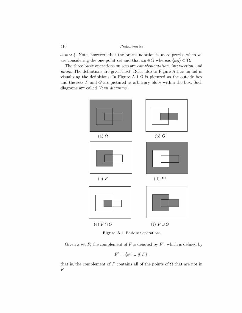
416 Preliminaries

ω = ω0. Note, however, that the braces notation is more precise when we

are considering the one-point set and that ω0 ∈ Ω whereas ω0 ⊂ Ω.

The three basic operations on sets are complementation, intersection, and

union. The definitions are given next. Refer also to Figure A.1 as an aid in

visualizing the definitions. In Figure A.1 Ω is pictured as the outside box

and the sets F and G are pictured as arbitrary blobs within the box. Such

diagrams are called Venn diagrams.

(e) F ∩ G (f) F ∪ G

(c) F (d) F c

(a) Ω (b) G

Figure A.1 Basic set operations

Given a set F, the complement of F is denoted by F c, which is defined by

F c = ω : ω 6∈ F,

that is, the complement of F contains all of the points of Ω that are not in

F.

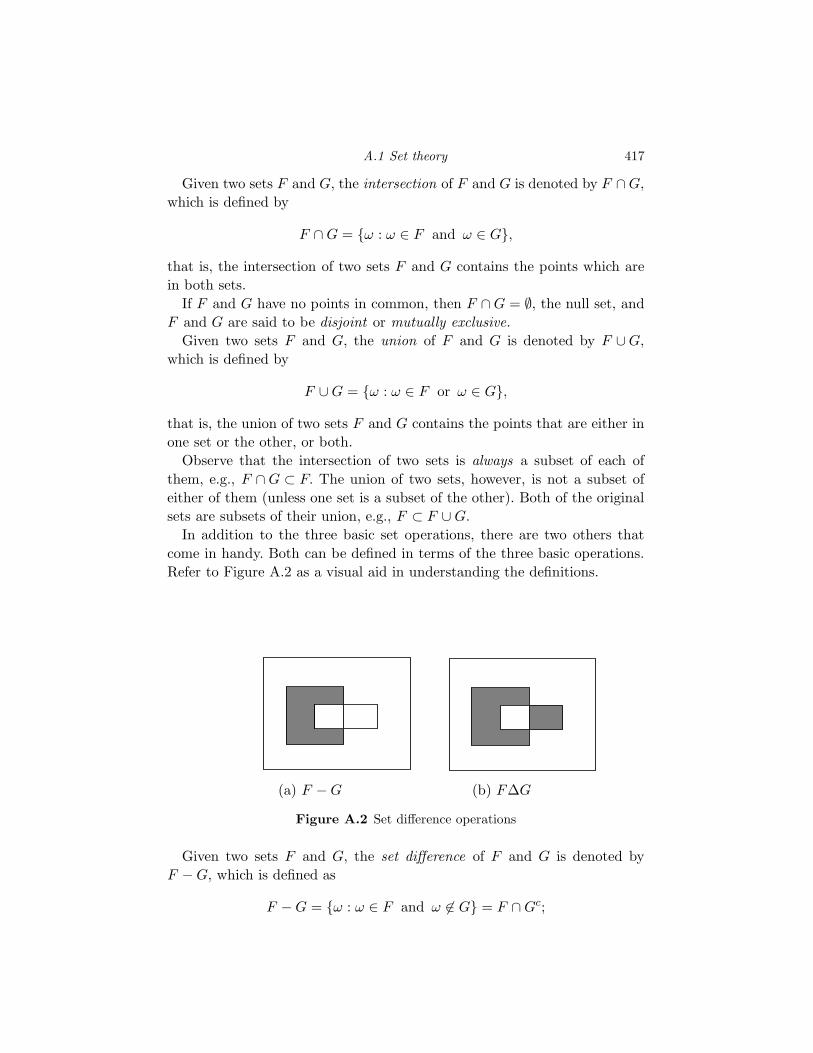
A.1 Set theory 417

Given two sets F and G, the intersection of F and G is denoted by F ∩ G,

which is defined by

F ∩ G = ω : ω ∈ F and ω ∈ G,

that is, the intersection of two sets F and G contains the points which are

in both sets.

If F and G have no points in common, then F ∩ G = ∅, the null set, and

F and G are said to be disjoint or mutually exclusive.

Given two sets F and G, the union of F and G is denoted by F ∪ G,

which is defined by

F ∪ G = ω : ω ∈ F or ω ∈ G,

that is, the union of two sets F and G contains the points that are either in

one set or the other, or both.

Observe that the intersection of two sets is always a subset of each of

them, e.g., F ∩ G ⊂ F. The union of two sets, however, is not a subset of

either of them (unless one set is a subset of the other). Both of the original

sets are subsets of their union, e.g., F ⊂ F ∪ G.

In addition to the three basic set operations, there are two others that

come in handy. Both can be defined in terms of the three basic operations.

Refer to Figure A.2 as a visual aid in understanding the definitions.

(a) F − G (b) F∆G

Figure A.2 Set difference operations

Given two sets F and G, the set difference of F and G is denoted by

F − G, which is defined as

F − G = ω : ω ∈ F and ω 6∈ G = F ∩ Gc;

418 Preliminaries

that is, the difference of F and G contains all of the points in F that are

not also in G. Note that this operation is not completely analogous to the

“minus” of ordinary arithmetic because there is no such thing as a “negative

set.”

Given two sets F and G, their symmetric difference is denoted by F∆G,

which is defined as

F∆G = ω : ω ∈ F or ω ∈ G but not both= (F − G) ∪ (G − F ) = (F ∩ Gc) ∪ (F c ∩ G)

= (F ∪ G) − (F ∩ G);

that is, the symmetric difference between two sets is the set of points that

are in one of the two sets but are not common to both sets. If both sets are

the same, the symmetric difference consists of no points, that is, it is the

empty set. If F ⊂ G, then obviously F∆G = G − F.

Observe that two sets F and G will be equal if and only if F ⊂ G and

G ⊂ F. This observation is often useful as a means of proving that two sets

are identical: first prove that each point in one set is in the other and hence

the first set is subset of the second. Then prove the opposite inclusion.

Surprisingly, this technique is frequently much easier than a direct proof

that two sets are identical by a pointwise argument of commonality.

We will often wish to combine sets in a series of operations and to reduce

the expression for the resulting set to its simplest and most compact form.

Although the most compact form frequently can be seen quickly with the

aid of a Venn diagram, as in Figures A.1 and A.2, to be completely rigorous,

the use of set theory or set algebra to manipulate the basic operations is

required. Table A.1 collects the most important such identities. The first

seven relations can be taken as axioms in an algebra of sets and used to

derive all other relations, including the remaining relations in the table.

Some examples of such derivations follow the table. Readers who are familiar

with Boolean algebra will find a one-to-one analogy between the algebra of

sets and Boolean algebra. DeMorgan’s “laws” (A.6) and (A.10) are useful

when complementing unions of intersections. Relation (A.16) is useful for

writing the union of overlapping sets as a union of disjoint sets. A set and

its complement are always disjoint by relation (A.5).

A.2 Examples of proofs

Relation (A.8). From the definition of intersection and Figure A.1 we verify

the truth of (A.8). Algebraically, we show the same thing from the basic

A.2 Examples of proofs 419

F ∪ G = G ∪ F commutative law (A.1)

F ∪ (G ∪ H) = (F ∪ G) ∪ H associative law (A.2)

F ∩ (G ∪ H) = (F ∩ G) ∪ (F ∩ H)

distributive law (A.3)

(F c)c = F (A.4)

F ∩ F c = ∅ (A.5)

(F ∩ G)c = F c ∪ Gc DeMorgan’s “law” (A.6)

F ∩ Ω = F (A.7)

F ∩ G = G ∩ F commutative law (A.8)

F ∩ (G ∩ H) = (F ∩ G) ∩ H associative law (A.9)

(F ∪ G)c = F c ∩ Gc DeMorgan’s other “law” (A.10)

F ∪ F c = Ω (A.11)

F ∪ ∅ = F (A.12)

F ∪ (F ∩ G) = F = F ∩ (F ∪ G) (A.13)

F ∪ Ω = Ω (A.14)

F ∩ ∅ = ∅ (A.15)

F ∪ G = F ∪ (F c ∩ G) = F ∪ (G − F ) (A.16)

F ∪ (G ∩ H) = (F ∪ G) ∩ (F ∪ H) distributive law (A.17)

Ωc = ∅ (A.18)

F ∪ F = F (A.19)

F ∩ F = F (A.20)

Table A.1 Set algebra

seven axioms: From (A.4) and (A.6) we have that

A ∩ B = ((A ∩ B)c)c = (Ac ∪ Bc)c,

and using (A.1), (A.4), and (A.6), this becomes

(Bc ∪ Ac)c = (Bc)c ∩ (Ac)c

as desired.

Relation (A.18). Set F = Ω in (A.5) to obtain Ω ∩ Ωc = ∅, which with (A.7)

420 Preliminaries

and (A.8) yields (A.18).

Relation (A.11). Complement (A.5), (F c ∩ F )c = ∅c, and hence, using

(A.6), (F c ∪ F ) = ∅c, and finally, using (A.4) and (A.18), F c ∪ F = Ω.

Relation (A.12). Using F c in (A.7): F c ∩ Ω = F c. Complementing the result:

(F c ∩ Ω)c = (F c)c = F (by (A.4)). Using (A.6): (F c ∩ Ω)c = F ∪ Ωc = F.

From (A.18) Ωc = ∅, yielding (A.12).

Relation (A.20). Set G = F and H = F c in (A.3) to obtain

F ∩ (F ∪ F c) = (F ∩ F ) ∪ (F ∩ F c) = F ∩ F using (A.5) and (A.12).

Applying (A.11) and (A.7) to the left-hand side of this relation yields

F ∩ Ω = F = F ∩ F.

Relation (A.19). Complement (A.20) using (A.6) and replace F c by F .

The proofs for the examples were algebraic in nature, manipulating the

operations based on the axioms. Proofs can also be constructed based on

the definitions of the basic operations. For example, DeMorgan’s law can

be proved directly by considering individual points. To prove that (F ∩G)c = F c ∪ Gc it suffices to show separately that (F ∩ G)c ⊂ F c ∪ Gc and

F c ∪ Gc ⊂ (F ∩ G)c. Suppose that ω ∈ (F ∩ G)c, then ω 6∈ F ∩ G from the

definition of complement and hence ω 6∈ F or ω 6∈ G from the definition of

intersection (if ω were in both, it would be in the intersection). Thus either

ω ∈ F c or ω ∈ Gc and hence ω ∈ F c ∪ Gc. Conversely, if ω ∈ F c ∪ Gc, then

ω ∈ F c or ω ∈ Gc, and hence either ω 6= F or ω 6= G, which implies that

ω 6= F ∩ G, which in turn implies that ω ∈ (F ∩ G)c, completing the proof.

We will have occasion to deal with more general unions and intersections,

that is, unions or intersections of more than two or three sets. As long as the

number of unions and intersections is finite, the generalizations are obvious.

The various set theoretic relations extend to unions and intersections of

finite collections of sets. For example, DeMorgan’s law for finite collections

of sets is

(n⋂

i=1

Fi

)c

=n⋃

i=1

F ci . (A.21)

This result can be proved using the axioms or by induction. Point arguments

are often more direct. Define the set on the left-hand side of the equation

as G and that on the right-hand side as H and prove G = H by considering

A.2 Examples of proofs 421

individual points. This is done by separately showing that G ⊂ H and H ⊂G, which implies the two sets are the same. To show that G ⊂ H, let ω ∈G = (

⋂ni=1 Fi)

c, which means that ω 6∈ ⋂ni=1 Fi, which means that ω 6∈ Fi for

some i or, equivalently, that ω ∈ F ci for some i. This means that ω ∈ ⋃n

i=1 F ci

and hence that ω ∈ H. Thus G ⊂ H since we have shown that every point

in G is also in H. The converse containment follows in a similar manner. If

ω ∈ H =⋃n

i=1 F ci , the ω ∈ F c

i for some i and hence ω 6∈ Fi for some i. This

implies that ω 6∈ ⋂ni=1 Fi and hence that ω ∈ G, completing the proof.

The operations can also be defined for quite general infinite collections

of sets as well. Say that we have an indexed collection of sets Ai; i ∈ I,sometimes denoted Aii∈I , for some index set I. In other words, this col-

lection is a set whose elements are sets — one set Ai for each possible value

of an index i drawn from I. We call such a collection a family or class of

sets. (To avoid confusion we never say a “set of sets.”) The index set Ican be thought of as numbering the sets. Typical index sets are the set Z+

of all nonnegative integers, Z = . . . ,−1, 0, 1, . . ., or the real line ℜ. The

index set may be finite in that it has only a finite number of entries, say

I = Zk = 0, 1, . . . , k − 1. The index set is said to be countably infinite if

its elements can be counted, that is, can be put into a one-to-one correspon-

dence with a subset of the nonnegative integers Z+; e.g., Z+ or Z itself. If

an index set has an infinity of elements, but the elements cannot be counted,

then it is said to be uncountably infinite, for example ℜ or the unit interval

[0, 1] (see Problem a.11).

The family of sets is said to be finite, countable, or uncountable if the

respective index set is finite, countable, or uncountable. As an example,

the family of sets [0, 1/r); r ∈ I is countable if I = Z and uncountable if

I = ℜ. Another way of describing countably infinite sets is that they can be

put into one-to-one correspondence with the integers. For example, the set

of rational numbers is countable because it can be enumerated, the set of

irrational numbers is not.

The obvious extensions of the pairwise definitions of union and intersec-

tion will now be given. Given an indexed family of sets Ai; i ∈ I, define

the union by

⋃

i∈IAi = ω : ω ∈ Ai for at least one i ∈ I

and define the intersection by

⋂

i∈IAi = ω : ω ∈ Ai for all i ∈ I.

422 Preliminaries

In certain special cases we make the notation more specific for particular

index sets. For example, if I = 0, . . . , n − 1, then we write the union and

intersection as

n−1⋃

i=0

Ai and

n−1⋂

i=0

Ai

respectively.

A collection of sets Fi; i ∈ I is said to be disjoint or pairwise disjoint

or mutually exclusive if

Fi ∩ Fj = ∅; all i, j ∈ I, i 6= j,

that is, if no sets in the collection contain points contained by other sets in

the collection.

The class of sets is said to be collectively exhaustive or to exhaust the

space if

⋃

i∈IFi = Ω,

that is, together the Fi contain all the points of the space.

A collection of sets Fj ; i ∈ I is called a partition of the space Ω if the

collection is both disjoint and collectively exhaustive. A collection of sets

Fi; i ∈ I is said to partition a set G if the collection is disjoint and the

union of all of its members is identical to G.

A.3 Mappings and functions

We make much use of mappings of functions from one space to another. This

is of importance in a number of applications. For example, the waveforms

and sequences that we considered as members of an abstract space describ-

ing the outputs of a random process are just functions of time – for each

value of time t in some continuous or discrete collection of possible times we

assigned some output value to the function. As a more complicated example,

consider a binary digit that is transmitted to a receiver at some destination

by sending either plus or minus V volts through a noisy environment called

a “channel.” At the receiver a decision is made whether +V or −V was sent.

The receiver puts out a 1 or a 0, depending on the decision. In this example

three mappings are involved: the transmitter maps a binary symbol in 0, 1into either +V or −V. During transmission, the channel has an input either

A.4 Linear algebra 423

+V or −V and produces a real number, not usually equal to 0, 1, +V, or

−V. At the receiver, a real number is viewed and a binary number produced.

We will encounter a variety of functions or mappings, from simple arith-

metic operations to general filtering operations. We now introduce some

common terminology and notation for handling such functions. Given two

abstract spaces Ω and A, an A-valued function or mapping F or, in more

detail, f : Ω → A, is an assignment of a unique point in A to each point in

Ω; that is, given any point ω ∈ Ω, f(ω) is some value in A. Ω is called the

domain or domain of definition of the function f , and A is called the range

of f . Given any sets F ⊂ Ω and G ⊂ A, define the image of F (under f) as

the set

f(F ) = a : a = f(ω) for some ω ∈ F

and the inverse image (also called the preimage) of G (under f) as the set

f−1(G) = ω : f(ω) ∈ G.

Thus f(F ) is the set of all points in A obtained by mapping points in F,

and f−1(G) is the set of all points in Ω that map into G.

For example, let Ω = [−1, 1] and A = [−10, 10]. Given the function f(ω) =

ω2 with domain Ω and range A, define the sets F = (−1/2, 1/2) ⊂ Ω and

G = (−1/4, 1) ⊂ A. Then f(F ) = [0, 1/4) and f−1(G) = [−1, 1]. As you can

see from this example, not all points in G have to correspond to points in F .

In fact, the inverse image can be empty; e.g., continuing the same example,

f−1((−1/4, 0)) = ∅.The image of the entire space Ω is called the range space of f , and it

need not equal the range; the function f could map the whole input space

into a single point in A. For example, f : ℜ → ℜ defined by f(r) = 1, all

r, has a range space of a single point. If the range space equals the range,

the mapping is said to be onto. (Is the mapping f of the preceding example

onto? What is the range space? Is the range unique?)

A mapping f is called one-to-one if x 6= y implies that f(x) 6= f(y).

A real valued function f is said to be continuous at r0 if given any ǫ > 0

there is a δ > 0 such that if |r − r0| ≤ δ, then |f(r) − f(r0)| ≤ ǫ.

A.4 Linear algebra

We collect a few definitions and results for vectors, matrices, and determi-

nants.

There is a variety of notational styles for vectors. Historically a com-

424 Preliminaries

mon form was to use boldface, as in x = (x0, x0, . . . , xk−1), to denote a k-

dimensional vector with k components xi, i = 0, 1, . . . , k − 1. When dealing

with linear algebra, however, it is most commonly the convention to assume

that vectors are column vectors, e.g.,

x =

x0

x1...

xk−1

,

or, as an in-line equation, x = (x0, x0, . . . , xk−1)t, where t denotes “trans-

pose.” We will often be lazy and write vectors inline without explicitly de-

noting the transpose unless it is needed, e.g., in vector/matrix equations.

Although boldface makes it clear which symbols are vectors and which are

scalars, in modern practice it is more common to drop the distinction and

not use boldface, i.e., to write a vector as simply x = (x0, x1, . . . , xk−1) or,

if it is desired to make clear it is a column vector, as x = (x0, x1, . . . , xk−1)t.

Both boldface and nonboldface notations are used in this book. Generally,

early on the boldface notation is used to clarify when vectors or scalars are

being used while later in the book boldface is often dropped.

The inner product (or dot product) of two real-valued n-dimensional vec-

tors y and n is defined by the scalar value

xty =

n−1∑

i=0

xiyi. (A.22)

If the vectors are more generally complex-valued, then the transpose is re-

placed by a conjugate transpose

x∗y =

n−1∑

i=0

x∗i yi. (A.23)

A matrix is a rectangular array of numbers

A =

a0,0 a0,1 a0,2 · · · a0,n−1

a1,0 a1,1 a1,2 · · · a1,n−1

· · · · ·· · · · ·· · · · ·am−1,0 am−1,1 am−1,2 · · · am−1,n−1

with m rows and n columns. Boldface notation is also used for matrices. If

m = n the matrix is said to be square. A matrix is symmetric if At = A,

A.4 Linear algebra 425

where At is the transpose of the matrix A, that is, the n × m matrix whose

k, jth element is (At)k,j = aj,k. If the matrix has complex elements and A∗ =

A, where ∗ denotes conjugate transpose so that (A∗)k,j = a∗j,k, then A is said

to be Hermitian.

The product of an m × n matrix and an n-dimensional vector y = Ax is

an m dimensional vector with components

yi =

n−1∑

k=0

ai,kxk,

that is, the inner product of x and the ith row of A.

The outer product of two n-dimensional vectors y and n is defined as the

n × n matrix

xyt =

x0y0 x0y1 x0y2 · · · x0yn−1

x1y0 x1y1 x1y2 · · · x1yn−1

· · · · ·· · · · ·· · · · ·xn−1y0 xn−1y1 xn−1y2 · · · xn−1yn−1

(A.24)

Given a square matrix A, a scalar λ is called an eigenvalue and a vector

u is called an eigenvector if

Au = λu. (A.25)

An n × n matrix has n eigenvalues and eigenvectors, but they need not

be distinct. Eigenvalues provide interesting formulas for two attributes of

matrices, the trace defined by

Tr(A) =

n−1∑

i=0

ai,i

and the determinant of the matrix det(A):

Tr(A) =n−1∑

i=0

λi (A.26)

det(A) =n−1∏

i=0

λi (A.27)

The arithmetic–geometric means inequality says that the arithmetic mean

of a collection of real positive numbers λi is bounded below by the geometric

426 Preliminaries

mean:

1

n

n−1∑

i=0

λi ≥(

n−1∏

i=0

λi

) 1n

(A.28)

with equality if and only if the λ are all the same. Application of the in-

equality to the eigenvalue representation of the determinant and trace in the

case where the eigenvalues are real and positive (e.g., an Hermitian matrix)

provides the inequality

1

nTr(A) ≥ (det(A))1/n (A.29)

with equality if and only if the eigenvalues are all constant.

A similar argument provides an inequality for the harmonic mean, the

arithmetic mean of the reciprocals. If the matrix A has real and positive

eigenvalues, then

1

nTr(A) ≥ (det(A))1/n ≥ n

Tr(A−1). (A.30)

A square Hermitian matrix A can be diagonalized into the form

A = UΛU∗, (A.31)

where Λ is the diagonal matrix with diagonal entries Λ(k, k) = λk, the kth

eigenvalue of the matrix, and where U is a unitary matrix, that is, U∗ = U−1.

The inner product and outer product of two vectors can be related as

xty = Tr(xyt). (A.32)

Given an n-dimensional vector x and an n × n matrix A, the product

xtAx =

n−1∑

k=0

n−1∑

j=0

xkxjak,j

is called a quadratic form. If the matrix A is such that xtAx ≥ 0, the matrix is

said to be nonnegative definite. If the matrix is such that xtAx > 0, then the

matrix is said to be positive definite. These are the definitions for real-valued

vectors and matrices. For complex vectors and matrices use the conjugate

transpose instead of the transpose. If a matrix is positive definite, then its

eigenvalues are all strictly positive and hence so is its determinant.

A quadratic form can also be written as

xtAx = Tr(Axxt). (A.33)

A.5 Linear system fundamentals 427

If a matrix A is positive definite and Hermitian (e.g., real and symmet-

ric), then its square root A1/2 is well-defined as UΛ1/2U∗. In particular,

A1/2A1/2 = A and (A1/2)−1 = (A−1)1/2.

A.5 Linear system fundamentals

In general, a system L is a mapping of an input time function or input signal ,

x = x(t); t ∈ T into an output time function or output signal, L(x) = y =

y(t); t ∈ T . We now use T to denote the index set or domain of definition

instead of I to emphasize that the members of the set correspond to “time.”

Usually the functions take on real or complex values of each value of time

t in T . The system is called a discrete time system if T is discrete, e.g., Zor Z+, and it is called a continuous time system if T is continuous, e.g.,

ℜ or [0,∞). If only nonnegative times are allowed, e.g., T is Z+ or [0,∞),

the system is called a one-sided or single-sided system. If time can go on

infinitely in both directions, then it is said to be a two-sided system.

A system L is said to be linear if the mapping is linear, that is, for all

complex (or real) constants a and b and all input functions x1 and x2

L(ax1 + bx2) = aL(x1) + bL(x2). (A.34)

There are many ways to define or describe a particular linear system: one

can provide a constructive rule for determining the output from the input;

e.g., the output may be a weighted sum or integral of values of the input.

Alternatively, one may provide a set of equations whose solution determines

the output from the input, e.g., differential or difference equations involv-

ing the input and output at various times. Our emphasis is on the former

constructive technique, but we shall occasionally consider examples of other

techniques.

The most common and the most useful class of linear systems comprises

systems that can be represented by a convolution, that is, where the output

is described by a weighted integral or sum of input values. We first consider

continuous time systems and then turn to discrete time systems.

For t ∈ T ⊂ ℜ, let x(t) be a continuous time input to a system with output

y(t) defined by the superposition integral

y(t) =

∫

s:t−s∈Tx(t − s)ht(s) ds. (A.35)

The function ht(t) is called the impulse response of the system since it can

be considered the output of the system at time t which results from an input

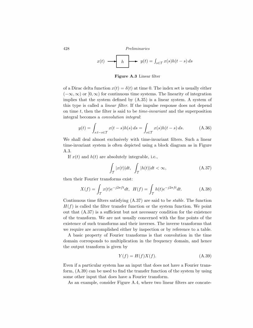
428 Preliminaries

x(t) - h - y(t) =∫s∈T x(s)h(t − s) ds

Figure A.3 Linear filter

of a Dirac delta function x(t) = δ(t) at time 0. The index set is usually either

(−∞,∞) or [0,∞) for continuous time systems. The linearity of integration

implies that the system defined by (A.35) is a linear system. A system of

this type is called a linear filter. If the impulse response does not depend

on time t, then the filter is said to be time-invariant and the superposition

integral becomes a convolution integral:

y(t) =

∫

s:t−s∈Tx(t − s)h(s) ds =

∫

s∈Tx(s)h(t − s) ds. (A.36)

We shall deal almost exclusively with time-invariant filters. Such a linear

time-invariant system is often depicted using a block diagram as in Figure

A.3.

If x(t) and h(t) are absolutely integrable, i.e.,∫

T|x(t)|dt,

∫

T|h(t)|dt < ∞, (A.37)

then their Fourier transforms exist:

X(f) =

∫

Tx(t)e−j2πftdt, H(f) =

∫

Th(t)e−j2πftdt. (A.38)

Continuous time filters satisfying (A.37) are said to be stable. The function

H(f) is called the filter transfer function or the system function. We point

out that (A.37) is a sufficient but not necessary condition for the existence

of the transform. We are not usually concerned with the fine points of the

existence of such transforms and their inverses. The inverse transforms that

we require are accomplished either by inspection or by reference to a table.

A basic property of Fourier transforms is that convolution in the time

domain corresponds to multiplication in the frequency domain, and hence

the output transform is given by

Y (f) = H(f)X(f). (A.39)

Even if a particular system has an input that does not have a Fourier trans-

form, (A.39) can be used to find the transfer function of the system by using

some other input that does have a Fourier transform.

As an example, consider Figure A.4, where two linear filters are concate-

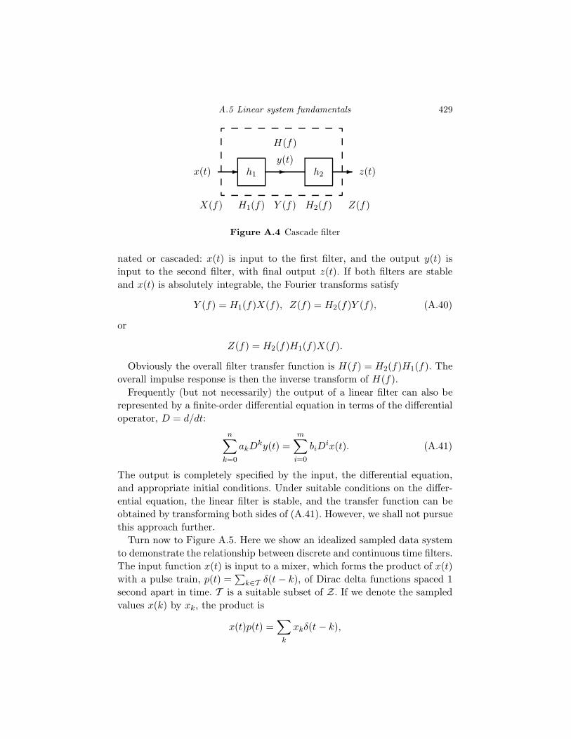
A.5 Linear system fundamentals 429

x(t) - h1-y(t)

h2- z(t)

H(f)

X(f) H1(f) Y (f) H2(f) Z(f)

Figure A.4 Cascade filter

nated or cascaded: x(t) is input to the first filter, and the output y(t) is

input to the second filter, with final output z(t). If both filters are stable

and x(t) is absolutely integrable, the Fourier transforms satisfy

Y (f) = H1(f)X(f), Z(f) = H2(f)Y (f), (A.40)

or

Z(f) = H2(f)H1(f)X(f).

Obviously the overall filter transfer function is H(f) = H2(f)H1(f). The

overall impulse response is then the inverse transform of H(f).

Frequently (but not necessarily) the output of a linear filter can also be

represented by a finite-order differential equation in terms of the differential

operator, D = d/dt:

n∑

k=0

akDky(t) =

m∑

i=0

biDix(t). (A.41)

The output is completely specified by the input, the differential equation,

and appropriate initial conditions. Under suitable conditions on the differ-

ential equation, the linear filter is stable, and the transfer function can be

obtained by transforming both sides of (A.41). However, we shall not pursue

this approach further.

Turn now to Figure A.5. Here we show an idealized sampled data system

to demonstrate the relationship between discrete and continuous time filters.

The input function x(t) is input to a mixer, which forms the product of x(t)

with a pulse train, p(t) =∑

k∈T δ(t − k), of Dirac delta functions spaced 1

second apart in time. T is a suitable subset of Z. If we denote the sampled

values x(k) by xk, the product is

x(t)p(t) =∑

k

xkδ(t − k),

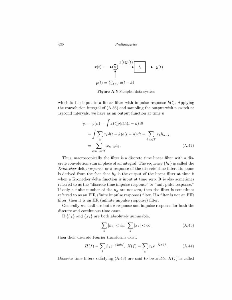
430 Preliminaries

x(t) - m× -x(t)p(t)

h - y(t)

6

p(t) =∑

k∈T δ(t − k)

Figure A.5 Sampled data system

which is the input to a linear filter with impulse response h(t). Applying

the convolution integral of (A.36) and sampling the output with a switch at

1second intervals, we have as an output function at time n

yn = y(n) =

∫x(t)p(t)h(t − n) dt

=

∫ ∑

k

xkδ(t − k)h(t − n) dt =∑

k:k∈Txkhn−k

=∑

k:n−k∈Txn−khk. (A.42)

Thus, macroscopically the filter is a discrete time linear filter with a dis-

crete convolution sum in place of an integral. The sequence hk is called the

Kronecker delta response or δ-response of the discrete time filter. Its name

is derived from the fact that hk is the output of the linear filter at time k

when a Kronecker delta function is input at time zero. It is also sometimes

referred to as the “discrete time impulse response” or “unit pulse response.”

If only a finite number of the hk are nonzero, then the filter is sometimes

referred to as an FIR (finite impulse response) filter. If a filter is not an FIR

filter, then it is an IIR (infinite impulse response) filter.

Generally we shall use both δ-response and impulse response for both the

discrete and continuous time cases.

If hk and xk are both absolutely summable,

∑

k

|hk| < ∞,∑

k

|xk| < ∞, (A.43)

then their discrete Fourier transforms exist:

H(f) =∑

k

hke−j2πkf , X(f) =

∑

k

xke−j2πkf . (A.44)

Discrete time filters satisfying (A.43) are said to be stable. H(f) is called

A.6 Problems 431

the filter transfer function. The output transform is given by

Y (f) = H(f)X(f). (A.45)

The example of Figure A.4 applies for discrete time as well as continuous

time.

For convenience and brevity, we shall occasionally use a general notation

F to denote both the discrete and continuous Fourier transforms; that is,

F(x) =

∫

Tx(t)e−j2πft dt T continuous

∑

k∈Txke

−j2πfk T discrete

. (A.46)

A more general discrete time linear system is described by a difference

equation of the form∑

k

akyn−k =∑

i

bixn−k. (A.47)

Observe that the convolution of (A.42) is a special case of the above where

only one of the ak is not zero. Observe also that the difference equation

(A.47) is a discrete time analog of the differential equation (A.41). As in that

case, to describe an output completely one has to specify initial conditions.

A continuous time or discrete time filter is said to be causal if the pulse

response or impulse response is zero for negative time; that is, if a discrete

time pulse response hk satisfies hk = 0 for k < 0 or a continuous time impulse

response h(t) satisfies h(t) = 0 for t < 0.

A.6 Problems

1. Use the first seven relations to prove relations (A.10), (A.13), and (A.16).

2. Use relation (A.16) to obtain a partition Gi; i = 1, 2, . . . , k of Ω from an ar-

bitrary finite class of collectively exhaustive sets Fi; i = 1, 2, . . . , k with the

property that Gi ⊂ Fi for all i and

i⋃

j=1

Gj =

i⋃

j=1

Fj all i.

Repeat for a countable collection of sets Fi. (You must prove that the given

collection of sets is indeed a partition.)

3. If Fi partitions Ω, show that G ∩ Fi partitions G.

4. Show that F ⊂ G implies that F ∩ G = F, F ∪ G = G, and Gc ⊂ F c.

432 Preliminaries

5. Show that if F and G are disjoint, then F ⊂ Gc.

6. Show that F ∩ G = (F ∪ G) − (F∆G).

7. Let Fr = [0, 1/r), r ∈ (0, 1]. Find⋃

r∈(0,1]Fr and⋂

r∈(0,1]Fr.

8. Prove the countably infinite version of DeMorgan’s “laws.” For example, given

a sequence of sets Fi; i = 1, 2, . . . , then

∞⋂

i=1

Fi =

( ∞⋃

i=1

F ci

)c

.

9. Define the subsets of the real line

Fn =

r : |r| >

1

n

,

and

F = 0.

Show that

F c =∞⋃

n=1

Fn.

10. Let Fi, i = 1, 2, . . . be a countable sequence of “nested” closed intervals whose

length is not zero, but tends to zero; i.e., for every i, Fi = [ai, bi] ⊂ Fi−1 ⊂Fi−2 . . . and bi − ai → 0 and i → ∞. What are the points in

⋂∞i=1Fi?

11. Prove that the interval [0, 1] cannot be put into one-to-one correspondence with

the set of integers as follows: suppose that there is such a correspondence so that

x1, x2, x3, . . . is a listing of all numbers in [0, 1]. Use Problem A.10 to construct

a set that consists of a point not in this listing. This contradiction proves the

statement.

12. Show that inverse images preserve set theoretic operations, that is, given f : Ω →A and sets F and G in A, then

f−1(F c) = (f−1(F ))c.

f−1(F ∪ G) = f−1(F ) ∪ f−1(G),

and

f−1(F ∩ G) = f−1(F ) ∩ f−1(G).

If Fi, i ∈ I is an indexed family of subsets of A that partitions A, show that

f−1(Fi); i ∈ I is a partition of Ω. Do images preserve set theoretic operations

in general? (Prove that they do or provide a counterexample.)

13. An experiment consists of rolling two four-sided dice (each having faces labeled

1, 2, 3, 4) on a glass table. Depict the space Ω of possible outcomes. Define two

functions on Ω: X1(ω) = the sum of the two down faces and X2(ω) = the product

A.6 Problems 433

of the two down faces. Let A1 denote the range space of X1, A2 the range space of

X2, and A12 the range space of the vector-valued function X = (X1, X2), that is,

X (ω) = (X1(ω), X2(ω)). Draw in both Ω and A12 the set ω : X1(ω) < X2(ω).The cartesian product

∏2i=1Ai of two sets is defined as the collection of all pairs

of elements, one from each set, that is

2∏

i=1

Ai = all a, b : a ∈ A1, b ∈ A2.

Is it true above that A12 =∏2

i=1Ai?

14. Let Ω = [0, 1] and A be the set of all infinite binary vectors. Find a one-to-one

mapping from Ω to A, being careful to note that some rational numbers have

two infinite binary representations (e.g., 1/2 = 0.1000 . . . = 0.0111 . . . in binary).

15. Can you find a one-to-one mapping from:

(a) [0, 1] to [0, 2)?

(b) [0, 1] to the unit square [0, 1]2?

(c) Z to Z+? When is it possible to find a one-to-one mapping from one space

to another?

16. Suppose that a voltage is measured that takes values in Ω = [0, 15]. The voltage

is mapped into the finite space A = 0, 1, . . . , 15 for transmission over a digital

channel. A mapping of this type is called a quantizer. What is the best mapping

in the sense that the maximum error is minimized?

17. Let A be as in Problem A.16, i.e., the space of 16 messages which is mapped into

the space of 16 waveforms, B = cosnt, n = 0, 1, . . . , 15; t ∈ [0, 2π]. The selected

waveform from B is transmitted on a waveform channel, which adds noise; i.e., B

is mapped into C = set of all possible waveforms y(t) = cosnt + noise(t); t ∈[0, 2π]. (This is a random mapping in a sense that is explained in the text.)

Find a good mapping from C into D = A. The set D is the decision space and

the mapping is called a decision rule. (In other words, how would you perform

this mapping knowing little of probability theory? Your mapping should at least

give the correct decision if the noise is absent or small.)

18. A continuous time linear filter has impulse response h(t) given by e−at for t ≥ 0

and 0 for t < 0, where a is a positive constant. Find the transfer function H(f)

of the filter. Is the filter stable? What happens if a = 0?

19. A discrete time linear filter has δ-response hk given by rk for k ≥ 0 and 0 for

k < 0, where r has magnitude strictly less than 1, find the transfer function H(f).

(Hint: use the geometric series formula.) Is the filter stable? What happens if

r = 1? Assume that |r| < 1. Suppose that the input xk = 1 for all nonnegative k

and xk = 0 for all negative k is put into the filter. Find a simple expression for

the output as a function of time. Does the transform of the output exist?

20. A continuous time system is described by the following relation: an input x =

434 Preliminaries

x(t); t ∈ ℜ is defined for each t by

y(t) = (a0 + a1x(t)) cos(2πf0t + θ),

where a0, a1, f0, and θ are fixed parameters. (This system is called an amplitude

modulation (AM) system.) Under what conditions on the parameters is this

system linear? Is it time-invariant?

21. Suppose that x = x(t); t ∈ R, where R = (−∞,∞) is the real line, is a con-

tinuous time signal defined by

x(t) =

1 |t| ≤ T

0 otherwise,

where T > 0 is a fixed parameter. This signal is put into a linear, time-invariant

(LTI) filter described by an impulse response h = h(t); t ∈ R, where

h(t) =

e−t t ≥ 0

0 otherwise.

(a) Find the Fourier transform X of x, i.e.,

X(f) =

∫ ∞

−∞x(t)e−j2πft dt; f ∈ R,

where j =√−1. Find the Fourier transform H of h.

(b) Find y, the output signal of the LTI filter, and its Fourier transform Y .

22. Suppose that x = xn; n ∈ Z, where Z is the set of all integers

. . . ,−2,−1, 0, 1, 2, . . ., is a discrete time signal defined by

xn =

rn n ≥ 0

0 otherwise,

where r is a fixed parameter satisfying |r| < 1, is put into a linear, time-invariant

(LTI) filter described by a Kronecker delta response h = hn; n ∈ Z, where

hn =

1 n = 0, 1, . . . , N − 1

0 otherwise,

where N > 0 is a fixed integer. This filter is sometimes called a “comb filter.”

Note that the Kronecker delta response is the response to the filter when the

input is δn, the Kronecker delta defined as

δn =

1 n = 0

0 otherwise.

A.6 Problems 435

(a) Find the (discrete time) Fourier transform X of x, i.e.,

X(f) =

∞∑

n=−∞xne−j2πfn ; f ∈ (−1/2, 1/2).

Find the Fourier transform H of h.

(b) Find y, the output signal of the LTI filter, and its Fourier transform Y .

23. Evaluate the following integrals:

(a)∫ ∫

x,y:0≤x,y≤2;√

(x−2)2+(y−2)2≤1

dx dy

(b)∫ ∞

0

dxe−x

∫ x

0

dye−y.

24. Evaluate the following integrals:

(a)∫ ∫

x,y:|x|+|y|≤r

dx dy

(b)∫ ∞

0

dx

∫ ∞

x

dye−y

(c)∫ ∫

x,y:0≤x2≤y≤1

dx dy.

Appendix B

Sums and integrals

In this appendix a few useful definitions and results are gathered for refer-

ence.

B.1 Summation

The sum of consecutive integers

n∑

k=1

k =n(n + 1)

2. (B.1)

Proof The result is easily proved by induction, which requires demonstrating

the truth of the formula for n = 1 (which is obvious) and showing that if the

formula is true for any positive integer n, then it must also be true for n + 1.

This follows since if Sn =∑n

k=1 k and we assume that Sn = n(n + 1)/2, then

necessarily

Sn+1 = Sn + (n + 1)

= (n + 1)(n

2+ 1)

=(n + 1)(n + 2)

2,

proving the claim. 2

436

B.1 Summation 437

The sum of consecutive squares of integers

n∑

k=1

k2 =1

3n3 +

1

2n2 +

1

6n. (B.2)

The sum can also be expressed as

n∑

k=1

k2 =(2n + 1)(n + 1)n

6.

Proof This can also be proved by induction, but for practice we note another

approach. Just as in solving differential or difference equations, one can

guess a general form of solution and solve for unknowns. Since summing k

up to n had a second-order solution in n, one might suspect that solving

for a sum up to n of squares of k would have a third-order solution in

n, that is, a solution of the form f(n) = an3 + bn2 + cn + d for some real

numbers a, b, c, d. Assume for the moment that this is the case, then if f(n) =∑nk=1 k2, clearly n2 = f(n) − f(n − 1) and hence with a little algebra

n2 = an3 + bn2 + cn + d − a(n − 1)3 + b(n − 1)2 + c(n − 1) + d

= 3an2 + (2b − 3a)n + (a − b + c).

This can only be true for all n however if 3a = 1 so that a = 1/3, if 2b − 3a =

0 so that b = 3a/2 = 1/2, and if a − b + c = 0 so that c = b − a = 1/6. This

leaves d, but the initial condition that f(1) = 1 implies d = 0. 2

The geometric progression

Given a complex constant a,

n−1∑

k=0

ak =1 − an

1 − a, (B.3)

and if |a| < 1 this sum is convergent and

∞∑

k=0

ak =1

1 − a. (B.4)

438 Sums and integrals

Proof There are, in fact, many ways to prove this result. Perhaps the sim-

plest is to define the sum with n terms Sn =∑n−1

k=0 ak and observe that

(1 − a)Sn =

n−1∑

k=0

ak − a

n−1∑

k=0

ak

=

n−1∑

k=0

ak −n∑

k=1

ak

= 1 − an,

proving (B.3). Other methods of proof include induction and solving the

difference equation Sn = Sn−1 + an−1. Proving the finite n result gives the

infinite sum since if |a| < 1,

∞∑

k=0

ak = limn→∞

Sn =1

1 − a. (B.5)

For the reader who might be rusty with limiting arguments, this follows

since

|Sn − 1

1 − a| = | an

1 − a| =

|a|n|1 − a| → 0

as n → ∞ since by assumption |a| < 1. 2

First moment of the geometric progression

Given q ∈ (0, 1),

∞∑

k=0

kqk−1 =1

(1 − q)2. (B.6)

Proof Since kqk−1 =d

dqqk and interchanging differentiation and summa-

tion,

∞∑

k=0

kqk−1 =d

dq

∞∑

k=0

qk =d

dq(1 − q)−1,

where we have used the geometric series sum formula. 2

Second moment of the geometric progression

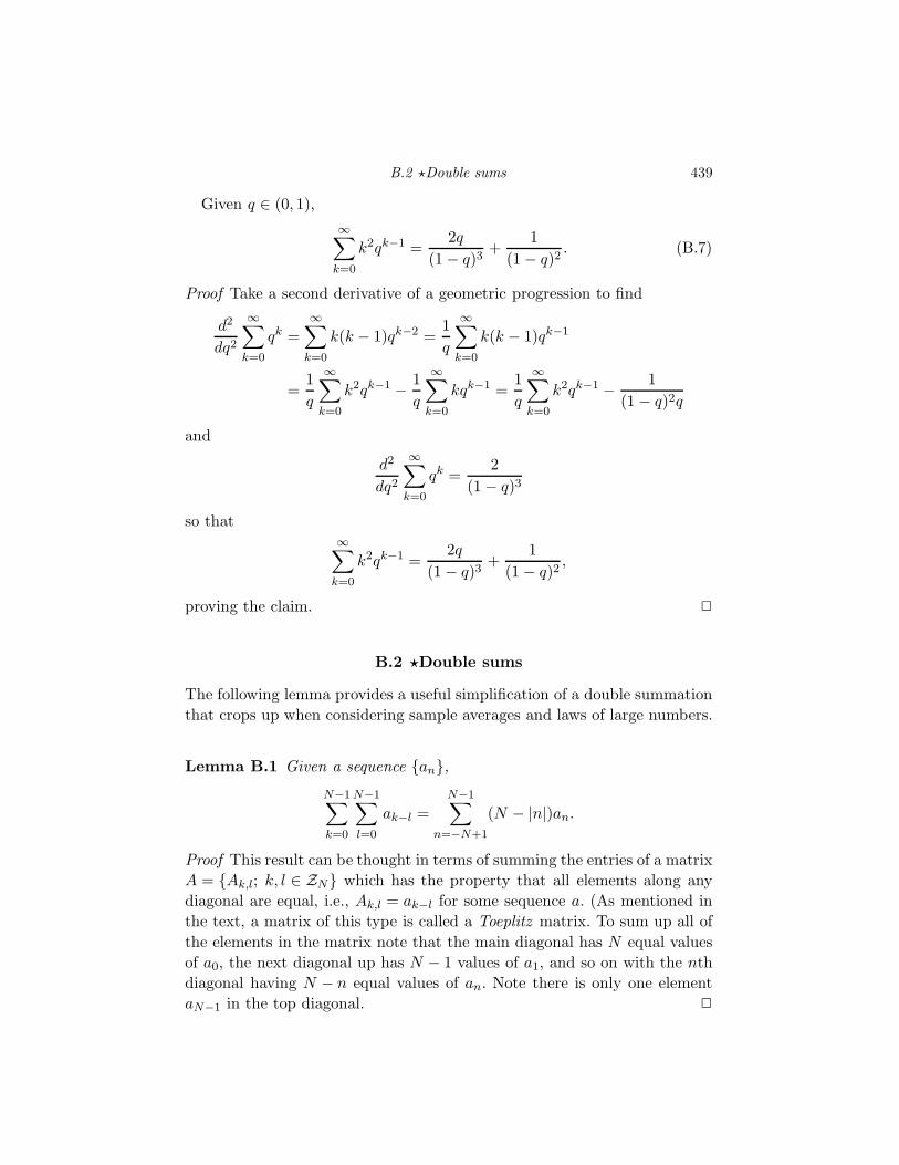
B.2 ⋆Double sums 439

Given q ∈ (0, 1),

∞∑

k=0

k2qk−1 =2q

(1 − q)3+

1

(1 − q)2. (B.7)

Proof Take a second derivative of a geometric progression to find

d2

dq2

∞∑

k=0

qk =

∞∑

k=0

k(k − 1)qk−2 =1

q

∞∑

k=0

k(k − 1)qk−1

=1

q

∞∑

k=0

k2qk−1 − 1

q

∞∑

k=0

kqk−1 =1

q

∞∑

k=0

k2qk−1 − 1

(1 − q)2q

and

d2

dq2

∞∑

k=0

qk =2

(1 − q)3

so that∞∑

k=0

k2qk−1 =2q

(1 − q)3+

1

(1 − q)2,

proving the claim. 2

B.2 ⋆Double sums

The following lemma provides a useful simplification of a double summation

that crops up when considering sample averages and laws of large numbers.

Lemma B.1 Given a sequence an,N−1∑

k=0

N−1∑

l=0

ak−l =

N−1∑

n=−N+1

(N − |n|)an.

Proof This result can be thought in terms of summing the entries of a matrix

A = Ak,l; k, l ∈ ZN which has the property that all elements along any

diagonal are equal, i.e., Ak,l = ak−l for some sequence a. (As mentioned in

the text, a matrix of this type is called a Toeplitz matrix. To sum up all of

the elements in the matrix note that the main diagonal has N equal values

of a0, the next diagonal up has N − 1 values of a1, and so on with the nth

diagonal having N − n equal values of an. Note there is only one element

aN−1 in the top diagonal. 2

440 Sums and integrals

The next result is a limiting result for sums of the type considered in the

previous lemma.

Lemma B.2 Suppose that an; n ∈ Z is an absolutely summable sequence,

i.e., that

∞∑

n=−∞|an| < ∞.

Then

limN→∞

N−1∑

n=−N+1

(1 − |n|N

)an =∞∑

n=−∞an.

Comment The limit should be believable since the multiplier in the sum-

mand tends to 1 for each fixed n as N → ∞.

Proof Absolute summability implies that the infinite sum exists and

∞∑

n=−∞an = lim

N→∞

N−1∑

n=−N+1

an

so the result will follow if we show that

limN→∞

N−1∑

n=−N+1

|n|N

an = 0.

Since the sequence is absolutely summable, given an arbitrarily small ǫ > 0

we can choose an N0 large enough to ensure that for any N ≥ N0 we have∑

n:|n|≥N

|an| < ǫ.

For any N ≥ N0 we can then write

|N−1∑

n=−N+1

|n|N

an| ≤N−1∑

n=−N+1

|n|N

|an|

=∑

n:|n|≤N0−1

|n|N

|an| +∑

n:N0≤|n|≤N−1

|n|N

|an|

≤∑

n:|n|≤N0−1

|n|N

|an| +∑

n:|n|≥N0

|an|

≤∑

n:|n|≤N0−1

|n|N

|an| + ǫ.

B.3 Integration 441

Letting N → ∞ the remaining term can be made arbitrarily small, proving

the result. 2

B.3 Integration

A basic integral in calculus and engineering is the simple integral of an

exponential, which corresponds to the sum of a “discrete time exponential,”

a geometric progression. This integral is most easily stated as∫ ∞

0e−r dr = 1. (B.8)

If α > 0, then making a linear change of variables as r = αx or x = r/α

implies that dr = α dx and hence∫ ∞

0e−αx dx =

1

α. (B.9)

Integrals of the form∫ ∞

0xke−αx dx

can be evaluated by parts, or by using the same trick that worked for the

geometric progression. Take the kth derivative of both sides of B.9 with

respect to α:

dk

dαk

∫ ∞

0e−αx dx =

dk

dαkα−1

∫ ∞

0(−x)ke−αx dx = (−1)kk!α−k−1

∫ ∞

0xke−αx dx = k!α−k−1. (B.10)

Computations using a Gaussian pdf follow from the basic integral

I =

∫ ∞

−∞e−x2

dx.

This integral is a bit trickier than the others considered. It can of course be

found in a book of tables, but again a proof is provided to make it seem a bit

less mysterious. The proof is not difficult, but the initial step may appear

devious. Simplify things by considering the integral

I

2=

∫ ∞

0e−x2

dx

442 Sums and integrals

and note that this one-dimensional integral can also be written as a two-

dimensional integral:

I

2=

((∫ ∞

0e−x2

dx

)2)1/2

=

((∫ ∞

0e−x2

dx

)(∫ ∞

0e−y2

dy

))1/2

=

(∫ ∞

0

∫ ∞

0e−(x2+y2) dx dy

)1/2

.

This subterfuge may appear to complicate matters, but it allows us to

change to polar coordinates using r =√

x2 + y2, x = r cos(θ), y = r sin(θ),

and dx dy = rdr dθ to obtain(

I

2

)2

=

∫ π/2

0

∫ ∞

0re−r2

dr dθ =π

2

∫ ∞

0re−r2

dr.

Again this might appear to have complicated matters by introducing the

extra factor of r, but now a change of variables of u = r2 or r =√

u implies

that dr = du/2√

u so that

(I

2

)2

=π

2

∫ ∞

0

1

2e−u du =

π

4,

using (B.8). Thus∫ ∞

−∞e−x2

dx =√

π. (B.11)

This is commonly expressed by changing variables to r/√

2 = x so that dx =

dr/√

2 and the result becomes∫ ∞

−∞e−

r2

2 dr =√

2π, (B.12)

from which it follows that a zero-mean unit variance Gaussin pdf has unit

integral. The general case is handled by a change of variables. In the following

integral change variables by defining r = (x − m)/σ so that dx = σdr∫ ∞

−∞

1√2πσ2

e−(x−m)2/2σ2dx =

1√2πσ2

∫ ∞

−∞e−r2/2 σ dr

=

√2πσ√2πσ2

= 1. (B.13)

B.4 ⋆The Lebesgue integral 443

B.4 ⋆The Lebesgue integral

This section provides a brief introduction to the Lebesgue integral, the cal-

culus that underlies rigorous probability theory. In the authors’ view the

Lebesgue integral is not nearly as mysterious as is sometimes suggested in

the engineering literature and that, in fact, it has a very intuitive engineer-

ing interpretation and avoids the rather clumsy limits required to study the

Riemann integral. We present a few basic definitions and properties without

proof. Details can be found in all books on measure theory or integration

and in many books on advanced probability, including the first author’s

Probability, Random Processes, and Ergodic Properties[32].

Suppose that (Ω,F , P ) is a probability space as defined in Chapter-2.

For simplicity we focus on real-valued random variables. The extensions to

complex random variables and more general random vectors are straight-

forward. The integral or expectation of a random variable f defined on this

probability space is defined in a sequence of steps treating random variables

of increasing generality.

First suppose that f takes on only a finite number of values, for example

f(x) =

N∑

i=1

ai1Fi(x); x ∈ ℜ, (B.14)

where 1F (x) = 1 if x ∈ F and 0 otherwise and it is assumed that Fi ∈ F for

all i. A discrete random variable of this form is sometimes called a simple

function. The (Lebesgue) integral of f or expectation of f is then defined

by

∫f dP =

N∑

i=1

aiP (Fi). (B.15)

The integral is also written as∫

f(x) dP (x) and is also denoted by E(f). It

is easy to see that this definition reduces to the Riemann integral.

The definition is next generalized to all nonnegative random variables by

means of a sequence of quantizers which map the random variable into an

ever better approximation with only a finite possible number of outputs.

444 Sums and integrals

Define for each real r and each positive integer n the quantizer

qn(r) =

n r ≥ n

(k − 1)2−n (k − 1)2−n ≤ r < k2−n, k = 1, 2, . . . , n2n

−(k − 1)2−n −(k − 1)2−n > r ≥ k2−n, k = 1, 2, . . . , n2n

−n r < −n

.

(B.16)

The sequence of quantizers is asymptotically accurate in the sense that for

all x

f(x) = limn→∞

qn(f(x)) (B.17)

It can be shown without much effort that thanks to the specific construc-

tion the sequence qn(x) is monotone increasing up to x. Given a general

nonnegative random variable f , the integral is defined by∫

f dP = limn→∞

∫qn(f) dP, (B.18)

that is, as the limit of the simple integrals of the asymptotically accurate

sequence of quantized versions of the random variable. The monotonicity

of the quantizer sequence is enough to prove that the limit is well defined.

Thus the expectation or integral of any nonnegative random variable exists,

although it may be infinite.

For an arbitrary random variable f , the integral is defined by breaking f

up into its positive and negative parts, defined by f+(x) = max(f(x), 0) ≥ 0

and f−(x) = −min(f(x), 0) so that f(x) = f+(x) − f−(x) ≥ 0, and then

defining∫

f dP =

∫f+ dP −

∫f− − dP, (B.19)

provided that this does not have the indeterminate form ∞−∞, in which

case the integral does not exist.

This is one of several equivalent ways to define the Lebesgue integral. A

random variable f is said to be integrable or P -integrable if E(f) =∫

f dP

exists and is finite. It can be shown that if f is integrable, then∫

f dP = limn→∞

∫qn(f) dP, (B.20)

that is, the form used to define the integral for nonnegative f gives the

integral for integrable f .

A highly desirable property of integrals and one often taken for granted in

B.4 ⋆The Lebesgue integral 445

engineering applications is that limits and integrations can be interchanged,

e.g., if we are told we have a sequence of random variables fn; n = 1, 2, 3, . . .

which converge to a random variable f with probability one, that is, F =

ω : limn→∞ fn(ω) = f(ω) is an event with P (F ) = 1, then

limn→∞

∫fn dP

(?)=

∫f dP. (B.21)

Unfortunately this is not true in general and the Riemann integral in par-

ticular is poor when it comes to results along this line. There are two very

useful such convergence theorems, however, for the Lebesgue integral, which

we state next without proof. The first shows that this desirable property

holds when the random variables are monotone, the second when they are

dominated by an integrable random variable.

Theorem B.1 If fn; n = 1, 2, . . . is a sequence of nonnegative random vari-

ables that is monotone increasing up to f (with probability one) and fn ≥ 0

(with probability one) for all n, then

limn→∞

∫fn dP =

∫f dP. (B.22)

Theorem B.2 If fn; n = 1, 2, . . . is a sequence of random variables that

converges to f (with probability one) and if there is an integrable function

g which dominates the sequence in the sense that |fn| ≤ g (with probability

one) for all n, then

limn→∞

∫fn dP =

∫f dP. (B.23)

Appendix C

Common univariate distributions

Binary pmf. Ω = 0, 1; p(0) = 1 − p, p(1) = p, where p is a parameter in

(0, 1).

mean: p

variance: p(1 − p)

Uniform pmf. Ω = Zn = 0, 1, . . . , n − 1 and p(k) = 1/n; k ∈ Zn.

mean: (n − 1)/2

variance: (2n − 1)(n − 1)/6 − [(n − 1)/2]2 = (n2 − 1)/12.

Binomial pmf. Ω = Zn+1 = 0, 1, . . . , n and

p(k) =

(n

k

)pk(1 − p)n−k; k ∈ Zn+1 ,

where(

n

k

)=

n!

k!(n − k)!

is the binomial coefficient.

mean: np

variance: np(1 − p)

Geometric pmf. Ω = 1, 2, 3, . . . and p(k) = (1 − p)k−1p; k = 1, 2, . . .,

where p ∈ (0, 1) is a parameter.

mean: 1/p

variance: (1 − p)/p2

Poisson pmf. Ω = Z+ = 0, 1, 2, . . . and p(k) = (λke−λ)/k!, where λ is a

parameter in (0,∞). (Keep in mind that 0!∆= 1.)

446

Common univariate distributions 447

mean: λ

variance: λ

Uniform pdf. Given b > a, f(r) = 1/(b − a) for r ∈ [a, b].

mean: (b − a)/2

variance: (b − a)2/12

Exponential pdf. f(r) = λe−λr; r ≥ 0.

mean: 1/λ

variance: 1/λ2

Doubly exponential (or Laplacian) pdf. f(r) =λ

2e−λ|r|; r ∈ ℜ.

mean: 0

variance: 1/2λ2

Gaussian (or Normal) pdf. f(r) = (2πσ2)−1/2 exp(−(r − m)2/2σ2);

r ∈ ℜ. Since the density is completely described by two parameters: the

mean m and variance σ2 > 0, it is common to denote it by N (m,σ2).

mean: m

variance: σ2

Gamma pdf. f(r) = rb−1e−r/a/abΓ(b); r > 0, where a > 0 and b > 0,

where

Γ(b) =

∫ ∞

0e−rrb−1 dr.

mean: ab

variance: a2b

Logistic pdf. f(r) = er/λ/λ(1 + er/λ)2; r ∈ ℜ, where λ > 0.

mean: 0

variance: λ2π2/3

Weibull pdf. f(r) = brb−1e−(r/a)b/ab; r > 0, where a > 0 and b > 0. If

b = 2, this is called a Rayleigh distribution.

mean: aΓ(1 + (1/b))

variance: a2(Γ(1 + (2/b)) − Γ2(1 + (1/b)))

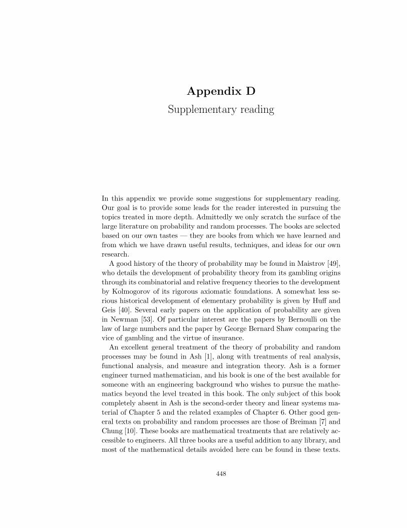
Appendix D

Supplementary reading

In this appendix we provide some suggestions for supplementary reading.

Our goal is to provide some leads for the reader interested in pursuing the

topics treated in more depth. Admittedly we only scratch the surface of the

large literature on probability and random processes. The books are selected

based on our own tastes — they are books from which we have learned and

from which we have drawn useful results, techniques, and ideas for our own

research.

A good history of the theory of probability may be found in Maistrov [49],

who details the development of probability theory from its gambling origins

through its combinatorial and relative frequency theories to the development

by Kolmogorov of its rigorous axiomatic foundations. A somewhat less se-

rious historical development of elementary probability is given by Huff and

Geis [40]. Several early papers on the application of probability are given

in Newman [53]. Of particular interest are the papers by Bernoulli on the

law of large numbers and the paper by George Bernard Shaw comparing the

vice of gambling and the virtue of insurance.

An excellent general treatment of the theory of probability and random

processes may be found in Ash [1], along with treatments of real analysis,

functional analysis, and measure and integration theory. Ash is a former

engineer turned mathematician, and his book is one of the best available for

someone with an engineering background who wishes to pursue the mathe-

matics beyond the level treated in this book. The only subject of this book

completely absent in Ash is the second-order theory and linear systems ma-

terial of Chapter 5 and the related examples of Chapter 6. Other good gen-

eral texts on probability and random processes are those of Breiman [7] and

Chung [10]. These books are mathematical treatments that are relatively ac-

cessible to engineers. All three books are a useful addition to any library, and

most of the mathematical details avoided here can be found in these texts.

448

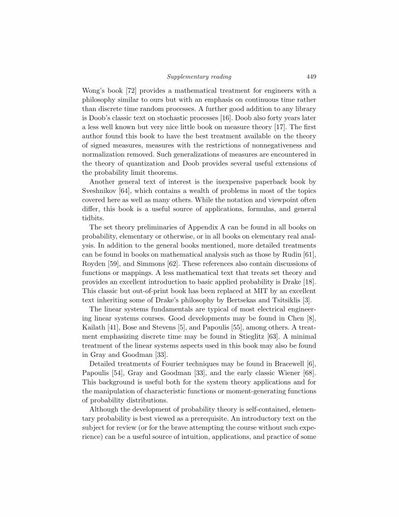
Supplementary reading 449

Wong’s book [72] provides a mathematical treatment for engineers with a

philosophy similar to ours but with an emphasis on continuous time rather

than discrete time random processes. A further good addition to any library

is Doob’s classic text on stochastic processes [16]. Doob also forty years later

a less well known but very nice little book on measure theory [17]. The first

author found this book to have the best treatment available on the theory

of signed measures, measures with the restrictions of nonnegativeness and

normalization removed. Such generalizations of measures are encountered in

the theory of quantization and Doob provides several useful extensions of

the probability limit theorems.

Another general text of interest is the inexpensive paperback book by

Sveshnikov [64], which contains a wealth of problems in most of the topics

covered here as well as many others. While the notation and viewpoint often

differ, this book is a useful source of applications, formulas, and general

tidbits.

The set theory preliminaries of Appendix A can be found in all books on

probability, elementary or otherwise, or in all books on elementary real anal-

ysis. In addition to the general books mentioned, more detailed treatments

can be found in books on mathematical analysis such as those by Rudin [61],

Royden [59], and Simmons [62]. These references also contain discussions of

functions or mappings. A less mathematical text that treats set theory and

provides an excellent introduction to basic applied probability is Drake [18].

This classic but out-of-print book has been replaced at MIT by an excellent

text inheriting some of Drake’s philosophy by Bertsekas and Tsitsiklis [3].

The linear systems fundamentals are typical of most electrical engineer-

ing linear systems courses. Good developments may be found in Chen [8],

Kailath [41], Bose and Stevens [5], and Papoulis [55], among others. A treat-

ment emphasizing discrete time may be found in Stieglitz [63]. A minimal

treatment of the linear systems aspects used in this book may also be found

in Gray and Goodman [33].

Detailed treatments of Fourier techniques may be found in Bracewell [6],

Papoulis [54], Gray and Goodman [33], and the early classic Wiener [68].

This background is useful both for the system theory applications and for

the manipulation of characteristic functions or moment-generating functions

of probability distributions.

Although the development of probability theory is self-contained, elemen-

tary probability is best viewed as a prerequisite. An introductory text on the

subject for review (or for the brave attempting the course without such expe-

rience) can be a useful source of intuition, applications, and practice of some

450 Supplementary reading

of the basic ideas. Two books that admirably fill this function are Drake [18]

and the classic introductory text by two of the primary contributors to the

early development of probability theory, Gnedenko and Khinchine [30]. The

more complete text by Gnedenko [29] also provides a useful backup text.

A virtual encyclopedia of basic probability, including a wealth of examples,

distributions, and computations, may be found in Feller [22].

The axiomatic foundations of probability theory presented in Chapter 2

were developed by Kolmogorov and first published in 1933. (See the En-

glish translation [44].) Although not the only theory of probability (see,

e.g., Fine [23] for a survey of other approaches), it has become the stan-

dard approach to the analysis of random systems. The general references

cited previously provide good additional material for the basic development

of probability spaces, measures, Lebesgue integration, and expectation. The

reader interested in probing more deeply into the mathematics is referred to

the classics by Halmos [37] and Loeve [47].

As observed in Chapter 4, instead of beginning with axioms of probability

and deriving the properties of expectation, one can go the other way and

begin with axioms of expectation or integration and derive the properties of

probability. Some texts treat measure and integration theory in this order,

e.g., Asplund and Bungart [2]. A nice paperback book treating probabil-

ity and random processes from this viewpoint in a manner accessible for

engineers is that by Whittle [67].

A detailed and quite general development of the Kolmogorov extension

theorem of Chapter 3 may be found in Parthasarathy [56], who treats prob-

ability theory for general metric spaces instead of just Euclidean spaces. The

mathematical level of this book is high, though, and the going can be rough.

It is useful, however, as a reference for very general results of this variety

and for detailed statements of the theorem. A treatment may also be found

in Gray [32].

Good background reading for Chapters 4 and 6 are the book on conver-

gence of random variables by Lukacs [48] and the book on ergodic theory

by Billingsley [4]. The Billingsley book is a real gem for engineers inter-

ested in learning more about the varieties and proofs of ergodic theorems

for discrete time processes. The book also provides nice tutorial reviews on

advanced conditional probability and a variety of other topics. Several proofs

are given for the mean and pointwise ergodic theorems. Most are accessi-

ble given a knowledge of the material of this book plus a knowledge of the

projection theorem of Hilbert space theory. The book also provides insight

into applications of the general formulation of ergodic theory to areas other

Supplementary reading 451

than random process theory. Another nice survey of ergodic theory is that

of Halmos [38].

As discussed in Chapter 6, stationarity and ergodicity are sufficient but

not necessary conditions for the ergodic theorem to hold, that is, for sample

averages to converge. A natural question, then, is what conditions are both

necessary and sufficient. The answer is known for discrete time processes in

the following sense: A process is said to be asymptotically mean stationary

or ams if its process distribution, say m, is such that the limits

limn→∞

1

n

n−1∑

i=0

m(T−iF )

exist for all process events F , where T is the left-shift operation. The limits

trivially exist if the process is stationary. They also exist when they die out

with time and in a variety of other cases. It is known that a process will have

an ergodic theorem in the sense of having all sample averages of bounded

measurements converge if and only if the process is ams [34, 32]. The sample

averages of an ams process will converge to constants with probability one

if and only the process is also ergodic.

Second-order theory of random processes and its application to filter-

ing and estimation form a bread-and-butter topic for engineering applica-

tions and are the subject of numerous good books such as Grenander and

Rosenblatt [35], Cramer and Leadbetter [13], Rozanov [60], Yaglom [73], and

Liptster and Shiryayev [46]. It was pointed out that the theory of weakly

stationary processes is intimately related to the theory of Toeplitz forms

and Toeplitz matrices. An excellent treatment of the topic and its applica-

tions to random processes is given by Grenander and Szego [36]. A more

informal engineering-oriented treatment of Toeplitz matrices can be found

in Gray [31].

It is emphasized in our book that the focus is on discrete time random

processes because of their simplicity. While many of the basic ideas gen-

eralize, the details can become far more complicated, and much additional

mathematical power becomes required. For example, the simple product

sigma fields used here to generate process events are not sufficiently large

to be useful. A simple integral of the process over a finite time window will

not be measurable with respect to the resulting event spaces. Most of the

added difficulties are technical — that is, the natural analogs to the dis-

crete time results may hold, but the technical details of their proof can be

far more complicated. Many excellent texts emphasizing continuous time

random processes are available, but most require a solid foundation in func-

452 Supplementary reading

tional analysis and in measure and integration theory. Perhaps the most

famous and complete treatment is that of Doob [16]. Several of the refer-

ences for second-order theory focus on continuous time random processes, as

do Gikhman and Skorokhod [27], Hida [39], and McKean [51]. Lamperti [45]

presents a clear summary of many facets of continuous time and discrete

time random processes, including second-order theory, ergodic theorems,

and prediction theory.

In Chapter 5 we sketch briefly some basic ideas of Wiener and Kalman

filters as an application of second-order theory. A detailed general devel-

opment of the fundamentals and recent results in this area may be found

in Kailath [42] and the references listed therein. In particular, the classic

development of Wiener [69] is an excellent treatment of the fundamentals of

Wiener filtering.

Of the menagerie of processes considered in the book, most may be found

in the various references already mentioned. The communication modulation

examples may also be found in Gagliardi [24], among others. Compound

Poisson processes are treated in detail in Parzen [57]. There is an extensive

literature on Markov processes and their applications, as examples we cite

Kemeny and Snell [43], Chung [9], Rosenblatt [58], and Dynkin [21].

Perhaps the most notable beast absent from our menagerie of processes is

the class of martingales. If the book and the target class length were longer,

martingales would be the next topic to be added. They were not included

simply because we felt the current content already filled a semester, and we

did not want to expand the book past that goal. An excellent mathematical

treatment for the discrete time case may be found in Neveu [52], and a

readable description of the applications of martingale theory to gambling

may be found in the classic by Dubins and Savage [20].

References

[1] R. B. Ash. Real Analysis and Probability. Academic Press, New York,

1972.

[2] E. Asplund and L. Bungart. A First Course in Integration.

Holt,Rinehart and Winston, New York, 1966.

[3] D. T. Bertsekas and J. N. Tsitsiklis. Introduction to Probability. Athena

Scientific, Boston, 2002.

[4] P. Billingsley. Ergodic Theory and Information. Wiley, New York, 1965.

[5] A. G. Bose and K. N. Stevens. Introductory Network Theory. Harper

& Row, New York, 1965.

[6] R. Bracewell. The Fourier Transform and Its Applications. McGraw-

Hill, New York, 1965.

[7] L. Breiman. Probability. Addison-Wesley, Menlo Park, CA, 1968.

[8] C. T. Chen. Introduction to Linear System Theory. Holt, Rinehart and

Winston, New York, 1970.

[9] K. L. Chung. Markov Chains with Stationary Transition Probabilities.

Springer-Verlag, New York, 1967.

[10] K. L. Chung. A Course in Probability Theory. Academic Press, New

York, 1974.

[11] T. M. Cover, P. Gacs, and R. M. Gray. Kolmogorov’s contributions to

information theory and algorithmic complexity. Ann. Probab., 17:840–

865, 1989.

[12] T. M. Cover and J. A. Thomas. Elements of Information Theory. Wiley,

New York, 1991.

[13] H. Cramer and M. R. Leadbetter. Stationary and Related Stochastic

Processes. Wiley, New York, 1967.

[14] W. B. Davenport and W. L Root. An Introduction to the Theory of

Random Signals and Noise. McGraw-Hill, New York, 1958.

[15] R. L. Dobrushin. The description of random field by means of condi-

453

454 References

tional probabilities and conditions of its regularity. Theory Prob. Appl.,

13:197–224, 1968.

[16] J. L. Doob. Stochastic Processes. Wiley, New York, 1953.

[17] Joseph L. Doob. Measure Theory. Springer-Verlag, New York, 1994.

[18] A. W. Drake. Fundamentals of Applied Probability Theory. McGraw-

Hill, San Francisco, 1967.

[19] R. C. Dubes and A. K. Jain. Random field model in image analysis.

Journal of Applied Statistics, 16:131–164, 1989.

[20] L. E. Dubins and L. J. Savage. Inequalities for Stochastic Processes:

How to Gamble If You Must. Dover, New York, 1976.

[21] E. B. Dynkin. Markov Processes. Springer-Verlag, New York, 1965.

[22] W. Feller. An Introduction to Probability Theory and its Applications,

volume 2. Wiley, New York, 1960. 3rd ed.

[23] T. Fine. Properties of an optimal digital system and applications. IEEE

Trans. Inform. Theory, 10:287–296, Oct 1964.

[24] R. Gagliardi. Introduction to Communications Engineering. Wiley, New

York, 1978.

[25] Karl F. Gauss. Theoria Motus Corporum Coelestium (Theory of the

Motion of the Heavenly Bodies Moving about the Sun in Conic Sec-

tions). Little, Brown, and Co.,, 1987. republished by Dover, 1963.

[26] A. Gersho and R. M. Gray. Vector Quantization and Signal Compres-

sion. Kluwer Academic Publishers, Boston, 1992.

[27] I. I. Gikhman and A. V. Skorokhod. Introduction to the Theory of

Random Processes. Saunders, Philadelphia, 1965.

[28] James Gleick. Chaos: making a new science. Penguin Books, 1987.

[29] B. V. Gnedenko. The Theory of Probability. Chelsea, New York, 1963.

Translated from the Russian by B. D. Seckler.

[30] B. V. Gnedenko and A. Ya. Khinchine. An Elementary Introduction to

the Theory of Probability. Dover, New York, 1962. Translated from the

5th Russian edition by L. F. Boron.

[31] R. M. Gray. Toeplitz and Circulent Matrices. ISL technical report 6504–

1, Stanford University Information Systems Laboratory, 1977. Revised

version is available online at http:/ee.stanford.edu/˜gray/toeplitz.html.

[32] R. M. Gray. Probability, Random Processes, and Ergodic Properties.

Springer-Verlag, New York, 1988. http://ee.stanford.edu/arp.html.

[33] R. M. Gray and J. G. Goodman. Fourier Transforms. Kluwer Academic

Publishers, Boston, Mass., 1995.

[34] R. M. Gray and J. C. Kieffer. Asymptotically mean stationary mea-

sures. Ann. Probab., 8:962–973, 1980.

References 455

[35] U. Grenander and M. Rosenblatt. Statistical Analysis of Stationary

Time Series. Wiley, New York, 1957.

[36] U. Grenander and G. Szego. Toeplitz Forms and Their Applications.

University of California Press, Berkeley and Los Angeles, 1958.

[37] P. R. Halmos. Measure Theory. Van Nostrand Reinhold, New York,

1950.

[38] P. R. Halmos. Lectures on Ergodic Theory. Chelsea, New York, 1956.

[39] T. Hida. Stationary Stochastic Processes. Princeton University Press,

Princeton, NJ, 1970.

[40] D. Huff and I. Geis. How to Take a Chance. W. W. Norton, New York,

1959.

[41] T. Kailath. Linear Systems. Prentice-Hall, Englewood Cliffs, NJ, 1980.

[42] T. Kailath. Lectures on Wiener and Kalman Filtering. CISM Courses

and Lectures No. 140. Springer-Verlag, New York, 1981.

[43] J. G. Kemeny and J. L. Snell. Finite Markov Chains. D. Van Nostrand,

Princeton, NJ, 1960.

[44] A. N. Kolmogorov. Foundations of the Theory of Probability. Chelsea,

New York, 1950.

[45] J. Lamperti. Stochastic Processes: A Survey of the Mathematical The-

ory. Springer-Verlag, New York, 1977.

[46] R. S. Liptser and A. N. Shiryayev. Statistics of Random Processes.

Springer-Verlag, New York, 1977. Translated by A. B. Aries.

[47] M. Loeve. Probability Theory. D. Van Nostrand, Princeton, NJ, 1963.

Third Edition.

[48] E. Lukacs. Stochastic Convergence. Heath, Lexington, MA, 1968.

[49] L. E. Maistrov. Probability Theory: A Historical Sketch. Academic

Press, New York, 1974. Translated by S. Kotz.

[50] J. D. Markel and A. H. Gray, Jr. Linear Prediction of Speech. Springer-

Verlag, New York, 1976.

[51] H. P. McKean, Jr. Stochastic Integrals. Academic Press, New York,

1969.

[52] J. Neveu. Discrete-Parameter Martingales. North-Holland, New York,

1975. Translated by T. P. Speed.

[53] J. R. Newman. The World of Mathematics, volume 3. Simon & Schus-

ter, New York, 1956.

[54] A. Papoulis. The Fourier Integral and Its Applications. McGraw-Hill,

New York, 1962.

[55] A. Papoulis. Signal Analysis. McGraw-Hill, New York, 1977.

[56] K. R. Parthasarathy. Probability Measures on Metric Spaces. Academic

456 References

Press, New York, 1967.

[57] E. Parzen. Stochastic Processes. Holden Day, San Francisco, 1962.

[58] M. Rosenblatt. Markov Processes: Structure and Asymptotic Behavior.

Springer-Verlag, New York, 1971.

[59] H. L. Royden. Real Analysis. Macmillan, London, 1968.

[60] Yu. A. Rozanov. Stationary Random Processes. Holden Day, San Fran-

cisco, 1967. Translated by A. Feinstein.

[61] W. Rudin. Principles of Mathematical Analysis. McGraw-Hill, New

York, 1964.

[62] G. F. Simmons. Introduction to Topology and Modern Analysis.

McGraw-Hill, New York, 1963.

[63] K. Steiglitz. An Introduction to Discrete Systems. Wiley, New York,

1974.

[64] A. A. Sveshnikov. Problems in Probability Theory, Mathematical Statis-

tics,and Theory of Random Functions. Dover, New York, 1968.

[65] Peter Swerling. A proposed stagewise differential correction procedure

for satellite tracking and prediction. Technical Report P-1292, Rand

Corporation, January 1958.

[66] P. Whittle. On stationary processes in the plane,. Biometrika, 41,:434–

449, 1954.

[67] P. Whittle. Probability. Penguin Books, Middlesex, 1970.

[68] N. Wiener. The Fourier Integral and Certain of Its Applications. Cam-

bridge University Press, New York, 1933.

[69] N. Wiener. Time Series: Extrapolation,Interpolation,and Smoothing

of Stationary Time Series with Engineering Applications. MIT Press,

Cambridge, MA, 1966.

[70] N. Wiener and R. E. A. C. Paley. Fourier Transforms in the Complex

Domain. American Mathematics Society Coll. Pub., Providence, RI,

1934.

[71] Chee Son Won and Robert M. Gray. Stochastic Image Process-

ing. Information Technology: Transmission, Processing, and Storage.

Kluwer/Plenum, New York, 2004.

[72] E. Wong. Introduction to Random Processes. Springer-Verlag, New

York, 1983.

[73] A. M. Yaglom. An Introduction to the Theory of Stationary Random

Functions. Prentice-Hall, Englewood Cliffs, NJ, 1962. Translated by R.

A. Silverman.

Index

L2, 304Φ-function, xiv, 62δ-response, 99, 276, 430

Cesaro mean, 98

absolute moment, 55, 189centralized, 189

abstract space, 411addition, 305

modulo 2, xiv, 133additive Gaussian noise, 138additive noise, 135

continuous, 137discrete, 135

additivity, 17, 42countable, 42finite, 17, 42

affine, 203, 216, 222affine function, 221algebra, 23almost everywhere, 107alphabet, 102

continuous, 114discrete, 113mixed, 114

amplitudecontinuous, 114discrete, 113

amplitude modulation (AM), 295ams, see asymptotically mean stationaryarea, 10arithmetic average, 98ARMA, see autoregressive moving-averageasymptotic equipartition property, 267asymptotically mean stationary (ams), 451asymptotically uncorrelated, 255, 257Atal, Bishnu S., 220autocorrelation function, 228autocorrelation matrix, 223autoregressive, 289, 378

binary, 159autoregressive filter, 366

autoregressive moving-average (ARMA), 367autoregressive moving-average process, 368autoregressive random process, 368average, 182

probabilistic, 46statistical, 46

average power, 284axioms of probability, 17, 24

Balakrishnan, A. B., 298Banach space, 308baseband noise, 299Bayes risk, 134Bayes’ rule, 129, 131, 134Bernoulli process, 91, 157binary autoregressive filter, 354binary detection, 142binary filter, 353binary Markov process, 158, 290binary pmf, 47binary random variable, 193binomial coefficient, 48, 446binomial counting process, 161, 162, 369binomial pmf, 47, 446binomial theorem, 164bit, 181Bochner’s theorem, 285Bonferroni inequality, 75Borel field, xiii, 35, 36Borel sets, 36Borel space, 54Borel–Cantelli lemma, 245, 246Bose–Einstein distribution, 401Brownian motion, 233

calculus of probability, 102Cartesian product, 28categorical space, 412Cauchy pdf, 258Cauchy sequence, 307Cauchy–Schwarz inequality, 201, 242, 262, 306,

309causal filter, 431

457

458 Index

cdf, see cumulative distribution functioncentral limit theorem, 194, 231, 233chain rule, 129, 160channel

noisy, 133with additive noise, 402

chaotic, 179characteristic function, xiv, 135, 145, 146, 149,

192Gaussian random variable, 150Gaussian random vector, 151multivariable, 202

Chernoff inequality, 248chi-squared, 111classification

statistical, 134closed interval, 27coin flipping, 18, 48, 83, 122collectively exhaustive, 422comb filter, 350complement, 416complementary Phi function, xivcomplementation, 416complete, 75complete metric space, 307complete the square, 124, 138, 139, 150completeness of L2, 308completion, 75complex-valued random variables, 304complex-valued random vector, 112composite function, 97composite processes, 386compound process, 385conditional differential entropy, 267conditional distribution, 127

continuous, 129discrete, 128

conditional expectation, 206conditional mean, 140conditional pmf, 128conditional probability, 70

nonelementary, 167, 168conditional probability density function, 72conditional probability mass function, 72conditional variance, 140consistency, 15, 88, 118, 119consistent distributions, 88, 156continuity, 43

from above, 44from below, 44

continuous function, 423continuous probability spaces, 54continuous space, 27continuous time, 113convergence

almost everywhere, 237almost surely, 237in distribution, 233, 236in mean square, 237in probability, 237, 238in quadratic mean, 237

mean square, 237of correlation, 308of expectation, 308of random variables, 236pointwise, 237w.p. 1, 237with probability one, 237, 245

convolution, 428discrete, 136modulo 2, 136sum, 136

coordinate function, 97correlation, 198correlation coefficient, 124, 131, 269cosine identity, 295cost, 134countable, 421counting process, 161

binomial, 161covariance, 200covariance function, 228covariance matrix, 202cross-correlation, 262, 336cross-covariance, 209cross-spectral density, 336cumulative distribution function (cdf), xiv, 79,

104, 117

dc response, 279decision rule, 133

maximum a-posteriori, 134decreasing sets, 32delta

Dirac, 64, 283Kronecker, 434

DeMorgan’s law, 30, 420density

mass, 10dependent random variables, 89derived distribution, 20, 85, 108detection, 133

maximum a-posteriori (MAP), 142determinant, 204dice, 22, 122difference

symmetric, 418differential entropy, 205differentiating random processes, 315Dirac delta, 64, 283directly given, 20discrete spaces, 27discrete time, 90, 113discrete time impulse response, 430discrete time signals, 28disjoint sets, 16, 417, 422distance, 76, 305distribution, xiv, 64, 84, 102, 115

conditional, 127convergence in, 233infinitely divisible, 234joint, 119

Index 459

marginal, 119stable, 269

domain, 423domain of definition, 19dominated convergence theorem, 197dot product, 424double convolution, 282doubly exponential pdf, 447doubly stochastic, 387

eigenfunction, 327eigenvalue, 327, 425eigenvector, 425element, 411elementary events, 22elementary outcomes, 22empty set, xiii, 18, 414equivalent random variables, 85ergodic decomposition, 398ergodic theorems, 182, 185, 255, 257ergodicity, 395error, mean squared, 212estimate

minimum mean squared error (MMSE), 216estimation, 144, 211

linear, 331maximum a posteriori (MAP), 145maximum likelihood (ML), 145minimum mean squared error (MMSE), 212,

215optimal, 214recursive, 340statistical, 144

Euclidean space, 28even function, 187event, 23

elementary, 22event space, xiii, 11, 23, 30

trivial, 26exclusive or, 133expectation, xiv, 7, 46, 54, 182, 184, 186

conditional, 206fundamental theorem of, 190iterated, 207nested, 207

expected value, 185experiment, 6, 11, 17, 25exponential modulation, 387, 388exponential pdf, 61, 447exponential random variable, 187

field, 23Borel, xiii

filter, 158autoregressive, 366binary, 353comb, 350finite impulse response, 277, 364infinite impulse response, 364linear, 428moving-average, 364

transversal, 364filtered Poisson process, 408finest-grain, 27finite additivity, 17finite impulse response (FIR), 277, 364, 430FIR, see finite impulse responseFM, see frequency modulationFourier analysis, 277Fourier series, 319Fourier transform, 146, 149, 193, 278, 282,

302, 365frequency domain, 283frequency modulation (FM), 388function

affine, 221continuous, 423identity, 46linear, 221measurable, 95odd, 188of random variables, 188, 195Toeplitz, 250

functions, 423orthogonal, 328

fundamental theorem of expectation, 190

Galois field, 132Gamma pdf, 447Gauss–Markov process, 380Gaussian

jointly, 209multidimensional, 67

Gaussian pdf, 61, 193, 447Gaussian random process, 157, 229, 315, 381Gaussian random vectors, 151, 152, 209generating event spaces, 36geometric pmf, 446geometric random variable, 187Gibbs random field, 399Gram–Schmidt, 329

half-open interval, 27Hamming weight, 54, 158hard limiter, 96Hermitian, 219, 230, 425–427hidden Markov model, 166Hilbert space, 308

identically distributed, 85identity function, 46identity mapping, 85iid, see independent identically distributedIIR, see infinite impulse responseimage, 423impulse response, 427increasing sets, 32increments, 371

independent, 372stationary, 372

independence, 68, 124, 125linear, 198

460 Index

independent and stationary increments, 370independent identically distributed (iid), 91,

126, 127, 156independent increments, 372independent random variables, 125, 199independent stationary increment (isi), 372indexed family, 113indicator function, xiv, 15, 45, 191induction, 49inequality

Tchebychev, 239infinite

countably, 421infinite impluse response (IIR), 430infinite impulse response (IIR) filter, 364infinitely divisible, 234inner product, 307, 424inner product space, 307input event, 93input signal, ix, 2, 83integer sets, xivintegration

Lebesgue, 56, 443Riemann, 16, 56, 57, 310Stieltjes, 105, 191

integrator, discrete time, 369intersection, 416, 417interval, xiii, 27, 415

closed, xiii, 415half-closed, 415half-open, 415open, xiii, 415

intervals, 35inverse image, 84, 423inverse image formula, 85isi, see independent stationary increments, 372Itakura, Fumitada, 220iterated expectation, 207, 208

Jacobian, 111joint distribution, 119jointly Gaussian, 151

Kalman–Bucy filtering, 340Karhunen–Loeve expansion, 327Kolmogorov extension theorem, 92, 156Kolmogorov, A. N., 22, 42, 92Kronecker delta, 434Kronecker delta response, 99, 430

Laplace transform, 149, 193Laplacian pdf, 60, 447law of large numbers, 7, 182, 185

strong, 249Lebesgue integral, 9, 58, 443Lebesgue integration, 56limit in the mean, 238limits

of probabilities, 43of sets, 32

linear estimation, 218, 331

linear function, 221linear functional equation, 374linear least squares error, 220linear models, 364, 368linear modulation, 292linear system, 427linearity of expectation, 196linearly filtered uncorrelated processes, 286linearly independent, 329Lloyd–Max quantizer, 272logistic pdf, 447low band noise, 299

MAP, see maximum a-posteriorimapping, 423

one-to-one, 423onto, 423

marginal pmf, 88Markov chain, 161Markov inequality, 239Markov process, 158, 161, 163, 166

continuous time, 377Markov random field, 399martingale, 271, 452mass, 10matrix, 424

Hermitian, 425max function, 172maximum a-posteriori (MAP)

decision rule, 134detector, 142estimation, 145

maximum likelihood (ML) estimation, 145mean, 46, 55, 98, 185

conditional, 140mean ergodic theorem, 243, 255, 257mean function, 157mean square convergence, 237, 304mean square integral, 310, 311mean square sampling theorem, 324mean squared error (MSE), 214mean squared error (MSE), 212mean value theorem, 104mean vector, 201measurable function, 95measurable space, 24measure theory, 10measure, probability, 41memoryless, 158Mercer’s theorem, 330metric, 76, 305metric space, 305min function, 172minimum distance, 143minimum mean squared error (MMSE)

estimate, 216mixture, 68, 106, 397

probability, 67process, 387

ML, see maximum likelihoodMMSE, see minimum mean squared error

Index 461

modulationnonlinear, 269

modulo 2 arithmetic, xiv, 132, 158moment, 189, 192

kth, 46, 55absolute, 55, 189centralized, 55, 189first, 46, 55second, 55, 201

moment-generating function, 193monotone convergence theorem, 197monotonically decreasing, 111monotonically increasing, 111moving-average, 271, 289, 364, 378moving-average filter, 364moving-average random process, 271, 368MSE, see mean squared errormultidimensional pdf’s, 65multidimensional pmf’s, 53multiplication, 305mutually exclusive sets, 16, 417mutually independent, 91

narrow band noise, 299nested expectation, 207nested sets, 32noise

white, 286, 296noisy channel, 133nonempty, 411nonlinear modulation, 269nonnegative definite, 152, 426normed linear space, 305, 306numeric space, 412

odd function, 188one-sided, 28, 90, 427one-step prediction, 216one-to-one mapping, 423onto mapping, 423open interval, 27operation, 144optimal, 346orthogonal, 320orthogonal functions, 328orthogonal random variables, 227, 333orthogonality condition, 347orthogonality principle, 223, 226, 227, 333outer product, 425output event, 93output signal, ix, 2, 83output space, 20

Paley–Wiener criteria, 298Parceval’s theorem, 321partition, 422Pascal’s distribution, 258pdf, see probability density functionphase modulation (PM), 388pixel, 399PM, see frequency modulation

pmf, see probability mass functionpoint, 411pointwise convergence, 237Poisson counting process, 371, 378, 382, 409Poisson pmf, 52, 446positive definite, 67, 124, 152, 219, 426power set, 34power spectral density, 283–285pre-Hilbert space, 307prediction

one-step, 214, 216optimal, 214

preimage, 423probabilistic average, 185probability

a-posteriori, 70a-priori, 70conditional, 70unconditional, 70

probability density function (pdf), xiv, 16, 59,399

k-dimensional, 66Cauchy, 258chi-squared, 111doubly exponential, 60, 447elementary conditional, 72exponential, 60, 61, 447Gamma, 447Gaussian, 60, 61, 447Laplacian, 60, 447logistic, 447multidimensional, 65Rayleigh, 447uniform, 16, 60, 447Weibull, 447

probability mass function (pmf), xiv, 18, 45,399

binary, 47, 446binomial, 47, 446conditional, 72, 128geometric, 446Pascal, 258Poisson, 446product, 122uniform, 47, 446

probability measure, xiv, 11, 17, 24, 41probability of error, 133probability space, 6, 10, 11, 17, 22, 25

complete, 75trivial, 26

probability theory, 10product pmf, 122product space, 27, 38, 414projection, 97pseudo-random, 272pseudo-random number, 21pulse amplitude modulation (PAM), 355

quantization, 155, 177quantizer, 19, 96, 176, 433, 443

462 Index

random field, 399random object, 82random phase process, 155random process, 1, 82, 90, 112, 113

ARMA, 368autoregressive, 368Bernoulli, 157composite, 386counting, 161doubly stochastic, 387Gaussian, 157, 315independent identically distributed (iid), 156independent stationary increment (isi), 372Markov, 158, 166mixture, 387moving-average, 271, 368switched, 387

random rotations, 154random telegraph wave, 388random variables, 6, 20, 46, 54, 82, 83, 93, 94

complex-valued, 112, 304continuous, 108discrete, 108equivalent, 85Gaussian, 95independent, 125, 199mixture, 108orthogonal, 227, 333real-valued, 95, 399

random vector, 82, 86, 112, 113Gaussian, 151, 209iid, 127

random walk, 164, 271range, 19, 423range space, 423Rayleigh distribution , 447rectangles, 40recursive estimation, 340regression, 144regression coefficients, 366relative frequency, 21, 184Riemann integral, 310Riemann integration, 16, 56, 57, 258, 310

sample autocorrelation, 287sample average, 98, 234sample points, 22sample space, xiii, 10, 22, 27sample value, 83sampling expansion, 323sampling function, 97sampling interval, 322sampling theorem

mean square, 324scalar, 305second-order input/output relations, 275second-order moments, 373sequence, 38

Cauchy, 307sequence space, 29set, 414

empty, xiiiuniversal, xiii

set difference, 417set theory, 411sets

decreasing, 32empty, 414increasing, 32nested, 32one-point, 414singleton, 414universal, 411

Shannon, Claude, 267shift, 249sigma-algebra, 23sigma-field, xiii, 11, 23, 30

generated, 36signal, 13, 427

continuous time, 29discrete time, 28

signal processing, ix, 2, 13, 19, 20, 46simple function, 443single-sided, 427singular, 152, 204singular Gaussian distribution, 204sliding average, 400space, 411

Banach, 308continuous, 27empty, 411event, xiiiHilbert, 308inner product, 307metric, 305normed linear, 305pre-Hilbert, 307product, 27, 414trivial, 411

spectrum, 302spinning pointer, 14square root, 219square-integrable, 304stable, 428, 430stable distribution, 269stable filter, 277standard deviation, 201stationarity properties, 249stationary, 252–254

first-order, 250strict sense, 252, 253strictly, 252weakly, 217, 250

stationary increments, 372statistical classification, 132, 134statistical detection, 132statistical estimation, 144Stieltjes integration, 105, 191stochastic process, 1, 113strict stationarity, 252, 253strong law of large numbers, 245, 249subset, 414

Index 463

sum of independent random variables, 149sums of iid random variables, 369superposition, 427switched random process, 387symmetric, 424symmetric difference, 418system, 427

continuous time, 427discrete time, 427linear, 427

tapped delay line, 364Taylor series, 52, 193Tchebychev inequality, 239telescoping sum, 43thermal noise, 21, 392Thevinin’s theorem, 394threshold detector, 143time

continuous, 113discrete, 113

time average, 98, 299time series, 90, 113time-invariant, 428Toeplitz function, 250Toeplitz matrix, 250, 439transform

Fourier, 146, 278Laplace, 149

transpose, 113transversal filter, 364trivial probability space, 26trivial sigma-field, 101two-sided, 28, 427Tyche, 14

uncorrelated, 198, 199, 201, 229, 235asymptotically, 255, 257

uncountable, 421uniform pdf, 16, 47, 60, 447uniform pmf, 446uniform random variable, 187union, 416, 417union bound, 75unit impulse, 64unit pulse response, 99, 430universal set, xiii, 411

variance, 47, 55, 189, 201conditional, 140

vector, 38, 424random, 113

vocoder, 2volume, 10

waveform, 38weak law of large numbers, 243weakly stationary, 217, 250, 279Weibull pdf, 447weight, 10white noise, 286, 296, 331

Wiener process, 290, 369, 371continuous time, 373, 377discrete time, 164

Wiener, Norbert, 5Wiener–Hopf equation, 331, 348