An Introduction to Modern

Econometrics Using Stata

CHRISTOPHER F. BAUMDepartment of Economics

Boston College

A Stata Press PublicationStataCorp LPCollege Station, Texas

Stata Press, 4905 Lakeway Drive, College Station, Texas 77845

Copyright c© 2006 by StataCorp LP

All rights reserved

Typeset in LATEX2ε

Printed in the United States of America

10 9 8 7 6 5 4 3 2 1

ISBN-10: 1-59718-013-0

ISBN-13: 978-1-59718-013-9

This book is protected by copyright. All rights are reserved. No part of this book may be repro-

duced, stored in a retrieval system, or transcribed, in any form or by any means—electronic,

mechanical, photocopying, recording, or otherwise—without the prior written permission of

StataCorp LP.

Stata is a registered trademark of StataCorp LP. LATEX2ε is a trademark of the American

Mathematical Society.

Contents

Illustrations xv

Preface xvii

Notation and typography xix

1 Introduction 1

1.1 An overview of Stata’s distinctive features . . . . . . . . . . . . . . . . 1

1.2 Installing the necessary software . . . . . . . . . . . . . . . . . . . . . . 4

1.3 Installing the support materials . . . . . . . . . . . . . . . . . . . . . . 5

2 Working with economic and financial data in Stata 7

2.1 The basics . . . . . . . . . . . . . . . . . . . . . . . . . . . . . . . . . . 7

2.1.1 The use command . . . . . . . . . . . . . . . . . . . . . . . . . 7

2.1.2 Variable types . . . . . . . . . . . . . . . . . . . . . . . . . . . 8

2.1.3 n and N . . . . . . . . . . . . . . . . . . . . . . . . . . . . . . 9

2.1.4 generate and replace . . . . . . . . . . . . . . . . . . . . . . . . 10

2.1.5 sort and gsort . . . . . . . . . . . . . . . . . . . . . . . . . . . 10

2.1.6 if exp and in range . . . . . . . . . . . . . . . . . . . . . . . . 11

2.1.7 Using if exp with indicator variables . . . . . . . . . . . . . . . 13

2.1.8 Using if exp versus by varlist: with statistical commands . . . 15

2.1.9 Labels and notes . . . . . . . . . . . . . . . . . . . . . . . . . . 17

2.1.10 The varlist . . . . . . . . . . . . . . . . . . . . . . . . . . . . . 20

2.1.11 drop and keep . . . . . . . . . . . . . . . . . . . . . . . . . . . 20

2.1.12 rename and renvars . . . . . . . . . . . . . . . . . . . . . . . . 21

2.1.13 The save command . . . . . . . . . . . . . . . . . . . . . . . . 21

2.1.14 insheet and infile . . . . . . . . . . . . . . . . . . . . . . . . . . 21

viii Contents

2.2 Common data transformations . . . . . . . . . . . . . . . . . . . . . . . 22

2.2.1 The cond() function . . . . . . . . . . . . . . . . . . . . . . . . 22

2.2.2 Recoding discrete and continuous variables . . . . . . . . . . . 23

2.2.3 Handling missing data . . . . . . . . . . . . . . . . . . . . . . 24

mvdecode and mvencode . . . . . . . . . . . . . . . . . . . . . 25

2.2.4 String-to-numeric conversion and vice versa . . . . . . . . . . . 26

2.2.5 Handling dates . . . . . . . . . . . . . . . . . . . . . . . . . . . 27

2.2.6 Some useful functions for generate or replace . . . . . . . . . . 29

2.2.7 The egen command . . . . . . . . . . . . . . . . . . . . . . . . 30

Official egen functions . . . . . . . . . . . . . . . . . . . . . . . 30

egen functions from the user community . . . . . . . . . . . . 31

2.2.8 Computation for by-groups . . . . . . . . . . . . . . . . . . . . 33

2.2.9 Local macros . . . . . . . . . . . . . . . . . . . . . . . . . . . . 36

2.2.10 Looping over variables: forvalues and foreach . . . . . . . . . . 37

2.2.11 Scalars and matrices . . . . . . . . . . . . . . . . . . . . . . . 39

2.2.12 Command syntax and return values . . . . . . . . . . . . . . . 39

3 Organizing and handling economic data 43

3.1 Cross-sectional data and identifier variables . . . . . . . . . . . . . . . 43

3.2 Time-series data . . . . . . . . . . . . . . . . . . . . . . . . . . . . . . . 44

3.2.1 Time-series operators . . . . . . . . . . . . . . . . . . . . . . . 45

3.3 Pooled cross-sectional time-series data . . . . . . . . . . . . . . . . . . 45

3.4 Panel data . . . . . . . . . . . . . . . . . . . . . . . . . . . . . . . . . . 46

3.4.1 Operating on panel data . . . . . . . . . . . . . . . . . . . . . 47

3.5 Tools for manipulating panel data . . . . . . . . . . . . . . . . . . . . . 49

3.5.1 Unbalanced panels and data screening . . . . . . . . . . . . . . 50

3.5.2 Other transforms of panel data . . . . . . . . . . . . . . . . . . 53

3.5.3 Moving-window summary statistics and correlations . . . . . . 53

3.6 Combining cross-sectional and time-series datasets . . . . . . . . . . . . 55

3.7 Creating long-format datasets with append . . . . . . . . . . . . . . . . 56

3.7.1 Using merge to add aggregate characteristics . . . . . . . . . . 57

Contents ix

3.7.2 The dangers of many-to-many merges . . . . . . . . . . . . . . 58

3.8 The reshape command . . . . . . . . . . . . . . . . . . . . . . . . . . . 58

3.8.1 The xpose command . . . . . . . . . . . . . . . . . . . . . . . 62

3.9 Using Stata for reproducible research . . . . . . . . . . . . . . . . . . . 62

3.9.1 Using do-files . . . . . . . . . . . . . . . . . . . . . . . . . . . . 62

3.9.2 Data validation: assert and duplicates . . . . . . . . . . . . . . 63

4 Linear regression 69

4.1 Introduction . . . . . . . . . . . . . . . . . . . . . . . . . . . . . . . . . 69

4.2 Computing linear regression estimates . . . . . . . . . . . . . . . . . . . 70

4.2.1 Regression as a method-of-moments estimator . . . . . . . . . 72

4.2.2 The sampling distribution of regression estimates . . . . . . . 73

4.2.3 Efficiency of the regression estimator . . . . . . . . . . . . . . 74

4.2.4 Numerical identification of the regression estimates . . . . . . 75

4.3 Interpreting regression estimates . . . . . . . . . . . . . . . . . . . . . . 75

4.3.1 Research project: A study of single-family housing prices . . . 76

4.3.2 The ANOVA table: ANOVA F and R-squared . . . . . . . . . 77

4.3.3 Adjusted R-squared . . . . . . . . . . . . . . . . . . . . . . . . 78

4.3.4 The coefficient estimates and beta coefficients . . . . . . . . . 80

4.3.5 Regression without a constant term . . . . . . . . . . . . . . . 81

4.3.6 Recovering estimation results . . . . . . . . . . . . . . . . . . . 82

4.3.7 Detecting collinearity in regression . . . . . . . . . . . . . . . . 84

4.4 Presenting regression estimates . . . . . . . . . . . . . . . . . . . . . . 87

4.4.1 Presenting summary statistics and correlations . . . . . . . . . 90

4.5 Hypothesis tests, linear restrictions, and constrained least squares . . . 91

4.5.1 Wald tests with test . . . . . . . . . . . . . . . . . . . . . . . . 94

4.5.2 Wald tests involving linear combinations of parameters . . . . 96

4.5.3 Joint hypothesis tests . . . . . . . . . . . . . . . . . . . . . . . 98

4.5.4 Testing nonlinear restrictions and forming nonlinear combi-nations . . . . . . . . . . . . . . . . . . . . . . . . . . . . . . . 99

4.5.5 Testing competing (nonnested) models . . . . . . . . . . . . . 100

x Contents

4.6 Computing residuals and predicted values . . . . . . . . . . . . . . . . 102

4.6.1 Computing interval predictions . . . . . . . . . . . . . . . . . . 103

4.7 Computing marginal effects . . . . . . . . . . . . . . . . . . . . . . . . 107

4.A Appendix: Regression as a least-squares estimator . . . . . . . . . . . . 112

4.B Appendix: The large-sample VCE for linear regression . . . . . . . . . 113

5 Specifying the functional form 115

5.1 Introduction . . . . . . . . . . . . . . . . . . . . . . . . . . . . . . . . . 115

5.2 Specification error . . . . . . . . . . . . . . . . . . . . . . . . . . . . . . 115

5.2.1 Omitting relevant variables from the model . . . . . . . . . . . 116

Specifying dynamics in time-series regression models . . . . . 117

5.2.2 Graphically analyzing regression data . . . . . . . . . . . . . . 117

5.2.3 Added-variable plots . . . . . . . . . . . . . . . . . . . . . . . 119

5.2.4 Including irrelevant variables in the model . . . . . . . . . . . 121

5.2.5 The asymmetry of specification error . . . . . . . . . . . . . . 121

5.2.6 Misspecification of the functional form . . . . . . . . . . . . . 122

5.2.7 Ramsey’s RESET . . . . . . . . . . . . . . . . . . . . . . . . . 122

5.2.8 Specification plots . . . . . . . . . . . . . . . . . . . . . . . . . 124

5.2.9 Specification and interaction terms . . . . . . . . . . . . . . . 125

5.2.10 Outlier statistics and measures of leverage . . . . . . . . . . . 126

The DFITS statistic . . . . . . . . . . . . . . . . . . . . . . . . 128

The DFBETA statistic . . . . . . . . . . . . . . . . . . . . . . 130

5.3 Endogeneity and measurement error . . . . . . . . . . . . . . . . . . . . 132

6 Regression with non-i.i.d. errors 133

6.1 The generalized linear regression model . . . . . . . . . . . . . . . . . . 134

6.1.1 Types of deviations from i.i.d. errors . . . . . . . . . . . . . . 134

6.1.2 The robust estimator of the VCE . . . . . . . . . . . . . . . . 136

6.1.3 The cluster estimator of the VCE . . . . . . . . . . . . . . . . 138

6.1.4 The Newey–West estimator of the VCE . . . . . . . . . . . . . 139

6.1.5 The generalized least-squares estimator . . . . . . . . . . . . . 142

The FGLS estimator . . . . . . . . . . . . . . . . . . . . . . . 143

Contents xi

6.2 Heteroskedasticity in the error distribution . . . . . . . . . . . . . . . . 143

6.2.1 Heteroskedasticity related to scale . . . . . . . . . . . . . . . . 144

Testing for heteroskedasticity related to scale . . . . . . . . . . 145

FGLS estimation . . . . . . . . . . . . . . . . . . . . . . . . . 147

6.2.2 Heteroskedasticity between groups of observations . . . . . . . 149

Testing for heteroskedasticity between groups of observations . 150

FGLS estimation . . . . . . . . . . . . . . . . . . . . . . . . . 151

6.2.3 Heteroskedasticity in grouped data . . . . . . . . . . . . . . . 152

FGLS estimation . . . . . . . . . . . . . . . . . . . . . . . . . 153

6.3 Serial correlation in the error distribution . . . . . . . . . . . . . . . . . 154

6.3.1 Testing for serial correlation . . . . . . . . . . . . . . . . . . . 155

6.3.2 FGLS estimation with serial correlation . . . . . . . . . . . . . 159

7 Regression with indicator variables 161

7.1 Testing for significance of a qualitative factor . . . . . . . . . . . . . . 161

7.1.1 Regression with one qualitative measure . . . . . . . . . . . . 162

7.1.2 Regression with two qualitative measures . . . . . . . . . . . . 165

Interaction effects . . . . . . . . . . . . . . . . . . . . . . . . . 167

7.2 Regression with qualitative and quantitative factors . . . . . . . . . . . 168

Testing for slope differences . . . . . . . . . . . . . . . . . . . 170

7.3 Seasonal adjustment with indicator variables . . . . . . . . . . . . . . . 174

7.4 Testing for structural stability and structural change . . . . . . . . . . 179

7.4.1 Constraints of continuity and differentiability . . . . . . . . . . 179

7.4.2 Structural change in a time-series model . . . . . . . . . . . . 183

8 Instrumental-variables estimators 185

8.1 Introduction . . . . . . . . . . . . . . . . . . . . . . . . . . . . . . . . . 185

8.2 Endogeneity in economic relationships . . . . . . . . . . . . . . . . . . 185

8.3 2SLS . . . . . . . . . . . . . . . . . . . . . . . . . . . . . . . . . . . . . 188

8.4 The ivreg command . . . . . . . . . . . . . . . . . . . . . . . . . . . . . 189

8.5 Identification and tests of overidentifying restrictions . . . . . . . . . . 190

8.6 Computing IV estimates . . . . . . . . . . . . . . . . . . . . . . . . . . 192

xii Contents

8.7 ivreg2 and GMM estimation . . . . . . . . . . . . . . . . . . . . . . . . 194

8.7.1 The GMM estimator . . . . . . . . . . . . . . . . . . . . . . . 195

8.7.2 GMM in a homoskedastic context . . . . . . . . . . . . . . . . 196

8.7.3 GMM and heteroskedasticity-consistent standard errors . . . . 197

8.7.4 GMM and clustering . . . . . . . . . . . . . . . . . . . . . . . 198

8.7.5 GMM and HAC standard errors . . . . . . . . . . . . . . . . . 199

8.8 Testing overidentifying restrictions in GMM . . . . . . . . . . . . . . . 200

8.8.1 Testing a subset of the overidentifying restrictions in GMM . . 201

8.9 Testing for heteroskedasticity in the IV context . . . . . . . . . . . . . 205

8.10 Testing the relevance of instruments . . . . . . . . . . . . . . . . . . . . 207

8.11 Durbin–Wu–Hausman tests for endogeneity in IV estimation . . . . . . 211

8.A Appendix: Omitted-variables bias . . . . . . . . . . . . . . . . . . . . . 216

8.B Appendix: Measurement error . . . . . . . . . . . . . . . . . . . . . . . 216

8.B.1 Solving errors-in-variables problems . . . . . . . . . . . . . . . 218

9 Panel-data models 219

9.1 FE and RE models . . . . . . . . . . . . . . . . . . . . . . . . . . . . . 220

9.1.1 One-way FE . . . . . . . . . . . . . . . . . . . . . . . . . . . . 221

9.1.2 Time effects and two-way FE . . . . . . . . . . . . . . . . . . . 224

9.1.3 The between estimator . . . . . . . . . . . . . . . . . . . . . . 226

9.1.4 One-way RE . . . . . . . . . . . . . . . . . . . . . . . . . . . . 227

9.1.5 Testing the appropriateness of RE . . . . . . . . . . . . . . . . 230

9.1.6 Prediction from one-way FE and RE . . . . . . . . . . . . . . 231

9.2 IV models for panel data . . . . . . . . . . . . . . . . . . . . . . . . . . 232

9.3 Dynamic panel-data models . . . . . . . . . . . . . . . . . . . . . . . . 232

9.4 Seemingly unrelated regression models . . . . . . . . . . . . . . . . . . 236

9.4.1 SUR with identical regressors . . . . . . . . . . . . . . . . . . 241

9.5 Moving-window regression estimates . . . . . . . . . . . . . . . . . . . . 242

10 Models of discrete and limited dependent variables 247

10.1 Binomial logit and probit models . . . . . . . . . . . . . . . . . . . . . 247

10.1.1 The latent-variable approach . . . . . . . . . . . . . . . . . . . 248

Contents xiii

10.1.2 Marginal effects and predictions . . . . . . . . . . . . . . . . . 250

Binomial probit . . . . . . . . . . . . . . . . . . . . . . . . . . 251

Binomial logit and grouped logit . . . . . . . . . . . . . . . . . 253

10.1.3 Evaluating specification and goodness of fit . . . . . . . . . . . 254

10.2 Ordered logit and probit models . . . . . . . . . . . . . . . . . . . . . . 256

10.3 Truncated regression and tobit models . . . . . . . . . . . . . . . . . . 259

10.3.1 Truncation . . . . . . . . . . . . . . . . . . . . . . . . . . . . . 259

10.3.2 Censoring . . . . . . . . . . . . . . . . . . . . . . . . . . . . . . 262

10.4 Incidental truncation and sample-selection models . . . . . . . . . . . . 266

10.5 Bivariate probit and probit with selection . . . . . . . . . . . . . . . . . 271

10.5.1 Binomial probit with selection . . . . . . . . . . . . . . . . . . 272

A Getting the data into Stata 277

A.1 Inputting data from ASCII text files and spreadsheets . . . . . . . . . 277

A.1.1 Handling text files . . . . . . . . . . . . . . . . . . . . . . . . . 278

Free format versus fixed format . . . . . . . . . . . . . . . . . 278

The insheet command . . . . . . . . . . . . . . . . . . . . . . . 280

A.1.2 Accessing data stored in spreadsheets . . . . . . . . . . . . . . 281

A.1.3 Fixed-format data files . . . . . . . . . . . . . . . . . . . . . . 281

A.2 Importing data from other package formats . . . . . . . . . . . . . . . . 286

B The basics of Stata programming 289

B.1 Local and global macros . . . . . . . . . . . . . . . . . . . . . . . . . . 290

B.1.1 Global macros . . . . . . . . . . . . . . . . . . . . . . . . . . . 293

B.1.2 Extended macro functions and list functions . . . . . . . . . . 293

B.2 Scalars . . . . . . . . . . . . . . . . . . . . . . . . . . . . . . . . . . . . 294

B.3 Loop constructs . . . . . . . . . . . . . . . . . . . . . . . . . . . . . . . 295

B.3.1 foreach . . . . . . . . . . . . . . . . . . . . . . . . . . . . . . . 297

B.4 Matrices . . . . . . . . . . . . . . . . . . . . . . . . . . . . . . . . . . . 299

B.5 return and ereturn . . . . . . . . . . . . . . . . . . . . . . . . . . . . . 301

B.5.1 ereturn list . . . . . . . . . . . . . . . . . . . . . . . . . . . . . 305

xiv Contents

B.6 The program and syntax statements . . . . . . . . . . . . . . . . . . . . 307

B.7 Using Mata functions in Stata programs . . . . . . . . . . . . . . . . . 313

References 321

Author index 329

Subject index 333

Preface

This book is a concise guide for applied researchers in economics and finance to learnbasic econometrics and use Stata with examples using typical datasets analyzed ineconomics. Readers should be familiar with applied statistics at the level of a simplelinear regression (ordinary least squares, or OLS) model and its algebraic representation,equivalent to the level of an undergraduate statistics/econometrics course sequence.1

The book also uses some multivariate calculus (partial derivatives) and linear algebra.

I presume that the reader is familiar with Stata’s windowed interface and with thebasics of data input, data transformation, and descriptive statistics. Readers shouldconsult the appropriate Getting Started with Stata manual if review is needed. Mean-while, readers already comfortable interacting with Stata should feel free to skip tochapter 4, where the discussion of econometrics begins in earnest.

In any research project, a great deal of the effort is involved with the preparationof the data specified as part of an econometric model. While the primary focus of thebook is placed upon applied econometric practice, we must consider the considerablechallenges that many researchers face in moving from their original data sources tothe form needed in an econometric model—or even that needed to provide appropriatetabulations and graphs for the project. Accordingly, Chapter 2 focuses on the detailsof data management and several tools available in Stata to ensure that the appropriatetransformations are accomplished accurately and efficiently. If you are familiar withthese aspects of Stata usage, you should feel free to skim this material, perhaps returningto it to refresh your understanding of Stata usage. Likewise, Chapter 3 is devoted to adiscussion of the organization of economic and financial data, and the Stata commandsneeded to reorganize data among the several forms of organization (cross section, timeseries, pooled, panel/longitudinal, etc.) If you are eager to begin with the econometricsof linear regression, skim this chapter, noting its content for future reference.

Chapter 4 begins the econometric content of the book and presents the most widelyused tool for econometric analysis: the multiple linear regression model applied tocontinuous variables. The chapter also discusses how to interpret and present regressionestimates and discusses the logic of hypothesis tests and linear and nonlinear restrictions.The last section of the chapter considers residuals, predicted values, and marginal effects.

Applying the regression model depends on some assumptions that real datasetsoften violate. Chapter 5 discusses how the crucial zero-conditional-mean assumptionof the errors may be violated in the presence of specification error. The chapter also

1. Two excellent texts at this level are Wooldridge (2006) and Stock and Watson (2006).

xviii Preface

discusses statistical and graphical techniques for detecting specification error. Chapter 6discusses other assumptions that may be violated, such as the assumption of independentand identically distributed (i.i.d.) errors, and presents the generalized linear regressionmodel. It also explains how to diagnose and correct the two most important departuresfrom i.i.d., heteroskedasticity and serial correlation.

Chapter 7 discusses using indicator variables or dummy variables in the linear re-gression models containing both quantitative and qualitative factors, models with in-teraction effects, and models of structural change.

Many regression models in applied economics violate the zero-conditional-mean as-sumption of the errors because they simultaneously determine the response variable andone or more regressors or because of measurement error in the regressors. No matterthe cause, OLS techniques will no longer generate unbiased and consistent estimates, soyou must use instrumental-variables (IV) techniques instead. Chapter 8 presents theIV estimator and its generalized method-of-moments counterpart along with tests fordetermining the need for IV techniques.

Chapter 9 applies models to panel or longitudinal data that have both cross-sectionaland time-series dimensions. Extensions of the regression model allow you to take ad-vantage of the rich information in panel data, accounting for the heterogeneity in bothpanel unit and time dimensions.

Many econometric applications model categorical and limited dependent variables:a binary outcome, such as a purchase decision, or a constrained response such as theamount spent, which combines the decision whether to purchase with the decision ofhow much to spend, conditional on purchasing. Because linear regression techniquesare generally not appropriate for modeling these outcomes, chapter 10 presents severallimited-dependent-variable estimators available in Stata.

The appendices discuss techniques for importing external data into Stata and explainbasic Stata programming. Although you can use Stata without doing any programming,learning how to program in Stata can help you save a lot of time and effort. You shouldalso learn to generate reproducible results by using do-files that you can document,archive, and rerun. Following Stata’s guidelines will make your do-files shorter andeasier to maintain and modify.

4 Linear regression

This chapter presents the most widely used tool in applied economics: the linear regres-sion model, which relates a set of continuous variables to a continuous outcome. Theexplanatory variables in a regression model often include one or more binary or indica-tor variables; see chapter 7. Likewise, many models seek to explain a binary responsevariable as a function of a set of factors, which linear regression does not handle well.Chapter 10 discusses several forms of that model, including those in which the responsevariable is limited but not binary.

4.1 Introduction

This chapter discusses multiple regression in the context of a prototype economic re-search project. To carry out such a research project, we must

1. lay out a research framework—or economic model—that lets us specify the ques-tions of interest and defines how we will interpret the empirical results;

2. find a dataset containing empirical counterparts to the quantities specified in theeconomic model;

3. use exploratory data analysis to familiarize ourselves with the data and identifyoutliers, extreme values, and the like;

4. fit the model and use specification analysis to determine the adequacy of theexplanatory factors and their functional form;

5. conduct statistical inference (given satisfactory findings from specification analy-sis) on the research questions posed by the model; and

6. analyze the findings from hypothesis testing and the success of the model in termsof predictions and marginal effects. On the basis of these findings, we may haveto return to one of the earlier stages to reevaluate the dataset and its specificationand functional form.

Section 2 reviews the basic regression analysis theory on which regression point andinterval estimates are based. Section 3 introduces a prototype economic research projectstudying the determinants of communities’ single-family housing prices and discusses thevarious components of Stata’s results from fitting a regression model of housing prices.Section 4 discusses how to transform Stata’s estimation results into publication-qualitytables. Section 5 discusses hypothesis testing and estimation subject to constraints on

69

70 Chapter 4 Linear regression

the parameters. Section 6 deals with computing residuals and predicted values. Thelast section discusses computing marginal effects. In the following chapters, we take upviolations of the assumptions on which regression estimates are based.

4.2 Computing linear regression estimates

The linear regression model is the most widely used econometric model and the baselineagainst which all others are compared. It specifies the conditional mean of a responsevariable y as a linear function of k independent variables

E [y | x1, x2, . . . , xk] = β1x1 + β2x2 + · · · + βkxk

Given values for the βs, which are fixed parameters, the linear regression model predictsthe average value of y in the population for different values of x1, x2, . . . , xk.

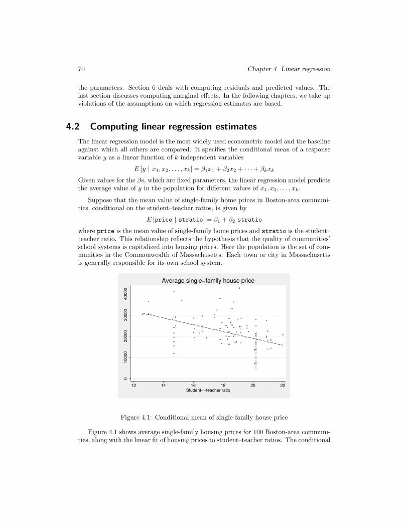
Suppose that the mean value of single-family home prices in Boston-area communi-ties, conditional on the student–teacher ratios, is given by

E [price | stratio] = β1 + β2 stratio

where price is the mean value of single-family home prices and stratio is the student–teacher ratio. This relationship reflects the hypothesis that the quality of communities’school systems is capitalized into housing prices. Here the population is the set of com-munities in the Commonwealth of Massachusetts. Each town or city in Massachusettsis generally responsible for its own school system.

010000

20000

30000

40000

12 14 16 18 20 22Student−−teacher ratio

Average single−family house price

Figure 4.1: Conditional mean of single-family house price

Figure 4.1 shows average single-family housing prices for 100 Boston-area communi-ties, along with the linear fit of housing prices to student–teacher ratios. The conditional

4.2 Computing linear regression estimates 71

mean of price for each value of stratio is shown by the appropriate point on the line.As theory predicts, the mean house price conditional on the student–teacher ratio isinversely related to that ratio. Communities with more crowded schools are consideredless desirable. Of course, this relationship between house price and the student–teacherratio must be considered ceteris paribus: all other factors that might affect the priceof the house are held constant when we evaluate the effect of a measure of communityschools’ quality on the house price.

In working with economic data, we do not know the population values of β1, β2, . . . ,βk. We work with a sample of N observations of data from that population. Using theinformation in this sample, we must

1. obtain good estimates of the coefficients (β1, β2, . . . , βk);

2. determine how much our coefficient estimates would change if we were given an-other sample from the same population;

3. decide whether there is enough evidence to rule out some values for some of thecoefficients (β1, β2, . . . , βk); and

4. use our estimated (β1, β2, . . . , βk) to interpret the model.

To obtain estimates of the coefficients, some assumptions must be made about theprocess that generated the data. I discuss those assumptions below and describe what Imean by good estimates. Before performing steps 2–4, I check whether the data supportthese assumptions by using a process known as specification analysis.

If we have a cross-sectional sample from the population, the linear regression modelfor each observation in the sample has the form

yi = β1 + β2xi,2 + β3xi,3 + · · · + βkxi,k + ui

for each observation in the sample i = 1, 2, . . . , N . The u process is a stochastic distur-bance, representing the net effect of all other unobservable factors that might influencey. The variance of its distribution, σ2

u, is an unknown population parameter to beestimated along with the β parameters. We assume that N > k: to conduct statis-tical inference, there must be more observations in the sample than parameters to beestimated. In practice, N must be much larger than k.

We can write the linear regression model in matrix form as

y = Xβ + u (4.1)

where X is an N × k matrix of sample values.1

This population regression function specifies that a set of k regressors in X and thestochastic disturbance u are the determinants of the response variable (or regressand)

1. Some textbooks use k in this context to refer to the number of slope parameters rather than thenumber of columns of X. That will explain the deviations in the formulas given below; where I writek some authors write (k + 1).

72 Chapter 4 Linear regression

y. We usually assume that the model contains a constant term, so x1 is understood toequal one for each observation.

The key assumption in the linear regression model involves the relationship in thepopulation between the regressors x and u.2 We may rewrite (4.1) as

u = y − xβ

We assume thatE [u | x] = 0 (4.2)

i.e., that the u process has a zero-conditional mean. This assumption is that the un-observed factors involved in the regression function are not related systematically tothe observed factors. This approach to the regression model lets us consider both non-stochastic and stochastic regressors in X without distinction, as long as they satisfy theassumption of (4.2).3

4.2.1 Regression as a method-of-moments estimator

We may use the zero-conditional-mean assumption shown in (4.2) to define a method-of-moments estimator of the regression function. Method-of-moments estimators aredefined by moment conditions that are assumed to hold for the population moments.When we replace the unobservable population moments by their sample counterparts,we derive feasible estimators of the model’s parameters. The zero-conditional-meanassumption gives rise to a set of k moment conditions, one for each x. In particular, thezero-conditional-mean assumption implies that each regressor is uncorrelated with u.4

E[x′u] = 0

E[x′(y − xβ)] = 0 (4.3)

Substituting calculated moments from our sample into the expression and replacing theunknown coefficients β with estimated values β in (4.3) yields the ordinary least squares(OLS) estimator

X′y − X′Xβ = 0

β = (X′X)−1X′y (4.4)

We may use β to calculate the regression residuals:

u = y − Xβ

2. x is a vector of random variables and u is scalar random variable. In (4.1), X is a matrix ofrealizations of the random vector x, u and y are vectors of realizations of the scalar random variablesu and y.

3. Chapter 8 discusses how to use the instrumental-variables estimator when the zero-conditional-mean assumption is encountered.

4. The assumption of zero-conditional mean is stronger than that of a zero covariance, because co-variance considers only linear relationships between the random variables.

4.2.2 The sampling distribution of regression estimates 73

Given the solution for the vector β, the additional parameter of the regression prob-lem σ2

u—the population variance of the stochastic disturbance—may be estimated as afunction of the regression residuals ui

s2 =

∑Ni=1 u

2i

N − k=

u′u

N − k(4.5)

where (N−k) are the residual degrees of freedom of the regression problem. The positivesquare root of s2 is often termed the standard error of regression, or root mean squarederror. Stata uses the latter term and displays s as Root MSE.

The method of moments is not the only approach for deriving the linear regressionestimator of (4.4), which is the well-known formula from which the OLS estimator isderived.5

4.2.2 The sampling distribution of regression estimates

The OLS estimator β is a vector of random variables because it is a function of therandom variable y, which in turn is a function of the stochastic disturbance u. The OLS

estimator takes on different values for each sample of N observations drawn from thepopulation. Because we often have only one sample to work with, we may be unsure ofthe usefulness of the estimates from that sample. The estimates are the realizations ofthe random vector β from the sampling distribution of the OLS estimator. To evaluatethe precision of a given vector of estimates β, we use the sampling distribution of theregression estimator.

To learn more about the sampling distribution of the OLS estimator, we must makefurther assumptions about the distribution of the stochastic disturbance ui. In clas-sical statistics, the ui were assumed to be independent draws from the same normaldistribution. The modern approach to econometrics drops the normality assumptionand simply assumes that the ui are independent draws from an identical distribution(i.i.d.).6

Using the normality assumption, we were able to derive the exact finite-sampledistribution of the OLS estimator. In contrast, under the i.i.d. assumption, we must uselarge-sample theory to derive the sampling distribution of the OLS estimator. Basically,large-sample theory supposes that the sample size N becomes infinitely large. Since noreal sample is infinitely large, these methods only approximate the sampling distributionof the OLS estimator in finite samples. With a few hundred observations or more,the large-sample approximation works well, so these methods work well with appliedeconomic datasets.

5. The treatment here is similar to that of Wooldridge (2006). See Stock and Watson (2006) andappendix 4.A for a derivation based on minimizing the squared-prediction errors.

6. Both frameworks also assume that the (constant) variance of the u process is finite. Formally, i.i.d.stands for independently and identically distributed.

74 Chapter 4 Linear regression

Although large-sample theory is more abstract than finite-sample methods, it im-poses weaker assumptions on the data-generating process. We will use large-sampletheory to define “good” estimators and to evaluate the precision of the estimates pro-duced from a given sample.

In large samples, consistency means that as N goes to ∞, the estimates will convergeto their respective population parameters. Roughly speaking, if the probability that theestimator produces estimates arbitrarily close to the population values goes to one asthe sample size increases to infinity, the estimator is said to be consistent.

The sampling distribution of an estimator describes the set of estimates producedwhen that estimator is applied to repeated samples from the underlying population.You can use the sampling distribution of an estimator to evaluate the precision of agiven set of estimates and to statistically test whether the population parameters takeon certain values.

Large-sample theory shows that the sampling distribution of the OLS estimator isapproximately normal.7 Specifically, when the ui are i.i.d. with finite variance σ2

u, the

OLS estimator β has a large-sample normal distribution with mean β and varianceσ2

uQ−1, where Q−1 is the variance–covariance matrix of X in the population. The

variance–covariance of the estimator, σ2uQ

−1, is also referred to as a VCE. Because itis unknown, we need a consistent estimator of the VCE. Although neither σ2

u nor Q−1

is actually known, we can use consistent estimators of them to construct a consistentestimator of σ2

uQ−1. Given that s2 consistently estimates σ2

u and 1/N(X′X) consistentlyestimates Q, s2(X′X)−1 is a VCE of the OLS estimator.8

4.2.3 Efficiency of the regression estimator

Under the assumption of i.i.d. errors, the Gauss–Markov theorem holds. Among linear,unbiased estimators, the OLS estimator has the smallest sampling variance, or the great-est precision.9 In that sense, it is best, so that “ordinary least squares is BLUE” (thebest linear unbiased estimator) for the parameters of the regression model. If we con-sider only unbiased estimators that are linear in the parameters, we cannot find a moreefficient estimator. The property of efficiency refers to the precision of the estimator. Ifestimator A has a smaller sampling variance than estimator B, estimator A is said tobe relatively efficient. The Gauss–Markov theorem states that OLS is relatively efficient

7. More precisely, the distribution of the OLS estimator converges to a normal distribution. Althoughappendix B provides some details, in the text I will simply refer to the “approximate” or “large-sample”normal distribution. See Wooldridge (2006) for an introduction to large-sample theory.

8. At first glance, you might think that the expression for the VCE should be multiplied by 1/N , butthis assumption is incorrect. As discussed in appendix B, because the OLS estimator is consistent, itis converging to the constant vector of population parameters at the rate 1/

√N , implying that the

variance of the OLS estimator is going to zero as the sample size gets larger. Large-sample theorycompensates for this effect in how it standardizes the estimator. The loss of the 1/N term in theestimator of the VCE is a product of this standardization.

9. For a formal presentation of the Gauss–Markov theorem, see any econometrics text, e.g., Wooldridge(2006, 108–109). The OLS estimator is said to be “unbiased” because E[bβ] = β.

4.3 Interpreting regression estimates 75

versus all other linear, unbiased estimators of the parameterization model. However,this statement rests upon the hypotheses of an appropriately specified model and ani.i.d. disturbance process with a zero-conditional mean, as specified in (4.2).

4.2.4 Numerical identification of the regression estimates

As in (4.4) above, the solution to the regression problem involves a set of k moment

conditions, or equations to be jointly solved for the k parameter estimates β1, β2, . . . , βk.When will these k parameter estimates be uniquely determined, or numerically iden-tified? We must have more sample observations than parameters to be estimated, orN > k. That condition is not sufficient, though. For the simple “two-variable” regres-sion model yi = β1 +β2xi,2 +ui, Var[x2] must be greater than 0. If there is no variationin x2, the data do not provide sufficient information to determine estimates of β1 andβ2.

In multiple regression with many regressors, XN×k must be a matrix of full columnrank k, which implies two things. First, only one column of X can take on a constantvalue, so each of the other regressors must have a positive sample variance. Second,there are no exact linear dependencies among the columns of the matrix X. The as-sumption that X is of full column rank is often stated as “(X′X) is of full rank” or“(X′X) is nonsingular (or invertible).” If the matrix of regressors X contains k linearlyindependent columns, the cross-product matrix (X′X) will have rank k, its inverse willexist, and the parameters β1, . . . , βk in (4.4) will be numerically identified.10 If nu-merical identification fails, the sample does not contain enough information for us touse the regression estimator on the model as it is specified. That model may be validas a description of the data-generating process, but the particular sample may lackthe necessary information to generate a regressor matrix of full column rank. Then wemust either respecify the model or acquire another sample that contains the informationneeded to uniquely determine the regression estimates.

4.3 Interpreting regression estimates

This section illustrates using regression by an example from a prototype research projectand discusses how Stata presents regression estimates. We then discuss how to recoverthe information displayed in Stata’s estimation results for further computations withinyour program and how to combine this information with other estimates to presentthem in a table. The last subsection considers problems of numerical identification, orcollinearity, that may appear when you are estimating the regression equation.

10. When computing infinite precision, we must be concerned with numerical singularity and a com-puter program’s ability to reliably invert a matrix regardless of whether it is analytically invertible. Aswe discuss in section 4.3.7, computationally near-linear dependencies among the columns of X shouldbe avoided.

76 Chapter 4 Linear regression

4.3.1 Research project: A study of single-family housing prices

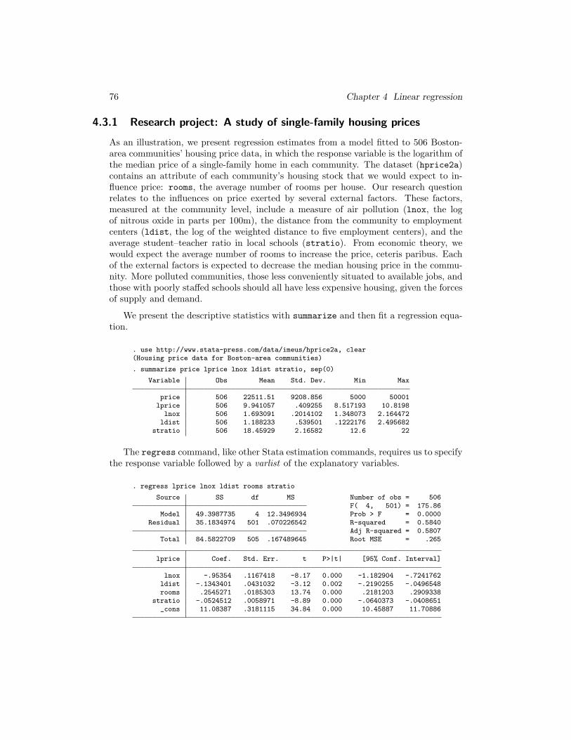
As an illustration, we present regression estimates from a model fitted to 506 Boston-area communities’ housing price data, in which the response variable is the logarithm ofthe median price of a single-family home in each community. The dataset (hprice2a)contains an attribute of each community’s housing stock that we would expect to in-fluence price: rooms, the average number of rooms per house. Our research questionrelates to the influences on price exerted by several external factors. These factors,measured at the community level, include a measure of air pollution (lnox, the logof nitrous oxide in parts per 100m), the distance from the community to employmentcenters (ldist, the log of the weighted distance to five employment centers), and theaverage student–teacher ratio in local schools (stratio). From economic theory, wewould expect the average number of rooms to increase the price, ceteris paribus. Eachof the external factors is expected to decrease the median housing price in the commu-nity. More polluted communities, those less conveniently situated to available jobs, andthose with poorly staffed schools should all have less expensive housing, given the forcesof supply and demand.

We present the descriptive statistics with summarize and then fit a regression equa-tion.

. use http://www.stata-press.com/data/imeus/hprice2a, clear(Housing price data for Boston-area communities)

. summarize price lprice lnox ldist stratio, sep(0)

Variable Obs Mean Std. Dev. Min Max

price 506 22511.51 9208.856 5000 50001lprice 506 9.941057 .409255 8.517193 10.8198

lnox 506 1.693091 .2014102 1.348073 2.164472ldist 506 1.188233 .539501 .1222176 2.495682

stratio 506 18.45929 2.16582 12.6 22

The regress command, like other Stata estimation commands, requires us to specifythe response variable followed by a varlist of the explanatory variables.

. regress lprice lnox ldist rooms stratio

Source SS df MS Number of obs = 506F( 4, 501) = 175.86

Model 49.3987735 4 12.3496934 Prob > F = 0.0000Residual 35.1834974 501 .070226542 R-squared = 0.5840

Adj R-squared = 0.5807Total 84.5822709 505 .167489645 Root MSE = .265

lprice Coef. Std. Err. t P>|t| [95% Conf. Interval]

lnox -.95354 .1167418 -8.17 0.000 -1.182904 -.7241762ldist -.1343401 .0431032 -3.12 0.002 -.2190255 -.0496548rooms .2545271 .0185303 13.74 0.000 .2181203 .2909338

stratio -.0524512 .0058971 -8.89 0.000 -.0640373 -.0408651_cons 11.08387 .3181115 34.84 0.000 10.45887 11.70886

4.3.2 The ANOVA table: ANOVA F and R-squared 77

The header of the regression output describes the overall model estimates, whereasthe table presents the point estimates, their precision, and their interval estimates.

4.3.2 The ANOVA table: ANOVA F and R-squared

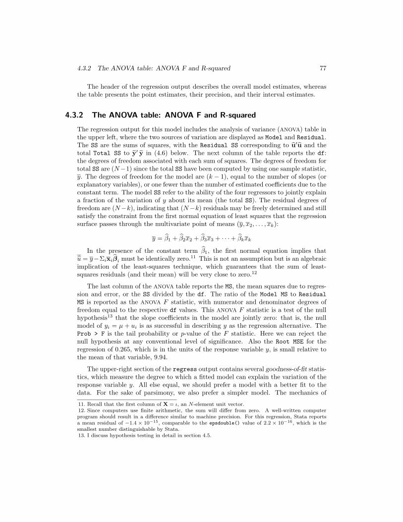
The regression output for this model includes the analysis of variance (ANOVA) table inthe upper left, where the two sources of variation are displayed as Model and Residual.The SS are the sums of squares, with the Residual SS corresponding to u′u and thetotal Total SS to y′ y in (4.6) below. The next column of the table reports the df:the degrees of freedom associated with each sum of squares. The degrees of freedom fortotal SS are (N−1) since the total SS have been computed by using one sample statistic,y. The degrees of freedom for the model are (k − 1), equal to the number of slopes (orexplanatory variables), or one fewer than the number of estimated coefficients due to theconstant term. The model SS refer to the ability of the four regressors to jointly explaina fraction of the variation of y about its mean (the total SS). The residual degrees offreedom are (N−k), indicating that (N−k) residuals may be freely determined and stillsatisfy the constraint from the first normal equation of least squares that the regressionsurface passes through the multivariate point of means (y, x2, . . . , xk):

y = β1 + β2x2 + β3x3 + · · · + βkxk

In the presence of the constant term β1, the first normal equation implies thatu = y−Σixiβi must be identically zero.11 This is not an assumption but is an algebraicimplication of the least-squares technique, which guarantees that the sum of least-squares residuals (and their mean) will be very close to zero.12

The last column of the ANOVA table reports the MS, the mean squares due to regres-sion and error, or the SS divided by the df. The ratio of the Model MS to Residual

MS is reported as the ANOVA F statistic, with numerator and denominator degrees offreedom equal to the respective df values. This ANOVA F statistic is a test of the nullhypothesis13 that the slope coefficients in the model are jointly zero: that is, the nullmodel of yi = µ + ui is as successful in describing y as the regression alternative. TheProb > F is the tail probability or p-value of the F statistic. Here we can reject thenull hypothesis at any conventional level of significance. Also the Root MSE for theregression of 0.265, which is in the units of the response variable y, is small relative tothe mean of that variable, 9.94.

The upper-right section of the regress output contains several goodness-of-fit statis-tics, which measure the degree to which a fitted model can explain the variation of theresponse variable y. All else equal, we should prefer a model with a better fit to thedata. For the sake of parsimony, we also prefer a simpler model. The mechanics of

11. Recall that the first column of X = ι, an N -element unit vector.12. Since computers use finite arithmetic, the sum will differ from zero. A well-written computerprogram should result in a difference similar to machine precision. For this regression, Stata reportsa mean residual of −1.4 × 10−15, comparable to the epsdouble() value of 2.2 × 10−16, which is thesmallest number distinguishable by Stata.13. I discuss hypothesis testing in detail in section 4.5.

78 Chapter 4 Linear regression

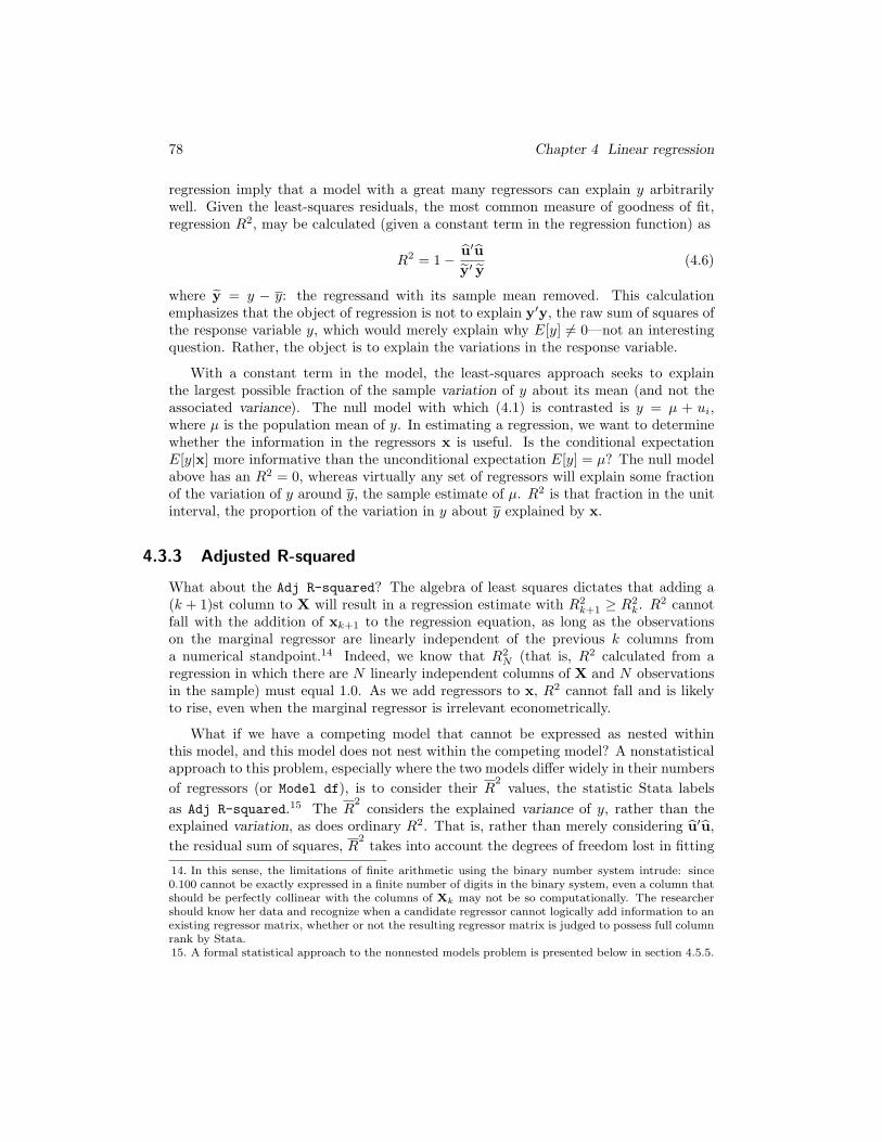
regression imply that a model with a great many regressors can explain y arbitrarilywell. Given the least-squares residuals, the most common measure of goodness of fit,regression R2, may be calculated (given a constant term in the regression function) as

R2 = 1 − u′u

y′ y(4.6)

where y = y − y: the regressand with its sample mean removed. This calculationemphasizes that the object of regression is not to explain y′y, the raw sum of squares ofthe response variable y, which would merely explain why E[y] 6= 0—not an interestingquestion. Rather, the object is to explain the variations in the response variable.

With a constant term in the model, the least-squares approach seeks to explainthe largest possible fraction of the sample variation of y about its mean (and not theassociated variance). The null model with which (4.1) is contrasted is y = µ + ui,where µ is the population mean of y. In estimating a regression, we want to determinewhether the information in the regressors x is useful. Is the conditional expectationE[y|x] more informative than the unconditional expectation E[y] = µ? The null modelabove has an R2 = 0, whereas virtually any set of regressors will explain some fractionof the variation of y around y, the sample estimate of µ. R2 is that fraction in the unitinterval, the proportion of the variation in y about y explained by x.

4.3.3 Adjusted R-squared

What about the Adj R-squared? The algebra of least squares dictates that adding a(k + 1)st column to X will result in a regression estimate with R2

k+1 ≥ R2k. R2 cannot

fall with the addition of xk+1 to the regression equation, as long as the observationson the marginal regressor are linearly independent of the previous k columns froma numerical standpoint.14 Indeed, we know that R2

N (that is, R2 calculated from aregression in which there are N linearly independent columns of X and N observationsin the sample) must equal 1.0. As we add regressors to x, R2 cannot fall and is likelyto rise, even when the marginal regressor is irrelevant econometrically.

What if we have a competing model that cannot be expressed as nested withinthis model, and this model does not nest within the competing model? A nonstatisticalapproach to this problem, especially where the two models differ widely in their numbers

of regressors (or Model df), is to consider their R2

values, the statistic Stata labels

as Adj R-squared.15 The R2

considers the explained variance of y, rather than theexplained variation, as does ordinary R2. That is, rather than merely considering u′u,

the residual sum of squares, R2

takes into account the degrees of freedom lost in fitting

14. In this sense, the limitations of finite arithmetic using the binary number system intrude: since0.100 cannot be exactly expressed in a finite number of digits in the binary system, even a column thatshould be perfectly collinear with the columns of Xk may not be so computationally. The researchershould know her data and recognize when a candidate regressor cannot logically add information to anexisting regressor matrix, whether or not the resulting regressor matrix is judged to possess full columnrank by Stata.15. A formal statistical approach to the nonnested models problem is presented below in section 4.5.5.

4.3.3 Adjusted R-squared 79

the model and scales u′u by (N−k) rather than N .16 R2

can be expressed as a correctedversion of R2 in which the degrees-of-freedom adjustments are made, penalizing a modelwith more regressors for its loss of parsimony:

R2

= 1 − u′u/(N − k)

y′ y/(N − 1)= 1 − (1 −R2)

N − 1

N − k

If an irrelevant regressor is added to a model, R2 cannot fall and will probably

rise, but R2

will rise if the benefit of that regressor (reduced variance of the residuals)

exceeds the cost of including it in the model: 1 degree of freedom.17 Therefore, R2

can fall when a more elaborate model is considered, and indeed it is not bounded by

zero. Algebraically, R2

must be less than R2 since (N − 1)/(N − k) > 1 for any Xmatrix and cannot be interpreted as the “proportion of variation of y”, as can R2 in the

presence of a constant term. Nevertheless, you can use R2

to informally compare modelswith the same response variable but differing specifications. You can also compare theequations’ s2 values (labeled Root MSE in Stata’s output) in units of the dependentvariable to judge nonnested specifications.

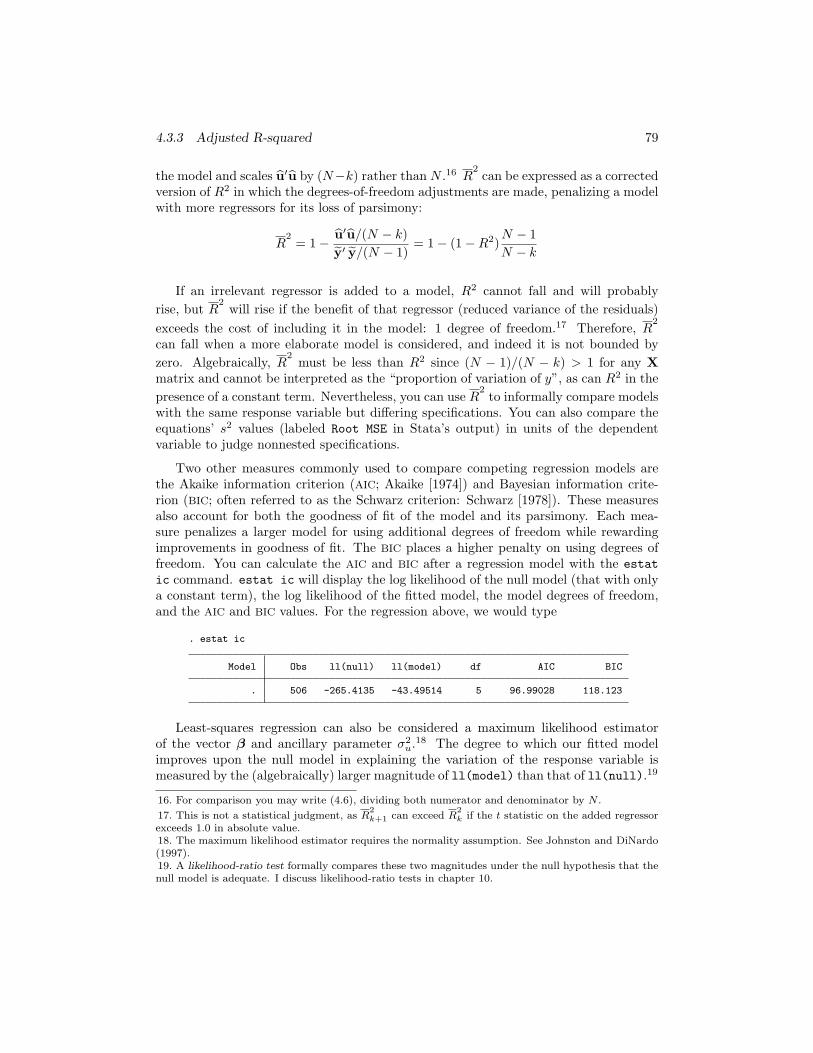
Two other measures commonly used to compare competing regression models arethe Akaike information criterion (AIC; Akaike [1974]) and Bayesian information crite-rion (BIC; often referred to as the Schwarz criterion: Schwarz [1978]). These measuresalso account for both the goodness of fit of the model and its parsimony. Each mea-sure penalizes a larger model for using additional degrees of freedom while rewardingimprovements in goodness of fit. The BIC places a higher penalty on using degrees offreedom. You can calculate the AIC and BIC after a regression model with the estat

ic command. estat ic will display the log likelihood of the null model (that with onlya constant term), the log likelihood of the fitted model, the model degrees of freedom,and the AIC and BIC values. For the regression above, we would type

. estat ic

Model Obs ll(null) ll(model) df AIC BIC

. 506 -265.4135 -43.49514 5 96.99028 118.123

Least-squares regression can also be considered a maximum likelihood estimatorof the vector β and ancillary parameter σ2

u.18 The degree to which our fitted modelimproves upon the null model in explaining the variation of the response variable ismeasured by the (algebraically) larger magnitude of ll(model) than that of ll(null).19

16. For comparison you may write (4.6), dividing both numerator and denominator by N .

17. This is not a statistical judgment, as R2

k+1 can exceed R2

k if the t statistic on the added regressorexceeds 1.0 in absolute value.18. The maximum likelihood estimator requires the normality assumption. See Johnston and DiNardo(1997).19. A likelihood-ratio test formally compares these two magnitudes under the null hypothesis that thenull model is adequate. I discuss likelihood-ratio tests in chapter 10.

80 Chapter 4 Linear regression

4.3.4 The coefficient estimates and beta coefficients

Below the ANOVA table and summary statistics, Stata reports the β coefficient esti-mates, along with their estimated standard errors, t statistics, and the associated p-values labeled P>|t|: that is, the tail probability for a two-tailed test on the hypothesisH0: βj = 0.20 The last two columns display an estimated confidence interval, with limitsdefined by the current setting of level. You can use the level() option on regress

(or other estimation commands) to specify a particular level. After performing the esti-mation (e.g., with the default 95% level), you can redisplay the regression results with,for instance, regress, level(90). You can change the default level (see [R] level)for the session or permanently with set level #

[, permanently

].

Economic researchers often express regressors or response variables in logarithms.21

A model in which the response variable is the log of the original series and the regressorsare in levels is termed a log-linear (or single-log) model. The rough approximation thatlog(1 + x) ≃ x for reasonably small x is used to interpret the regression coefficients.These coefficients are also the semielasticities of y with respect to x, measuring theresponse of y in percentage terms to a unit change in x. When logarithms are usedfor both the response variable and regressors, we have the double-log model. In thismodel, the coefficients are themselves elasticities of y with respect to each x. The mostcelebrated example of a double-log model is the Cobb–Douglas production function,q = alαkβeǫ, which we can estimate by linear regression by taking logs of q, l, and k.

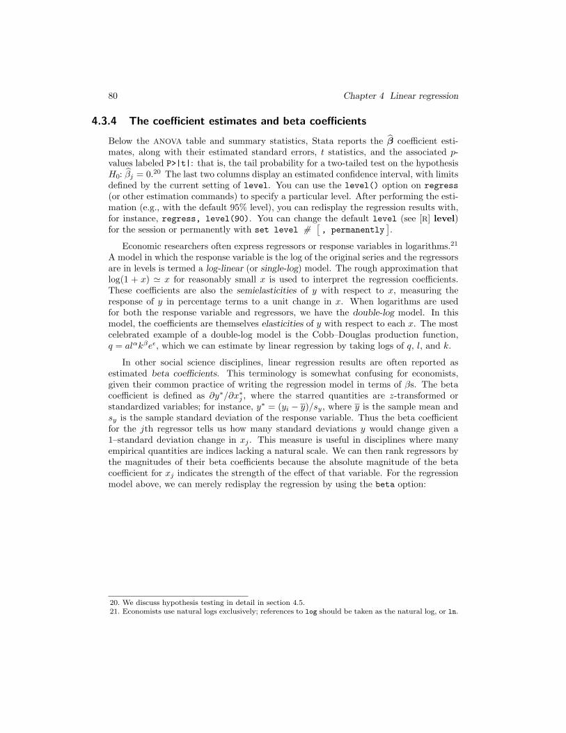
In other social science disciplines, linear regression results are often reported asestimated beta coefficients. This terminology is somewhat confusing for economists,given their common practice of writing the regression model in terms of βs. The betacoefficient is defined as ∂y∗/∂x∗j , where the starred quantities are z-transformed orstandardized variables; for instance, y∗ = (yi − y)/sy, where y is the sample mean andsy is the sample standard deviation of the response variable. Thus the beta coefficientfor the jth regressor tells us how many standard deviations y would change given a1–standard deviation change in xj . This measure is useful in disciplines where manyempirical quantities are indices lacking a natural scale. We can then rank regressors bythe magnitudes of their beta coefficients because the absolute magnitude of the betacoefficient for xj indicates the strength of the effect of that variable. For the regressionmodel above, we can merely redisplay the regression by using the beta option:

20. We discuss hypothesis testing in detail in section 4.5.21. Economists use natural logs exclusively; references to log should be taken as the natural log, or ln.

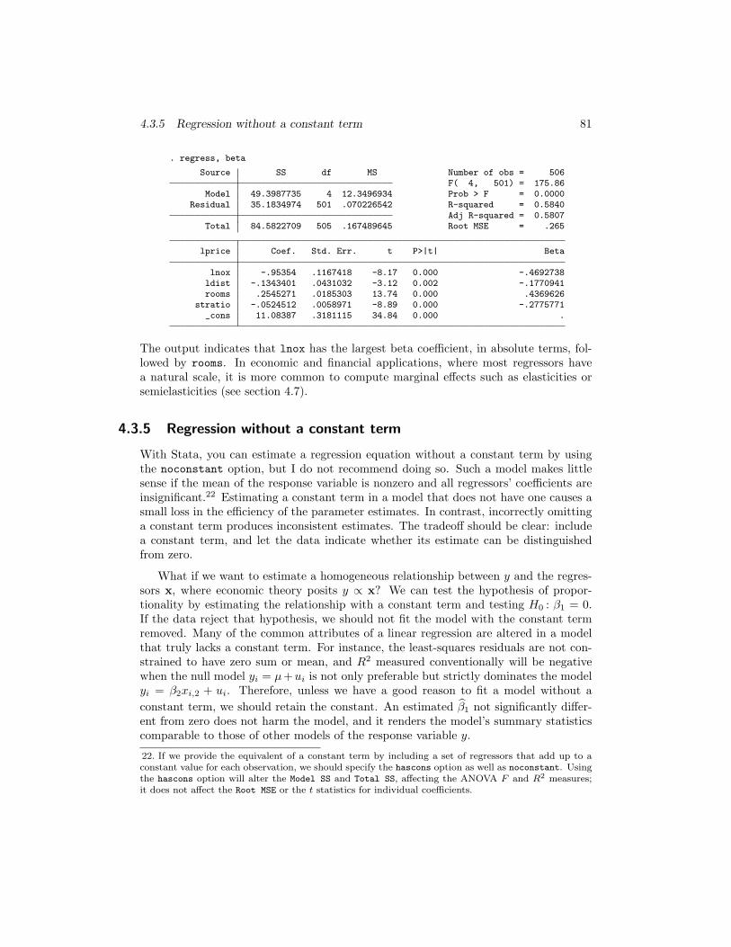
4.3.5 Regression without a constant term 81

. regress, beta

Source SS df MS Number of obs = 506F( 4, 501) = 175.86

Model 49.3987735 4 12.3496934 Prob > F = 0.0000Residual 35.1834974 501 .070226542 R-squared = 0.5840

Adj R-squared = 0.5807Total 84.5822709 505 .167489645 Root MSE = .265

lprice Coef. Std. Err. t P>|t| Beta

lnox -.95354 .1167418 -8.17 0.000 -.4692738ldist -.1343401 .0431032 -3.12 0.002 -.1770941rooms .2545271 .0185303 13.74 0.000 .4369626

stratio -.0524512 .0058971 -8.89 0.000 -.2775771_cons 11.08387 .3181115 34.84 0.000 .

The output indicates that lnox has the largest beta coefficient, in absolute terms, fol-lowed by rooms. In economic and financial applications, where most regressors havea natural scale, it is more common to compute marginal effects such as elasticities orsemielasticities (see section 4.7).

4.3.5 Regression without a constant term

With Stata, you can estimate a regression equation without a constant term by usingthe noconstant option, but I do not recommend doing so. Such a model makes littlesense if the mean of the response variable is nonzero and all regressors’ coefficients areinsignificant.22 Estimating a constant term in a model that does not have one causes asmall loss in the efficiency of the parameter estimates. In contrast, incorrectly omittinga constant term produces inconsistent estimates. The tradeoff should be clear: includea constant term, and let the data indicate whether its estimate can be distinguishedfrom zero.

What if we want to estimate a homogeneous relationship between y and the regres-sors x, where economic theory posits y ∝ x? We can test the hypothesis of propor-tionality by estimating the relationship with a constant term and testing H0 : β1 = 0.If the data reject that hypothesis, we should not fit the model with the constant termremoved. Many of the common attributes of a linear regression are altered in a modelthat truly lacks a constant term. For instance, the least-squares residuals are not con-strained to have zero sum or mean, and R2 measured conventionally will be negativewhen the null model yi = µ+ui is not only preferable but strictly dominates the modelyi = β2xi,2 + ui. Therefore, unless we have a good reason to fit a model without a

constant term, we should retain the constant. An estimated β1 not significantly differ-ent from zero does not harm the model, and it renders the model’s summary statisticscomparable to those of other models of the response variable y.

22. If we provide the equivalent of a constant term by including a set of regressors that add up to aconstant value for each observation, we should specify the hascons option as well as noconstant. Usingthe hascons option will alter the Model SS and Total SS, affecting the ANOVA F and R2 measures;it does not affect the Root MSE or the t statistics for individual coefficients.