An extension of Turan’s inequality for

ultraspherical polynomials∗

Geno Nikolov † Veronika Pillwein ‡

Abstract

Let pm(x) = P(λ)m (x)/P

(λ)m (1) be the m-th ultraspherical polynomial

normalized by pm(1) = 1. We prove the inequality |x|p2n(x)−pn−1(x)pn+1(x) ≥0, x ∈ [−1, 1], for −1/2 < λ ≤ 1/2. Equality holds only for x = ±1 and,if n is even, for x = 0. Further partial results on an extension of thisinequality to normalized Jacobi polynomials are given.

1 Introduction and statement of the result

Turan’s inequality was formulated around 1940 for Legendre polynomials Pn(x)stating that for all n ≥ 0 and x ∈ [−1, 1]∣∣∣∣ Pn(x) Pn+1(x)

Pn−1(x) Pn(x)

∣∣∣∣ = Pn(x)2 − Pn−1(x)Pn+1(x) ≥ 0,

where equality is only attained for x = ±1. Since its first appearance therehave been several proofs provided, e.g., Szego [22] gave four different proofsof this inequality. In the middle of the 20th century, Turan type inequalitieswere obtained for various classes of orthogonal polynomials such as Gegenbauer,Hermite, and Laguerre polynomials with appropriate normalization as well asrefined lower and upper bounds for Turan’s determinants for ultraspherical poly-nomials [21, 25]. The extension to the class of Jacobi polynomials was done byGasper [8, 9] in the 1970s. In the late 1990s Szwarc [24] provided a general anal-ysis of Turan type inequalities for sequences of orthogonal polynomials basedon the coefficients of the defining three term recurrence relations. The sameapproach is applied in Berg and Szwarc [2] for derivation of conditions ensuringmonotonicity of the normalized Turan determinants. For a historic overviewand further references the reader is referred to [24] and [2].

∗The first named author was supported by the Bulgarian National Science Fund throughContract no. DDVU 02/30. The second named author was supported by the Austrian Sci-ence Fund (FWF) under grant P22748-N18. Both authors acknowledge the support by theBulgarian National Science Fund through Grant DMU 03/17.†Faculty of Mathematics and Informatics, Sofia University “St. Kliment Ohridski”, 5

James Bourchier Blvd., 1164 Sofia, Bulgaria, geno@fmi.uni-sofia.bg‡Research Institute for Symbolic Computation, Johannes Kepler University, Altenberger

Straße 69, A-4040 Linz, Austria, veronika.pillwein@risc.jku.at

1

As usual, the notation P(λ)m stands for the m-th ultraspherical polynomial,

which is orthogonal in [−1, 1] with respect to the weight function wλ(x) =

(1 − x2)λ−1/2, λ > −1/2, and is normalized by P(λ)m (1) =

(m+2λ−1

m

). We shall

need a different normalization for these polynomials, namely, we shall requirethat they take value 1 at x = 1, so we set

pm(x) = p(λ)m (x) := P (λ)m (x)/P (λ)

m (1), m = 0, 1, . . . , (1.1)

where, for the sake of brevity, the superscript (λ) will be omitted hereafter. Weprove the following extension of Turan’s inequality:

Theorem 1.1. Let pn be defined by (1.1), and λ ∈ (−1/2, 1/2]. Then, for everyn ∈ N,

|x|p2n(x)− pn−1(x)pn+1(x) ≥ 0 for every x ∈ [−1, 1] . (1.2)

The equality in (1.2) holds only for x = ±1 and, if n is even, for x = 0.Moreover, (1.2) fails for every λ > 1/2 and n ∈ N.

This variation of Turan’s inequality was introduced by Gerhold and Kauers [11]and proven in the limit case λ = 1/2, i.e., for Legendre polynomials.

The proof of Theorem 1.1 using classical tools is given in the next section. InSection 3 we present a computer algebra approach to the proof of Theorem 1.1indicating that statements of this form can be proven nowadays almost routinelyby a computer. Both approaches have been in included in order to allow for afair comparison of these techniques. In Section 4 we compare our lower boundfor Turan’s determinant for ultraspherical polynomials with the hitherto knownresults. In the final section we discuss an extension of Theorem 1.1 to the Jacobicase, and provide some partial results obtained with the assistance of computeralgebra.

2 Classical analysis of Theorem 1.1

Assume first that {pm} is a general sequence of orthogonal polynomials, definedby the three term recurrence equation

xpn(x) = γnpn+1(x) + αnpn−1(x), n = 0, 1, 2, . . . , (2.1)

where p−1(x) := 0, p0(x) = 1, α0 = 0, αn+1 > 0, γn > 0, and αn + γn = 1for every n ∈ N0. Clearly, pm(−1) = (−1)m and pm(1) = 1 for every m ∈ N0,and more generally pm(−x) = (−1)mpm(x). By these properties it is easy tosee that |x|p2n(x)− pn−1(x)pn+1(x) is an even function that vanishes at x = ±1and, if n is even, also at x = 0. We therefore set

∆n(x) := xp2n(x)− pn−1(x)pn+1(x) , n ∈ N , (2.2)

and our goal is to examine which conditions guarantee that ∆n(x) > 0 for every

x ∈ (0, 1). We start with some representations of ∆n(x).

2

Lemma 2.1. Assume that the sequence {pm} satisfies the three term recurrencerelation (2.1). Then the following representations hold true:

γn∆n(x) = γnxp2n(x) + αnp

2n−1(x)− xpn−1(x)pn(x) , (2.3)

αn∆n(x) = αnxp2n(x) + γnp

2n+1(x)− xpn(x)pn+1(x) , (2.4)

γn∆n(x) = (γnx− γn−1)p2n(x) + (αn − αn−1x)p2n−1(x) + αn−1∆n−1(x) , (2.5)

γn∆n(x) =x(αnpn−1(x)− γnpn(x)

)(pn−1(x)− pn(x)

)+ αn(1− x)p2n−1(x) ,

(2.6)

Proof. Formulae (2.3) and (2.4) follow from rewriting γnpn+1(x) and

αnpn−1(x) in γn∆n and αn∆n, respectively, using the recurrence equation (2.1).Subtracting (2.4) (with n − 1 instead of n) from (2.3), we obtain (2.5). For-mula (2.6) is deduced by multiplying xpn−1(x)pn(x) in the right-hand sideof (2.3) by γn + αn (= 1), and then adding and subtracting αn x p

2n−1(x). �

Our next lemma shows that the inequality ∆n(x) > 0 generally holds truein a subinterval of (0, 1) .

Lemma 2.2. Assume that the sequence {pm} satisfies the three term recurrencerelation (2.1). Then

∆n(x) > 0 for every x ∈ (0, 4αnγn) .

Proof. The right-hand side of (2.3) is equal to(√αnpn−1(x)− x

2√αn

pn(x))2

+x

4αn

(4αnγn − x

)p2n(x) .

Both summands are non-negative if x ∈ (0, 4αnγn). Moreover, for x ∈ (0, 4αnγn)this expression would be equal to zero only if both pn(x) and pn−1(x) are equalto zero, which is impossible, since the zeros of pn and pn−1 interlace. �

From now on, we restrict our considerations to the case of ultraspherical

polynomials, i.e., {pm} = {p(λ)m }, as normalized by (1.1). The zeros of pm aredenoted henceforth by x1,m(λ) < x2,m(λ) < · · · < xm,m(λ). We collect in thenext lemma some well-known properties of ultraspherical polynomials, whichwill be needed for the proof of Theorem 1.1.

Lemma 2.3. (i) {pn} = {p(λ)n } satisfy the recurrence relation (2.1) with

γn =n+ 2λ

2(n+ λ), αn =

n

2(n+ λ). (2.7)

(ii) The positive zeros of p(λ)n are strictly monotone decreasing functions of λ

in (−1/2,∞). Moreover, for every n ≥ 2,

xn,n(λ) ≤( (n− 1)(n+ 2λ+ 1)

(n+ λ)2 + 3λ+ 5/4 + 3(λ+ 1/2)2/(n− 1)

)1/2. (2.8)

3

(iii) The following relations hold true:

p′n(x) :=d

dx

{p(λ)n (x)

}=n(n+ 2λ)

2λ+ 1p(λ+1)n−1 (x) , (2.9)

pn−1(x) =1

n(1− x2)p′n(x) + xpn(x) . (2.10)

The above properties of p(λ)n are easily obtained from their analogues for

P(λ)n , given, e.g., in Szego’s monograph [23]. The recurrence relation (2.1) with

the coefficients γn and αn given in (2.7) follows from [23, Eqn. (4.7.17)]. For-mulae (2.9) and (2.10) are consequences of [23, loc. cit. (4.7.14) and (4.7.27)].

The monotone dependence of the zeros of p(λ)n on λ follows from a well-known

observation due to A. A. Markov, see e.g., [23, Theorem 6.12.1]. The upperbound (2.8) for the extreme zeros of ultraspherical polynomials is proved in[17, Lemma 3.5] (for other bounds for the extreme zeros of classical orthogonalpolynomials, see, e.g., [6] and the references therein).

Set

zn(λ) := 4αnγn = 1− λ2

(n+ λ)2.

The following is an immediate consequence of Lemma 2.2:

Corollary 2.4. Let {pm} = {p(λ)m }, λ > −1/2, be the sequence of ultrasphericalpolynomials. Then for every n ∈ N,

∆n(x) > 0 , x ∈(0, zn(λ)

).

In view of Corollary 2.4, (1.2) is true for λ = 0, and to prove (1.2) for

λ ∈ (−1/2, 0) ∪ (0, 1/2], we have to show that ∆n(x) > 0 when x ∈ [zn(λ), 1).The case n = 1, λ ∈ (−1/2, 1/2] is easily verified. Namely,

∆1(x) = x3 − 2(λ+ 1)

2λ+ 1x2 +

1

2λ+ 1=

x− 1

2λ+ 1

((2λ+ 1)x2 − x− 1

),

and the polynomial q(x) = (2λ+ 1)x2 − x− 1 has a unique positive root. Since

q(1) = 2λ − 1 ≤ 0, it follows that q(x) < 0, and consequently ∆1(x) > 0 forevery x ∈ (0, 1).

We therefore assume in what follows that n ≥ 2. In our proof of theinequality ∆n(x) > 0, x ∈ [zn(λ), 1) we shall distinguish between the casesλ ∈ (−1/2, 0) and λ ∈ (0, 1/2).

Lemma 2.5. If λ ∈ (−1/2, 0), then ∆n(x) > 0 for every x ∈ [zn(λ), 1).

Proof. We use induction with respect to n. The case n = 1 was settled above,and we assume that, for some n ≥ 2, ∆n−1(x) > 0 for every x ∈ [zn−1(λ), 1).

Since zn−1(λ) < zn(λ), we have also ∆n−1(x) > 0 for every x ∈ [zn(λ), 1).

4

By the interlacing property and monotonicity of the zeros of ultrasphericalpolynomials, we have

0 ≤ xn−1,n−1(λ+ 1) ≤ xn−1,n−1(λ) < xn,n(λ) < xn+1,n+1(λ) < 1 , (2.11)

where the first two inequalities are strict unless n = 2, and in the latter case wehave x1,1(λ+ 1) = x1,1(λ) = 0.

Next, we show that if λ ∈ (−1/2, 0), then the largest zero of p′n, which, inview of (2.9), is xn−1,n−1(λ+ 1), satisfies

xn−1,n−1(λ+ 1) < zn(λ) . (2.12)

Indeed, by Lemma 2.3(ii) we readily get

xn−1,n−1(λ+1) ≤ xn−1,n−1(1/2) ≤(

1− 5

n2−n+3

)1/2< 1− 1

(2n−1)2≤ zn(λ) .

As is seen from (2.3) and (2.4), the inequality ∆n(x) > 0 is true whenever

x > 0 and pn−1(x)pn(x) ≤ 0 or pn(x)pn+1(x) ≤ 0, in particular, ∆n(x) > 0 inthe interval [xn−1,n−1(λ), xn+1,n+1(λ)]. Set

In := (xn−1,n−1(λ+ 1), xn−1,n−1(λ)) .

In view of (2.11) and (2.12), the induction step from n− 1 to n will be done if

we manage to show that ∆n(x) > 0 for x ∈ In (this interval is void when n = 2)and for x ∈ (xn+1,n+1(λ), 1).

Assume first that x ∈ (xn+1,n+1(λ), 1), then 0 < pn(x) < pn−1(x), sincethe zeros of pn − pn−1 interlace with the zeros of pn, and the rightmost zero ofpn − pn−1 is at x = 1. Moreover, since αn >

12 > γn > 0 for λ ∈ (−1/2, 0), we

have αnpn−1(x)− γnpn(x) > 0. Then by (2.6) we conclude that

γn∆n(x) > x(αnpn−1(x)−γnpn(x)

)(pn−1(x)−pn(x)

)> 0 , x ∈ (xn+1,n+1(λ), 1) .

Now assume that n ≥ 3 and x ∈ In ∩ [zn(λ), 1). By (2.5) and the inductionhypothesis, we have

γn∆n(x) > (αn−1x− αn)( γnx− γn−1αn−1x− αn

p2n(x)− p2n−1(x)), (2.13)

and it suffices to show that the right-hand side of the inequality (2.13) is positivein In ∩ [zn(λ), 1). A straightforward calculation using (2.7) shows that if λ ∈(−1/2, 0) and x ∈ [zn(λ), 1), then

αn−1x−αn ≥ 4αn−1αnγn−αn = αn(4αn−1γn−1) = − λ(λ+ 1)αn(n+ λ)(n+ λ− 1)

> 0.

Therefore, the right-hand side of inequality (2.13) is positive in In ∩ [zn(λ), 1)when

γnx− γn−1αn−1x− αn

p2n(x)− p2n−1(x) > 0 , x ∈ In ∩ [zn(λ), 1) . (2.14)

5

According to (2.10) we have pn−1(x)−xpn(x) = (1−x2)p′n(x)/n, hence pn−1(x) >xpn(x) for x ∈ In ; moreover, since both pn−1(x) and xpn(x) are negative in In(see (2.11)), we get

x2p2n(x) > p2n−1(x) , x ∈ In . (2.15)

We shall show that

ψ(x) :=γnx− γn−1αn−1x− αn

> x2 , x ∈ [zn(λ), 1) ,

then obviously (2.14) is a consequence from (2.15). The function ψ is continuousin [zn(λ), 1]; moreover, from αn + γn = αn−1 + γn−1 = 1 we find that ψ(1) = 1and

ψ′(x) =(αn − αn−1)(αn−1 + αn − 1)

(αn−1x− αn)2< 0 , x ∈ [zn(λ), 1) ,

since αn−1 > αn > 1/2. Thus, ψ(x) is a decreasing function in [zn(λ), 1), and

ψ(x) > 1 > x2 therein. Consequently, (2.14) is true, and therefore ∆n(x) > 0for x ∈ In ∩ [zn(λ), 1). The proof of Lemma 2.5 is complete. �

Next, we prove the analogue of Lemma 2.5 for the case λ ∈ (0, 1/2].

Lemma 2.6. If λ ∈ (0, 1/2], then ∆n(x) > 0 for every x ∈ [zn(λ), 1).

Proof. Again, we apply induction with respect to n, and the base case n = 1was already settled. As in the proof of Lemma 2.5, we assume that, for somen ≥ 2, ∆n−1(x) > 0 in [zn−1(λ, 1), then ∆n−1(x) > 0 in [zn(λ), 1), too. Toaccomplish the induction step from n − 1 to n, we observe that if λ ∈ (0, 1/2],then

zn(λ) > xn+1,n+1(λ) . (2.16)

Indeed, by Lemma 2.3(ii) we have xn+1,n+1(λ) < xn+1,n+1(0) = cos π2n+2 , while

zn(λ) ≥ zn(1/2) = 1 − 1/(2n + 1)2. Then (2.16) follows from the inequalitysin2 π

4(n+1) >1

2(2n+1)2 , which is true since sin t > 2π t for t ∈ (0, π/2).

In view of (2.5), the inductional hypothesis and (2.16), to prove the inequal-

ity ∆n(x) > 0 for x ∈ (zn(λ), 1), it suffices to show that

(γnx− γn−1)p2n(x) + (αn − αn−1x)p2n−1(x) > 0, x ∈ [xn+1,n+1(λ), 1) . (2.17)

For λ > 0 the sequences {γn} and {αn} defined by (2.7) satisfy

γn ↘ 12 and αn ↗ 1

2 as n→∞ .

Therefore, γnx − γn−1 ≤ γn − γn−1 < 0 and αn − αn−1x ≥ αn − αn−1 > 0.Since pn(x) > 0 and pn−1(x) > 0 for x ∈ [xn+1,n+1(λ), 1), the inequality (2.17)is equivalent to

ϕ(x) :=pn−1(x)

pn(x)≥√γn−1 − γnxαn − αn−1x

, [xn+1,n+1(λ), 1) . (2.18)

It is well-known that ϕ(x) is monotone decreasing and convex in (xn,n,∞),where xn,n is the rightmost zero of pn, see e.g. [23, Theorem 3.3.5] for a general

6

result. For the sake of completeness, we propose a direct proof for the case

pn = p(λ)n . By (2.10), we have

ϕ(x) =pn−1(x)

pn(x)= x+

1− x2

n

p′n(x)

pn(x)= x+

1− x2

n

n∑k=1

1

x− xk,n, (2.19)

where {xk,n} = {xk,n(λ)} are the zeros of pn. Differentiating the last expression,we obtain that ϕ′(x) < 0 and ϕ′′(x) > 0 for x > xn,n(λ). Indeed,

ϕ′(x) = 1− 2x

n

n∑k=1

1

x− xk,n− 1− x2

n

n∑k=1

1

(x− xk,n)2

=1

n

n∑k=1

(x− xk,n)2 − 2x(x− xk,n)− 1 + x2

(x− xk,n)2

=1

n

n∑k=1

x2k,n − 1

(x− xk,n)2< 0 ,

and

ϕ′′(x) =2

n

n∑k=1

1− x2k,n(x− xk,n)3

> 0 .

Since ϕ(1) = 1, it follows from the convexity of ϕ that ϕ(x) > 1 + ϕ′(1)(x− 1)in (xn,n(λ), 1). We make use of (2.19) and (2.9) to calculate ϕ′(1):

ϕ′(1) = 1− 2

np′n(1) = −2n+ 2λ− 1

2λ+ 1.

Therefore, we have

ϕ(x) > 1 +2n+ 2λ− 1

2λ+ 1(1− x) for x ∈ [xn+1,n+1(λ), 1) . (2.20)

Now we estimate the right-hand side of (2.18). On using (2.7), we find

γn−1 − γnxαn − αn−1x

= 1+(1− αn−1 − αn)(1− x)

αn − αn−1x= 1+

λ(2n+ 2λ− 1)(1− x)(n(n+ λ− 1)− λ

)(1− x) + λ

.

For n ≥ 1, λ > 0 and 0 < x < 1 we have(n(n + λ − 1) − λ

)(1 − x) + λ ≥ λ,

thereforeγn−1 − γnxαn − αn−1x

≤ 1 + (2n+ 2λ− 1)(1− x) .

In view of this estimate and (2.20), the inequality (2.18) will be proved if wemanage to show that

1+2n+ 2λ− 1

2λ+ 1(1−x) ≥

√1 + (2n+ 2λ− 1)(1− x) for x ∈ [xn+1,n+1(λ), 1) .

7

After squaring both sides of this inequality, we find that a sufficient conditionfor its validity is 2/(2λ+1) ≥ 1, i.e., λ ≤ 1/2. Thus, (2.17) is true, and therefore

∆n(x) > 0 for x ∈ [zn(λ), 1). The proof of Lemma 2.6 is complete. �

Summarizing, the inequality (2.1) follows from: 1) Corollary 2.4 for λ = 0; 2)Corollary 2.4 and Lemma 2.5 for λ ∈ (−1/2, 0); 3) Corollary 2.4 and Lemma 2.6for λ ∈ (0, 1/2].

It remains to prove the last claim of Theorem 1.1, namely that if λ > 1/2,then (1.2) fails for every n ∈ N. On using pn−1(1) = pn(1) = 1, (2.9) and (2.1),we find

γn∆′n(1) = −αn + (2γn − 1)p′n(1) + (2αn − 1)p′n−1(1)

=(2λ− 1)(n+ 2λ)

2(2λ+ 1)(n+ λ).

If λ > 1/2, then ∆′n(1) > 0, and hence ∆n(1− ε) < ∆n(1) = 0 for a sufficientlysmall ε > 0. This completes the proof of Theorem 1.1.

3 A computer algebra approach to Theorem 1.1

Gerhold and Kauers [10] introduced a method for proving inequalities on se-quences that depend on a discrete parameter and are defined by general (pos-sibly non-linear) systems of difference equations. Many special functions arewithin this class, in particular classical orthogonal polynomials that can be de-fined by three term recurrences. In [11] they considered in particular Turan typeinequalities and discovered and proved Theorem 1.1 for Legendre polynomials.Their method essentially proceeds by induction along the discrete parameterand they automatically derive a sufficient condition for the given inequality tohold. This sufficient condition consists of a system of polynomial inequalities.Note that the modified Turan inequality (1.1) is a polynomial inequality onlyfor particular choices of n and not a polynomial inequality for symbolic n. Thecomputer algebra algorithm that is applied to show that the system of polyno-mial inequalities is consistent is Cylindrical Algebraic Decomposition (CAD).

CAD was introduced in the 1970s by Collins [5] to solve the problem of realquantifier elimination. Given a quantified formula of polynomial inequalities(or, more general, rational or algebraic inequalities), a CAD computation givesan equivalent, quantifier free formula. If there are no free variables in thegiven expression, then this formula is one of the logical constants True or False.There are several implementations of CAD available [3, 19, 20], for this workwe use the Mathematica built-in commands “CylindricalDecomposition” and“Resolve”. For a recent practical overview on how to apply CAD and whichproblem classes are suitable as input for CAD see [15].

Let us illustrate how Lemma 2.2 can be proven using CAD. Recall that bymeans of identity (2.3) it had to be proven that

γnxp2n(x) + αnp

2n−1(x)− xpn−1(x)pn(x) > 0, (3.1)

8

for all x ∈ (0, 4αnγn) with αn, γn > 0. This result follows from the moregeneral statement, where we replace αn by a positive real variable a > 0, andanalogously γn > 0 by c > 0, and pn−1(x), pn(x) by real variables y−1, y0. Aclassical quantifier elimination task for CAD is to show that

∀ a, c, x, y−1, y0 :(a > 0 ∧ c > 0 ∧ 0 < x < 4ac

)⇒ cxy20 + ay21 − xy1y0 ≥ 0

is true (this computation can be carried out very quickly). From this moregeneral and purely polynomial statement the non-negativity of the expressionin (3.1) follows. CAD can also be used to determine for which values the strict-ness is violated and we find that equality is only attained for y−1 = y0 = 0.This case, however, can be ruled out by the argument given in the proof ofLemma 2.2.

The CAD computations presented in this paper were carried out using Math-ematica’s built-in implementation of CAD. The computation time is negligiblefor all of them and could certainly be carried out with other implementationssuch as, e.g., [7, 3, 19, 4] as well. A reason why we stick to using the Math-ematica implementation is that Kauers [12] implemented the Gerhold-Kauersmethod as a Mathematica package which is freely available for download. Theproof of Theorem 1.1 can be carried out without knowledge of the underlyingalgorithm using the command “ProveInequality”. The input can be formulatedusing standard Mathematica notation such as, e.g., GegenbauerC for Gegen-bauer polynomials. For sake of readability below we use the traditional notation

and also plug in explicitely P(λ)n (1) = (2λ)n

n! .

In[1]= ProveInequality[x(P

(λ)n+1(x)(n+ 1)!/(2λ)n+1

)2− n!(n+ 2)!/

((2λ)n(2λ)n+2

)P

(λ)n (x)P

(λ)n+2(x) > 0,

Using→ {−12< λ ≤ 1

2∧ 0 < x < 1},Variable→ n]

Out[1]= TrueNote that the range of the continuous variables needs to be provided and

that the discrete variable (along which internally the induction is performed)has to be specified. Then with a one line statement the main theorem canbe proven for both positive and negative λ at once. Readers interested in theunderlying mechanisms will find the intermediate steps carried out explicitlyin [11] for Legendre polynomials. One drawback of the method is that theproof only delivers the final result and usually does not provide further insight.Still, not only did it provide the first computer proofs of some special functioninequalities from the literature [10, 11, 13, 14], but was used to resolve someopen conjectures [1, 14, 16, 18].

As mentioned earlier, the method only needs the defining recurrence of thegiven expressions as input. For common special functions such as Gegenbauerpolynomials the defining recurrence need not be given additionally, because theprogram has it stored internally. In many applications it may happen that wedo not have a closed form representation but only the recursive description athand. The function call providing also the recursive definition is as follows:

In[2]= ProveInequality[xp[n+ 1]2 − p[n]p[n+ 2]2 > 0,

9

Where→ {p[n+ 2]==2x(λ+n+1)2λ+n+1

p[n+ 1]− (n+1)2λ+n+1

p[n], p[0]==1, p[1]==x},Using→ {−1

2< λ < 1

2∧ 0 < x < 1},Variable→ n]

Out[2]= TrueThe function calls above very quickly deliver the desired answer, but notethat CAD-computations may be costly both with respect to time and memoryconsumption. The run time depends on the number of variables, the degreesof the involved polynomials, as well as the number of inequalities in a doublyexponential way in the worst case. Hence, even if the computation would even-tually terminate, either the computer may run out of memory before that, orthe user out of patience. It is recommended, however, to be aware of the factthat these computations may take some time when using the program and notinterrupt calculations after a couple of minutes (or hours). The procedure is byno means approximate and hence if the result we aim at is a proof, then it isworth investing some resources.

4 Comparison to known results

For normalized Gegenbauer polynomials pm(x) = P(λ)m (x)/P

(λ)m (1) let us denote

the classical Turan determinant by ∆n,λ(x),

∆n,λ(x) = p2n(x)− pn−1(x)pn+1(x).

Thiruvenkatachar and Nanjundiah [25] showed that in (0,∞) the normalizedTuran determinant

ϕn,λ(x) :=∆n,λ(x)

1− x2

is monotone increasing if λ > 0 and monotone decreasing if − 12 < λ < 0. In

particular,cn,λ ≤ ϕn,λ(x) ≤ Cn,λ , x ∈ (−1, 1), (4.2)

with sharp constants 0 < cn,λ < Cn,λ, given by cn,λ = p2n(0) − pn−1(0)pn+1(0)and Cn,λ = (2λ + 1)−1, if λ > 0, and with interchanged cn,λ and Cn,λ, if−1/2 < λ < 0. Theorem 1.1 asserts that if λ ∈ (− 1

2 ,12 ], then for x ∈ (−1, 1),

ϕn,λ(x) ≥ pn(x)2

1 + |x|:= gn,λ(x) . (4.3)

A result of a similar nature due to Szasz [21] asserts that for every λ ∈ (0, 1),

ϕn,λ(x) ≥ λ(1− p2n(x))

(n+ λ− 1)(n+ 2λ)(1− x2)=: hn,λ(x) . (4.4)

In view of (4.2), (4.3) and (4.4), it is of interest to compare the normalizedTuran determinant ϕn,λ(x) with its lower bounds gn,λ(x), hn,λ(x) in the case0 < λ ≤ 1/2, and with gn,λ(x) in the case −1/2 < λ < 0.

It turns out that for 0 < λ ≤ 1/2 the inequality gn,λ(x) ≥ cn,λ holdsonly near the endpoints of [−1, 1], i.e., our pointwise lower bound gn,λ(x) for

10

-1.0 -0.5 0.5 1.0

0.06

0.12

-1.0 -0.5 0.5 1.0

0.3

-1.0 -0.5 0.5 1.0

5

-1.0 -0.5 0.5 1.0

0.06

0.12

-1.0 -0.5 0.5 1.0

0.3

-1.0 -0.5 0.5 1.0

5

10

Figure 1: Graphs of gn,λ(x) (black), hn,λ(x) (gray), φn,λ(x) (dashed), and cn,λ(dotted) for n = 12 (top line) and n = 13 (bottom line), and (from left to right)λ = 1

2 ,14 ,−

14 .

the normalized Turan determinant ϕn,λ(x) improves upon the “uniform” lowerbound cn,λ only on a subset of [−1, 1] of a small measure. However, for mostx ∈ (−1, 1) our pointwise estimate is better than the Szasz one.

The situation changes when λ is negative. Namely, in that case the inequalitygn,λ(x) < cn,λ holds only in some small neighborhoods of the zeros of pn. Thus,in the case −1/2 < λ < 0, for most x ∈ (−1, 1) Theorem 1.1 furnishes a betterpointwise bound than the “uniform” bound cn,λ. Also, the local maxima ofgn,λ(x) imitate the shape of ϕn,λ(x). See Fig. 1.

5 The non-symmetric case

In view of Gasper’s result [8, 9], it seems reasonable to look for extensionof Theorem 1 to the normalized Jacobi polynomials. Even though the mostgeneral result can not be proven using the Gerhold-Kauers method yet (at leastnot within a reasonable amount of time), several interesting observations canbe made with the assistance of computer algebra.

Recall that P(α,β)m (x), α, β > −1, is the m-th Jacobi polynomial, orthogonal

with respect to the weight function wα,β(x) = (1 − x)α(1 + x)β in [−1, 1],

and normalized by P(α,β)m (1) =

(m+αm

). As in the classical study of Turan

determinants for Jacobi polynomials by Gasper [8, 9] we shall need a differentnormalization for these polynomials, namely, we shall require that they takevalue 1 at x = 1. Hence we set, oppressing the dependency on α and β for sakeof brevity,

qm(x) = P (α,β)m (x)/P (α,β)

m (1), m = 0, 1, 2, . . . , (5.5)

and study the following extension of Turan’s determinant,

∆m(x) = |x|q2m(x)− qm−1(x)qm+1(x), x ∈ [−1, 1], −1 < α ≤ β ≤ 0.

11

Note that by the standard relation between Jacobi and Gegenbauer polynomialsthe range of α and β includes the previously discussed case. In the general caseof α 6= β we still have ∆m(1) = 0, but the polynomials ∆m(x) are no longersymmetric with respect to the origin.

Assume first that {qm} is a general sequence of orthogonal polynomials,defined by the three term recurrence equation

xqn(x) = γnqn+1(x) + βnqn(x) + αnqn−1(x), n = 0, 1, 2, . . . , (5.6)

where q−1(x) = 0 and q0(x) = 1, α0 = 0, and αn+1 > 0, γn > 0 and αn + βn +γn = 1 for every n ∈ N0. In a complete analogy to Lemma 2.1 we can derivethe following identities.

Lemma 5.1. Assume that the sequence {qm} satisfies the three term recurrencerelation (5.6). Then the following representations hold true:

γn∆n(x) = |x|γnqn(x)2 + αnqn−1(x)2 − (x− βn)qn−1(x)qn(x) , (5.7)

αn∆n(x) = αn|x|q2n(x) + γnq2n+1(x)− (x− βn)qn(x)qn+1(x) , (5.8)

γn∆n(x) = (γn|x| − γn−1)q2n(x) + (αn − αn−1|x|)q2n−1(x)

+ (βn − βn−1)qn−1(x)qn(x) + αn−1∆n−1(x) .(5.9)

Also, a version of Lemma 2.2 for general orthogonal polynomial sequences (5.6)can be proven, where we distinguish between the cases x ≥ 0 and x < 0.

Lemma 5.2. Assume the sequence {qm} satisfies the three term recurrencerelation (5.6) with βn = 1− αn − γn.

If 0 ≤ αn ≤ 1 and 0 ≤ γn ≤ 1 and x ∈ [ξ1, ξ2] ⊆ [0, 1], where

ξi = βn + 2αnγn + (−1)i2√αn(1− αn)γn(1− γn), i = 1, 2,

then ∆n(x) ≥ 0.If 0 ≤ αn ≤ 1 and 1−αn

1+αn≤ γn ≤ 1 and x ∈ [ζ1, ζ2] ⊆ [−1, 0], where

ζi = βn − 2αnγn + (−1)i2√αnγn(αnγn + αn + γn − 1), i = 1, 2,

then ∆n(x) ≥ 0.

Proof. For the proof we also distinguish between the cases x ≥ 0 and x < 0and write identity (5.7) without absolute value. A CAD computation quicklyconfirms that

∀ y0, y−1, a, c, x ∈ R : (0 ≤ c ≤ 1 ∧ 0 ≤ a ≤ 1 ∧ ξ1 ≤ x ≤ ξ2)

=⇒ cxy20 + ay2−1 − (x− (1− a− c))y−1y0 ≥ 0

is true. This general result in combination with the assumptions stated in thelemma and identity (5.7) yields ∆n(x) ≥ 0 for non-negative x. The analogousformula yielding positivity of the modified Turan determinant for negative x is

∀ y0, y−1, a, c, x ∈ R :(

1−a1+a ≤ c ≤ 1 ∧ 0 ≤ a ≤ 1 ∧ ζ1 < x < ζ2

)=⇒ −cxy20 + ay2−1 − (x− (1− a− c))y−1y0 ≥ 0.

12

-1 -

12

12 1

5

10

-1 -

12

12 1

1

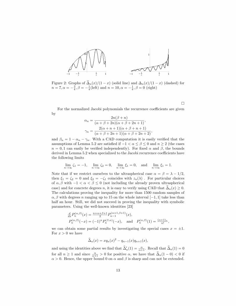
Figure 2: Graphs of ∆n(x)/(1− x) (solid line) and ∆n(x)/(1− x) (dashed) forn = 7, α = − 3

4 , β = − 14 (left) and n = 10, α = − 1

4 , β = 0 (right)

�

For the normalized Jacobi polynomials the recurrence coefficients are givenby

αn =2n(β + n)

(α+ β + 2n)(α+ β + 2n+ 1),

γn =2(α+ n+ 1)(α+ β + n+ 1)

(α+ β + 2n+ 1)(α+ β + 2n+ 2),

and βn = 1 − αn − γn. With a CAD computation it is easily verified that theassumptions of Lemma 5.2 are satisfied if −1 < α ≤ β ≤ 0 and n ≥ 2 (the casesn = 0, 1 can easily be verified independently). For fixed α and β, the boundsderived in Lemma 5.2 when specialized to the Jacobi recurrence coefficients havethe following limits

limn→∞

ζ1 = −1, limn→∞

ζ2 = 0, limn→∞

ξ1 = 0, and limn→∞

ξ1 = 1.

Note that if we restrict ourselves to the ultraspherical case α = β = λ − 1/2,then ξ1 = ζ2 = 0 and ξ2 = −ζ1 coincides with zn(λ) . For particular choicesof α, β with −1 < α < β ≤ 0 (not including the already proven ultraspherical

case) and for concrete degrees n, it is easy to verify using CAD that ∆n(x) ≥ 0.The calculations proving the inequality for more than 1500 random samples ofα, β with degrees n ranging up to 15 on the whole interval [−1, 1] take less thanhalf an hour. Still, we did not succeed in proving the inequality with symbolicparameters. Using the well-known identities [23]

ddxP

(α,β)n (x) = n+α+β+1

2 P(α+1,β+1)n−1 (x),

P (α,β)n (−x) = (−1)nP (β,α)

n (−x), and P (α,β)n (1) = (α+1)n

n! ,

we can obtain some partial results by investigating the special cases x = ±1.For x > 0 we have

∆n(x) = xqn(x)2 − qn−1(x)qn+1(x),

and using the identities above we find that ∆′n(1) = αα+1 . Recall that ∆n(1) = 0

for all n ≥ 1 and since αα+1 > 0 for positive α, we have that ∆n(1 − 0) < 0 if

α > 0. Hence, the upper bound 0 on α and β is sharp and can not be extended.

13

For x = −1 we have

∆n(−1) =

((β + 1)n(α+ 1)n

)2

− (β + 1)n−1(α+ 1)n−1

(β + 1)n+1

(α+ 1)n+1.

Using SumCracker we obtain quickly that ∆n(−1) > 0 for n ≥ 1 and α 6= β:

In[3]= ProveInequality[

((β + 1)n+1

(α+ 1)n+1

)2

−(β + 1)n

(α+ 1)n

(β + 1)n+2

(α+ 1)n+2> 0,

Using→ {−1 < α < β ≤ 0},Variable→ n]

Out[3]= TrueThe inequality above could also be easily verified by hand. Note that sinceα, β > −1 the arguments of the rising factorials are positive and so is (α +1)n+1/(β + 1)n(α+ 1)n+2/(β + 1)n+1. Multiplying the inequality by this termthe left hand side simplifies to β − α, which is positive in the given range.

In order to be able to apply a similar argument as for x = 1 we multiply∆n(x) with the factor 1 + x that is non-negative for x ∈ [−1, 0] and consider

fn(x) = (1 + x)(−xqn(x)2 − qn−1(x)qn+1(x)

)= (1 + x)∆n(x), x ∈ [−1, 0].

Now fn(−1) = 0 and fn(x) ≥ 0 if and only if ∆n(x) ≥ 0 (in [−1, 0]). Further-more, we have

f ′n(x) = ∆n(x) + (1 + x)∆′n(x),

and thus f ′n(−1) = ∆n(−1), which is positive as we showed earlier. From

these observations it follows that there exists δ > 0 such that ∆n(x) > 0 in(−1,−1 + δ) ∪ (1− δ, 1).

In conclusion we formulate a conjecture, which, if true, would yield a refine-ment of the result of Gasper [9].

Conjecture 5.3. For all n ≥ 0 and −1 < α ≤ β ≤ 0 and all x ∈ [−1, 1],

∆m(x) = |x|q2m(x)− qm−1(x)qm+1(x) ≥ 0.

References

[1] H. Alzer, S. Gerhold, M. Kauers, and A. Lupas. On Turan’s inequality forLegendre polynomials. Expo. Math., 25(2):181–186, 2007.

[2] C. Berg and R. Szwarc. Bounds on Turan determinants. J. Approx. Theory,161(1):127–141, 2009.

[3] C.W. Brown. QEPCAD B – a program for computing with semi-algebraicsets. Sigsam Bulletin, 37(4):97 – 108, 2003.

[4] C. Chen, M. Maza M. B. Xia, and L Yang. Computing cylindrical algebraicdecomposition via triangular decomposition. In ISSAC 2009—Proceedingsof the 2009 International Symposium on Symbolic and Algebraic Computa-tion, pages 95–102. ACM, New York, 2009.

14

[5] G.E. Collins. Quantifier elimination for real closed fields by cylindrical alge-braic decomposition. In Automata theory and formal languages (Second GIConf., Kaiserslautern, 1975), pages 134 – 183. Lecture Notes in Comput.Sci., Vol. 33. Springer, Berlin, 1975.

[6] D.K. Dimitrov and G.P. Nikolov. Sharp bounds for the extreme zeros ofclassical orthogonal polynomials. J. Approx. Theory, 162(10):1793–1804,2010.

[7] A. Dolzmann and T. Sturm. Redlog: computer algebra meets computerlogic. Sigsam Bulletin, 31(2):2–9, 1997.

[8] G. Gasper. On the extension of Turan’s inequality to Jacobi polynomials.Duke Math. J., 38:415–428, 1971.

[9] G. Gasper. An inequality of Turan type for Jacobi polynomials. Proc.Amer. Math. Soc., 32:435–439, 1972.

[10] S. Gerhold and M. Kauers. A Procedure for Proving Special FunctionInequalities Involving a Discrete Parameter. In Proceedings of ISSAC ’05,pages 156–162. ACM Press, 2005.

[11] S. Gerhold and M. Kauers. A computer proof of Turan’s inequality. Journalof Inequalities in Pure and Applied Mathematics, 7(2):#42, 2006.

[12] M. Kauers. SumCracker – A Package for Manipulating Symbolic Sums andRelated Objects. Journal of Symbolic Computation, 41(9):1039–1057, 2006.

[13] M. Kauers. Computer algebra and power series with positive coefficients.In Proceedings of FPSAC’07, 2007.

[14] M. Kauers. Computer algebra and special function inequalities. InTewodros Amdeberhan and Victor H. Moll, editors, Tapas in ExperimentalMathematics, volume 457 of Contemporary Mathematics, pages 215–235.AMS, 2008.

[15] M. Kauers. How To Use Cylindrical Algebraic Decomposition. SeminaireLotharingien de Combinatoire, 65(B65a):1–16, 2011.

[16] M. Kauers and P. Paule. A computer proof of Moll’s log-concavity conjec-ture. Proceedings of the AMS, 135(12):3847–3856, 2007.

[17] G. Nikolov. Inequalities of Duffin-Schaeffer type. II. East J. Approx.,11(2):147–168, 2005.

[18] V. Pillwein. Positivity of certain sums over Jacobi kernel polynomials.Advances in Applied Mathematics, 41(3):365–377, 2008.

[19] A. Seidl and T. Sturm. A generic projection operator for partial cylindricalalgebraic decomposition. In Proceedings of the 2003 International Sympo-sium on Symbolic and Algebraic Computation, pages 240 – 247 (electronic),New York, 2003. ACM.

15

[20] A. Strzebonski. Solving systems of strict polynomial inequalities. J. Sym-bolic Comput., 29(3):471 – 480, 2000.

[21] Otto Szasz. Identities and inequalities concerning orthogonal polynomialsand Bessel functions. J. Analyse Math., 1:116–134, 1951.

[22] G. Szego. On an inequality of P. Turan concerning Legendre polynomials.Bull. Amer. Math. Soc., 54:401–405, 1948.

[23] G. Szego. Orthogonal polynomials. American Mathematical Society Collo-quium Publications, Vol. 23. Revised ed. American Mathematical Society,Providence, R.I., 1959.

[24] Ryszard Szwarc. Positivity of Turan determinants for orthogonal polyno-mials. In Harmonic analysis and hypergroups (Delhi, 1995), Trends Math.,pages 165–182. Birkhauser Boston, Boston, MA, 1998.

[25] V.R. Thiruvenkatachar and T.S. Nanjundiah. Inequalities concerningBessel functions and orthogonal polynomials. Proc. Indian Acad. Sci., Sect.A., 33:373–384, 1951.

16