An analytical traffic model for the UMTS radio...
182
UNIVERSIDADE TÉCNICA DE LISBOA INSTITUTO SUPERIOR TÉCNICO Voice Shared Data C d C s C v Channels Voice analysis - P b Data analysis - L and T n v λ h v λ v λ d λ n d λ h d λ , , v v v τ μ η , , d d d τ μ η ⊕ ⊕ Buffer (B ) An analytical traffic model for the UMTS radio interface Cristina Büchel Marques dos Reis (Licenciada) Dissertation submitted for obtaining the degree of Master in Electrical and Computer Engineering Supervisor: Doctor Luís Manuel de Jesus Sousa Correia Jury: President: Doctor Luís Manuel de Jesus Sousa Correia Members: Doctor Américo Manuel Carapeto Correia Doctor José Manuel Rego Lourenço Brázio December 2003
Transcript of An analytical traffic model for the UMTS radio...
UNIVERSIDADE TÉCNICA DE LISBOA INSTITUTO SUPERIOR TÉCNICO
Voice
Shared
Data C d
C s
C v
Channels
Voice analysis- P b
Dataanalysis- L and T
nvλ
hvλ
vλ
dλndλ
hdλ
, ,v v vτ µ η
, ,d d dτ µ η⊕
⊕
Buffer (B )
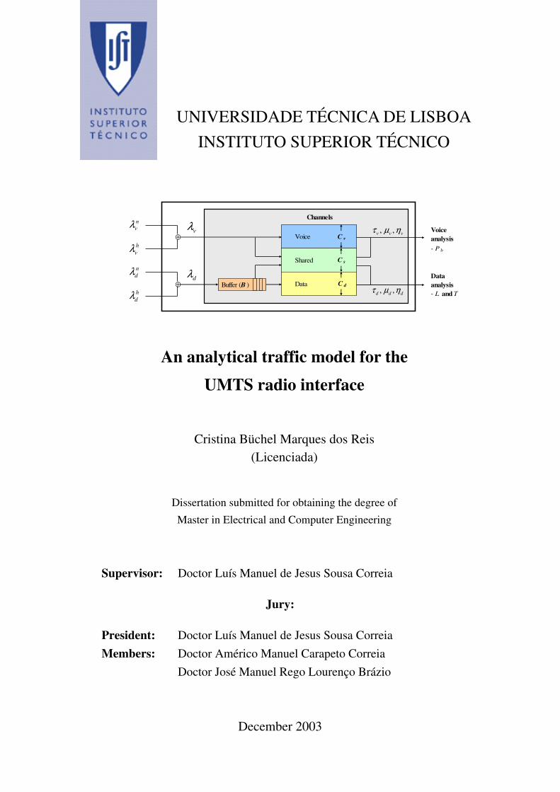
An analytical traffic model for the
UMTS radio interface
Cristina Büchel Marques dos Reis (Licenciada)
Dissertation submitted for obtaining the degree of
Master in Electrical and Computer Engineering
Supervisor: Doctor Luís Manuel de Jesus Sousa Correia
Jury:
President: Doctor Luís Manuel de Jesus Sousa Correia Members: Doctor Américo Manuel Carapeto Correia Doctor José Manuel Rego Lourenço Brázio
December 2003


To my Family

ii

iii
Acknowledgements
First of all, I wish to thank most sincerely Professor Luís Correia, for providing me with all
information and support on the elaboration of this thesis. The excellent guidelines that were
provided, sometimes even more than once a week, were determinant on the completion of this
work.
I am thankful for having been able to use the working space and facilities from Instituto de
Telecomunicações. I am also extremely grateful to have shared, for some months, the room
with a very friendly team, who, in addition, provided me with important documentation and
good tips for this work.
Special thanks are due to my Family, for their unconditional support and great incentive given
during this hard time.

iv

v
Abstract
This work is centred on the analysis of the performance of UMTS, based on the
implementation of a traffic model that integrates voice and data users, mixing circuit- and
packet-switch with a finite-buffering capacity. The model is adapted in such a way that the
main 3rd generation system characteristics are reflected in it. The generation of voice and data
events are modelled by a Poisson distribution, the service time being exponentially
distributed. Two ways of allocating channels to users are analysed: either equitably between
voice and data, or as a proportion of the number of users for each service. As expected, the
system behaves worse when the number of users or the traffic per user increases, as it imposes
a rise in the interference and a reduction on the number of channels made available by the
system. Mobility being a key issue in UMTS, its integration in the model is also accounted
for. Users’ speed is studied and the corresponding impact evaluated. Some limited
heterogeneous routing towards neighbouring cells is considered as well on the analysis of the
traffic model. The buffer size is also studied, and, as expected, it comes out that this network
element is determinant on the system performance. The analysis of a predominant voice
users’ scenario, done for a cell with 250 m radius, showed that a blocking probability of 2 %
is not exceeded for average speeds lower than 90 or 100 km/h. Considering a larger data
users’ scenario, and assuming a buffer with 15 or 20 MB, losses of 1 % become rather scarce
for any average users’ speed. In general, a reduction on the cell dimensions leads to a
remarkable improvement on the overall system performance.
Keywords
UMTS. Traffic models. Analytical model. Multi-service. System performance. Network
planning.
vi
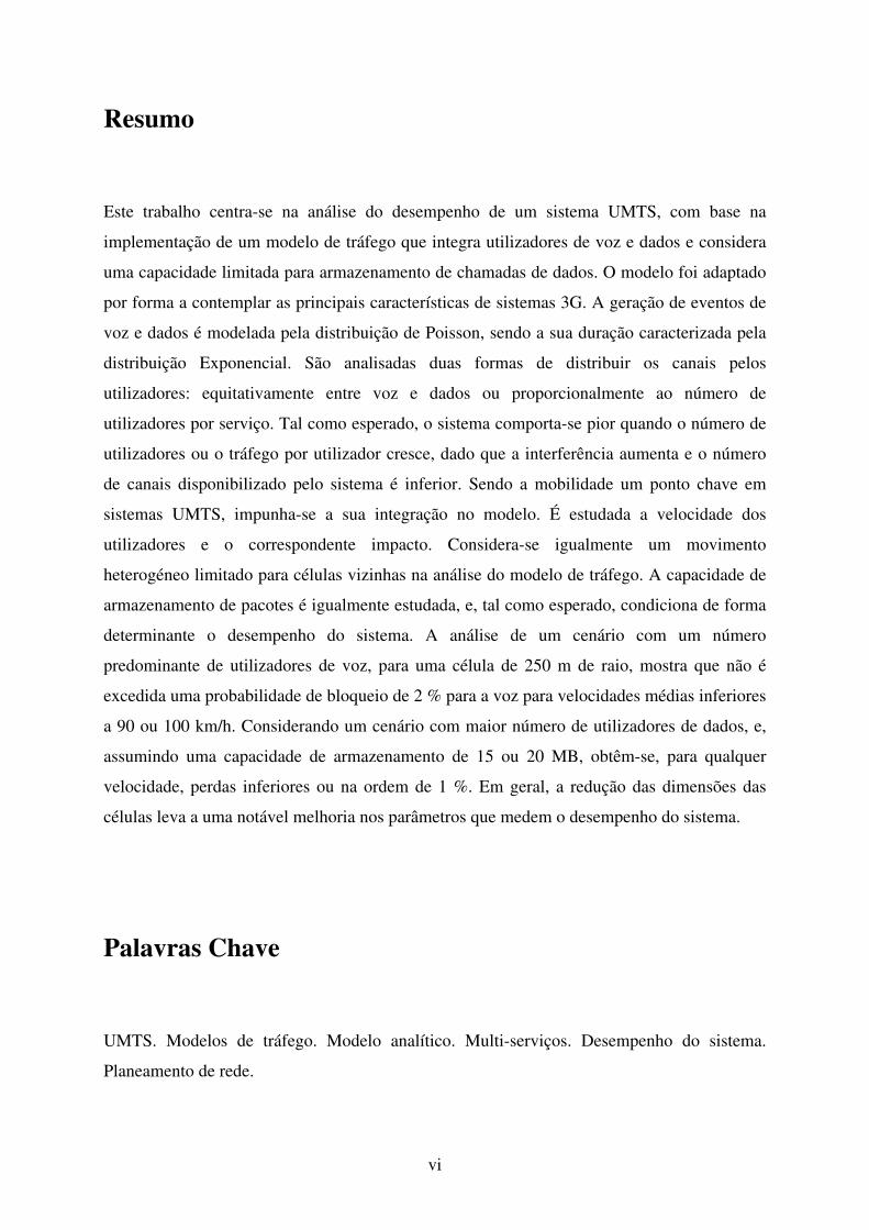
Resumo
Este trabalho centra-se na análise do desempenho de um sistema UMTS, com base na
implementação de um modelo de tráfego que integra utilizadores de voz e dados e considera
uma capacidade limitada para armazenamento de chamadas de dados. O modelo foi adaptado
por forma a contemplar as principais características de sistemas 3G. A geração de eventos de
voz e dados é modelada pela distribuição de Poisson, sendo a sua duração caracterizada pela
distribuição Exponencial. São analisadas duas formas de distribuir os canais pelos
utilizadores: equitativamente entre voz e dados ou proporcionalmente ao número de
utilizadores por serviço. Tal como esperado, o sistema comporta-se pior quando o número de
utilizadores ou o tráfego por utilizador cresce, dado que a interferência aumenta e o número
de canais disponibilizado pelo sistema é inferior. Sendo a mobilidade um ponto chave em
sistemas UMTS, impunha-se a sua integração no modelo. É estudada a velocidade dos
utilizadores e o correspondente impacto. Considera-se igualmente um movimento
heterogéneo limitado para células vizinhas na análise do modelo de tráfego. A capacidade de
armazenamento de pacotes é igualmente estudada, e, tal como esperado, condiciona de forma
determinante o desempenho do sistema. A análise de um cenário com um número
predominante de utilizadores de voz, para uma célula de 250 m de raio, mostra que não é
excedida uma probabilidade de bloqueio de 2 % para a voz para velocidades médias inferiores
a 90 ou 100 km/h. Considerando um cenário com maior número de utilizadores de dados, e,
assumindo uma capacidade de armazenamento de 15 ou 20 MB, obtêm-se, para qualquer
velocidade, perdas inferiores ou na ordem de 1 %. Em geral, a redução das dimensões das
células leva a uma notável melhoria nos parâmetros que medem o desempenho do sistema.
Palavras Chave
UMTS. Modelos de tráfego. Modelo analítico. Multi-serviços. Desempenho do sistema.
Planeamento de rede.

vii
Table of Contents
Acknowledgements..................................................................................................................iii
Abstract .....................................................................................................................................v
Keywords...................................................................................................................................v
Resumo .....................................................................................................................................vi
Palavras Chave ........................................................................................................................vi
Table of Contents....................................................................................................................vii
List of Figures ..........................................................................................................................ix
List of Tables..........................................................................................................................xiv
List of Acronyms ....................................................................................................................xv
List of Symbols.......................................................................................................................xix
1 Introduction ......................................................................................................................1
2 UMTS fundamentals ........................................................................................................9
2.1 Network architecture .............................................................................................9
2.2 Air interface.........................................................................................................11
2.3 Radio resource management ...............................................................................15
2.4 Services and applications ....................................................................................17
2.5 Network dimensioning ........................................................................................18
3 Traffic analysis ...............................................................................................................25
3.1 Coverage estimation ............................................................................................25
3.2 Capacity estimation .............................................................................................32

Table of Contents
viii
3.3 Code planning......................................................................................................37
3.4 General traffic aspects .........................................................................................41
4 Traffic model...................................................................................................................49
4.1 Model formulation...............................................................................................49
4.2 Adaptation of the model to UMTS......................................................................53
4.3 The algorithm ......................................................................................................65
5 Analysis of results...........................................................................................................75
5.1 Description of scenarios under study ..................................................................75
5.2 Analysis of the number of channels ....................................................................79
5.3 Comparison of traffic model results with known models ...................................81
5.4 Results for a single cell .......................................................................................87
5.5 Results for multi-cells .........................................................................................98
6 Conclusions ...................................................................................................................103
Annex A COST231–Walfisch-Ikegami Model..............................................................109
Annex B Statistical distributions ...................................................................................113
Annex C Scenario A, Program results...........................................................................115
Annex D Scenario B, Program results...........................................................................133
References ...........................................................................................................................151

ix
List of Figures
Figure 1.1 – International allocations for IMT-2000 (extracted from [CEPT00]). ....................1
Figure 1.2 – Third generation environment (adapted from [CEPT00]). ....................................3
Figure 2.1 – General UMTS network architecture (adapted from [3GPP01a]). ........................9
Figure 2.2 – UMTS Spectrum allocations in Europe (based on [CEPT02]). ...........................12
Figure 2.3 – Example of services and applications in UMTS (adapted from [UMTS01]). .....18
Figure 3.1 – Cell radius. ...........................................................................................................31
Figure 3.2 – Coverage vs. capacity on UL and DL. .................................................................36
Figure 3.3 – Code-tree for generation of OVSF codes (extracted from [3GPP01b])...............37
Figure 3.4 – Maximum number of DL users per service (based on [FCSC02]). .....................40
Figure 3.5 – Maximum number of users for more than one service. .......................................40
Figure 3.6 – General call access mechanism for CS (extracted from [Corr03]). .....................44
Figure 3.7 – General call access mechanism for PS (adapted from [Leon94]). .......................46
Figure 4.1 – Traffic model for the base station (adapted from [HaLH00])..............................49
Figure 4.2 – DL Code check. ...................................................................................................54
Figure 4.3 – Eb/N0 values (adapted from [RFHL03])...............................................................55
Figure 4.4 – Orthogonal factor as a function of users’ speed...................................................56
Figure 4.5 – Link budget parameters adapted to a varying users’ speed. ................................57
Figure 4.6 – Call arrival rate vs. cell radius. ............................................................................60
Figure 4.7 – pij matrix...............................................................................................................61
Figure 4.8 – Steady-states [(τv, τd), (λv, λd)].............................................................................62
Figure 4.9 – Steady-states [(2τv, 2τd), (λv, λd)] or [(τv, τd), (2λv, 2λd)]. ...................................62
Figure 4.10 – Users’ motion along a ring of six cells. .............................................................65

List of Figures
x
Figure 4.11 – Channel distribution...........................................................................................68
Figure 4.12 – Traffic model algorithm, main flowchart...........................................................70
Figure 4.13 – System load verification, flowchart A. ..............................................................71
Figure 4.14 – Code verification, flowchart B...........................................................................72
Figure 4.15 – BS power verification, flowchart C. ..................................................................73
Figure 4.16 – Traffic model computation, flowchart D. ..........................................................74
Figure 5.1 – Possible cell radii. ................................................................................................78
Figure 5.2 – Number of codes for Scenario A. ........................................................................79
Figure 5.3 – Number of codes for Scenario B..........................................................................80
Figure 5.4 – Blocking probability for Erlang-B model. ...........................................................82
Figure 5.5 – Available voice channels versus users’ speed......................................................83
Figure 5.6 – Traffic model blocking probability for Scenario B..............................................84
Figure 5.7 – Erlang-B model blocking probability, Scenario A...............................................85
Figure 5.8 – Erlang-B model blocking probability, Scenario B...............................................86
Figure 5.9 – Equitable distribution of channels. ......................................................................88
Figure 5.10 – Proportional distribution of channels, predominant voice users........................89
Figure 5.11 – Proportional distribution of channels, predominant data users..........................90
Figure 5.12 – Blocking probability as a function of users’ speed. ...........................................92
Figure 5.13 – Data loss probability as a function of users’ speed............................................93
Figure 5.14 – Mean data delay as a function of users’ speed...................................................94
Figure 5.15 – Pb and L as a function of the users’ speed, for R = 100 m. ................................95
Figure 5.16 – Pb and L as a function of the users’ speed, for R = 200 m. ................................96
Figure 5.17 – Mean data delay vs. speed for a heterogeneous scenario.................................100
Figure 5.18 – Mean data delay per cell for a heterogeneous scenario. ..................................101

List of Figures
xi
Figure A.1 – Parameters used in the COST231-Walfisch-Ikegami model (extracted from
[Corr99]). ..........................................................................................................109
Figure B.1 – Discrete distribution of events (extracted from [Keis89]).................................113
Figure C.1 – Number of codes for Scenario A with a 150 and 250 m cell radius..................115
Figure C.2 – System performance versus users’ speed (150 m cell radius; 20 MB buffer
size)...................................................................................................................116
Figure C.3 – System performance versus users’ speed (250 m cell radius; 20 MB buffer
size)...................................................................................................................117
Figure C.4 – System performance versus users’ speed (150 m cell radius; 10 MB buffer
size)...................................................................................................................118
Figure C.5 – System performance versus users’ speed (250 m cell radius; 10 MB buffer
size)...................................................................................................................119
Figure C.6 – System performance versus buffer size (150 m cell radius; 15 km/h average
speed)................................................................................................................120
Figure C.7 – System performance versus buffer size (250 m cell radius; 15 km/h average
speed)................................................................................................................121
Figure C.8 – System performance versus buffer size (150 m cell radius; 60 km/h average
speed)................................................................................................................122
Figure C.9 – System performance versus buffer size (250 m cell radius; 60 km/h average
speed)................................................................................................................123
Figure C.10 – Steady-states [(τv, τd), (λv, λd)], equitable distribution of resources and
150 m cell radius...............................................................................................124
Figure C.11 – Steady-states [(2τv, 2τd), (λv, λd)] or [(τv, τd), (2λv, 2λd)], equitable
distribution of resources and 150 m cell radius. ...............................................125
Figure C.12 – Steady-states [(τv, τd), (λv, λd)], proportional distribution of resources and
150 m cell radius...............................................................................................126
Figure C.13 – Steady-states [(2τv, 2τd), (λv, λd)] or [(τv, τd), (2λv, 2λd)], proportional
distribution of resources and 150 m cell radius. ...............................................127
List of Figures
xii
Figure C.14 – Steady-states [(τv, τd), (λv, λd)], equitable distribution of resources and
250 m cell radius...............................................................................................128
Figure C.15 – Steady-states [(2τv, 2τd), (λv, λd)] or [(τv, τd), (2λv, 2λd)], equitable
distribution of resources and 250 m cell radius. ...............................................129
Figure C.16 – Steady-states [(τv, τd), (λv, λd)], proportional distribution of resources and
250 m cell radius...............................................................................................130
Figure C.17 – Steady-states [(2τv, 2τd), (λv, λd)] or [(τv, τd), (2λv, 2λd)], proportional
distribution of resources and 250 m cell radius. ...............................................131
Figure D.1 – Number of channels for Scenario B. .................................................................133
Figure D.2 – System performance versus users’ speed (150 m cell radius; 20 MB buffer
size)...................................................................................................................134
Figure D.3 – System performance versus users’ speed (250 m cell radius; 20 MB buffer
size)...................................................................................................................135
Figure D.4 – System performance versus users’ speed (150 m cell radius; 10 MB buffer
size)...................................................................................................................136
Figure D.5 – System performance versus users’ speed (250 m cell radius; 10 MB buffer
size)...................................................................................................................137
Figure D.6 – System performance versus buffer size (150 m cell radius; 15 km/h average
speed)................................................................................................................138
Figure D.7 – System performance versus buffer size (250 m cell radius; 15 km/h average
speed)................................................................................................................139
Figure D.8 – System performance versus buffer size (150 m cell radius; 60 km/h average
speed)................................................................................................................140
Figure D.9 – System performance versus buffer size (250 m cell radius; 60 km/h average
speed)................................................................................................................141
Figure D.10 – Steady-states [(τv, τd), (λv, λd)], equitable distribution of resources and
150 m cell radius...............................................................................................142
List of Figures
xiii
Figure D.11 – Steady-states [(2τv, 2τd), (λv, λd)] or [(τv, τd), (2λv, 2λd)], equitable
distribution of resources and 150 m cell radius. ...............................................143
Figure D.12 – Steady-states [(τv, τd), (λv, λd)], proportional distribution of resources and
150 m cell radius...............................................................................................144
Figure D.13 – Steady-states [(2τv, 2τd), (λv, λd)] or [(τv, τd), (2λv, 2λd)], proportional
distribution of resources and 150 m cell radius. ...............................................145
Figure D.14 – Steady-states [(τv, τd), (λv, λd)], equitable distribution of resources and
250 m cell radius...............................................................................................146
Figure D.15 – Steady-states [(2τv, 2τd), (λv, λd)] or [(τv, τd), (2λv, 2λd)], equitable
distribution of resources and 250 m cell radius. ...............................................147
Figure D.16 – Steady-states [(τv, τd), (λv, λd)], proportional distribution of resources and
250 m cell radius...............................................................................................148
Figure D.17 – Steady-states [(2τv, 2τd), (λv, λd)] or [(τv, τd), (2λv, 2λd)], proportional
distribution of resources and 250 m cell radius. ...............................................149
xiv
List of Tables
Table 2.1 – Main characteristics of channelisation and scrambling codes (based on
[HoTo01]). ..........................................................................................................14
Table 2.2 – UMTS traffic classes (extracted from [3GPP02a]). ..............................................19
Table 2.3 – Radio bearer attributes per UMTS QoS class (as defined in [3GPP02a]).............20
Table 3.1 – MTs and BSs assumptions (based on [HoTo01])..................................................27
Table 3.2 – Eb/N0 used for link budget calculations (extracted from [FCSC02]). ...................28
Table 3.3 – Services vs. UL/DL spreading factors and UL/DL codes (adapted from
[FCSC02]). .........................................................................................................39
Table 4.1 – Lin-car , GSHO and Mfast-fading vs. number of channels. .............................................58
Table 5.1 – Number of users forming Scenarios A and B........................................................75
Table 5.2 – Services characteristics (adapted from [FCXV03]). .............................................76
Table 5.3 – Input parameters common to Scenarios A and B. .................................................77
Table 5.4 – No. of codes for R = 200 m at 30 km/h, Scenarios A and B. ................................77
Table 5.5 – System tendency due to the traffic model. ............................................................98
xv
List of Acronyms
2.5G Interim step towards 3rd Generation of mobile system
2G 2nd Generation of mobile systems
3G 3rd Generation of mobile systems
3GPP 3rd Generation Partnership Project
AICH Acquisition Indication Channel
BCCH Broadcast Control Channel
BCH Broadcast Channel
BHCA Busy Hour Call Attempt
BS Base Station
BSC Base Station Controller
BSS Base Station Subsystem
CCCH Common Control Channel
CCPCH Common Control Physical Channel
CDMA Code Division Multiple Access
CN Core Network
CPCH Common Packet Channel
CPICH Common Pilot Channel
CS Circuit Switched
CTCH Common Traffic Channel
DCCH Dedicated Control Channel
DCH Dedicated Channel

List of Acronyms
xvi
DL Downlink
DPCCH Dedicated Physical Control Channel
DPCH Dedicated Physical Channel
DPDCH Dedicated Physical Data Channel
DS-CDMA Direct Sequence Code Division Multiple Access
DSCH Downlink Shared Channel
DTCH Dedicated Traffic Channel
EDGE Enhanced Data for Global Evolution
EIRP Equivalent Isotropic Radiated Power
E-Mail Electronic Mail
ETSI European Telecommunications Standards Institute
FACH Forward Access Channel
FCFS First-Come-First-Served
FDD Frequency Division Duplex
FDMA Frequency Division Multiple Access
FDwnld File Download
FTP File Transfer Protocol
GPRS General Packet Radio Service
GSM Global System for Mobile communications
HLR Home Location Register
HO Handover
HSCSD High Speed Circuit Switched Data
iid Independent and identically distributed
IP Internet Protocol

List of Acronyms
xvii
ITU-T International Telecommunications Union, Telecommunications Sector
LocBas Location Based
MAC Medium Access Control
MMS Multimedia Messaging Service
MSS Mobile Satellite Service
MT Mobile Terminal
NSS Network Subsystem
OSI Open Systems Interconnection
OVSF Orthogonal Variable Spreading Factor
PCCH Paging Control Channel
P-CCPCH Primary Common Control Physical Channel
PCH Paging Channel
PCPCH Physical Common Packet Channel
PDSCH Physical Downlink Shared Channel
PHY Physical Layer
PICH Page Indication Channel
PN Pseudo Noise
PRACH Physical Random Access Channel
PS Packet Switched
QoS Quality of Service
RAB Radio Access Bearer
RACH Random Access Channel
RLC Radio Link Control
RNC Radio Network Controller
List of Acronyms
xviii
RNS Radio Network Subsystems
RRM Radio Resource Management
S-CCPCH Secondary Common Control Physical Channel
SCH Synchronisation Channel
SF Spreading Factor
SIR Signal to Interference Ratio
SMS Short Message Service
SNR Signal-to-Noise Ratio
Speech Speech-Telephony
StrMMHQ Streaming Multimedia High Quality
StrMMLQ Streaming Multimedia Low Quality
TDD Time Division Duplex
TDMA Time Division Multiple Access
UE User Equipment
UL Uplink
UMTS Universal Mobile Telecommunications System
USCH Uplink Shared Channel
USIM UMTS Subscriber Identity Module
UTRAN UMTS Terrestrial Radio Access Network
VideoT Video-Telephony
WCDMA Wideband Code Division Multiple Access
WWW Web Browsing

xix
List of Symbols
α Angle between horizon (at hb-HB) and hb, seen by building diffraction point
α Average orthogonality factor in the cell
φ Road orientation with respect to the direct radio path
η Cell load
ηd Cell cross-over rate for data users
ηDL DL load factor
ηh Cell cross-over rate
ηUL UL load factor
ηv Cell cross-over rate for voice users
λ Arrival rate
λd Data call rate
λd100 Data call rate for a 100 m cell radius
λdh HO data call rate
λdn New data call rate
λh HO call arrival rate
λn New call arrival rate
λv Voice call rate
λv100 Voice call rate for a 100 m cell radius
λvh HO voice call rate
λvn New voice call rate

List of Symbols
xx
µcd Data channel occupancy rate
µcv Voice channel occupancy rate
µd Data call service rate
µv Voice call service rate
ρ Utilisation of a system
στ Standard deviation of τ
τ Average call duration
τc Channel occupancy time in the cell
τd Data call duration
τh Average dwell time in a cell
τv Voice call duration
�j Activity factor of user j at physical level
ξh HO rate
A Amount of traffic
B Buffer size
c Number of servers (channels)
C Number of channels
Cτ2 Coefficient of variation of the service time
Cd Number of data channels
Cg Number of channels for new generated calls
Ch Number of channels for HO calls
Cs Number of shared channels
Cv Number of voice channels
d Distance

List of Symbols
xxi
Eb Energy per user bit
f Frequency
FN Noise figure
Gdiv Diversity gain
Gr Antenna gain at the reception
GSHO Soft handover gain
Gt Antenna gain at the transmission
hb BS height
HB Heights of buildings
hm MT height
Hroof Roof height
i Other cell to own interference ratio seen by the BS
ka BS height correction factor
kd Distance correction factor
kf Frequency correction factor
L Data loss probability
L0 Free space loss
Lbsh Loss due to BS height
Lbuilding Building penetration loss
Lc Cable losses at the BS
Lin-car In-car loss
Lmsd Multi-screen loss
Lori Loss due to orientation
Lp Allowed propagation loss

List of Symbols
xxii
Lrts Roof-top-to-street diffraction and scatter loss
Mbody-loss Body loss margin
Mfast-fading Fast fading margin
Mint Interference margin
Mlog-normal Log-normal fading margin
N Number of users per cell
N0 Noise power
DLnpoleN DL pole capacity for the nth RAB
ULnpoleN UL pole capacity for the nth RAB
Nrf Noise spectral density of the MT receiver front-end
p0 Probability at state 0
Pb Probability of blocking calls
pc Probability at state c
Pd Drop call probability
pd(j) Probability of having j data packet transmissions
Ph Probability of performing HO
Phf Probability of HO failure
Pii Probability generating function
pij Steady-state probability of i voice calls and j data packets
Pr Power at the reception
Pr min Receiver sensitivity
Pt Power at the transmission
PTxBS BS transmitted power

List of Symbols
xxiii
pv(i) Probability of having i voice calls
Pw Probability that a call waits in a queue
qij Tail probability of j data packets when there are i voice calls
R Cell radius
Rb Service bit rate
Rb j Service bit rate of user j
Rc WCDMA chip rate
rij Routing probability from cell i to cell j
Rij Routing matrix
Rn Service bit rate of the nth RAB
T Mean data delay
v Mean velocity
wB Building separation
WB Widths of roads considering building walls
ws Widths of roads
z Complex number

xxiv
1
1 Introduction
A long way has been left behind since it was first heard about the 3rd generation of mobile
systems (3G), namely IMT-2000 or even UMTS. Many thoughts were discussed within the
standardisation bodies, leading to the presentation of a variety of multiple radio access
techniques and several standards. Originally, and in a wide sense, 3G aimed at:
- converging to a common world standard;
- allowing both voice and high speed data;
- using in a more efficient way the available spectrum;
- simplifying international roaming;
- attaining economies of scale in equipment production.
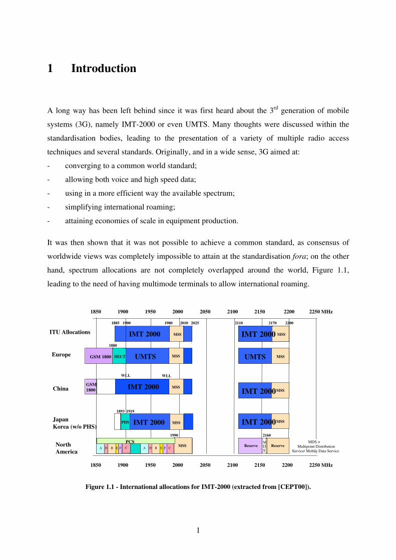
It was then shown that it was not possible to achieve a common standard, as consensus of
worldwide views was completely impossible to attain at the standardisation fora; on the other
hand, spectrum allocations are not completely overlapped around the world, Figure 1.1,
leading to the need of having multimode terminals to allow international roaming.
Figure 1.1 - International allocations for IMT-2000 (extracted from [CEPT00]).
1850 1900 1950 2000 2050 2100 2150 2200 2250 MHz
1850 1900 1950 2000 2050 2100 2150 2200 2250 MHz
NorthAmerica
MSS Reserve
Europe UMTSGSM 1800 DECT MSS
1880
1980
JapanKorea (w/o PHS)
MSSIMT 2000PHS MSSIMT 20002160
1893 1919
ITU Allocations1885
IMT 2000
2010 2110 2170
China MSSIMT 2000IMT 2000
IMT 2000
MSSUMTS
MSS
1990
A D B E F A B C ReserveMDS
WLL WLL
2025 22001900 MSS MSS
GSM1800
D FE B B
PCS C
MDS = Multipoint Distribution
Service/ Mobile Data Service

1. Introduction
2
3G will extensively introduce the Wideband Code Division Multiple Access (WCDMA)
approach. Despite of the huge investment already done in 2nd generation (2G) Time Division
Multiple Access (TDMA) systems in Europe and in other parts of the world, e.g., Global
System for Mobile communications (GSM), this new access method was the one approved for
UMTS. Operators that work with TDMA systems need to change a considerable amount of
network elements in order to get on track with CDMA.
An intermediate step between 2G and 3G, namely the 2.5G (interim step towards 3rd
Generation, based on upgrading the GSM network to provide data services faster than 2G
GSM), was envisaged to fit in the timeframe within which 3G was still under development,
and where 2G could no longer satisfy the users requirements and needs. High Speed Circuit
Switched Data (HSCSD), with up to 57.6 kbps by using several traffic channels, General
Packet Radio Service (GPRS), with up to 115 kbps by using additional network elements that
allow the Mobile Terminal (MT) to form a packet switched connection through the GSM
network to an external packet data network, or even the Enhanced Data for Global Evolution
(EDGE), with up to 384 kbps by implementing a new air interface modulation (8-PSK) and
sophisticated channel coding techniques, were the strongest proposed predecessors for 3G
systems.
UMTS data rates, as promised, would make it possible to offer all kinds of new services to 3G
users. The most common examples of service are [FCSC02]:
- Speech- and Video-telephony;
- Streaming multimedia;
- Web browsing;
- Location based;
- Short message service (SMS) and Multimedia messaging service (MMS);
- E-Mail;
- File download.
The majority of users will certainly keep, for a rather long time, voice as one of the most
requested services. Short messages, as used in 2G, especially by youth, which corresponds to
the first data service possible through an MT, will probably tend to disappear in the
meantime, as the awakening of multimedia messages seem to attract a lot of people. Internet

1. Introduction
3
access, from everywhere, at any time and at a reasonable price, is one of the most interesting
promises that are being announced by many 3G operators; interactivity on the mobile phones
is, as well, a wish for many persons. These tempting examples and users’ expectations do not
summarise the wish list of the majority of people; there are many other services and
applications, some even still being studied, which will certainly be disclosed as soon as the
commercial use of 3G networks is launched.
UMTS was, from the start, conceived to be a global system, comprising national terrestrial
and satellite components, while 2G systems are expected to be used to extend coverage for
less demanding services. Roaming from a private cordless or fixed network into a pico- or
micro-cellular public network, and then into a wide area macro-cellular network, and, if
necessary, into a satellite mobile one, and, in each case, with a minimal break in
communication, seems to be the greatest challenge for the current 3G drivers. Contemporary
mobile users live in a multi-dimensional world, moving between indoor, outdoor urban and
outdoor rural environments, with a degree of mobility ranging from essentially stationary
through pedestrian, up to very high vehicular speeds, as shown in Figure 1.2.
Figure 1.2 – Third generation environment (adapted from [CEPT00]).
This seems to be achievable if boundaries between networks, operators and countries are
blurred. Great cooperation is thus required in the future, to enable not only international

1. Introduction
4
roaming to the demanding 3G users, but also seamless roaming on a national basis, to allow
access to diverse environments and/or miscellaneous networks, ruled by distinct technologies,
and which will not disappear in the coming years or decades, due to the fact that they
complement each other.
After knowing which services may be used by future UMTS subscribers, it becomes
important to understand their spatial and temporal incidence; along the day, as well as during
a week period, some typical usage behaviours are important to be depicted, as they will
absolutely determine the overall system capacity. To characterise the diversity of service
usage patterns that UMTS can sustain, it is worthwhile to distinguish between three customer
segments [FCSC02]:
• Business, with intensive and almost entirely professional use, primarily during working
hours;
• Small Office Home Office (SOHO), with both professional and private use, during the
day and in the evening;
• Mass-market, with low use, staying within flat traffic levels.
Users of distinct customer segments are spread differently over the operational environment,
according to their specific characteristics; the amount of calls generated per service may, thus,
assume different values per customer segment.
It is known that there is currently very little information, besides marketing estimates, on the
amount of traffic that UMTS networks are expected to cope with. It is also difficult to find
any information on models that show adequately the behaviour of UMTS users and
consequences in terms of system performance, allowing multi-service traffic to be estimated.
Due to the scarce information and experience with 3G systems, it is of great interest to predict
the amount of traffic generated by all kinds of users, so that the performance of UMTS
networks is studied and a better dimensioning of the systems is carried out. Although voice in
3G may have some similarities with 2G, and the well-known traffic models could still be
appropriate if adapted (e.g., the Erlang-B model), the same does not apply for data services
over the CDMA technology that is behind the new mobile network’s generation, where so
many parameters influence the overall system performance and an extensive analysis of the
subject is required, before the first accurate results are available.

1. Introduction
5
The idea of studying traffic matters for UMTS is a popular one these days, in view of finding
and investigating a model that could deal with both voice and data services; UMTS reality
implies that many new aspects, not considered as 2G systems’ key issues, are as well
accounted for during the planning of activities for 3G, e.g., asymmetric bandwidth
requirements and code planning needs.
Several research projects and groups already tackled this very challenging subject, providing
some valuable contributions in this area. The IST-MOMENTUM European project
[MOME01], for example, developed a considerable amount of work and documentation on
the analysis of UMTS system-behaviour and the optimisation of radio network design,
through the deployment of new planning methods, with support of system manufacturers,
network operators, service providers and university research teams. Additionally, [CaVa02]
provided traffic modelling for UMTS, basing many assumptions on criteria resulting from
Population and Housing Census in Portugal, performed in 2001, and topographic
information. Moreover, [Serr02] resulted in a valuable contribution on optimisation of cell
radius in UMTS-FDD networks, presenting a new tool that was developed to perform many
system calculations, converting its output in the optimum cell radius for a given scenario.
More recently, [Dias03] further improved the work presented in [Serr02], by complementing
it with specific traffic source models for each service, combining, for various scenarios,
different services with distinct call rates and penetration factors, and analysing, as a
consequence, the overall system performance. Last, but not least, [HaLH00] proposed an
analytical model to investigate the performance of an integrated voice/data mobile network
with finite data buffer, which served as a starting point for the current work.
This thesis deals with an analytical traffic model that integrates voice and data services,
mixing circuit- and packet-switch, and considering a finite data-buffering capacity. The model
is adapted to reflect 3G system characteristics, a detailed study from the system performance
perspective being presented. Parameters like users’ speed, cell radii, call characteristics (rates
and average duration) and capacity to store data, are analysed. To accomplish this ambitious
task, some approximations are made, in order to avoid an extreme complexity of the model,
allowing it to be practical and functional.

1. Introduction
6
It is worthwhile saying that the present work will exclusively be focused on the UMTS
Frequency Division Duplex (FDD) mode of operation; the standardisation of the Time
Division Duplex (TDD) mode is still not completely finished by the corresponding entities.
Nevertheless, it is of great importance to consider, as soon as there is any supporting
documentation, this mode of operation, as it may improve considerably the efficient use of
resources in UMTS, especially for asymmetric services.
The current analytical model introduces an innovative approach when performing the
integration of distinct services, voice and data, commonly supported by networks with
separate structures, circuit- and packet-switched, allowing, through a single model, the
estimation of the traffic amount generated by a UMTS network and its corresponding system
performance. The scenarios in terms of number of users per service may be varied; the main
system parameters (e.g., call rates, system load, Base Station (BS) power, types of services
and corresponding duration) may as well be modified, allowing the model to suit the purposes
of the environment particularities and specific UMTS users’ characteristics.
The present work is composed of six chapters, including the current one; in addition, four
Annexes are appended to this document. In Chapter 2, a brief overview of essential UMTS
fundamentals is presented. Chapter 3 provides a general description covering the main
particular UMTS aspects that need to be reflected in the traffic model analysis; more
specifically, the major coverage, capacity and code planning guidelines are depicted, as well
as the most important traffic aspects that are required for the subsequent work. Chapter 4 is
devoted to the analytical traffic model; first of all, its formulation is presented in detail;
afterwards, all aspects where a model adaptation is required are described; at the end of the
chapter, the algorithm as implemented is explained, with the aid of the corresponding detailed
flowcharts. In Chapter 5, the output of the analytical traffic model is extensively analysed: the
scenarios under study are described, an explanation on the variable channel number is
provided, and a comparison of the output of the model with that of other traffic models is
performed; finally, the results of the traffic model applied to a single cell are analysed; a
multi-cell scenario, where users’ movement is not homogeneous, is summarised as well and
the motion repercussions depicted. Chapter 6 presents the final conclusions and further
suggestions of work to be done in the future. Finally, Annex A contains the formulation of the
COST231-Walfisch-Ikegami propagation model, required for the estimation of the cell radius;

1. Introduction
7
Annex B comprises the statistical distributions referred along the thesis; Annexes C and D
contain the complete set of results for the two scenarios under study.

8

9
2 UMTS fundamentals
2.1 Network architecture
UMTS is divided into Core Network (CN), UMTS Terrestrial Radio Access Network
(UTRAN) and User Equipment (UE), [3GPP01a], Figure 2.1.
Figure 2.1 – General UMTS network architecture (adapted from [3GPP01a]).
The UMTS architecture was designed in such a way that the CN can be connected to a variety
of UTRAN subsystems, which is a step forward when compared to 2G; it is known that GSM
operators that had on their network Base Station Subsystems (BSSs) and Network Subsystems
(NSSs) from different vendors experienced considerable problems of interoperability. The Iu
interface in UMTS was conceived to be an open one, meaning that, in theory at least, different
vendors’ equipment could be put together, if they fulfilled the standards. This allows the
coexistence of different standards, not only 3G, but also the enhanced 2G technologies, and a
cost efficient deployment, maximising the use of the GSM/GPRS infrastructure, as well as the
implementation of Internet Protocol (IP) technologies.

2. UMTS fundamentals
10
The UMTS CN consists of two specific domains, the circuit (CS) and the packet (PS)
switched ones, the latter being the major novelty introduced by UMTS when compared with
2G systems, which were clearly CS oriented at the beginning. The separation between the CS
and PS domains inside the CN allows a simpler evolution from GSM/GPRS, with lower risks,
an earlier availability and service continuity. On the other hand, operators need to build and
manage two different networks, perform separate engineering and dimensioning, and invest
on two distinct infrastructures. CN functions may be summarised as follows:
- Switching;
- Service availability;
- Transmission of user traffic between UTRAN(s) and/or fixed network(s);
- Mobility management;
- Operations, Administration and Maintenance.
The UTRAN consists of one or several Radio Network Subsystems (RNSs) connected to the
CN through the Iu interface. Each RNS contains one Radio Network Controller (RNC) and
one or several Node Bs. The RNC owns and controls the radio resources in its domain, and
acts as the service access point for all services that UTRAN provides to the CN; the Node B
corresponds to the radio BS and converts the data flow between the Iub and the Uu interfaces.
The major difference in the radio access network between GSM and UMTS corresponds to
the fact that in UMTS, the RNC (the counterpart of the Base Station Controller (BSC) in
GSM) is partly in charge of the mobility management, whereas the BSC is not responsible for
this function. UTRAN functions may be summarised as follows:
- Provision of radio coverage;
- System access control;
- Security and privacy;
- Handover;
- Radio resource management and control.
The UE consists of two parts: the MT, which corresponds to the radio terminal used for radio
communication over the Uu air interface, and the UMTS Subscriber Identity Module (USIM),
the GSM equivalent smart card, that holds the subscriber identity, performs authentication
algorithms, stores authentication and encryption keys, etc. There are no major differences
between the 2G and 3G MTs, except for the fact that 3G terminals are expected to have a
2. UMTS fundamentals
11
completely new layout, with a tempting and attractive monitor to encourage data calls. UE
functions may be summarised as follows:
- Display of the user interface;
- Holding of the authentication algorithms and keys;
- User and termination of the air interface;
- Application platform.
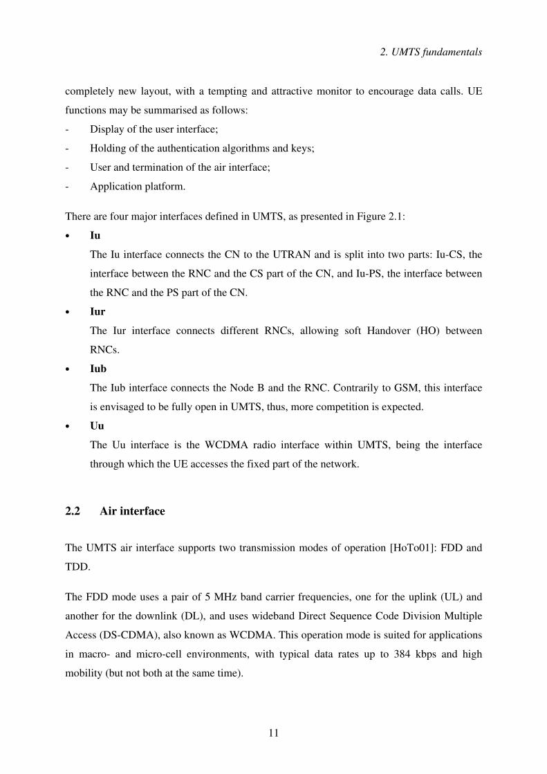
There are four major interfaces defined in UMTS, as presented in Figure 2.1:
• Iu
The Iu interface connects the CN to the UTRAN and is split into two parts: Iu-CS, the
interface between the RNC and the CS part of the CN, and Iu-PS, the interface between
the RNC and the PS part of the CN.
• Iur
The Iur interface connects different RNCs, allowing soft Handover (HO) between
RNCs.
• Iub
The Iub interface connects the Node B and the RNC. Contrarily to GSM, this interface
is envisaged to be fully open in UMTS, thus, more competition is expected.
• Uu
The Uu interface is the WCDMA radio interface within UMTS, being the interface
through which the UE accesses the fixed part of the network.
2.2 Air interface
The UMTS air interface supports two transmission modes of operation [HoTo01]: FDD and
TDD.
The FDD mode uses a pair of 5 MHz band carrier frequencies, one for the uplink (UL) and
another for the downlink (DL), and uses wideband Direct Sequence Code Division Multiple
Access (DS-CDMA), also known as WCDMA. This operation mode is suited for applications
in macro- and micro-cell environments, with typical data rates up to 384 kbps and high
mobility (but not both at the same time).

2. UMTS fundamentals
12
The TDD mode uses a single 5 MHz band carrier frequency, shared between the up- and the
downlink connections, being the result of the combination of TDMA and CDMA, and
exploiting spreading as part of its CDMA component. This mode of operation is advantageous
for public micro- and pico-cell environments, since it facilitates the efficient use of the
unpaired spectrum and supports data rates up to 2 Mbps. Therefore, the TDD mode is suited
for environments with high traffic densities and indoor coverage, where applications require
high data rates and tend to create asymmetric traffic.
The combined deployment of the FDD and TDD modes will enable a more efficient use of the
available spectrum, by considering the advantages and avoiding the disadvantages of each of
these modes. Nevertheless, there are still some ongoing standardisation activities for
definition of the UMTS TDD mode. It is expected that the first TDD networks will appear
some two years after the FDD mode is put into operation.
As shown in Figure 2.2, the amount of spectrum allocated in Europe to the FDD and TDD
modes, as well as to its satellite component, corresponds to:
- 2 × 60 MHz of paired spectrum for use in FDD mode;
- 35 MHz of unpaired spectrum for use in TDD mode;
- 2 × 30 MHz for use in the satellite component.
Figure 2.2 – UMTS spectrum allocations in Europe (based on [CEPT02]).
In Portugal, the terrestrial component of the available spectrum for UMTS is split among
three operators that were awarded a 3G license. Each of the operators owns, for the 15-year
period of duration of its license, 2 × 20 MHz of paired spectrum (FDD) and one additional
carrier frequency, 5 MHz, of unpaired spectrum (TDD).
2. UMTS fundamentals
13
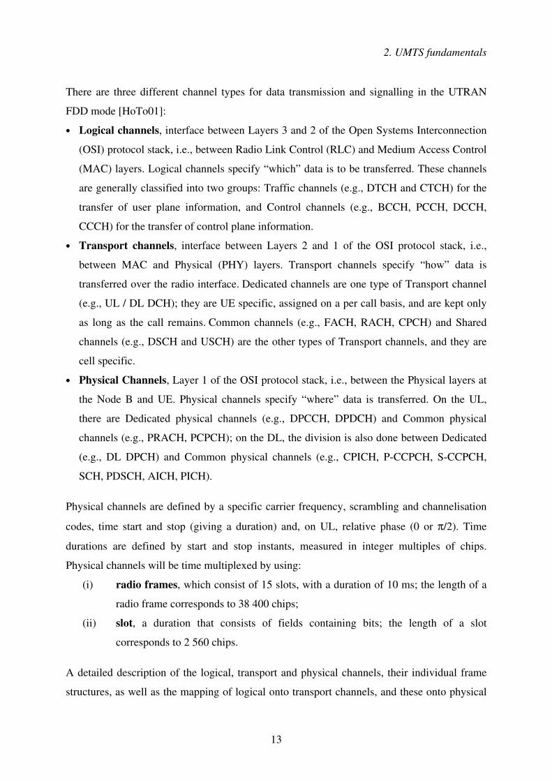
There are three different channel types for data transmission and signalling in the UTRAN
FDD mode [HoTo01]:
• Logical channels, interface between Layers 3 and 2 of the Open Systems Interconnection
(OSI) protocol stack, i.e., between Radio Link Control (RLC) and Medium Access Control
(MAC) layers. Logical channels specify “which” data is to be transferred. These channels
are generally classified into two groups: Traffic channels (e.g., DTCH and CTCH) for the
transfer of user plane information, and Control channels (e.g., BCCH, PCCH, DCCH,
CCCH) for the transfer of control plane information.
• Transport channels, interface between Layers 2 and 1 of the OSI protocol stack, i.e.,
between MAC and Physical (PHY) layers. Transport channels specify “how” data is
transferred over the radio interface. Dedicated channels are one type of Transport channel
(e.g., UL / DL DCH); they are UE specific, assigned on a per call basis, and are kept only
as long as the call remains. Common channels (e.g., FACH, RACH, CPCH) and Shared
channels (e.g., DSCH and USCH) are the other types of Transport channels, and they are
cell specific.
• Physical Channels, Layer 1 of the OSI protocol stack, i.e., between the Physical layers at
the Node B and UE. Physical channels specify “where” data is transferred. On the UL,
there are Dedicated physical channels (e.g., DPCCH, DPDCH) and Common physical
channels (e.g., PRACH, PCPCH); on the DL, the division is also done between Dedicated
(e.g., DL DPCH) and Common physical channels (e.g., CPICH, P-CCPCH, S-CCPCH,
SCH, PDSCH, AICH, PICH).
Physical channels are defined by a specific carrier frequency, scrambling and channelisation
codes, time start and stop (giving a duration) and, on UL, relative phase (0 or π/2). Time
durations are defined by start and stop instants, measured in integer multiples of chips.
Physical channels will be time multiplexed by using:
(i) radio frames, which consist of 15 slots, with a duration of 10 ms; the length of a
radio frame corresponds to 38 400 chips;
(ii) slot, a duration that consists of fields containing bits; the length of a slot
corresponds to 2 560 chips.
A detailed description of the logical, transport and physical channels, their individual frame
structures, as well as the mapping of logical onto transport channels, and these onto physical
2. UMTS fundamentals
14
channels, may be found in [3GPP02b] or in [HoTo01]. Reference [3GPP02c] presents this
same information, but for the TDD mode of operation.
It is mentioned above that physical channels are defined, among others, by specific
channelisation and scrambling codes. In fact, these are the two types of codes used in
WCDMA networks. Channelisation codes are used to separate channels from a single cell or
terminal; they allow multiple users in each cell to transmit on the same channel. Scrambling
codes are used to separate cells and terminals from each other; they allow multiple BSs on the
same channel and each user in a cell uses the same scrambling code.
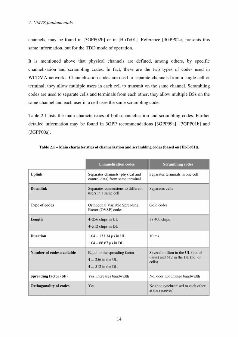
Table 2.1 lists the main characteristics of both channelisation and scrambling codes. Further
detailed information may be found in 3GPP recommendations [3GPP99a], [3GPP01b] and
[3GPP00a].
Table 2.1 – Main characteristics of channelisation and scrambling codes (based on [HoTo01]).
Channelisation codes Scrambling codes
Uplink Separates channels (physical and control data) from same terminal
Separates terminals in one cell
Downlink Separates connections to different users in a same cell
Separates cells
Type of codes Orthogonal Variable Spreading Factor (OVSF) codes
Gold codes
Length 4–256 chips in UL
4–512 chips in DL
38 400 chips
Duration 1.04 – 133.34 µs in UL
1.04 – 66.67 µs in DL
10 ms
Number of codes available Equal to the spreading factor:
4 ... 256 in the UL
4 ... 512 in the DL
Several million in the UL (no. of users) and 512 in the DL (no. of cells)
Spreading factor (SF) Yes, increases bandwidth No, does not change bandwidth
Orthogonality of codes Yes No (not synchronised to each other at the receiver)
2. UMTS fundamentals
15
While in GSM there was the need to plan the frequencies to be used in each cell, in order to
allow efficient re-use of spectrum and simultaneously avoid interference to grow, in UMTS
that is not required – each 5 MHz carrier will be used in each cell, thus, following a 1/1
pattern. Nevertheless, scrambling codes need to be planned to conveniently separate the BSs.
2.3 Radio resource management
The use of the air interface resources is a Radio Resource Management (RRM) task of
extreme importance, which has strong impact on the fulfilment of the Quality of Service
(QoS) requirements. There are three basic aspects that need to be considered: power control,
admission control, and handover.
The power control mechanism in UMTS is not focused on selecting a priori a power level to
be used by the transmitter. Instead, it is based on a quality level (the Signal to Interference
Ratio (SIR)) that has to be achieved by transmitting with an appropriate power level; if the
SIR is too low, the received signal cannot be de-spread and reconstructed any more. Since all
users are transmitting simultaneously, the noise level depends, among others, on the number
of users. A good power control algorithm will optimise the usage of the radio resources, thus,
increase system capacity.
There are 2 types of power control:
• Open Loop Power control: it consists in setting the transmit power by measuring the path
loss of the direct link via the received signal and adding the interference level of the
Node B.
• Closed Loop Power control: it is intended to reduce interference in the system by
maintaining the quality of air interface communication as close as possible to the minimum
quality required for the type of service requested by the user.
The closed loop power control consists of two parts, an inner loop and an outer one:
• The inner part of the closed loop power control is also called fast power control (at
1500 Hz), since it is intended to respond to fast variations in propagation characteristics of
the radio link (e.g., fast-fading at slow or medium speeds) as well as rapidly changing
interference conditions. The power control loop is closed because the receiver of the radio

2. UMTS fundamentals
16
signal provides commands back to the sender to adjust its transmitted power. Fast power
control is considered to be a function of the UTRA physical layer, and it is performed in
both the Node B and the UE.�
• The outer loop power control algorithm determines the parameter level used by Layer 1 to
perform the inner loop power control decisions. The outer loop control function manages
the inner loop process by setting the SIR target parameter and the power up/down step
sizes. The frequency of the outer loop power control is typically in the range of
10 – 100 Hz.
Admission control (restrict access to more voice / data calls) and congestion control (either by
lowering bit rates of services, or by carrying out intra-frequency handovers, or even
disconnecting calls) need to be performed in order to avoid the increase of interference. Users
located on the edge of a cell are those who require from the corresponding BS more power,
and, consequently, those who should be pushed out of the cell effective coverage area. By
powering off the major interferers, an immediate interference decrease is achieved, the
transmitted power from the BS may consequently be reduced and the system becomes more
stable – more users will be further allowed to enter the cell. This is known as the cell
breathing phenomena, i.e., a reduction / increase on the size of the cell to control interference.
Handovers are mainly required when MTs are moving around. Users may be served in other
cells in a more efficient way (like lower transmission power, or less interference),
nevertheless, handovers might also be performed for other reasons, such as system load
control. There are three categories of handovers:
• Hard handover means that all the old radio links in the UE are removed before the new
radio links are established, and they can be seamless, meaning that the handover is not
perceptible to the user. In practice a handover that requires a change of the carrier
frequency (inter-frequency handover) is always performed as hard handover.
• Soft handover means that the radio links are added and removed in a way that the UE
always keeps at least one radio link to the UTRAN, and it is performed by means of macro
diversity, which refers to the condition that several radio links are active at the same time.
• Softer handover is a special case of soft handover, where the radio links that are added
and removed belong to the same Node B (i.e., the site of co-located BSs from which
several sector-cells are served). In softer handover, macro diversity with maximum ratio

2. UMTS fundamentals
17
combining can be performed in the Node B, whereas generally in soft handover on the DL,
macro diversity with selection combining is applied.
2.4 Services and applications
While estimating both coverage and capacity of a UMTS network, operators aim at
dimensioning the equipment to provide services and applications that meet users’ needs. The
notion of “service” is used within the UMTS world with a variety of meanings: at a first
glance, one would associate the word “service” to the user application, like web-browsing or
e-mail. Being more rigorous, and depicting the definitions presented in [3GPP03], it may be
said that a service is a component of the portfolio of choices offered by service providers to a
user, whereas an application is a service enabler deployed by service providers, manufacturers
or users. SMS is an example of a mobile service, while the ability to make flight bookings via
a specific provider corresponds to an example of a mobile application.
Figure 2.3 represents an example of choices of such services and applications, as defined by
the UMTS Forum [UMTS01].
Services and applications may be grouped into different classes or categories, according to
their own characteristics. The classifications presented by well known standardisation bodies,
namely ITU-T, 3GPP, ETSI and UMTS Forum, are summarised in [FMSC01]. Taking into
consideration the fact that the leading UMTS vendors are basing their equipment deployment
in 3GPP standards, the classification of services considered in this thesis is the one as
proposed by 3GPP.
The UMTS drivers will be responsible for providing to the users the most adequate set of
services and applications, by making the difference not only from the technical / quality point
of view, but also by considering the inherent economical aspects. UMTS is expected to offer
the user the provision of a contracted end-to-end QoS (throughput, transfer delay, data error);
it will be possible to negotiate and renegotiate the characteristics of a bearer service at session
or connection establishment, and during ongoing sessions or connections.

2. UMTS fundamentals
18
Figure 2.3 – Example of services and applications in UMTS (adapted from [UMTS01]).
From an end-user and application points of view, four major traffic classes with different QoS
requirements can be identified. The main characteristics of these traffic classes are listed in
Table 2.2.
Each application is always associated to a certain Radio Access Bearer (RAB). When the
terminal is being activated, the QoS profile of the application is sent and a comparison of the
attributes values with the user profile as registered in the Home Location Register (HLR) is
done, before a radio bearer is either established or not. The radio bearer attributes per traffic
class are presented in Table 2.3.
2.5 Network dimensioning
Network dimensioning is a process through which an initial estimation of the amount of
network equipment and possible configurations is determined. Key parameters of this
dimensioning phase will be coverage and capacity planning.
Conferencing:. Speech-telephony. Video-telephony. Video conferencing. Voice over IP. Teen video chat (NRT)
Location-Based:. Navigation / location. Telematics. Tracking / personal security
Information services:. Instant weather forecast. Dictionary research. Restaurant guide. Flight reservation. Virtual home environment
Financial services:. Financial / banking (E-cash). Mobile E-bill
Internet Access / Networking:. Web browsing. File download. Intranet. FTP transfers. Mobile VPN
Messaging:. Short message service. Multimedia messaging. Streaming multimedia. E-mail
Entertainment:. Internet games. Mobile music. On-line gambling
Mobile commerce:. Advertising. Transaction processing. Mobile retailing

2. UMTS fundamentals
19
Table 2.2 – UMTS traffic classes (extracted from [3GPP02a]).
Traffic class Conversational Streaming Interactive Background
Type of traffic Real Time Real Time Best Effort Best Effort
Fundamental characteristics
- Preserve time relation (variation) between information entities of the stream
- Conversational pattern (stringent and low delay)
- Preserve time relation (variation) between information entities of the stream
- Request response pattern
-Preserve payload content
-Destination is not expecting the data within a certain time
-Preserve payload content
Transfer delay requirements
<< 1 s < 1 s < 10 s > 10 s
Examples of the application
Voice, video telephony, video games
Multimedia, video on demand, webcast
Web browsing, network gaming, Telnet
Email delivery, SMS, Downloading of databases
With respect to coverage planning, there are four basic aspects that require analysis:
coverage regions, area type information, propagation conditions, and link budget. The
coverage region is either a licence obligation or an operator’s strategic decision. The area
type information results from both geographic and demographic information. The
propagation conditions need to be completely identified, in order to avoid unexpected
propagation behaviours and results. By knowing those, the related parameters may be
adjusted in the planning tools and the channel model used within its validation limits. Link
budgets are used to calculate maximum propagation losses (detailed examples of link budget
calculations may be found in [HoTo01]). The main inputs required are:
- Interference margin (inter- and intra-cell);
- Fast-fading margin;
- Soft handover gain;
- MT characteristics (maximum transmit power, antenna gain, body loss);
- BS characteristics (noise figure, antenna gain, required Signal-to-Noise Ratio (SNR),
cable losses);
- Assumptions on cell loading and applications (services) offered.

2. UMTS fundamentals
20
Table 2.3 – Radio bearer attributes per UMTS QoS class (as defined in [3GPP02a]).
Traffic class Conversational Streaming Interactive Background
Maximum bit rate X X X X
Delivery order X X X X
Maximum Service Data Unit (SDU) size
X X X X
SDU format information X X
SDU error ratio X X X X
Residual bit error ratio X X X X
Delivery of erroneous SDUs X X X X
Transfer delay X X
Guaranteed bit rate X X
Traffic handling priority X
Allocation/Retention priority X X X X
The obtained path losses are converted into cell radiuses for different environments, from
which the typical coverage areas may be derived, as well as a rough estimation of number of
sites per environment area.
After predicting the coverage area, the complex activity of site acquisition – field activity and
site negotiation – needs to be performed. Sometimes, the search area needs to be enlarged due
to the non-possibility to position the BS in the most suitable site location. After having the
definitive positions of the BSs, new predictions of the coverage areas may be obtained from
the planning tools, and, if any further parameter adjustment is required, network optimisation
will follow.
In terms of capacity planning, three main aspects need to be analysed: spectrum availability,
subscriber growth forecast, traffic density information. The spectrum available in Portugal
corresponds to 4 paired carriers (FDD) and 1 unpaired carrier (TDD) per UMTS operator, as
mentioned in Section 2.2. Operators may start by using exclusively one FDD carrier all over
2. UMTS fundamentals
21
the network, as long as the generated traffic does not increase, or already introduce more
spectrum right from the beginning. FDD carriers may be used on a hierarchical cell structure,
covering umbrella, macro-, micro- or pico-cells, while TDD spectrum is mainly planned to
cover hot spot areas, where low mobility is necessary, but capacity for asymmetric traffic with
high bit rates is required. Subscriber growth forecasts result from marketing projections.
Traffic density information for UMTS networks is still non-existing, the currently required
figures being estimated as long as real values are not available.
Capacity dimensioning in UMTS is a very complex task. It depends not only on the three
aspects mentioned above, but also on other parameters like:
- Interference and noise (depend on cell loading, frequency reuse and sectorisation
efficiency);
- UL pole capacity (depends on the mixed service rates considered – target SNR and
processing gain);
- DL capacity and transmitted Equivalent Isotropic Radiated Power (EIRP) (depend on
the link balance and on the power per traffic channel).
It will basically correspond to the number of active links that achieve, in a given coverage
area and at a specific time instant, the QoS requirements in an antenna sector.
Capacity dimensioning in GSM is a completely different task. The area to be covered is
overlaid with a regular cell pattern, the available spectrum (40 frequencies in the 900 MHz
and another 40 in the 1800 MHz band, per operator, in Portugal) is distributed among a group
of cells (cluster) and then repeated all over the network, bearing in mind that a good
compromise between minimisation of adjacent channel interference and maximisation of
traffic capacity has to be attained. When more capacity is required, a couple of additional
actions can be undertaken, if no more spectrum is available: change of cell pattern, cell
splitting, frequency borrowing from neighbouring cells, use of overlaid / underlaid cells, or
cell sectorisation. System capacity depends mainly on the available spectrum and on the
interference caused by adjacent channels, and can easily be estimated.
There is almost no experience with data over CDMA networks, and the user’s behaviour is
also still unknown. Before 3G operators are able to collect real values that allow more

2. UMTS fundamentals
22
consolidated conclusions, two main aspects may be considered for the estimation of traffic
figures required for network dimensioning:
• Prediction of the total number of users per service type and per geographical area
It will not be enough to know the traffic per cell, as it was the case in GSM: in UMTS, it
is even required to know the traffic distribution inside the cell, since it affects intra-cell
interference. Rough traffic distributions may be obtained by using district information
(where, among others, population, income and business are known) and clutters (used to
distribute traffic within districts).
• Prediction of the usage for each service type
Up to now, the user profile and his/her needs in terms of service types required were
obtained through marketing studies. It is expected that, if an attractive set of applications
is offered to the user at a reasonable price, an increase on the use of 3G may occur. The
creation of new services and user needs will be a major point in the success of the
introduction of 3G, although some uncertainty on the real behaviour of the 3G users is still
present.
Among others, the MT speed, multipath channel profile, power control, handover, bit rate and
type of services, play a more important role in WCDMA systems than in 2G TDMA/FDMA
systems. A growth on the number of users, or simply on the transmission data rates within a
certain coverage area, is power demanding and may cause an increase in the overall
interference, meaning that other users (especially those more distant from the BS) may see
their requirements affected / restricted.
As in WCDMA all users share the same interference resources in the air interface, they cannot
be analysed independently: each user influences the others and causes others’ transmission
powers to change. Therefore, the whole prediction process required to complete the UMTS
radio network planning has to be done iteratively, until transmission powers stabilise.
The traffic models that shall be considered need to be able to reflect the various characteristic
features of the upcoming UMTS services, namely real-time and non-real-time. Further
analysis on the identification of adequate traffic models for UMTS, considering voice and
data services over CS and PS domains, as well as a description of the interdependent

2. UMTS fundamentals
23
parameters, like system capacity, coverage and interference, are done in detail in the
following chapter.

24
25
3 Traffic analysis
3.1 Coverage estimation
In UMTS, coverage, capacity and QoS planning are items that depend on each other and
support the overall network planning process. The cell radius in UMTS is a factor that
depends, among others, on the traffic allowed inside the cell, meaning that a complex cell
range analysis is required in order to achieve an accurate dimensioning (equipment and
configuration) of the network.
The first key element required for this complex radio network planning process is the link
budget estimation – it is used to derive the maximum path loss allowed between the UE and
the Node B, leading to a first indicative maximum cell radius that meets the quality objectives
defined in advance, and allows a rough estimation of the required network elements (CN
elements, RNCs, Node Bs, and others). Operators’ requirements, like areas to be covered,
subscriber and traffic forecasts, throughput, blocking probability (for CS) or maximum
allowed delay or loss per type of service (for PS), are inputs that need to be clearly specified
prior to the final dimensioning of the network.
Three distinct situations are evaluated hereafter for service rates at 12.2, 64, 128 and
384 kbps:
• Vehicular: MTs moving at 120 km/h on suburban environments, where users are located
inside cars (in-car loss and exclusive data terminals considered); no fast-fading margin
will be taken into account due to the impossibility to compensate, at that speed, for the
fast power control;
• Pedestrian: MTs moving at 3 km/h on metropolitan centres / large cities, where users
walk around on streets;
• Indoor: MTs moving as well at 3 km/h on metropolitan centres / large cities, but located
inside buildings – an additional building penetration margin is considered for this
particular situation, as it is assumed that coverage is provided by outdoor BSs.

3. Traffic analysis
26
Both UL and DL link budgets are calculated, aiming at concluding if there is any of these
connections that systematically impose a restriction on the coverage area (radius of the cell).
The allowed propagation loss for the cell range is given by [HoTo01]:
[dB] [dBm] [dBi] [dB] [dBm] [dBi] [dB] [dB] [dB]
[dB] [dB] [dB] [dB]
p t t c r min r div SHO body loss
log normal fast fading in car building
L P G L P G G G M
M M L L−
− − −
= + − − + + + −
− − − −
(3.1)
where:
• Pt Transmission power
• Gt Antenna gain at the transmission
• Lc Cable losses in the BS
• Pr min Receiver sensitivity
• Gr Antenna gain at the reception
• Gdiv Diversity gain
• GSHO Soft-handover gain
• Mbody-loss Body loss margin
• Mlog-normal Log-normal fading margin
• Mfast-fading Fast-fading margin
• Lin-car In-car loss
• Lbuilding Building penetration loss
The resulting propagation losses obtained on both UL and DL connections are the input
values required for the cell radius calculations. An appropriate propagation model is selected
and, consequently, the maximum cell radius is derived.
As with GSM, the user interfaces to the RNCs are not completely specified within the 3GPP
standards, meaning that distinct vendors may use slightly different parameter settings. The
particular UMTS link budget parameter values used on the link budget calculations are
summarised hereafter.
Both UMTS MT and BS characteristics differ from those used in GSM. The assumptions
presented in Table 3.1 are recommended by the most well-known vendors, which are used in
the next section for the link budget calculations:

3. Traffic analysis
27
Table 3.1 – MTs and BSs assumptions (based on [HoTo01]).
Mobile Terminals Speech terminals Data terminals
Maximum transmission power (Pt [dBm]) 21 24
Antenna gain (Gt [dBi] or Gr [dBi]) 0 2
Body loss margin (Mbody-loss [dB]) 3 0
Noise figure (FN [dB]) 7 7
Base Stations
Maximum transmission power (Pt [dBm]) 43
Antenna gain (Gr [dBi] or Gt [dBi]) (3-sector BS) 18
Cable losses (Lc [dB]) 2
Noise figure (FN [dB]) 5
There are four power classes that define the nominal UE maximum output power, Pt, as
specified in [3GPP01c]: class 1 with 33 dBm, class 2 with 27 dBm, class 3 with 24 dBm, and
class 4 with 21 dBm. Classes 3 (for data services) and 4 (for voice) will be the ones to be
considered, as they correspond to the most stringent values and are expected to correspond to
the majority of the terminals that will enter the market.
The MT antenna gain, Gt or Gr, considered in [HoTo01] is 0 dBi for terminals with data and
voice capabilities, and 2 dBi for MT exclusively oriented towards data services (where
different antennas, with slightly higher gains, may be built in).
A 3 dB body loss margin, Mbody-loss, is assumed when the MT is used for voice services, as its
position will mainly be close to the user’s head and the signal absorption is higher. When this
same terminal is used for data services, it is assumed that the user is holding it on his/her
hand, body absorption being negligible.
A 5 dB noise figure, FN, is considered for the BS (parameter that corresponds to the reception
level above the noise level), whereas 7 dB is assumed for the MT noise figure.
The ratio Eb/N0, energy per bit over noise spectral density, corresponds to another parameter
that needs to be considered, which is commonly obtained through complex simulations; the
values used for the link budget calculations are extracted from [FCSC02], Table 3.2.
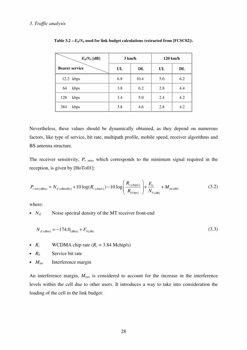
3. Traffic analysis
28
Table 3.2 – Eb/N0 used for link budget calculations (extracted from [FCSC02]).
3 km/h 120 km/h Eb/N0 [dB]
Bearer service UL DL UL DL
12.2 kbps 6.8 10.4 5.0 6.2
64 kbps 3.8 6.2 2.8 4.4
128 kbps 3.4 5.0 2.4 4.2
384 kbps 3.8 4.6 2.8 4.2
Nevertheless, these values should be dynamically obtained, as they depend on numerous
factors, like type of service, bit rate, multipath profile, mobile speed, receiver algorithms and
BS antenna structure.
The receiver sensitivity, Pr min, which corresponds to the minimum signal required in the
reception, is given by [HoTo01]:
[chip/s][dBm] [dBm/Hz] [chip/s] [dB]
[bps] 0 [dB]
10 log( ) 10 log c br min rf c int
b
R EP N R M
R N
� �= + − + +� �� �
� � (3.2)
where:
• Nrf Noise spectral density of the MT receiver front-end
[dBm] [dBm] [dB]174.0rf NN F= − + (3.3)
• Rc WCDMA chip rate (Rc = 3.84 Mchip/s)
• Rb Service bit rate
• Mint Interference margin
An interference margin, Mint, is considered to account for the increase in the interference
levels within the cell due to other users. It introduces a way to take into consideration the
loading of the cell in the link budget:

3. Traffic analysis
29
[ ] ( )dB 10log 1intM η= − −
(3.4)
where:
• η Cell load
When the cell loading increases, a larger margin is needed in the UL and, consequently, a
smaller cell radius is obtained. Typical values for the interference margin are of the order of
3 dB, corresponding to 50 % loading.
A diversity gain, Gdiv, is included as well in the estimation of the propagation loss for the cell
range, in case diversity is used on the reception of the signal. This is a feature that may be
implemented on the BS.
The soft handover gain, GSHO, takes into account the diversity gain achieved during soft
handover conditions: the receiver is allowed to compensate for both slow- and fast-fadings,
since it receives information arriving from different BSs with almost uncorrelated paths. The
typical values found in the literature for this parameter range between 2 and 4 dB. A 3 dB
value will be considered for fast moving MTs, while 1 dB less is assumed for lower speeds.
The values of the log-normal fading margin, Mlog-normal, considered in the link budget
calculations are the ones used in [HoTo01]: 7.3 dB when 95 % coverage probability is
assumed, and 4.2 dB when an 80 % coverage probability is considered. The coverage
probability corresponds to the percentage of area within the cell radius where the received
signal level exceeds a certain threshold. This parameter is related to the quality of radio
planning and radio network capacity, and depends on the variation of non-controlled
propagation elements: shadowing, penetration characteristics, fast-fading, different
environment, etc. The probability of coverage at the cell edge is one of the parameters that
define the QoS. For link budget purposes, the following thresholds are assumed:
- 95 % of coverage probability for outdoor scenarios;
- 80 % of coverage probability for indoor scenarios served by outdoor BSs.
The fast-fading margin, Mfast-fading, is included to account for the additional headroom needed
in the MT transmission power to maintain the adequate power level. This is a consequence of
the fast power control used in UMTS, and applies specifically to slow moving pedestrian
3. Traffic analysis
30
mobiles. Typical values for this parameter range between 2 and 5 dB; a 4 dB margin is
assumed for the scenarios where a slow moving MT is considered.
Penetration losses account for the type of environment in which MTs operate. The most
typical scenarios and corresponding loss values are:
- In-car (Lin-car), 8 dB
- Indoor (Lbuilding), 15 dB
Measurements for the local conditions are usually recommended, in order to use a good
estimate of the penetration losses in each environment type.
All these parameters are directly or indirectly used in link budget calculations that need to be
performed. Afterwards, an appropriate propagation model needs to be selected, in order to
describe signal propagation in particular conditions (namely for specific environments,
frequency bands, range of radius, and BS and MT heights). The maximum allowed
propagation loss calculated through (3.1) is converted by the propagation model formulation
into the maximum cell range, i.e., the area that may be served by a BS. The well-known
propagation models COST231-Okumura-Hata or COST231-Walfisch-Ikegami might be
applied.
The COST231-Okumura-Hata [DaCo99] propagation model, an empirical prediction method
for signal strength calculation, results from extensive series of measurements in and around
Tokyo at frequencies up to 1.920 MHz. Its applicability is nevertheless restricted to
frequencies up to 1.500 MHz. COST231 has extended this model to the frequency band
[1.500, 2.000] MHz by analysing Okumura’s propagation curves in the upper frequency band.
This model is usually used in macro-cells.
The COST231-Walfisch-Ikegami [DaCo99] model turns out to be a more complex model
than COST231-Okumura-Hata’s, as it allows improved path loss estimation by considering
more data describing the urban environments: building heights and separation, road widths
and orientation with respect to the direct radio path. This model is based on a deterministic
approach, and it may distinguish between line-of-sight and non-line-of-sight situations, being
usually applied to micro-cells.

3. Traffic analysis
31
Both propagation models should be calibrated for the environments where they are to be used;
after analysing the measurement results, a clutter correction factor may be required. Taking
into consideration the characteristics and applicability conditions of each of the above
mentioned propagation models, it was considered adequate to use the COST231-Walfisch-
Ikegami model for all scenarios (its complete formulation, as well as the ranges over which
these models are applicable, can be found in Annex A), since it is the one that has a lower
error in urban centre scenarios, where the larger variety of services use is expected.
The result of the application of the COST231-Walfisch-Ikegami model, in conjunction with
the allowed propagation losses obtained through (3.1), leads to the maximum cell radius on
both UL and DL connections as presented in Figure 3.1.
Vehicular Pedestrian Indoor
(a) Uplink (b) Downlink
Figure 3.1 – Cell radius.
One of the major conclusions that may be drawn after analysing the results presented above is
that macro-cell coverage is UL limited. This is basically due to the fact that the MT’s power
level is restricted to 21 dBm for voice, or 24 dBm for data terminals, instead of the 43 dBm
maximum BS transmitted power on the DL. Consequently, the coverage planning study does
not require the DL coverage information, but should consider exclusively its UL connection
characteristics, and, especially, its constraints.
Another fact that may be pointed out is the direct relationship between data rate and cell
radius: considering a fixed load / interference on the cell, as the service rates increase, the
0
1
2
3
4
5
12.2 64 128 384
Rate [kbps]
d [k
m]
0
1
2
3
4
5
12.2 64 128 384
Rate [kbps]
d [k
m]

3. Traffic analysis
32
radius of the cell shrinks. One clear exception exists for the 12.2 kbps data rate for pedestrian
and indoor users: on the UL, a maximum transmitted power of 21 dBm is considered, and a
MT antenna gain of 0 dBi is taken, together with an additional loss due to the body
absorption, leading to a slightly smaller cell radius than the obtained for the remaining service
rates considered; on the DL, the Eb/N0 value for the pedestrian and indoor scenarios is
considerably higher than the one used for the larger bit rates, leading as well to a cell radius
smaller than the ones obtained for the bit rate immediately higher. In a real network, the
dependence of the cell radius on the data rates is one of the aspects that should be closely
monitored, as new service demands may need to be kept on hold in order to avoid the “cell
breathing” phenomena to occur.
The indoor scenarios served by outdoor BSs are the most demanding ones in terms of
coverage. In order to avoid an excessive number of outdoor BSs, which reverts into an
extremely high investment, it is common to perform the coverage planning analysis solely for
outdoor environments, considering then additional indoor BSs for some indoor areas, namely
airports, exhibitions / fairs halls, business areas, shopping centres, etc..
The section that follows is dedicated to a capacity analysis, whose results need to be weighed
against the ones obtained under the current section, and further conclusions are drawn.
3.2 Capacity estimation
Another fundamental element required for the network planning process is the estimation of
the maximum number of simultaneous users that a cell can support, i.e., the system capacity.
The frequency reuse in WCDMA systems is 1, and only one 5 MHz carrier is considered here.
The system is proven to be typically interference-limited by the air interface; thus, the amount
of interference / capacity per cell must be obtained.
A capacity study on both UL and DL is presented hereafter, aiming at identifying if any of the
connections is more restrictive than the other, and extracting the limiting factors for further
calculations and comparison with the coverage analysis performed earlier. The capacity per
cell is therefore dependent on the UL and DL load factors.

3. Traffic analysis
33
The UL load factor as defined in [HoTo01] is given by:
( )1
0
11
/ 11
( / )
N
ULc b jj
b j j
iR R
E N
η
υ=
= + ⋅+ ⋅
� (3.5)
where:
• i Other cell to own interference ratio, seen by the BS (typically 65 %)
• N Number of users per cell
• Rb j Service bit rate of user j (depends on the service)
• �j Activity factor of user j at physical level (0.67 for speech and 1 for data)
The system pole capacity in the UL corresponds to the theoretical limit for the number of
MTs that a cell can cope with. At this limit, the interference level in the system is infinite and
consequently the coverage is reduced to zero. By grouping together the users into the offered
RABs, the pole capacity for the nth RAB is thus obtained when assuming an UL load factor
close to 100 %:
0
/ 11
( / )(1 )ULn
c n
b n npole
R RE N
Ni
υ+ ⋅
=+
(3.6)
where:
• Rn Service bit rate of the nth RAB (12.2, 64, 128 or 384 kbps).
The transmitted power in the UL leads to an increase on the interference to adjacent cells,
whereas the power received by MTs is considered as interference for all other users in the
same cell.
The more loaded the system is, the higher is the generated interference (as shown through
(3.4)). This implies that the receiver noise floor is greater in a highly loaded system than in an
unloaded one, as results from (3.2).
Another aspect that needs to be considered is the BSs power delivered to each user on DL; it
will basically correspond to the minimum amount of power required to establish each

3. Traffic analysis
34
connection, as it will revert in interference to other cells’ users. The BS power may be
expressed by [HoTo01]:
( )0
1
/
/
1
Nb j
rf c j p jj c jBS
TxDL
E NN R L
R RP
υ
η=
⋅ ⋅ ⋅ ⋅=
−
�
(3.7)
where:
• p jL Attenuation between BS and MT
• ηDL DL load factor
By knowing the users’ locations, it is possible to check the amount of power that a given
scenario is requesting to each BS, and if there is enough power to deliver to all users (based
on the value set up by the operators, e.g., the one presented in Table 3.1). When a
considerable number of users is no longer closely located to the BS, they will require more
power to the BS, and this will revert in interference to other users either in that cell or
neighbouring ones. The system may, thus, turn to be limited due to the “lack” of BS power.
The DL load factor, also defined in [HoTo01], is obtained through:
( )0
1
( / )1
/
Nb j
DL jj c j
E Ni
R Rη υ α
=
� = ⋅ ⋅ − + �� (3.8)
where:
• α Average orthogonal factor in the cell (depends on the multipath propagation,
ranging from 1, fully orthogonal, up to 0; the values considered hereafter
correspond to 60 % for vehicular and 90 % for pedestrian)
The pole capacity per cell in the DL is also obtained when assuming a DL load factor of
100 %:

3. Traffic analysis
35
( )0
/ 1 1( / ) 1DLn
c npole
b n n
R RN
E N i υα= ⋅ ⋅
� − + �
(3.9)
The air interface capacity in the DL is directly determined by the required transmission
power. As the BS transmission power increases, more interference is generated in the system
and less capacity will be available for MTs. In order to overcome this limitation, it is
necessary to reduce to the maximum possible extent the BS transmitted power per link,
leading to an interference reduction and an increase in system capacity.
Figure 3.2 shows the maximum path loss vs. the throughput on both UL and DL, for each of
the RAB under study (12.2, 64, 128 and 384 kbps), considering two different scenarios –
vehicular and pedestrian; the indoor scenario is left out of this analysis, as its coverage
requirements are too stringent if outdoor BSs are to be used, and its inclusion would lead to an
over dimensioning of the network.
Each plot is based on the assumption that there is a unique RAB; the throughput is obtained
by increasing the number of users until the system is 100 % loaded; the system load is used as
an input to obtain the maximum path loss, from which the cell radius may be derived. The
throughput values correspond to the product of the RAB and the number of users. This is
clearly a study case, in order to further understand the relationship between capacity and
coverage, as well as the parameters that influence those two aspects.
With respect to both UL and DL curves, the starting maximum path loss (lowest system load)
for the vehicular and the pedestrian scenarios differ slightly due to the variation on the link
budget parameters considered: Eb/N0, Mfast-fading, Lin-car and GSHO. By analysing the UL curves,
it is visible that while the load increases, the pole capacity on the cell is approached (as said
earlier, this is a theoretical value as it would lead to an infinite system interference level and a
null coverage). It is also possible to observe that an increase on the RAB on the UL leads to a
higher load value supported by the system. There is one exception to this, the 12.2 kbps case,
which receives the weigh of an activity factor lower than 1, namely 0.67, influencing
positively the overall system load.
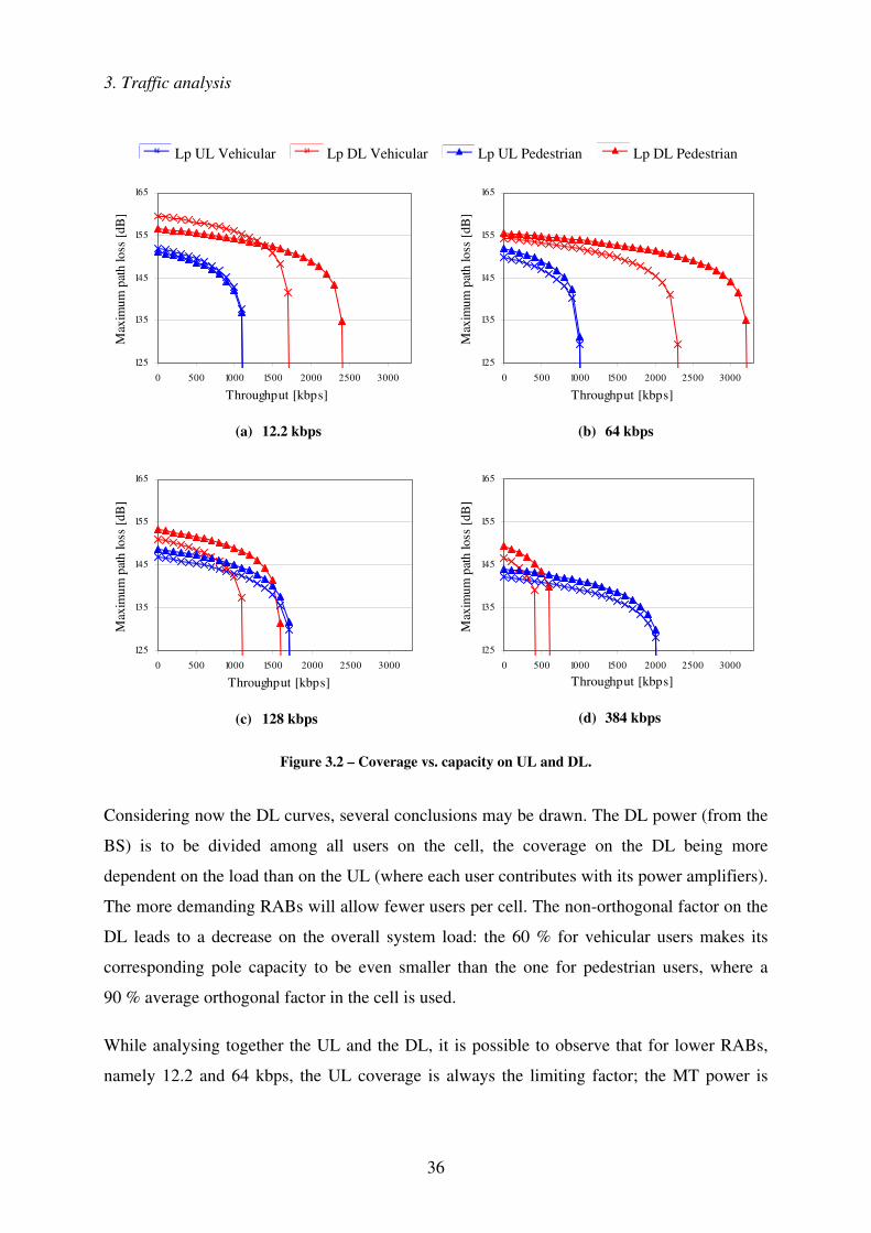
3. Traffic analysis
36
Lp UL Vehicular Lp DL Vehicular Lp UL Pedestrian Lp DL Pedestrian
125
135
145
155
165
0 500 1000 1500 2000 2500 3000
Throughput [kbps]
Max
imum
pat
h lo
ss [d
B]
(a) 12.2 kbps
125
135
145
155
165
0 500 1000 1500 2000 2500 3000
Throughput [kbps]
Max
imum
pat
h lo
ss [d
B]
(b) 64 kbps
125
135
145
155
165
0 500 1000 1500 2000 2500 3000
Throughput [kbps]
Max
imum
pat
h lo
ss [d
B]
(c) 128 kbps
125
135
145
155
165
0 500 1000 1500 2000 2500 3000
Throughput [kbps]
Max
imum
pat
h lo
ss [d
B]
(d) 384 kbps
Figure 3.2 – Coverage vs. capacity on UL and DL.
Considering now the DL curves, several conclusions may be drawn. The DL power (from the
BS) is to be divided among all users on the cell, the coverage on the DL being more
dependent on the load than on the UL (where each user contributes with its power amplifiers).
The more demanding RABs will allow fewer users per cell. The non-orthogonal factor on the
DL leads to a decrease on the overall system load: the 60 % for vehicular users makes its
corresponding pole capacity to be even smaller than the one for pedestrian users, where a
90 % average orthogonal factor in the cell is used.
While analysing together the UL and the DL, it is possible to observe that for lower RABs,
namely 12.2 and 64 kbps, the UL coverage is always the limiting factor; the MT power is

3. Traffic analysis
37
very low and it does not allow the user to be too distant from the BS. The system itself does
not show any restriction in terms of capacity for lower RABs. On the other hand, for higher
RABs, 128 and 384 kbps, an intersection on the UL and DL curves is visible on Figure 3.2.
This means that, for higher data rates but low system load, the UL coverage is still the most
severe factor to be considered on the dimensioning, whereas the DL capacity is the aspect that
will restrict the system when an increasing number of users are to be served. This is due to the
fact that the BS transmission power, despite of being considerably higher than the MT’s one
(critical factor on low load), has to be divided among all users.
Real scenarios involve all service types at the same time, both on UL and DL, with potentially
asymmetric traffic on the two links. Each service is mapped onto the most adequate RAB, as
defined by the operators.
3.3 Code planning
It is mentioned in Section 2.2 that there are two types of operations that affect the physical
channels in UMTS: channelisation and scrambling.
The channelisation operation allows the transformation of each bit into a SF number of chips,
by increasing the bandwidth of the signal. It uses the Orthogonal Variable Spreading Factor
(OVSF) codes, aiming at preserving the orthogonality of the user’s different physical
channels. The OVSF codes can be defined using the code tree presented in Figure 3.3.
Figure 3.3 – Code-tree for generation of OVSF codes (extracted from [3GPP01b]).

3. Traffic analysis
38
In the UL, the channelisation codes separate physical and control channels from one same
terminal; in the DL, they make the distinction between the DL connections to different users
in the same cell. The number of channelisation codes depends directly on the SFs, which are
related to the channel bit rates: they may vary between a SF of 4 (960 kbps) and 256 (15
kbps) in the UL, and a SF of 4 (1920 kbps) and 512 (15 kbps) in the DL. The utilisation of a
specific code causes the unavailability of the sub-tree of higher SFs descending from that
code, meaning that a limit on the number of channelisation codes is imposed mainly by high
bit rate services with low spreading factors. As there are some restrictions on the use of a 512
SF in case soft handover needs to be performed, it is common to use only SFs up to 256 in the
DL; this upper limit will as well be used in this thesis.
The scrambling operation corresponds to the application of “scrambling” codes (Gold
sequence of 38.400 chips) to the spread signal, and is used to distinguish among terminals in
one cell in the UL, or cells from each other in the DL. There are 224 scrambling codes
available in the UL, meaning that there is a very remote chance that all these codes are used.
The maximum number of scrambling codes in the DL is a little bit smaller, i.e., 218-1.
Nevertheless, not all of these DL codes may be employed – the scrambling codes that are
used are divided into 512 sets of primary codes, each one encompassing 15 secondary
scrambling codes. This makes a total of 512 × 15 codes, i.e., 7.680. Each cell receives only
one primary code in the DL, meaning that in total only 512 cells may be distinguished – 512
correspond to the scrambling code reuse factor. The P-CCPCH uses always a primary
scrambling code, while the other DL physical channels use either the primary or the
secondary scrambling codes associated with the primary scrambling code that identifies the
cell.
Especially in the DL, it has to be confirmed if the number of available channelisation codes is
limiting the system capacity or not. Considering the set of services presented in [FCSC02],
which is further used in the next chapters, the corresponding SFs and numbers of codes,
Table 3.3, determine the number of users in the system, Figure 3.4; the channel bit rate is
obtained through:
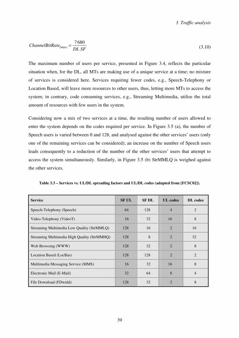
3. Traffic analysis
39
[kbps]
7680ChannelBitRate
DL SF= (3.10)
The maximum number of users per service, presented in Figure 3.4, reflects the particular
situation when, for the DL, all MTs are making use of a unique service at a time; no mixture
of services is considered here. Services requiring fewer codes, e.g., Speech-Telephony or
Location Based, will leave more resources to other users, thus, letting more MTs to access the
system; in contrary, code consuming services, e.g., Streaming Multimedia, utilise the total
amount of resources with few users in the system.
Considering now a mix of two services at a time, the resulting number of users allowed to
enter the system depends on the codes required per service. In Figure 3.5 (a), the number of
Speech users is varied between 0 and 128, and analysed against the other services’ users (only
one of the remaining services can be considered); an increase on the number of Speech users
leads consequently to a reduction of the number of the other services’ users that attempt to
access the system simultaneously. Similarly, in Figure 3.5 (b) StrMMLQ is weighed against
the other services.
Table 3.3 – Services vs. UL/DL spreading factors and UL/DL codes (adapted from [FCSC02]).
Service SF UL SF DL UL codes DL codes
Speech-Telephony (Speech) 64 128 4 2
Video-Telephony (VideoT) 16 32 16 8
Streaming Multimedia Low Quality (StrMMLQ) 128 16 2 16
Streaming Multimedia High Quality (StrMMHQ) 128 8 2 32
Web Browsing (WWW) 128 32 2 8
Location Based (LocBas) 128 128 2 2
Multimedia Messaging Service (MMS) 16 32 16 8
Electronic Mail (E-Mail) 32 64 8 4
File Download (FDwnld) 128 32 2 8
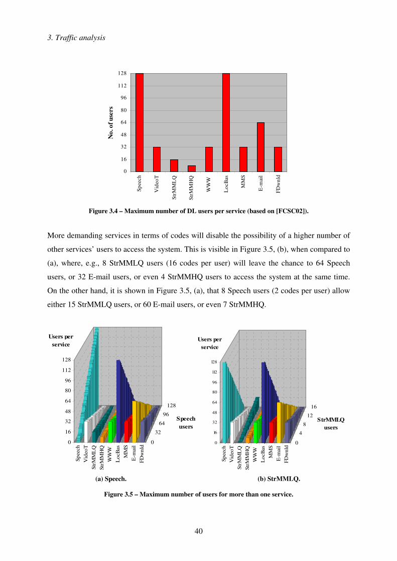
3. Traffic analysis
40
0
16
32
48
64
80
96
112
128
Spee
ch
Vid
eoT
StrM
ML
Q
StrM
MH
Q
WW
W
Loc
Bas
MM
S
E-m
ail
FDw
nld
No.
of u
sers
Figure 3.4 – Maximum number of DL users per service (based on [FCSC02]).
More demanding services in terms of codes will disable the possibility of a higher number of
other services’ users to access the system. This is visible in Figure 3.5, (b), when compared to
(a), where, e.g., 8 StrMMLQ users (16 codes per user) will leave the chance to 64 Speech
users, or 32 E-mail users, or even 4 StrMMHQ users to access the system at the same time.
On the other hand, it is shown in Figure 3.5, (a), that 8 Speech users (2 codes per user) allow
either 15 StrMMLQ users, or 60 E-mail users, or even 7 StrMMHQ.
0
32
64
96
128
Spee
chV
ideo
TSt
rMM
LQ
StrM
MH
QW
WW
Loc
Bas
MM
SE
-mai
lFD
wnl
d
0
16
32
48
64
80
96
112
128
Users per service
Speechusers
0
4
8
12
16
Spee
chV
ideo
TSt
rMM
LQ
StrM
MH
QW
WW
Loc
Bas
MM
SE
-mai
lFD
wnl
d
0
16
32
48
64
80
96
112
128
Users per service
StrMMLQ users
(a) Speech. (b) StrMMLQ.
Figure 3.5 – Maximum number of users for more than one service.

3. Traffic analysis
41
The possible combinations of each type of service (considering the required codes) to
complete the amount of DL available codes is high, but the effective number of users is
relatively limited. One possible way to overcome the lack of these codes, in order to increase
the number of users in the system, is to use more than one code tree, combined with distinct
scrambling codes. It is thus possible to assign up to 15 code trees (secondary scrambling
codes) per cell, reducing significantly the possibilities to run out of codes.
3.4 General traffic aspects
In UMTS, real-time and non-real-time services need to be handled in a different way: real-
time (conversational and streaming) use the CS part of the network, to guarantee that there are
no unacceptable delays on the provision of the services, whereas non-real-time (interactive
and background) may be satisfied through the PS part, as they can wait until there are
resources available on the network and support delivery delays.
CS traffic is characterised through four main parameters: call arrival patterns (usually
random, modelled by a Poisson process), blocked calls (calls that cannot be completed at the
time of request, due to congestion, and that are lost or held in a queue), number of channels
(the resource that has to be shared among users) and holding times (average call duration). In
order to optimise the available resources, the CS traffic should be limited to symmetrical
services, i.e., the same amount of traffic on UL and DL. The traffic models with widest
adoption in 2G are Erlang-B, Erlang-C and Engset (see, e.g., [Rapp96] and [Yaco93]).
PS traffic needs a different characterisation with respect to the CS one, as it is usually of an
asymmetric nature and arrives in bursts. A packet service session may be further characterised
through the following parameters, in order to reflect its typical behaviour [ETSI98]: session
arrival process (how data packets arrive to the system, usually modelled as a Poisson
process), number of packet transmissions per session (typically a Geometrically distributed
random variable), reading time between packet transmissions (a Geometrically distributed
random variable as well), number of packets within a session (different statistical distributions
can be used to generate the number of packets that better describe each traffic case; it is
common to use the Geometrical distribution to determine this parameter), its inter-arrival
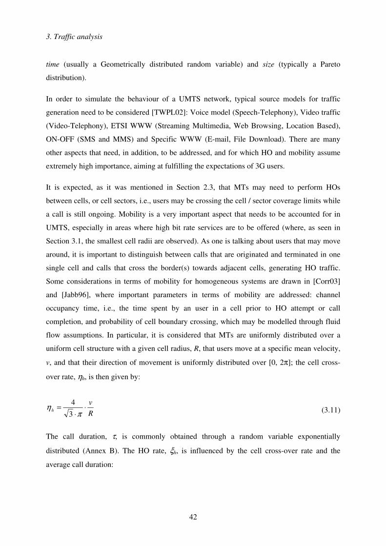
3. Traffic analysis
42
time (usually a Geometrically distributed random variable) and size (typically a Pareto
distribution).
In order to simulate the behaviour of a UMTS network, typical source models for traffic
generation need to be considered [TWPL02]: Voice model (Speech-Telephony), Video traffic
(Video-Telephony), ETSI WWW (Streaming Multimedia, Web Browsing, Location Based),
ON-OFF (SMS and MMS) and Specific WWW (E-mail, File Download). There are many
other aspects that need, in addition, to be addressed, and for which HO and mobility assume
extremely high importance, aiming at fulfilling the expectations of 3G users.
It is expected, as it was mentioned in Section 2.3, that MTs may need to perform HOs
between cells, or cell sectors, i.e., users may be crossing the cell / sector coverage limits while
a call is still ongoing. Mobility is a very important aspect that needs to be accounted for in
UMTS, especially in areas where high bit rate services are to be offered (where, as seen in
Section 3.1, the smallest cell radii are observed). As one is talking about users that may move
around, it is important to distinguish between calls that are originated and terminated in one
single cell and calls that cross the border(s) towards adjacent cells, generating HO traffic.
Some considerations in terms of mobility for homogeneous systems are drawn in [Corr03]
and [Jabb96], where important parameters in terms of mobility are addressed: channel
occupancy time, i.e., the time spent by an user in a cell prior to HO attempt or call
completion, and probability of cell boundary crossing, which may be modelled through fluid
flow assumptions. In particular, it is considered that MTs are uniformly distributed over a
uniform cell structure with a given cell radius, R, that users move at a specific mean velocity,
v, and that their direction of movement is uniformly distributed over [0, 2π]; the cell cross-
over rate, ηh, is then given by:
Rv
h ⋅⋅
=π
η3
4 (3.11)
The call duration, τ, is commonly obtained through a random variable exponentially
distributed (Annex B). The HO rate, ξh, is influenced by the cell cross-over rate and the
average call duration:

3. Traffic analysis
43
h hξ η τ= ⋅ (3.12)
The completed calls, µ, known as well by service time, may be obtained by knowing the
average call duration:
τµ 1= (3.13)
The average dwell time, τh, also known as residence time in a cell, is given by the inverse of
the cell cross-over rate:
hh η
τ 1= (3.14)
Another important and useful relation is the mean channel occupancy time in a cell, τc, which
is given by:
1c
h
τµ η
=+
(3.15)
The mean arrival rate, λ, corresponds to the sum of both new calls, λn, and HO calls, λh, the
system entries being:
n hλ λ λ= + (3.16)
The amount of traffic per user, represented henceforth by A, for c servers, is given by:
Acλµ
=⋅
(3.17)
In any communication system, channels need to be shared among many users. Users’
demands are placed randomly, and the call duration has usually an unpredictable duration. As
some requests may arrive while all resources are in use, it is required to define a general
access mechanism to the available channels: Figure 3.6 shows how the general call access

3. Traffic analysis
44
mechanism for voice through CS is accomplished. Afterwards, a similar access mechanism of
a queuing system fitting PS purposes is presented.
Figure 3.6 – General call access mechanism for CS (extracted from [Corr03]).
Part of the total system resources, C channels, is used for both new generated and HO calls,
Cg, while the remaining ones, Ch, are allocated exclusively to handover calls.
g hC C C= + (3.18)
If, at any instant, a CS user arrives to the system and there is no available resources, the call
cannot be completed and will be either held (kept in a queue, if there is one), or lost (blocked,
in case of a new user, Pb, or failed, for a HO user, Phf). The probabilities of blocking calls and
handover failure are given by [Jabb96]:
1
0
!
! !
g
g
g
g g
g
g
k CCC h
k C
b C k Ck CC h
k k C
AA
kP
AAA
k k
−
=− −
= =
=+
�
� � (3.19)
1
0
!
! !
hg
g g
g
g
CC h
hf C k Ck CC h
k k C
AA
CPAA
Ak k
− −
= =
=+� �
(3.20)
3. Traffic analysis
45
where Ah is the traffic load due exclusively to HO. New and HO calls will be dealt with in the
same way, leading to Phf = Pb.
Another arising probability that affects the call behaviour is the drop call probability, Pd,
which occurs when there are calls lost in HO; this probability is given by [Jabb96]:
( )1 1h hf
dh hf
P PP
P P=
− − (3.21)
Ph is the probability of performing HO and can be obtained through:
( )h
h
h
chhP
ηµη
ττττ
+==>= Prob (3.22)
The HO call rate, λh, is given by:
( )( )1
1 1h b
h nh hf
P P
P Pλ λ
−=
− − (3.23)
In case Pb and Phf assume small values, which is usually the case, the HO call rate may be
further simplified into:
1h h
h n h n nh
PP
ηλ λ ξ λ λµ
≅ = =−
(3.24)
When the system reaches a steady-state, the HO rate at the entry is equal to the outgoing HO
rate; in steady-state, Pb may be obtained through the Erlang-B model [Leon94]:
0
!
!
C
b iC
i
ACP
Ai=
=�
(3.25)
In traditional 2G CS networks, like GSM, which were planned from the begin to provide a
unique service (voice), traffic dimensioning is based on the Erlang-B model, an M/M/c/c

3. Traffic analysis
46
queuing system according to Kendall’s classification of queuing systems (1953). The
Erlang-B model is based on the assumption that there is an infinite number of users per cell,
and it does not account for users’ mobility, thus, it does not consider handover; in addition,
calls that cannot be established due to lack of resources are simply lost. For GSM networks,
typical values for the blocking probability range between 1 and 2 %.
Similarly to what was seen for CS, a general call access mechanism for data through PS may
be established, Figure 3.7. There are now different system parameters that may be measured:
the data loss probability, L, and the mean waiting time, τw, which is a direct result of
including a buffer to store data until there are resources to serve the users. Adequate models
are, thus, required to obtain those parameter values.
Figure 3.7 – General call access mechanism for PS (adapted from [Leon94]).
A model that is commonly used to account for data is the M/G/1 queuing system, which is a
single-server system. Arrivals follow again a Poisson process, but the service times are no
longer exponentially distributed.
The mean waiting time in an M/G/1 system is given by [Leon94]:
2(1 ) 12(1 )w
A CA
ττµ
+= ⋅−
(3.26)
3. Traffic analysis
47
2Cτ being the coefficient of variation of the service time, obtained through:
( )2
22
1/C τ
τσ
µ= (3.27)
(3.26) is frequently referred to be the Pollaczek-Khinchin mean value formula.
There is another model, the Erlang-C, which corresponds to an M/M/c queuing system;
contrarily to the Erlang-B model, this one accounts for the possibility to hold in a queue all
calls that could not be served until there are available resources. The probability that a call
will wait in a queue is given by [Leon94]:
1c
w
pP
A=
− (3.28)
where pc is the probability for state c, given by:
11
0
( / ) ( / ) ( / ) 1! ! ! 1
c j cc
cj
pc j c A
λ µ λ µ λ µ−
−
=
� = ⋅ +� �−� �
� (3.29)
The mean waiting time, period of time elapsed since the customer arrives until he starts to be
served, is found from Little’s formula [Leon94]:
1/(1 )w wP
c Aµτ = ⋅
⋅ − (3.30)
It is worth to say that the system is stable and has a steady-state if A < 1, or, equivalently:
cλ µ< (3.31)
In cellular systems like GSM, a fixed amount of frequencies allocated to the service are
reused in a regular pattern of areas – usually hexagonal cells – each covered by one BS. In
order to avoid harmful interference, the same channels cannot be used in adjacent cells, and a
3. Traffic analysis
48
safety distance needs to be preserved, meaning that a careful frequency planning is required to
maximise the system capacity and the quality of the service provided to the user.
In UMTS, the frequency reuse factor is 1, and the resource that needs to be shared by users is
no longer a preset number of frequencies, but the available system capacity, which is limited
and varies according to instantaneous conditions – among the most critical, the number of
active users and their exact location in the cell, the type of services that are being required,
and the interference (intra- or inter-cells); this leads basically to a constantly changing number
of “UMTS channels”.
Thus, traffic estimation in UMTS requires the consideration of a model more complex than
the ones used in 2G, as it has to reflect the possibility of having multi-service traffic, with
different bandwidth and QoS requirements, for scenarios that are constantly varying, and, last
but not least, that account for mobility. While mixing up voice and data traffic, its complexity
becomes very high and an accurate planning turns out to be an extremely difficult task to
achieve. It would be worthwhile to consider a model that would differentiate each traffic type,
in order to better reflect all services and its characteristics, and perform a valid study of the
network behaviour. In the absence of such an optimal theoretical model for mobile
communications, the adaptation of existing ones that already account for both voice and data
traffic is a possible way to proceed with.
A traffic model that integrates voice and data calls in a mobile communications system,
considers a finite-buffer for data, accounts for mobility, and is able to adjust the boundaries of
the available resources per service type, is adapted to the particularities of UMTS, and,
therefore, studied for various scenarios and input parameters. Its detailed description is
presented in the next chapter, a further analysis in terms of system performance being the
main objective of Chapter 5.

49
4 Traffic model
4.1 Model formulation
The traffic model that is studied in detail intends to integrate voice and data services,
considers a finite-buffer to store data packets, accounts for mobility and adapts the boundaries
of the available resources to the users’ requirements, Figure 4.1. The aim of this section is to
present the general model formulation [HaLH00]; in the next section, the adaptation of the
model to UMTS is detailed, the last section containing a description of the algorithm as
implemented.
Voice
Shared
Data C d
C s
C v
Channels
Voice analysis- P b
Dataanalysis- L and T
nvλ
hvλ
vλ
dλndλ
hdλ
, ,v v vτ µ η
, ,d d dτ µ η⊕
⊕
Buffer (B )
Figure 4.1 – Traffic model for the base station (adapted from [HaLH00]).
The number of physical channels for traffic, henceforth defined as C, corresponds to a scarce
resource that needs to be shared among voice and data users. For this purpose, the available
traffic channels are divided into three components: Cv channels exclusively dedicated to voice
calls, Cd channels restricted to data packets, and Cs=C-Cv-Cd channels to be shared between
voice and data. The boundaries between these three components can be adjusted dynamically,
aiming at an efficient utilisation of the available resources and satisfying the QoS
requirements for both voice and data traffics. All channels are made available in a first-come
first-served (FCFS) basis.

4. Traffic model
50
Instead of having a preset amount of C traffic channels per BS, it is necessary to convert this
fixed parameter into a variable that is regularly updated to reflect UMTS characteristics,
namely an interference balance based on the results of the coverage and capacity calculations.
It may occur that the C traffic channels per BS are insufficient to serve all call attempts, thus,
a finite buffer with size B is considered for data traffic, where packets are queued in case the
available resources are busy. On the other hand, if the resources foreseen for voice calls are
not available, the calls will simply not be admitted by the system, i.e., they will be blocked.
The unavailability of resources for voice leads to the inevitability to have calls blocked, which
shall, for the sake of the network, be kept as small as possible. On the other hand, if data
resources are all in use while new data packets are attempting to be transmitted, a limited
amount of packets may be buffered, but delays or packet losses may occur.
Both voice calls and data packet transmissions need to be characterised through a statistical
distribution. According to [HaLH00], voice and data traffic are assumed to follow a Poisson
distribution. Voice call arrival rates, λv, including both new and HO calls, λvn and λv
h, and
data packets arrival rates, λd, including as well new and HO packets, λdn and λd
h, are given by
(4.1) and (4.2), respectively:
hv
nvv λλλ += (4.1)
hd
ndd λλλ += (4.2)
Moreover, it is assumed that the channel assignment to each of these types of calls is not
distinguishable, i.e., the system uses a non-prioritised scheme for new and HO calls.
It is considered that voice and data traffic have an Exponential service time distribution, with
means 1/µv and 1/µd, respectively. The residence time in a cell for both, voice and data, does
also follow an Exponential distribution, and its means are given by 1/ηv and 1/ηd,
respectively.
The channel occupancy time assumes as well an Exponential behaviour, with means given by
(4.3) for voice and (4.4) for data, respectively.
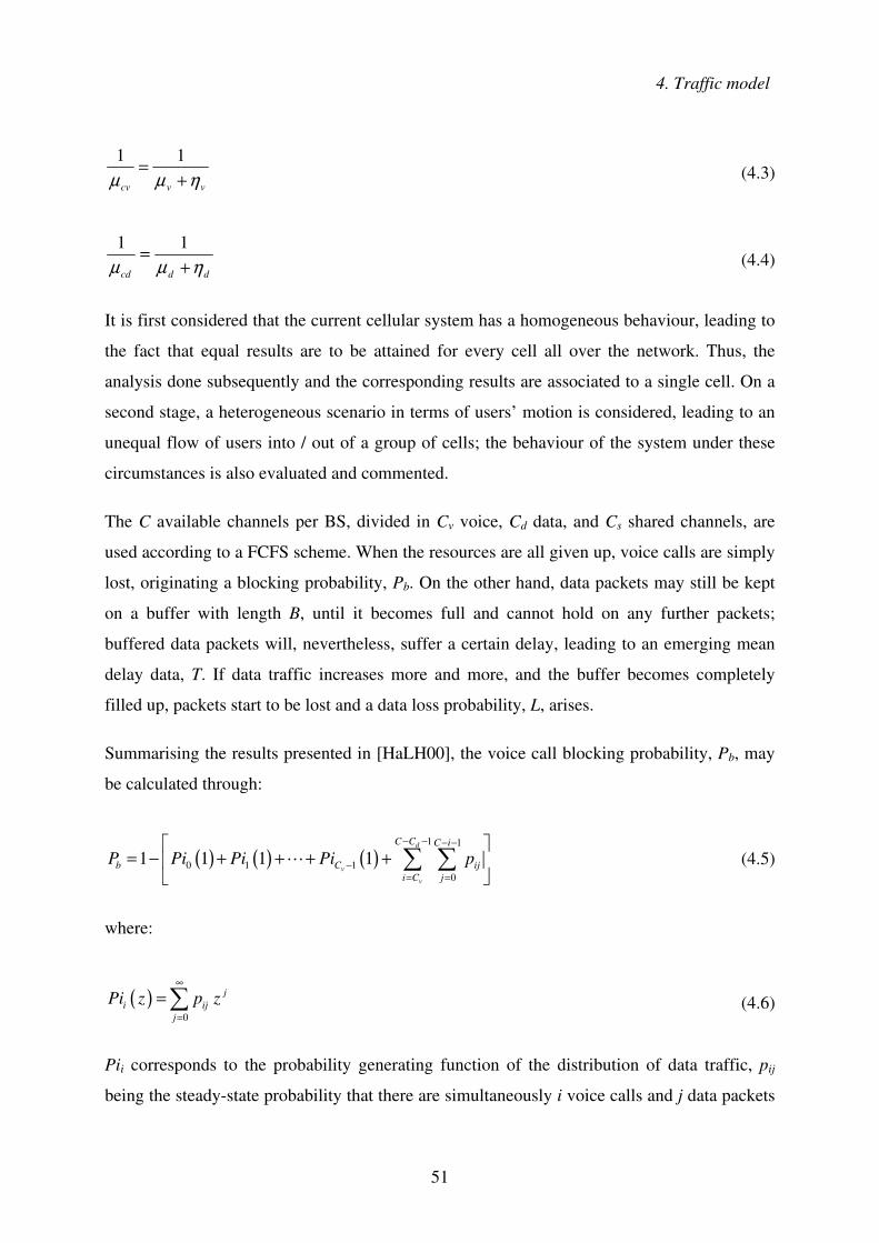
4. Traffic model
51
vvcv ηµµ += 11
(4.3)
ddcd ηµµ += 11
(4.4)
It is first considered that the current cellular system has a homogeneous behaviour, leading to
the fact that equal results are to be attained for every cell all over the network. Thus, the
analysis done subsequently and the corresponding results are associated to a single cell. On a
second stage, a heterogeneous scenario in terms of users’ motion is considered, leading to an
unequal flow of users into / out of a group of cells; the behaviour of the system under these
circumstances is also evaluated and commented.
The C available channels per BS, divided in Cv voice, Cd data, and Cs shared channels, are
used according to a FCFS scheme. When the resources are all given up, voice calls are simply
lost, originating a blocking probability, Pb. On the other hand, data packets may still be kept
on a buffer with length B, until it becomes full and cannot hold on any further packets;
buffered data packets will, nevertheless, suffer a certain delay, leading to an emerging mean
delay data, T. If data traffic increases more and more, and the buffer becomes completely
filled up, packets start to be lost and a data loss probability, L, arises.
Summarising the results presented in [HaLH00], the voice call blocking probability, Pb, may
be calculated through:
( ) ( ) ( )1 1
0 1 10
1 1 1 1d
v
v
C C C i
b C iji C j
P Pi Pi Pi p− − − −
−= =
� = − + + + +� �
�� �� (4.5)
where:
( )0
ji ij
j
Pi z p z∞
=
=� (4.6)
Pii corresponds to the probability generating function of the distribution of data traffic, pij
being the steady-state probability that there are simultaneously i voice calls and j data packets

4. Traffic model
52
in the cell under analysis, for | z | ≤ 1 and 0 ≤ i ≤ C-Cd,, computed through (4.18), to be dealt
with later.
The data loss probability, L, can be given by:
,0
dC C
i Bi
L q−
=
= � (4.7)
with:
,1
ij i j ll
q p∞
+=
=� (4.8)
qij corresponds to the tail probability of the number of data packets when there are i voice
calls in the cell.
Finally, the mean data delay, T, is obtained through:
( )
( )( )0
1
1
dC C
ii
n hd d
PiT
Lλ λ
−
=
′=
+ −
� (4.9)
where ( )1iPi ′ is obtained by differentiating (4.6):
( ) 1
1
ji ij
j
Pi z j p z∞
−
=
′ =� (4.10)
and then setting in (4.10) z = 1.

4. Traffic model
53
4.2 Adaptation of the model to UMTS
All UMTS aspects that were embedded in the traffic model under analysis are described
hereafter, as well as any further simplifications required.
One of the crucial aspects in UMTS is the amount of channels, C, that may be offered to the
user at any instant; there is here a huge difference between traditional 2G and the upcoming
3G systems, inherent to the technology chosen (TDMA vs. CDMA, respectively). The
number of channels available per cell in a 2nd generation system results from a rather simple
frequency planning activity, which requires, on one hand, the maximisation of channels per
cell, but, on the other, the reduction to the maximum extend possible of adjacent- and co-
channel interference, by increasing the re-use distance of channels. In UMTS, it is no longer
possible to talk about a fixed amount of traffic channels; there are basically three matters that
will impose restrictions to the system and, thus, limit the number of channels:
• The system load, which should not reach more than 50 % in the UL and 70 % in the DL;
• The BS power, that will be split among the users wishing to access the network, the power
required to establish the connection being dependent on the location of the user, the type of
service(s) he/she is requiring and the speed at which he is moving around;
• The existing DL codes.
The total number of voice and data channels available is, thus, dependent on instantaneous
conditions. When implementing the traffic model, three test conditions are performed before
the number of channels is estimated: if the UL and DL load limits are satisfied, by applying
(3.5) and (3.8), if the BS power is enough to satisfy all users under the cell coverage, (3.7),
and, finally, if the sum of codes required for all users, considering the service(s) under
request, is lower or equal to the ones offered by the system. If either the UL / DL load, or the
BS power, exceed the predefined values, the results from (3.5), (3.8) and (3.7) are considered
to correspond to the totality of 256 DL codes and, thus, a proportional reduction on that value
is carried out to pull down the parameter which exceeded its highest admissible value
(Figure 4.2); e.g., assuming that the DL load would have reached 85 %, the system would
allow only the use of 210 codes, according to:
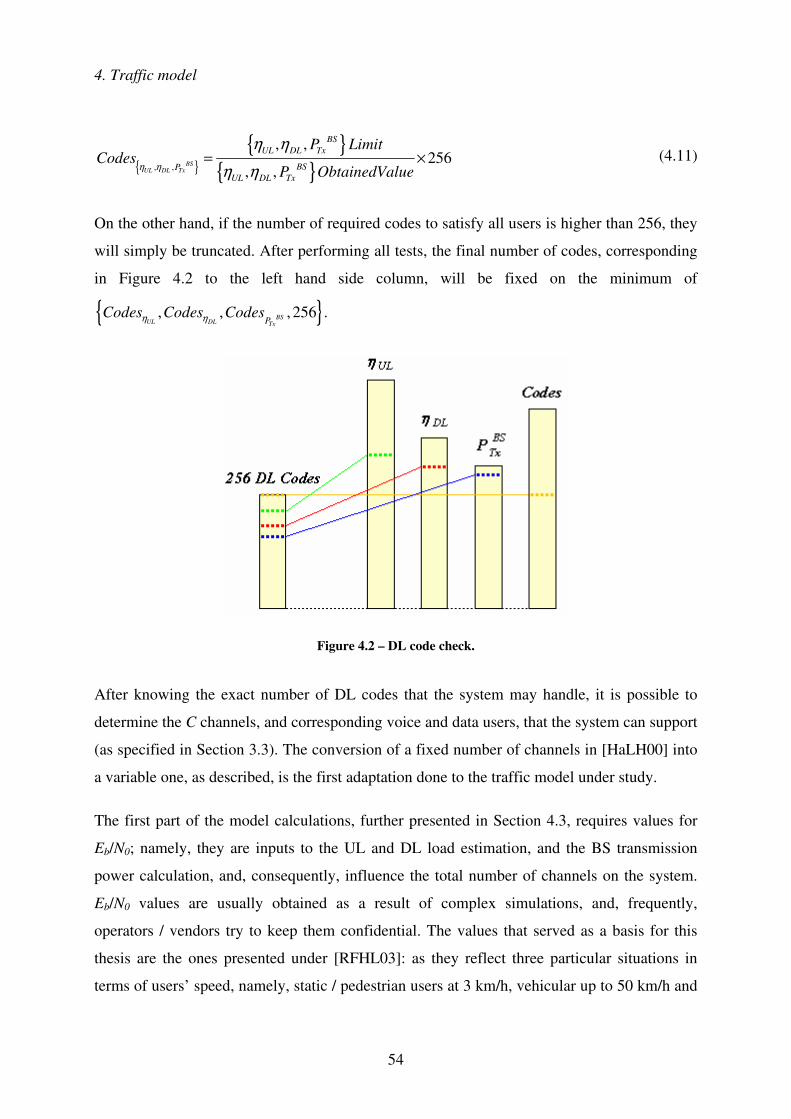
4. Traffic model
54
{ }{ }
{ }, ,
, ,256
, ,BS
UL DL Tx
BSUL DL Tx
BSPUL DL Tx
P LimitCodes
P ObtainedValueη η
η η
η η= × (4.11)
On the other hand, if the number of required codes to satisfy all users is higher than 256, they
will simply be truncated. After performing all tests, the final number of codes, corresponding
in Figure 4.2 to the left hand side column, will be fixed on the minimum of
{ }, , , 256 .BSUL DL TxP
Codes Codes Codesη η
Figure 4.2 – DL code check.
After knowing the exact number of DL codes that the system may handle, it is possible to
determine the C channels, and corresponding voice and data users, that the system can support
(as specified in Section 3.3). The conversion of a fixed number of channels in [HaLH00] into
a variable one, as described, is the first adaptation done to the traffic model under study.
The first part of the model calculations, further presented in Section 4.3, requires values for
Eb/N0; namely, they are inputs to the UL and DL load estimation, and the BS transmission
power calculation, and, consequently, influence the total number of channels on the system.
Eb/N0 values are usually obtained as a result of complex simulations, and, frequently,
operators / vendors try to keep them confidential. The values that served as a basis for this
thesis are the ones presented under [RFHL03]: as they reflect three particular situations in
terms of users’ speed, namely, static / pedestrian users at 3 km/h, vehicular up to 50 km/h and
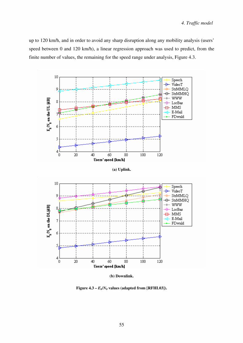
4. Traffic model
55
up to 120 km/h, and in order to avoid any sharp disruption along any mobility analysis (users’
speed between 0 and 120 km/h), a linear regression approach was used to predict, from the
finite number of values, the remaining for the speed range under analysis, Figure 4.3.
(a) Uplink.
(b) Downlink.
Figure 4.3 – Eb/N0 values (adapted from [RFHL03]).
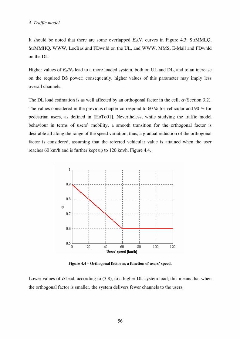
4. Traffic model
56
It should be noted that there are some overlapped Eb/N0 curves in Figure 4.3: StrMMLQ,
StrMMHQ, WWW, LocBas and FDwnld on the UL, and WWW, MMS, E-Mail and FDwnld
on the DL.
Higher values of Eb/N0 lead to a more loaded system, both on UL and DL, and to an increase
on the required BS power; consequently, higher values of this parameter may imply less
overall channels.
The DL load estimation is as well affected by an orthogonal factor in the cell, α (Section 3.2).
The values considered in the previous chapter correspond to 60 % for vehicular and 90 % for
pedestrian users, as defined in [HoTo01]. Nevertheless, while studying the traffic model
behaviour in terms of users’ mobility, a smooth transition for the orthogonal factor is
desirable all along the range of the speed variation; thus, a gradual reduction of the orthogonal
factor is considered, assuming that the referred vehicular value is attained when the user
reaches 60 km/h and is further kept up to 120 km/h, Figure 4.4.
Figure 4.4 – Orthogonal factor as a function of users’ speed.
Lower values of α lead, according to (3.8), to a higher DL system load; this means that when
the orthogonal factor is smaller, the system delivers fewer channels to the users.
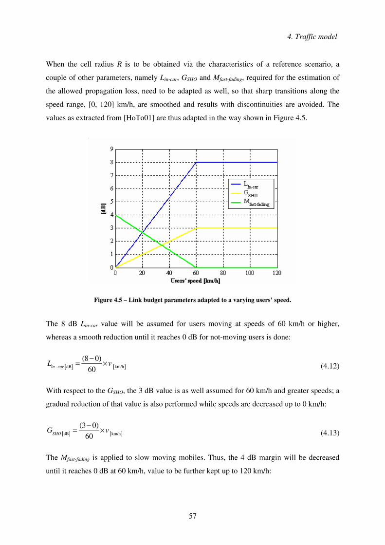
4. Traffic model
57
When the cell radius R is to be obtained via the characteristics of a reference scenario, a
couple of other parameters, namely Lin-car, GSHO and Mfast-fading, required for the estimation of
the allowed propagation loss, need to be adapted as well, so that sharp transitions along the
speed range, [0, 120] km/h, are smoothed and results with discontinuities are avoided. The
values as extracted from [HoTo01] are thus adapted in the way shown in Figure 4.5.
Figure 4.5 – Link budget parameters adapted to a varying users’ speed.
The 8 dB Lin-car value will be assumed for users moving at speeds of 60 km/h or higher,
whereas a smooth reduction until it reaches 0 dB for not-moving users is done:
[ ] [ ]dB km/h
(8 0)60in carL v−−= × (4.12)
With respect to the GSHO, the 3 dB value is as well assumed for 60 km/h and greater speeds; a
gradual reduction of that value is also performed while speeds are decreased up to 0 km/h:
[ ] [ ]dB km/h
(3 0)60SHOG v−= × (4.13)
The Mfast-fading is applied to slow moving mobiles. Thus, the 4 dB margin will be decreased
until it reaches 0 dB at 60 km/h, value to be further kept up to 120 km/h:

4. Traffic model
58
[ ] [ ]dB km/h
(0 4)4
60fast fadingM v−−= × + (4.14)
Higher values of Lin-car, obtained for users that move faster, lead to lower allowed propagation
losses (3.1), and, consequently, smaller cell radii; on the other hand, GSHO, which also
increases while users’ speed augments, leads to greater allowed propagation losses and the
cell radii are positively influenced; with respect to the Mfast-fading, as it decreases with speed
increase, the allowed propagation losses grow and cell radii expand as well, Table 4.1.
Table 4.1 – Lin-car , GSHO and Mfast-fading vs. number of channels.
v ���� Lin-car ���� Lp ���� R ���� C ����
v ���� GSHO ���� Lp ���� R ���� C ����
v ���� Mfast-fading ���� Lp ���� R ���� C ����
In order to proceed with the model calculations, it is required to find out the average voice
and data call duration values, τv and τd. For PS, it is no longer correct to refer call duration in
time units; nevertheless, the average DL session volume, as specified in Table 5.2, together
with the channel bit rates, will enable to obtain equivalent data call duration values.
The traffic model will, for the time being, use an average value for data calls, instead of
making the difference among each individual data service considered. In order to find out the
resulting average data call duration, the duration of each individual service is weighed over
the total number of users:
( )1
1
TotDataServices
i ii
d TotDataServices
ii
Users
Users
ττ =
=
×=
�
� (4.15)
If, for any reason, the selected scenario does not encompass any data user, a single average is
applied:
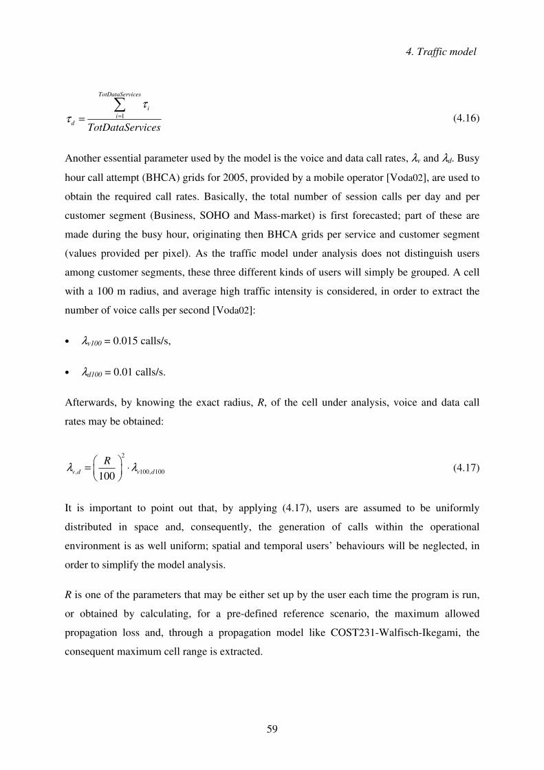
4. Traffic model
59
1
TotDataServices
ii
d TotDataServices
ττ ==
� (4.16)
Another essential parameter used by the model is the voice and data call rates, λv and λd. Busy
hour call attempt (BHCA) grids for 2005, provided by a mobile operator [Voda02], are used to
obtain the required call rates. Basically, the total number of session calls per day and per
customer segment (Business, SOHO and Mass-market) is first forecasted; part of these are
made during the busy hour, originating then BHCA grids per service and customer segment
(values provided per pixel). As the traffic model under analysis does not distinguish users
among customer segments, these three different kinds of users will simply be grouped. A cell
with a 100 m radius, and average high traffic intensity is considered, in order to extract the
number of voice calls per second [Voda02]:
• λv100 = 0.015 calls/s,
• λd100 = 0.01 calls/s.
Afterwards, by knowing the exact radius, R, of the cell under analysis, voice and data call
rates may be obtained:
2
, 100, 100100v d v d
Rλ λ� �= ⋅� �� �
(4.17)
It is important to point out that, by applying (4.17), users are assumed to be uniformly
distributed in space and, consequently, the generation of calls within the operational
environment is as well uniform; spatial and temporal users’ behaviours will be neglected, in
order to simplify the model analysis.
R is one of the parameters that may be either set up by the user each time the program is run,
or obtained by calculating, for a pre-defined reference scenario, the maximum allowed
propagation loss and, through a propagation model like COST231-Walfisch-Ikegami, the
consequent maximum cell range is extracted.
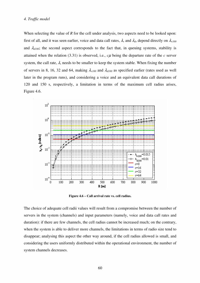
4. Traffic model
60
When selecting the value of R for the cell under analysis, two aspects need to be looked upon:
first of all, and it was seen earlier, voice and data call rates, λv and λd, depend directly on λv100
and λd100; the second aspect corresponds to the fact that, in queuing systems, stability is
attained when the relation (3.31) is observed, i.e., cµ being the departure rate of the c server
system, the call rate, λ, needs to be smaller to keep the system stable. When fixing the number
of servers in 8, 16, 32 and 64, making λv100 and λd100 as specified earlier (rates used as well
later in the program runs), and considering a voice and an equivalent data call durations of
120 and 150 s, respectively, a limitation in terms of the maximum cell radius arises,
Figure 4.6.
Figure 4.6 – Call arrival rate vs. cell radius.
The choice of adequate cell radii values will result from a compromise between the number of
servers in the system (channels) and input parameters (namely, voice and data call rates and
duration): if there are few channels, the cell radius cannot be increased much; on the contrary,
when the system is able to deliver more channels, the limitations in terms of radio size tend to
disappear; analysing this aspect the other way around, if the cell radius allowed is small, and
considering the users uniformly distributed within the operational environment, the number of
system channels decreases.

4. Traffic model
61
Neither the call rates, nor the call duration values, do influence the number of system
channels, as it is clearly seen in the next section, where the flowcharts of the implemented
algorithm are presented.
The steady-state probability that there are simultaneously i voice calls and j data packets in
the cell, pij, is a fundamental input parameter of the traffic model that is obtained analytically.
Assuming that voice and data events are independent [Meye84], it can be said that the
probability of having at the same time i and j is given by:
( ) ( ) ( )v dp i j p i p j∩ = ⋅ (4.18)
This means that the pij matrix may be obtained after knowing the individual probabilities of
each event, Figure 4.7.
0 1 2 3 ... 128
0 p v (0).p d (0) p v (1).p d (0) p v (2).p d (0) p v (3).p d (0) ... p v (128).p d (0)
1 p v (0).p d (1) p v (1).p d (1)
2 p v (0).p d (2) p v (1).p d (2)
3 p v (0).p d (3) ... ... ...
4 p v (0).p d (4) ...
... ...
128 p v (0).p d (128) p v (1).p d (128) p v (2).p d (128) p v (3).p d (128) ... p v (128).p d (128)
j (d
ata
pack
ets)
i (voice calls)
Figure 4.7 – pij matrix.
pv(i) and pd(j) may be modelled by means of a discrete random variable, such as the Binomial,
the Geometric or the Poisson one. According to [HaLH00], both voice and data calls are
Poisson distributed; this assumption is considered as well for the traffic model under analysis.
It should be added that the range of variation from i and j in Figure 4.7 comes directly from
Figure 3.4. Basically, 128 is the maximum number of users for voice and data, for particular
scenarios where users do exclusively use Speech and LocBas, respectively, these being the
less demanding services in terms of required number of codes. If other services are required
by the users, the amount of customers that may be served reduces.
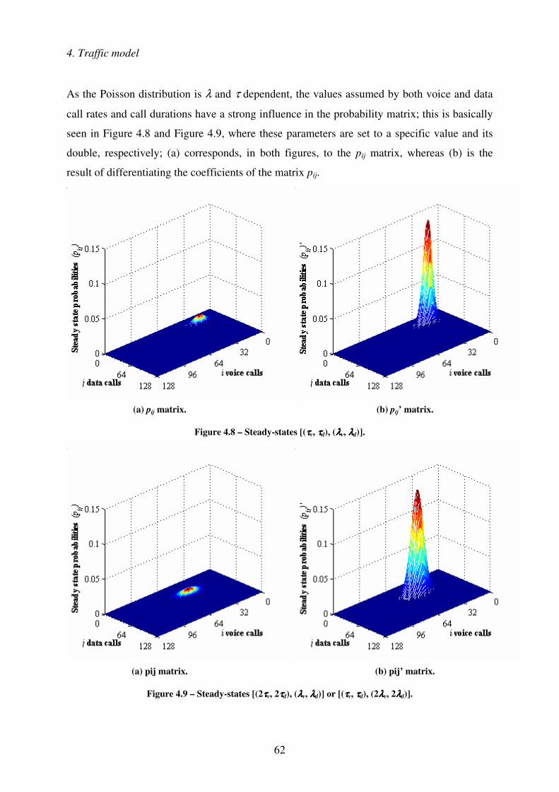
4. Traffic model
62
As the Poisson distribution is λ and τ dependent, the values assumed by both voice and data
call rates and call durations have a strong influence in the probability matrix; this is basically
seen in Figure 4.8 and Figure 4.9, where these parameters are set to a specific value and its
double, respectively; (a) corresponds, in both figures, to the pij matrix, whereas (b) is the
result of differentiating the coefficients of the matrix pij.
(a) pij matrix. (b) pij’ matrix.
Figure 4.8 – Steady-states [(ττττv, ττττd), (λλλλv, λλλλd)].
(a) pij matrix. (b) pij’ matrix.
Figure 4.9 – Steady-states [(2ττττv, 2ττττd), (λλλλv, λλλλd)] or [(ττττv, ττττd), (2λλλλv, 2λλλλd)].

4. Traffic model
63
As it can be seen in Figure 4.8 and Figure 4.9, when increasing λ or τ, the circular area that
encompasses the predominant pij and pij’ elements is a little distended, but its value is
smoothed (the sum of all pij matrix elements remains unitary); furthermore, the circular area is
slightly pushed to the centre of the pij and pij’ matrices; pij’ elements are obtained by
differentiating the pij matrix, meaning that the size of the predominant area is not changed
with respect to pij, but the individual element values are amplified considerably. A variation
of λ and/or τ implies an immediate change on the probability matrices, and, consequently, the
behaviour of the traffic model is modified, as will be seen later on.
As previously referred, pij and pij’ are modelled by a Poisson distribution, influenced by call
rate and duration values; consequently, the probability matrices will not influence the number
of channels made available by the system.
As the traffic model solely distinguishes between two types of services, i.e., voice and data,
the particularities of each data service are lost when averaging it, as mentioned earlier in this
section, to get a value to be used by the model. In order to have a better understanding on the
behaviour of a real UMTS network, it would be desirable to adapt the model to account for
the particularities of each key UMTS data service; namely, it would be worthwhile to
distinguish between the average packet size of each service, and, consequently, its equivalent
average call duration, as well as the specific data call rates. In order to do so, it would be
necessary to consider an n-dimensional space, where s would be a vector containing the set of
services, s = (s1, s2, …, sn), and s ∈ �n. The steady-state probabilities for the n number of
services considered, p1,2,…,n, would be a real-value function of n variables,
p1,2,…,n = f(s1, s2, …, sn).
The traffic model under study includes a buffer to store packets when the system resources
are all unavailable; thus, the size B of this network element needs to be stipulated. It may be
read from [ETSI01] that the maximum buffer size to store outstanding information shall be
24 320 in units of 16 octets. On the other hand, considering the DL session volume figures per
service as specified in [FCXV03] and further listed in Table 5.2, the average DL session
volume is close to 1 MB. As the reference value from ETSI is smaller than a session volume,
the buffer size, for the purpose of the present analysis, will be settled to allow the storage of
20 messages with 1 MB average size, i.e., with a maximum size of 20 MB.

4. Traffic model
64
It is said, under Chapter 3, that new and HO calls are dealt with in the same way and that
Phf = Pb. This is basically valid if it is only seen from the perspective of lack of channels.
Nevertheless, a HO process is usually a very complex action and does not have 100 %
success; as mentioned in Section 2.3, there are three types of HOs in UMTS (hard, soft and
softer) and the probability of having a system failure may not be totally ignored. Despite of
that, and having in mind that technology evolves and the planning procedures become more
accurate, the amount of calls that fail HO attempts is getting smaller and smaller, and do not
depend so much on the system itself but on how the network is planned and on propagation
conditions, any HO failure will be neglected for the purpose of the present work. Other
reasons for having dropped calls, not related to lack of channels, will also simply be
disregarded.
The instantaneous traffic variation, seen from the temporal side, was addressed in previous
sections, focusing on parameters like call arrival rates and holding time. Meanwhile, there is
another temporal traffic variation that was up to now not referred to: the traffic evolution over
a certain period of time should not only account for daily variation, but also its behaviour
along the days of a week. Taking into consideration the cellular philosophy of dimensioning
networks for rush hour traffic, the traffic model under analysis will consider the worst case,
pondering only peak instead of average values of call arrivals, so that rush hours do not
destabilise system performance.
In order to simplify the traffic model under analysis, the users’ density distribution is
approximated through a statistical behaviour: a uniform distribution of users all over the cell
is assumed, which corresponds to a very rude generalisation. In reality, the traffic density
distribution is not uniform all over the cell, as it depends directly on the geographical
characteristics of each area, and may vary along the day if, for instance, a typical business or
residential area is depicted. The BS power consumption, as seen earlier, assumes different
values depending on the users’ location – when studying a real scenario, a specific analysis
dedicated to the spatial distribution of users is essential.
Finally, when the cellular system reaches a steady-state, the incoming calls are considered to
be equal to the outgoing ones. Such a homogeneous scenario leads to equal results in every

4. Traffic model
65
cell. The impact of hot-spot traffic on the system performance is going to be roughly
analysed, when a heterogeneous scenario in terms of users’ motion is considered, Figure 4.10.
Figure 4.10 – Users’ motion along a ring of six cells.
The incoming calls to cell k are split unequally between the two neighbouring cells:
h h hk k a k bλ λ λ= + (4.19)
Thus, a six cell’s ring is considered, where incoming and outgoing traffic per cell are no
longer identical ( hk aλ ≠ h
k bλ ). A specific routing matrix is fixed and the system performance per
cell evaluated.
4.3 The algorithm
The steps required to obtain Pb, L and T, that will structure the algorithm implemented, are
presented hereafter; the approach as proposed under [HaLH00] is followed, despite of the fact
that some further adaptations are introduced.
The following input parameters need to be given at the starting point of the calculations:
Cell 1Cell 2
Cell 3
Cell 4Cell 5
Cell 6
λλλλ 2222 ah
λλλλ 2222 bh
λλλλ 3333 ah
λλλλ 1111 ah
λλλλ 6666 ah
λλλλ 5555 ah
λλλλ 4444 ah
λλλλ 3333 bh
λλλλ 4444 bh
λλλλ 5555 bh
λλλλ 6666 bh
λλλλ 1111 bh

4. Traffic model
66
− DL Codes, the total number of DL codes that may be used;
− PTxBS, the maximum BS transmitted power;
− ηUL, the maximum load allowed by the system in the UL;
− ηDL, the maximum load allowed by the system in the DL;
− B, the buffer size for data packets, to study the system behaviour in terms of users’ speed;
− R, the cell radius;
− λv100, the new voice call arrival rate for a cell with 100 m radius;
− λd100, the new data packet arrival rate for a cell with 100 m radius;
− v, the speed at which an user will be moving around, to study the system behaviour in
terms of buffer size;
− Mscenario, if not only a homogeneous scenario in terms of users’ motion, along a set of
cells, is to be considered, three different users’ speeds are also introduced.
These input parameters may be specified by the user at the start of any run of the traffic
model.
A file containing all services’ parameters will be read when the traffic model program starts to
run. Basically, the following information, per type of service, will be made accessible to the
model:
− Average call duration;
− SF for both UL and DL;
− Number of codes required for the DL connection;
− Bearer service for both UL and DL.
Finally, a last file with the scenario that is to be studied is accessed by the program. The exact
number of users per service type is specified there, and may be tailored as well for each
program run.
The implementation of the traffic model is divided in 5 steps, corresponding to the gathering
of all parameters required for the traffic model computation and the calculation of the system
performance based on the traffic model under study.

4. Traffic model
67
Before really staring any calculation, step zero is to be performed by the program’s user: it
corresponds to the definition of the contents of files “input parameters”, “services’
parameters” and “users’ scenario”. These files are loaded before any further step is performed.
On the first step, the cell radius is set. If, in file “input parameters”, the cell radius field is set
to zero, this means that the program’s user does not want to fix the cell radius, rather
requiring that the program estimates that value; for this purpose, a specific function is called
and run, where a reference scenario is read (by default, 50 % of UL load, bearer service of
384 kbps and 120 km/h users’ speed), the corresponding allowed propagation loss is obtained
and, through the application of the COST231-Walfisch-Ikegami model, the cell radius is
extracted.
During the second step, three actions are performed:
− To obtain the UL and DL loads of the system, based on the scenario (number of users)
defined by the program’s user;
− To calculate the number of DL codes needed to serve all users in the system;
− To check the BS transmitter power to serve all users in the cell; the distribution of the
system users inside the cell is required, thus, a pseudo-random function is used to
determine the users’ distance towards the BS (users are uniformly distributed between the
BS and the cell edge); finally, the maximum allowed propagation loss per user is
calculated.
If any of those results exceeds the maximum allowable values, the number of codes is
reduced, so that the system works under the maximum specified limit.
In the third step, the number of channels, C, is calculated, as well as its split into voice, Cv,
data, Cd, and shared channels, C-Cv-Cd, based on the results of step two; two ways of dividing
the available channels among voice and data users are compared, Figure 4.11:
− The first option is to split the resources equally into voice, data and shared channels, which
is designated by equitable;
− The second one is to provide channels proportionally to the users, having the scenario
under analysis as a basis, any left resources being kept as shared channels, the proportional
approach.
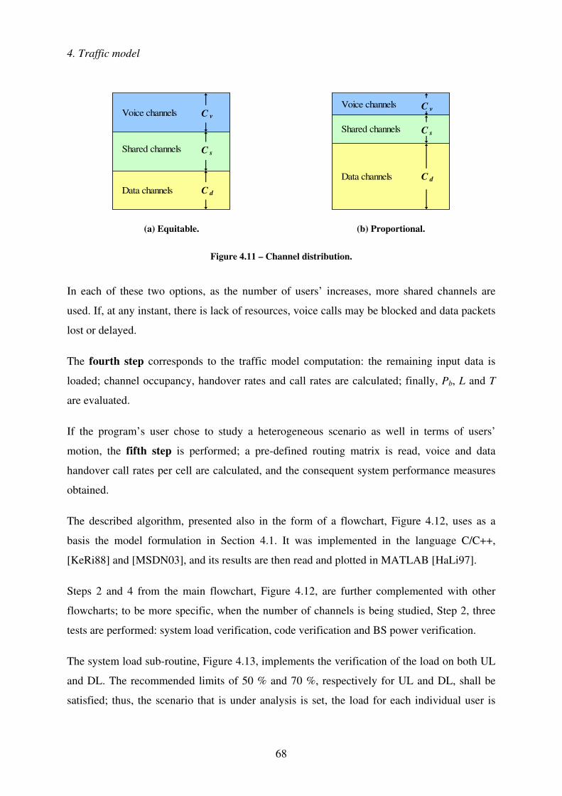
4. Traffic model
68
Voice channels
Shared channels
Data channels C d
C s
C v
Voice channels
Shared channels
Data channels C d
C s
C v
(a) Equitable. (b) Proportional.
Figure 4.11 – Channel distribution.
In each of these two options, as the number of users’ increases, more shared channels are
used. If, at any instant, there is lack of resources, voice calls may be blocked and data packets
lost or delayed.
The fourth step corresponds to the traffic model computation: the remaining input data is
loaded; channel occupancy, handover rates and call rates are calculated; finally, Pb, L and T
are evaluated.
If the program’s user chose to study a heterogeneous scenario as well in terms of users’
motion, the fifth step is performed; a pre-defined routing matrix is read, voice and data
handover call rates per cell are calculated, and the consequent system performance measures
obtained.
The described algorithm, presented also in the form of a flowchart, Figure 4.12, uses as a
basis the model formulation in Section 4.1. It was implemented in the language C/C++,
[KeRi88] and [MSDN03], and its results are then read and plotted in MATLAB [HaLi97].
Steps 2 and 4 from the main flowchart, Figure 4.12, are further complemented with other
flowcharts; to be more specific, when the number of channels is being studied, Step 2, three
tests are performed: system load verification, code verification and BS power verification.
The system load sub-routine, Figure 4.13, implements the verification of the load on both UL
and DL. The recommended limits of 50 % and 70 %, respectively for UL and DL, shall be
satisfied; thus, the scenario that is under analysis is set, the load for each individual user is

4. Traffic model
69
calculated and summed, and the thresholds are checked; in case any of these maximum
allowed limits is exceeded, a reduction on the number of DL codes is performed.
The code sub-routine, Figure 4.14, implements the verification of the number of codes
required to serve all users from the scenario under analysis; if the resulting value is below
256, no additional actions are undertaken; otherwise, the number of codes that is considered
corresponds to that threshold.
The BS power sub-routine, Figure 4.15, implements the verification of the power delivered by
the BS to the MTs. The first action required is the users’ distribution within the cell radius; for
that purpose, a pseudo-random function is called, and MTs are spread uniformly inside the
cell coverage area. The allowed propagation loss is calculated through (3.1); afterwards, the
BS power required to serve all users is summed and the results are compared with the
threshold as defined by the program’s user; again, if the required BS power is higher than the
one that was set up in the system, then an adjustment on the number of codes is performed.
Finally, the traffic model computation, Figure 4.16, is carried out. The missing input
parameters are read from input files prepared earlier, following the calculation of the
probability matrix; other parameters, like channel occupancy, HO rates and arrival rate, are in
the mean time computed as well. When all input parameters are known, one sole task
remains: the calculation of the three system behaviour parameters, namely, Pb, L and T.
Two particular scenarios are studied in Chapter 5, the corresponding results being presented
in Annexes C and D; in particular, the traffic model behaviour is first loaded with more voice
than data, and then an almost symmetrical scenario is analysed. Several considerations with
respect to the traffic model are drawn along the next chapter.

4. Traffic model
70
Start of UMTS scenarios analysis
Cell radius read from input parameters fileor calculated for a reference scenario
STEP 1
STEP 2
STEP 3
Calculation of the number of channels(C ≤ 128)
End of UMTS scenarios analysis
STEP 4
Traffic model computation (flowchart D)
Codesverification
(flowchart B)
TX BS powerverification
(flowchart C)
UL and DL system loadverification
(flowchart A)
STEP 5
Users' motion analysis fora heterogeneous scenario
Figure 4.12 – Traffic model algorithm, main flowchart.
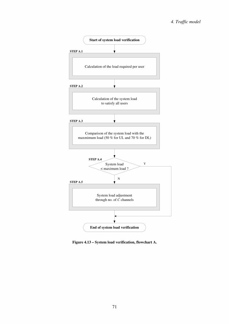
4. Traffic model
71
Start of system load verification
Calculation of the load required per user
STEP A.1
Calculation of the system loadto satisfy all users
STEP A.2
STEP A.3
Comparison of the system load with themaxmimum load (50 % for UL and 70 % for DL)
STEP A.5
System load adjustmentthrough no. of C channels
End of system load verification
System load< maximum load ?
STEP A.4
N
Y
Figure 4.13 – System load verification, flowchart A.
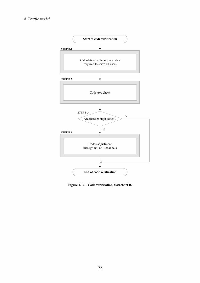
4. Traffic model
72
Calculation of the no. of codesrequired to serve all users
Start of code verification
Code tree check
STEP B.2
STEP B.4
Codes adjustmentthrough no. of C channels
End of code verification
Are there enough codes ?
STEP B.3
N
Y
STEP B.1
Figure 4.14 – Code verification, flowchart B.
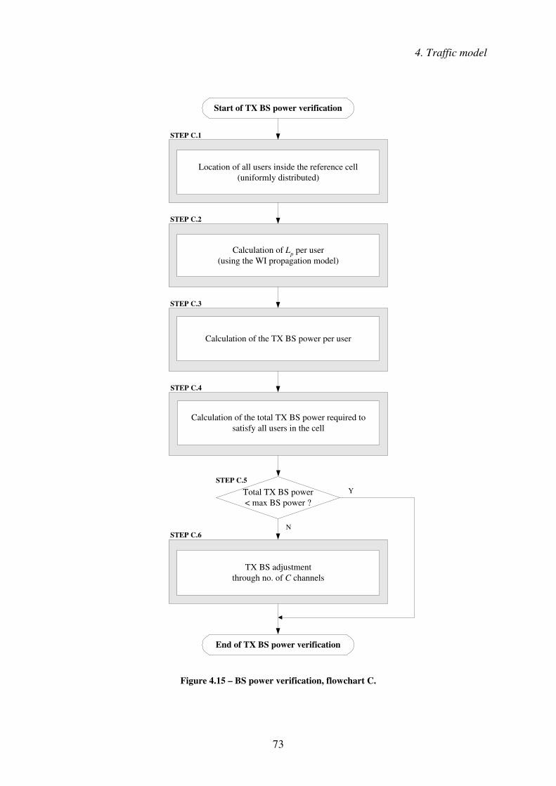
4. Traffic model
73
Start of TX BS power verification
Location of all users inside the reference cell(uniformly distributed)
STEP C.1
Calculation of Lp per user(using the WI propagation model)
STEP C.2
STEP C.3
Calculation of the TX BS power per user
STEP C.6
TX BS adjustmentthrough no. of C channels
End of TX BS power verification
Total TX BS power< max BS power ?
STEP C.5
N
Y
STEP C.4
Calculation of the total TX BS power required tosatisfy all users in the cell
Figure 4.15 – BS power verification, flowchart C.

4. Traffic model
74
Start of traffic model computation
Loading all input pars.(λv
n, λdn, 1/µv, 1/µd, R,
1/ηv, 1/ηd, C, Cv, Cd, B)
Calculation of thesteady state prob.
(pij and pij')
Calculation of the voicechannel occupancy time
(µcv)
Calculation of the datachannel occupancy time
(µcd)
STEP D.0
STEP D.1
Calculation of the voicecall handover rate
(λvh)
Calculation of the datacall handover rate
(λdh)
STEP D.2
STEP D.3
Calculation of the voicecall arrival rate
(λv)
Calculation of the datacall arrival rate
(λd)
STEP D.4
Estimation of the voiceblocking probability
(Pb)
Estimation of the dataloss probability
(L)
Estimation of the meandelay data
(Τ )
End of traffic model computation
STEP D.5
Figure 4.16 – Traffic model computation, flowchart D.

75
5 Analysis of results
5.1 Description of scenarios under study
Two different scenarios are analysed in this chapter, Table 5.1: one that weighs mainly a
considerable amount of voice users and scarce data users, Scenario A, and another where the
system load due to voice users is not as predominant as the one due to data users, Scenario B.
Table 5.1 – Number of users forming Scenarios A and B.
Scenario A Scenario B UL DL UL DL
Speech 80 80 10 10
VideoT 10 10 2 2
StrMMLQ 0 0 2 2
StrMMHQ 0 0 2 2
WWW 1 1 5 5
LocBas 1 1 2 2
MMS 2 0 5 0
Email 0 2 0 5
FDwnld 1 1 5 5
The traffic model is run for the number and type of users as specified, aiming at analysing the
system performance in terms of voice call blocking probability, Pb, data loss probability, L,
and mean data delay, T. The output of the model is provided as a function of the user’s
motion, between 0 and 120 km/h, and as a function of the buffer size, up to 20 MB. When the
users’ speed is under analysis, two different buffer sizes will be used: 20 MB and half of it,
10 MB; on the other hand, when the buffer size is the object of analysis, two different users’
speeds are set: 15 km/h and 60 km/h.
Other parameters will be set to different input values at the start of the program, in order to
study further the performance of the traffic model, e.g., the cell radii and the channel
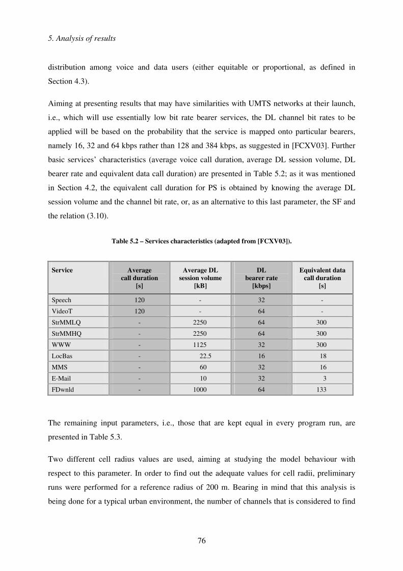
5. Analysis of results
76
distribution among voice and data users (either equitable or proportional, as defined in
Section 4.3).
Aiming at presenting results that may have similarities with UMTS networks at their launch,
i.e., which will use essentially low bit rate bearer services, the DL channel bit rates to be
applied will be based on the probability that the service is mapped onto particular bearers,
namely 16, 32 and 64 kbps rather than 128 and 384 kbps, as suggested in [FCXV03]. Further
basic services’ characteristics (average voice call duration, average DL session volume, DL
bearer rate and equivalent data call duration) are presented in Table 5.2; as it was mentioned
in Section 4.2, the equivalent call duration for PS is obtained by knowing the average DL
session volume and the channel bit rate, or, as an alternative to this last parameter, the SF and
the relation (3.10).
Table 5.2 – Services characteristics (adapted from [FCXV03]).
Service Average call duration
[s]
Average DL session volume
[kB]
DL bearer rate
[kbps]
Equivalent data call duration
[s]
Speech 120 - 32 -
VideoT 120 - 64 -
StrMMLQ - 2250 64 300
StrMMHQ - 2250 64 300
WWW - 1125 32 300
LocBas - 22.5 16 18
MMS - 60 32 16
E-Mail - 10 32 3
FDwnld - 1000 64 133
The remaining input parameters, i.e., those that are kept equal in every program run, are
presented in Table 5.3.
Two different cell radius values are used, aiming at studying the model behaviour with
respect to this parameter. In order to find out the adequate values for cell radii, preliminary
runs were performed for a reference radius of 200 m. Bearing in mind that this analysis is
being done for a typical urban environment, the number of channels that is considered to find

5. Analysis of results
77
the appropriate cell radius corresponds to those obtained for an average users’ motion of
30 km/h, Table 5.4.
Table 5.3 – Input parameters common to Scenarios A and B.
Parameters Values
DL codes 256
BS transmitted power [dBm] 43
Maximum UL load [%] 50
Maximum DL load [%] 70
Maximum buffer size [MB] 20
λv100 [calls/s] 0.015
λd100 [calls/s] 0.01
Table 5.4 – No. of codes for R = 200 m at 30 km/h, Scenarios A and B.
Equitable distribution Proportional distribution
Scenario A ττττv = 120 s and ττττd = 69.9 s
Total 63 63
Voice 21 47
Data 21 16
Shared 21 0
Scenario B ττττv = 120 s and ττττd = 134.5 s
Total 59 59
Voice 19 13
Data 19 46
Shared 21 0
With the number of codes, the call rates and corresponding average duration, it is possible to
define the cell radius values more accurately, as specified earlier in Section 4.2; the range of
possible values is shown in Figure 5.1. Considering Scenario A, for an equitable distribution
of channels, the cell radius may reach 300 m for voice and 400 m for data (red line); for a
proportional distribution of channels, voice goes beyond 450 m (blue line), but data only
allows a maximum of 350 m radius (green line). For Scenario B, the equitable distribution of
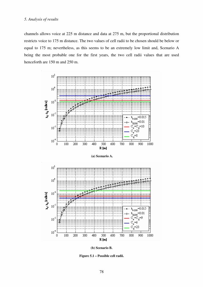
5. Analysis of results
78
channels allows voice at 225 m distance and data at 275 m, but the proportional distribution
restricts voice to 175 m distance. The two values of cell radii to be chosen should be below or
equal to 175 m; nevertheless, as this seems to be an extremely low limit and, Scenario A
being the most probable one for the first years, the two cell radii values that are used
henceforth are 150 m and 250 m.
(a) Scenario A.
(b) Scenario B.
Figure 5.1 – Possible cell radii.

5. Analysis of results
79
5.2 Analysis of the number of channels
The number of codes obtained by simulating Scenarios A and B, for both 150 and 250 m cell
radius, are presented in Figure 5.2 and Figure 5.3, respectively.
(a) Equitable distribution of channels. (b) Proportional distribution of channels.
Figure 5.2 – Number of codes for Scenario A.
For Scenario A, the proportional distribution of channels, Figure 5.2 (b), shows that the
majority of the available codes are devoted to voice users. On the other hand, it can be seen
that in Figure 5.3 (b) the most important bandwidth will be provided to data users, those who
are loading the system more. The proportional distribution of channels reflects better the real
load of each service type, leading, as it will be seen later, to a better overall system
performance than the equitable distribution.
Another additional comment arises concerning Figure 5.2 and Figure 5.3: as the users’ speed
increases, it is possible to observe that the number of channels provided by the system gets
smaller. It is seen in Section 4.2 that the overall channels vary as a function of many factors:
the system load on both UL and DL, the BS transmitted power and the number of DL codes;
these parameters are dependent as well on other variables (e.g., Eb/N0, bit rate, orthogonal
factor, losses, gains and other margins). The global tendency of the system results,

5. Analysis of results
80
considering all these varying parameters, corresponds to a decrease on the number of channels
with a growing average users’ speed.
(a) Equitable distribution of channels. (b) Proportional distribution of channels.
Figure 5.3 – Number of codes for Scenario B.
It has to be pointed out that, when applying radii of 150 and 250 m, the same numbers of
codes as those shown in Figure 5.2 and Figure 5.3 are obtained for the corresponding
scenarios; this is basically due to the fact that the system is exceeding the allowed load limits,
50 % on UL and 70 % on DL, whereas the BS power required to satisfy all users does not go
beyond the limit of 43 dBm; if the BS transmitted power would correspond to the most severe
limiting system factor, and as it depends on the position of the MTs with respect to the BS,
the number of channels for two cells with different sizes would be distinct.
The channels in UMTS are not equally sized: the number of codes required per service, which
is a direct result of the DL SFs, which, in turn, depends on the channel bit rates, will
determine the size and quantity of the UMTS channels; considering a real scenario, with
different users / services popping up, the instantaneous number of channels may present a
discontinuous variation.
5. Analysis of results
81
5.3 Comparison of traffic model results with known models
There are essentially two ways to validate the traffic model results: either by looking into real
data and comparing it with the model output, or to use well known traffic models that may,
for particular situations, represent accurately the reality. The level of development of network
elements and terminals, achieved up to date, does not allow following either one or the other
suggested approaches, per se, as they are not enough to test and certify the accuracy of the
present traffic model.
There are currently very few UMTS networks in operation around the world; moreover, the
amount of UMTS terminals already in the market is so small and their prices are still so high,
that the current users do not yet represent on average the overall population and its behaviour;
thus, the analysis of real data needs to be postponed for a later point in time, when some
actual and reliable UMTS traffic information is made available.
As far as the comparison of known traffic models against the present one is concerned, it is
also not a straightforward task. There are currently no models that allow simultaneously
multi-service traffic, thus, with diverse characteristics. Consequently, it was decided to
separate voice from data and compare only the voice call blocking probabilities obtained with
the results of the Erlang-B model; due to the UMTS characteristics embedded in the model,
e.g., the variable number of channels as a function of instantaneous environment conditions, it
is not expected that the traffic model results match completely the Erlang-B ones. With
respect to data services, and as none of the known models present similarities with the nature
of the traffic model under analysis, no comparison in terms of data losses and delays aiming
at validating the traffic model behaviour for data is possible.
As said in Chapter 3, the Erlang-B model does not have capability to store any call that cannot
be served due to lack of resources, meaning that users willing to enter the system while there
are no available channels are simply lost (blocked calls are cleared); this is basically what
happens with voice users emulated through the traffic model, as no buffering for this kind of
calls is foreseen.
The blocking probability for an Erlang-B model is given by (3.25), and, by varying the
amount of traffic, A, between 1 and 100 Erlang, for systems with, e.g., 8, 16, 32 or 64 voice

5. Analysis of results
82
channels, is given by Figure 5.4. When the number of channels becomes smaller, it is visible
that the blocking probabilities, for the same amount of traffic, increase.
Figure 5.4 – Blocking probability for Erlang-B model.
To obtain the exact number of voice channels, Cv, for each scenario under analysis, the first
block of the traffic model algorithm is implemented (steps 0 to 3, as specified in Chapter 4);
the resulting values are plotted in Figure 5.5; these will be used in the Erlang-B model to
calculate the traffic.
It should be pointed out that the call rates used for Scenarios A and B, for the purpose of
comparing the traffic model results with other known traffic models, correspond to the ones
obtained by considering a 250 m cell radius; both new and HO calls are accounted for.
The blocking probabilities, obtained through the traffic model, Figure 5.6, and the Erlang-B
model, Figure 5.7 and Figure 5.8, are plotted for users’ speeds of 30, 60, 90 and 120 km/h.
Scenario A being a predominant voice users’ scenario, and, knowing that voice does not load
extremely the system, the model does not lead to reflect any probability of blocking, i.e., it is
below 10-2 %. With respect to Scenario B it is the other way around, as there is much more

5. Analysis of results
83
load due to data than voice calls, especially for the proportional distribution of resources;
while the number of channels for voice users decreases, it imposes an increase on the
blocking probability when obtained through the current traffic model; this is visible in
Figure 5.6 for the proportional distribution of channels, where few resources are left for voice;
with respect to the equitable distribution of channels, and, as can be seen, only for very high
average speeds, e.g., 120 km/h, a blocking probability greater than 10-2 % is experienced.
(a) Scenario A. (b) Scenario B.
Figure 5.5 – Available voice channels versus users’ speed.
A clarification needs to be done with respect to the Erlang-B calculations, to perform the
comparison with the traffic model: the speeds for which the models’ results are to be
compared (the ones mentioned earlier), are converted into a specific number of channels,
plotted in Figure 5.5; those numbers of channels are used to obtain the amount of traffic
through (3.17); afterwards, by applying the Erlang-B model, one obtains the corresponding
blocking probabilities. Figure 5.7 and Figure 5.8 show the resulting Pb for Scenarios A and B.
It is possible to observe in Figure 5.7 (a) and Figure 5.8 (a) that the results for the equitable
distributions from the two scenarios are similar, as a consequence of the number of voice
channels, which is almost equal, Figure 5.5.

5. Analysis of results
84
Figure 5.6 – Traffic model blocking probability for Scenario B.
Another aspect that should be noted is the fact that in Figure 5.7 (a) and in Figure 5.8 (a) and
(b), there are some overlapped curves; this happens when the number of channels does not
change for different users’ speeds, Figure 5.5, leading the corresponding blocking probability
curves, obtained through the Erlang-B model, to be overlapped.
It becomes clear from Figure 5.6, Figure 5.7 and Figure 5.8 that, for the same amount of
channels, the Erlang-B model presents higher blocking probabilities than the traffic model
under analysis, being the attained values rather significant, not negligible. Additionally, it is
possible to note that, when the system delivers relatively few channels for voice, the two
models present very similar results: the curves for the proportional distribution of channels in
Figure 5.6 and Figure 5.8 (b) show visibly this analogous behaviour; in contrary, when the
amount of voice channels increases, the results from the two traffic models no longer agree,
the Erlang-B model showing, as known, to be a conservative traffic model.
It has to be mentioned that all the modifications required to adapt the model of [HaLH00] to a
UMTS network model, as detailed in Section 4.2, made it rather complex; quite many security
margins were introduced all over the planning steps (e.g., Mlog-normal, Mfast-fading, ηUL, ηDL, and
others), while defining parameters and calculating partial results; it is clear that the model
needs further refining, after real data is available, to tune it into a realistic and trustful model.
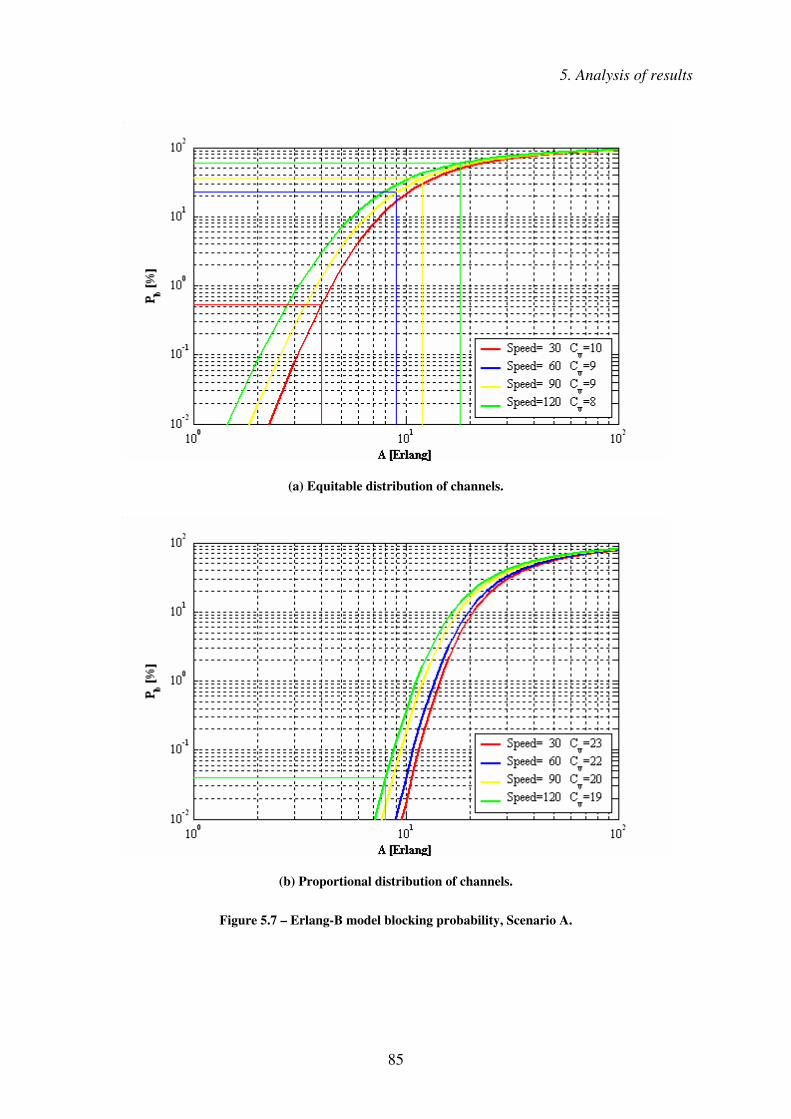
5. Analysis of results
85
(a) Equitable distribution of channels.
(b) Proportional distribution of channels.
Figure 5.7 – Erlang-B model blocking probability, Scenario A.
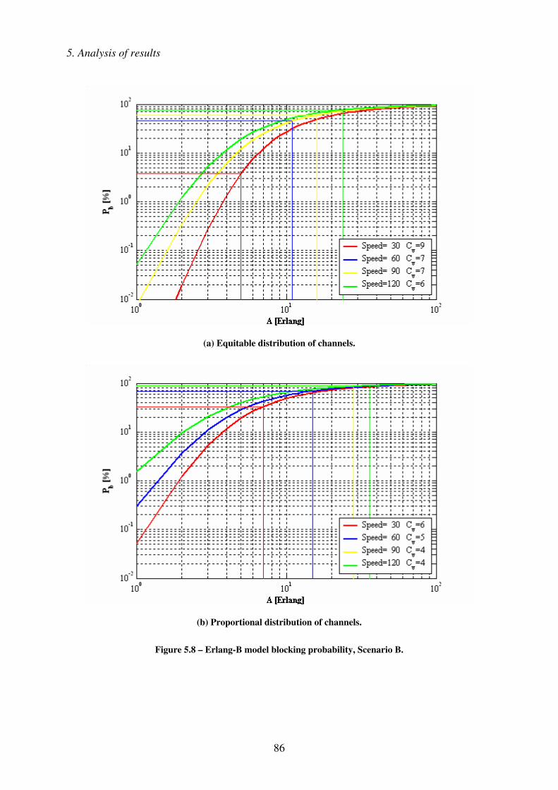
5. Analysis of results
86
(a) Equitable distribution of channels.
(b) Proportional distribution of channels.
Figure 5.8 – Erlang-B model blocking probability, Scenario B.
5. Analysis of results
87
5.4 Results for a single cell
Voice and data call rates, λv and λd, obtained by knowing the effective cell radius and the
reference rates listed in Table 5.3, together with the (equivalent) average call duration
considered in Table 5.2, τv and τd, and weighed against the number of users, fix the amount of
traffic in the system. The model is forced to support a specific amount of traffic,
[(τv, τd), (λv, λd)], and two times that quantity, [(2τv, 2τd), (λv, λd)] or [(τv, τd), (2λv, 2λd)].
Before going into a more detailed analysis of the traffic model results, it is worthwhile to
provide an explanation on the behaviour of the three parameters that are under discussion:
voice call blocking probability, Pb, data loss probability, L, the mean data delay, T.
According to the principles of the traffic model, Pb is calculated through (4.5), meaning that
its resulting value corresponds to the sum of a number of pij elements, and depends on the
number of channels available. If the condition Cv ≤ C-Cd-1 is satisfied, those pij fall inside
some red delimiters as drawn in Figure 5.9 (a) (e.g., when the total amount of channels is
equitably distributed between voice and data users); otherwise, these boundaries may be
represented as in Figure 5.10 (a) and Figure 5.11 (a) (e.g., when the available channels are
proportionally distributed to the users that compose the scenario under analysis; in case there
are more voice users than data, Figure 5.10 applies; for more data users, Figure 5.11 is a
better illustration of the situation). It is clear from those figures that Pb is smaller when there
are a large number of channels devoted to voice users; if, contrariwise, there are very few
voice channels, the Pb influence area gets more extended and further voice calls get blocked.
L is also dependent on pij, and on the size of the buffer, B; the data loss probability is, for the
purpose of the current traffic model, obtained through (4.7). Similarly to Pb, L does have an
influence area as well, graphically delimited through the green frames from Figure 5.9 (a),
Figure 5.10 (a) and Figure 5.11 (a). Undoubtedly, the greater the number of data channels, Cd,
and B, the smaller the area inside the green borders; consequently, L decreases. If either the
buffer is small or the data channels are reduced, that same influence area increases and more
packets may get lost.

5. Analysis of results
88
(a) pij matrix.
(b) pij’ matrix.
Figure 5.9 – Equitable distribution of channels.

5. Analysis of results
89
(a) pij matrix.
(b) pij’ matrix.
Figure 5.10 – Proportional distribution of channels, predominant voice users.

5. Analysis of results
90
(a) pij matrix.
(b) pij’ matrix.
Figure 5.11 – Proportional distribution of channels, predominant data users.
5. Analysis of results
91
Finally, the tendency of the last system parameter, the mean data delay, shall be analysed.
From (4.9), a non-straightforward behaviour of T is to be expected: there are three variables
that influence the final result, namely, the differentiation of the probability matrix pij,
hereafter referred to as pij’ matrix, the data call rates, λdn and λd
h, and the data loss probability,
L. The pij’ influence area is shown in Figure 5.9 (b), Figure 5.10 (b) and Figure 5.11 (b), for
the distribution of channels mentioned earlier; it becomes visible from those figures that the
number of pij’ elements that contribute to T is higher when data channels are reduced. T varies
inversely with the data call rates (new and handover), and, as it was already referred earlier,
there is a straightforward connection between cell radius and data call rates, as well as users’
speed and handover call rates; considering simply the aspects that affect data call rates,
another conclusion is reached: T decreases for higher radii and for higher users’ speeds. The
third aspect that influences T is L: as L rises, T tends to follow that behaviour. These three
aspects assume, for specific values, rather different weighs: one or the other becomes
predominant or irrelevant, depending on the various inputs that are being given to the traffic
model, instead of assuming a clear tendency.
The complete results of the traffic model behaviour for Scenarios A and B is presented in
Annexes C and D, respectively. Some important and determinant aspects are nevertheless
addressed in what follows.
The traffic model is forced to react to the variation of four basic system parameters:
− average speed at which users’ move around;
− cell radius for which the analysis is being performed;
− buffer size;
− channels’ distribution between voice and data users.
As expected, the average speed at which users move around influences decisively the results
of the traffic model. A first aspect that justifies this comment is the number of channels
supported by the system when users’ speed varies; when adapting the traffic model under
analysis to UMTS (Section 4.2), the number of channels is made dependent on three system
aspects: UL/DL loads, BS transmission power and available DL codes. UL/DL loads, as well
as the BS transmission power, depend, among others, on Eb/N0 values, which are strictly

5. Analysis of results
92
connected to the users’ speed. A reduction on the amount of channels made available by the
system with an increase on the users’ speed is clearly visible in Figure 5.2 or Figure 5.3, as
well as on the complete sets of results presented in Annexes C and D.
When there is a reduction on the number of channels with speed increase, the voice call
blocking probability will be affected: the top limit of the Pb influence area (red borders) gets
closer to the beginning of the probability matrix and more pij elements are thus summed up.
Figure 5.12 shows clearly this tendency, especially for higher traffic values,
[(2τv, 2τd), (λv, λd)] or [(τv, τd), (2λv, 2λd)]; the input data corresponds to Scenario B with a
cell radius of 250 m, a 20 MB buffer size and channels distributed equitably among users.
Figure 5.12 – Blocking probability as a function of users’ speed.
Both the green and the red curves are overlapped in Figure 5.12; this results directly from the
fact that when either the call duration or the call rates are doubled, the consequence is the
same and corresponds to doubling the amount of traffic in the system. The blocking
probabilities for [(τv, τd), (λv, λd)] are, for any speed up to 120 km/h, kept at a rather
negligible value; in contrary, when the amount of traffic in the system doubles, the blocking
probabilities assume, for average speeds higher than 60 km/h, values above 2 %, beyond the
acceptable threshold commonly used in GSM.

5. Analysis of results
93
With respect to L, and considering solely the channel number aspect (the buffer effect will be
analysed later on), it can be said that reducing channels in general means approximating the
bottom limit of the L influence area (green boundary) to the beginning of the probability
matrix; clearly, less pij elements will count for L when users’ speed is increased, Figure 5.13.
Figure 5.13 – Data loss probability as a function of users’ speed.
These results were obtained for Scenario B, considering a cell with 250 m radius, 20 MB of
buffering capability and channels distributed proportionally among voice and data.
It is visible in Figure 5.13 that the red and the green curves are overlapped, due again to the
fact that the pij matrices coincide for these two situations. For lower traffic amounts, e.g., the
blue curve, the effect of an increase on speed is smoother than for higher traffic values; the pij
influence area is, in this case, more distant from the green borders, meaning that an increase
on the users’ speed does not push straight away the relevant pij elements out of the boundaries
that determine L, as is the case when the amount of traffic in the system is high.
Increasing users’ speed means, thus, less channels and the pij’ influence area decreases as
well; the overall data call rates also augment with speed; finally, as mentioned earlier, L gets
smaller with higher speeds, leading to a decrease of T. These three variables will altogether
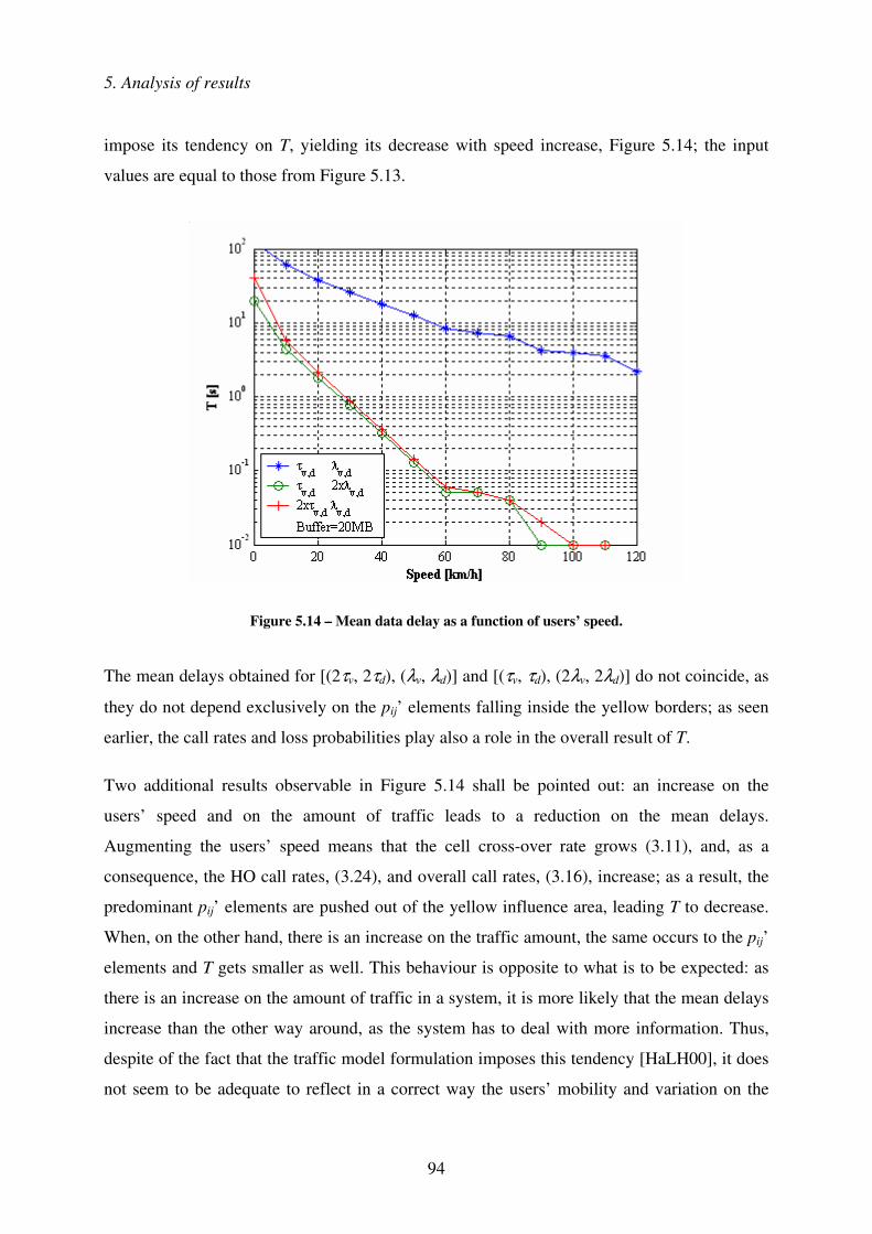
5. Analysis of results
94
impose its tendency on T, yielding its decrease with speed increase, Figure 5.14; the input
values are equal to those from Figure 5.13.
Figure 5.14 – Mean data delay as a function of users’ speed.
The mean delays obtained for [(2τv, 2τd), (λv, λd)] and [(τv, τd), (2λv, 2λd)] do not coincide, as
they do not depend exclusively on the pij’ elements falling inside the yellow borders; as seen
earlier, the call rates and loss probabilities play also a role in the overall result of T.
Two additional results observable in Figure 5.14 shall be pointed out: an increase on the
users’ speed and on the amount of traffic leads to a reduction on the mean delays.
Augmenting the users’ speed means that the cell cross-over rate grows (3.11), and, as a
consequence, the HO call rates, (3.24), and overall call rates, (3.16), increase; as a result, the
predominant pij’ elements are pushed out of the yellow influence area, leading T to decrease.
When, on the other hand, there is an increase on the traffic amount, the same occurs to the pij’
elements and T gets smaller as well. This behaviour is opposite to what is to be expected: as
there is an increase on the amount of traffic in a system, it is more likely that the mean delays
increase than the other way around, as the system has to deal with more information. Thus,
despite of the fact that the traffic model formulation imposes this tendency [HaLH00], it does
not seem to be adequate to reflect in a correct way the users’ mobility and variation on the

5. Analysis of results
95
traffic amount. It is important to refer that this is a point where a tuning of the model is clearly
required, to correct this abnormal behaviour with respect to the data packet mean delays.
When forcing the traffic model to react to the variation of the cell radius, further conclusions
are reached. When augmenting the cell radius, the call rates increase and, consequently, the
predominant pij elements may slightly shift to the centre of the probability matrix. The red
delimiters, influencing Pb, encompass more matrix elements; for this particular buffer size,
the pij elements falling inside the green borders turn also to be higher; thus, the voice blocking
and the data loss probabilities grow, Figure 5.15 and Figure 5.16. In contrast, the yellow
borders, which are not influenced directly by the buffer size, contain less predominant pij’
elements and T could decrease; on the other hand, as L grows, T may as well rise up; finally,
increasing the call rates leads T to get reduced; the final tendency of T is not very
straightforward, but results from weighing these three components and identifying which
one(s) impose its behaviour at each instant.
(a) Blocking call probability. (b) Data loss probability.
Figure 5.15 – Pb and L as a function of the users’ speed, for R = 100 m.
Figure 5.15 and Figure 5.16 result from running the traffic model for Scenario B with a
10 MB buffer, considering a proportional distribution of channels, and the cell radius being
set to 100 and 200 m, respectively.

5. Analysis of results
96
(a) Blocking call probability. (b) Data loss probability.
Figure 5.16 – Pb and L as a function of the users’ speed, for R = 200 m.
It has to be pointed out that for a 10 MB buffer and a 100 m radius, Figure 5.15 (b), the data
loss probabilities assume rather very small values, for the scenario under analysis: for high
traffic, it only reaches 10-2 % and the users’ speed does even not influence L.
There are two tendencies that may additionally be observed in Figure 5.15 and Figure 5.16:
first, when increasing the users’ speed, Pb increases and L gets stationary or decreases, as seen
earlier; the second aspect is the fact that, when augmenting the cell radius, Pb keeps that
tendency to increase with speed, whereas L tends to decrease; this tendency of L is especially
verified for high traffic, [(2τv, 2τd), (λv, λd)] or [(τv, τd), (2λv, 2λd)]; the reason for this
behaviour is the fact that the pij influencing area is initially outside the green borders, i.e., for
small radii or low traffic, and then, it enters the L influence area and, finally, starts going
beyond the limits for higher traffic values.
If, in addition, it happens that the increase on the cell radius leads the system to get limited by
the BS transmitted power, then a reduction on the number of channels is to be expected in
conjunction to the extension of the cell radius. Thus, its effect will affect, in a cumulative
form, the system parameters.
5. Analysis of results
97
Analysing now what happens to the results of the traffic model when the buffer size, B, is
changed, it is possible to conclude, as expected, that voice calls are neither positively, nor
negatively, affected by that system element. Contrariwise, L is directly influenced by the size
of the buffer: as seen in Figure 5.9 (a), Figure 5.10 (a) and Figure 5.11 (a), one of the
quadrilateral sides of the green shape is formed by B, leading to the conclusion that the
greater the buffer is the smaller L gets; as a consequence, T tends to decrease.
The fourth system parameter that requires to be analysed is the channels’ distribution between
voice and data users: it is definitively one of the parameters that influences most the
behaviour of the traffic model. The equitable distribution of channels between voice and data
users, keeping the remaining channels as spare for any user type, brings more disadvantages
to the majority of the users when the system becomes heavily loaded; the proportional
distribution of channels between voice and data users, as a function of the scenario under
analysis, seems to be a more realistic approach and, without any doubt, more fair for the
majority of users. When a scenario with many voice users is under analysis, like Scenario A,
the equitable distribution of channels will benefit data users, as they receive, a priori, more
than one third of the resources; on the other hand, when talking about a scenario that
encompasses fundamentally data users, Scenario B, the equitable distribution of channels
favours a little the voice users, making the blocking probability much smaller due to a
“possible” over-dimension of the number of channels kept for voice.
The major conclusions related to the system behaviour are summarised in Table 5.5.
Looking into the complete results of Scenarios A and B, presented in Annexes C and D,
respectively, the expected tendencies of Pb, L and T, are confirmed: the results agree ipso
facto with the summary presented in Table 5.5.
There are, nevertheless, aspects on the performance of the traffic model that may be analysed
and, why not, turned into points to be further enhanced; some comments on this direction are
presented in the last chapter.
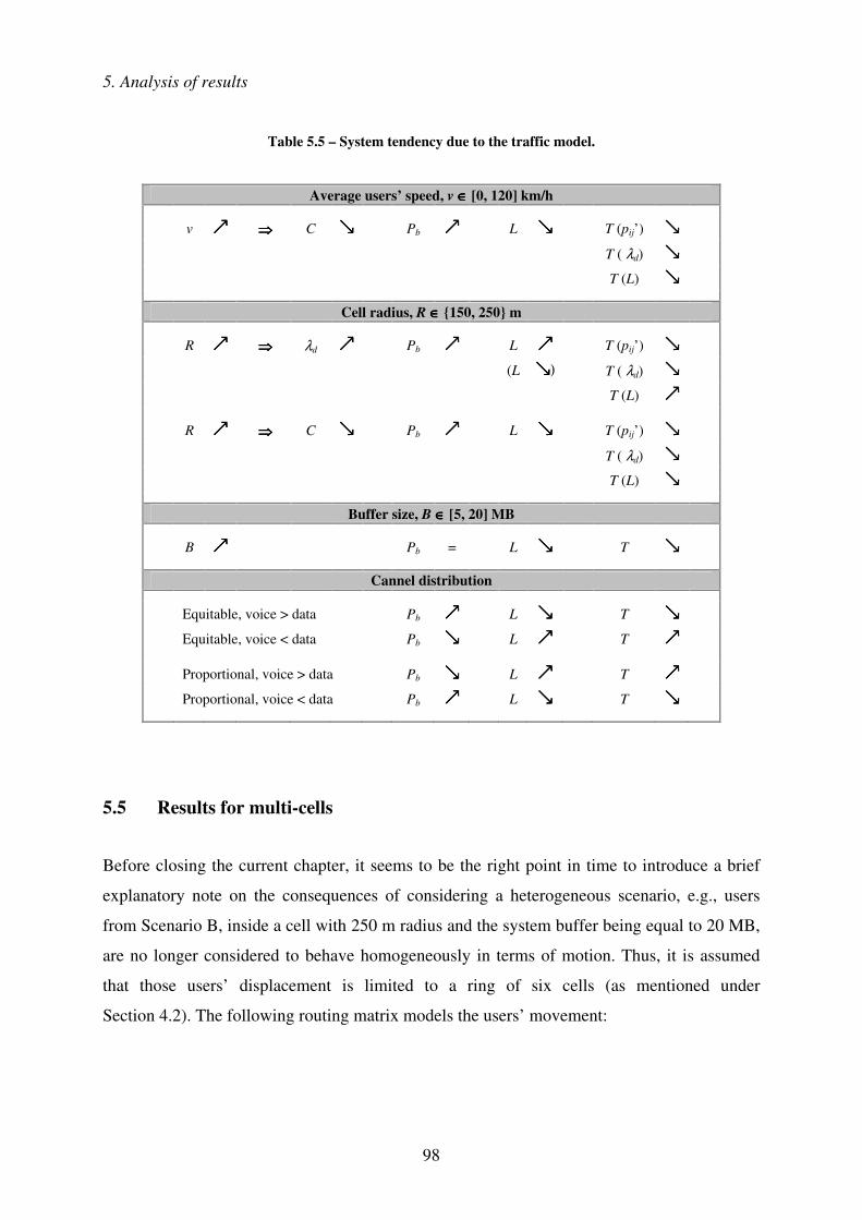
5. Analysis of results
98
Table 5.5 – System tendency due to the traffic model.
Average users’ speed, v ∈∈∈∈ [0, 120] km/h
v ���� ���� C ���� Pb ���� L ���� T (pij’) ����
T ( λd) ����
T (L) ����
Cell radius, R ∈∈∈∈ {150, 250} m
R ���� ���� λd ���� Pb ���� L ���� T (pij’) ����
(L ����) T ( λd) ����
T (L) ����
R ���� ���� C ���� Pb ���� L ���� T (pij’) ����
T ( λd) ����
T (L) ����
Buffer size, B ∈∈∈∈ [5, 20] MB
B ���� Pb = L ���� T ����
Cannel distribution
Equitable, voice > data Pb ���� L ���� T ����
Equitable, voice < data Pb ���� L ���� T ����
Proportional, voice > data Pb ���� L ���� T ����
Proportional, voice < data Pb ���� L ���� T ����
5.5 Results for multi-cells
Before closing the current chapter, it seems to be the right point in time to introduce a brief
explanatory note on the consequences of considering a heterogeneous scenario, e.g., users
from Scenario B, inside a cell with 250 m radius and the system buffer being equal to 20 MB,
are no longer considered to behave homogeneously in terms of motion. Thus, it is assumed
that those users’ displacement is limited to a ring of six cells (as mentioned under
Section 4.2). The following routing matrix models the users’ movement:
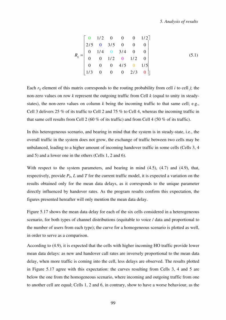
5. Analysis of results
99
1/ 2 0 0 0 1/ 22 / 5 3/ 5 0 0 0
0 1/ 4 3/ 4 0 00 0 1/ 2 1/ 2 00 0 0 4 / 5 1/ 5
1/ 3 0 0 0
0
02 /
0
0
00
3
ijR
� � �� �� �
= � �� �� �� �� � �
(5.1)
Each rij element of this matrix corresponds to the routing probability from cell i to cell j; the
non-zero values on row k represent the outgoing traffic from Cell k (equal to unity in steady-
states), the non-zero values on column k being the incoming traffic to that same cell; e.g.,
Cell 3 delivers 25 % of its traffic to Cell 2 and 75 % to Cell 4, whereas the incoming traffic in
that same cell results from Cell 2 (60 % of its traffic) and from Cell 4 (50 % of its traffic).
In this heterogeneous scenario, and bearing in mind that the system is in steady-state, i.e., the
overall traffic in the system does not grow, the exchange of traffic between two cells may be
unbalanced, leading to a higher amount of incoming handover traffic in some cells (Cells 3, 4
and 5) and a lower one in the others (Cells 1, 2 and 6).
With respect to the system parameters, and bearing in mind (4.5), (4.7) and (4.9), that,
respectively, provide Pb, L and T for the current traffic model, it is expected a variation on the
results obtained only for the mean data delays, as it corresponds to the unique parameter
directly influenced by handover rates. As the program results confirm this expectation, the
figures presented hereafter will only mention the mean data delay.
Figure 5.17 shows the mean data delay for each of the six cells considered in a heterogeneous
scenario, for both types of channel distributions (equitable to voice / data and proportional to
the number of users from each type); the curve for a homogeneous scenario is plotted as well,
in order to serve as a comparison.
According to (4.9), it is expected that the cells with higher incoming HO traffic provide lower
mean data delays: as new and handover call rates are inversely proportional to the mean data
delay, when more traffic is coming into the cell, less delays are observed. The results plotted
in Figure 5.17 agree with this expectation: the curves resulting from Cells 3, 4 and 5 are
below the one from the homogeneous scenario, where incoming and outgoing traffic from one
to another cell are equal; Cells 1, 2 and 6, in contrary, show to have a worse behaviour, as the

5. Analysis of results
100
mean delays are higher than the obtained for the homogeneous scenario; Cell 4 presents the
highest handover rate and Cell 6 the lowest one (5.1), and, through Figure 5.17, those
correspond to the cells that encompass less and more delays, respectively.
(a) Equitable distribution of channels.
(b) Proportional distribution of channels.
Figure 5.17 – Mean data delay vs. speed for a heterogeneous scenario.

5. Analysis of results
101
The homogeneous curve equals the one presented in Figure D.3 as expected, as the input
parameters are the same.
When setting now three different speed values, namely, 10, 20 and 30 km/h, the
corresponding delays are shown for each cell in Figure 5.18.
(a) Equitable distribution of channels.
(b) Proportional distribution of channels.
Figure 5.18 – Mean data delay per cell for a heterogeneous scenario.

5. Analysis of results
102
It is clearly observed through Figure 5.18 that an increase on speed leads, for every cell, to a
decrease on the corresponding delays. Additionally, when comparing the cells among each
others, it is possible to remark which ones have more / less incomer users, according to the
lower / higher delays presented. Finally, it should be noted that for the equitable distribution
of channels, the delays are greater than the proportional distribution (for the scenario under
analysis, which takes into consideration more load due to data users rather than voice); as
seen earlier, this behaviour is justified by the number of channels that each of these
distributions allocates to voice / data users.

103
6 Conclusions
This thesis presents a traffic model that considers scenarios with voice and data users, mixing
up, in the same infrastructure, different services and applications. Many UMTS aspects are
built in the model, so that the performance of a UMTS network, in terms of voice call
blocking probabilities, data loss probabilities and mean data delays, is estimated.
The large amount of parameters that need to be addressed and the many environments that can
be visited by a 3G user, turn the task of gathering all details into a single traffic model rather
difficult to achieve. As a consequence, some simplifications had to be proposed and
implemented in the model, aiming at reducing its complexity.
The traffic model that was studied, like any other models, e.g., Erlang-B or Engset models,
has a limited scope of applicability. It is referred, along the previous chapters, the
simplifications that are done in order to allow the use of this model to study the traffic
behaviour of a UMTS network; some of the simplifications challenge the accuracy of the
model a little bit, as the particularities of the scenarios, service characteristics, etc., get
smoother or lost with all the simplifications done; nevertheless, the results achieved are in line
with the original expectations. Some comments in terms of the results obtained through this
traffic model may thus be drawn.
The total amount of channels that, at any time, the system is making available to the users,
keeping in mind that the traffic model is analysing the behaviour of a number of users under
the coverage of one BS, corresponds to the most critical aspect in UMTS. Rather few
simultaneous users may be served if one considers the number of codes that need to be
employed per user and per service; however, it has to be said that all the results were obtained
using one single carrier frequency, and that, e.g., in Portugal, 3G mobile operators were
awarded 4 carriers in FDD mode; when more traffic is to be expected, one or two carriers can
additionally be put on service per BS, although care has to be taken in order to control any
interference that may occur. The low number of channels is due to the fact that many security
margins are considered when performing the various steps that precede the calculation of the
number of channels; the majority of the tested scenarios showed that the system is limited by
6. Conclusions
104
the DL load (the way the traffic model is handling interference). As long as real data cannot
be measured, any tunings may be useless.
When analysing the two ways of distributing channels between voice and data users, it
becomes clear from the results that allocating channels on a proportional form is better for the
majority of users than distributing them equitably between voice and data users. If, in
addition, the interoperability between networks becomes effective, some calls may be served
by other networks that provide overlapped coverage, e.g., GSM, releasing the resources for
more demanding services; the sole problem is whether the terminals will be able to cooperate
with diverse networks and technologies.
The radii obtained through the assumptions as specified in Chapter 4 seem to fit UMTS
purposes. When they augment, the performance of the system shows some degradation
(especially in terms of blocking voice calls and often by losing data packets; in contrast, the
delays on packet deliveries get smaller). Broader areas under UMTS coverage will thus
involve high investment, in order to provide many cells with small radii. 3G operators will
certainly have as first targets the coverage of hot-spot areas, focusing first on high density
business areas and residential areas with medium to high incomes, where those users that can
afford to pay UMTS services, which will not be offered for free, are to be found. In the mean
time, and as other networks and technologies may offer global coverage, some services will
be provided by alternative networks.
In addition, high radii make the system sensitive to the traffic amount, which requires
vigilance in order to keep the system capacity below maximum allowable limits. It is
important to say that the call rate values, on which basis the traffic figures were obtained,
correspond to estimates for the year 2005; initially, the UMTS launch was foreseen to occur
during 2001, meaning that these figures could correspond to the 4th year of operation. Shifting
these values along with the UMTS delays, it is possible that, as the traffic augments and
reaches those estimations, some system improvements did already occur (new HW and SW
releases), and that the system performs already better.
Considering now the values of the blocking probabilities for Scenario A (voice users
predominant with respect to data), and, focusing only on the proportional distribution of
channels, the traffic amount for 2005 leads to blocking probabilities below 1 % for a cell

6. Conclusions
105
radius of 250 m and average speeds up to 120 km/h. On the other hand, when Scenario B is
considered, data weighing more than voice, 2 % are attained for 40 – 50 km/h speeds when
the radius is 250 m; decreasing the radius to 150 m, the blocking tends to be negligible.
Bearing in mind that in 2G a 2 % blocking probability is a quite common threshold, the
results of the traffic model seem to be acceptable.
The packet losses obtained for any of the scenarios depends mainly on the buffer size.
Increasing B to 15 or 20 MB, the losses are below 0.1 % for any users’ speed, for the amount
of traffic expected in 2005. Any further increase on the buffer size, does not ameliorate the
system performance, but, instead, make it more costly. The tolerable losses depend on the
specific type of data service; on average, knowing that there is yet no priority scheme
implemented in the model, these global results are considered to be satisfactory.
In terms of delays suffered by packets before being delivered to end-users, they reach 1 to 2
minutes for low speeds in Scenario A, but reduce drastically when one moves quicker; on the
other hand, Scenario B shows in general to influence positively the system performance.
Again, each type of data service will have its demands in terms of delays: if one thinks that an
e-mail message may easily take 10 minutes to arrive at the destination, and none will remark
it effectively, an internet download should not leave the user to wait for more than half a
minute; the acceptable values depend enormously on the service type. It is important that the
traffic model works with the particularities of each data service, as the averaged values may,
sometimes, be meaningless.
Being aware that the first UMTS cells will appear in high dense urban areas, the average
speeds expected will certainly not be very high. In addition, it is not practical to use some
services at very high speeds (e.g., when one needs to read much and is not sitting in a high
speed train, where stability is absolutely required); others may be tailored to be used inside
cars (e.g., location based services); the users’ speed tendency, either high or low, is, once
more, a particularity that is essentially service dependent.
QoS guarantees are still not implemented in the traffic model. It is nevertheless important to
proceed in that way, as, out of the services’ list that will be offered, some may require any
kind of guarantee in terms of minimum transmission rates, maximum average delays, or even

6. Conclusions
106
no data losses (or imperceptible); there will be some 3G users that do not mind to pay, but
that want to receive from their operator such guarantees.
While analysing separately the results that were obtained, it can the verified that, despite of
the current model formulation, totally different from known traffic models, partial results are
comparable to “typical” ones in non-3G environments. However, the traffic model showed to
be a little conservative.
Finally, it should be reinforced that it is extremely important to confront any traffic model
results with measurements done in real UMTS networks, in order to perform further
adjustments and tunings to some system parameters. Nevertheless, it is still too early to do so,
as the first UMTS networks in Portugal, as well as all over the World, did not yet reach a
mature deployment; on the other hand, there are still few commercially available terminals,
meaning that the mass market did not yet have access to this new technology.
Despite of the fact that some results are presented in this thesis, it does not mean that the
traffic model that was the object of a detailed analysis is completely studied. There are always
more and more variables or parameters that may be added, or even any changes in terms of
input parameters that can still be tested, making the model analysis some more complex, but,
possibly, closer to a real UMTS scenario.
While the present work was still under preparation, several alternative options that could be
implemented in the traffic model were kept on hold; as part of those are believed to provide
more conclusions in terms of the current traffic model behaviour, they will be put together in
a list of actions to be deployed in a later stage, as future work:
− To obtain the probability matrix according to the methodology presented in [HaLH00], and
implement it, as an alternative, in the traffic model;
− To test the traffic model using another probability matrix, where voice and data users
would be modelled by different statistical distributions;
− To avoid averaging all data services, since much information in terms of data service
particularities is lost; the joint probabilities would require to be entirely rephrased, as a two
dimensional matrix would no longer apply;

6. Conclusions
107
− To implement a different priority scheme than the FCFS; instead of serving all users in the
same order as the sequence of their arrival, they would additionally be distinguished
according to their UMTS traffic classes, aiming at respecting distinct QoS requirements;
− To study different users’ motion possibilities; the current routing matrix allows a user to
move in two different directions, but, in reality, it is common that a cell is surrounded by
more than two neighbours;
− To adequate the traffic model in such a way that the blocking probabilities and the data
losses would as well be directly affected by mobility, when the scenario is no longer
homogeneous;
− To analyse what kind of adjustments need to be done to the traffic model in order to
validate it for the UMTS unpaired spectrum (TDD mode of operation);
− To compare, as soon as there is information available, the traffic results with real UMTS
traffic figures.
These aspects are considered to preserve the aim of this thesis and the purpose of the traffic
model that served as a basis for the current analysis, namely voice and data integration on a
finite-buffer mobile system.

108
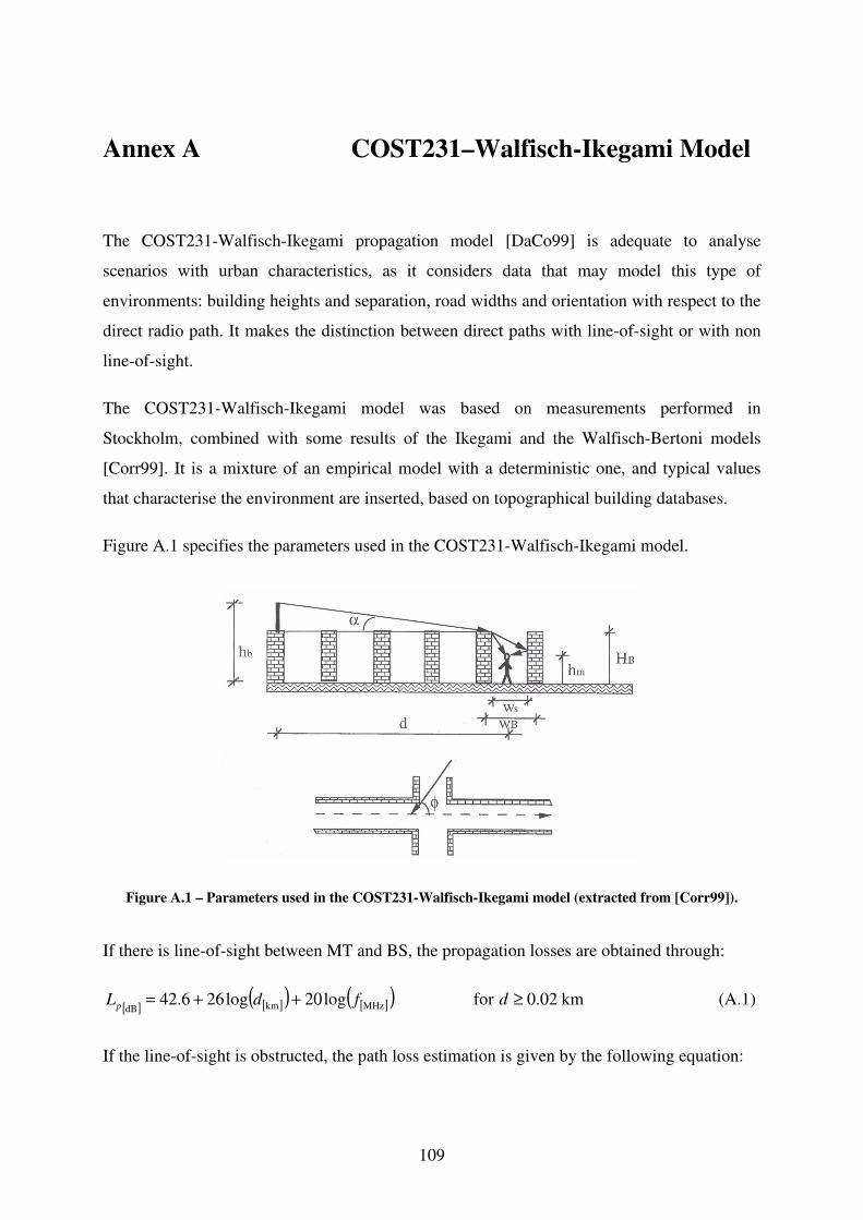
109
Annex A COST231–Walfisch-Ikegami Model
The COST231-Walfisch-Ikegami propagation model [DaCo99] is adequate to analyse
scenarios with urban characteristics, as it considers data that may model this type of
environments: building heights and separation, road widths and orientation with respect to the
direct radio path. It makes the distinction between direct paths with line-of-sight or with non
line-of-sight.
The COST231-Walfisch-Ikegami model was based on measurements performed in
Stockholm, combined with some results of the Ikegami and the Walfisch-Bertoni models
[Corr99]. It is a mixture of an empirical model with a deterministic one, and typical values
that characterise the environment are inserted, based on topographical building databases.
Figure A.1 specifies the parameters used in the COST231-Walfisch-Ikegami model.
Figure A.1 – Parameters used in the COST231-Walfisch-Ikegami model (extracted from [Corr99]).
If there is line-of-sight between MT and BS, the propagation losses are obtained through:
[ ] [ ]( ) [ ]( ) km02.0forlog20log266.42 MHzkmdB≥++= dfdLp (A.1)
If the line-of-sight is obstructed, the path loss estimation is given by the following equation:

A. COST231 – WI Propagation Model
110
[ ][ ] [ ] [ ]
[ ]
0 dB dB dB
dB0 dB for 0
rts msd
prts msd
L L LL
L L L
+ +��= � + ≤��
(A.2)
where each of these components reflect:
• L0 free space loss
• Lrts roof-top-to-street diffraction and scatter loss
• Lmsd multi-screen loss
The free space loss is given by:
[ ] [ ]( ) [ ]( )MHzkmdB0 log20log204.32 fdL ++= (A.3)
The roof-top-to-street diffraction and scatter loss is obtained through:
[ ] [ ]( ) [ ]( ) [ ] [ ]( ) [ ]dBmmMHzmdB log20log10log109.16 orimBsrts LhHfwL +−++−−= (A.4)
where:
[ ]
[ ]
[ ]( )[ ]( )
dB
10 0.354 for 0 35
2.5 0.075 35 for 35 55
4.0 0.114 55 for 55 90
rtsL
φ φ
φ φ
φ φ
� − + ≤ <��= + − ≤ <��� − − ≤ ≤�
� �
�
� �
�
� �
�
(A.5)
The multi-screen loss may be calculated via:
[ ] [ ] [ ]( ) [ ]( ) [ ]( )mMHzkmdBdB log9loglog Bfdabshmsd wfkdkkLL −+++= (A.6)
where:
[ ][ ] [ ]( )
���
≤
>−+−=
Bb
BbBbbsh Hh
HhHhL
0
1log18 mmdB (A.7)
[ ] [ ]( )[ ] [ ]( ) [ ]�
��
���
�
≤<×−×−
≤≥−×−>
=
BbBb
BbBb
Bb
a
HhddHh
HhdHh
Hh
k
andkm5.06.154
andkm5.08.054
54
kmmm
mm (A.8)
A. COST231 – WI Propagation Model
111
[ ] [ ]
[ ]��
��
�
≤−
×−
>=
BbB
Bb
Bb
d HhH
Hh
Hh
k
m
mm1518
18
(A.9)
[ ]
[ ]
MHz
MHz
for medium sized cities and suburban4 0.7 1
centres with moderate tree density925
5 1 for metropolitan centres925
f
f
k f
� � �− + × −� � �� �� � ��= � � �� × −� �� �� � ���
(A.10)
In case the data on the structure of the buildings and roads is unknown, it is recommended to
use the following values:
• Building separation (wB) ∈ [20, 50] m
• Widths of roads (ws) ws = 0.5 × wB
• Heights of buildings (HB) HB = 3 × {number of floors} + Hroof
• Roof height (Hroof) [ ]���
=flat,0pitched,3
mroofH
• Road orientation with respect to the direct radio path (φ) φ = 90°
The validity ranges of the COST231-Walfisch-Ikegami model correspond to:
• Frequency (f) ∈ [800, 2000] MHz
• BS height (hb) ∈ [4, 50] m
• MT height (hm) ∈ [1, 3] m
• Distance (d) ∈ [0.02, 5] km

112

113
Annex B Statistical distributions
Random variables arise in many applications, the sequence of incidents being commonly non-
correlated events. The occurrences of these variables reflect often models of fundamental
mechanisms that lie behind a random behaviour. Two statistical distributions, namely Poisson
and Exponential, which were referred along this thesis, are presented hereafter.
For the message arrival process the most common description is given in terms of Poisson
statistics. Poisson statistics are based on a discrete distribution of events, as presented in
Figure B.1.
Arrivals Time between Arrivalsarrivals
t 0 t 1 t 2 t 3 t 4 t 5
Time t
τ
Figure B.1 – Discrete distribution of events (extracted from [Keis89]).
The messages arrive at the system at times t0, t1, t2, … where t0 < t1 < t2 … < tn.
Taking into consideration an infinite source number (i.e., there is a large number of
independent users), the probability Pn(t) of exactly n users arriving during a time interval of
length t, according to Poisson’s distribution, is given by [Keis89]:
( ) ( )!
n t
n
t eP t
n
λλ −
= (B.1)
where:
• n = 0, 1, 2, …
• λ mean call arrival rate
• t time interval in which the call arrives
B. Statistical distributions
114
The Poisson distribution is frequently used to model call arrival times. The average or
expected number of arrivals in the time interval T is thus:
[ ] ( )0
nn
E N nP t Tλ∞
=
= = ⋅� (B.2)
The expected number of arrivals in the time interval (0, T) is equal to λ⋅T.
Considering that users enter the queuing system at times t0, t1, t2, …, tn, the random variables
τn = tn - tn-1 are called the inter-arrival times, that can be assumed to form a sequence of
independent and identically distributed random variables. Letting τ represent an arbitrary
inter-arrival time having a probability density function f(t), it can be said that Poisson arrivals
generate an exponential probability density:
( ) tf t e λλ − ⋅= (B.3)
It is further assumed, when considering the traffic model analysed along this thesis, that the
service time distribution, S(t), is given by (B.4):
( ) tS t e µµ − ⋅= (B.4)
where:
• µ service rate
The service time varies in a statistical way because the messages themselves vary randomly in
length.

115
Annex C Scenario A, Program results
Scenario A takes into account the number of users referred in Table 5.1: a considerable
amount of voice calls and rather few data. The program is first run for a cell with 150 m
radius; average speeds of 15 km/h and 60 km/h and buffer sizes of 20 and 10 MB are applied
in particular situations. The program is run a second time for a cell with 250 m radius.
The numbers of codes obtained are presented in Figure C.1:
(a) Equitable distribution of channels. (b) Proportional distribution of channels.
Figure C.1 – Number of codes for Scenario A with a 150 and 250 m cell radius.
The performance results, as a function of users’ speed, are presented in Figure C.2 to
Figure C.5, and as a function of the buffer size, correspond to Figure C.6 to Figure C.9.
Figure C.10 to Figure C.13 show the pij and pij’ matrices for a cell with 150 m radius, whereas
the results for a 250 m cell are presented in Figure C.14 to Figure C.17.

C. Scenario A, Program results
116
(a) Equitable distribution of channels.
(b) Proportional distribution of channels.
Figure C.2 – System performance versus users’ speed (150 m cell radius; 20 MB buffer size).
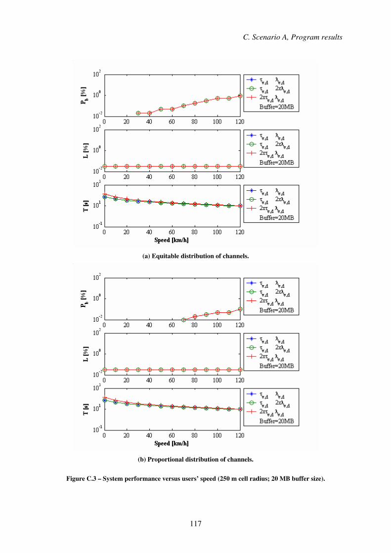
C. Scenario A, Program results
117
(a) Equitable distribution of channels.
(b) Proportional distribution of channels.
Figure C.3 – System performance versus users’ speed (250 m cell radius; 20 MB buffer size).

C. Scenario A, Program results
118
(a) Equitable distribution of channels.
(b) Proportional distribution of channels.
Figure C.4 – System performance versus users’ speed (150 m cell radius; 10 MB buffer size).

C. Scenario A, Program results
119
(a) Equitable distribution of channels.
(b) Proportional distribution of channels.
Figure C.5 – System performance versus users’ speed (250 m cell radius; 10 MB buffer size).

C. Scenario A, Program results
120
(a) Equitable distribution of channels.
(b) Proportional distribution of channels.
Figure C.6 – System performance versus buffer size (150 m cell radius; 15 km/h average speed).
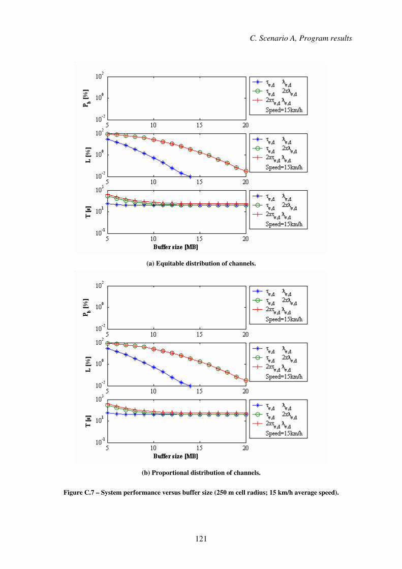
C. Scenario A, Program results
121
(a) Equitable distribution of channels.
(b) Proportional distribution of channels.
Figure C.7 – System performance versus buffer size (250 m cell radius; 15 km/h average speed).

C. Scenario A, Program results
122
(a) Equitable distribution of channels.
(b) Proportional distribution of channels.
Figure C.8 – System performance versus buffer size (150 m cell radius; 60 km/h average speed).
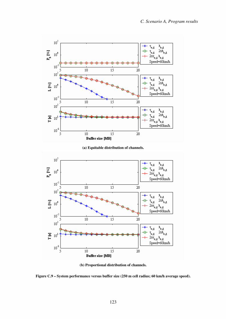
C. Scenario A, Program results
123
(a) Equitable distribution of channels.
(b) Proportional distribution of channels.
Figure C.9 – System performance versus buffer size (250 m cell radius; 60 km/h average speed).

C. Scenario A, Program results
124
(a) pij for an equitable distribution of resources.
(b) pij’ for an equitable distribution of resources.
Figure C.10 – Steady-states [(ττττv, ττττd), (λλλλv, λλλλd)], equitable distribution of resources and 150 m cell radius.
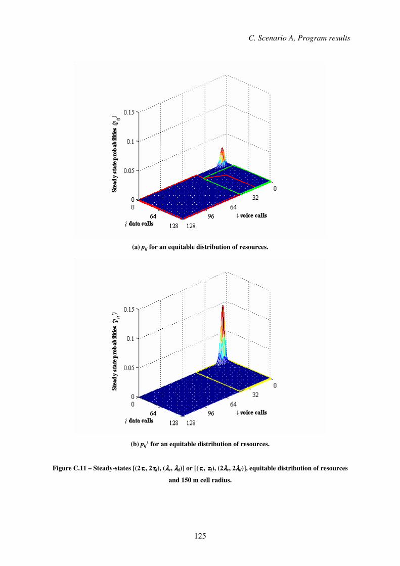
C. Scenario A, Program results
125
(a) pij for an equitable distribution of resources.
(b) pij’ for an equitable distribution of resources.
Figure C.11 – Steady-states [(2ττττv, 2ττττd), (λλλλv, λλλλd)] or [(ττττv, ττττd), (2λλλλv, 2λλλλd)], equitable distribution of resources
and 150 m cell radius.

C. Scenario A, Program results
126
(a) pij for a proportional distribution of resources.
(b) pij’ for a proportional distribution of resources.
Figure C.12 – Steady-states [(ττττv, ττττd), (λλλλv, λλλλd)], proportional distribution of resources and 150 m cell radius.

C. Scenario A, Program results
127
(a) pij for a proportional distribution of resources.
(b) pij’ for a proportional distribution of resources.
Figure C.13 – Steady-states [(2ττττv, 2ττττd), (λλλλv, λλλλd)] or [(ττττv, ττττd), (2λλλλv, 2λλλλd)], proportional distribution of
resources and 150 m cell radius.

C. Scenario A, Program results
128
(a) pij for an equitable distribution of resources.
(b) pij’ for an equitable distribution of resources.
Figure C.14 – Steady-states [(ττττv, ττττd), (λλλλv, λλλλd)], equitable distribution of resources and 250 m cell radius.

C. Scenario A, Program results
129
(a) pij for an equitable distribution of resources.
(b) pij’ for an equitable distribution of resources.
Figure C.15 – Steady-states [(2ττττv, 2ττττd), (λλλλv, λλλλd)] or [(ττττv, ττττd), (2λλλλv, 2λλλλd)], equitable distribution of resources
and 250 m cell radius.

C. Scenario A, Program results
130
(a) pij for a proportional distribution of resources.
(b) pij’ for a proportional distribution of resources.
Figure C.16 – Steady-states [(ττττv, ττττd), (λλλλv, λλλλd)], proportional distribution of resources and 250 m cell radius.

C. Scenario A, Program results
131
(a) pij for a proportional distribution of resources.
(b) pij’ for a proportional distribution of resources.
Figure C.17 – Steady-states [(2ττττv, 2ττττd), (λλλλv, λλλλd)] or [(ττττv, ττττd), (2λλλλv, 2λλλλd)], proportional distribution of
resources and 250 m cell radius.

132

133
Annex D Scenario B, Program results
Scenario B takes into account the number of users referred in Table 5.1, i.e., voice users will
load considerably less the system than data users. The program is first run for a cell with
150 m radius; average speeds of 15 km/h and 60 km/h and buffer sizes of 20 and 10 MB are
applied in particular situations. The program is run a second time for a cell with 250 m radius.
The numbers of channels obtained are presented in Figure D.1:
(a) Equitable distribution of channels. (b) Proportional distribution of channels.
Figure D.1 – Number of channels for Scenario B.
The performance results, as a function of users’ speed, are presented in Figure D.2 to
Figure D.5, and as a function of the buffer size, correspond to Figure D.6 to Figure D.9.
Figure D.10 to Figure D.13 show the pij and pij’ matrices for a cell with 150 m radius, whereas
the results for a 250 m cell are presented in Figure D.14 to Figure D.17.

D. Scenario B, Program results
134
(a) Equitable distribution of channels.
(b) Proportional distribution of channels.
Figure D.2 – System performance versus users’ speed (150 m cell radius; 20 MB buffer size).

D. Scenario B, Program results
135
(a) Equitable distribution of channels.
(b) Proportional distribution of channels.
Figure D.3 – System performance versus users’ speed (250 m cell radius; 20 MB buffer size).
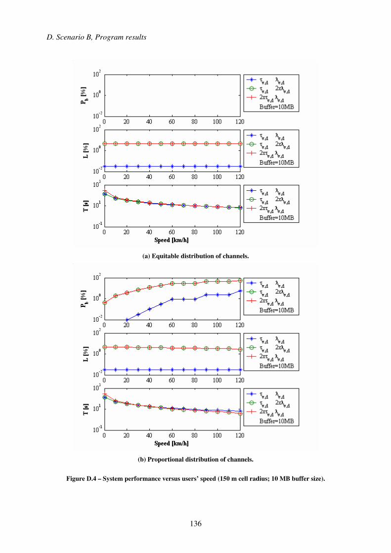
D. Scenario B, Program results
136
(a) Equitable distribution of channels.
(b) Proportional distribution of channels.
Figure D.4 – System performance versus users’ speed (150 m cell radius; 10 MB buffer size).

D. Scenario B, Program results
137
(a) Equitable distribution of channels.
(b) Proportional distribution of channels.
Figure D.5 – System performance versus users’ speed (250 m cell radius; 10 MB buffer size).

D. Scenario B, Program results
138
(a) Equitable distribution of channels.
(b) Proportional distribution of channels.
Figure D.6 – System performance versus buffer size (150 m cell radius; 15 km/h average speed).
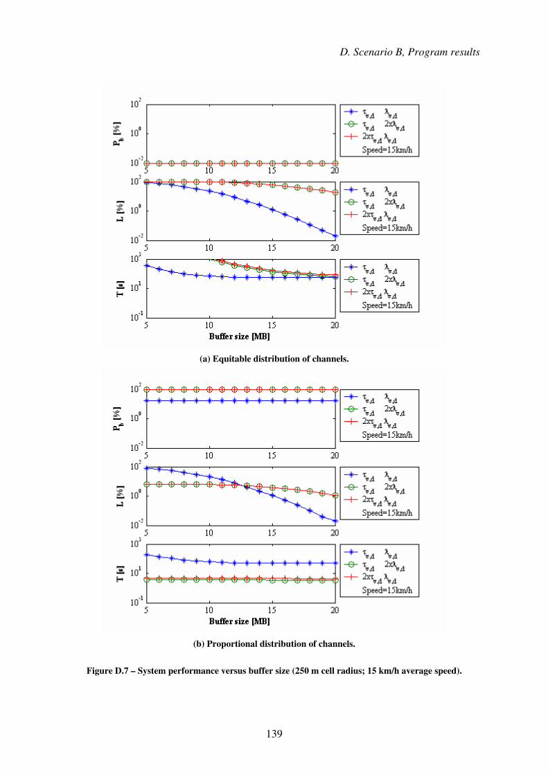
D. Scenario B, Program results
139
(a) Equitable distribution of channels.
(b) Proportional distribution of channels.
Figure D.7 – System performance versus buffer size (250 m cell radius; 15 km/h average speed).
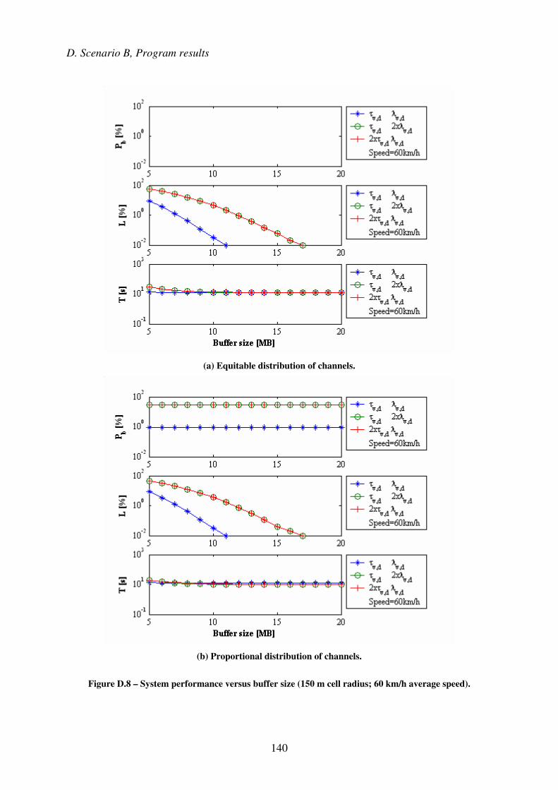
D. Scenario B, Program results
140
(a) Equitable distribution of channels.
(b) Proportional distribution of channels.
Figure D.8 – System performance versus buffer size (150 m cell radius; 60 km/h average speed).
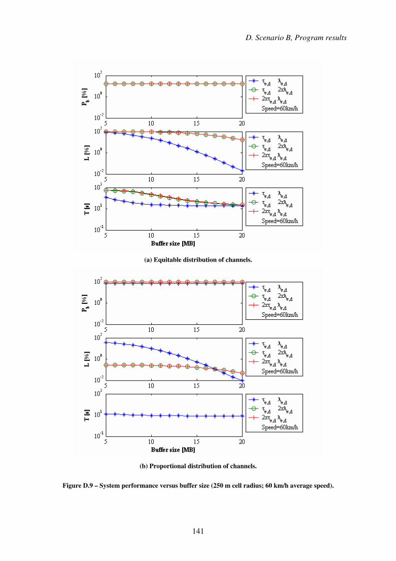
D. Scenario B, Program results
141
(a) Equitable distribution of channels.
(b) Proportional distribution of channels.
Figure D.9 – System performance versus buffer size (250 m cell radius; 60 km/h average speed).
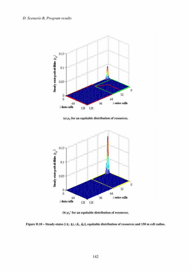
D. Scenario B, Program results
142
(a) pij for an equitable distribution of resources.
(b) pij’ for an equitable distribution of resources.
Figure D.10 – Steady-states [(ττττv, ττττd), (λλλλv, λλλλd)], equitable distribution of resources and 150 m cell radius.
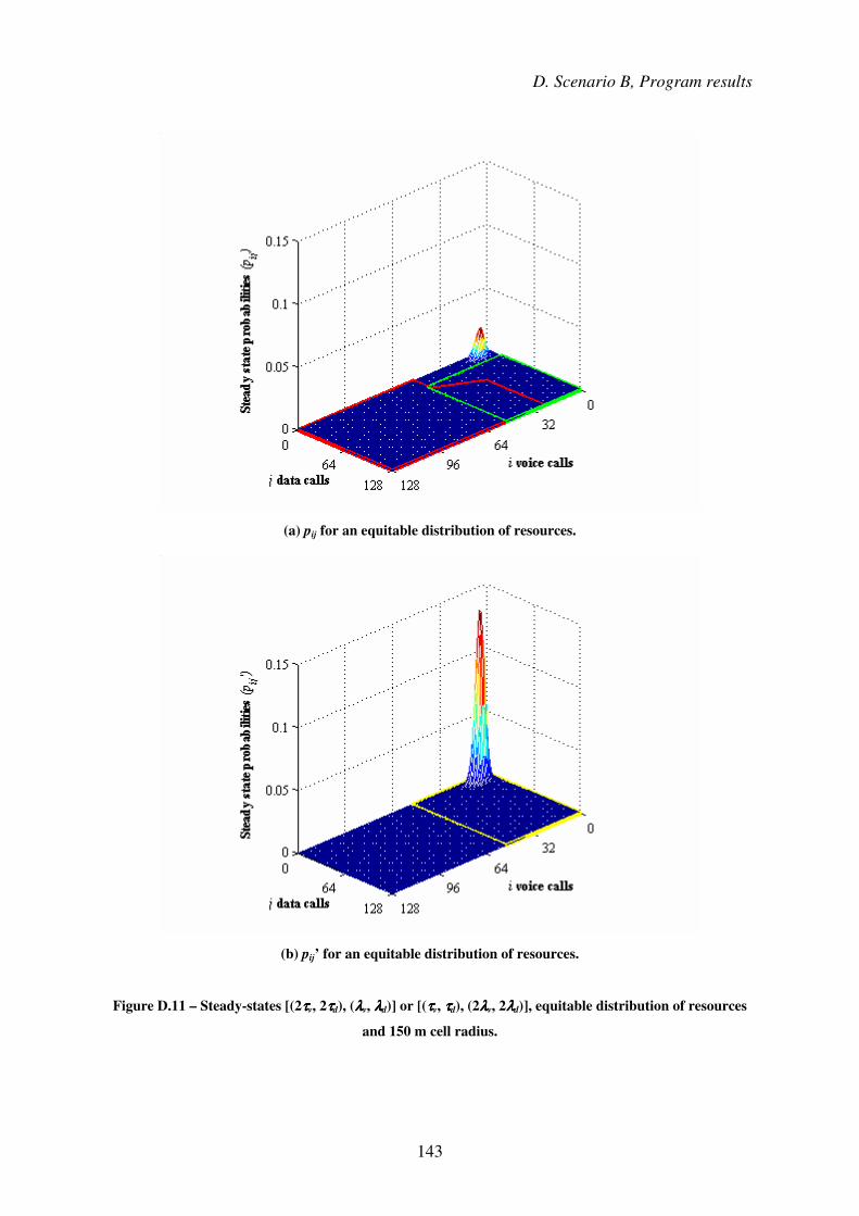
D. Scenario B, Program results
143
(a) pij for an equitable distribution of resources.
(b) pij’ for an equitable distribution of resources.
Figure D.11 – Steady-states [(2ττττv, 2ττττd), (λλλλv, λλλλd)] or [(ττττv, ττττd), (2λλλλv, 2λλλλd)], equitable distribution of resources
and 150 m cell radius.
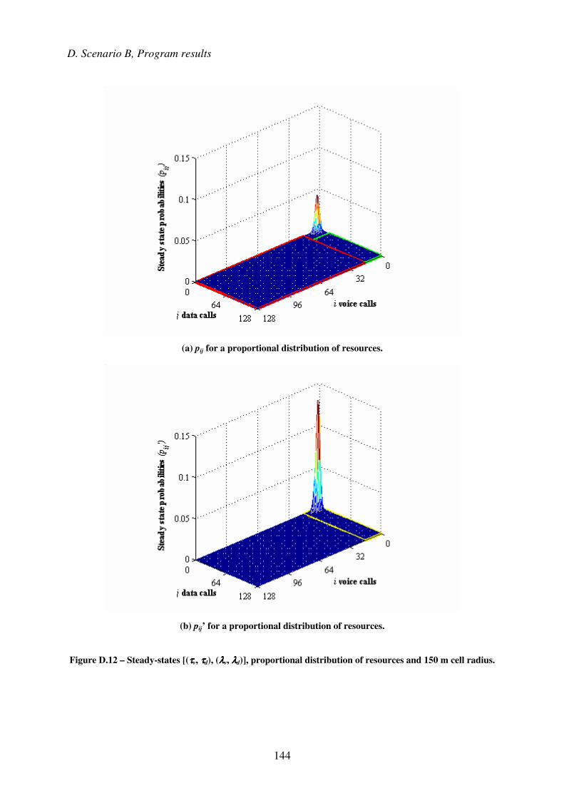
D. Scenario B, Program results
144
(a) pij for a proportional distribution of resources.
(b) pij’ for a proportional distribution of resources.
Figure D.12 – Steady-states [(ττττv, ττττd), (λλλλv, λλλλd)], proportional distribution of resources and 150 m cell radius.

D. Scenario B, Program results
145
(a) pij for a proportional distribution of resources.
(b) pij’ for a proportional distribution of resources.
Figure D.13 – Steady-states [(2ττττv, 2ττττd), (λλλλv, λλλλd)] or [(ττττv, ττττd), (2λλλλv, 2λλλλd)], proportional distribution of
resources and 150 m cell radius.
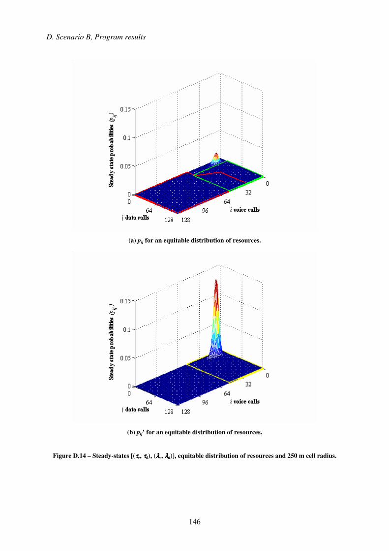
D. Scenario B, Program results
146
(a) pij for an equitable distribution of resources.
(b) pij’ for an equitable distribution of resources.
Figure D.14 – Steady-states [(ττττv, ττττd), (λλλλv, λλλλd)], equitable distribution of resources and 250 m cell radius.

D. Scenario B, Program results
147
(a) pij for an equitable distribution of resources.
(b) pij’ for an equitable distribution of resources.
Figure D.15 – Steady-states [(2ττττv, 2ττττd), (λλλλv, λλλλd)] or [(ττττv, ττττd), (2λλλλv, 2λλλλd)], equitable distribution of resources
and 250 m cell radius.

D. Scenario B, Program results
148
(a) pij for a proportional distribution of resources.
(b) pij’ for a proportional distribution of resources.
Figure D.16 – Steady-states [(ττττv, ττττd), (λλλλv, λλλλd)], proportional distribution of resources and 250 m cell radius.

D. Scenario B, Program results
149
(a) pij for a proportional distribution of resources.
(b) pij’ for a proportional distribution of resources.
Figure D.17 – Steady-states [(2ττττv, 2ττττd), (λλλλv, λλλλd)] or [(ττττv, ττττd), (2λλλλv, 2λλλλd)], proportional distribution of
resources and 250 m cell radius.

150

151
References
[3GPP00a] 3GPP, Spreading and Modulation (TDD), Technical Specification Group
– Radio Access Network, Report No. 25.223 Ver. 3.2.0, Mar. 2000
(http://www.3gppg.org).
[3GPP01a] 3GPP, UTRAN Overall Description, Technical Specification Group –
Radio Access Network, Report No. 25.401 Ver. 4.0.0, Mar. 2001
(http://www.3gppg.org).
[3GPP01b] 3GPP, Spreading and Modulation (FDD), Technical Specification Group
– Radio Access Network, Report No. 25.213 Ver. 3.5.0, Mar. 2001
(http://www.3gppg.org).
[3GPP01c] 3GPP, UE Radio Transmission and Reception (FDD), Technical
Specification Group – Radio Access Network, Report No. 25.101
Ver. 5.0.0, Sep. 2001 (http://www.3gppg.org).
[3GPP02a] 3GPP, Quality of Service (QoS) concept and architecture, Technical
Specification Group – Services and System Aspects, Report No. 23.107
Ver. 5.6.0, Sep. 2002 (http://www.3gppg.org).
[3GPP02b] 3GPP, Physical channels and mapping of transport channels onto
physical channels (FDD), Technical Specification Group – Radio Access
Network, Report No. 25.211 Ver. 3.12.0, Sep. 2002
(http://www.3gppg.org).
[3GPP02c] 3GPP, Physical channels and mapping of transport channels onto
physical channels (TDD), Technical Specification Group – Radio Access
Network, Report No. 25.221 Ver. 3.11.0, Sep. 2002
(http://www.3gppg.org).
References
152
[3GPP03] 3GPP, Vocabulary for 3GPP Specifications, Technical Specification
Group – Services and System Aspects, Report No. 21.905 Ver. 5.8.0,
Sep. 2003 (http://www.3gppg.org).
[3GPP99a] 3GPP, Physical Layer – General Description, Technical Specification
Group – Radio Access Network, Report No. 25.201 Ver. 3.0.1, Dec. 1999
(http://www.3gppg.org).
[CaVa02] Carvalho,P. and Vasconcelos,A., Traffic Models for Base Stations in
UMTS (in Portuguese), Graduation Report, Instituto Superior Técnico,
Lisbon, Portugal, Sep. 2002.
[CEPT00] CEPT, Detailed Spectrum Investigation Phase III, European
Radiocommunications Committee, Final Report on DSI Phase III,
Apr. 2000 (http://www.ero.dk).
[CEPT02] CEPT, European Common Allocation Table, European
Radiocommunications Committee, ERC Report 25, Jan. 2002
(http://www.ero.dk).
[Corr03] Correia,L.M., Mobile and Personal Communication Systems (in
Portuguese), Course Notes, Instituto Superior Técnico, Lisbon, Portugal,
May 2003 (http://fenix3.ist.utl.pt/publico)
[Corr99] Correia L.M., Mobile Communications – Parts I and II (in Portuguese),
Course Notes, Instituto Superior Técnico, Lisbon, Portugal, Mar. 1999.
[DaCo99] Damosso,E. and Correia,L.M., Digital Mobile Radio Towards Future
Generation Systems – COST 231 Final Report, COST Office, Brussels,
Belgium, 1999.
[Dias03] Dias,C., Traffic Analysis at the Radio Interface in UMTS FDD, Master
Thesis, Instituto Superior Técnico, Lisbon, Portugal, Dec. 2003.

References
153
[ETSI01] ETSI, General Packet Radio Service (GPRS); Mobile Station – Serving
GPRS Support Node (MS-SGSN) Logical Link Control (LLC) Layer
Specification, Report No. 101 351 Ver. 8.7.0, Sophia-Antipolis, France,
Dec. 2001 (http://www.etsi.org).
[ETSI98] ETSI, Selection procedures for the choice of radio transmission
technologies of the UMTS (UMTS 30.03 version 3.2.0), Report TR 101
112 Ver. 3.2.0, Sophia-Antipolis, France, Apr. 1998 (http://www.etsi.org).
[FCSC02] Ferreira,L., Correia,L.M., Serrador,A., Carvalho,G., Fledderus,E. and
Perera,R., UMTS Deployment and Mobility Scenarios, IST-
MOMENTUM Project, Deliverable D1.3, IST-TUL, Lisbon, Portugal,
Oct. 2002 (http://momentum.zib.de).
[FCXV03] Ferreira,L., Correia,L.M., Xavier,D., Vasconcelos,A. and Fledderus,E.,
Final Report on Traffic Estimation and Services Characterisation, IST-
MOMENTUM Project, Deliverable D1.4, IST-TUL, Lisbon, Portugal,
May 2003, (http://momentum.zib.de).
[FMSC01] Ferreira,L., Marques,G., Serrador,A. and Correia,L.M., Classification of
Mobile Multimedia Services, IST-MOMENTUM Project, Deliverable
D1.1, IST-TUL, Lisbon, Portugal, Dec. 2001 (http://momentum.zib.de).
[HaLH00] Haung,Y.-R., Lin,Y.-B. and Ho,J.-M., Performance Analysis for
Voice/Data Integration on a Finite-Buffer Mobile System, IEEE
Transactions on Vehicular Technology, Vol. 49, No. 2, Mar. 2000,
pp. 367-378.
[HaLi97] Hanselman,D. and Littlefield,B., The Student Edition of Matlab, Prentice
Hall, Upper Saddle River, NJ, USA, 1997 (http://www.mathworks.com/).
[HoTo01] Holma,H. and Toskala,A., WCDMA for UMTS, John Wiley & Sons,
Chichester, UK, 2001.
References
154
[Jabb96] Jabbari,B., “Teletraffic Aspects of Evolving and Next-Generation
Wireless Communication Networks”, IEEE Personal Communications,
Vol. 3, No. 6, Dec. 1996, pp. 4-9.
[Keis89] Keiser,G.E., Local Area Networks, McGraw-Hill, Singapore, 1989.
[KeRi88] Kernighan,B.W. and Ritchie,D.M., The C Programming Language,
Prentice Hall, Englewood Cliffs, NJ, USA, 1988.
[Leon94] Leon-Garcia,A., Probability and Random Processes for Electrical
Engineering, Addison-Wesley, Massachusetts, USA, 1994.
[Meye84] Meyer,P.L., Introductory Probability and Statistical Applications (in
Portuguese), Livros Técnicos e Científicos Editora, Rio de Janeiro, Brazil,
1984.
[MOME01] MOMENTUM, Models and Simulations for Network Planning and
Control of UMTS, IST-MOMENTUM Project
(http://www.zib.de/projects/telecommunication/MOMENTUM/).
[MSDN03] Microsoft Developer Network Online (http://msdn.microsoft.com).
[Rapp96] Rappaport,T.S., Wireless Communications, Prentice Hall, NJ, USA, 1996.
[RFHL03] Rakoczi,B., Fledderus,E., Heideck,B., Lourenço,P. and Kürner,T.,
Reference Scenarios, IST-MOMENTUM Project, Deliverable D5.2, KPN,
The Hague, The Netherlands, Nov. 2003.
[SeCo03] Serrador,A. and Correia,L.M., Protocol Buffering Effects on Traffic, IST-
FLOWS Project, Internal Report No. WP6_IST-TUL_TN_INT_065_01,
IST-TUL, IST, Lisbon, Portugal, July 2003.
[Serr02] Serrador,A., Optimisation of Cell Radius in UMTS-FDD Networks,
Master Thesis, Instituto Superior Técnico, Lisbon, Portugal, Dec. 2002.

References
155
[TWPL02] Türke,U., Winter,T., Perera,R., Lamers,E., Meijerink,E., Fledderus,E. and
Serrador,A., Comparison of different simulation approaches for cell
performance evaluation, IST-MOMENTUM Project, Deliverable D2.2,
Siemens, Berlin, Germany, Oct. 2002 (http://momentum.zib.de).
[UMTS01] UMTS Forum, The UMTS Third Generation Market – Phase II:
Structuring the Service Revenue Opportunities, Report No. 13, London,
UK, Apr. 2001 (http://www.umts-forum.org/).
[UMTS98] UMTS Forum, UMTS/IMT-2000, Report No. 6, London, UK, Dec.1998
(http://www.umts-forum.org/).
[Voda02] Vodafone-Telecel, IST-MOMENTUM Project, WP5 Reference Scenarios
CD, Lisbon, Portugal, Oct. 2002.
[Yaco93] Yacoub,M.D., Foundations of Mobile Radio Engineering, CRC Press,
Boca Raton, FL, USA, 1993.

156