AMS 212B Perturbation Methods - University of California...
18
- 1 - AMS 212B Perturbation Methods Lecture 04 Copyright by Hongyun Wang, UCSC Recap • Non-dimensionalization, identifying time scale, length scale identifying small parameter, • Asymptotic series of ƒ(x, ϵ) IVP of ODE oscillation of pendulum straightforward expansion is invalid for large t. period of oscillation A brief look at Laplace transform Consider function ƒ(t). Laplace transform of ƒ(t) is defined as L ft () ⎡ ⎣ ⎤ ⎦ s () Full notation ! " # $ ## ≡ e − st ft () dt 0 ∞ ∫ Other notations: Fs () , L ft () ⎡ ⎣ ⎤ ⎦ We start with the L-transform of e at . Example: Le at ⎡ ⎣ ⎤ ⎦ = e − s −a ( ) t dt 0 ∞ ∫ = 1 s − a L-transform of derivatives with respect to a parameter L d da ft , a ( ) ⎡ ⎣ ⎢ ⎤ ⎦ ⎥ = d da L ft , a ( ) ⎡ ⎣ ⎤ ⎦ Example: 1 = e at a=0
Transcript of AMS 212B Perturbation Methods - University of California...
- 1 -
AMS212BPerturbationMethodsLecture04
CopyrightbyHongyunWang,UCSC
Recap
• Non-dimensionalization,identifyingtimescale,lengthscaleidentifyingsmallparameter,
• Asymptoticseriesofƒ(x,ϵ)IVPofODEoscillationofpendulumstraightforwardexpansionisinvalidforlarget.periodofoscillation
AbrieflookatLaplacetransformConsiderfunctionƒ(t).
Laplacetransformofƒ(t)isdefinedas
L f t( )⎡⎣ ⎤⎦ s( )Fullnotation! "# $##
≡ e−st f t( )dt0
∞
∫
Othernotations: F s( ) , L f t( )⎡⎣ ⎤⎦
WestartwiththeL-transformofeat.
Example:
L eat⎡⎣ ⎤⎦ = e− s−a( )t dt
0
∞
∫ = 1s −a
L-transformofderivativeswithrespecttoaparameter
L dda
f t ,a( )⎡
⎣⎢
⎤
⎦⎥ =
ddaL f t ,a( )⎡⎣ ⎤⎦
Example:
1= eat
a=0
AMS212BPerturbationMethods
- 2 -
==>L 1⎡⎣ ⎤⎦ =
1s −a
⎛⎝⎜
⎞⎠⎟a=0
= 1s
Similarly,wecanderive
L tn⎡⎣ ⎤⎦ =
n!sn+1
Example:
L sinh at( )⎡⎣ ⎤⎦ = L
eat −e−at
2⎡
⎣⎢
⎤
⎦⎥ =
12
1s −a
− 1s +a
⎛⎝⎜
⎞⎠⎟= as2 −a2
L eiat⎡⎣ ⎤⎦ =
1s −ai
L sin at( )⎡⎣ ⎤⎦ = L
eiat −e− iat
2i⎡
⎣⎢
⎤
⎦⎥ =
12i
1s −ai
− 1s +ai
⎛⎝⎜
⎞⎠⎟= as2 +a2
L-transformofderivativeswithrespecttoindependentvariable
L ′f t( )⎡⎣ ⎤⎦ = sL f t( )⎡⎣ ⎤⎦− f 0( )
L ′′f t( )⎡⎣ ⎤⎦ = s2L f t( )⎡⎣ ⎤⎦− s f 0( )− ′f 0( )
FindinginverseL-transformusingderivativewithrespecttoaparameter
L−1 d
dag s ,a( )⎡
⎣⎢
⎤
⎦⎥ =
ddaL−1 g s ,a( )⎡⎣ ⎤⎦
Example:
L−1 s
s2 +a2( )2⎡
⎣
⎢⎢⎢
⎤
⎦
⎥⎥⎥= t2asin at( )
L−1 1
s2 +a2( )2⎡
⎣
⎢⎢⎢
⎤
⎦
⎥⎥⎥= ? Weusedifferentiationtofindthisone.
AMS212BPerturbationMethods
- 3 -
1s2 +a2( )2
= 1−2a( )
dda
1s2 +a2
⎛⎝⎜
⎞⎠⎟
L−1 1
s2 +a2( )2⎡
⎣
⎢⎢⎢
⎤
⎦
⎥⎥⎥= 1
−2a( )L−1 dda
1s2 +a2
⎛⎝⎜
⎞⎠⎟
⎡
⎣⎢
⎤
⎦⎥ =
1−2a( )
ddaL−1 1
s2 +a2⎡
⎣⎢
⎤
⎦⎥
= 1
−2a( )dda
1asin at( )⎛
⎝⎜⎞⎠⎟=sin at( )2a3 −
t cos at( )2a2
L−1 1
s2 +a2( )2⎡
⎣
⎢⎢⎢
⎤
⎦
⎥⎥⎥=sin at( )2a3 −
t cos at( )2a2
BoundaryValueProblem(BVP)ofODERegularperturbation
Example:
′′y − ε ′y −9y =0y 0( ) =0 , y 1( ) =1
⎧⎨⎪
⎩⎪
Weseekanexpansionoftheform
y x ,ε( ) = a0 x( )+ εa1 x( )+!
Boundarycondition:
y(0)=0 ==> a0 0( )+ εa1 0( )+!=0
==> a0 0( ) =0 , a1 0( ) =0 y(1)=1 ==> a0 1( )+ εa1 1( )+!=1
==> a0 1( ) =1 , a1 1( ) =0 Substitutingtheexpansionintotheequation,wehave
′′a0 + ε ′′a1⎡⎣ ⎤⎦− ε ′a0⎡⎣ ⎤⎦−9 a0 + εa1⎡⎣ ⎤⎦ =0
==> ′′a0 −9a0⎡⎣ ⎤⎦+ ε ′′a1 −9a1 − ′a0⎡⎣ ⎤⎦+!=0
AMS212BPerturbationMethods
- 4 -
ε0:
′′a0 −9a0 =0a0 0( ) =0 , a0 1( ) =1
⎧⎨⎪
⎩⎪
WeuseLaplacetransformtosolveit.
LetA s( ) = L a0 x( )⎡⎣ ⎤⎦
Recall
L ′f x( )⎡⎣ ⎤⎦ = sL f x( )⎡⎣ ⎤⎦− f 0( )
L ′′f x( )⎡⎣ ⎤⎦ = s2L f x( )⎡⎣ ⎤⎦− s f 0( )− ′f 0( )
TakingLaplacetransformofbothsides,wehave
s2A s( )− sa0 0( )− ′a0 0( )−9A s( ) =0
Letα=a0’(0),unknownforthetimebeing.Wehave
s2 −32( )A s( ) =α
==>A s( ) =α 1
s −3( ) s +3( )
==>A s( ) = α
61s −3−
1s +3
⎛⎝⎜
⎞⎠⎟
==>a0 x( ) = L−1 A s( )⎡⎣ ⎤⎦ =
α6 e3x −e−3x( )
Enforcingtheboundaryconditiona0(1)=1todetermineα
==>a0 x( ) = L−1 A s( )⎡⎣ ⎤⎦ =
α6 e3x −e−3x( )
ε1:
′′a1 −9a1 = ′a0 =3
e3 −e−3e3x +e−3x( )
a1 0( ) =0 , a1 1( ) =0
⎧
⎨⎪⎪
⎩⎪⎪
(Skipthederivationinlecture)WeuseLaplacetransformtosolveit.
LetA s( ) = L a1 x( )⎡⎣ ⎤⎦
TakingLaplacetransformofbothsides,wehave
AMS212BPerturbationMethods
- 5 -
s2A s( )− sa1 0( )− ′a1 0( )−9A s( ) = q 1
s −3+1s +3
⎛⎝⎜
⎞⎠⎟, q= 3
e3 −e−3
Letα=a1’(0).Wehave
==>s2 −32( )A s( ) =α+q 1
s −3+1s +3
⎛⎝⎜
⎞⎠⎟
==>A s( ) = 16
1s −3−
1s +3
⎛⎝⎜
⎞⎠⎟
α+q 1s −3+
1s +3
⎛⎝⎜
⎞⎠⎟
⎡
⎣⎢
⎤
⎦⎥
==>
A s( ) = α
61s −3−
1s +3
⎛⎝⎜
⎞⎠⎟+ q6
1s −3( )2
− 1s +3( )2
⎛
⎝⎜⎜
⎞
⎠⎟⎟
==>
a1 x( ) = L−1 A s( )⎡⎣ ⎤⎦ =
α6 e3x −e−3x( )+ q6L
−1 1s −3( )2
− 1s +3( )2
⎡
⎣
⎢⎢⎢
⎤
⎦
⎥⎥⎥
Recall
L eat⎡⎣ ⎤⎦ =
1s −a
Differentiatingwithrespecttoa
==>
L t eat⎡⎣ ⎤⎦ =
1s −a( )2
L−1 1
s −a( )2⎡
⎣
⎢⎢⎢
⎤
⎦
⎥⎥⎥= t eat
Usingthisresulttocalculatea1(x),weobtain
a1 x( ) = α
6 e3x −e−3x( )+ q6 x e3x −e−3x( )
Enforcingtheboundaryconditiona1(1)=0todetermineα
==> α=−q
==>a1 x( ) = q6 x −1( ) e3x −e−3x( ) Recall
q= 3
e3 −e−3
==>a1 x( ) = 1
2 e3 −e−3( ) x −1( ) e3x −e−3x( )
Thus,thesolutionofBVPhastheexpansion
AMS212BPerturbationMethods
- 6 -
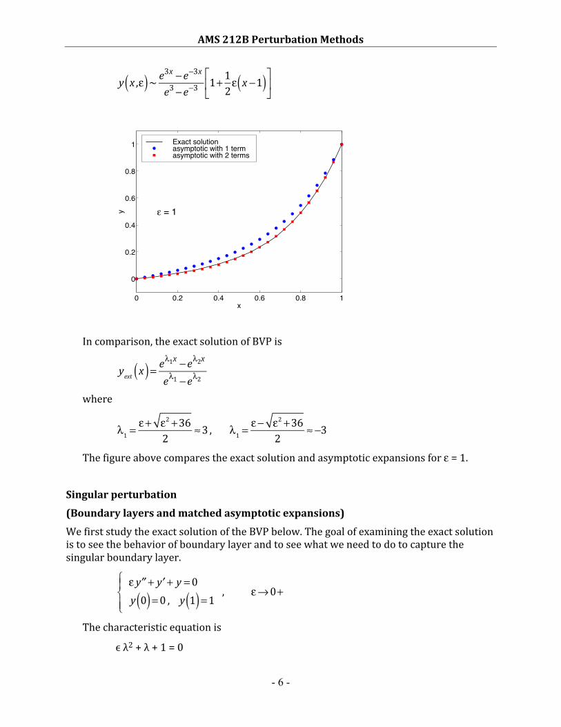
y x ,ε( )~ e
3x −e−3x
e3 −e−31+ 12ε x −1( )⎡
⎣⎢
⎤
⎦⎥
Incomparison,theexactsolutionofBVPis
yext x( ) = e
λ1x −eλ2x
eλ1 −eλ2
where
λ1 =
ε+ ε2 +362 ≈3 , λ1 =
ε− ε2 +362 ≈ −3
Thefigureabovecomparestheexactsolutionandasymptoticexpansionsforε=1.
Singularperturbation
(Boundarylayersandmatchedasymptoticexpansions)
WefirststudytheexactsolutionoftheBVPbelow.Thegoalofexaminingtheexactsolutionistoseethebehaviorofboundarylayerandtoseewhatweneedtodotocapturethesingularboundarylayer.
ε ′′y + ′y + y =0y 0( ) =0 , y 1( ) =1
⎧⎨⎪
⎩⎪, ε→0+
Thecharacteristicequationis
ϵλ2+λ+1=0
0 0.2 0.4 0.6 0.8 1
0
0.2
0.4
0.6
0.8
1
x
y ε = 1
Exact solutionasymptotic with 1 termasymptotic with 2 terms
AMS212BPerturbationMethods
- 7 -
Ithastwodistinctroots:
λ1 =
−1+ 1−4 ε2ε , λ2 =
−1− 1−4 ε2ε
Ageneralsolutionis
yext x( ) = c1eλ1x + c2eλ2x Enforcingtheboundaryconditionyields
yext x( ) = 1
eλ1 −eλ2eλ1x −eλ2x( )
Nowwelookatthebehaviorsofvarioustermsintheexactsolutionasε→0+.
Asε→0+,wehave
λ1 =−1+ 1−4 ε
2ε =−1+ 1− 12 ⋅4ε+O ε2( )⎛
⎝⎜⎞⎠⎟
2ε= −1+O ε( )→−1
λ2 =−1− 1−4 ε
2ε =−1− 1− 12 ⋅4ε+O ε2( )⎛
⎝⎜⎞⎠⎟
2ε
= −1ε+O 1( )→−∞
eλ1 = e−1+O ε( ) → e−1
eλ1x = e−1+O ε( )⎛
⎝⎜⎞⎠⎟x → e−x
eλ2x = e−1εx+O 1( )x ≈
0 , x >>O ε( )e−1ε x , x =O ε( )
⎧
⎨⎪
⎩⎪
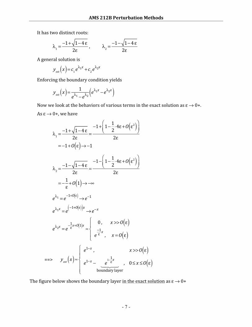
==>
yext x( )≈e1−x , x >>O ε( )e1−x − e
1−1εx
boundarylayer!"# $# , 0≤ x ≤O ε( )
⎧
⎨⎪⎪
⎩⎪⎪
Thefigurebelowshowstheboundarylayerintheexactsolutionasε→0+
AMS212BPerturbationMethods
- 8 -
Theboundarylayersuggeststhatweneedtwoasymptoticexpansions:
• Outerexpansion:outsidetheboundarylayer: x >>O ε( )
• Innerexpansion:insidetheboundarylayer: x =O ε( )
Belowwefirstusetheexactsolutiontoillustratetheouterexpansionandinnerexpansion.Later,wewillderivetheouterexpansionandinnerexpansiondirectlyfromdifferentialequationwithoutusingtheexactsolution.Outerexpansion:
Atafixedx>0(outsidetheboundarylayer),
limε→0+ yext x( ) = e1−x (Hereyext(x)istheexactsolution)
==> yout( ) x( ) = e1−x +!
Observation:
y(out)(x)satisfiesonlytheboundaryconditionatx=1
(attheendawayfromtheboundarylayer)Theboundaryconditionsare y(0)=0andy(1)=1.
y(out)(x)satisfiesonlyy out( ) x( )
x=1= e1−x
x=1=1 .
Atx=0,y out( ) x( )
x=0= e1−x
x=0= e ≠0 .
Innerexpansion:
0 0.2 0.4 0.6 0.8 1
0
0.5
1
1.5
2
2.5
x
y
ε = 0.05ε = 0.01
AMS212BPerturbationMethods
- 9 -
Fromtheexactsolution,weknowthewidthofboundarylayer=O(ε)asε→0+.
Inotherwords,asε→0+,thewidthofboundarylayer→0.
Togetridofthissingularityandtocapturetheboundarylayerasε→0+,weusescalingtointroduceaninnervariable
u= x
ε
Intermsofu,thewidthoftheboundarylayerisO(1).
Notation(Becareful!Thisnotationmaybeabitconfusing):
yext u( )≡ yext x( ) x=εu
Atafixedu(insidetheboundarylayer)
limε→0+ yext u( ) = limε→0+ e e
−εu −e−u( ) = e 1−e−u( ) ==> y
inn( ) u( ) = e 1−e−u( )+!
Observation:
y(inn)(u)satisfiesonlytheboundaryconditionatx=0
(attheboundarylayer)Theboundaryconditionsare y(0)=0andy(1)=1.
y(inn)(u)satisfiesonlyy inn( ) x
ε⎛⎝⎜
⎞⎠⎟x=0
= e 1−e−xε
⎛
⎝⎜⎞
⎠⎟x=0
=0 .
Atx=1,y inn( ) x
ε⎛⎝⎜
⎞⎠⎟x=1
= e 1−e−xε
⎛
⎝⎜⎞
⎠⎟x=1
≈ e ≠1 .
Letussummarizewhatwelearnedfromexaminingtheexactsolution.Summary:
Weneedtwoexpansions:
y(out)(x): outsidetheboundarylayerand
y(inn)(u): insidetheboundarylayerwithinnervariableu= x
ε.
Onlyoneboundaryconditionisimposedoneachofy(out)(x)andy(inn)(u).
y(out)(x)satisfiesonlytheboundaryconditionawayfromtheboundarylayer.
y(inn)(u)satisfiesonlytheboundaryconditionattheboundarylayer.
AMS212BPerturbationMethods
- 10 -
Question: In
ε ′′y + ′y + y =0y 0( ) =0 , y 1( ) =1
⎧⎨⎪
⎩⎪,whathappensifε→0-?
Weagainusetheexactsolutiontoanswerthisquestion.
yext x( ) = e
λ2x −eλ1x
eλ2 −eλ1
Asε→0-,wehave
λ1 =−1+ 1−4 ε
2ε =−1+ 1− 12 ⋅4ε+O ε2( )⎛
⎝⎜⎞⎠⎟
2ε= −1+O ε( )→−1
λ2 =−1− 1−4 ε
2ε =−1− 1− 12 ⋅4ε+O ε2( )⎛
⎝⎜⎞⎠⎟
2ε
= −1ε+O 1( )→ +∞
Were-writetheexactsolutionas
yext x( ) = e
λ2x −eλ1x
eλ2 −eλ1= e
λ2 x−1( ) −eλ1x−λ21−eλ1−λ2
eλ1−λ2 →0 eλ1x−λ2 →0
eλ2 x−1( ) = e
−1ε+O 1( )⎛
⎝⎜
⎞
⎠⎟ x−1( )
≈0 , 1− x( ) >>O ε( )
e−1ε x−1( ) , 1− x( ) =O ε( )
⎧
⎨⎪
⎩⎪
==>
yext x( )≈0 , 1− x( ) >>O ε( )e−1ε x−1( )
boundarylayer! "# $# , 1− x( ) =O ε( )
⎧
⎨⎪⎪
⎩⎪⎪
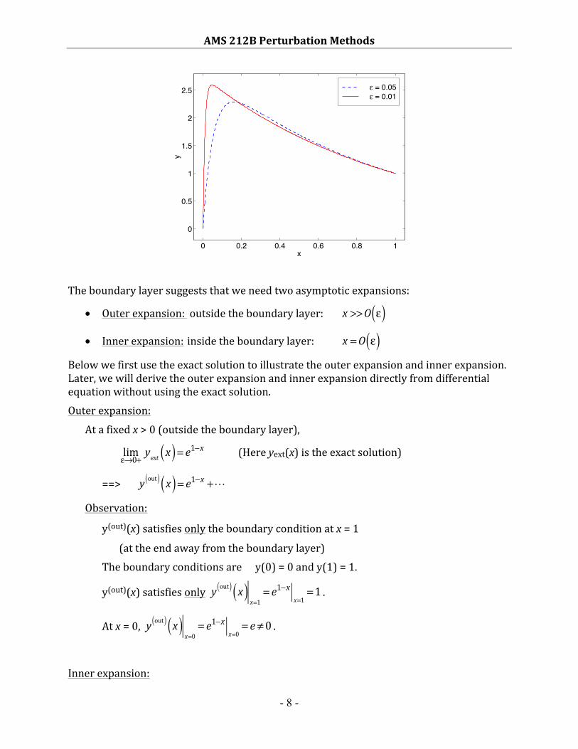
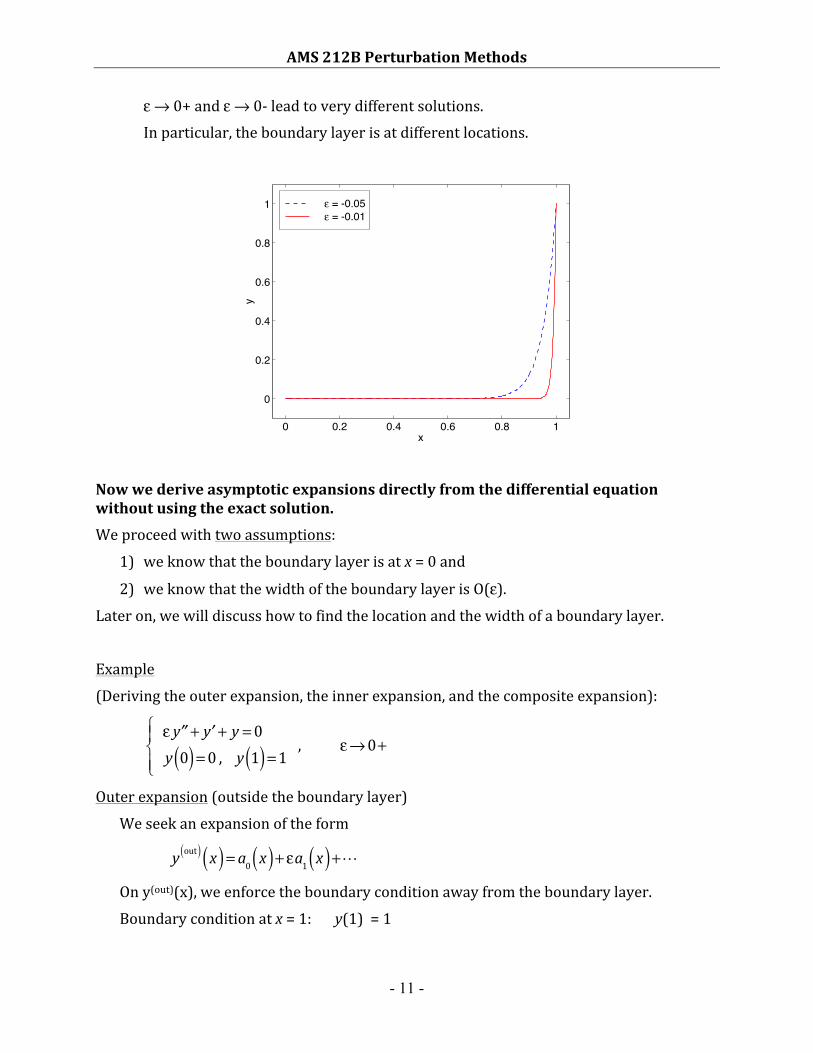
Thefigurebelowshowstheboundarylayerintheexactsolutionasε→0-.Remark:
AMS212BPerturbationMethods
- 11 -
ε→0+andε→0-leadtoverydifferentsolutions.Inparticular,theboundarylayerisatdifferentlocations.
Nowwederiveasymptoticexpansionsdirectlyfromthedifferentialequationwithoutusingtheexactsolution.Weproceedwithtwoassumptions:
1) weknowthattheboundarylayerisatx=0and
2) weknowthatthewidthoftheboundarylayerisO(ε).
Lateron,wewilldiscusshowtofindthelocationandthewidthofaboundarylayer.
Example
(Derivingtheouterexpansion,theinnerexpansion,andthecompositeexpansion):
ε ′′y + ′y + y =0y 0( ) =0 , y 1( ) =1
⎧⎨⎪
⎩⎪, ε→0+
Outerexpansion(outsidetheboundarylayer)
Weseekanexpansionoftheform
yout( ) x( ) = a0 x( )+ εa1 x( )+!
Ony(out)(x),weenforcetheboundaryconditionawayfromtheboundarylayer.
Boundaryconditionatx=1: y(1)=1
0 0.2 0.4 0.6 0.8 1
0
0.2
0.4
0.6
0.8
1
x
y
ε = -0.05ε = -0.01
AMS212BPerturbationMethods
- 12 -
==> a0 1( )+ εa1 1( )+!=1
==> a0(1)=1, a1(1)=0
Note: Whentheboundarylayerisatx=0,onlytheboundaryconditionatx=1isimposedontheouterexpansion.
Substitutingintoequation
ε ′′a0 +!( )+ ′a0 + ε ′a1 +!( )+ a0 + εa1 +!( ) =0 ==> ′a0 +a0⎡⎣ ⎤⎦+ ε ′a1 +a1 + ′′a0⎡⎣ ⎤⎦+!=0
ε0:
′a0 +a0 =0a0 1( ) =1
⎧⎨⎪
⎩⎪
==> a0 x( ) = e1−x
ε1:
′a1 +a1 = − ′′a0 = −e1−x
a1 1( ) =0⎧⎨⎪
⎩⎪
(Skipthederivationinlecture.)WeusetheLaplacetransformtosolveit.
LetA s( ) = L a1 x( )⎡⎣ ⎤⎦
TakingLaplacetransformofbothsidesyields
s A s( )−a1 0( )+ A s( ) = −e
s +1
Letα=a1(0).Wehave
s +1( )A s( ) =α− e
s +1
==>
A s( ) = α
s +1 −e
s +1( )2
==> a1 x( ) = L−1 A s( )⎡⎣ ⎤⎦ =αe−x − xe1−x
Imposingconditiona1(1)=0
==> a1 x( ) = 1− x( )e1−x
AMS212BPerturbationMethods
- 13 -
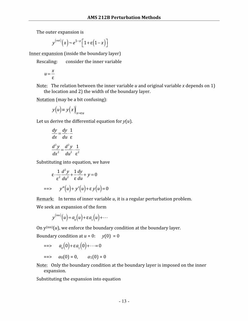
Theouterexpansionis
yout( ) x( )~e1−x 1+ ε 1− x( )⎡⎣ ⎤⎦
Innerexpansion(insidetheboundarylayer)Rescaling: considertheinnervariable
u= x
ε
Note: Therelationbetweentheinnervariableuandoriginalvariablexdependson1)thelocationand2)thewidthoftheboundarylayer.
Notation(maybeabitconfusing):
y u( )≡ y x( ) x=εu
Letusderivethedifferentialequationfory(u).
dydx
= dydu
⋅1ε
d2 ydx2
= d2 ydu2
⋅ 1ε2
Substitutingintoequation,wehave
ε⋅ 1ε2d2 ydu2
+ 1εdydu
+ y =0
==> ′′y u( )+ ′y u( )+ ε y u( ) =0 Remark: Intermsofinnervariableu,itisaregularperturbationproblem.Weseekanexpansionoftheform
yinn( ) u( ) = a0 u( )+ εa1 u( )+!
Ony(inn)(u),weenforcetheboundaryconditionattheboundarylayer.Boundaryconditionatu=0: y(0)=0
==> a0 0( )+ εa1 0( )+!=0
==> a0(0)=0, a1(0)=0
Note: Onlytheboundaryconditionattheboundarylayerisimposedontheinnerexpansion.
Substitutingtheexpansionintoequation
AMS212BPerturbationMethods
- 14 -
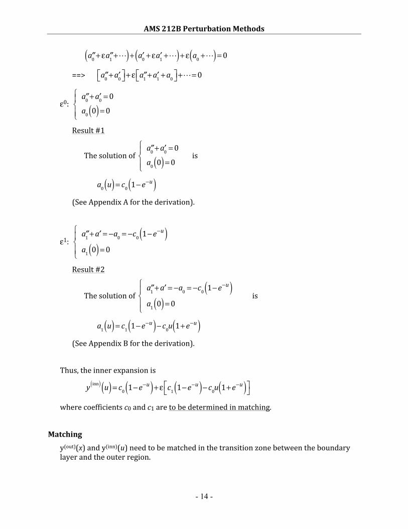
′′a0 + ε ′′a1 +!( )+ ′a0 + ε ′a1 +!( )+ ε a0 +!( ) =0 ==> ′′a0 + ′a0⎡⎣ ⎤⎦+ ε ′′a1 + ′a1 +a0⎡⎣ ⎤⎦+!=0
ε0:
′′a0 + ′a0 =0a0 0( ) =0
⎧⎨⎪
⎩⎪
Result#1
Thesolutionof
′′a0 + ′a0 =0a0 0( ) =0
⎧⎨⎪
⎩⎪ is
a0 u( ) = c0 1−e−u( ) (SeeAppendixAforthederivation).
ε1:
′′a1 + ′a = −a0 = −c0 1−e−u( )a1 0( ) =0
⎧⎨⎪
⎩⎪
Result#2
Thesolutionof
′′a1 + ′a = −a0 = −c0 1−e−u( )a1 0( ) =0
⎧⎨⎪
⎩⎪ is
a1 u( ) = c1 1−e−u( )− c0u 1+e−u( ) (SeeAppendixBforthederivation).
Thus,theinnerexpansionis
yinn( ) u( ) = c0 1−e−u( )+ ε c1 1−e−u( )− c0u 1+e−u( )⎡
⎣⎤⎦
wherecoefficientsc0andc1aretobedeterminedinmatching.
Matching
y(out)(x)andy(inn)(u)needtobematchedinthetransitionzonebetweentheboundarylayerandtheouterregion.
AMS212BPerturbationMethods
- 15 -
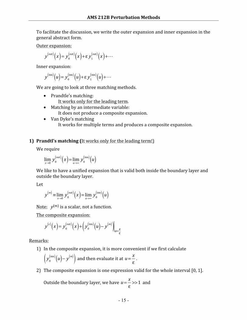
Tofacilitatethediscussion,wewritetheouterexpansionandinnerexpansioninthegeneralabstractform.Outerexpansion:
yout( ) x( ) = y0out( ) x( )+ ε y1out( ) x( )+!
Innerexpansion:
yinn( ) u( ) = y0inn( ) u( )+ ε y1inn( ) u( )+!
Wearegoingtolookatthreematchingmethods.
• Prandtle’smatching:Itworksonlyfortheleadingterm.
• Matchingbyanintermediatevariable:Itdoesnotproduceacompositeexpansion.
• VanDyke’smatchingItworksformultipletermsandproducesacompositeexpansion.
1) Prandtl’smatching(Itworksonlyfortheleadingterm!)
Werequire
limx→0y0out( ) x( ) = lim
u→∞y0inn( ) u( )
Weliketohaveaunifiedexpansionthatisvalidbothinsidetheboundarylayerandoutsidetheboundarylayer.Let
ym( ) ≡ lim
x→0y0out( ) x( ) = lim
u→∞y0inn( ) u( )
Note: y(m)isascalar,notafunction.
Thecompositeexpansion:
y c( ) x( ) = y0out( ) x( )+ y0
inn( ) u( )− y m( )( )u=xε
Remarks:1) Inthecompositeexpansion,itismoreconvenientifwefirstcalculate
y0inn( ) u( )− y m( )( ) andthenevaluateitat
u= x
ε.
2) Thecompositeexpansionisoneexpressionvalidforthewholeinterval[0,1].
Outsidetheboundarylayer,wehaveu= x
ε>>1 and
AMS212BPerturbationMethods
- 16 -
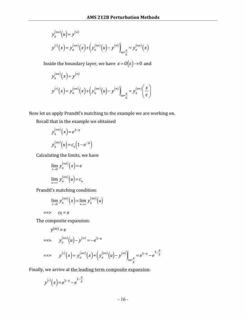
y0inn( ) u( )≈ y m( )
y c( ) x( ) = y0out( ) x( )+ y0
inn( ) u( )− y m( )( )u=xε
≈ y0out( ) x( )
Insidetheboundarylayer,wehavex =O ε( )→0 and
y0out( ) x( )≈ y m( )
y c( ) x( ) = y0out( ) x( )+ y0
inn( ) u( )− y m( )( )u=xε
≈ y0inn( ) x
ε⎛⎝⎜
⎞⎠⎟
NowletusapplyPrandtl’smatchingtotheexampleweareworkingon.
Recallthatintheexampleweobtained
y0out( ) x( ) = e1−x
y0inn( ) u( ) = c0 1−e−u( )
Calculatingthelimits,wehave
limx→0y0out( ) x( ) = e
limu→∞y0inn( ) u( ) = c0
Prandtl’smatchingcondition:
limx→0y0out( ) x( ) = lim
u→∞y0inn( ) u( )
==> c0=e
Thecompositeexpansion:
y(m)=e
==> y0inn( ) u( )− y m( ) = −e1−u
==>y c( ) x( ) = y0out( ) x( )+ y0
inn( ) u( )− y m( )( )u=xε
= e1−x −e1−xε
Finally,wearriveattheleadingtermcompositeexpansion:
yc( ) x( ) = e1−x −e1−
xε
AMS212BPerturbationMethods
- 17 -
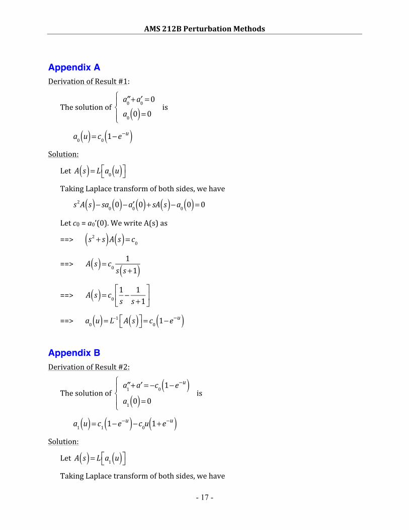
Appendix A DerivationofResult#1:
Thesolutionof
′′a0 + ′a0 =0a0 0( ) =0
⎧⎨⎪
⎩⎪is
a0 u( ) = c0 1−e−u( ) Solution:
LetA s( ) = L a0 u( )⎡⎣ ⎤⎦
TakingLaplacetransformofbothsides,wehave
s2A s( )− sa0 0( )− ′a0 0( )+ sA s( )−a0 0( ) =0
Letc0=a0’(0).WewriteA(s)as
==> s2 + s( )A s( ) = c0
==>A s( ) = c0 1
s s +1( )
==>A s( ) = c0 1
s− 1s +1
⎡
⎣⎢
⎤
⎦⎥
==> a0 u( ) = L−1 A s( )⎡⎣ ⎤⎦ = c0 1−e−u( )
Appendix B DerivationofResult#2:
Thesolutionof
′′a1 + ′a = −c0 1−e−u( )a1 0( ) =0
⎧⎨⎪
⎩⎪is
a1 u( ) = c1 1−e−u( )− c0u 1+e−u( ) Solution:
LetA s( ) = L a1 u( )⎡⎣ ⎤⎦
TakingLaplacetransformofbothsides,wehave
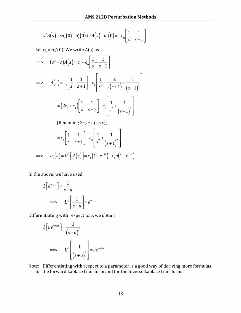
AMS212BPerturbationMethods
- 18 -
s2A s( )− sa1 0( )− ′a1 0( )+ sA s( )−a1 0( ) = −c0 1
s− 1s +1
⎡
⎣⎢
⎤
⎦⎥
Letc1=a1’(0).WewriteA(s)as
==>s2 + s( )A s( ) = c1 − c0 1
s− 1s +1
⎡
⎣⎢
⎤
⎦⎥
==>
A s( ) = c1 1
s− 1s +1
⎡
⎣⎢
⎤
⎦⎥− c0
1s2
− 2s s +1( ) +
1s +1( )2
⎡
⎣
⎢⎢⎢
⎤
⎦
⎥⎥⎥
= 2c0 + c1( ) 1s −
1s +1
⎡
⎣⎢
⎤
⎦⎥− c0
1s2
+ 1s +1( )2
⎡
⎣
⎢⎢⎢
⎤
⎦
⎥⎥⎥
(Renaming2c0+c1asc1)
= c1
1s− 1s +1
⎡
⎣⎢
⎤
⎦⎥− c0
1s2
+ 1s +1( )2
⎡
⎣
⎢⎢⎢
⎤
⎦
⎥⎥⎥
==> a1 u( ) = L−1 A s( )⎡⎣ ⎤⎦ = c1 1−e−u( )− c0u 1+e−u( )
Intheabove,wehaveused
L e−au⎡⎣ ⎤⎦ =
1s +a
==>L−1 1
s +a⎡
⎣⎢
⎤
⎦⎥ = e
−au
Differentiatingwithrespecttoa,weobtain
L ue−au⎡⎣ ⎤⎦ =
1s +a( )2
==>
L−1 1
s +a( )2⎡
⎣
⎢⎢⎢
⎤
⎦
⎥⎥⎥=ue−au
Note: DifferentiatingwithrespecttoaparameterisagoodwayofderivingmoreformulasfortheforwardLaplacetransformandfortheinverseLaplacetransform.