Amplitude Frequency Modulation - HP Memory Projecthpmemoryproject.org/an/pdf/an_150-1.pdfFrequency...

Test & MeasurementApplication Note 150-1

H

http://www.hp.com/go/tmappnotes

Spectrum Analysis

Amplitude&FrequencyModulation

http://www.hp.com/go/tmappnotes

HSpectrum Analysis 150-1Amplitude and Frequency Modulation

eAcos(ωt+φ )

=

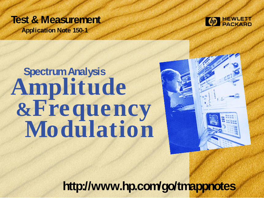
Chapter 1 – Modulation Methods

Chapter 2 – Amplitude Modulation Modulation Degree and Sideband Amplitude Zero Span and Markers The Fast Fourier Transform (FFT) Special Forms of Amplitude ModulationSingle Sideband

Chapter 3 – Angular Modulation Definitions Bandwidth of FM Signals FM Measurements with the Spectrum Analyzer AM Plus FM (Incidental FM)

Appendix A – Mathematics of Modulation

Appendix B – Frequency Modulation in Broadcast Radio

Relevant Products and Training

Contacting Hewlett-Packard Worldwide

ContentsSpectrum Analysis AM and FM

© Copyright Hewlett-Packard Company, 1989, 1996. 3000 Hanover Street, Palo Alto California, USA.2

3


Modulation is the act of translating some low-frequency or base-band signal (voice, music, data) to a higher frequency. Why do wemodulate signals? There are at least two reasons: to allow the simul-taneous transmission of two or more baseband signals by translatingthem to different frequencies, and to take advantage of the greaterefficiency and smaller size of higher-frequency antennas.

In the modulation process, some characteristic of a high-frequencysinusoidal carrier is changed in direct proportion to the instan-taneous amplitude of the baseband signal. The carrier itself can bedescribed by the equation

e(t) = A • cos (ωt + φ )where: A = peak amplitude of the carrier,

ω = angular frequency of the carrier in radians per second,t = time, andφ = initial phase of the carrier at time t = 0.

In the expression above there are two properties of the carrier thatcan be changed, the amplitude (A) and the angular position(argument of the cosine function). Thus we have amplitude mod-ulation and angular modulation. Angular modulation can be furthercharacterized as either frequency modulation or phase modulation.

1Modulation MethodsMilestones.

In 1864 James ClarkMaxwell predicted theexistence of electro-magnetic waves thattravel at the speed oflight. In Germany,Heinrich Hertz provedMaxwell's theory andin 1888 was the first tocreate electromagneticradio waves.

Amplitude modulation of a sine or cosine carrier results in avariation of the carrier amplitude that is proportional to theamplitude of the modulating signal. In the time domain(amplitude versus time), the amplitude modulation of onesinusoidal carrier by another sinusoid resembles Figure 1A.The mathematical expression for this complex wave showsthat it is the sum of three sinusoids of differentfrequencies.

One of these sinusoids has the same frequency andamplitude as the unmodulated carrier. The second sinusoidis at a frequency equal to the sum of the carrier frequencyand the modulation frequency; this component is the uppersideband. The third sinusoid is at a frequency equal to thecarrier frequency minus the modulation frequency; thiscomponent is the lower sideband. The two sidebandcomponents have equal amplitudes, which are proportionalto the amplitude of the modulating signal. Figure 1B showsthe carrier and sideband components of the amplitude-modulated wave of Figure 1A as they appear in thefrequency domain (amplitude versus frequency).

4

HSpectrum Analysis 150-1Amplitude and Frequency Modulation2Amplitude Modulation

Modulation Degree and Sideband AmplitudeFigure 1A.Time domain displayof an amplitude–modulated carrier.

Figure 1B.Frequency domain(spectrum analyzer)display of an amplitude-modulated carrier.

fcfc–fm fc+fm

USBLSB

Am

plitu

de

(Vo

lts)

t

Am

plitu

de

(Vo

lts)

5


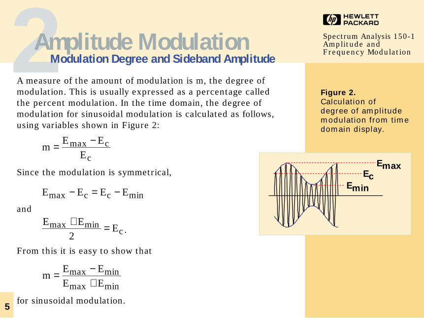
A measure of the amount of modulation is m, the degree ofmodulation. This is usually expressed as a percentage calledthe percent modulation. In the time domain, the degree ofmodulation for sinusoidal modulation is calculated as follows,using variables shown in Figure 2:

Since the modulation is symmetrical,

and

.

From this it is easy to show that

for sinusoidal modulation.

m

E EE E

= −+

max min

max min

E EEc

max min+ =2

E E E Ec cmax min− = −

m

E EE

c

c= −max

2Amplitude ModulationModulation Degree and Sideband Amplitude

Figure 2.

Calculation of degree of amplitudemodulation from timedomain display.

Emin

Ec

Emax

6


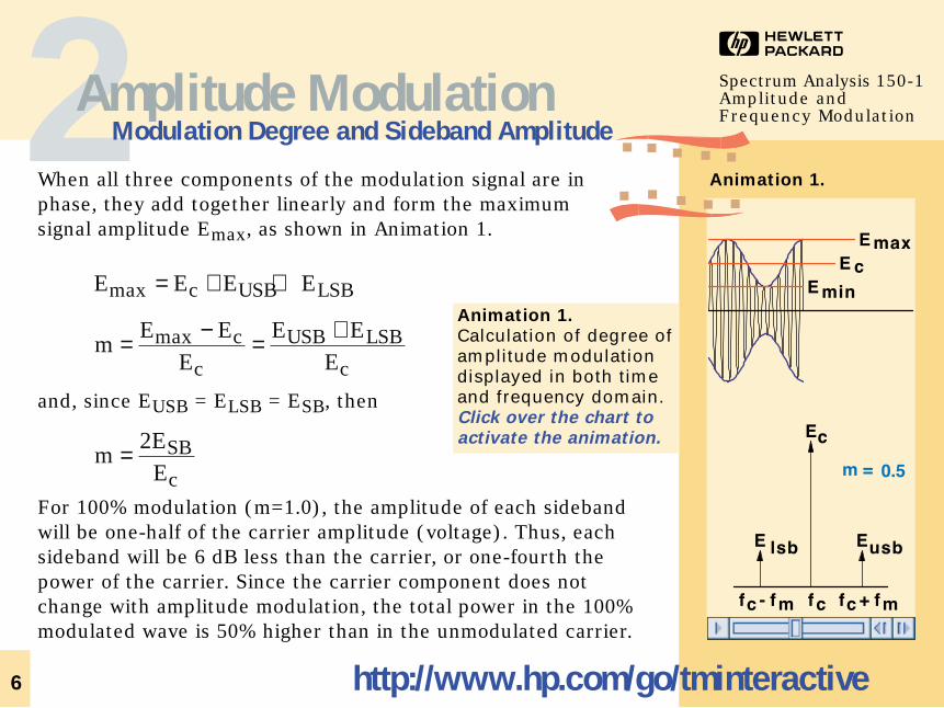
When all three components of the modulation signal are inphase, they add together linearly and form the maximum signal amplitude Emax, as shown in Animation 1.

and, since EUSB = ELSB = ESB, then

For 100% modulation (m=1.0), the amplitude of each sidebandwill be one-half of the carrier amplitude (voltage). Thus, eachsideband will be 6 dB less than the carrier, or one-fourth thepower of the carrier. Since the carrier component does notchange with amplitude modulation, the total power in the 100%modulated wave is 50% higher than in the unmodulated carrier.

m

EE

SB

c= 2

m

E EE

E EE

c

c

USB LSB

c= − = +max

E E E Ec USB LSBmax = + +


Animation 1.

Calculation of degree ofamplitude modulationdisplayed in both timeand frequency domain.Click over the chart toactivate the animation.

http://www.hp.com/go/tminteractive

Animation 1.

f cf - f c m f + f c m

Ec

E lsb Eusb

m = 0.5

E min

E c

E max


7


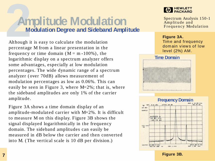
Although it is easy to calculate the modulationpercentage M from a linear presentation in thefrequency or time domain (M = m •100%), thelogarithmic display on a spectrum analyzer offerssome advantages, especially at low modulationpercentages. The wide dynamic range of a spectrumanalyzer (over 70dB) allows measurement ofmodulation percentages as low as 0.06%. This caneasily be seen in Figure 3, where M=2%; that is, wherethe sideband amplitudes are only 1% of the carrieramplitude.

Figure 3A shows a time domain display of anamplitude-modulated carrier with M=2%. It is difficultto measure M on this display. Figure 3B shows thesignal displayed logarithmically in the frequencydomain. The sideband amplitudes can easily bemeasured in dB below the carrier and then convertedinto M. (The vertical scale is 10 dB per division.)


Figure 3A.

Time and frequencydomain views of lowlevel (2%) AM.

Time Domain

Frequency Domain

Figure 3B.

M%


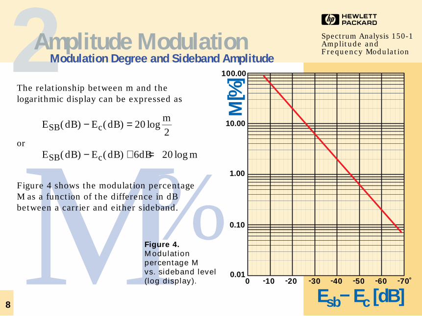
The relationship between m and thelogarithmic display can be expressed as

or

Figure 4 shows the modulation percentageM as a function of the difference in dBbetween a carrier and either sideband.

E dB E dB dB mSB c( ) ( ) log− + =6 20

E dB E dB

mSB c( ) ( ) log− = 20

2


0 -10 -20 -30 -40 -70 0.01

0.10

1.00

10.00

100.00

-50 -60

M[ %

]

Esb– Ec [dB]

Figure 4.

Modulationpercentage M vs. sideband level(log display).

8

9


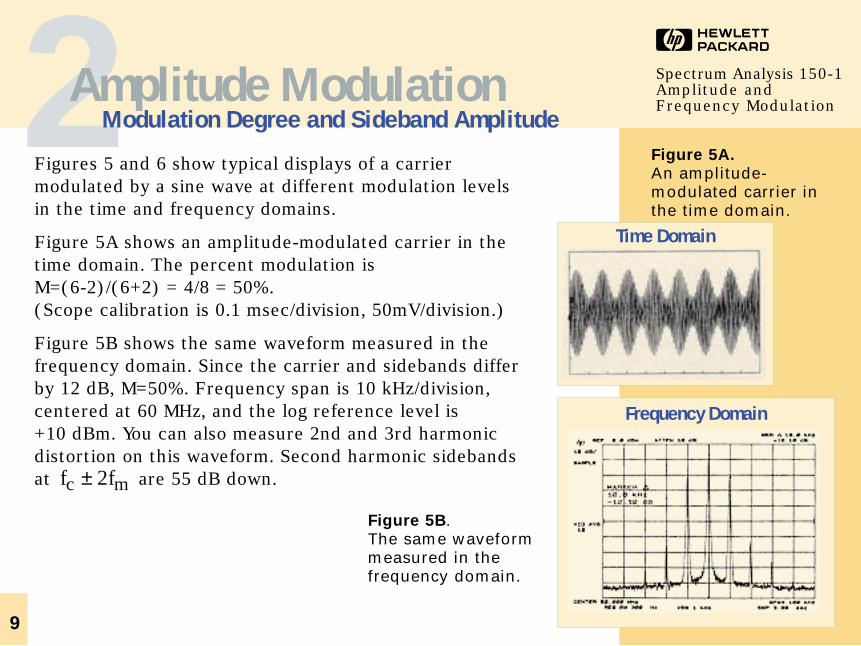
Figures 5 and 6 show typical displays of a carriermodulated by a sine wave at different modulation levelsin the time and frequency domains.

Figure 5A shows an amplitude-modulated carrier in the time domain. The percent modulation is M=(6-2)/(6+2) = 4/8 = 50%. (Scope calibration is 0.1 msec/division, 50mV/division.)

Figure 5B shows the same waveform measured in thefrequency domain. Since the carrier and sidebands differby 12 dB, M=50%. Frequency span is 10 kHz/division,centered at 60 MHz, and the log reference level is +10 dBm. You can also measure 2nd and 3rd harmonicdistortion on this waveform. Second harmonic sidebandsat are 55 dB down. f fc m± 2


Figure 5A.

An amplitude-modulated carrier inthe time domain.

Time Domain

Frequency Domain

Figure 5B. The same waveformmeasured in thefrequency domain.

10

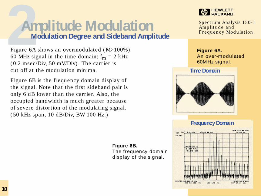
Figure 6A shows an overmodulated (M>100%)60 MHz signal in the time domain; fm = 2 kHz(0.2 msec/Div, 50 mV/Div). The carrier is cut off at the modulation minima.

Figure 6B is the frequency domain display ofthe signal. Note that the first sideband pair isonly 6 dB lower than the carrier. Also, theoccupied bandwidth is much greater becauseof severe distortion of the modulating signal.(50 kHz span, 10 dB/Div, BW 100 Hz.)


Modulation Degree and Sideband Amplitude

Figure 6B.

The frequency domaindisplay of the signal.

Figure 6A.

An over-modulated60MHz signal.

Time Domain

Frequency Domain

http://www.hp.com/go/tminteractive11


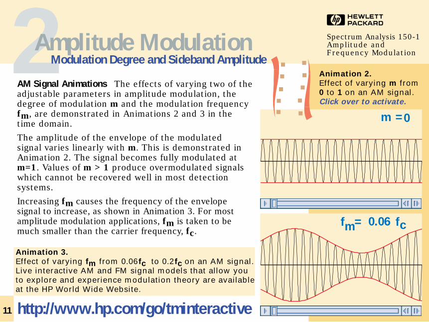
AM Signal Animations The effects of varying two of theadjustable parameters in amplitude modulation, thedegree of modulation m and the modulation frequencyfm, are demonstrated in Animations 2 and 3 in thetime domain.

The amplitude of the envelope of the modulatedsignal varies linearly with m. This is demonstrated inAnimation 2. The signal becomes fully modulated atm=1. Values of m > 1 produce overmodulated signalswhich cannot be recovered well in most detectionsystems.

Increasing fm causes the frequency of the envelopesignal to increase, as shown in Animation 3. For mostamplitude modulation applications, fm is taken to bemuch smaller than the carrier frequency, fc.


m =0

f =m 0.06 fc

Animation 2.

Effect of varying m from0 to 1 on an AM signal.Click over to activate.

Animation 3.

Effect of varying fm from 0.06 fc to 0.2 fc on an AM signal.Live interactive AM and FM signal models that allow you to explore and experience modulation theory are availableat the HP World Wide Website.


12


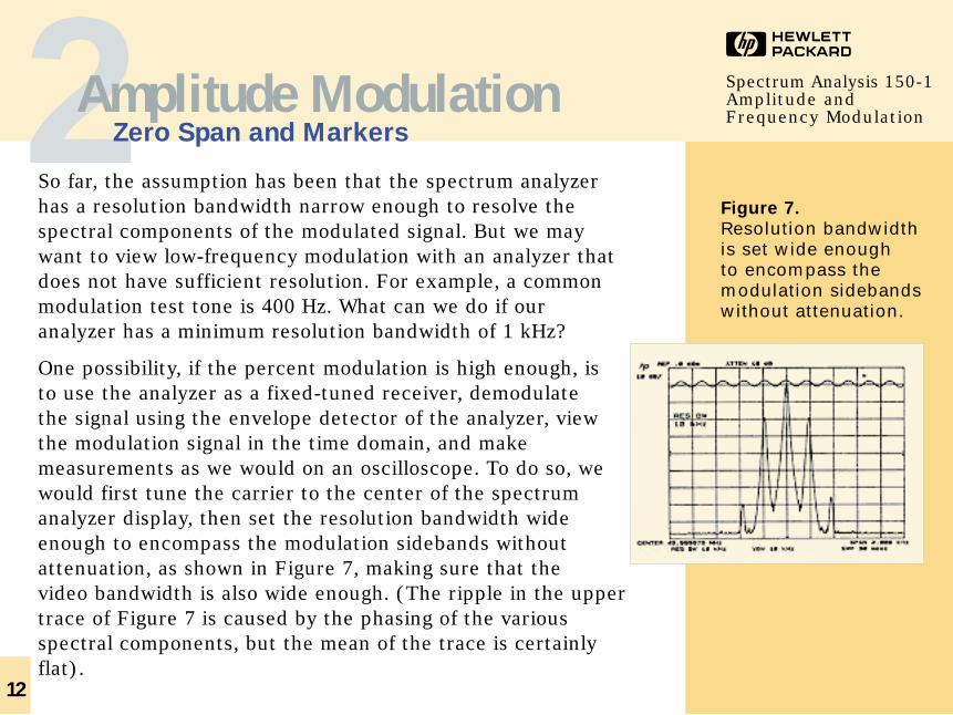
So far, the assumption has been that the spectrum analyzerhas a resolution bandwidth narrow enough to resolve thespectral components of the modulated signal. But we maywant to view low-frequency modulation with an analyzer thatdoes not have sufficient resolution. For example, a commonmodulation test tone is 400 Hz. What can we do if ouranalyzer has a minimum resolution bandwidth of 1 kHz?

One possibility, if the percent modulation is high enough, isto use the analyzer as a fixed-tuned receiver, demodulatethe signal using the envelope detector of the analyzer, viewthe modulation signal in the time domain, and makemeasurements as we would on an oscilloscope. To do so, wewould first tune the carrier to the center of the spectrumanalyzer display, then set the resolution bandwidth wideenough to encompass the modulation sidebands withoutattenuation, as shown in Figure 7, making sure that thevideo bandwidth is also wide enough. (The ripple in the uppertrace of Figure 7 is caused by the phasing of the variousspectral components, but the mean of the trace is certainlyflat).

2Amplitude ModulationZero Span and Markers

Figure 7.

Resolution bandwidthis set wide enough to encompass themodulation sidebandswithout attenuation.

13


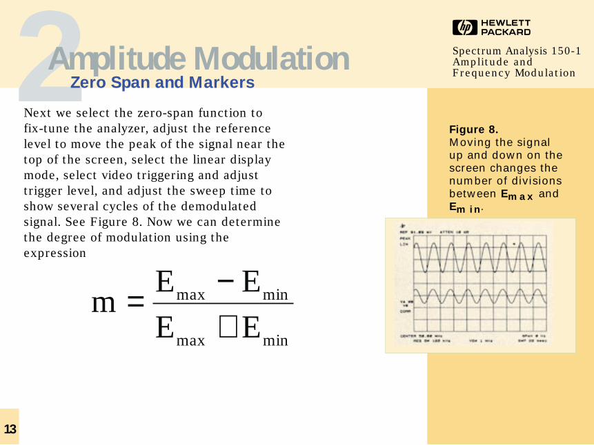
Next we select the zero-span function to fix-tune the analyzer, adjust the referencelevel to move the peak of the signal near thetop of the screen, select the linear displaymode, select video triggering and adjusttrigger level, and adjust the sweep time toshow several cycles of the demodulatedsignal. See Figure 8. Now we can determinethe degree of modulation using theexpression


Figure 8.

Moving the signal up and down on thescreen changes thenumber of divisionsbetween Em a x andEm i n.

m

E E

E E= −

+max min

max min

14


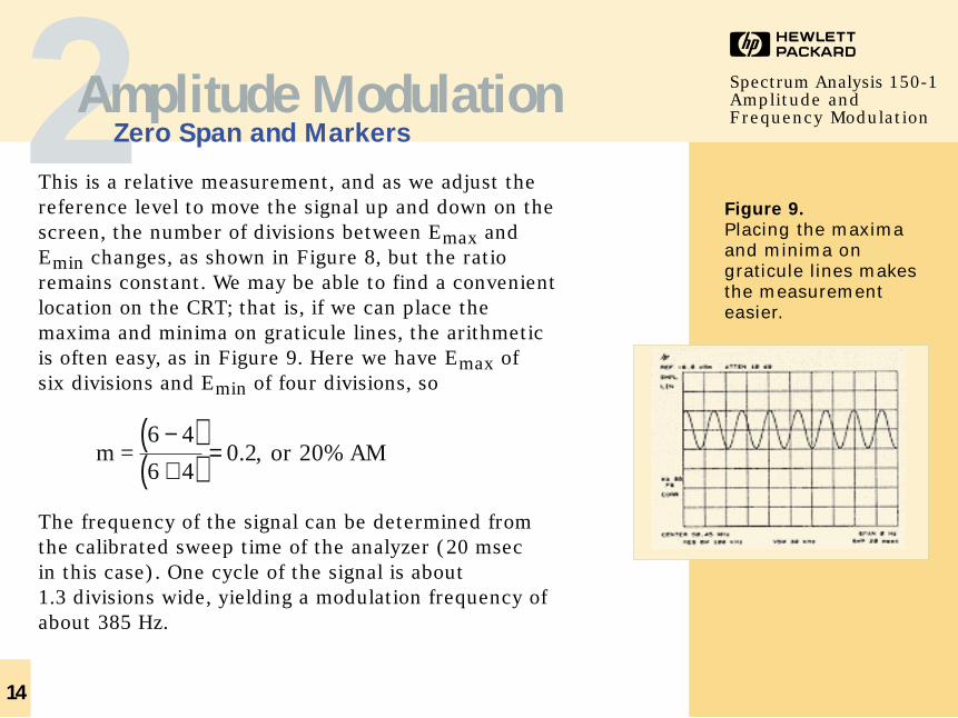
This is a relative measurement, and as we adjust thereference level to move the signal up and down on thescreen, the number of divisions between Emax andEmin changes, as shown in Figure 8, but the ratioremains constant. We may be able to find a convenientlocation on the CRT; that is, if we can place themaxima and minima on graticule lines, the arithmeticis often easy, as in Figure 9. Here we have Emax of six divisions and Emin of four divisions, so

The frequency of the signal can be determined fromthe calibrated sweep time of the analyzer (20 msec in this case). One cycle of the signal is about 1.3 divisions wide, yielding a modulation frequency ofabout 385 Hz.

m =

6

−( )+( ) =

4

6 40 2 20. , %or AM


Figure 9.

Placing the maximaand minima ongraticule lines makesthe measurementeasier.

15


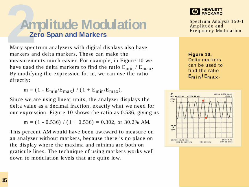
Many spectrum analyzers with digital displays also havemarkers and delta markers. These can make themeasurements much easier. For example, in Figure 10 wehave used the delta markers to find the ratio Emin / Emax. By modifying the expression for m, we can use the ratiodirectly:

m = (1 - Emin/Emax) / (1 + Emin/Emax).

Since we are using linear units, the analyzer displays thedelta value as a decimal fraction, exactly what we need forour expression. Figure 10 shows the ratio as 0.536, giving us

m = (1 - 0.536) / (1 + 0.536) = 0.302, or 30.2% AM.

This percent AM would have been awkward to measure onan analyzer without markers, because there is no place onthe display where the maxima and minima are both ongraticule lines. The technique of using markers works welldown to modulation levels that are quite low.


Figure 10.

Delta markerscan be used tofind the ratioEm i n /Em a x .

16

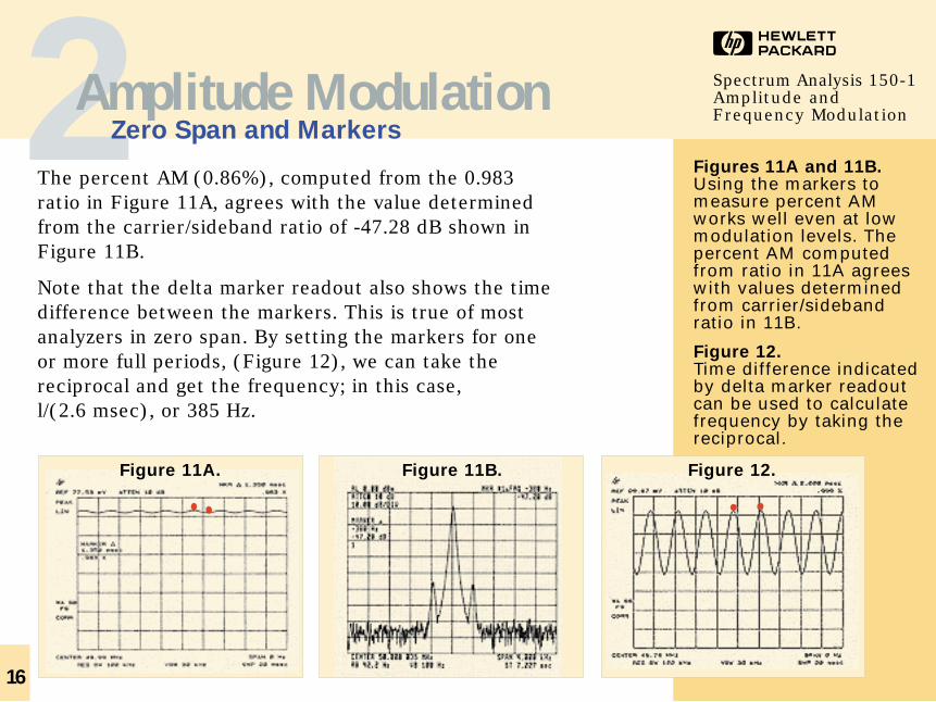
The percent AM (0.86%), computed from the 0.983ratio in Figure 11A, agrees with the value determinedfrom the carrier/sideband ratio of -47.28 dB shown inFigure 11B.

Note that the delta marker readout also shows the timedifference between the markers. This is true of mostanalyzers in zero span. By setting the markers for oneor more full periods, (Figure 12), we can take thereciprocal and get the frequency; in this case, l/(2.6 msec), or 385 Hz.


Zero Span and Markers

Figure 12.Figure 11A. Figure 11B.

Figures 11A and 11B.Using the markers tomeasure percent AMworks well even at lowmodulation levels. Thepercent AM computedfrom ratio in 11A agreeswith values determinedfrom carrier/sidebandratio in 11B.

Figure 12.Time difference indicatedby delta marker readoutcan be used to calculatefrequency by taking thereciprocal.

17


There is an even easier way to make the measurements above ifthe analyzer has the ability to perform an FFT on the demodulatedsignal. On the HP 8590 and HP 8560 portable spectrum analyzers,FFT is available on a soft key. On the HP 8566B, 8567A, 8568B and71000 series spectrum analyzers, FFT is available in ROM, and wecan write a DLP (down-loadable program) to take advantage of it.

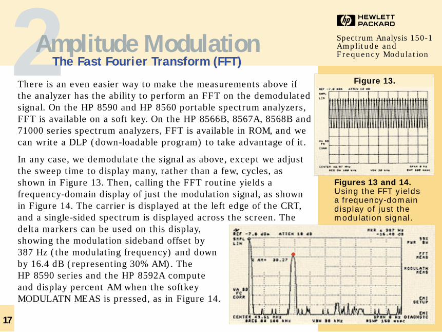
In any case, we demodulate the signal as above, except we adjustthe sweep time to display many, rather than a few, cycles, as shown in Figure 13. Then, calling the FFT routine yields afrequency-domain display of just the modulation signal, as shown in Figure 14. The carrier is displayed at the left edge of the CRT,and a single-sided spectrum is displayed across the screen. Thedelta markers can be used on this display,showing the modulation sideband offset by 387 Hz (the modulating frequency) and downby 16.4 dB (representing 30% AM). The HP 8590 series and the HP 8592A compute and display percent AM when the softkeyMODULATN MEAS is pressed, as in Figure 14.

2Amplitude ModulationThe Fast Fourier Transform (FFT)

Figures 13 and 14.Using the FFT yields a frequency-domaindisplay of just themodulation signal.

Figure 13.

18


FFT capability is particularly useful for measuringdistortion. Figure 15 shows our demodulated signal at60% AM level. It is impossible to determine themodulation distortion from this display. The FFTdisplay in Figure 16, on the other hand, indicatesabout 0.5% second-harmonic distortion.

The maximum modulating frequency for which theFFT can be used on a spectrum analyzer is a functionof the rate at which the data are sampled (digitized);that is, it’s directly proportional to the number of datapoints across the CRT and inversely proportional tothe sweep time.


Figure 16.

An FFT displayindicates themodulation distortion;in this case, about0.5% second-harmonicdistortion.

Figure 15.

The modulationdistortion of our signalcannot be read fromthis display.

19


For the HP 8566B, 8567A, and 8568B, the maximumfrequency (right edge of the CRT) is 25 kHz; for theHP 8590 and HP 8560 portable series, it is 10 kHz;for the HP 71000 series, it’s 10 kHz.

Note that lower frequencies can be measured: verylow frequencies, in fact. With a 20-second sweep,the HP 8566B, 8567A, and 8568B can measure downto 0.5 Hz.

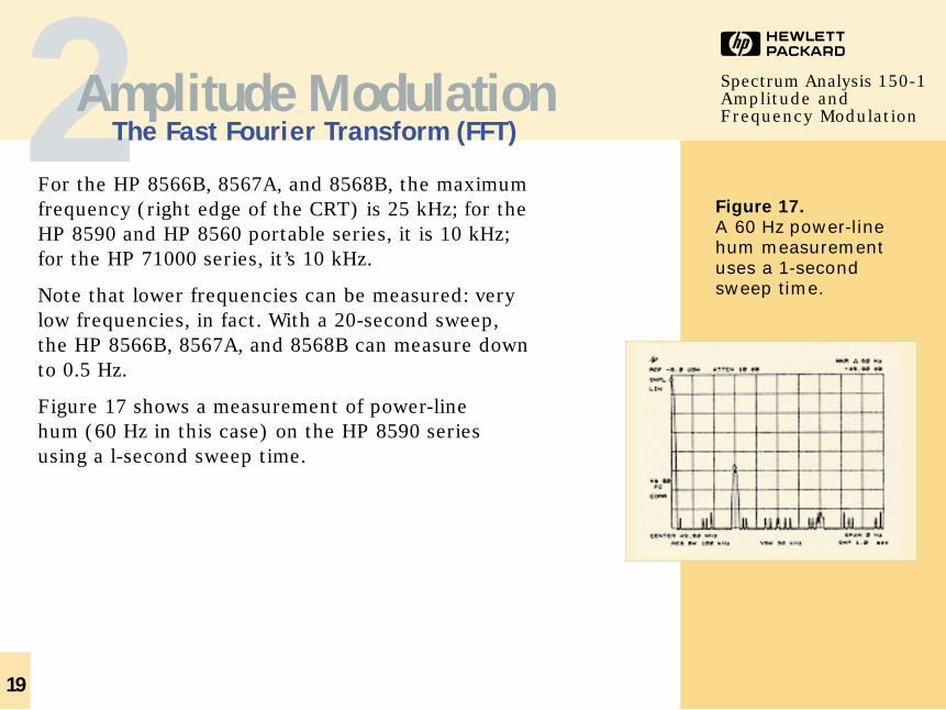
Figure 17 shows a measurement of power-linehum (60 Hz in this case) on the HP 8590 seriesusing a l-second sweep time.


Figure 17.

A 60 Hz power-linehum measurementuses a 1-secondsweep time.

20


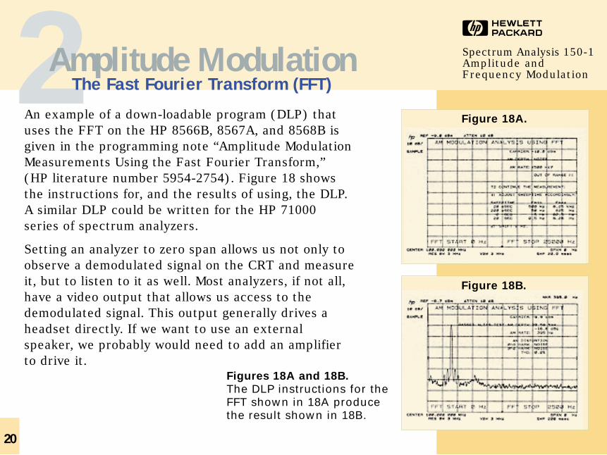
An example of a down-loadable program (DLP) thatuses the FFT on the HP 8566B, 8567A, and 8568B isgiven in the programming note “Amplitude ModulationMeasurements Using the Fast Fourier Transform,” (HP literature number 5954-2754). Figure 18 showsthe instructions for, and the results of using, the DLP.A similar DLP could be written for the HP 71000series of spectrum analyzers.

Setting an analyzer to zero span allows us not only toobserve a demodulated signal on the CRT and measureit, but to listen to it as well. Most analyzers, if not all,have a video output that allows us access to thedemodulated signal. This output generally drives aheadset directly. If we want to use an externalspeaker, we probably would need to add an amplifierto drive it.


Figures 18A and 18B.

The DLP instructions for theFFT shown in 18A producethe result shown in 18B.

Figure 18A.

Figure 18B.

21


Many analyzers include an AM demodulator and aninternal speaker so that we can listen to signalswithout external hardware. As a convenience, someanalyzers provide a marker pause function so we neednot even be in zero span to hear the signals.

To use this feature, we set the frequency spanto cover the desired range (that is, the AMbroadcast band), set the active marker on thesignal of interest, set the length of the pause(dwell time), and activate the AM demodulator.The analyzer then sweeps to the marker andpauses for the set time, allowing us to listen tothe signal for that interval, before completingthe sweep. If the marker is the active function,we can move it, and thus listen to any othersignal on the display.


Milestones.

In 1895 GuglielmoMarconi of Italy madethe first radio forcommunicating withships at sea. In 1901Marconi sent the firstsignal across theAtlantic.

22


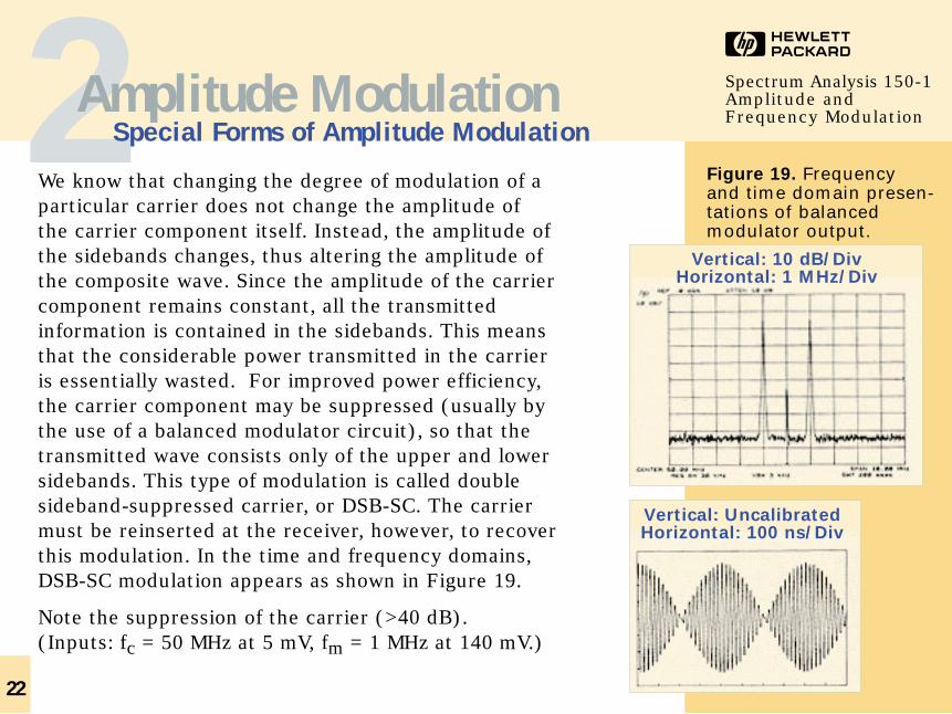
We know that changing the degree of modulation of aparticular carrier does not change the amplitude ofthe carrier component itself. Instead, the amplitude ofthe sidebands changes, thus altering the amplitude ofthe composite wave. Since the amplitude of the carriercomponent remains constant, all the transmittedinformation is contained in the sidebands. This meansthat the considerable power transmitted in the carrieris essentially wasted. For improved power efficiency,the carrier component may be suppressed (usually bythe use of a balanced modulator circuit), so that thetransmitted wave consists only of the upper and lowersidebands. This type of modulation is called doublesideband-suppressed carrier, or DSB-SC. The carriermust be reinserted at the receiver, however, to recoverthis modulation. In the time and frequency domains,DSB-SC modulation appears as shown in Figure 19.

Note the suppression of the carrier (>40 dB). (Inputs: fc = 50 MHz at 5 mV, fm = 1 MHz at 140 mV.)

2Amplitude ModulationSpecial Forms of Amplitude Modulation

Figure 19. Frequency and time domain presen-tations of balancedmodulator output.

Vertical: 10 dB/DivHorizontal: 1 MHz/Div

Vertical: UncalibratedHorizontal: 100 ns/Div

23


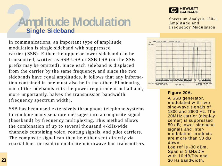
In communications, an important type of amplitudemodulation is single sideband with suppressed carrier (SSB). Either the upper or lower sideband can betransmitted, written as SSB-USB or SSB-LSB (or the SSBprefix may be omitted). Since each sideband is displacedfrom the carrier by the same frequency, and since the twosidebands have equal amplitudes, it follows that any informa-tion contained in one must also be in the other. Eliminatingone of the sidebands cuts the power requirement in half and,more importantly, halves the transmission bandwidth(frequency spectrum width).

SSB has been used extensively throughout telephone systemsto combine many separate messages into a composite signal(baseband) by frequency multiplexing. This method allowsthe combination of up to several thousand 4-kHz-widechannels containing voice, routing signals, and pilot carriers.The composite signal can then be either sent directly viacoaxial lines or used to modulate microwave line transmitters.

2Amplitude ModulationSingle Sideband

Figure 20A.

A SSB generator,modulated with twosine-wave signals of1800 and 2600 Hz. The20MHz carrier (displaycenter) is suppressed50 dB; lower sidebandsignals and inter-modulation productsare more than 50 dBdown.Log ref is -30 dBm.Span is 1 kHz/Div with 10 dB/Div and 30 Hz bandwidth.

24


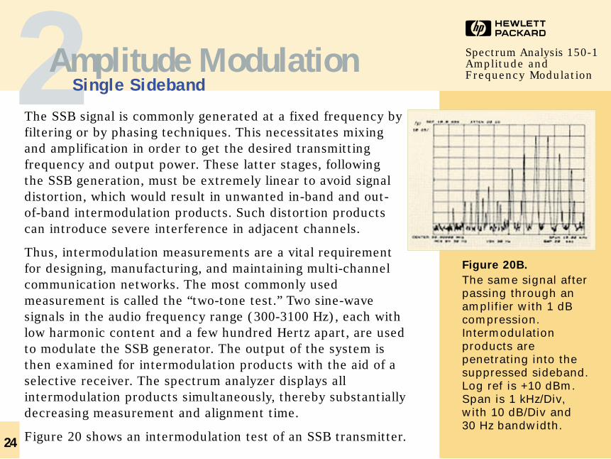
The SSB signal is commonly generated at a fixed frequency byfiltering or by phasing techniques. This necessitates mixingand amplification in order to get the desired transmittingfrequency and output power. These latter stages, followingthe SSB generation, must be extremely linear to avoid signaldistortion, which would result in unwanted in-band and out-of-band intermodulation products. Such distortion productscan introduce severe interference in adjacent channels.

Thus, intermodulation measurements are a vital requirement for designing, manufacturing, and maintaining multi-channelcommunication networks. The most commonly usedmeasurement is called the “two-tone test.” Two sine-wavesignals in the audio frequency range (300-3100 Hz), each withlow harmonic content and a few hundred Hertz apart, are usedto modulate the SSB generator. The output of the system isthen examined for intermodulation products with the aid of aselective receiver. The spectrum analyzer displays allintermodulation products simultaneously, thereby substantiallydecreasing measurement and alignment time.

Figure 20 shows an intermodulation test of an SSB transmitter.

2Amplitude ModulationSingle Sideband

Figure 20B.

The same signal afterpassing through anamplifier with 1 dBcompression.Intermodulationproducts arepenetrating into thesuppressed sideband.Log ref is +10 dBm.Span is 1 kHz/Div,with 10 dB/Div and 30 Hz bandwidth.

25

HSpectrum Analysis 150-1Amplitude and Frequency Modulation3Angular Modulation

Definitions

In Chapter 1 we described a carrier as

e(t) = A • cos (ωt + φ )and, in addition, stated that angular modulation can becharacterized as either frequency or phase modulation.In either case, we think of a constant carrier plus orminus some incremental change.

Frequency Modulation

The instantaneous frequency deviation of the modulatedcarrier with respect to the frequency of the unmodulatedcarrier is directly proportional to the instantaneousamplitude of the modulating signal.

Phase Modulation

The instantaneous phase deviation of the modulatedcarrier with respect to the phase of the unmodulatedcarrier is directly proportional to the instantaneousamplitude of the modulating signal.

Milestone.

The Superheterodyneradio circuit, inventedby E.H. Armstrong in1918, did much toimprove radio receiversand circuits. In 1933Armstrong inventedFrequency Modulation,known today as FM.

26


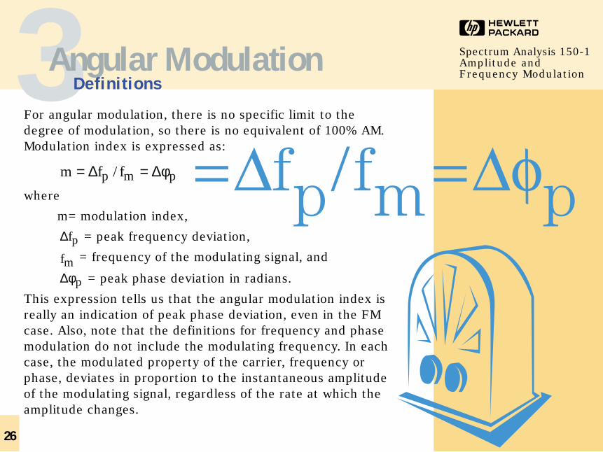
For angular modulation, there is no specific limit to thedegree of modulation, so there is no equivalent of 100% AM.Modulation index is expressed as:

where

m= modulation index,

= peak frequency deviation,

= frequency of the modulating signal, and

= peak phase deviation in radians.

This expression tells us that the angular modulation index isreally an indication of peak phase deviation, even in the FMcase. Also, note that the definitions for frequency and phasemodulation do not include the modulating frequency. In eachcase, the modulated property of the carrier, frequency orphase, deviates in proportion to the instantaneous amplitudeof the modulating signal, regardless of the rate at which theamplitude changes.

∆φp

fm

∆fp

m f fp m p= =∆ ∆/ φ

3Angular ModulationDefinitions

27


However, the frequency of the modulating signal is important inFM. In the expression for the modulating index, it is the ratio ofpeak frequency deviation to modulation frequency that equates tophase. Comparing this basic equation with the two definitions ofmodulation, we find

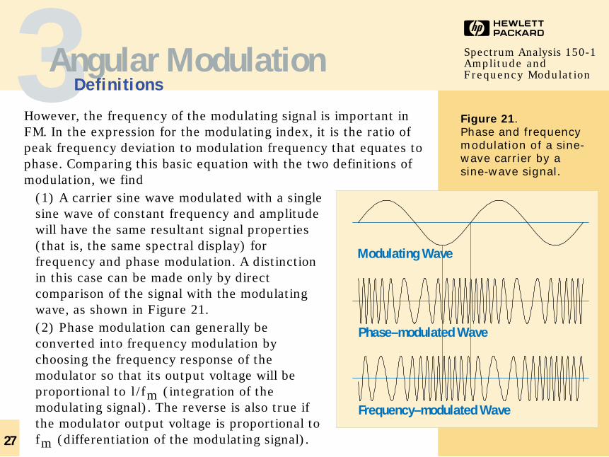
(1) A carrier sine wave modulated with a singlesine wave of constant frequency and amplitudewill have the same resultant signal properties(that is, the same spectral display) forfrequency and phase modulation. A distinctionin this case can be made only by directcomparison of the signal with the modulatingwave, as shown in Figure 21.(2) Phase modulation can generally beconverted into frequency modulation bychoosing the frequency response of themodulator so that its output voltage will beproportional to l / fm (integration of themodulating signal). The reverse is also true ifthe modulator output voltage is proportional tofm (differentiation of the modulating signal).

Figure 21. Phase and frequencymodulation of a sine-wave carrier by asine-wave signal.

Modulating Wave

Phase–modulated Wave

Frequency–modulated Wave


Because phase modulation can be applied at the amplifierstage of a transmitter, a very stable crystal-controlledoscillator can be used. Thus, “indirect FM” is commonlyused in VHF and UHF communication stations wherehighly stable carrier frequencies are required.

We can see that the amplitude of the modulated signalalways remains constant, regardless of modulation frequencyand amplitude. The modulating signal adds no power to thecarrier in angular modulation as it does with amplitude modulation.

Mathematical treatment shows that, in contrast to amplitudemodulation, angular modulation of a sine-wave carrier with a singlesine wave yields an infinite number of sidebands spaced by themodulation frequency, fm . In other words, AM is a linear process,whereas FM is a nonlinear process. For distortion-free detection ofthe modulating signal, all sidebands must be transmitted. Thespectral components (including the carrier component) changetheir amplitudes when the modulation index m is varied. The sumof the squares of these components always yields a compositesignal with an average power that remains constant and equal tothe average power of the unmodulated carrier wave.28


Definitions

Milestones.

There are more than10,000 AM and FMradio stations in theUnited States, morethan anywhere else inthe world.It is estimated that30,000 radio stationsoperate outside theUnited States.

29


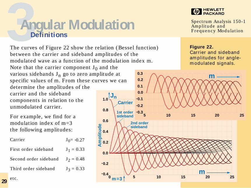
The curves of Figure 22 show the relation (Bessel function)between the carrier and sideband amplitudes of themodulated wave as a function of the modulation index m.Note that the carrier component J0 and thevarious sidebands Jn go to zero amplitude atspecific values of m. From these curves we candetermine the amplitudes of thecarrier and the sidebandcomponents in relation to theunmodulated carrier.

For example, we find for amodulation index of m=3 the following amplitudes:

Carrier J0= -0.27

First order sideband J1 = 0.33

Second order sideband J2 = 0.48

Third order sideband J3 = 0.33

etc.


Figure 22.

Carrier and sidebandamplitudes for angle-modulated signals.

0 5 10 15 20 25-0.4

-0.2

0.0

0.2

0.4

0.6

0.8

1.0Carrier

JnA

mp

litu

de

m=3

1st order sideband

2nd order sideband

5 10 15 20 25-0.3

-0.2

-0.1

0.0

0.1

0.2

0.3m

m

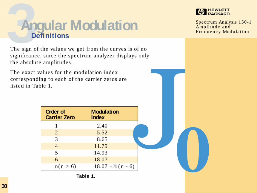
The sign of the values we get from the curves is of nosignificance, since the spectrum analyzer displays onlythe absolute amplitudes.

The exact values for the modulation indexcorresponding to each of the carrier zeros arelisted in Table 1.

Order of ModulationCarrier Zero Index

1 2.40 2 5.52 3 8.65 4 11.79 5 14.93 6 18.07 n(n > 6) 18.07 +π (n - 6)

30


Definitions

Table 1.

31


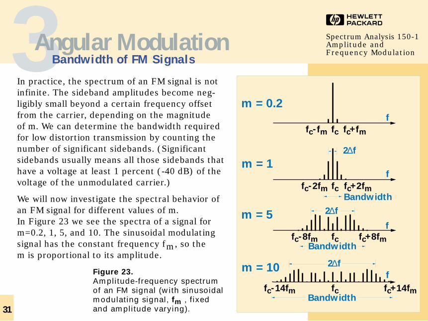
In practice, the spectrum of an FM signal is notinfinite. The sideband amplitudes become neg-ligibly small beyond a certain frequency offsetfrom the carrier, depending on the magnitude of m. We can determine the bandwidth requiredfor low distortion transmission by counting thenumber of significant sidebands. (Significantsidebands usually means all those sidebands thathave a voltage at least 1 percent (-40 dB) of thevoltage of the unmodulated carrier.)

We will now investigate the spectral behavior ofan FM signal for different values of m. In Figure 23 we see the spectra of a signal for m=0.2, 1, 5, and 10. The sinusoidal modulatingsignal has the constant frequency fm , so the m is proportional to its amplitude.

3Angular ModulationBandwidth of FM Signals

Figure 23.

Amplitude-frequency spectrumof an FM signal (with sinusoidalmodulating signal, fm , fixedand amplitude varying).

fc

fc

fc

fcfc- fm

fc-2fm

fc-8fm

fc-14fm

fc+fm

fc+2fm

fc+8fm

fc+14fm

2∆f

2∆f

2∆f

Bandwidth

Bandwidth

Bandwidth

f

f

f

f

m = 0.2

m = 1

m = 5

m = 10

32


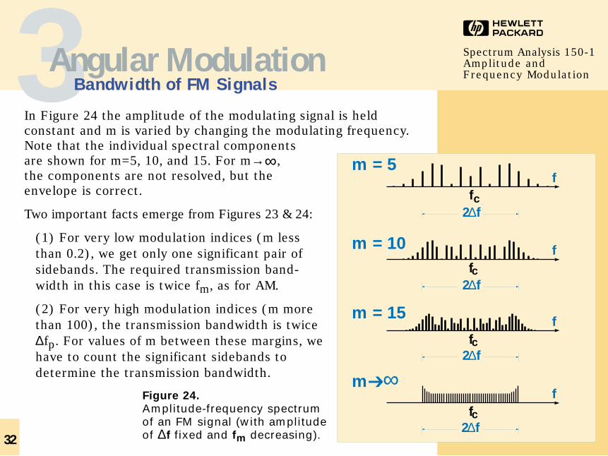
In Figure 24 the amplitude of the modulating signal is heldconstant and m is varied by changing the modulating frequency.Note that the individual spectral components are shown for m=5, 10, and 15. For m→ ∞ , the components are not resolved, but theenvelope is correct.

Two important facts emerge from Figures 23 & 24:

(1) For very low modulation indices (m lessthan 0.2), we get only one significant pair ofsidebands. The required transmission band-width in this case is twice fm, as for AM.

(2) For very high modulation indices (m morethan 100), the transmission bandwidth is twice∆fp. For values of m between these margins, wehave to count the significant sidebands todetermine the transmission bandwidth.


m = 5

m = 10

m = 15

fc

fc

fc

f

f

f

f

2∆f

2∆f

2∆f

2∆f

fc

m➔∞Figure 24.

Amplitude-frequency spectrumof an FM signal (with amplitudeof ∆f fixed and fm decreasing).

33


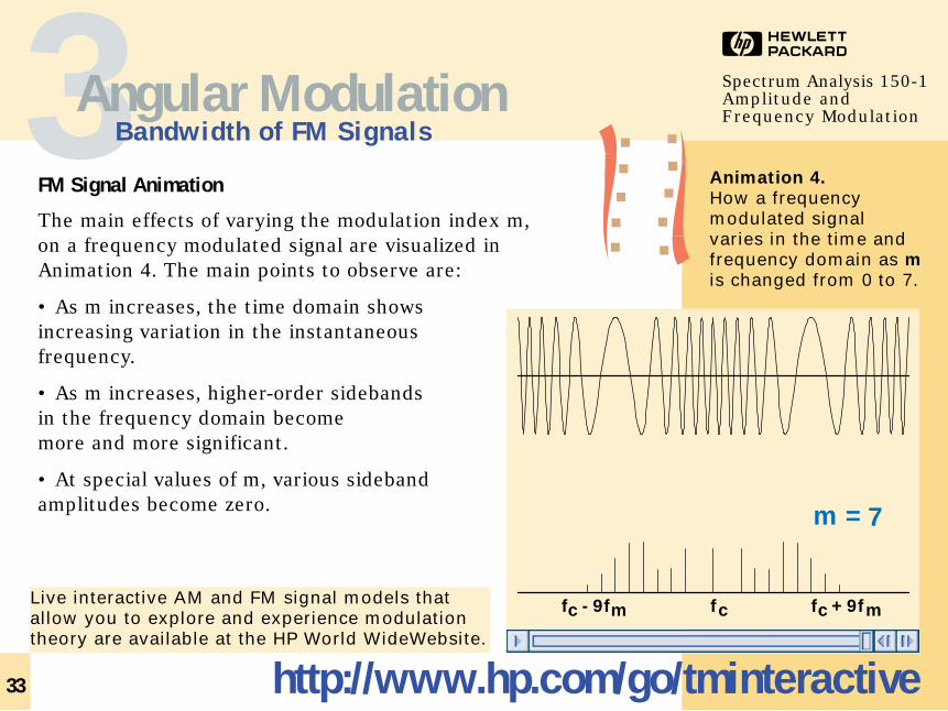
FM Signal Animation

The main effects of varying the modulation index m,on a frequency modulated signal are visualized inAnimation 4. The main points to observe are:

• As m increases, the time domain showsincreasing variation in the instantaneousfrequency.

• As m increases, higher-order sidebandsin the frequency domain becomemore and more significant.

• At special values of m, various sidebandamplitudes become zero.


Animation 4.

How a frequencymodulated signalvaries in the time andfrequency domain as mis changed from 0 to 7.

c m fcf - 9f f + 9f c m

m = 7

Live interactive AM and FM signal models thatallow you to explore and experience modulationtheory are available at the HP World WideWebsite.



34


Bandwidth of FM Signals

Figure 25, 26. Sinusoidalmodulating signals.

0 2 4 6 8 10 12 14m

16

Ban

dw

idth

/∆

f

1

2

3

4

5

6

7

8

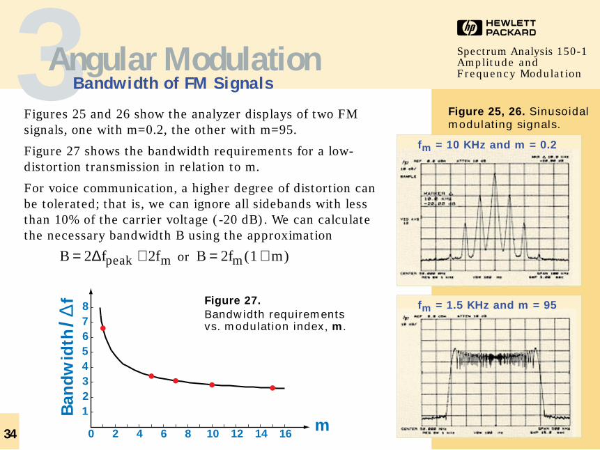
Figures 25 and 26 show the analyzer displays of two FMsignals, one with m=0.2, the other with m=95.

Figure 27 shows the bandwidth requirements for a low-distortion transmission in relation to m.

For voice communication, a higher degree of distortion canbe tolerated; that is, we can ignore all sidebands with lessthan 10% of the carrier voltage (-20 dB). We can calculatethe necessary bandwidth B using the approximation

or B f mm= +2 1( ) B f fpeak m= +2 2∆

Figure 27.

Bandwidth requirementsvs. modulation index, m.

fm = 10 KHz and m = 0.2

fm = 1.5 KHz and m = 95

35


Bandwidth of FM Signals

So far, our discussion of FM sidebands and bandwidth hasbeen based on having a single sine wave as the modulatingsignal. Extending the discussion to complex and more realisticmodulating signals is difficult. We can, however, look at anexample of single-tone modulation for some usefulinformation.

An FM broadcast station has a maximum frequency deviation(determined by the maximum amplitude of the modulatingsignal) of ∆fpeak = 75 kHz. The highest modulation frequency,fm , is 15 kHz. This yields a modulation index of m = 5, andthe resulting signal has eight significant sideband pairs. Thusthe required bandwidth can be calculated as 2 x 8 x 15 kHz =240 kHz. For modulation frequencies below 15 kHz (with thesame amplitude assumed), the modulation index increasesabove 5, with the bandwidth eventually approaching 2 ∆fpeak = 150 kHz for very low modulation frequencies.

We can, therefore, calculate the required transmissionbandwidth using the highest modulation frequency and themaximum frequency deviation ∆fpeak.

36


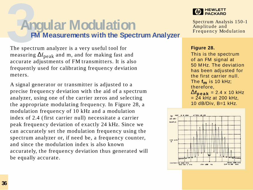
The spectrum analyzer is a very useful tool formeasuring ∆fpeak and m, and for making fast andaccurate adjustments of FM transmitters. It is alsofrequently used for calibrating frequency deviationmeters.

A signal generator or transmitter is adjusted to aprecise frequency deviation with the aid of a spectrumanalyzer, using one of the carrier zeros and selectingthe appropriate modulating frequency. In Figure 28, amodulation frequency of 10 kHz and a modulationindex of 2.4 (first carrier null) necessitate a carrierpeak frequency deviation of exactly 24 kHz. Since wecan accurately set the modulation frequency using thespectrum analyzer or, if need be, a frequency counter,and since the modulation index is also knownaccurately, the frequency deviation thus generated willbe equally accurate.

3Angular ModulationFM Measurements with the Spectrum Analyzer

Figure 28.

This is the spectrum of an FM signal at 50 MHz. The deviationhas been adjusted forthe first carrier null.The fm is 10 kHz;therefore,∆fp e a k = 2.4 x 10 kHz= 24 kHz at 200 kHz, 10 dB/Div, B=1 kHz.

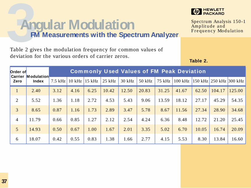
Table 2 gives the modulation frequency for common values ofdeviation for the various orders of carrier zeros.

Order of Commonly Used Values of FM Peak DeviationCarrier Modulation

Zero Index 7.5 kHz 10 kHz 15 kHz 25 kHz 30 kHz 50 kHz 75 kHz 100 kHz 150 kHz 250 kHz 300 kHz

1 2.40 3.12 4.16 6.25 10.42 12.50 20.83 31.25 41.67 62.50 104.17 125.00

2 5.52 1.36 1.18 2.72 4.53 5.43 9.06 13.59 18.12 27.17 45.29 54.35

3 8.65 0.87 1.16 1.73 2.89 3.47 5.78 8.67 11.56 27.34 28.90 34.68

4 11.79 0.66 0.85 1.27 2.12 2.54 4.24 6.36 8.48 12.72 21.20 25.45

5 14.93 0.50 0.67 1.00 1.67 2.01 3.35 5.02 6.70 10.05 16.74 20.09

6 18.07 0.42 0.55 0.83 1.38 1.66 2.77 4.15 5.53 8.30 13.84 16.60

37


FM Measurements with the Spectrum Analyzer

Table 2.

38


The procedure for setting up a known deviation is:

(1) Select the column with the required deviation: for example,250 kHz.

(2) Select an order of carrier zero that gives a frequency in thetable commensurate with the normal modulation bandwidth ofthe generator to be tested. For example, if 250 kHz was chosento test an audio modulation circuit, it will be necessary to go tothe fifth carrier zero to get a modulating frequency within theaudio pass-band of the generator (here, 16.74 kHz).

(3) Set the modulating frequency to 16.74 kHz, and monitor theoutput spectrum of the generator on the spectrum analyzer.Adjust the amplitude of the audio modulating signal until thecarrier amplitude has gone through four zeros; stop when thecarrier is at its fifth minimum. With a modulating frequency of16.74 kHz and the spectrum at its fifth zero, the setup provides a unique 250 kHz deviation. The modulation meter can then becalibrated. Make a quick check by moving to the adjacent carrierzero and resetting the modulating frequency and amplitude (inthis case, resetting to 13.84 kHz at the sixth carrier zero).


39


Other intermediate deviations and modulation indexes can beset using different orders of sideband zeros, but these areinfluenced by incidental amplitude modulation. Since weknow that amplitude modulation does not cause the carrierto change, but instead puts all the modulation power intothe sidebands, incidental AM will not affect the carrierzero method described on the previous page.

If it is not possible or desirable to alter the modulationfrequency to get a carrier or sideband null, there are otherways to obtain usable information about frequency deviationand modulation index. One method is to calculate m by usingthe amplitude information of five adjacent frequencycomponents in the FM signal. These five measurements areused in a recursion formula for Bessel functions to form threecalculated values of a modulation index. Averaging them yieldsa value for m that takes practical measurement errors intoconsideration. Because of the number of calculations necessary,this method is feasible only by using a computer. A somewhateasier method consists of the following two measurements.


Milestones.

In 1931 a stereophonic sound system was invented by A.D. Blumlein. It wasnot until 1982 that A.M.radio stations in theUnited States beganbroadcasting in stereo.

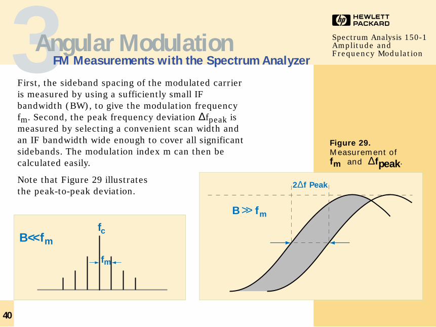
First, the sideband spacing of the modulated carrieris measured by using a sufficiently small IFbandwidth (BW), to give the modulation frequencyfm. Second, the peak frequency deviation ∆fpeak ismeasured by selecting a convenient scan width andan IF bandwidth wide enough to cover all significantsidebands. The modulation index m can then becalculated easily.

Note that Figure 29 illustrates the peak-to-peak deviation.

40



Figure 29.

Measurement offm and ∆fpeak.

2∆f Peak

B f m>> fc

fm

B << f m

41


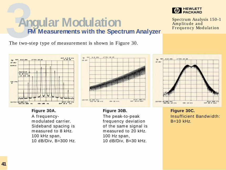
The two-step type of measurement is shown in Figure 30.


Figure 30A.

A frequency-modulated carrier.Sideband spacing ismeasured to 8 kHz.100 kHz span, 10 dB/Div, B=300 Hz.

Figure 30B.

The peak-to-peakfrequency deviationof the same signal ismeasured to 20 kHz.100 Hz span, 10 dB/Div, B=30 kHz.

Figure 30C.

Insufficient Bandwidth:B=10 kHz.

42


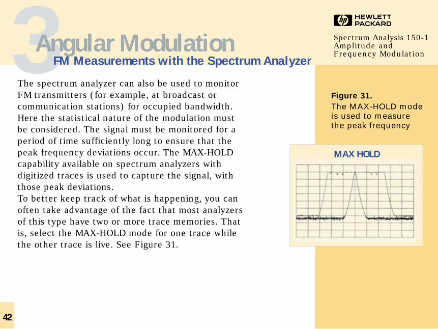
The spectrum analyzer can also be used to monitorFM transmitters (for example, at broadcast orcommunication stations) for occupied bandwidth.Here the statistical nature of the modulation mustbe considered. The signal must be monitored for aperiod of time sufficiently long to ensure that thepeak frequency deviations occur. The MAX-HOLDcapability available on spectrum analyzers withdigitized traces is used to capture the signal, withthose peak deviations. To better keep track of what is happening, you canoften take advantage of the fact that most analyzersof this type have two or more trace memories. Thatis, select the MAX-HOLD mode for one trace whilethe other trace is live. See Figure 31.


Figure 31.

The MAX-HOLD modeis used to measurethe peak frequency

MAX HOLD

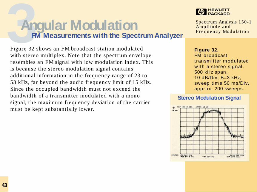
Figure 32 shows an FM broadcast station modulatedwith stereo multiplex. Note that the spectrum enveloperesembles an FM signal with low modulation index. Thisis because the stereo modulation signal containsadditional information in the frequency range of 23 to53 kHz, far beyond the audio frequency limit of 15 kHz.Since the occupied bandwidth must not exceed thebandwidth of a transmitter modulated with a monosignal, the maximum frequency deviation of the carriermust be kept substantially lower.

43



Figure 32.

FM broadcasttransmitter modulatedwith a stereo signal.500 kHz span, 10 dB/Div, B=3 kHz,sweep time 50 ms/Div,approx. 200 sweeps.

Stereo Modulation Signal

44


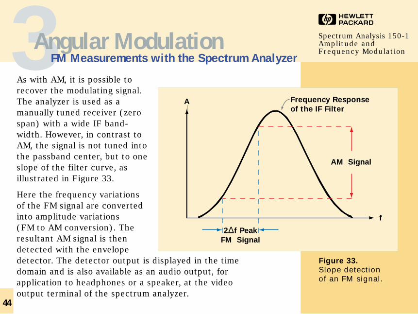
As with AM, it is possible torecover the modulating signal.The analyzer is used as amanually tuned receiver (zerospan) with a wide IF band-width. However, in contrast toAM, the signal is not tuned intothe passband center, but to oneslope of the filter curve, asillustrated in Figure 33.

Here the frequency variationsof the FM signal are convertedinto amplitude variations (FM to AM conversion). Theresultant AM signal is thendetected with the envelopedetector. The detector output is displayed in the timedomain and is also available as an audio output, forapplication to headphones or a speaker, at the videooutput terminal of the spectrum analyzer.


Figure 33.

Slope detectionof an FM signal.

A

f

Frequency Response

of the IF Filter

AM Signal

2∆f Peak

FM Signal

45


A disadvantage of this method is that the detector alsoresponds to amplitude variations of the signal. Many of today’sspectrum analyzers include an FM demodulator in addition tothe AM demodulator. Therefore, we can again take advantageof the marker pause function to listen to an FM broadcastwhile in the swept-frequency mode.

We would set the frequency span to cover the desired range(that is, the FM broadcast band); set the active marker on thesignal of interest, set the length of the pause (dwell time);and activate the FM demodulator. The analyzer sweeps to themarker and pauses for the set time, allowing us to listen tothe signal during that pause interval. After the pause interval,the analyzer continues the sweep. If the marker is the activefunction, we can move it and listen to any other signal on the display.


46


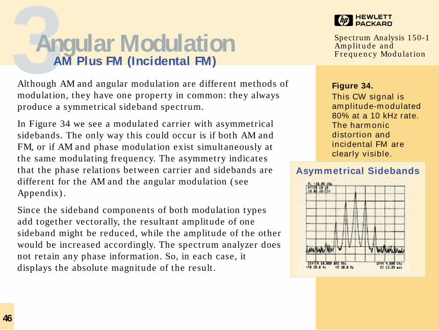
Although AM and angular modulation are different methods ofmodulation, they have one property in common: they alwaysproduce a symmetrical sideband spectrum.

In Figure 34 we see a modulated carrier with asymmetricalsidebands. The only way this could occur is if both AM andFM, or if AM and phase modulation exist simultaneously atthe same modulating frequency. The asymmetry indicatesthat the phase relations between carrier and sidebands aredifferent for the AM and the angular modulation (seeAppendix).

Since the sideband components of both modulation typesadd together vectorally, the resultant amplitude of onesideband might be reduced, while the amplitude of the otherwould be increased accordingly. The spectrum analyzer doesnot retain any phase information. So, in each case, itdisplays the absolute magnitude of the result.

3Angular ModulationAM Plus FM (Incidental FM)

Asymmetrical Sidebands

Figure 34.

This CW signal isamplitude-modulated80% at a 10 kHz rate.The harmonicdistortion andincidental FM areclearly visible.

47


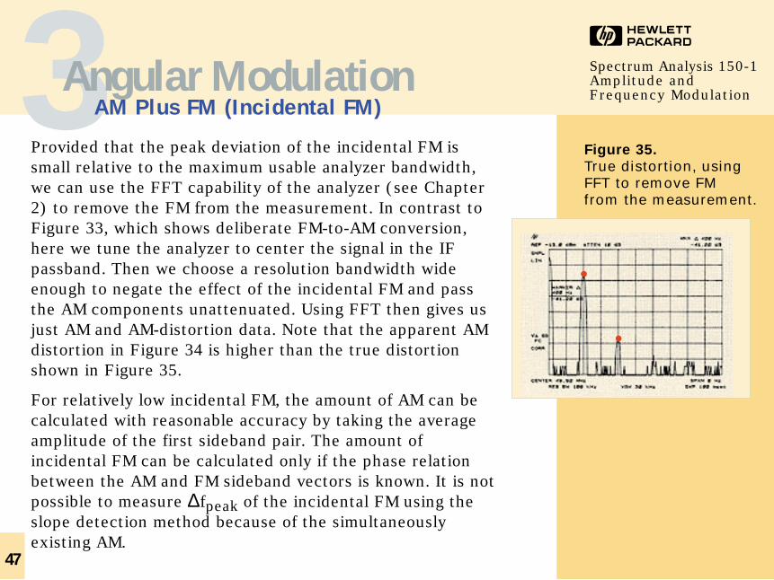
Provided that the peak deviation of the incidental FM issmall relative to the maximum usable analyzer bandwidth,we can use the FFT capability of the analyzer (see Chapter2) to remove the FM from the measurement. In contrast toFigure 33, which shows deliberate FM-to-AM conversion,here we tune the analyzer to center the signal in the IFpassband. Then we choose a resolution bandwidth wideenough to negate the effect of the incidental FM and passthe AM components unattenuated. Using FFT then gives usjust AM and AM-distortion data. Note that the apparent AMdistortion in Figure 34 is higher than the true distortionshown in Figure 35.

For relatively low incidental FM, the amount of AM can becalculated with reasonable accuracy by taking the averageamplitude of the first sideband pair. The amount ofincidental FM can be calculated only if the phase relationbetween the AM and FM sideband vectors is known. It is notpossible to measure ∆fpeak of the incidental FM using theslope detection method because of the simultaneouslyexisting AM.

3Angular ModulationAM Plus FM (Incidental FM)

Figure 35.

True distortion, usingFFT to remove FMfrom the measurement.

eAcos(ωt+φ )

=

48

HSpectrum Analysis 150-1Amplitude and Frequency ModulationAMathematics of Modulation

Amplitude Modulation

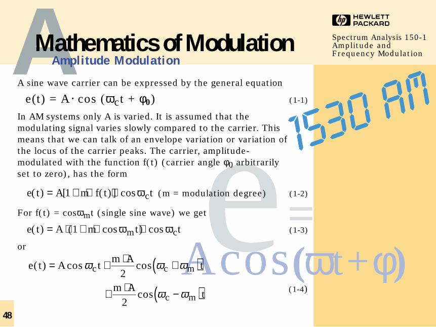
A sine wave carrier can be expressed by the general equation

e(t) = A • cos (ωct + φ 0) (1-1)

In AM systems only A is varied. It is assumed that themodulating signal varies slowly compared to the carrier. Thismeans that we can talk of an envelope variation or variation ofthe locus of the carrier peaks. The carrier, amplitude-modulated with the function f(t) (carrier angle φ 0 arbitrarilyset to zero), has the form

(m = modulation degree) (1-2)

For f(t) = cosωmt (single sine wave) we get

(1-3)

or

(1-4)

e t A m t tm c( ) ( cos ) cos= ⋅ + ⋅ ⋅1 ω ω

e t A m f t tc( ) [ ( )] cos= + ⋅ ⋅1 ω

e t A tm A

t

m At

c c m

c m

( ) cos cos

cos

= + ⋅ +( )

+ ⋅ −( )

ω ω ω

ω ω

2

2

49


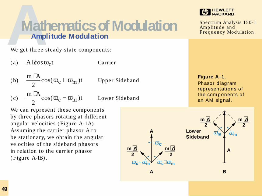
We get three steady-state components:

(a) Carrier

(b) Upper Sideband

(c) Lower Sideband

We can represent these components by three phasors rotating at differentangular velocities (Figure A-1A).Assuming the carrier phasor A to be stationary, we obtain the angularvelocities of the sideband phasors in relation to the carrier phasor (Figure A-lB).

m Atc m

⋅ −2

cos( )ω ω

m Atc m

⋅ +2

cos( )ω ω

A tc⋅cosω

AMathematics of ModulationAmplitude Modulation

Lower

Sideband

A

A

A

B

2⋅m A

2⋅m A

2⋅m A

2⋅m A

c m−ω ω c+ω mω

cωmω mω

Figure A–1.

Phasor diagramrepresentations ofthe components ofan AM signal.

50


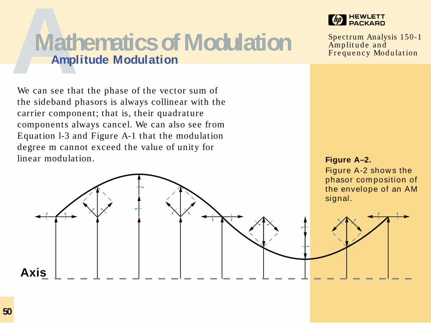
We can see that the phase of the vector sum ofthe sideband phasors is always collinear with thecarrier component; that is, their quadraturecomponents always cancel. We can also see fromEquation l-3 and Figure A-1 that the modulationdegree m cannot exceed the value of unity forlinear modulation.

AMathematics of ModulationAmplitude Modulation

Axis

Figure A–2.

Figure A-2 shows thephasor composition ofthe envelope of an AMsignal.

51


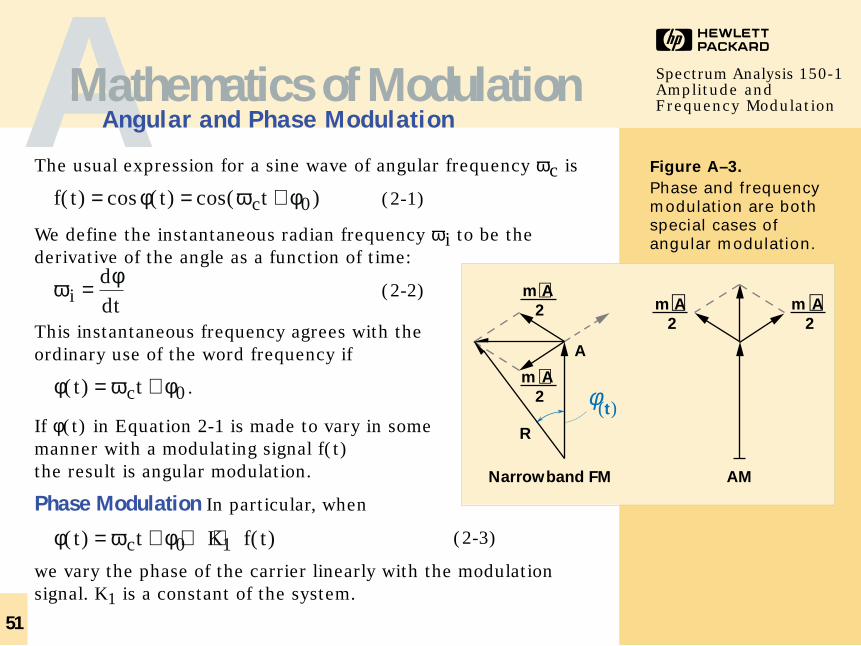
The usual expression for a sine wave of angular frequency ωc is

(2-1)

We define the instantaneous radian frequency ωi to be thederivative of the angle as a function of time:

(2-2)

This instantaneous frequency agrees with theordinary use of the word frequency if

.

If φ (t) in Equation 2-1 is made to vary in somemanner with a modulating signal f(t) the result is angular modulation.

Phase Modulation In particular, when

(2-3)

we vary the phase of the carrier linearly with the modulationsignal. K1 is a constant of the system.

φ ω φ( ) ( )t t K f tc= + + ⋅0 1

φ ω φ( )t tc= + 0

ω φ

iddt

=

f t t tc( ) cos ( ) cos( )= = +φ ω φ0

AMathematics of ModulationAngular and Phase Modulation

A

Narrowband FM

R

AM

2⋅m A

2⋅m A

2⋅m A

2⋅m A

φ( )t

Figure A–3.

Phase and frequencymodulation are bothspecial cases ofangular modulation.

52


Now we let the instantaneous frequency, as defined in Equation 2-2, vary linearly with the modulating signal

Then

(2-4)

In the case of phase modulation, the phase of the carrier varieswith the modulation signal, and in the case of FM the phase of thecarrier varies with the integral of the modulating signal. Thus,there is no essential difference between phase and frequencymodulation. We shall use the term FM generally to include bothmodulation types. For further analysis we assume a sinusoidalmodulation signal at the frequency fm:

The instantaneous radian frequency ωi is

(2-5)

∆ωpeak is a constant depending on the amplitude, a, of themodulating signal and on the properties of the modulating system.

ω ω ω ω ω ωi c peak m peak ct= + ⋅ <<∆ ∆cos ,

f t a tm( ) cos= ⋅ ω

φ ω ω φ( ) ( ) ( )t t dt t K f t dtc= = + + ⋅∫ ∫0 2

ω ω( ) ( )t K f tc= + ⋅2

AMathematics of ModulationFrequency Modulation

53


The phase φ (t) is then

We can take φ 0 as zero by referring to an appropriate phasereference. The frequency modulated carrier is then expressedby

(2-6)

For

(2-7)

In frequency modulation, m is the modulation index andrepresents the maximum phase shift of the carrier; ∆fpeak isthe maximum frequency deviation of the carrier.

m

f

fpeak

m

peak

m= =

∆ ∆ωω

e t A t m tc m( ) cos( sin )= ⋅ + ⋅ω ω

φ ω ω

ωω

ω φ( ) sint dt t ti cpeak

mm= = + +∫

∆0

AMathematics of ModulationFrequency Modulation

54


To simplify the analysis of FM, we first assume that (usually m < 0.2). We have

for

and ,

thus

(2-8)

Written in sideband form

(2-9)

e t A t m t tc m c( ) (cos sin sin )= ⋅ − ⋅ ⋅ω ω ω

sin( sin ) sinm t m tm m⋅ = ⋅ω ω cos( sin )m tm⋅ =ω 1 m << π

2

m << π

2

AMathematics of ModulationNarrowband FM

e t A t m t

A t m t t m t

c m

c m c m

( ) cos( sin )

cos cos sin sin sin sin

= ⋅ + ⋅

= ⋅ ⋅( ) − ⋅ ⋅( )[ ]ω ω

ω ω ω ω

e t A tm A

t

m At

c c m

c m

( ) cos cos( )

cos( ) .

= + ⋅ +

− ⋅ −

ω ω ω

ω ω

2

2

55


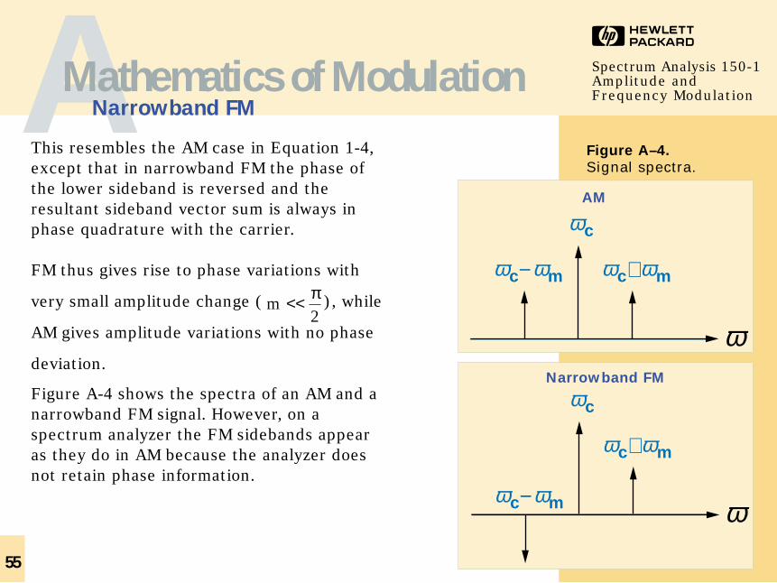
This resembles the AM case in Equation 1-4,except that in narrowband FM the phase ofthe lower sideband is reversed and theresultant sideband vector sum is always inphase quadrature with the carrier.

FM thus gives rise to phase variations with

very small amplitude change ( ), while

AM gives amplitude variations with no phase

deviation.

Figure A-4 shows the spectra of an AM and anarrowband FM signal. However, on aspectrum analyzer the FM sidebands appearas they do in AM because the analyzer doesnot retain phase information.

m << π

2

AMathematics of ModulationNarrowband FM

Figure A–4.

Signal spectra.

ωc m−ω ω

c+ω mω

cωNarrowband FM

c m−ω ω c+ω mω

cω

ω

AM

56


Wideband FM

e tJ m t J m t t

J m t tJ m t t

c c m c m

c m c m

c m c m

( )( ) cos ( )[cos( ) cos( ) ]

( )[cos( ) cos( ) ]( )[cos( ) cos( ) ]

...

=⋅ − − − +

+ − + +− − − ++

0 1

2

3

2 23 3

ω ω ω ω ωω ω ω ωω ω ω ω

For m not small

Using the Fourier series expansion,

(2-10)

(2-11)When Jn(m) is the nth-order Bessel function of the first kind, we get

(2-12)

sin( sin ) ( ) sin

( ) sin ...

m t J m t

J m tm m

m

⋅ = ⋅+ ⋅ +

ω ωω

2

2 31

3

cos( sin )

( ) ( ) cos ( ) cos ...

m t

J m J m t J m tm

m m

⋅ =+ ⋅ + ⋅ +

ωω ω0 2 42 2 2 4

= ⋅ ⋅ ⋅ − ⋅ ⋅A t m t t m tc m c m[cos cos( sin ) sin sin( sin )]ω ω ω ω e t A t m tc m( ) cos( sin )= ⋅ + ⋅ω ω

57


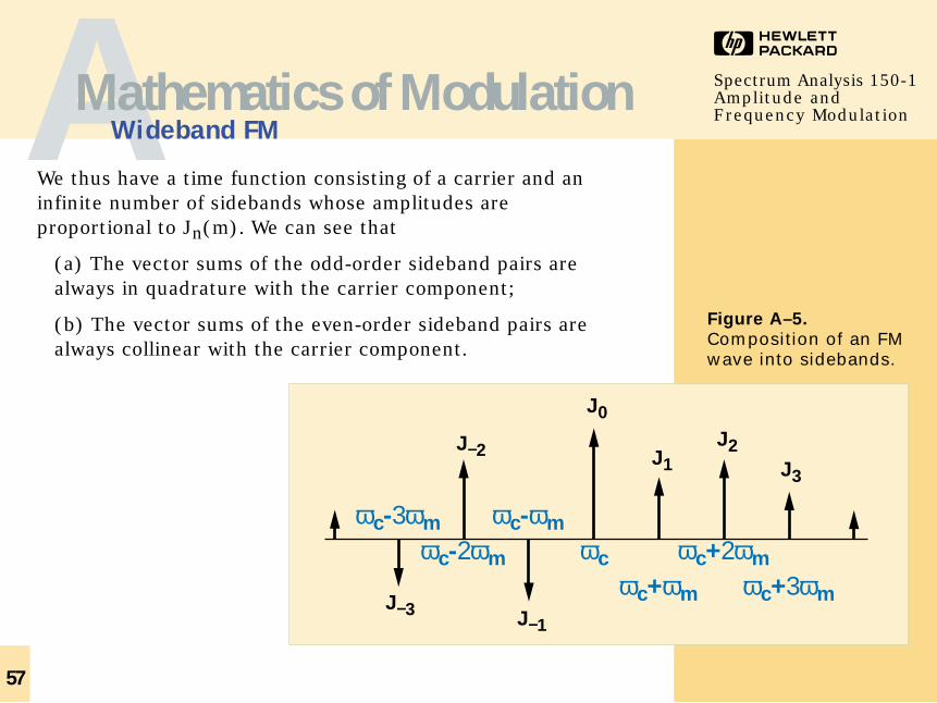
We thus have a time function consisting of a carrier and aninfinite number of sidebands whose amplitudes areproportional to Jn(m). We can see that

(a) The vector sums of the odd-order sideband pairs arealways in quadrature with the carrier component;

(b) The vector sums of the even-order sideband pairs arealways collinear with the carrier component.

AMathematics of ModulationWideband FM

J0

J1

J–1

J2J–2

J3

J–3

ωc+ωm

ωc-ωm

ωc+2ωmωc-2ωm

ωc+3ωm

ωc-3ωm

ωc

Figure A–5.

Composition of an FMwave into sidebands.

Locus of R

ω m t⋅ = π

J (1)0

J (1)1 J (1)1 J (1)2

J (1)31 Radian

R

58


Phasor Diagrams

J (1)0

J (1)1

J (1)2

J (1)3

mω πt⋅ =2

J (1)0

J (1)1

J (1)2 J (1)3

R

ω πm t⋅ = 3

4

Locus of R

ω m t⋅ = 0

J (1)0

J (1)1J (1)1J (1)2

J (1)3

1 Radian

R

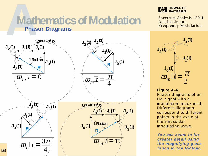
Figure A–6.

Phasor diagrams of anFM signal with amodulation index m=1.Different diagramscorrespond to differentpoints in the cycle ofthe sinusoidalmodulating wave.

You can zoom in forgreater detail usingthe magnifying glassfound in the toolbar.

J (1)0

J (1)1

J (1)2J (1)3

R

ω πm t⋅ = 4

59


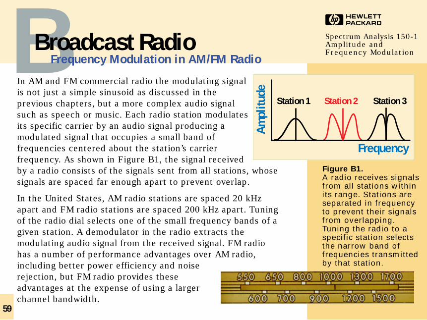
In AM and FM commercial radio the modulating signalis not just a simple sinusoid as discussed in theprevious chapters, but a more complex audio signalsuch as speech or music. Each radio station modulatesits specific carrier by an audio signal producing amodulated signal that occupies a small band offrequencies centered about the station’s carrierfrequency. As shown in Figure B1, the signal receivedby a radio consists of the signals sent from all stations, whosesignals are spaced far enough apart to prevent overlap.

In the United States, AM radio stations are spaced 20 kHzapart and FM radio stations are spaced 200 kHz apart. Tuningof the radio dial selects one of the small frequency bands of agiven station. A demodulator in the radio extracts themodulating audio signal from the received signal. FM radiohas a number of performance advantages over AM radio,including better power efficiency and noiserejection, but FM radio provides theseadvantages at the expense of using a largerchannel bandwidth.

BBroadcast RadioFrequency Modulation in AM/FM Radio


Am

plitu

de

Frequency

Station 1 Station 3Station 2

Figure B1.A radio receives signalsfrom all stations withinits range. Stations areseparated in frequencyto prevent their signalsfrom overlapping.Tuning the radio to aspecific station selectsthe narrow band offrequencies transmittedby that station.

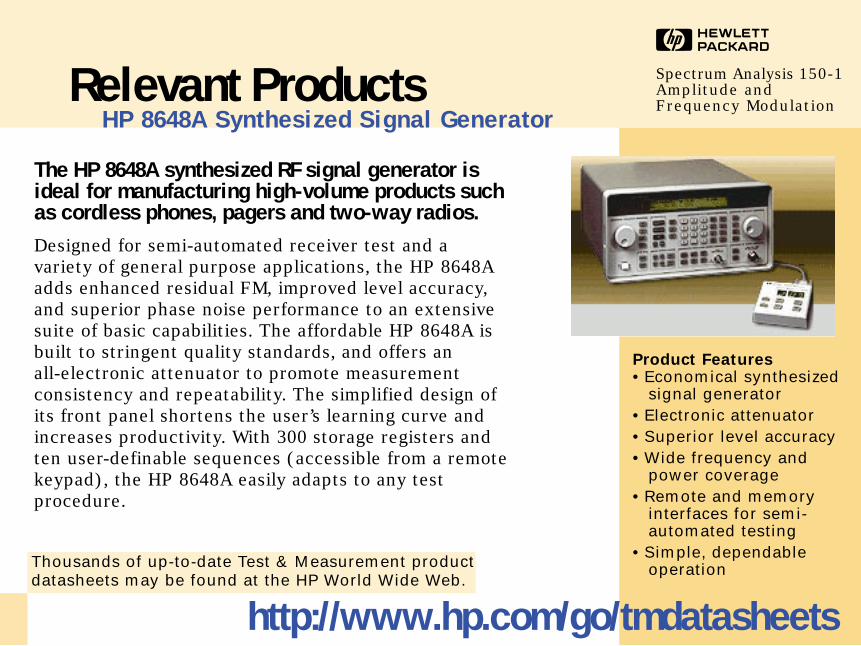
The HP 8648A synthesized RF signal generator isideal for manufacturing high-volume products suchas cordless phones, pagers and two-way radios. Designed for semi-automated receiver test and avariety of general purpose applications, the HP 8648Aadds enhanced residual FM, improved level accuracy,and superior phase noise performance to an extensivesuite of basic capabilities. The affordable HP 8648A isbuilt to stringent quality standards, and offers an all-electronic attenuator to promote measurementconsistency and repeatability. The simplified design ofits front panel shortens the user’s learning curve andincreases productivity. With 300 storage registers andten user-definable sequences (accessible from a remotekeypad), the HP 8648A easily adapts to any testprocedure.


Relevant ProductsHP 8648A Synthesized Signal Generator

Product Features• Economical synthesized

signal generator• Electronic attenuator• Superior level accuracy• Wide frequency and

power coverage• Remote and memory

interfaces for semi-automated testing

• Simple, dependableoperation

http://www.hp.com/go/tmdatasheets

Thousands of up-to-date Test & Measurement productdatasheets may be found at the HP World Wide Web.


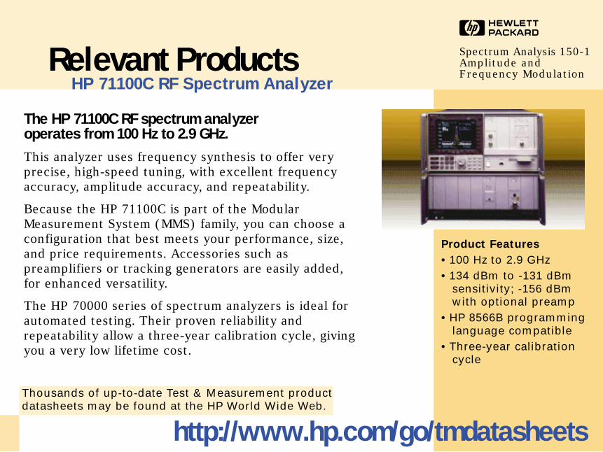
The HP 71100C RF spectrum analyzeroperates from 100 Hz to 2.9 GHz.This analyzer uses frequency synthesis to offer veryprecise, high-speed tuning, with excellent frequencyaccuracy, amplitude accuracy, and repeatability.

Because the HP 71100C is part of the ModularMeasurement System (MMS) family, you can choose aconfiguration that best meets your performance, size,and price requirements. Accessories such aspreamplifiers or tracking generators are easily added,for enhanced versatility.

The HP 70000 series of spectrum analyzers is ideal forautomated testing. Their proven reliability andrepeatability allow a three-year calibration cycle, givingyou a very low lifetime cost.


Relevant ProductsHP 71100C RF Spectrum Analyzer

Product Features

• 100 Hz to 2.9 GHz• 134 dBm to -131 dBm

sensitivity; -156 dBm with optional preamp

• HP 8566B programminglanguage compatible

• Three-year calibrationcycle




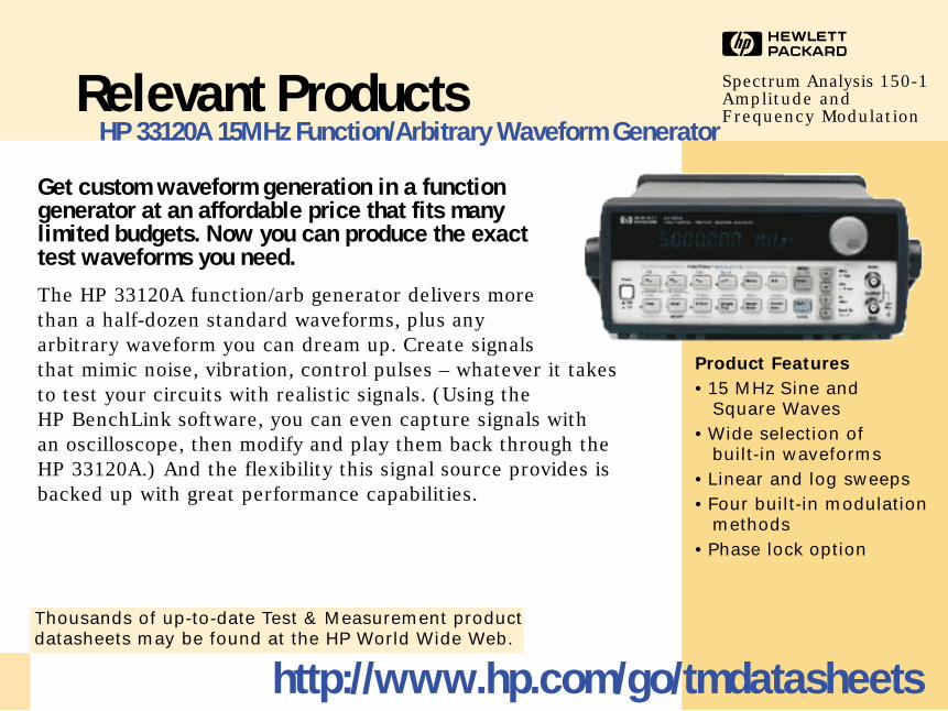
Get custom waveform generation in a functiongenerator at an affordable price that fits manylimited budgets. Now you can produce the exacttest waveforms you need.

The HP 33120A function/arb generator delivers morethan a half-dozen standard waveforms, plus anyarbitrary waveform you can dream up. Create signalsthat mimic noise, vibration, control pulses – whatever it takesto test your circuits with realistic signals. (Using the HP BenchLink software, you can even capture signals with an oscilloscope, then modify and play them back through the HP 33120A.) And the flexibility this signal source provides isbacked up with great performance capabilities.


Relevant ProductsHP 33120A 15MHz Function/Arbitrary Waveform Generator

Product Features

• 15 MHz Sine and Square Waves

• Wide selection of built-in waveforms

• Linear and log sweeps • Four built-in modulation

methods • Phase lock option





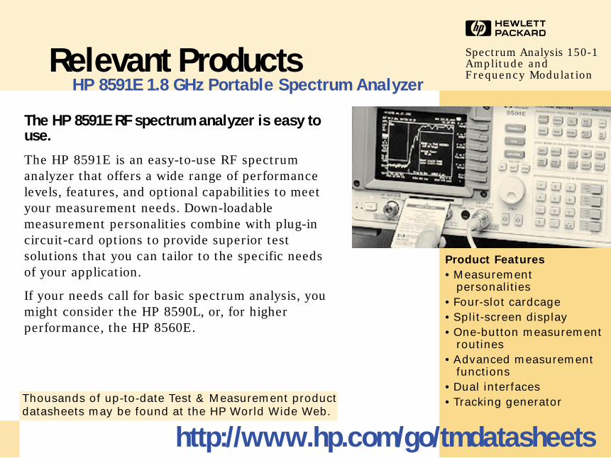
The HP 8591E RF spectrum analyzer is easy touse.

The HP 8591E is an easy-to-use RF spectrumanalyzer that offers a wide range of performancelevels, features, and optional capabilities to meetyour measurement needs. Down-loadablemeasurement personalities combine with plug-incircuit-card options to provide superior testsolutions that you can tailor to the specific needsof your application.

If your needs call for basic spectrum analysis, youmight consider the HP 8590L, or, for higherperformance, the HP 8560E.

Relevant ProductsHP 8591E 1.8 GHz Portable Spectrum Analyzer

Product Features

• Measurementpersonalities

• Four-slot cardcage• Split-screen display• One-button measurement

routines• Advanced measurement

functions• Dual interfaces• Tracking generator





HP offers an extensive curriculum of education servicesat locations worldwide. To help design engineers learnhow to best use their tools, we provide training coursestaught by experts. The HP training program focuses onhow to make accurate measurements using HPinstruments and systems, including spectrum andnetwork analyzers, power meters, vector signalanalyzers, and phase noise systems.

HP education classes are scheduledregularly. The curriculum can be tailored to a company’s special needs, and training sessions can be conducted at its site.

Visit HP’s World Wide Website for the completeand continuously updated list of Test &Measurement class schedules and locationsaround the world. You can register directly online!Click on the URL below or type the address inyour browser.

http://www.hp.com/go/tmeducation

RF and microwave education and trainingRelevant Services

http://www.hp.com/go/tmeducation


Worldwide ContactsHewlett-Packard Test & Measurement Offices

Asia-Pacific

Hewlett-Packard Asia Pacific Ltd.Hewlett-Packard Hong Kong Ltd.17-21/F Shell Tower,Times Square1 Matheson Street, Causeway BayHong Kong85 2 599 7777

For Japan: 0120-421-345

Australia/New Zealand

Hewlett-Packard Australia Ltd.31-41 Joseph StreetBlackburn, Victoria 3130Australia1 800 627 485

Canada

Hewlett-Packard Ltd.5150 Spectrum WayMississauga, Ontario L4W 5G1905-206-4725

Europe/Middle East/Africa

Hewlett-Packard S.A.150, Route du Nant-d’Avril1217 Meyrin 1Geneva, Switzerland

For Europe:41 22 780 81 11

For Middle East/Africa: 41 22 780 41 11

Latin America

Latin American RegionHeadquartersHewlett-Packard CompanyWaterford Building, Suite 9505200 Blue LagoonMiami, FL 33126305-267-4245

United States of America

Hewlett-Packard Company800-452-4844

http://www.hp.com/go/tmdir

Visit HP’s World Wide Website for the complete and up to date listing of Test & Measurement sales officesaddresses and call centers phone numbers worldwide.

http://www.hp.com/go/tmdir


Copyrights and CreditsAuthors, contributors and producers

© Copyright Hewlett-Packard Company 1989, 1996 All Rights Reserved.Adaptation, reproduction, translation, extraction, dissemination ordisassembly without prior written permission is prohibited except asallowed under the copyright laws. Spectrum Analysis Amplitude and

Frequency Modulation is electronically published as part of the HP Test & Measurement Digital Application Note Library for the WorldWide Web, April 1996. Original printed publication Number 5954-9130.

Authors & Contributors

Blake Peterson – 1989 revisionand update; original applicationnote by HP technical staff, 1971.Lee Smith – 1996 revised &updated content, technicalillustrations, mathematicalprogramming, and animations.Jeff Gruszynski – expert domainconsultant, content perspectives.Walt Patstone – technicalcontent review & proof-reading.

Graphic & Interaction Design

Kathy Cunningham – Quarkguru and page layout design.

Christina Bangle – free-styleillustration and graphic reviews.Ev Shafrir – original concept,art direction, interaction design,digital publishing & production,content supervision, overalldirection, & project management.

Business Manager

Nyna Casey – funding, support,excitement, and enthusiasticencouragement of innovation ininteractive publishing.

Amplitude Frequency Modulation - HP Memory Projecthpmemoryproject.org/an/pdf/an_150-1.pdfFrequency...

Documents

Transcript of Amplitude Frequency Modulation - HP Memory Projecthpmemoryproject.org/an/pdf/an_150-1.pdfFrequency...