
AM 205: lecture 16iacs-courses.seas.harvard.edu/courses/am205/fall14/slides/am205... ·...
50
AM 205: lecture 16 I Last time: hyperbolic PDEs I Today: parabolic and elliptic PDEs, introduction to optimization
Transcript of AM 205: lecture 16iacs-courses.seas.harvard.edu/courses/am205/fall14/slides/am205... ·...
AM 205: lecture 16
I Last time: hyperbolic PDEs
I Today: parabolic and elliptic PDEs, introduction tooptimization
The θ-Method: Accuracy
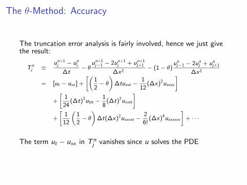
The truncation error analysis is fairly involved, hence we just givethe result:
T nj ≡
un+1j − un
j
∆t− θ
un+1j−1 − 2un+1
j + un+1j+1
∆x2− (1 − θ)
unj−1 − 2un
j + unj+1
∆x2
= [ut − uxx ] +
[(1
2− θ
)∆tuxxt −
1
12(∆x)2uxxxx
]+
[1
24(∆t)2uttt −
1
8(∆t)2uxxtt
]+
[1
12
(1
2− θ
)∆t(∆x)2uxxxxt −
2
6!(∆x)4uxxxxxx
]+ · · ·
The term ut − uxx in T nj vanishes since u solves the PDE
The θ-Method: Accuracy
Key point: This is a first order method, unless θ = 1/2, in whichcase we get a second order method!
θ-method gives us consistency (at least first order) and stability(assuming ∆t is chosen appropriately when θ ∈ [0, 1/2))
Hence, from Lax Equivalence Theorem, the method is convergent
The Heat Equation
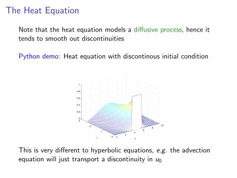
Note that the heat equation models a diffusive process, hence ittends to smooth out discontinuities
Python demo: Heat equation with discontinous initial condition
0
2
4
6
8
10
0
1
2
3
0
0.2
0.4
0.6
0.8
1
xt
This is very different to hyperbolic equations, e.g. the advectionequation will just transport a discontinuity in u0

Elliptic PDEs
Elliptic PDEs
The canonical elliptic PDE is the Poisson equation
In one-dimension, for x ∈ [a, b], this is −u′′(x) = f (x) withboundary conditions at x = a and x = b
We have seen this problem already: Two-point boundary valueproblem!
(Recall that Elliptic PDEs model steady-state behavior, there is notime-derivative)
Elliptic PDEs
In order to make this into a PDE, we need to consider more thanone spatial dimension
Let Ω ⊂ R2 denote our domain, then the Poisson equation for(x , y) ∈ Ω is
uxx + uyy = f (x , y)
This is generally written more succinctly as ∆u = f
We again need to impose boundary conditions (Dirichlet,Neumann, or Robin) on ∂Ω (recall ∂Ω denotes boundary of Ω)
Elliptic PDEs
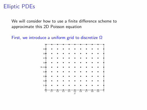
We will consider how to use a finite difference scheme toapproximate this 2D Poisson equation
First, we introduce a uniform grid to discretize Ω
0 0.1 0.2 0.3 0.4 0.5 0.6 0.7 0.8 0.9 10
0.1
0.2
0.3
0.4
0.5
0.6
0.7
0.8
0.9
1
x
y
Elliptic PDEs
Let h = ∆x = ∆y denote the grid spacing
Then,
I xi = ih, i = 0, 1, 2 . . . , nx − 1,
I yj = jh, j = 0, 1, 2, . . . , ny − 1,
I Ui ,j ≈ u(xi , yj)
Then, we need to be able to approximate uxx and uyy on this grid
Natural idea: Use central difference approximation!
Elliptic PDEs
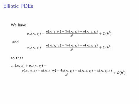
We have
uxx(xi , yj) =u(xi−1, yj) − 2u(xi , yj) + u(xi+1, yj)
h2+ O(h2),
anduyy (xi , yj) =
u(xi , yj−1) − 2u(xi , yj) + u(xi , yj+1)
h2+ O(h2),
so that
uxx(xi , yj) + uyy (xi , yj) =
u(xi , yj−1) + u(xi−1, yj) − 4u(xi , yj) + u(xi+1, yj) + u(xi , yj+1)
h2+ O(h2)
Elliptic PDEs
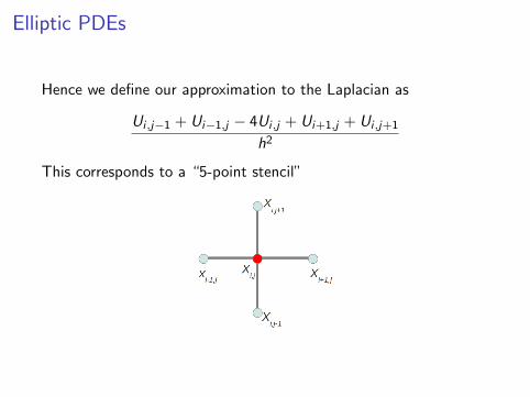
Hence we define our approximation to the Laplacian as
Ui ,j−1 + Ui−1,j − 4Ui ,j + Ui+1,j + Ui ,j+1
h2
This corresponds to a “5-point stencil”
Elliptic PDEs
As usual, we represent the numerical solution as a vector U ∈ Rnxny
We want to construct a differentiation matrix D2 ∈ Rnxny×nxny
that approximates the Laplacian
Question: How many non-zero diagonals will D2 have?
To construct D2, we need to be able to relate the entries of thevector U to the “2D grid-based values” Ui ,j
Elliptic PDEs
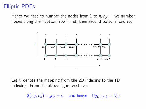
Hence we need to number the nodes from 1 to nxny — we numbernodes along the “bottom row” first, then second bottom row, etc
Let G denote the mapping from the 2D indexing to the 1Dindexing. From the above figure we have:
G(i , j ; nx) = jnx + i , and hence UG(i ,j ;nx ) = Ui ,j
Elliptic PDEs
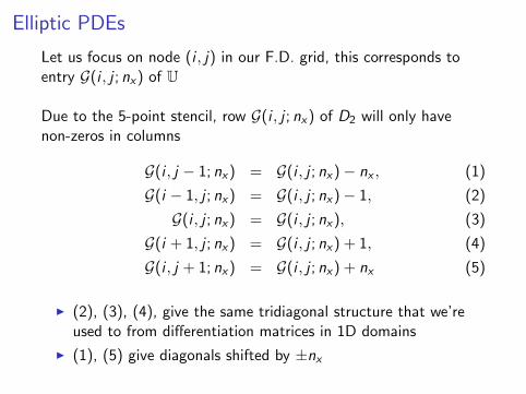
Let us focus on node (i , j) in our F.D. grid, this corresponds toentry G(i , j ; nx) of U
Due to the 5-point stencil, row G(i , j ; nx) of D2 will only havenon-zeros in columns
G(i , j − 1; nx) = G(i , j ; nx)− nx , (1)
G(i − 1, j ; nx) = G(i , j ; nx)− 1, (2)
G(i , j ; nx) = G(i , j ; nx), (3)
G(i + 1, j ; nx) = G(i , j ; nx) + 1, (4)
G(i , j + 1; nx) = G(i , j ; nx) + nx (5)
I (2), (3), (4), give the same tridiagonal structure that we’reused to from differentiation matrices in 1D domains
I (1), (5) give diagonals shifted by ±nx
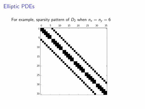
Elliptic PDEs
For example, sparsity pattern of D2 when nx = ny = 6
Elliptic PDEs
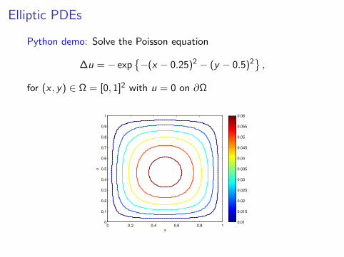
Python demo: Solve the Poisson equation
∆u = − exp−(x − 0.25)2 − (y − 0.5)2
,
for (x , y) ∈ Ω = [0, 1]2 with u = 0 on ∂Ω
x
y
0 0.2 0.4 0.6 0.8 10
0.1
0.2
0.3
0.4
0.5
0.6
0.7
0.8
0.9
1
0.01
0.015
0.02
0.025
0.03
0.035
0.04
0.045
0.05
0.055
0.06
Nonlinear Equations and Optimization
Motivation: Nonlinear Equations
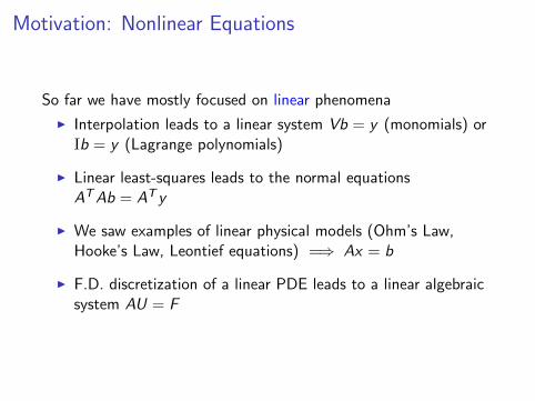
So far we have mostly focused on linear phenomena
I Interpolation leads to a linear system Vb = y (monomials) orIb = y (Lagrange polynomials)
I Linear least-squares leads to the normal equationsATAb = AT y
I We saw examples of linear physical models (Ohm’s Law,Hooke’s Law, Leontief equations) =⇒ Ax = b
I F.D. discretization of a linear PDE leads to a linear algebraicsystem AU = F
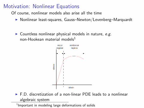
Motivation: Nonlinear EquationsOf course, nonlinear models also arise all the time
I Nonlinear least-squares, Gauss–Newton/Levenberg–Marquardt
I Countless nonlinear physical models in nature, e.g.non-Hookean material models1
I F.D. discretization of a non-linear PDE leads to a nonlinearalgebraic system
1Important in modeling large deformations of solids
Motivation: Nonlinear Equations
Another example is computation of Gauss quadraturepoints/weights
We know this is possible via roots of Legendre polynomials
But we could also try to solve the nonlinear system of equationsfor (x1,w1), (x2,w2), . . . , (xn,wn)
Motivation: Nonlinear Equations
e.g. for n = 2, we need to find points/weights such that allpolynomials of degree 3 are integrated exactly, hence
w1 + w2 =
∫ 1
−11dx = 2
w1x1 + w2x2 =
∫ 1
−1xdx = 0
w1x21 + w2x
22 =
∫ 1
−1x2dx = 2/3
w1x31 + w2x
32 =
∫ 1
−1x3dx = 0
Motivation: Nonlinear Equations
We usually write a nonlinear system of equations as
F (x) = 0,
where F : Rn → Rm
We implicity absorb the “right-hand side” into F and seek a rootof F
In this Unit we focus on the case m = n, m > n gives nonlinearleast-squares
Motivation: Nonlinear Equations
We are very familiar with scalar (m = 1) nonlinear equations
Simplest case is a quadratic equation
ax2 + bx + c = 0
We can write down a closed form solution, the quadratic formula
x =−b ±
√b2 − 4ac
2a
Motivation: Nonlinear Equations
In fact, there are also closed-form solutions for arbitrary cubic andquartic polynomials, due to Ferrari and Cardano (∼ 1540)
Important mathematical result is that there is no general formulafor solving fifth or higher order polynomial equations
Hence, even for the simplest possible case (polynomials), the onlyhope is to employ an iterative algorithm
An iterative method should converge in the limit n→∞, andideally yields an accurate approximation after few iterations
Motivation: Nonlinear Equations
There are many well-known iterative methods for nonlinearequations
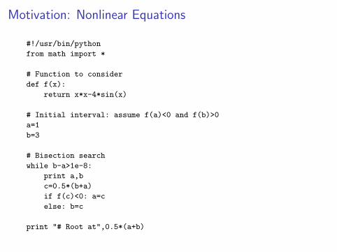
Probably the simplest is the bisection method for a scalar equationf (x) = 0, where f ∈ C [a, b]
Look for a root in the interval [a, b] by bisecting based on sign of f
Motivation: Nonlinear Equations
#!/usr/bin/python
from math import *
# Function to consider
def f(x):
return x*x-4*sin(x)
# Initial interval: assume f(a)<0 and f(b)>0
a=1
b=3
# Bisection search
while b-a>1e-8:
print a,b
c=0.5*(b+a)
if f(c)<0: a=c
else: b=c
print "# Root at",0.5*(a+b)
Motivation: Nonlinear Equations
1 1.5 2 2.5 3−4
−2
0
2
4
6
8
10
1.932 1.933 1.934 1.935
−0.01
−0.005
0
0.005
0.01
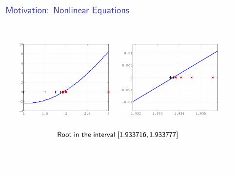
Root in the interval [1.933716, 1.933777]
Motivation: Nonlinear Equations
Bisection is a robust root-finding method in 1D, but it does notgeneralize easily to Rn for n > 1
Also, bisection is a crude method in the sense that it makes no useof magnitude of f , only sign(f )
We will look at mathematical basis of alternative methods whichgeneralize to Rn:
I Fixed-point iteration
I Newton’s method

Optimization
Motivation: Optimization
Another major topic in Scientific Computing is optimization
Very important in science, engineering, industry, finance,economics, logistics,...
Many engineering challenges can be formulated as optimizationproblems, e.g.:
I Design car body that maximizes downforce2
I Design a bridge with minimum weight
2A major goal in racing car design
Motivation: Optimization
Of course, in practice, it is more realistic to consider optimizationproblems with constraints, e.g.:
I Design car body that maximizes downforce, subject to aconstraint on drag
I Design a bridge with minimum weight, subject to a constrainton strength
Motivation: Optimization
Also, (constrained and unconstrained) optimization problems arisenaturally in science
Physics:
I many physical systems will naturally occupy a minimumenergy state
I if we can describe the energy of the system mathematically,then we can find minimum energy state via optimization
Motivation: Optimization
Biology:
I recent efforts in Scientific Computing have sought tounderstand biological phenomena quantitively via optimization
I computational optimization of, e.g. fish swimming or insectflight, can reproduce behavior observed in nature
I this jells with the idea that evolution has been “optimizing”organisms for millions of year
Motivation: Optimization
All these problems can be formulated as: Optimize (max. or min.)an objective function over a set of feasible choices, i.e.
Given an objective function f : Rn → R and a set S ⊂ Rn,we seek x∗ ∈ S such that f (x∗) ≤ f (x), ∀x ∈ S
(It suffices to consider only minimization, maximization isequivalent to minimizing −f )
S is the feasible set, usually defined by a set of equations and/orinequalities, which are the constraints
If S = Rn, then the problem is unconstrained
Motivation: Optimization
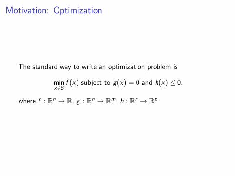
The standard way to write an optimization problem is
minx∈S
f (x) subject to g(x) = 0 and h(x) ≤ 0,
where f : Rn → R, g : Rn → Rm, h : Rn → Rp
Motivation: Optimization
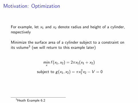
For example, let x1 and x2 denote radius and height of a cylinder,respectively
Minimize the surface area of a cylinder subject to a constraint onits volume3 (we will return to this example later)
minx
f (x1, x2) = 2πx1(x1 + x2)
subject to g(x1, x2) = πx21x2 − V = 0
3Heath Example 6.2
Motivation: Optimization
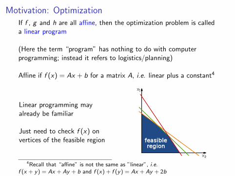
If f , g and h are all affine, then the optimization problem is calleda linear program
(Here the term “program” has nothing to do with computerprogramming; instead it refers to logistics/planning)
Affine if f (x) = Ax + b for a matrix A, i.e. linear plus a constant4
Linear programming mayalready be familiar
Just need to check f (x) onvertices of the feasible region
4Recall that “affine” is not the same as ”linear”, i.e.f (x + y) = Ax + Ay + b and f (x) + f (y) = Ax + Ay + 2b
Motivation: Optimization
If the objective function or any of the constraints are nonlinear thenwe have a nonlinear optimization problem or nonlinear program
We will consider several different approaches to nonlinearoptimization in this Unit
Optimization routines typically use local information about afunction to iteratively approach a local minimum
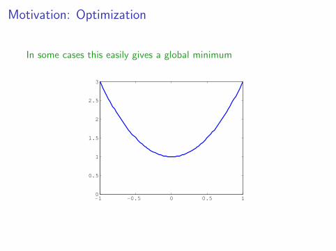
Motivation: Optimization
In some cases this easily gives a global minimum
−1 −0.5 0 0.5 10
0.5
1
1.5
2
2.5
3
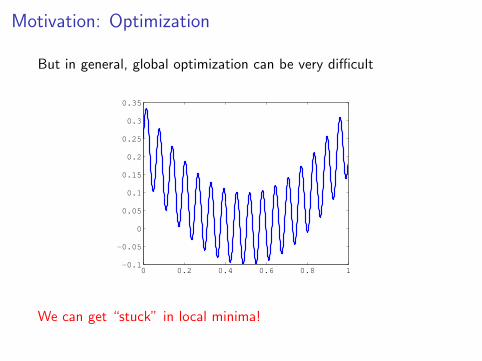
Motivation: Optimization
But in general, global optimization can be very difficult
0 0.2 0.4 0.6 0.8 1−0.1
−0.05
0
0.05
0.1
0.15
0.2
0.25
0.3
0.35
We can get “stuck” in local minima!
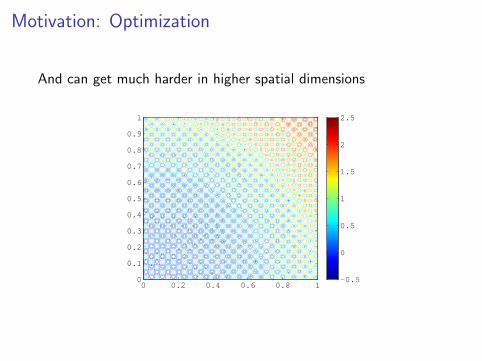
Motivation: Optimization
And can get much harder in higher spatial dimensions
0 0.2 0.4 0.6 0.8 10
0.1
0.2
0.3
0.4
0.5
0.6
0.7
0.8
0.9
1
−0.5
0
0.5
1
1.5
2
2.5
Motivation: Optimization
There are robust methods for finding local minimima, and this iswhat we focus on in AM205
Global optimization is very important in practice, but in generalthere is no way to guarantee that we will find a global minimum
Global optimization basically relies on heuristics:
I try several different starting guesses (“multistart” methods)
I simulated annealing
I genetic methods5
5Simulated annealing and genetic methods are covered in AM207
Root Finding: Scalar Case
Fixed-Point Iteration
Suppose we define an iteration
xk+1 = g(xk) (∗)
e.g. recall Heron’s Method from Assignment 0 for finding√a:
xk+1 =1
2
(xk +
a
xk
)This uses gheron(x) = 1
2 (x + a/x)
Fixed-Point Iteration
Suppose α is such that g(α) = α, then we call α a fixed point of g
For example, we see that√a is a fixed point of gheron since
gheron(√a) =
1
2
(√a + a/
√a)
=√a
A fixed-point iteration terminates once a fixed point is reached,since if g(xk) = xk then we get xk+1 = xk
Also, if xk+1 = g(xk) converges as k →∞, it must converge to afixed point: Let α ≡ limk→∞ xk , then6
α = limk→∞
xk+1 = limk→∞
g(xk) = g
(limk→∞
xk
)= g(α)
6Third equality requires g to be continuous
Fixed-Point Iteration
Hence, for example, we know if Heron’s method converges, it willconverge to
√a
It would be very helpful to know when we can guarantee that afixed-point iteration will converge
Recall that g satisfies a Lipschitz condition in an interval [a, b] if∃L ∈ R>0 such that
|g(x)− g(y)| ≤ L|x − y |, ∀x , y ∈ [a, b]
g is called a contraction if L < 1
Fixed-Point Iteration
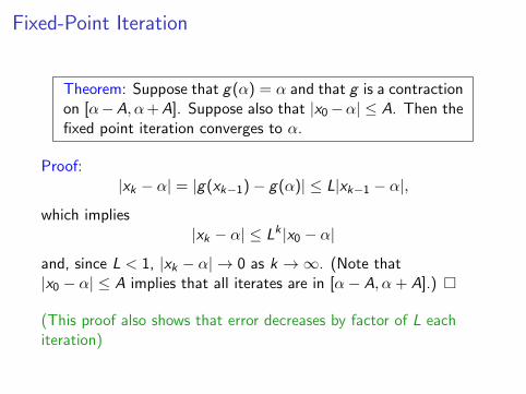
Theorem: Suppose that g(α) = α and that g is a contractionon [α−A, α+A]. Suppose also that |x0−α| ≤ A. Then thefixed point iteration converges to α.
Proof:|xk − α| = |g(xk−1)− g(α)| ≤ L|xk−1 − α|,
which implies|xk − α| ≤ Lk |x0 − α|
and, since L < 1, |xk − α| → 0 as k →∞. (Note that|x0 − α| ≤ A implies that all iterates are in [α− A, α + A].)
(This proof also shows that error decreases by factor of L eachiteration)
Fixed-Point Iteration
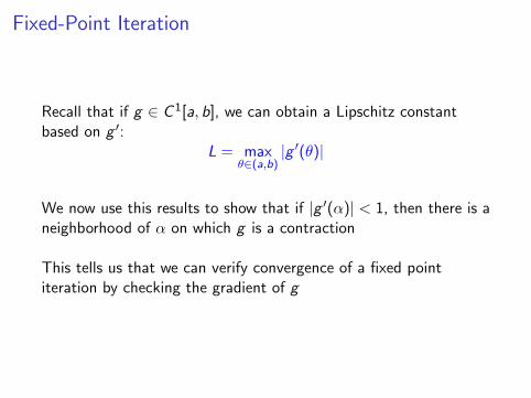
Recall that if g ∈ C 1[a, b], we can obtain a Lipschitz constantbased on g ′:
L = maxθ∈(a,b)
|g ′(θ)|
We now use this results to show that if |g ′(α)| < 1, then there is aneighborhood of α on which g is a contraction
This tells us that we can verify convergence of a fixed pointiteration by checking the gradient of g
Fixed-Point Iteration
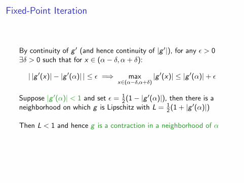
By continuity of g ′ (and hence continuity of |g ′|), for any ε > 0∃δ > 0 such that for x ∈ (α− δ, α + δ):
| |g ′(x)| − |g ′(α)| | ≤ ε =⇒ maxx∈(α−δ,α+δ)
|g ′(x)| ≤ |g ′(α)|+ ε
Suppose |g ′(α)| < 1 and set ε = 12(1− |g ′(α)|), then there is a
neighborhood on which g is Lipschitz with L = 12(1 + |g ′(α)|)
Then L < 1 and hence g is a contraction in a neighborhood of α
Fixed-Point Iteration
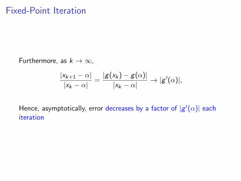
Furthermore, as k →∞,
|xk+1 − α||xk − α|
=|g(xk)− g(α)||xk − α|
→ |g ′(α)|,
Hence, asymptotically, error decreases by a factor of |g ′(α)| eachiteration


![Zajj Daugherty...2018/07/16 · C[[x 1;x 2;:::]] consisting of series where the coe cients on the monomials x 1 1 x 2 2 x ‘ ‘ and x 1 i 1 x 2 i 2 x ‘ i ‘ are the same, for](https://static.fdocument.org/doc/165x107/61289ec787b1fe0e690fc247/zajj-daugherty-20180716-cx-1x-2-consisting-of-series-where-the.jpg)