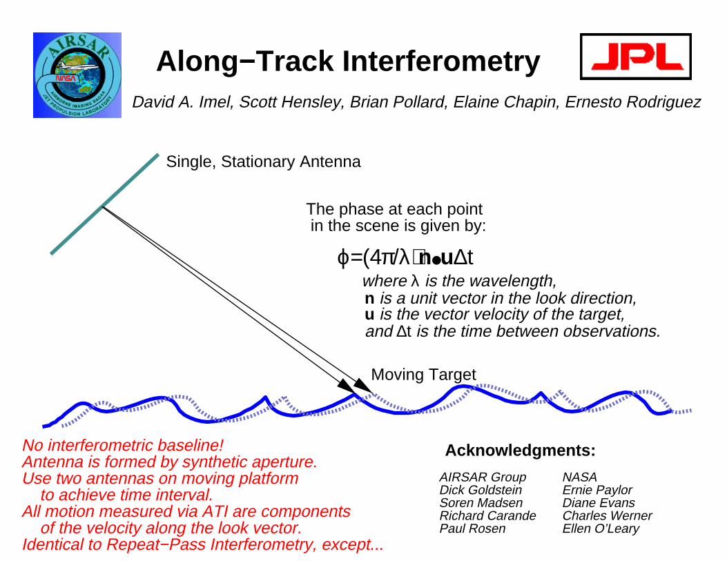
Along−Track Interferometry

Single, Stationary Antenna

Moving Target

No interferometric baseline!Antenna is formed by synthetic aperture.Use two antennas on moving platform to achieve time interval.All motion measured via ATI are components of the velocity along the look vector.Identical to Repeat−Pass Interferometry, except...

ϕ=(4π/λ)n●u∆t where λ is the wavelength, n is a unit vector in the look direction, u is the vector velocity of the target, and ∆t is the time between observations.

The phase at each point in the scene is given by:

Acknowledgments:

David A. Imel, Scott Hensley, Brian Pollard, Elaine Chapin, Ernesto Rodriguez

AIRSAR GroupDick GoldsteinSoren MadsenRichard CarandePaul Rosen

NASA Ernie PaylorDiane EvansCharles WernerEllen O’Leary

Why ATI?

Provides a direct measurement of velocity (vs. altimetry).

Highlights ocean boundaries (wave velocity vs. height).

Direct measurement of ocean coherence time.

Better wave spectra than conventional SAR.

Detection of moving targets: vehicles, ships, wakes.

Mapping of surfactants, upwelling, pollution, surf−zones.

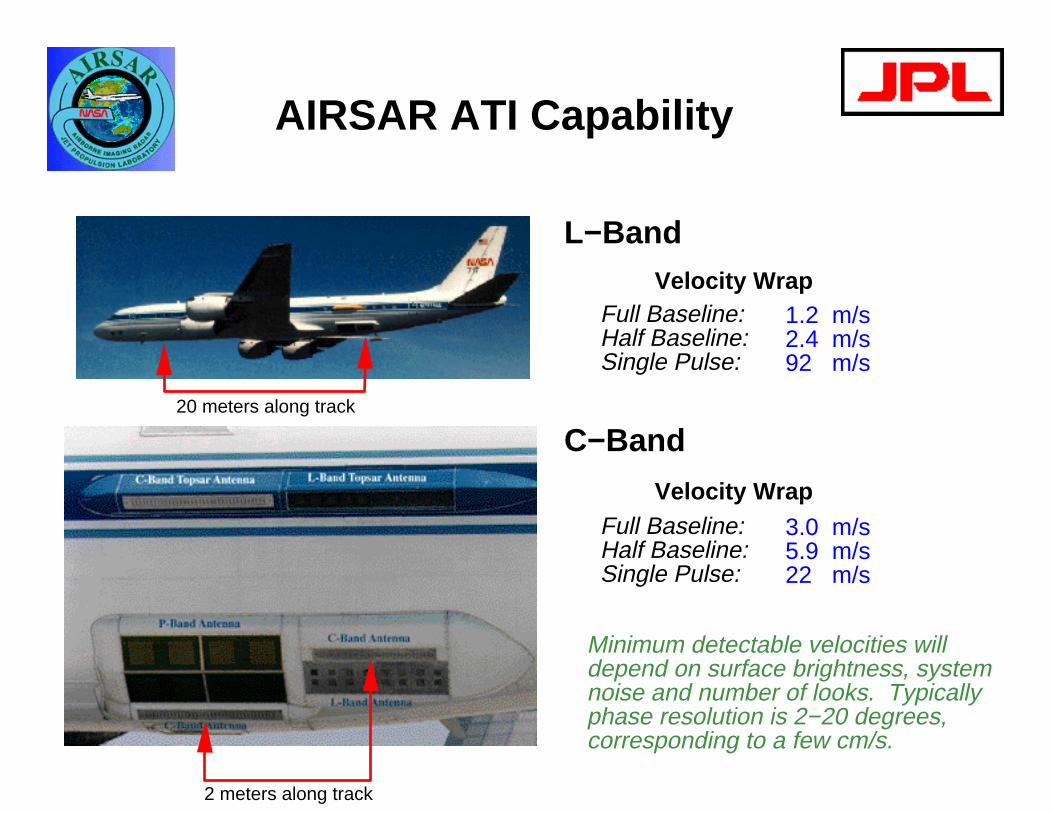
AIRSAR ATI Capability

20 meters along track

2 meters along track

Minimum detectable velocities willdepend on surface brightness, systemnoise and number of looks. Typicallyphase resolution is 2−20 degrees,corresponding to a few cm/s.

C−Band

Velocity WrapFull Baseline:Half Baseline:Single Pulse:

3.0 m/s5.9 m/s22 m/s

L−BandVelocity Wrap

Full Baseline:Half Baseline:Single Pulse:

1.2 m/s2.4 m/s92 m/s

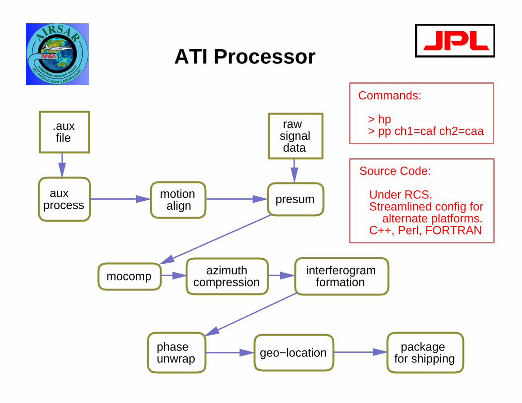
ATI Processor

rawsignal data

.aux file

auxprocess

motion align presum

phaseunwrap geo−location package

for shipping

mocomp azimuthcompression

interferogram formation

Commands:

> hp > pp ch1=caf ch2=caa

Source Code:

Under RCS. Streamlined config for alternate platforms. C++, Perl, FORTRAN

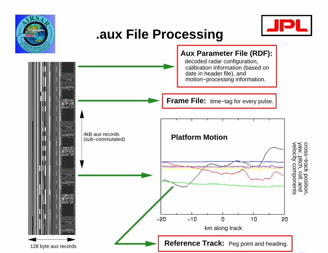
km along track

cross−track position,

yaw, pitch, roll, and

velocity components

.aux File Processing

Platform Motion

128 byte aux records

Aux Parameter File (RDF): decoded radar configuration, calibration information (based on date in header file), and motion−processing information.

Reference Track: Peg point and heading.

4kB aux records(sub−commutated)

Frame File: time−tag for every pulse.

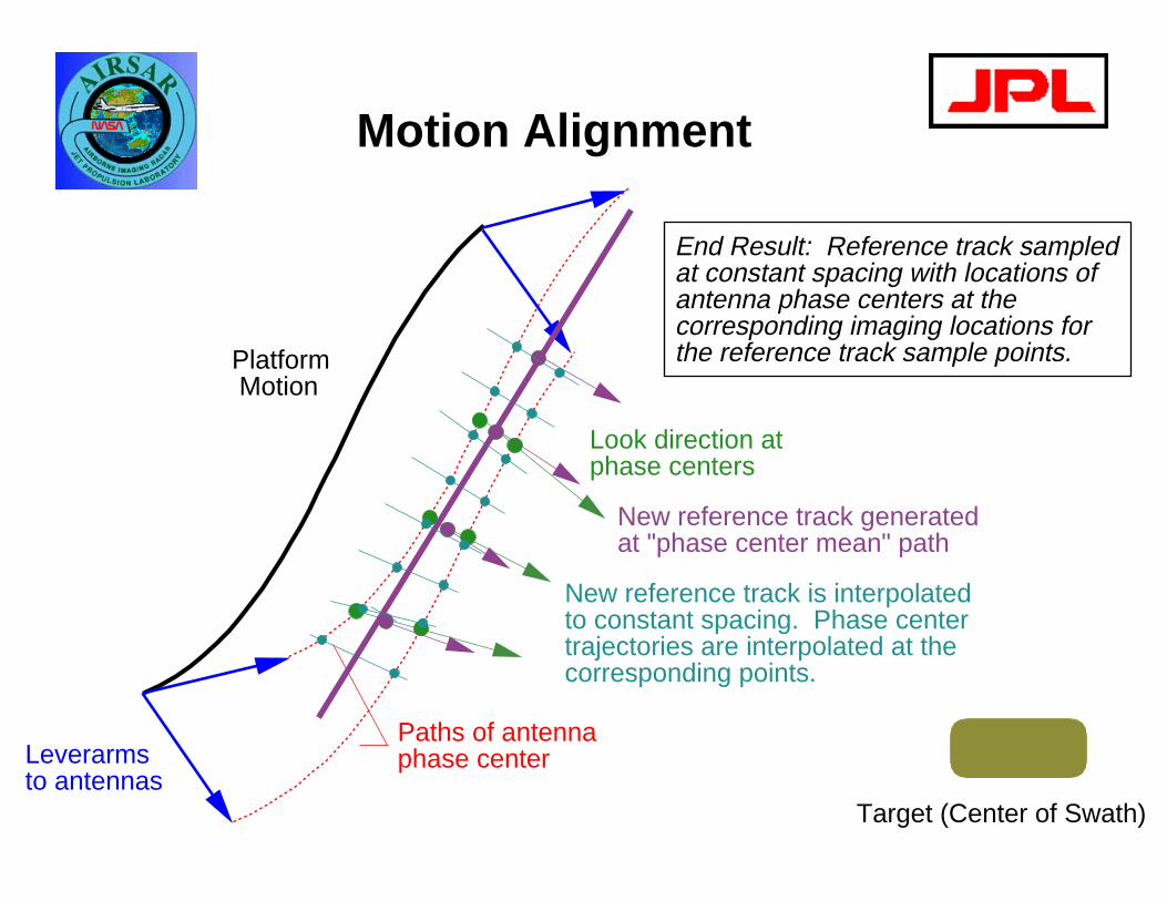
Motion Alignment

Leverarmsto antennas

Paths of antennaphase center

Platform Motion

Target (Center of Swath)

Look direction atphase centers

New reference track generatedat "phase center mean" path

New reference track is interpolatedto constant spacing. Phase centertrajectories are interpolated at thecorresponding points.

End Result: Reference track sampledat constant spacing with locations ofantenna phase centers at the corresponding imaging locations forthe reference track sample points.

AIRSAR Signal Data"Point Target Simulator Simulator"

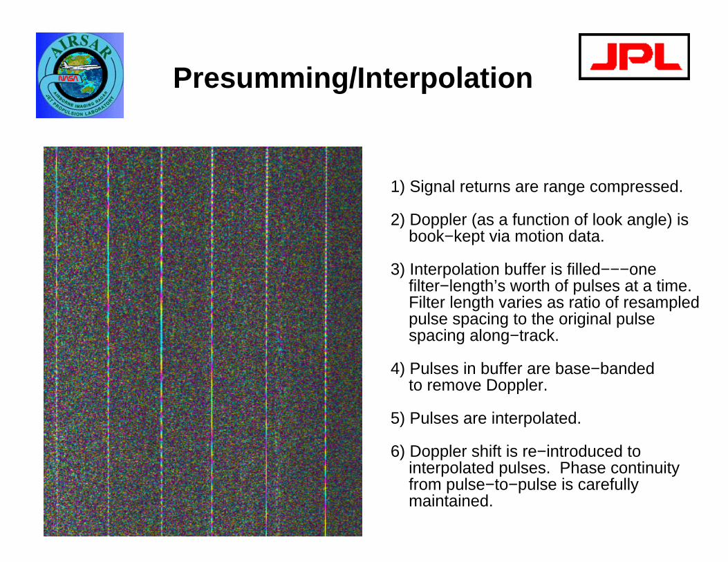
Presumming/Interpolation

1) Signal returns are range compressed.

2) Doppler (as a function of look angle) is book−kept via motion data.

3) Interpolation buffer is filled−−−one filter−length’s worth of pulses at a time. Filter length varies as ratio of resampled pulse spacing to the original pulse spacing along−track.

4) Pulses in buffer are base−banded to remove Doppler.

5) Pulses are interpolated.

6) Doppler shift is re−introduced to interpolated pulses. Phase continuity from pulse−to−pulse is carefully maintained.

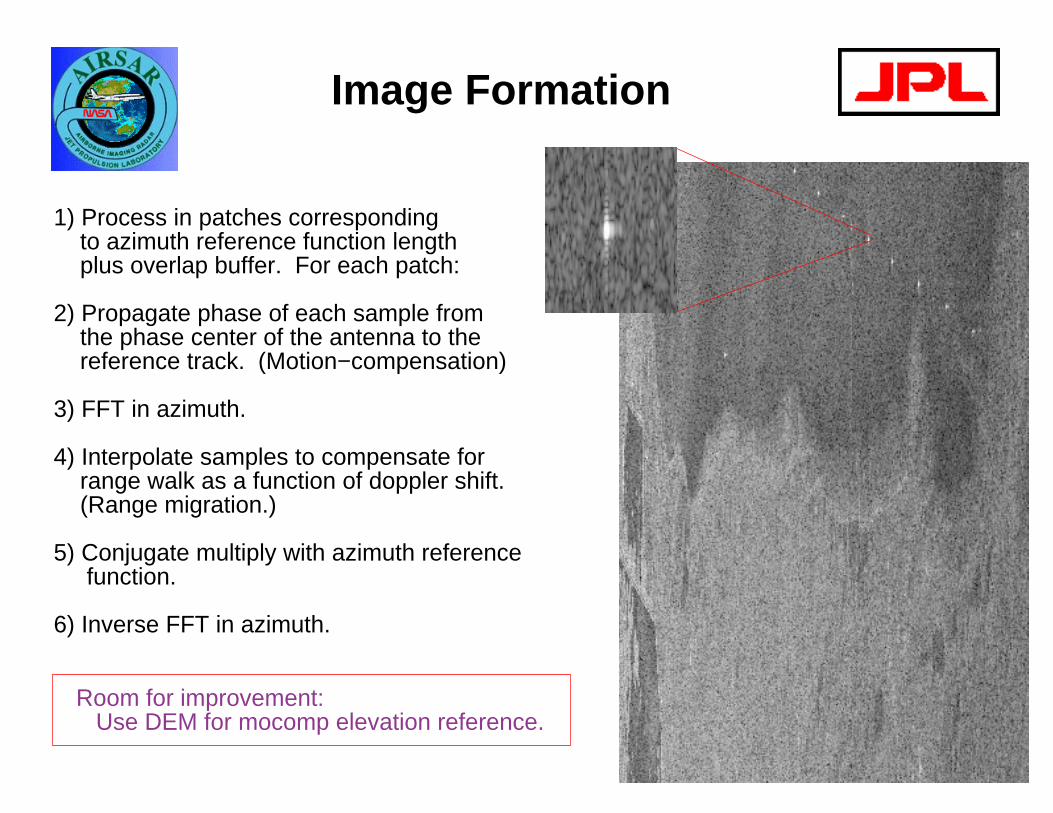
Image Formation

1) Process in patches corresponding to azimuth reference function length plus overlap buffer. For each patch:

2) Propagate phase of each sample from the phase center of the antenna to the reference track. (Motion−compensation)

3) FFT in azimuth.

4) Interpolate samples to compensate for range walk as a function of doppler shift. (Range migration.)

5) Conjugate multiply with azimuth reference function.

6) Inverse FFT in azimuth.

Room for improvement: Use DEM for mocomp elevation reference.

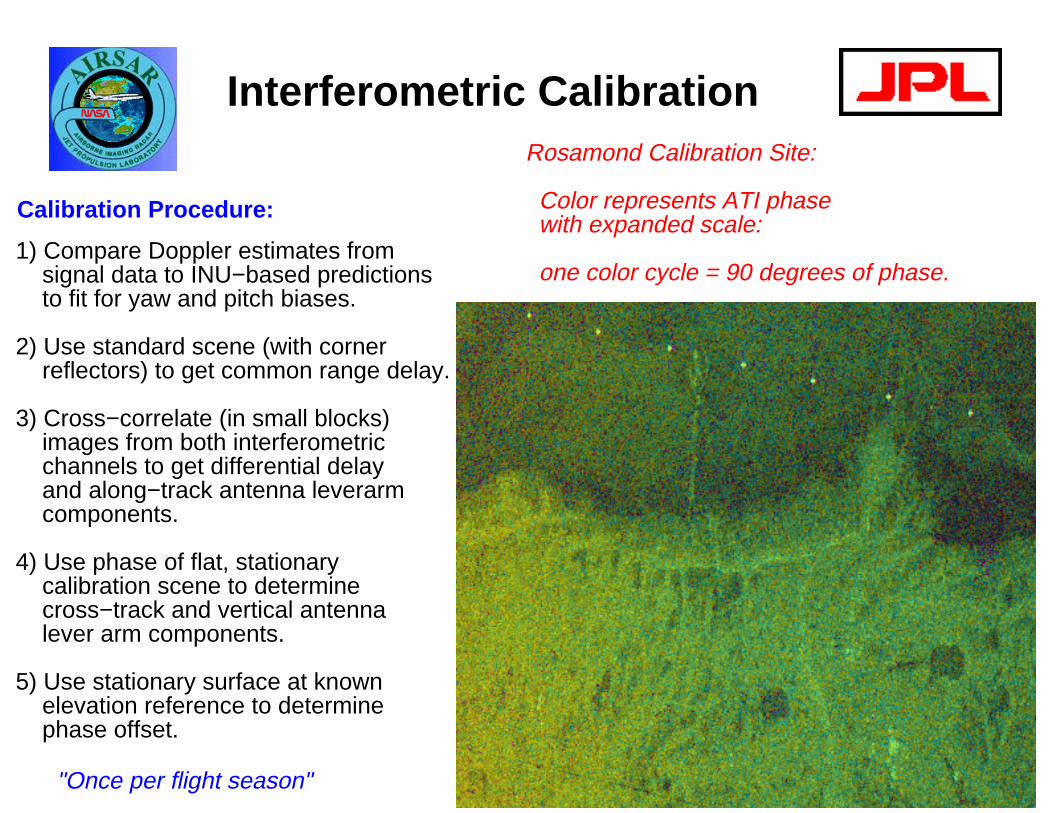
Interferometric Calibration

1) Compare Doppler estimates from signal data to INU−based predictions to fit for yaw and pitch biases.

2) Use standard scene (with corner reflectors) to get common range delay.

3) Cross−correlate (in small blocks) images from both interferometric channels to get differential delay and along−track antenna leverarm components.

4) Use phase of flat, stationary calibration scene to determine cross−track and vertical antenna lever arm components.

5) Use stationary surface at known elevation reference to determine phase offset.

Rosamond Calibration Site:

Color represents ATI phase with expanded scale:

one color cycle = 90 degrees of phase.

Calibration Procedure:

"Once per flight season"

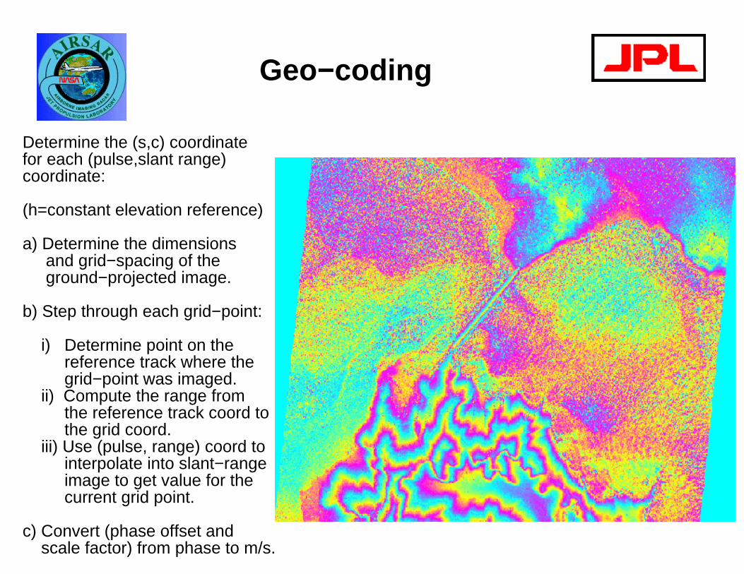
Geo−coding

Determine the (s,c) coordinate for each (pulse,slant range)coordinate: (h=constant elevation reference)

a) Determine the dimensions and grid−spacing of the ground−projected image.

b) Step through each grid−point: i) Determine point on the reference track where the grid−point was imaged. ii) Compute the range from the reference track coord to the grid coord. iii) Use (pulse, range) coord to interpolate into slant−range image to get value for the current grid point.

c) Convert (phase offset and scale factor) from phase to m/s.

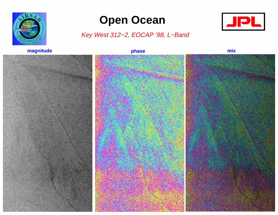
Open Ocean

magnitude phase mix

Key West 312−2, EOCAP ’98, L−Band

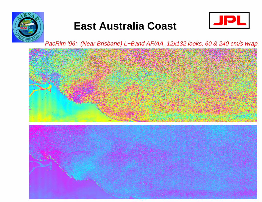
East Australia Coast

PacRim ’96: (Near Brisbane) L−Band AF/AA, 12x132 looks, 60 & 240 cm/s wrap

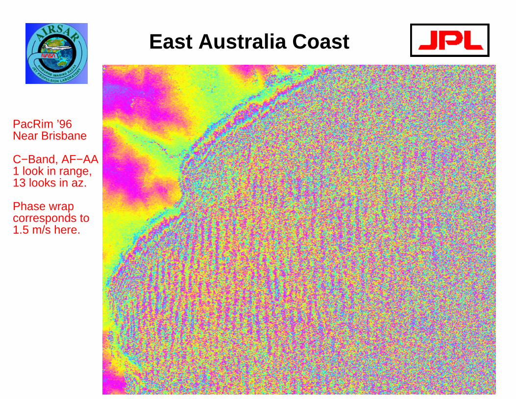
East Australia Coast

PacRim ’96Near Brisbane

C−Band, AF−AA1 look in range,13 looks in az.

Phase wrap corresponds to1.5 m/s here.

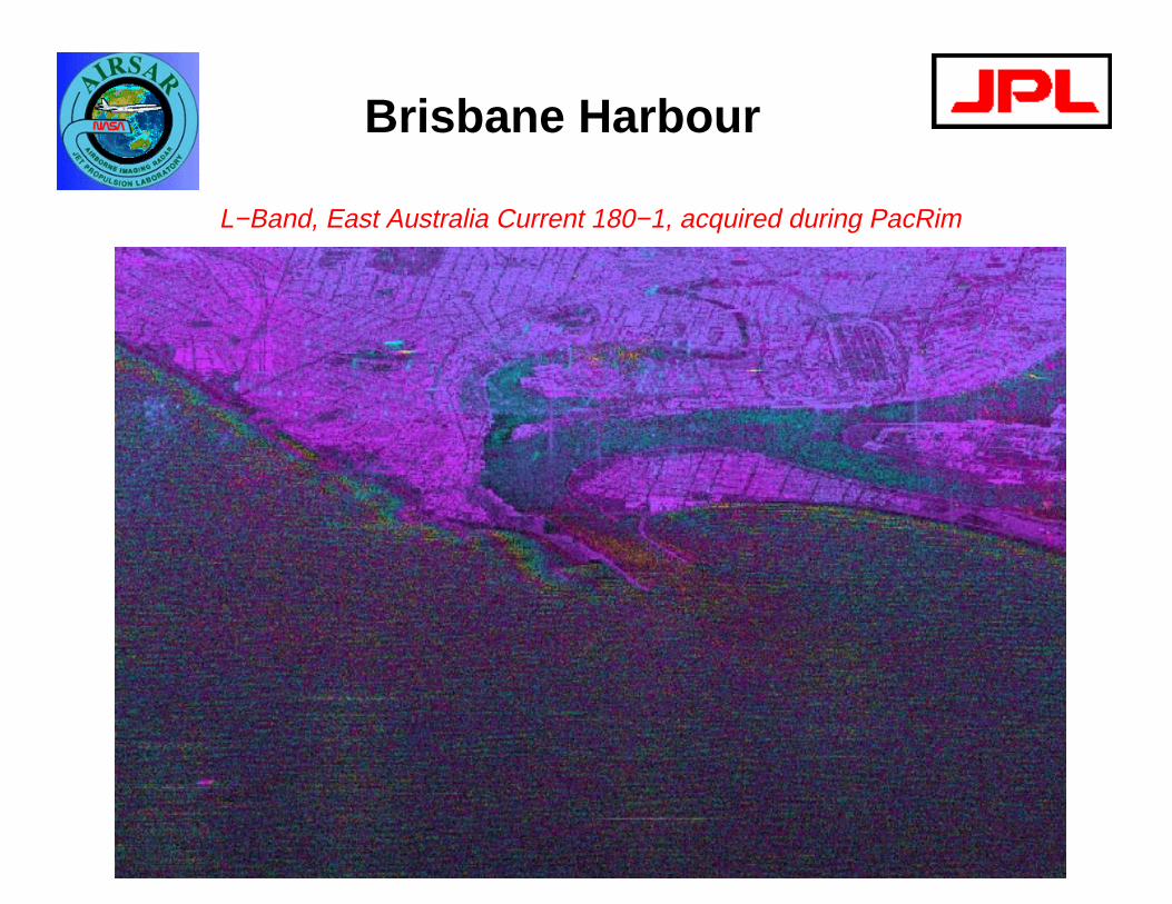
Brisbane Harbour

L−Band, East Australia Current 180−1, acquired during PacRim

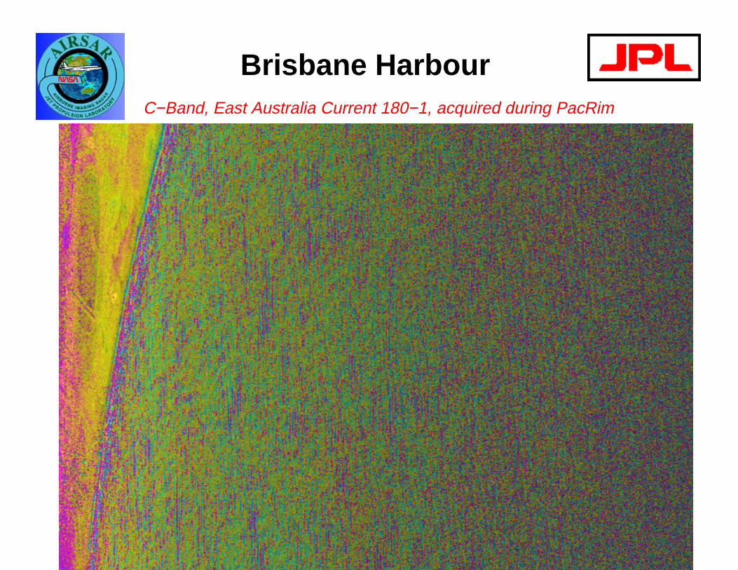
Brisbane HarbourC−Band, East Australia Current 180−1, acquired during PacRim

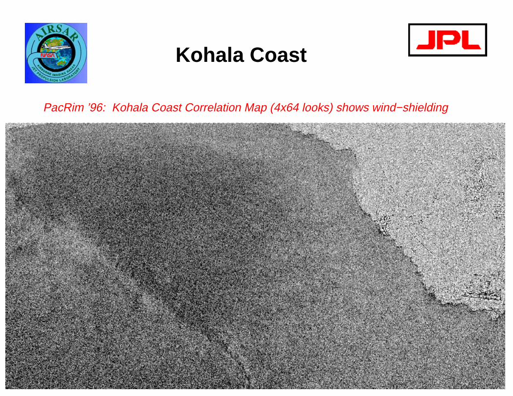
Kohala Coast

PacRim ’96: Kohala Coast Correlation Map (4x64 looks) shows wind−shielding

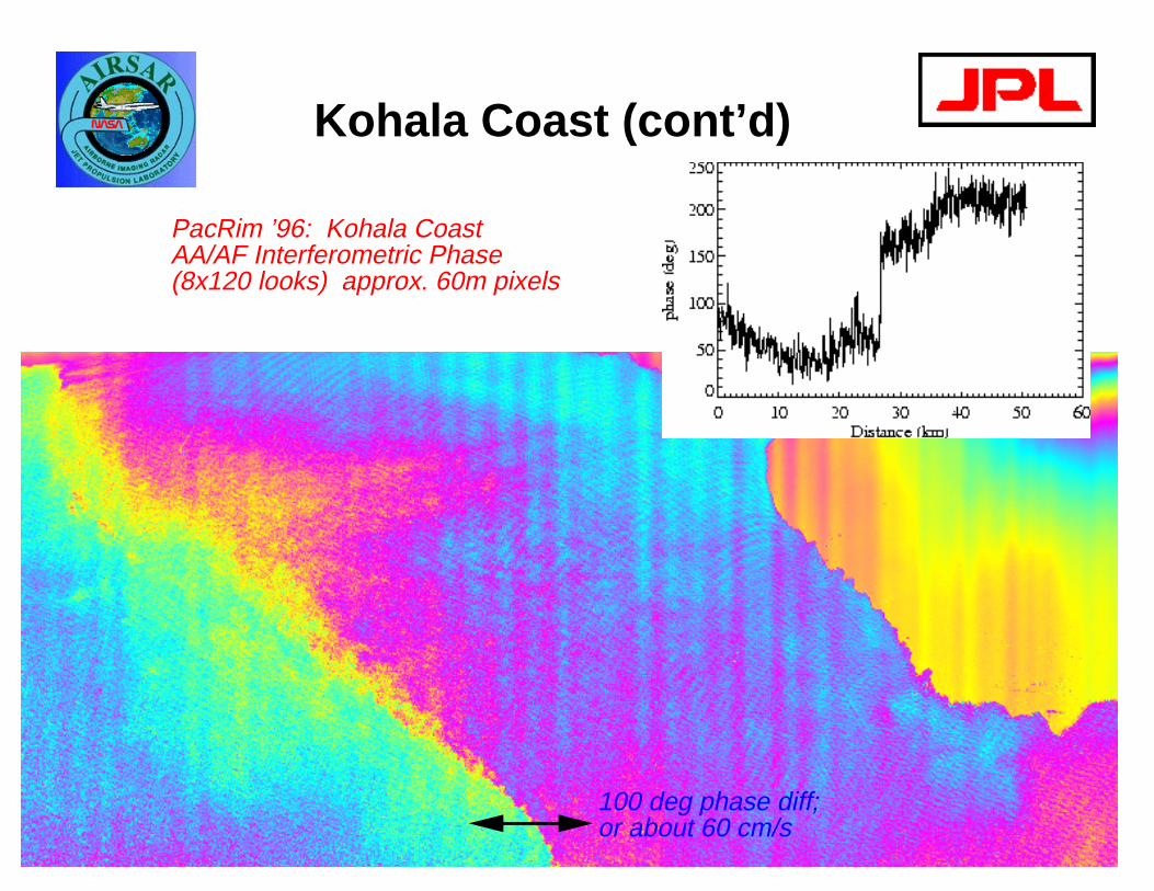
Kohala Coast (cont’d)

PacRim ’96: Kohala Coast AA/AF Interferometric Phase (8x120 looks) approx. 60m pixels

100 deg phase diff;or about 60 cm/s

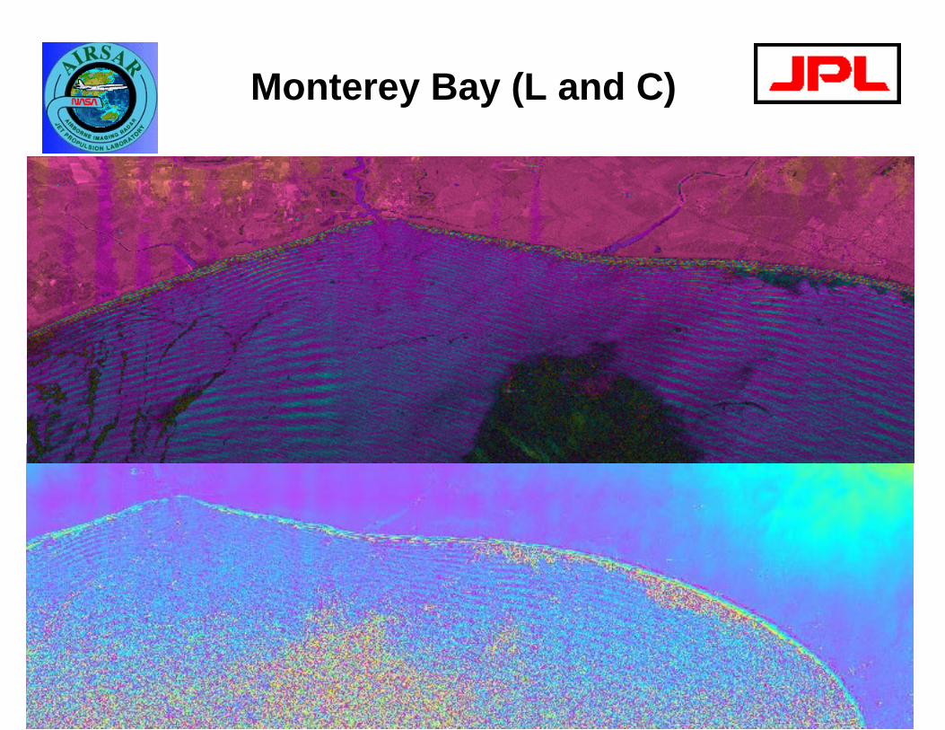
Monterey Bay (L and C)

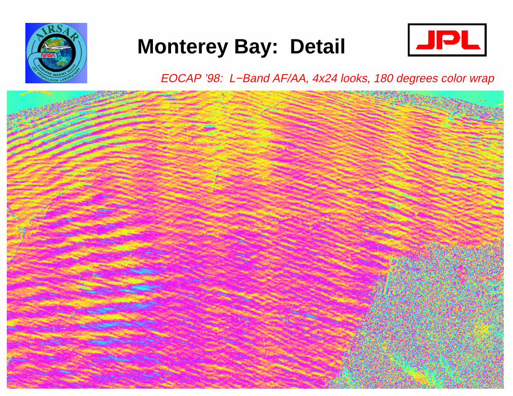
Monterey Bay: DetailEOCAP ’98: L−Band AF/AA, 4x24 looks, 180 degrees color wrap

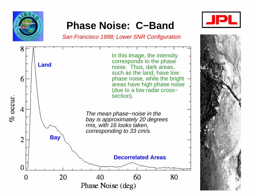
Phase Noise: C−BandSan Francisco 1998; Lower SNR Configuration

In this image, the intensitycorresponds to the phasenoise. Thus, dark areas,such as the land, have lowphase noise, while the brightareas have high phase noise(due to a low radar cross−section).

Land

Bay

Decorrelated Areas

The mean phase−noise in thebay is approximately 20 degreesrms, with 16 looks taken, corresponding to 33 cm/s.

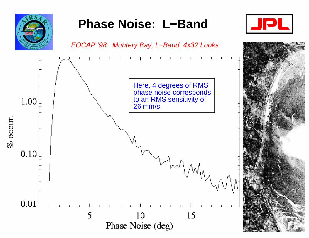
Phase Noise: L−Band

EOCAP ’98: Montery Bay, L−Band, 4x32 Looks

Here, 4 degrees of RMSphase noise correspondsto an RMS sensitivity of 26 mm/s.

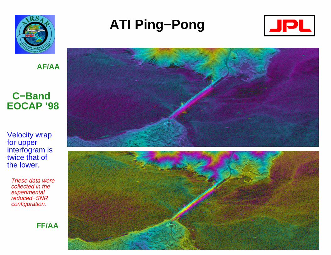
ATI Ping−Pong

Velocity wrapfor upperinterfogram istwice that ofthe lower.

AF/AA

FF/AA

C−BandEOCAP ’98

These data werecollected in theexperimentalreduced−SNRconfiguration.

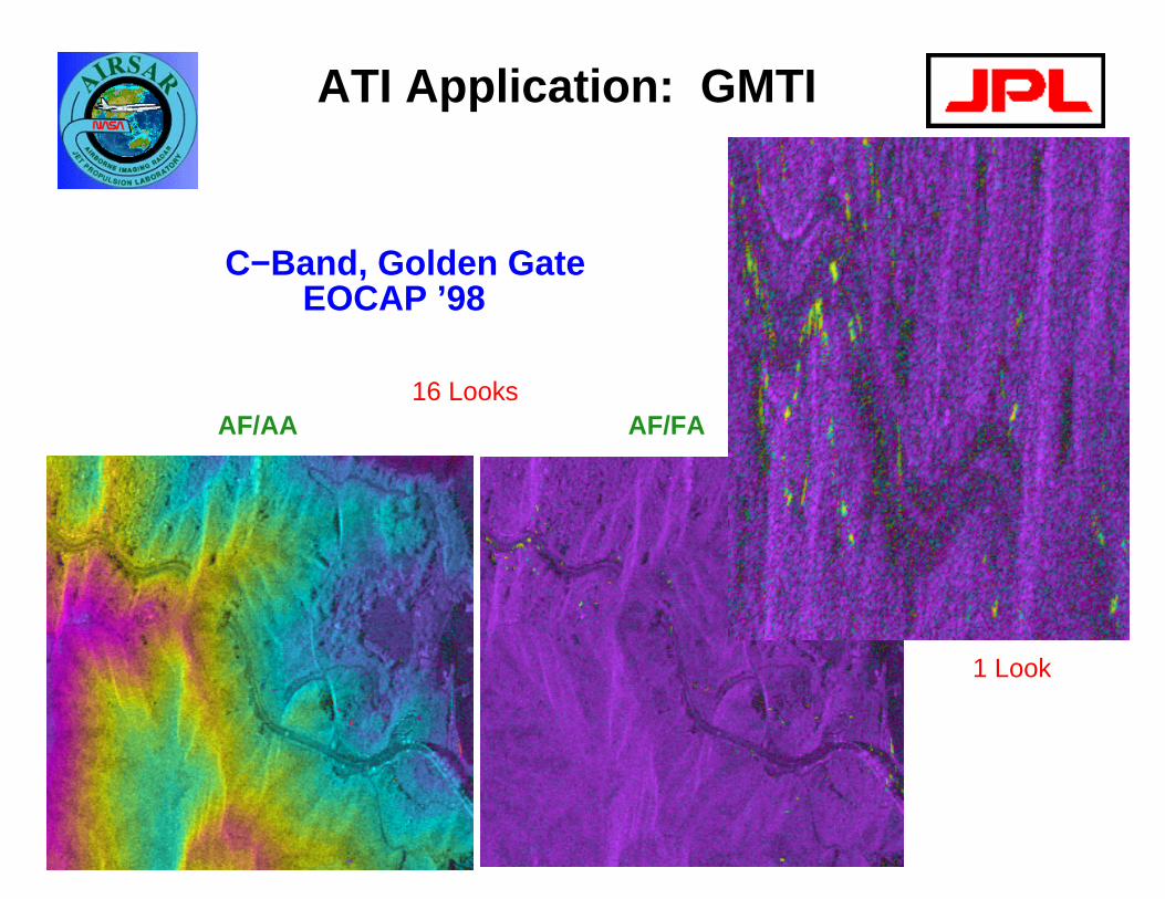
ATI Application: GMTI

C−Band, Golden Gate EOCAP ’98

AF/AA AF/FA16 Looks

1 Look

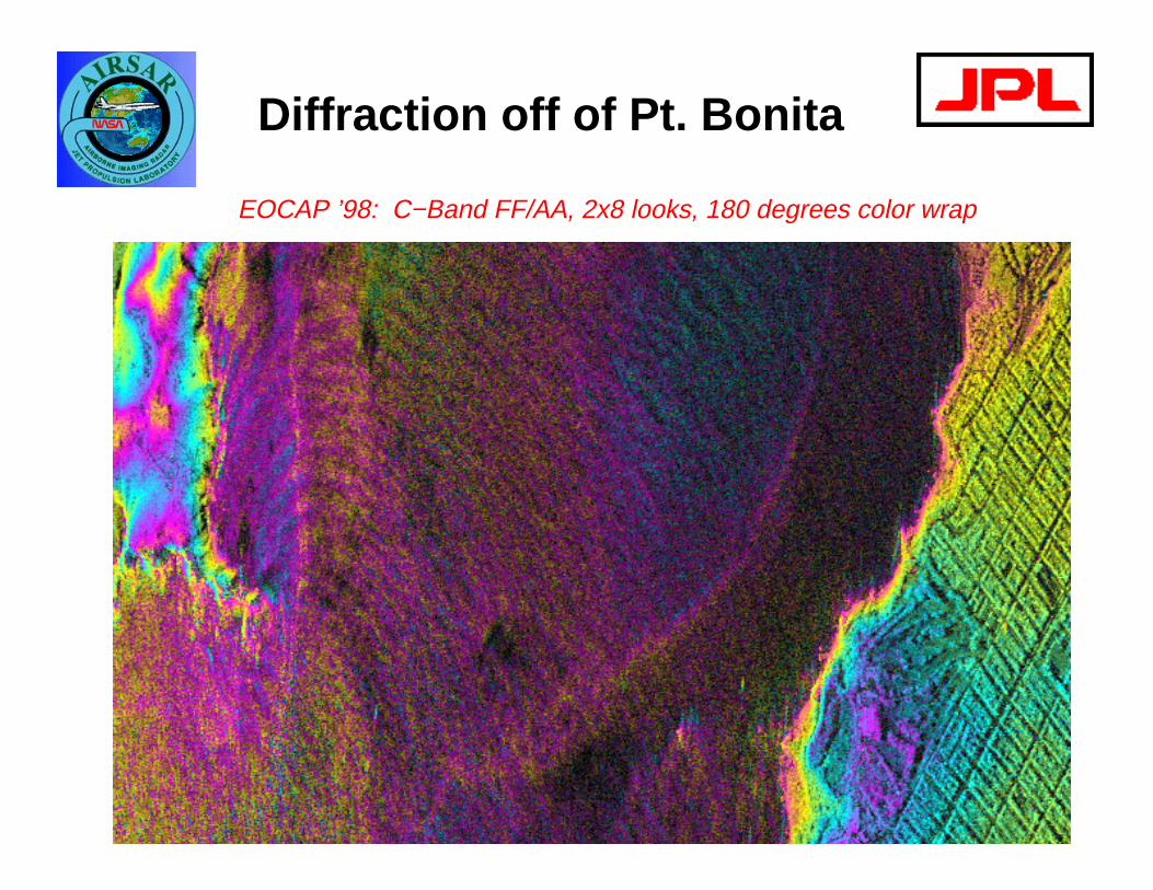
Diffraction off of Pt. Bonita

EOCAP ’98: C−Band FF/AA, 2x8 looks, 180 degrees color wrap

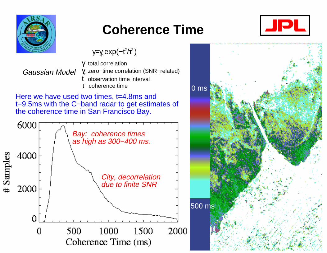
Coherence Time

0 ms

500 ms

Bay: coherence timesas high as 300−400 ms.

City, decorrelationdue to finite SNR

Here we have used two times, t=4.8ms and t=9.5ms with the C−band radar to get estimates of the coherence time in San Francisco Bay.

γ=γ exp(−t /τ )n2 2

Gaussian Modelγ total correlationγ zero−time correlation (SNR−related)t observation time intervalτ coherence time

n

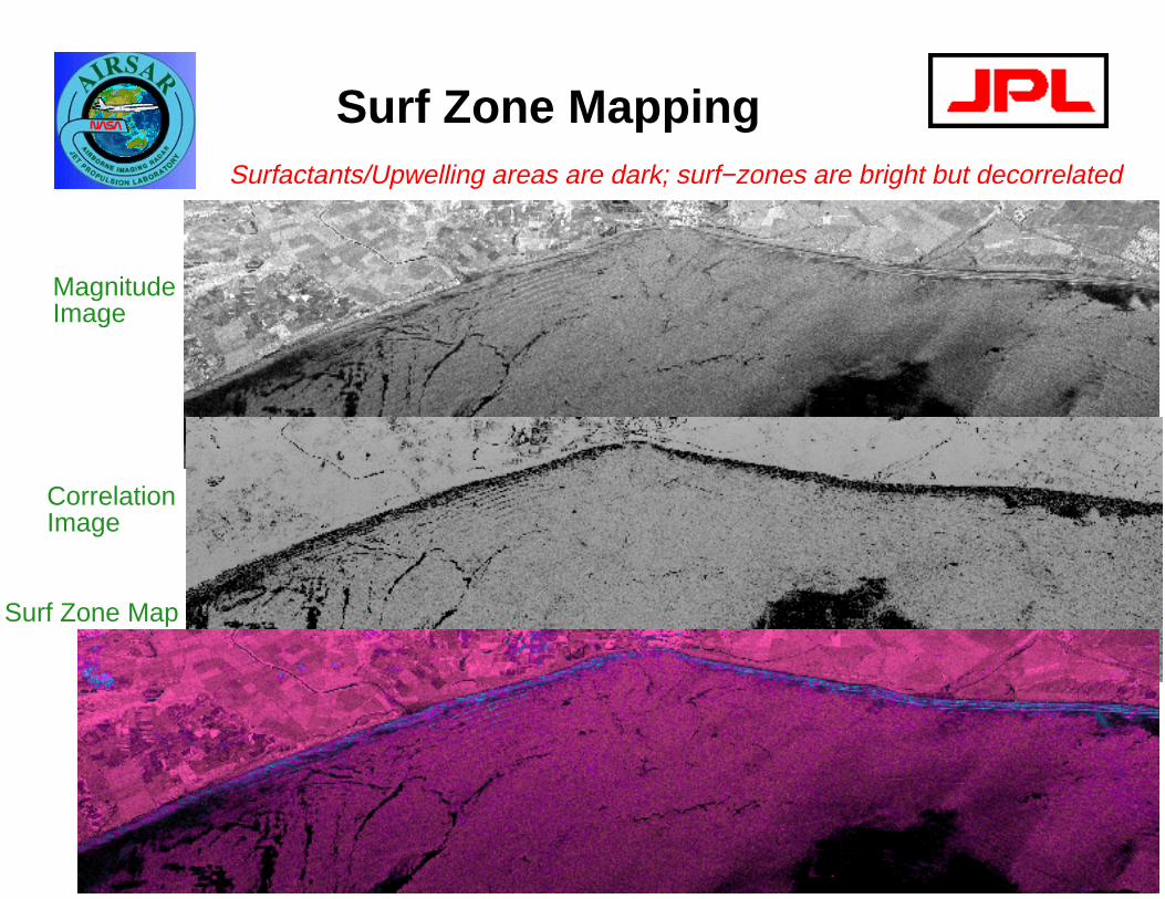
Surf Zone Mapping

MagnitudeImage

CorrelationImage

Surf Zone Map

Surfactants/Upwelling areas are dark; surf−zones are bright but decorrelated

ATI Status at AIRSAR

Processor is functional, ported to several platforms.

Calibration in progress: baseline and delays look good.

Example ATI dataset available before Christmas 1999.

Future: Fully polarimetric C−band ATI (data acquired)

Simultaneous XTI/ATI (data acquired)

Vector ATI (algorithm development)