Alignment-free sequence comparison

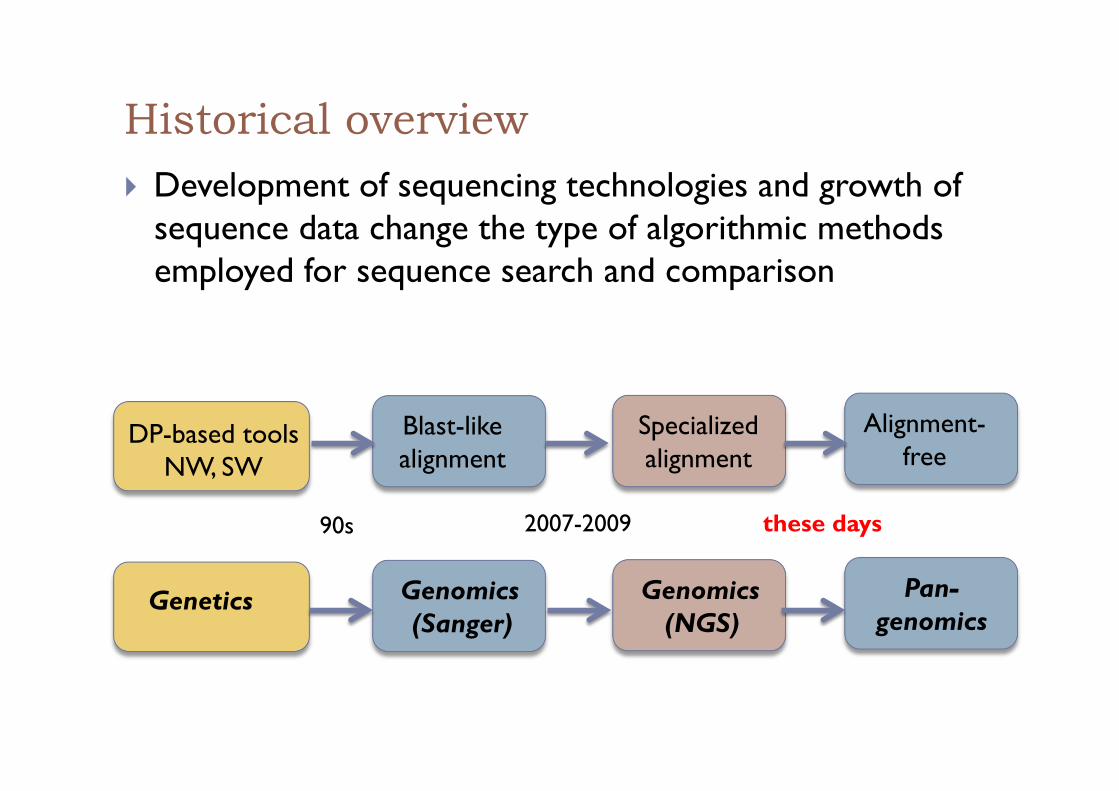
Historical overview !  Development of sequencing technologies and growth of

sequence data change the type of algorithmic methods employed for sequence search and comparison

Genetics

DP-based tools NW, SW

Blast-like alignment

Genomics (Sanger)

Specialized alignment

Genomics (NGS)

Alignment-free

Pan-genomics

2007-2009 90s these days

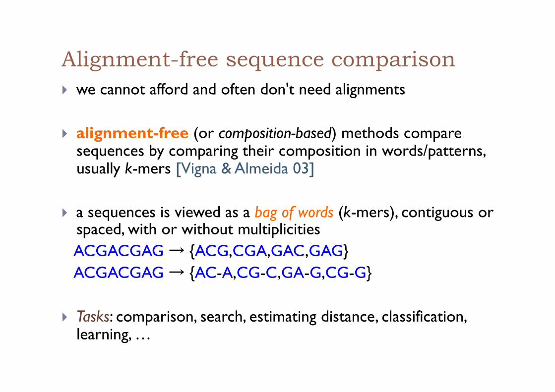
Alignment-free sequence comparison !  we cannot afford and often don't need alignments

!  alignment-free (or composition-based) methods compare sequences by comparing their composition in words/patterns, usually k-mers [Vigna & Almeida 03]

!  a sequences is viewed as a bag of words (k-mers), contiguous or spaced, with or without multiplicities

ACGACGAG → {ACG,CGA,GAC,GAG} ACGACGAG → {AC-A,CG-C,GA-G,CG-G}

!  Tasks: comparison, search, estimating distance, classification, learning, …

Locality-sensitive hashing (LSH)

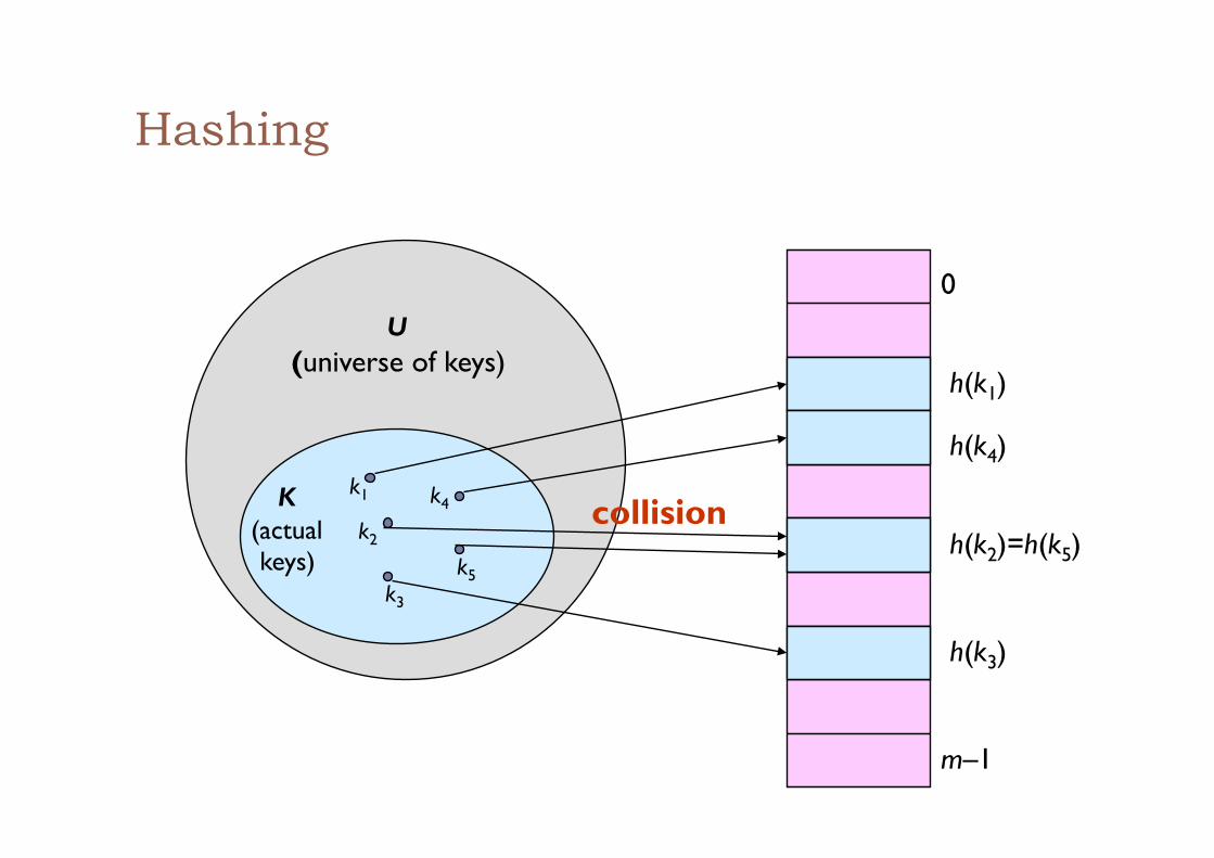
Hashing

0

m–1

h(k1)

h(k4)

h(k2)=h(k5)

h(k3)

U (universe of keys)

K (actual keys)

k1

k2

k3

k5

k4 collision

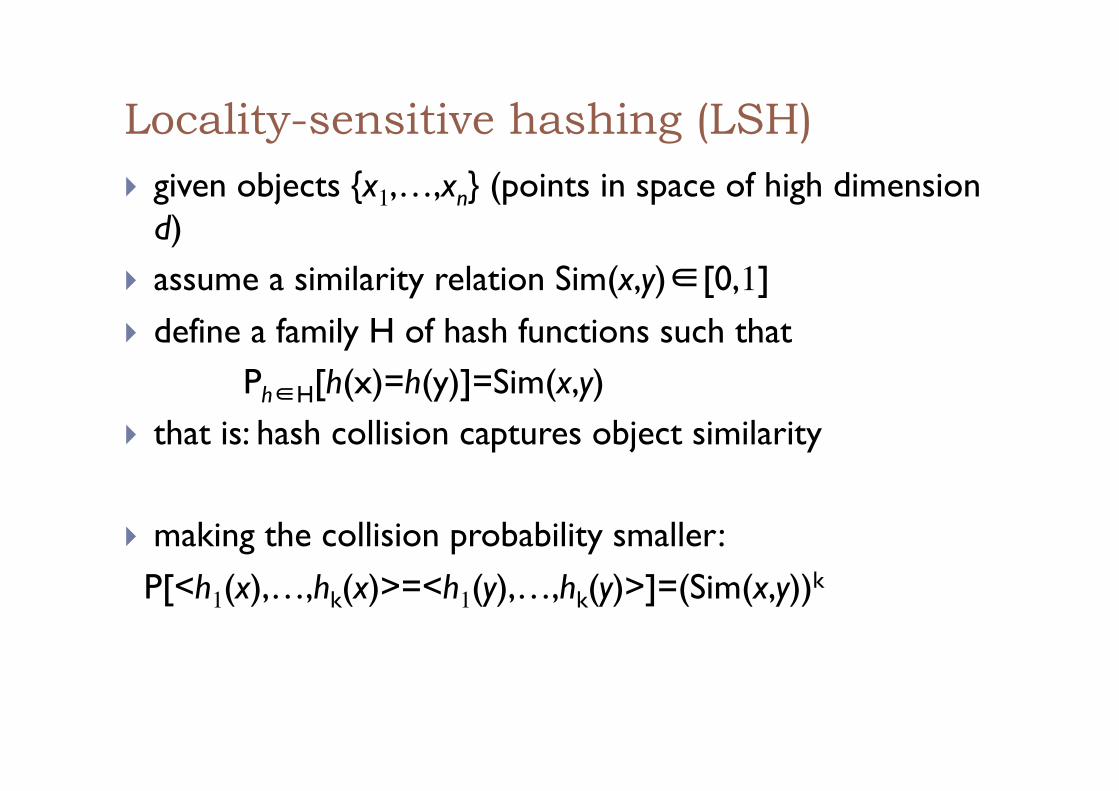
Locality-sensitive hashing (LSH) !  given objects {x1,…,xn} (points in space of high dimension

d) !  assume a similarity relation Sim(x,y)∈[0,1] !  define a family H of hash functions such that Ph∈H[h(x)=h(y)]=Sim(x,y) !  that is: hash collision captures object similarity

Locality-sensitive hashing (LSH) !  given objects {x1,…,xn} (points in space of high dimension

d) !  assume a similarity relation Sim(x,y)∈[0,1] !  define a family H of hash functions such that Ph∈H[h(x)=h(y)]=Sim(x,y) !  that is: hash collision captures object similarity

!  making the collision probability smaller: P[<h1(x),…,hk(x)>=<h1(y),…,hk(y)>]=(Sim(x,y))k

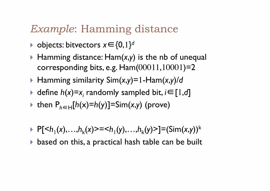
Example: Hamming distance !  objects: bitvectors x∈{0,1}d

!  Hamming distance: Ham(x,y) is the nb of unequal corresponding bits, e.g. Ham(00011,10001)=2

!  Hamming similarity Sim(x,y)=1-Ham(x,y)/d !  define h(x)=xi randomly sampled bit, i∈[1,d] !  then Ph∈H[h(x)=h(y)]=Sim(x,y) (prove)

!  P[<h1(x),…,hk(x)>=<h1(y),…,hk(y)>]=(Sim(x,y))k !  based on this, a practical hash table can be built

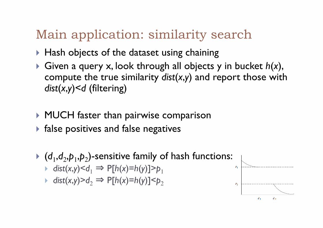
Main application: similarity search !  Hash objects of the dataset using chaining !  Given a query x, look through all objects y in bucket h(x),

compute the true similarity dist(x,y) and report those with dist(x,y)<d (filtering)

!  MUCH faster than pairwise comparison !  false positives and false negatives

!  (d1,d2,p1,p2)-sensitive family of hash functions: !  dist(x,y)<d1 ⇒ P[h(x)=h(y)]>p1 !  dist(x,y)>d2 ⇒ P[h(x)=h(y)]<p2

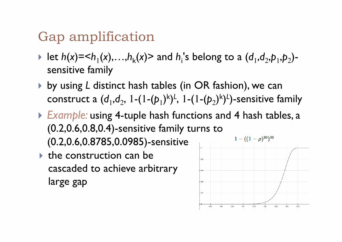
Gap amplification !  let h(x)=<h1(x),…,hk(x)> and hi's belong to a (d1,d2,p1,p2)-

sensitive family !  by using L distinct hash tables (in OR fashion), we can

construct a (d1,d2, 1-(1-(p1)k)L, 1-(1-(p2)k)L)-sensitive family !  Example: using 4-tuple hash functions and 4 hash tables, a

(0.2,0.6,0.8,0.4)-sensitive family turns to (0.2,0.6,0.8785,0.0985)-sensitive

!  the construction can be cascaded to achieve arbitrary large gap

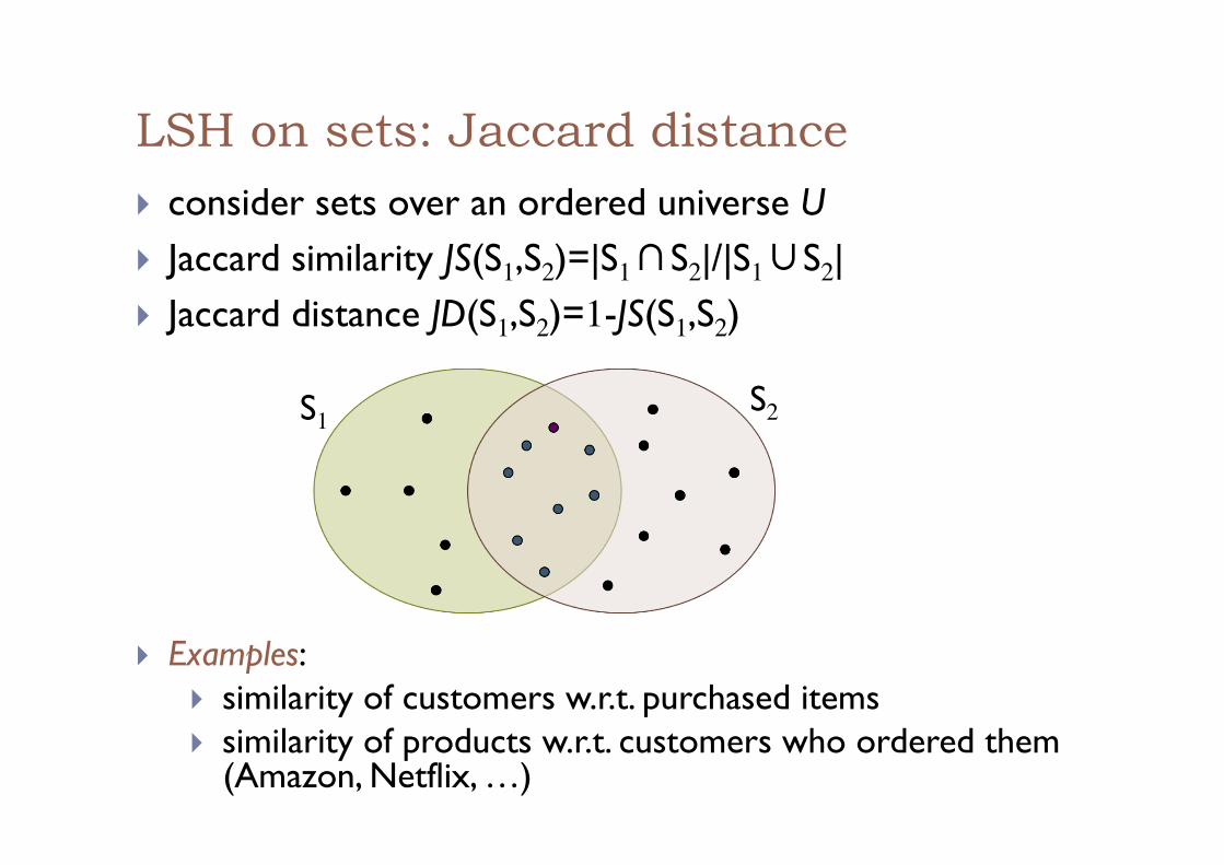
LSH on sets: Jaccard distance !  consider sets over an ordered universe U !  Jaccard similarity JS(S1,S2)=|S1∩S2|/|S1∪S2| !  Jaccard distance JD(S1,S2)=1-JS(S1,S2)

S1 S2

!  Examples: !  similarity of customers w.r.t. purchased items !  similarity of products w.r.t. customers who ordered them

(Amazon, Netflix, …)

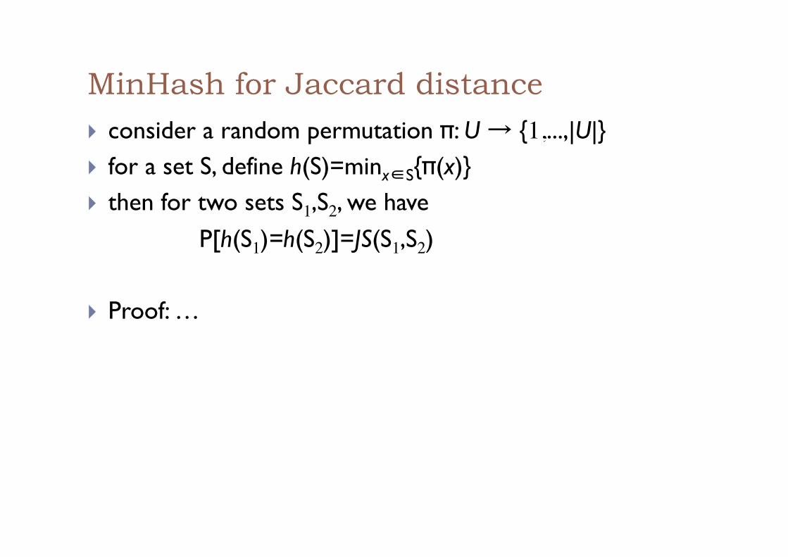
MinHash for Jaccard distance !  consider a random permutation π: U → {1,...,|U|} !  for a set S, define h(S)=minx∈S{π(x)} !  then for two sets S1,S2, we have P[h(S1)=h(S2)]=JS(S1,S2)

!  Proof: …

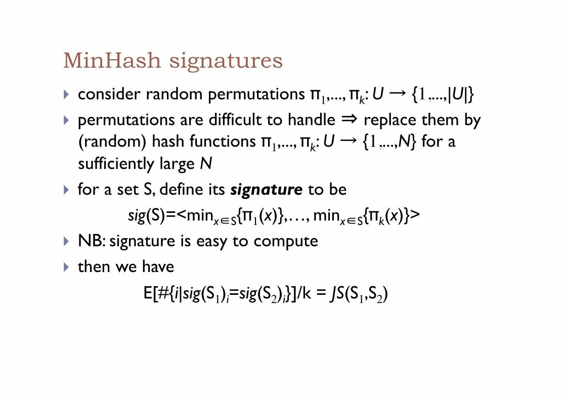
MinHash signatures !  consider random permutations π1,..., πk: U → {1,...,|U|} !  permutations are difficult to handle ⇒ replace them by

(random) hash functions π1,..., πk: U → {1,...,N} for a sufficiently large N

!  for a set S, define its signature to be sig(S)=<minx∈S{π1(x)},…, minx∈S{πk(x)}> !  NB: signature is easy to compute !  then we have E[#{i|sig(S1)i=sig(S2)i}]/k = JS(S1,S2)

MinHash: toy example S1={0,3}, S2={2}, S3={1,3,4}, S4={0,2,3} π1(x)=(x+1) mod 5π2(x)=(3x+1) mod 5sig(S1)=<1,0>, sig(S2)=<3,2>, sig(S3)=<0,0>, sig(S4)=<1,0>

Then JS(S1,S4) estimated to 1 (true answer 2/3) JS(S1,S3) estimated to 1/2 (true answer 1/4) JS(S3,S4) estimated to 1/2 (true answer 1/5) JS(S1,S2) estimated to 0 (true answer 0)

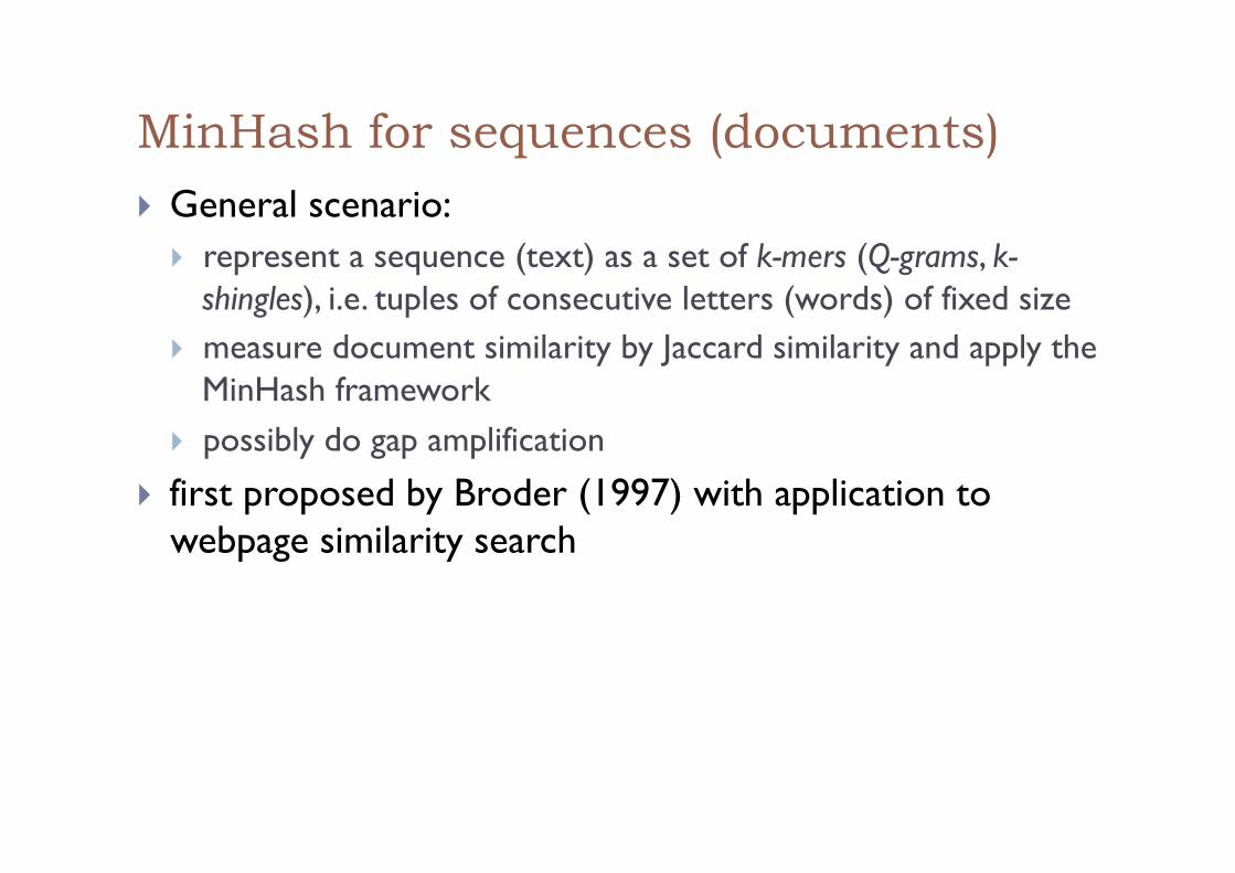
MinHash for sequences (documents) !  General scenario:

!  represent a sequence (text) as a set of k-mers (Q-grams, k-shingles), i.e. tuples of consecutive letters (words) of fixed size

!  measure document similarity by Jaccard similarity and apply the MinHash framework

!  possibly do gap amplification

!  first proposed by Broder (1997) with application to webpage similarity search

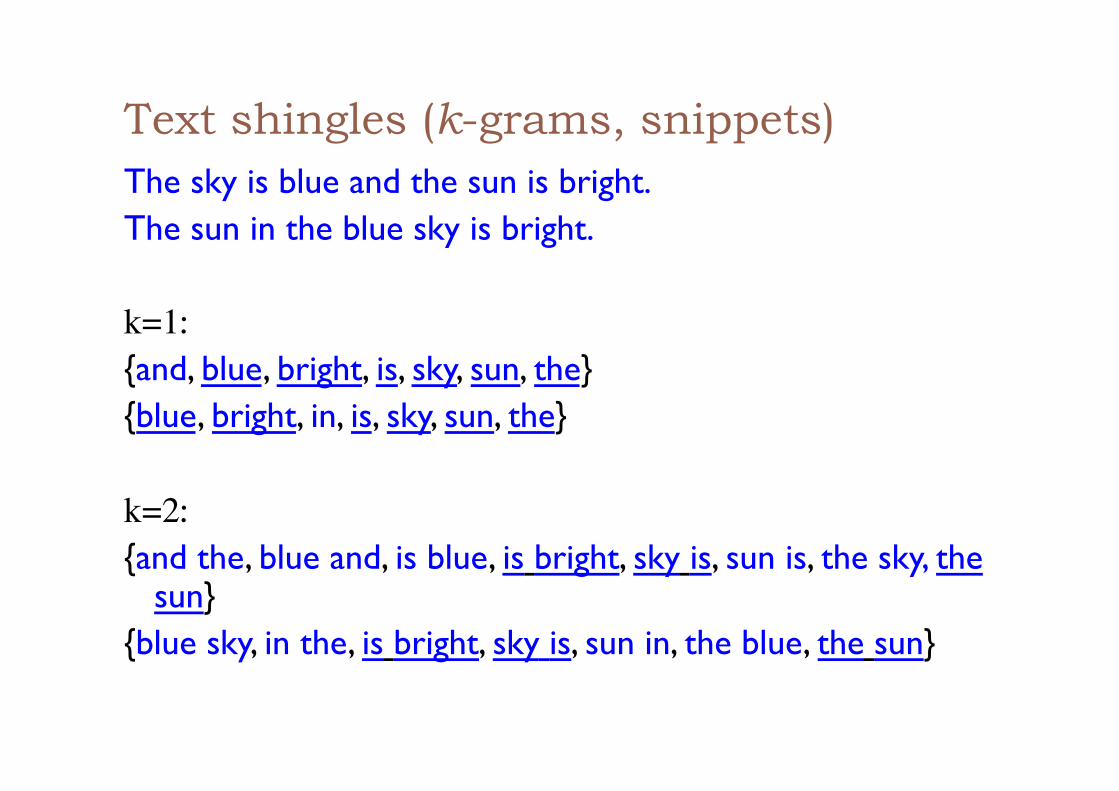
Text shingles (k-grams, snippets) The sky is blue and the sun is bright. The sun in the blue sky is bright.

k=1: {and, blue, bright, is, sky, sun, the} {blue, bright, in, is, sky, sun, the}

k=2: {and the, blue and, is blue, is bright, sky is, sun is, the sky, the

sun} {blue sky, in the, is bright, sky is, sun in, the blue, the sun}

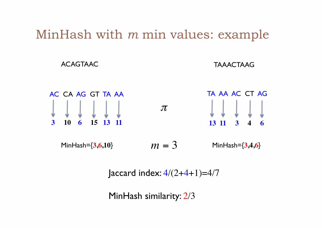
MinHash with m min values: example

ACAGTAAC TAAACTAAG

3 10 6 15 13 11 13 11 3 4 6

AC CA AG GT TA AA TA AA AC CT AG

€

π

MinHash={3,6,10} MinHash={3,4,6}

Jaccard index: 4/(2+4+1)=4/7

MinHash similarity: 2/3€

m = 3

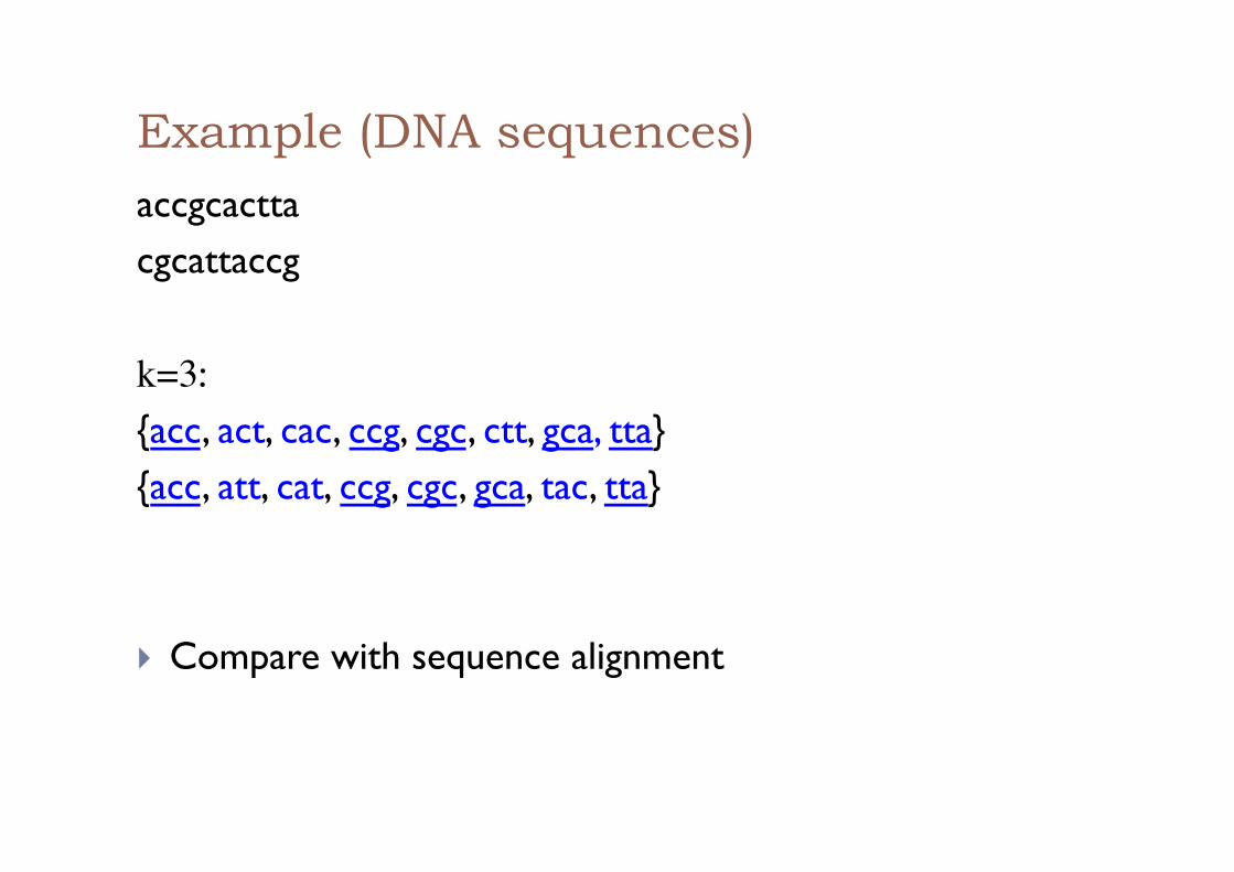
Example (DNA sequences) accgcactta cgcattaccg

k=3: {acc, act, cac, ccg, cgc, ctt, gca, tta} {acc, att, cat, ccg, cgc, gca, tac, tta}

!  Compare with sequence alignment

Features of MinHash !  Simple! easy to compute! !  Can be combined with spaced seeds !  Easy to maintain for growing datasets !  Size (m) does not depend on the size of the dataset !  Suitable for comparing datasets of (roughly) the same size !  Low level of false positives ("accidental similarity")

!  Example: fingerprints of 400 32-bit hash values (k=16) are sufficient to discriminate microbial genomes (a few Mb)

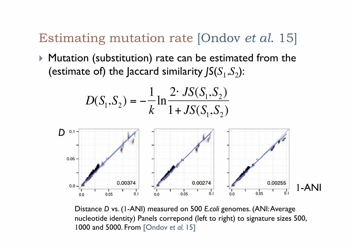
Estimating mutation rate [Ondov et al. 15]

!  Mutation (substitution) rate can be estimated from the (estimate of) the Jaccard similarity JS(S1,S2):

€

D(S1,S2) = −1kln 2⋅ JS(S1,S2)1+ JS(S1,S2)

0.0 0.05 0.1 0.0 0.05 0.1 0.0 0.05 0.1

Distance D vs. (1-ANI) measured on 500 E.coli genomes. (ANI: Average nucleotide identity) Panels correpond (left to right) to signature sizes 500, 1000 and 5000. From [Ondov et al. 15]

D

1-ANI

Examples of application [Ondov et al. 15]

!  clustering of 54,000 NCBI genomes (entire RefSeq, 618Gbp) in 33 CPU h using 1,000-valued hashes. Resulting hashes: 93MB

!  (real-time) matching a sequencing data against a "sketched" database

!  scalable clustering of hundreds of metagenomic samples by composition: analysis of 10TB of sequence data using 10,000-valued hashes (k = 21)

Bonus: Bloom filters

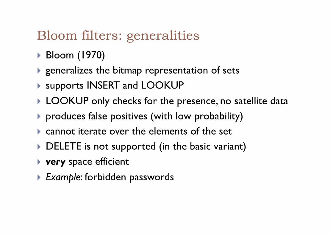
Bloom filters: generalities !  Bloom (1970) !  generalizes the bitmap representation of sets !  supports INSERT and LOOKUP !  LOOKUP only checks for the presence, no satellite data !  produces false positives (with low probability) !  cannot iterate over the elements of the set !  DELETE is not supported (in the basic variant) !  very space efficient !  Example: forbidden passwords

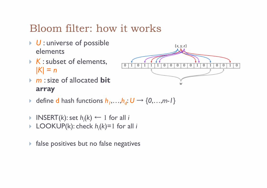
Bloom filter: how it works !  U : universe of possible

elements !  K : subset of elements,

|K| = n !  m : size of allocated bit

array !  define d hash functions h1,…,hd: U → {0,…,m-1}

!  INSERT(k): set hi(k) ← 1 for all i !  LOOKUP(k): check hi(k)=1 for all i

!  false positives but no false negatives

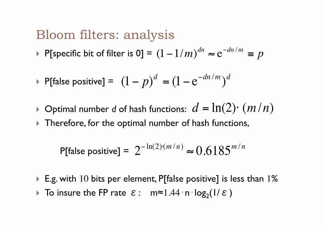
Bloom filters: analysis !  P[specific bit of filter is 0] =

!  P[false positive] =

!  Optimal number d of hash functions: !  Therefore, for the optimal number of hash functions,

P[false positive] =

!  E.g. with 10 bits per element, P[false positive] is less than 1% !  To insure the FP rate ε: m≈1.44⋅n⋅log2(1/ε)

€

(1−1/m)dn ≈ e−dn /m ≡ p

€

(1− p)d = (1− e−dn /m )d

€

d = ln(2)⋅ (m /n)

€

2− ln(2)⋅(m / n ) ≈ 0.6185m / n

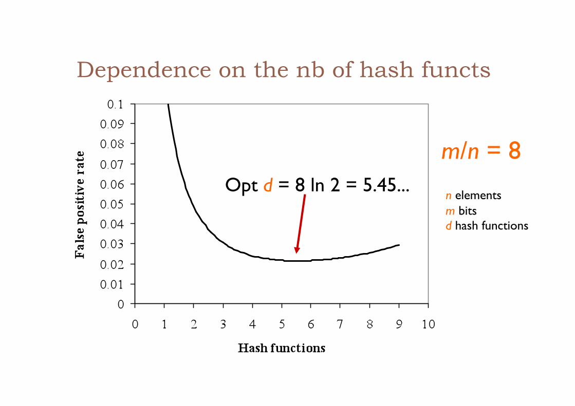
Dependence on the nb of hash functs

m/n = 8

Opt d = 8 ln 2 = 5.45... n elements m bits d hash functions

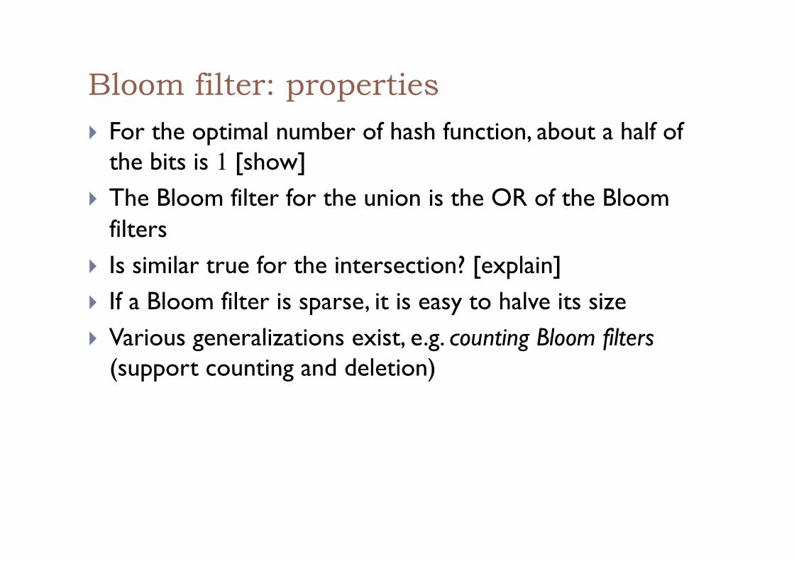
Bloom filter: properties !  For the optimal number of hash function, about a half of

the bits is 1 [show]!  The Bloom filter for the union is the OR of the Bloom

filters !  Is similar true for the intersection? [explain] !  If a Bloom filter is sparse, it is easy to halve its size !  Various generalizations exist, e.g. counting Bloom filters

(support counting and deletion)

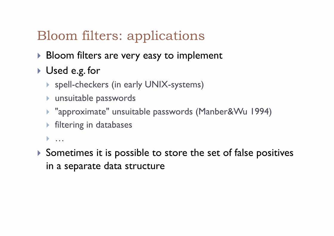
Bloom filters: applications !  Bloom filters are very easy to implement !  Used e.g. for

!  spell-checkers (in early UNIX-systems) !  unsuitable passwords !  "approximate" unsuitable passwords (Manber&Wu 1994) !  filtering in databases !  …

!  Sometimes it is possible to store the set of false positives in a separate data structure