Al ParkerSeptember 14, 2010

Drawing samples from high dimensional Gaussians using

polynomials

• Colin Fox, Physics, University of Otago

• New Zealand Institute of Mathematics, University of Auckland

• Center for Biofilm Engineering, , Bozeman

Acknowledgements

2

22

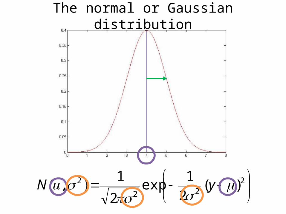
2 )(2

1exp

2

1),(

yN

The normal or Gaussian distribution

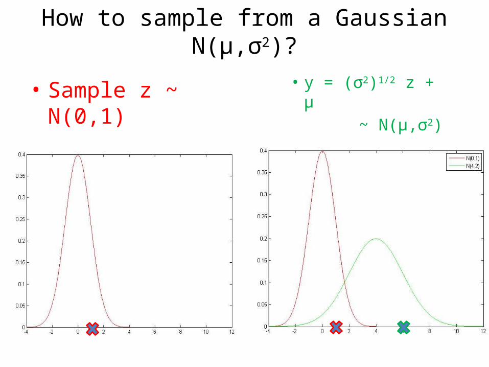
• y = (σ2)1/2 z + µ ~ N(µ,σ2)

How to sample from a Gaussian N(µ,σ2)?

• Sample z ~ N(0,1)

)()(

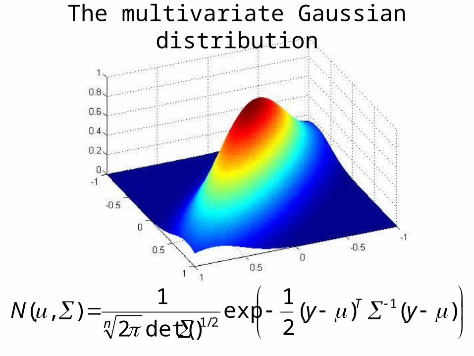
2

1exp

)det(2

1),( 1

2/1

yyN T

n

The multivariate Gaussian distribution

T

T

T

T

n

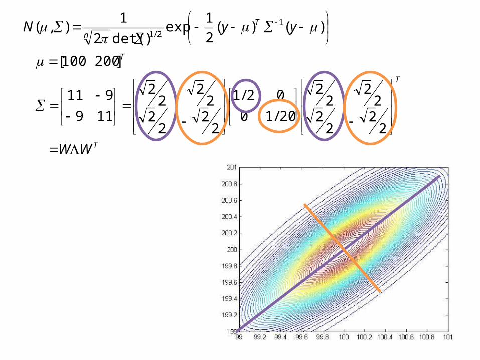
WW

yyN

22

22

22

22

20/10

02/1

22

22

22

22

119

911

]200100[

)()(2

1exp

)det(2

1),( 1

2/1

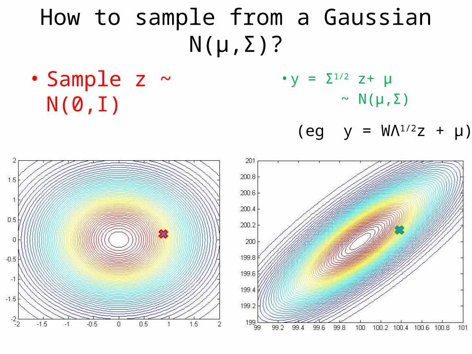
• y = Σ1/2 z+ µ ~ N(µ,Σ)

How to sample from a Gaussian N(µ,Σ)?

• Sample z ~ N(0,I)

(eg y = WΛ1/2z + µ)

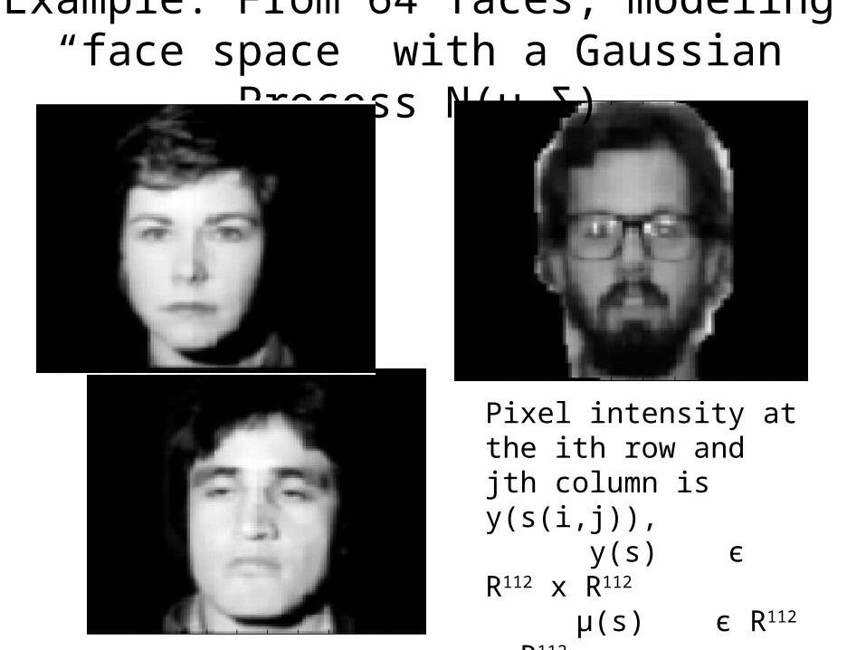
Example: From 64 faces, modeling “face space” with a Gaussian Process N(μ,Σ)

Pixel intensity at the ith row and jth column is y(s(i,j)), y(s) є R112 x R112

μ(s) є R112 x R112

Σ(s,s) є R12544 x R12544

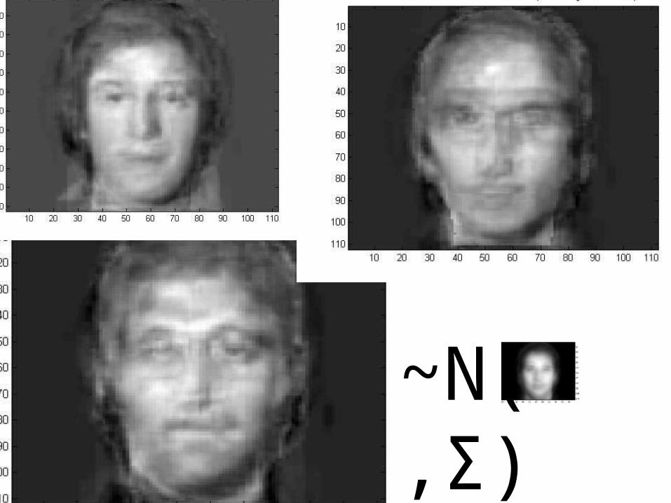
~N( ,Σ)

How to estimate μ,Σ for N(μ,Σ)?

• MLE/BLUE (least squares)• MVQUE• Use a Bayesian Posterior via MCMC

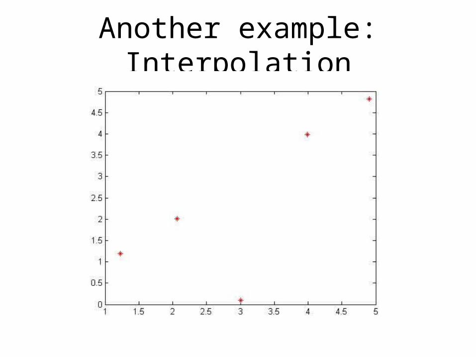
Another example: Interpolation

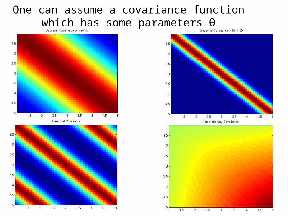
One can assume a covariance function which has some parameters θ

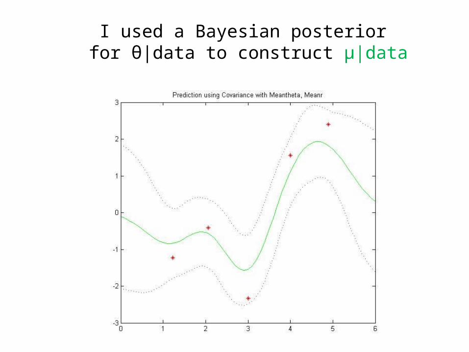
I used a Bayesian posterior for θ|data to construct μ|data

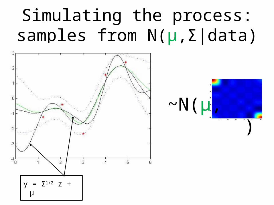
Simulating the process:samples from N(μ,Σ|data)

y = Σ1/2 z + µ

~N(μ, )

Gaussian Processes modeling global ozone

Cressie and Johannesson, Fixed rank krigging for very large spatial datasets, 2006

Gaussian Processes modeling global ozone

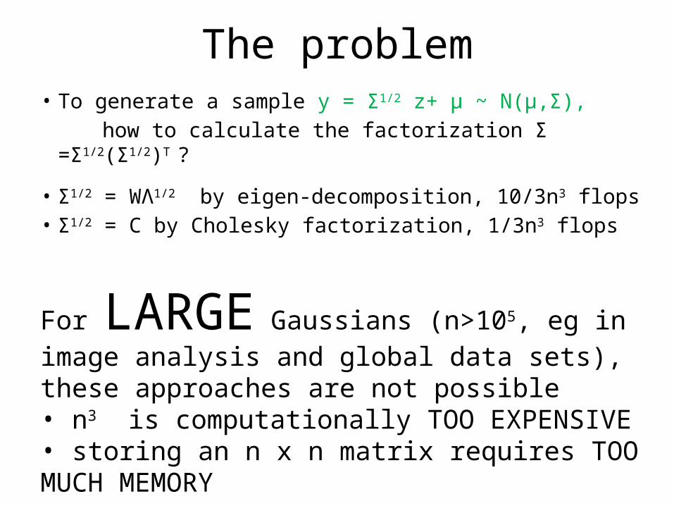
The problem• To generate a sample y = Σ1/2 z+ µ ~ N(µ,Σ), how to calculate the factorization Σ =Σ1/2(Σ1/2)T ?

• Σ1/2 = WΛ1/2 by eigen-decomposition, 10/3n3 flops• Σ1/2 = C by Cholesky factorization, 1/3n3 flops

For LARGE Gaussians (n>105, eg in image analysis and global data sets), these approaches are not possible• n3 is computationally TOO EXPENSIVE • storing an n x n matrix requires TOO MUCH MEMORY

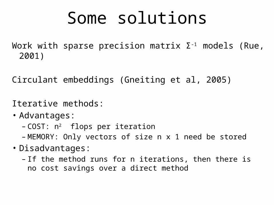
Some solutions

Work with sparse precision matrix Σ-1 models (Rue, 2001)

Circulant embeddings (Gneiting et al, 2005)

Iterative methods:• Advantages:

– COST: n2 flops per iteration– MEMORY: Only vectors of size n x 1 need be stored

• Disadvantages:– If the method runs for n iterations, then there is no cost savings over

a direct method

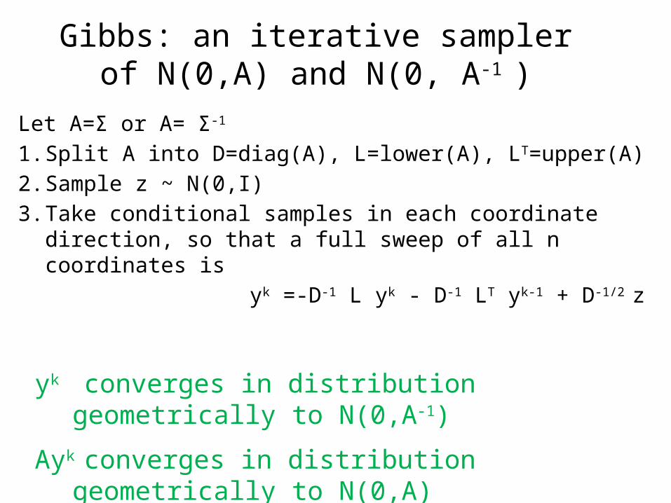
Gibbs: an iterative sampler of N(0,A) and N(0, A-1 )

Let A=Σ or A= Σ-1

1. Split A into D=diag(A), L=lower(A), LT=upper(A)2. Sample z ~ N(0,I) 3. Take conditional samples in each coordinate

direction, so that a full sweep of all n coordinates is yk =-D-1 L yk - D-1 LT yk-1 + D-1/2 z

yk converges in distribution geometrically to N(0,A-1)

Ayk converges in distribution geometrically to N(0,A)

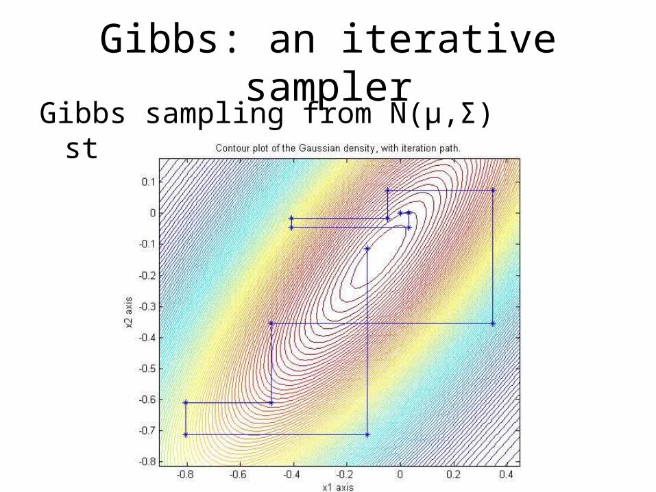
Gibbs: an iterative samplerGibbs sampling from N(µ,Σ) starting from (0,0)

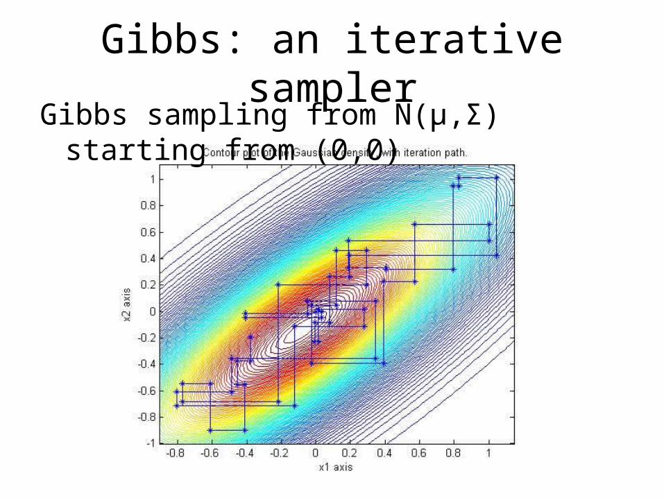
Gibbs: an iterative samplerGibbs sampling from N(µ,Σ) starting from (0,0)

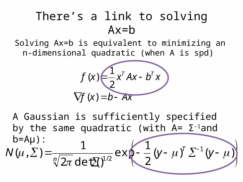
There’s a link to solvingAx=b

Solving Ax=b is equivalent to minimizing an n-dimensional quadratic (when A is spd)

)()(

2

1exp

)det(2

1),( 1

2/1

yyN T

n

Axbxf

xbAxxxf TT

)(2

1)(

A Gaussian is sufficiently specified by the same quadratic (with A= Σ-1and b=Aμ):

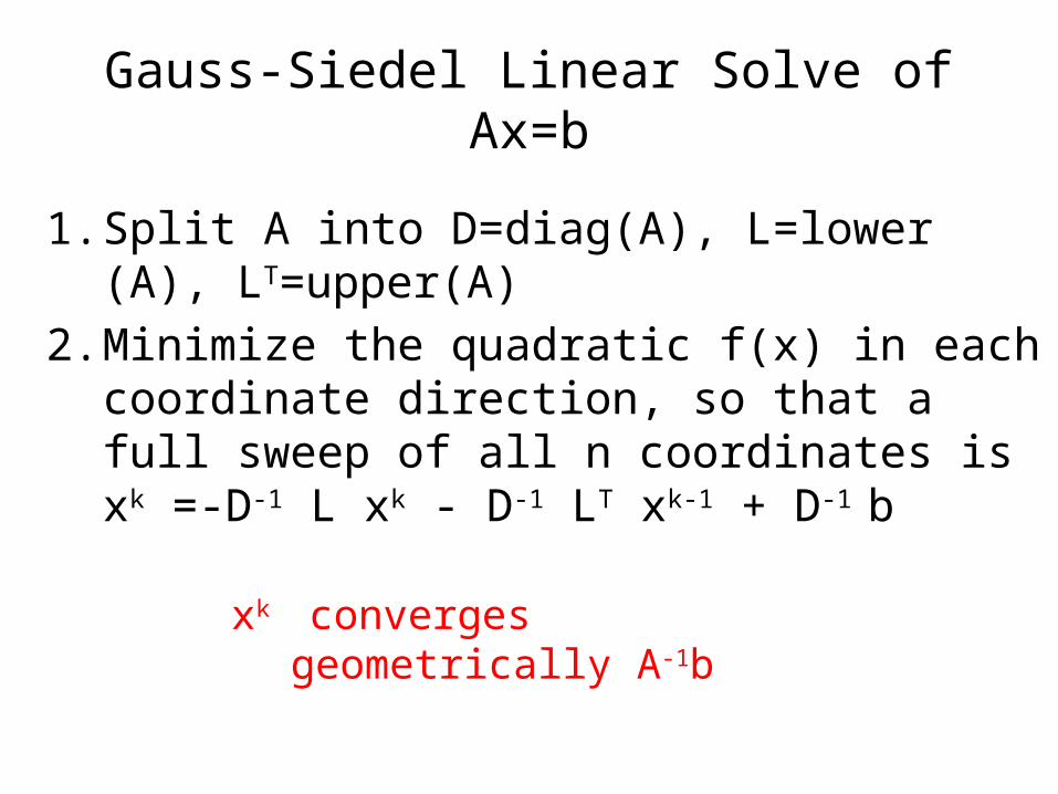
Gauss-Siedel Linear Solve of Ax=b

1. Split A into D=diag(A), L=lower (A), LT=upper(A)2. Minimize the quadratic f(x) in each coordinate

direction, so that a full sweep of all n coordinates is

xk =-D-1 L xk - D-1 LT xk-1 + D-1 b

xk converges geometrically A-1b

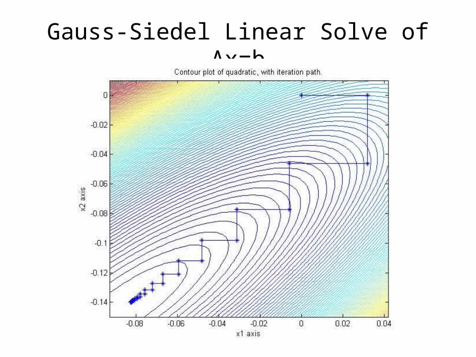
Gauss-Siedel Linear Solve of Ax=b

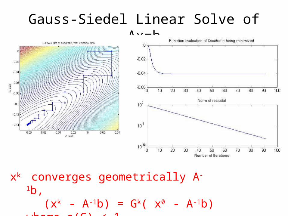
Gauss-Siedel Linear Solve of Ax=b

xk converges geometrically A-1b, (xk - A-1b) = Gk( x0 - A-1b) where ρ(G) < 1

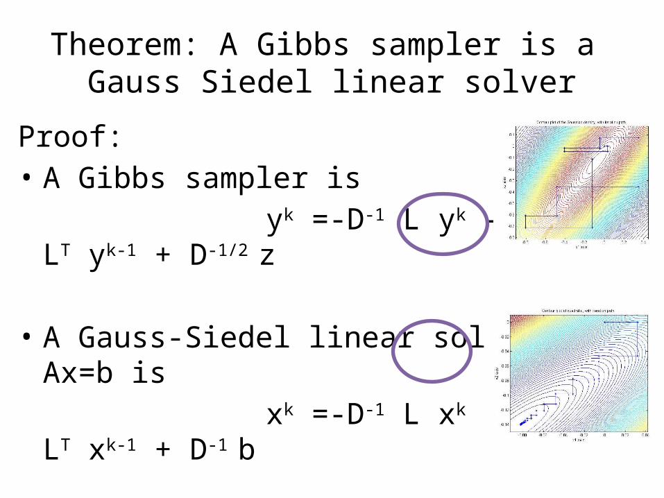
Theorem: A Gibbs sampler is a Gauss Siedel linear solver

Proof: • A Gibbs sampler is yk =-D-1 L yk - D-1 LT yk-1 + D-1/2 z

• A Gauss-Siedel linear solve of Ax=b is xk =-D-1 L xk - D-1 LT xk-1 + D-1 b

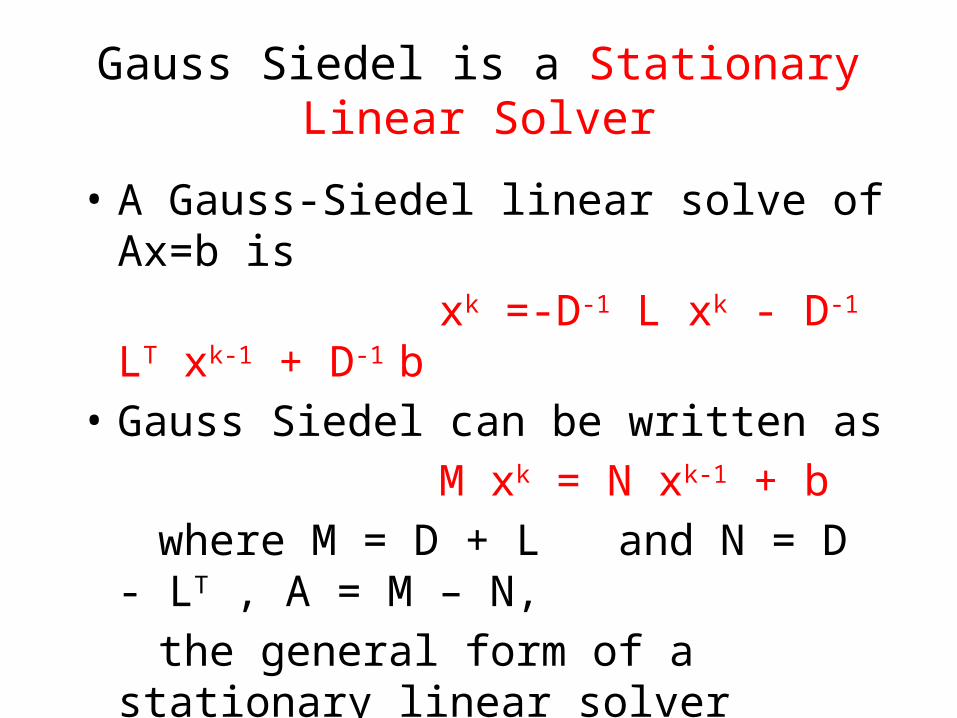
Gauss Siedel is a Stationary Linear Solver

• A Gauss-Siedel linear solve of Ax=b is xk =-D-1 L xk - D-1 LT xk-1 + D-1 b• Gauss Siedel can be written as M xk = N xk-1 + b where M = D + L and N = D - LT , A = M – N, the general form of a stationary linear solver

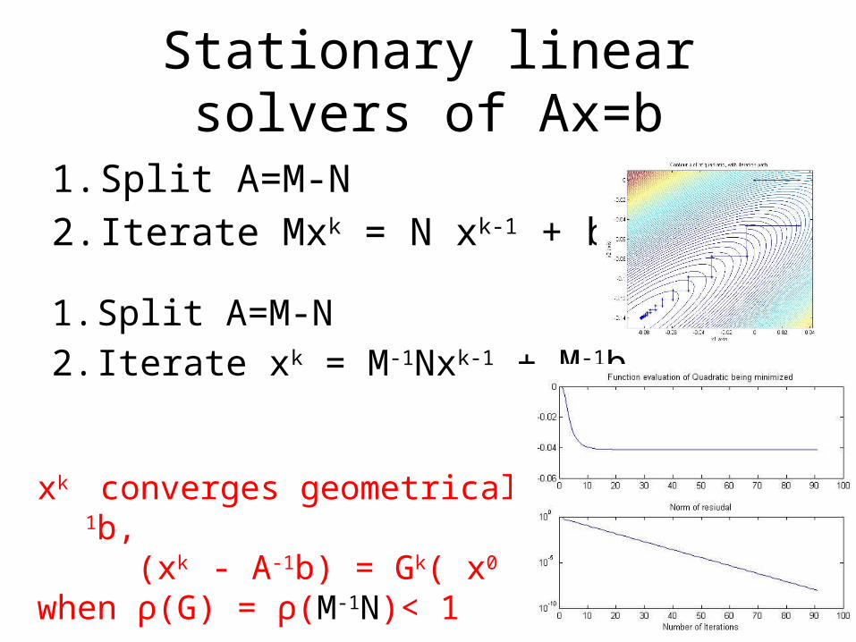
Stationary linear solvers of Ax=b

1. Split A=M-N 2. Iterate Mxk = N xk-1 + b

1. Split A=M-N 2. Iterate xk = M-1Nxk-1 + M-1b = Gxk-1 + M-1b

xk converges geometrically A-1b, (xk - A-1b) = Gk( x0 - A-1b) when ρ(G) = ρ(M-1N)< 1

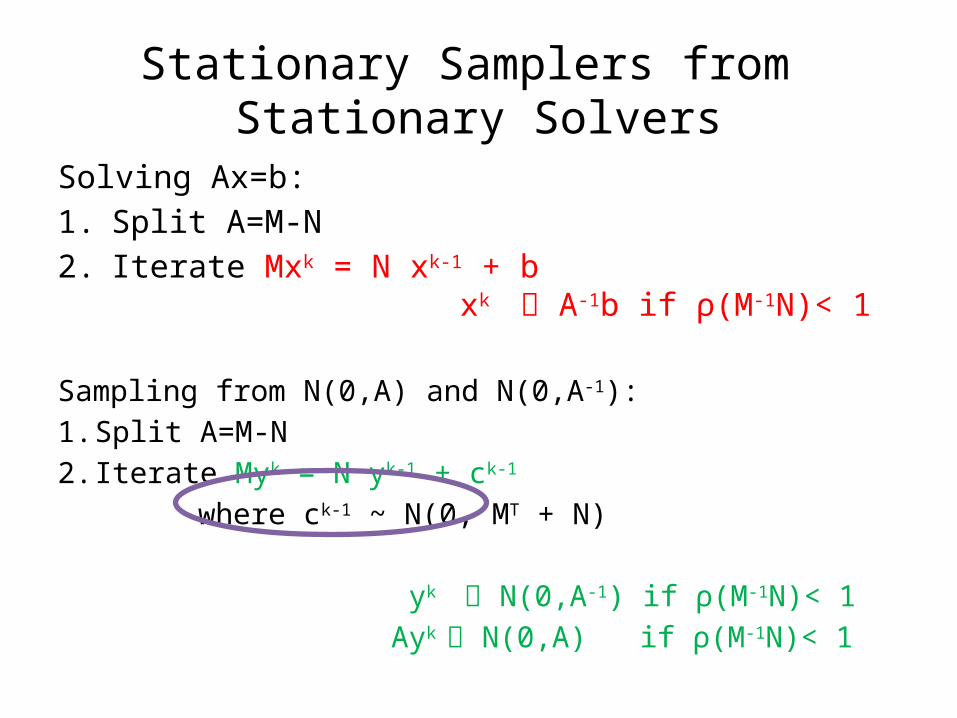
Stationary Samplers from Stationary Solvers

Solving Ax=b:1. Split A=M-N 2. Iterate Mxk = N xk-1 + b xk A-1b if ρ(M-1N)< 1

Sampling from N(0,A) and N(0,A-1):1. Split A=M-N2. Iterate Myk = N yk-1 + ck-1

where ck-1 ~ N(0, MT + N) yk N(0,A-1) if ρ(M-1N)< 1 Ayk N(0,A) if ρ(M-1N)< 1

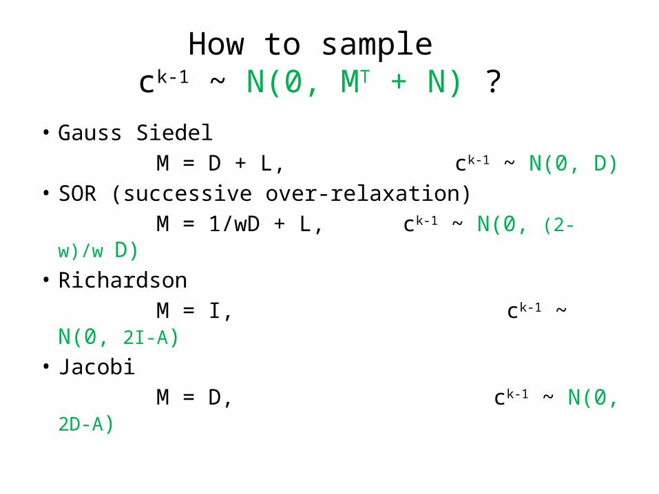
How to sample ck-1 ~ N(0, MT + N) ?

• Gauss Siedel M = D + L, ck-1 ~ N(0, D)• SOR (successive over-relaxation) M = 1/wD + L, ck-1 ~ N(0, (2-w)/w D)• Richardson M = I, ck-1 ~ N(0, 2I-A)• Jacobi M = D, ck-1 ~ N(0, 2D-A)

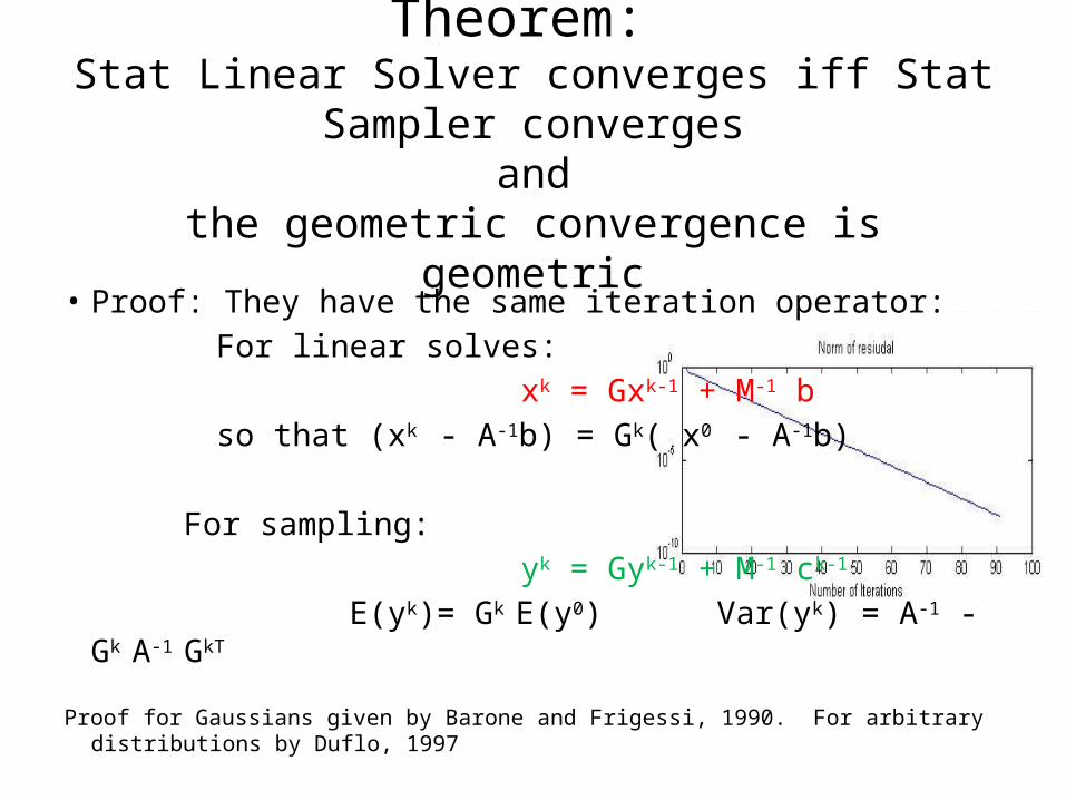
Theorem: Stat Linear Solver converges iff Stat Sampler converges

andthe geometric convergence is geometric

• Proof: They have the same iteration operator: For linear solves: xk = Gxk-1 + M-1 b so that (xk - A-1b) = Gk( x0 - A-1b)

For sampling: yk = Gyk-1 + M-1 ck-1 E(yk)= Gk E(y0) Var(yk) = A-1 - Gk A-1 GkT

Proof for Gaussians given by Barone and Frigessi, 1990. For arbitrary distributions by Duflo, 1997

Acceleration schemes for stationary linear solvers can be used

to accelerate stationary samplersPolynomial acceleration of a stationary solver of

Ax=b is 1. Split A = M - N 2. xk+1 = (1- vk) xk-1 + vk xk + vk uk M-1 (b-A xk)

which replaces (xk - A-1b) = Gk( x0 - A-1b)with a kth order polynomial (xk - A-1b) = p(G)( x0 - A-1b)

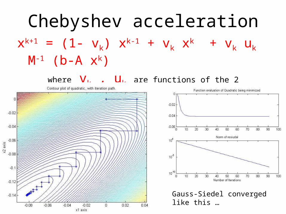
Chebyshev accelerationxk+1 = (1- vk) xk-1 + vk xk + vk uk M-1 (b-A xk)

where vk , uk are functions of the 2 extreme eigenvalues of G (not very expensive to get estimates of these eigenvalues)

Gauss-Siedel converged like this …

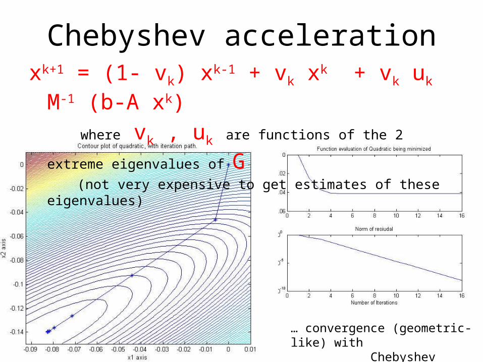
xk+1 = (1- vk) xk-1 + vk xk + vk uk M-1 (b-A xk)

where vk , uk are functions of the 2 extreme eigenvalues of G (not very expensive to get estimates of these eigenvalues)

… convergence (geometric-like) with Chebyshev acceleration

Chebyshev acceleration

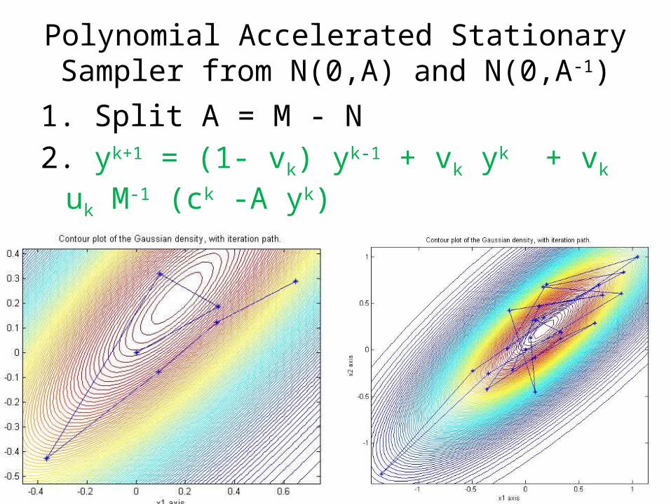
Polynomial Accelerated Stationary Sampler from N(0,A) and N(0,A-1)

1. Split A = M - N 2. yk+1 = (1- vk) yk-1 + vk yk + vk uk M-1 (ck -A yk) where ck ~ N(0, (2-vk)/vk ( (2 – uk)/ uk MT + N)

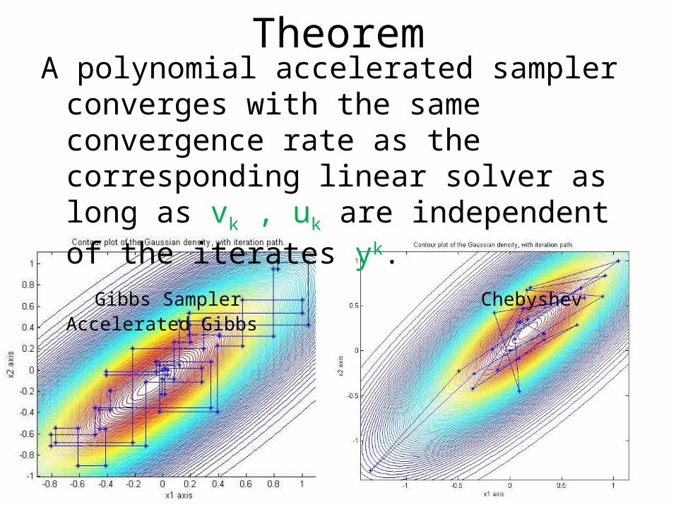
TheoremA polynomial accelerated sampler converges

with the same convergence rate as the corresponding linear solver as long as vk , uk are independent of the iterates yk.

Gibbs Sampler Chebyshev Accelerated Gibbs

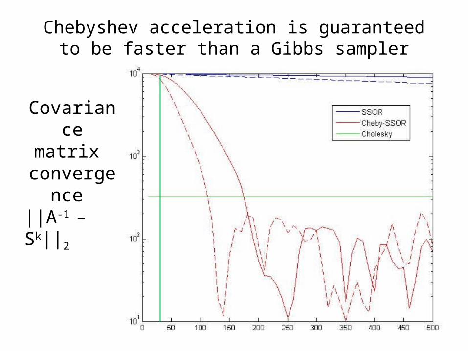
Chebyshev acceleration is guaranteed to be faster than a Gibbs sampler

Covariance matrix

convergence ||A-1 – Sk||2

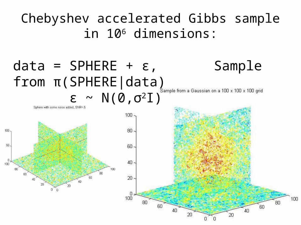
Chebyshev accelerated Gibbs samplein 106 dimensions:

data = SPHERE + ε, Sample from π(SPHERE|data) ε ~ N(0,σ2I)

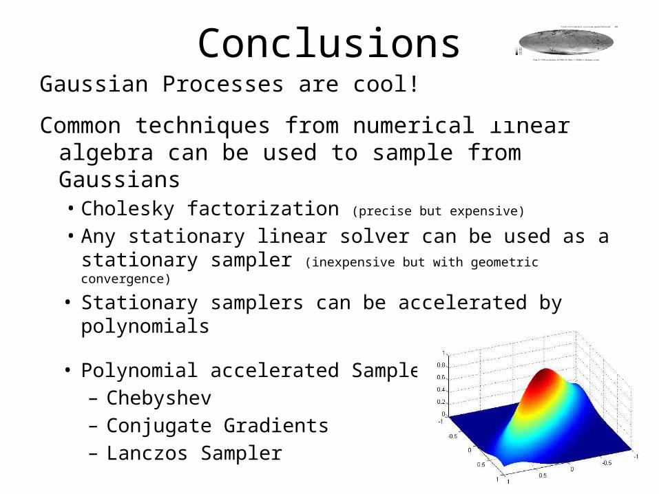
ConclusionsGaussian Processes are cool!

Common techniques from numerical linear algebra can be used to sample from Gaussians• Cholesky factorization (precise but expensive)

• Any stationary linear solver can be used as a stationary sampler (inexpensive but with geometric convergence)

• Stationary samplers can be accelerated by polynomials (guaranteed!)

• Polynomial accelerated Samplers– Chebyshev – Conjugate Gradients– Lanczos Sampler

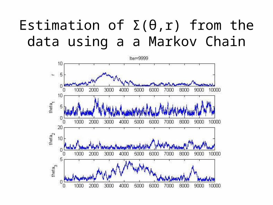
Estimation of Σ(θ,r) from the data using a a Markov Chain

Marginal Posteriors

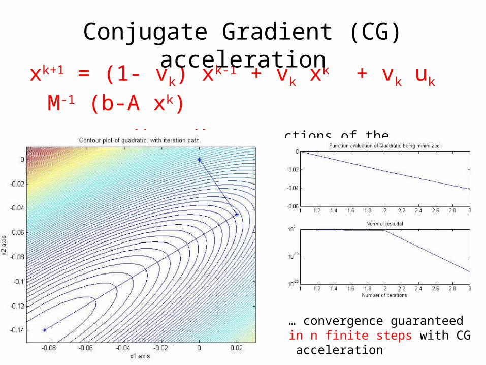
xk+1 = (1- vk) xk-1 + vk xk + vk uk M-1 (b-A xk)

where vk , uk are functions of the residuals b-Axk

… convergence guaranteed in n finite steps with CG acceleration

Conjugate Gradient (CG) acceleration

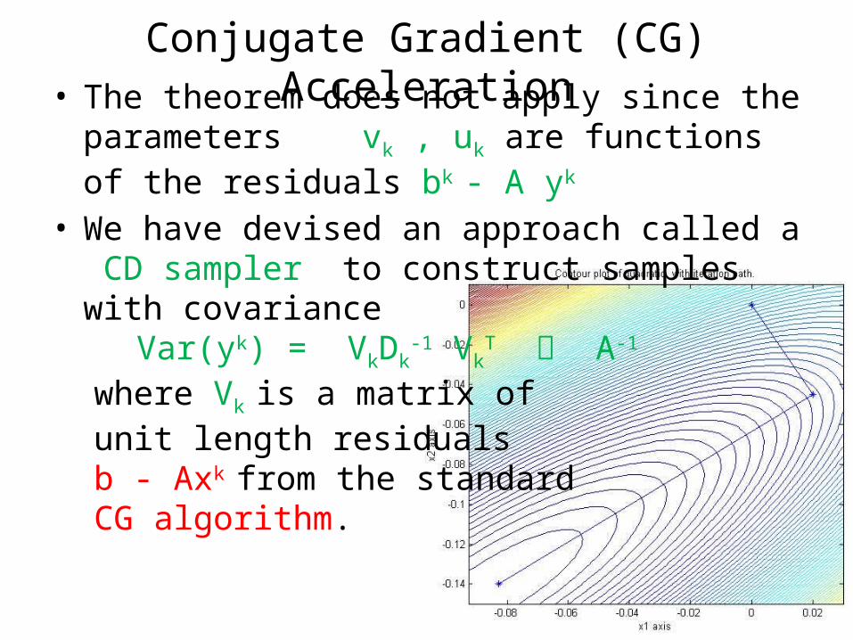
• The theorem does not apply since the parameters vk , uk are functions of the residuals bk - A yk

• We have devised an approach called a CD sampler to construct samples with covariance

Var(yk) = VkDk-1 Vk

T A-1

where Vk is a matrix of unit length residuals b - Axk from the standard CG algorithm.

Conjugate Gradient (CG) Acceleration

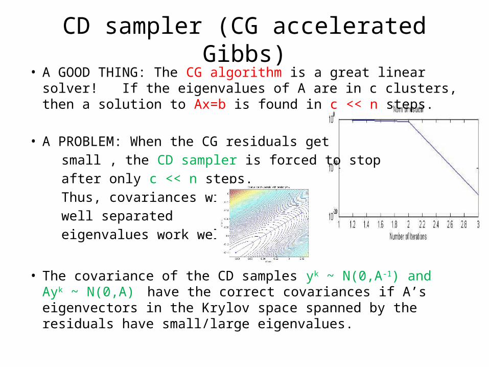
• A GOOD THING: The CG algorithm is a great linear solver! If the eigenvalues of A are in c clusters, then a solution to Ax=b is found in c << n steps.

• A PROBLEM: When the CG residuals get small , the CD sampler is forced to stop after only c << n steps. Thus, covariances with well separated eigenvalues work well.

• The covariance of the CD samples yk ~ N(0,A-1) and Ayk ~ N(0,A)

have the correct covariances if A’s eigenvectors in the Krylov space spanned by the residuals have small/large eigenvalues.

CD sampler (CG accelerated Gibbs)

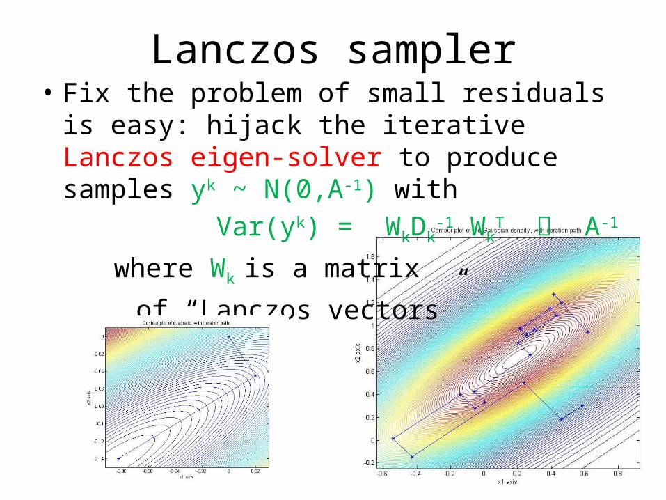
Lanczos sampler• Fix the problem of small residuals is easy:

hijack the iterative Lanczos eigen-solver to produce samples yk ~ N(0,A-1) with

Var(yk) = WkDk-1 Wk

T A-1

where Wk is a matrix

of “Lanczos vectors”

One extremely effective sampler for LARGE Gaussians

Use a combination of the ideas presented:• Generate samples with the CD or Lanczos

sampler while at the same time cheaply estimating the extreme eigenvalues of G.

• Seed these samples and extreme eigenvalues into a Chebyshev accelerated SOR sampler