Aggregate Loss ModelsChapter 9

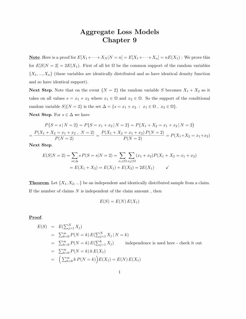
Note. Here is a proof for E[X1+· · ·+XN |N = n] = E[X1+· · ·+Xn] = nE(X1) : We prove this

for E[S|N = 2] = 2E(X1). First of all let Ω be the common support of the random variables

X1, ..., Xn (these variables are identically distributed and so have identical density function

and so have identical support).

Next Step. Note that on the event N = 2 the random variable S becomes X1 + X2 so it

takes on all values s = x1 + x2 where x1 ∈ Ω and x2 ∈ Ω. So the support of the conditional

random variable S|N = 2 is the set ∆ = s = x1 + x2 : x1 ∈ Ω , x2 ∈ Ω.

Next Step. For s ∈ ∆ we have

PS = s |N = 2 = PS = x1 + x2 |N = 2 = PX1 +X2 = x1 + x2 |N = 2

=P (X1 +X2 = x1 + x2 , N = 2)

P (N = 2)=

P (X1 +X2 = x1 + x2)P (N = 2)

P (N = 2)= P (X1+X2 = x1+x2)

Next Step.

E(S|N = 2) =∑s∈∆

s P (S = s|N = 2) =∑x1∈Ω

∑x2∈Ω

(x1 + x2)P (X1 +X2 = x1 + x2)

= E(X1 +X2) = E(X1) + E(X2) = 2E(X1)

Theorem. Let X1, X2, ... be an independent and identically distributed sample from a claim.

If the number of claims N is independent of the claim amount , then

E(S) = E(N)E(X1)

Proof.

E(S) = E(∑N

j=1Xj)

=∑∞

k=0 P (N = k)E(∑N

j=1Xj |N = k)

=∑∞

k=0 P (N = k)E(∑k

j=1Xj) independence is used here - check it out

=∑∞

k=0 P (N = k) k E(X1)

=(∑∞

k=0 k P (N = k))E(X1) = E(N)E(X1)

1

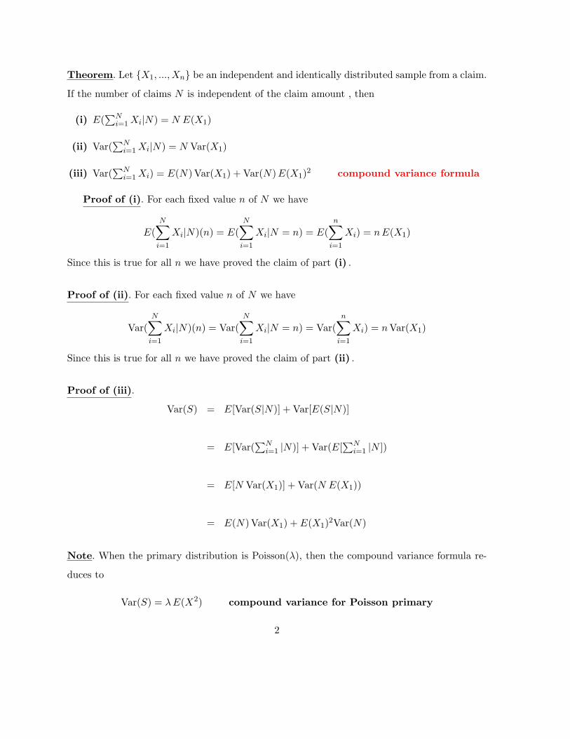
Theorem. Let X1, ..., Xn be an independent and identically distributed sample from a claim.

If the number of claims N is independent of the claim amount , then

(i) E(∑N

i=1Xi|N) = N E(X1)

(ii) Var(∑N

i=1Xi|N) = N Var(X1)

(iii) Var(∑N

i=1Xi) = E(N)Var(X1) + Var(N)E(X1)2 compound variance formula

Proof of (i). For each fixed value n of N we have

E(N∑i=1

Xi|N)(n) = E(N∑i=1

Xi|N = n) = E(n∑

i=1

Xi) = nE(X1)

Since this is true for all n we have proved the claim of part (i) .

Proof of (ii). For each fixed value n of N we have

Var(N∑i=1

Xi|N)(n) = Var(N∑i=1

Xi|N = n) = Var(n∑

i=1

Xi) = nVar(X1)

Since this is true for all n we have proved the claim of part (ii) .

Proof of (iii).

Var(S) = E[Var(S|N)] + Var[E(S|N)]

= E[Var(∑N

i=1 |N)] + Var(E[∑N

i=1 |N ])

= E[N Var(X1)] + Var(N E(X1))

= E(N)Var(X1) + E(X1)2Var(N)

Note. When the primary distribution is Poisson(λ), then the compound variance formula re-

duces to

Var(S) = λE(X2) compound variance for Poisson primary

2

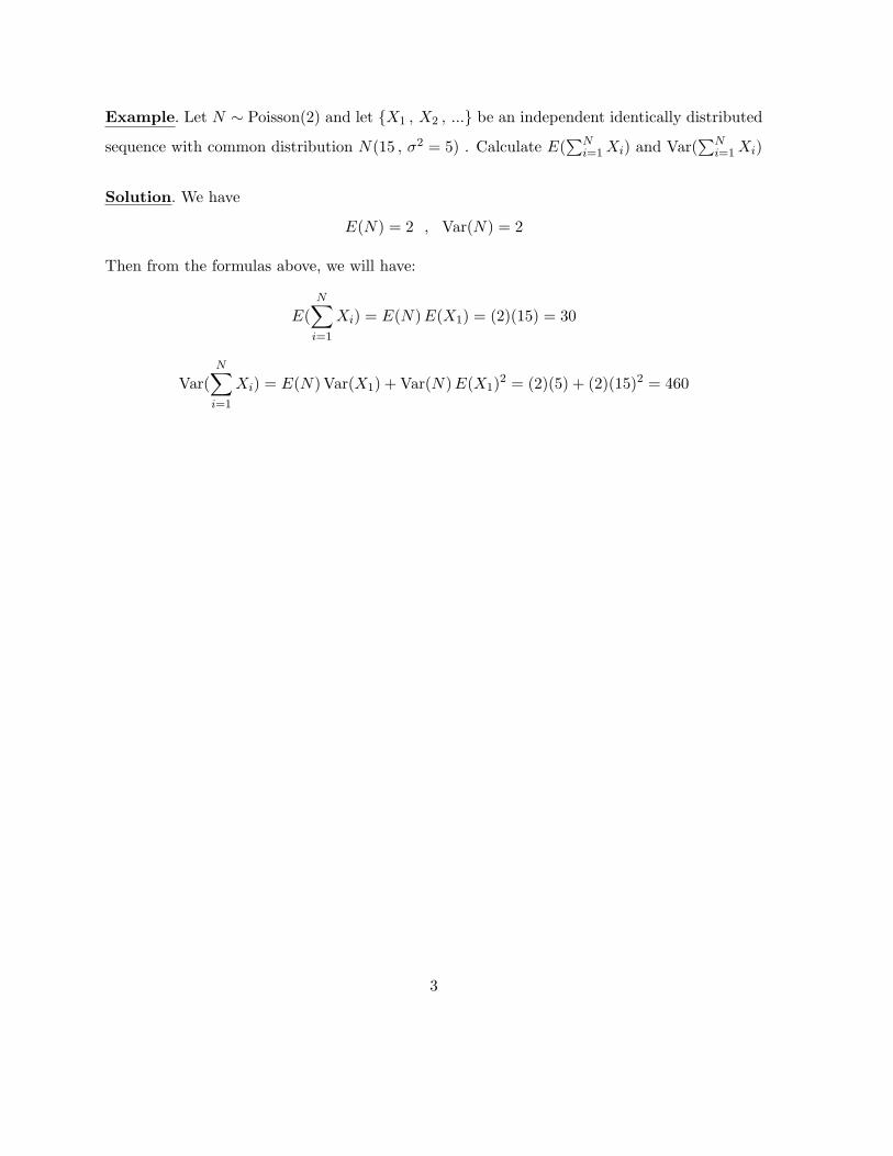
Example. Let N ∼ Poisson(2) and let X1 , X2 , ... be an independent identically distributed

sequence with common distribution N(15 , σ2 = 5) . Calculate E(∑N

i=1Xi) and Var(∑N

i=1Xi)

Solution. We have

E(N) = 2 , Var(N) = 2

Then from the formulas above, we will have:

E(N∑i=1

Xi) = E(N)E(X1) = (2)(15) = 30

Var(N∑i=1

Xi) = E(N)Var(X1) + Var(N)E(X1)2 = (2)(5) + (2)(15)2 = 460

3

Aggregate loss: total amount of loss in one period.

Individual risk model

Collective risk model

Individual risk model: is a model where we study the aggregate loss S = X1 + · · ·+Xn

where the losses X1, ..., Xn are (stochastically) independent.

Collective risk model: is a model where we study the aggregate loss S = X1 + · · ·+XN

where the losses X1, X2, ... are (stochastically) independent and identically distributed

(i.i.d.) and where N is a discrete random variable (called frequency) indicating the number

of losses, and that the Xi’s are independent of N . The distribution of N is called the

primary distribution and the common distribution of Xi’s is called the secondary

distribution. The collective model is a special case of compound distribution in which we

add up a random number of identically distributed random variables.

In an individual risk model, n is the number of insureds and Xi is the claim size for the

individual i. So under this model we can have P (Xi = 0) > 0 , i.e. there is positive chance

that the insured i will not have any claim in the period of study. But in the collective model,

N represents the variable number of claims and Xi denotes the i-th amount of the claim

that has occurred. So , under the collective model we have P (Xi = 0) = 0.

Convention: For N = 0 we set S = 0.

Example ∗. Let S have a Poisson frequency distribution with parameter λ = 5. The

individual claim amount has the following distribution:

x fX(x)

100 0.8

500 0.16

1000 0.04

Calculate the probability that aggregate claims will be exactly 600.

Solution.

Case 1. N = 2 in which we have

4

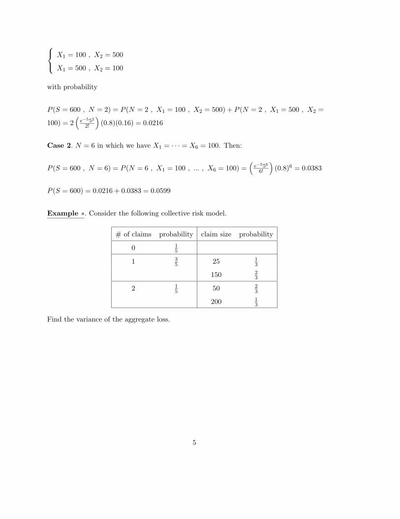
X1 = 100 , X2 = 500

X1 = 500 , X2 = 100

with probability

P (S = 600 , N = 2) = P (N = 2 , X1 = 100 , X2 = 500) + P (N = 2 , X1 = 500 , X2 =

100) = 2(e−552

2!

)(0.8)(0.16) = 0.0216

Case 2. N = 6 in which we have X1 = · · · = X6 = 100. Then:

P (S = 600 , N = 6) = P (N = 6 , X1 = 100 , ... , X6 = 100) =(e−556

6!

)(0.8)6 = 0.0383

P (S = 600) = 0.0216 + 0.0383 = 0.0599

Example ∗. Consider the following collective risk model.

# of claims probability claim size probability

0 15

1 35 25 1

3

150 23

2 15 50 2

3

200 13

Find the variance of the aggregate loss.

5

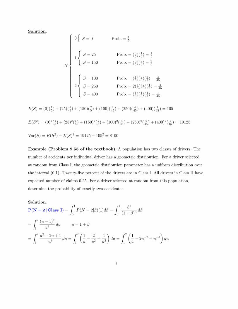
Solution.

N

0

S = 0 Prob. = 15

1

S = 25 Prob. = (35)(13) =

15

S = 150 Prob. = (35)(23) =

25

2

S = 100 Prob. = (15)(

23)(

23) =

445

S = 250 Prob. = 2(15)(23)(

13) =

445

S = 400 Prob. = (15)(13)(

13) =

145

E(S) = (0)(15) + (25)(15) + (150)(25) + (100)( 445) + (250)( 4

45) + (400)( 145) = 105

E(S2) = (0)2(15) + (25)2(15) + (150)2(25) + (100)2( 445) + (250)2( 4

45) + (400)2( 145) = 19125

Var(S) = E(S2)− E(S)2 = 19125− 1052 = 8100

Example (Problem 9.55 of the textbook). A population has two classes of drivers. The

number of accidents per individual driver has a geometric distribution. For a driver selected

at random from Class I, the geometric distribution parameter has a uniform distribution over

the interval (0,1). Twenty-five percent of the drivers are in Class I. All drivers in Class II have

expected number of claims 0.25. For a driver selected at random from this population,

determine the probability of exactly two accidents.

Solution.

P(N = 2 |Class I) =

∫ 1

0P (N = 2|β)(1)dβ =

∫ 1

0

β2

(1 + β)3dβ

=

∫ 2

1

(u− 1)2

u3du u = 1 + β

=

∫ 2

1

u2 − 2u+ 1

u3du =

∫ 2

1

(1

u− 2

u2+

1

u3

)du =

∫ 2

1

(1

u− 2u−2 + u−3

)du

6

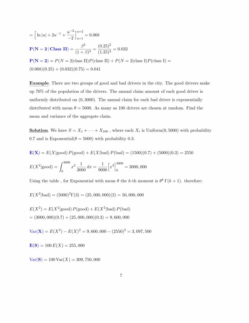
=[ln |u|+ 2u−1 +

u−2

−2

]u=2

u=1= 0.068

P(N = 2 |Class II) =β2

(1 + β)3=

(0.25)2

(1.25)3= 0.032

P(N = 2) = P (N = 2|class II)P (class II) + P (N = 2|class I)P (class I) =

(0.068)(0.25) + (0.032)(0.75) = 0.041

Example. There are two groups of good and bad drivers in the city. The good drivers make

up 70% of the population of the drivers. The annual claim amount of each good driver is

uniformly distributed on (0, 3000). The annual claim for each bad driver is exponentially

distributed with mean θ = 5000. As many as 100 drivers are chosen at random. Find the

mean and variance of the aggregate claim.

Solution. We have S = X1 + · · ·+X100 , where each Xi is Uniform(0, 5000) with probability

0.7 and is Exponential(θ = 5000) with probability 0.3.

E(X) = E(X|good)P (good) + E(X|bad)P (bad) = (1500)(0.7) + (5000)(0.3) = 2550

E(X2|good) =∫ 3000

0x2

1

3000dx =

1

9000

[x3

]30000

= 3000, 000

Using the table , for Exponential with mean θ the k-th moment is θk Γ(k + 1). therefore:

E(X2|bad) = (5000)2Γ(3) = (25, 000, 000)(2) = 50, 000, 000

E(X2) = E(X2|good)P (good) + E(X2|bad)P (bad)

= (3000, 000)(0.7) + (25, 000, 000)(0.3) = 9, 600, 000

Var(X) = E(X2)− E(X)2 = 9, 600, 000− (2550)2 = 3, 097, 500

E(S) = 100E(X) = 255, 000

Var(S) = 100Var(X) = 309, 750, 000

7

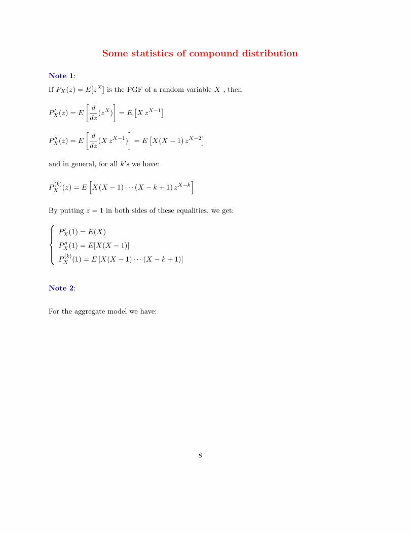
Some statistics of compound distribution

Note 1:

If PX(z) = E[zX ] is the PGF of a random variable X , then

P ′X(z) = E

[d

dz(zX)

]= E

[X zX−1

]P ′′X(z) = E

[d

dz(X zX−1)

]= E

[X(X − 1) zX−2

]and in general, for all k’s we have:

P(k)X (z) = E

[X(X − 1) · · · (X − k + 1) zX−k

]By putting z = 1 in both sides of these equalities, we get:

P ′X(1) = E(X)

P ′′X(1) = E[X(X − 1)]

P(k)X (1) = E [X(X − 1) · · · (X − k + 1)]

Note 2:

For the aggregate model we have:

8

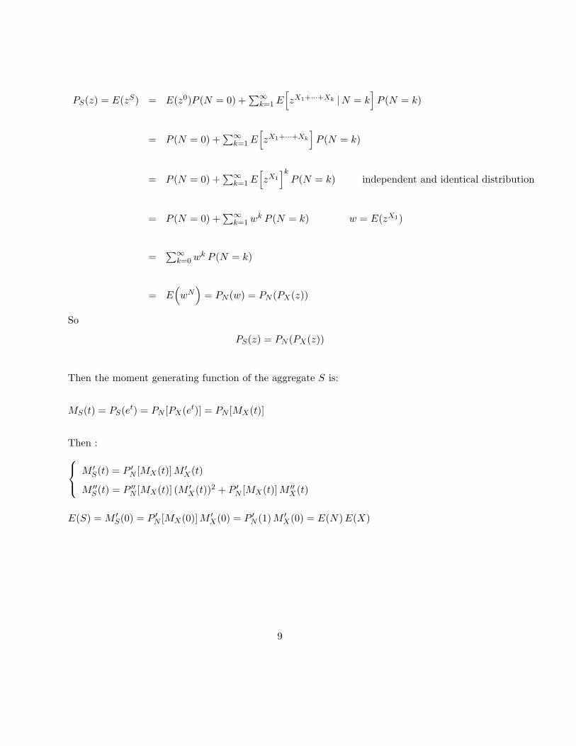
PS(z) = E(zS) = E(z0)P (N = 0) +∑∞

k=1E[zX1+···+Xk |N = k

]P (N = k)

= P (N = 0) +∑∞

k=1E[zX1+···+Xk

]P (N = k)

= P (N = 0) +∑∞

k=1E[zX1

]kP (N = k) independent and identical distribution

= P (N = 0) +∑∞

k=1wk P (N = k) w = E(zX1)

=∑∞

k=0wk P (N = k)

= E(wN

)= PN (w) = PN (PX(z))

So

PS(z) = PN (PX(z))

Then the moment generating function of the aggregate S is:

MS(t) = PS(et) = PN [PX(et)] = PN [MX(t)]

Then : M ′S(t) = P ′

N [MX(t)]M ′X(t)

M ′′S(t) = P ′′

N [MX(t)] (M ′X(t))2 + P ′

N [MX(t)]M ′′X(t)

E(S) = M ′S(0) = P ′

N [MX(0)]M ′X(0) = P ′

N (1)M ′X(0) = E(N)E(X)

9

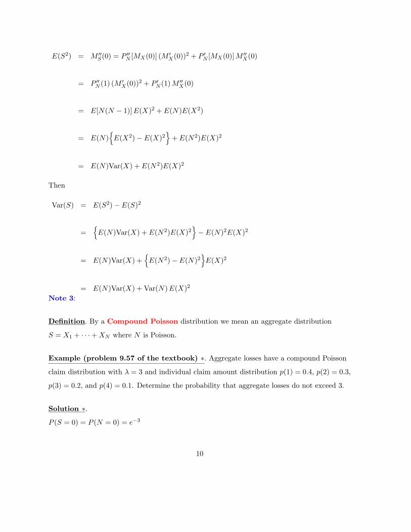
E(S2) = M ′′S(0) = P ′′

N [MX(0)] (M ′X(0))2 + P ′

N [MX(0)]M ′′X(0)

= P ′′N (1) (M ′

X(0))2 + P ′N (1)M ′′

X(0)

= E[N(N − 1)]E(X)2 + E(N)E(X2)

= E(N)E(X2)− E(X)2

+ E(N2)E(X)2

= E(N)Var(X) + E(N2)E(X)2

Then

Var(S) = E(S2)−E(S)2

=E(N)Var(X) + E(N2)E(X)2

− E(N)2E(X)2

= E(N)Var(X) +E(N2)− E(N)2

E(X)2

= E(N)Var(X) + Var(N)E(X)2

Note 3:

Definition. By a Compound Poisson distribution we mean an aggregate distribution

S = X1 + · · ·+XN where N is Poisson.

Example (problem 9.57 of the textbook) ∗. Aggregate losses have a compound Poisson

claim distribution with λ = 3 and individual claim amount distribution p(1) = 0.4, p(2) = 0.3,

p(3) = 0.2, and p(4) = 0.1. Determine the probability that aggregate losses do not exceed 3.

Solution ∗.

P (S = 0) = P (N = 0) = e−3

10

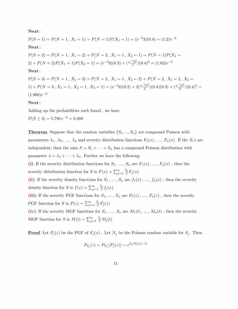
Next :

P (S = 1) = P (N = 1 , X1 = 1) = P (N = 1)P (X1 = 1) = (e−33)(0.4) = (1.2)e−3

Next :

P (S = 2) = P (N = 1 , X1 = 2) + P (N = 2 , X1 = 1 , X2 = 1) = P (N = 1)P (X1 =

2) + P (N = 2)P (X1 = 1)P (X2 = 1) = (e−33)(0.3) + ( e−332

2 )(0.4)2 = (1.62)e−3

Next :

P (S = 3) = P (N = 1 , X1 = 3) + P (N = 2 , X1 = 1 , X2 = 2) + P (N = 2 , X1 = 2 , X2 =

1) + P (N = 3 , X1 = 1 , X2 = 1 , X3 = 1) = (e−33)(0.2) + 2( e−332

2 )(0.4)(0.3) + ( e−333

3! )(0.4)3 =

(1.968)e−3

Next :

Adding up the probabilities such found , we have

P (S ≤ 3) = 5.788 e−3 = 0.288

Theorem. Suppose that the random variables S1, ..., Sn are compound Poisson with

parameters λ1 , λ2 , ... , λn and severity distribution functions F1(x) , ... , Fn(x). If the Si’s are

independent, then the sum S = S1 + · · ·+ Sn has a compound Poisson distribution with

parameter λ = λ1 + · · ·+ λn. Further we have the following:

(i): If the severity distribution functions for S1 , ... , Sn are F1(x) , ... , Fn(x) , then the

severity distribution function for S is F (x) =∑n

j=1λj

λ Fj(x)

(ii): If the severity density functions for S1 , ... , Sn are f1(x) , ... , fn(x) , then the severity

density function for S is f(x) =∑n

j=1λj

λ fj(x)

(iii): If the severity PGF functions for S1 , ... , Sn are P1(z) , ... , Pn(z) , then the severity

PGF function for S is P (z) =∑n

j=1λj

λ Pj(z)

(iv): If the severity MGF functions for S1 , ... , Sn are M1(t) , ... , Mn(t) , then the severity

MGF function for S is M(t) =∑n

j=1λj

λ Mj(t)

Proof. Let Pj(z) be the PGF of Fj(x) . Let Nj be the Poisson random variable for Sj . Then

PSj (z) = PNj (Pj(z)) = eλj(Pj(z)−1)

11

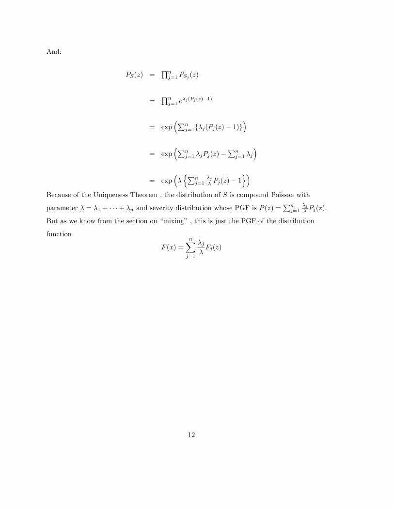
And:

PS(z) =∏n

j=1 PSj (z)

=∏n

j=1 eλj(Pj(z)−1)

= exp(∑n

j=1λj(Pj(z)− 1))

= exp(∑n

j=1 λjPj(z)−∑n

j=1 λj

)

= exp(λ∑n

j=1λj

λ Pj(z)− 1)

Because of the Uniqueness Theorem , the distribution of S is compound Poisson with

parameter λ = λ1 + · · ·+ λn and severity distribution whose PGF is P (z) =∑n

j=1λj

λ Pj(z).

But as we know from the section on “mixing” , this is just the PGF of the distribution

function

F (x) =

n∑j=1

λj

λFj(z)

12

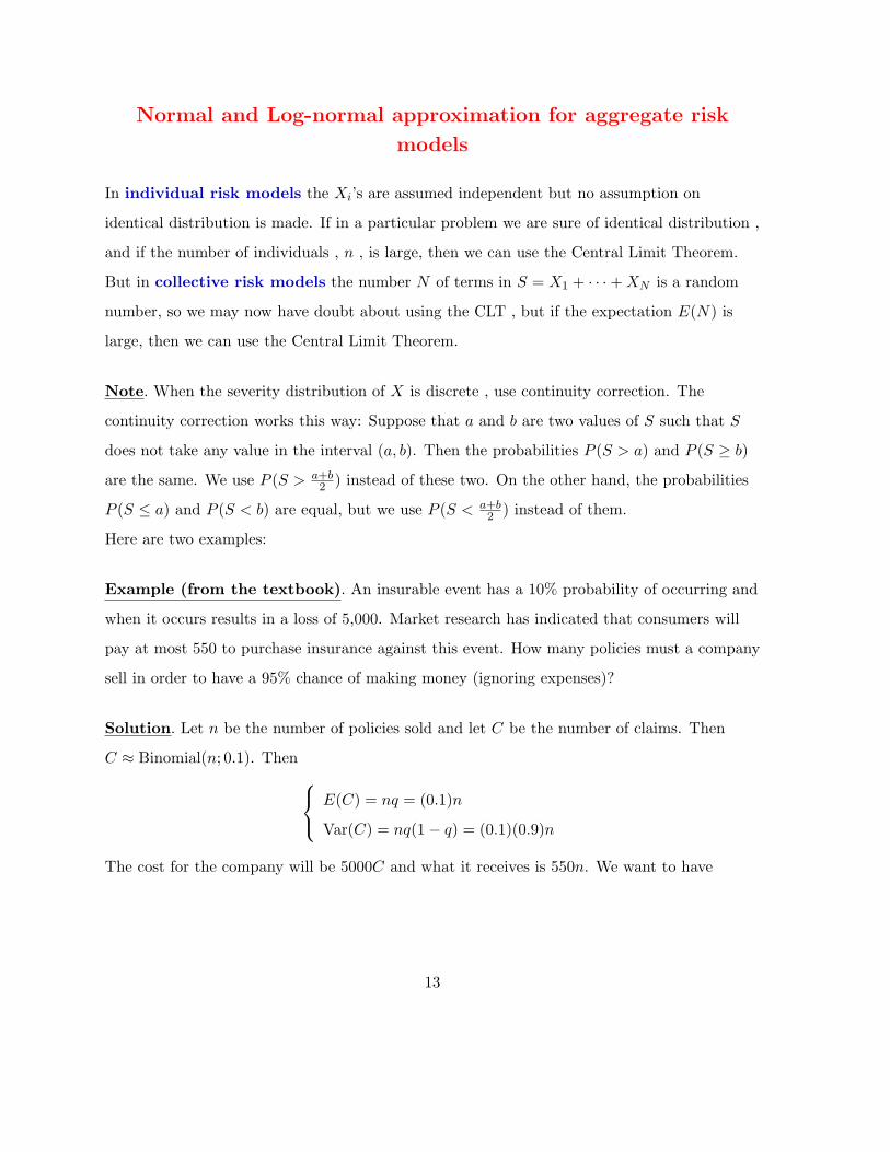
Normal and Log-normal approximation for aggregate risk

models

In individual risk models the Xi’s are assumed independent but no assumption on

identical distribution is made. If in a particular problem we are sure of identical distribution ,

and if the number of individuals , n , is large, then we can use the Central Limit Theorem.

But in collective risk models the number N of terms in S = X1 + · · ·+XN is a random

number, so we may now have doubt about using the CLT , but if the expectation E(N) is

large, then we can use the Central Limit Theorem.

Note. When the severity distribution of X is discrete , use continuity correction. The

continuity correction works this way: Suppose that a and b are two values of S such that S

does not take any value in the interval (a, b). Then the probabilities P (S > a) and P (S ≥ b)

are the same. We use P (S > a+b2 ) instead of these two. On the other hand, the probabilities

P (S ≤ a) and P (S < b) are equal, but we use P (S < a+b2 ) instead of them.

Here are two examples:

Example (from the textbook). An insurable event has a 10% probability of occurring and

when it occurs results in a loss of 5,000. Market research has indicated that consumers will

pay at most 550 to purchase insurance against this event. How many policies must a company

sell in order to have a 95% chance of making money (ignoring expenses)?

Solution. Let n be the number of policies sold and let C be the number of claims. Then

C ≈ Binomial(n; 0.1). Then E(C) = nq = (0.1)n

Var(C) = nq(1− q) = (0.1)(0.9)n

The cost for the company will be 5000C and what it receives is 550n. We want to have

13

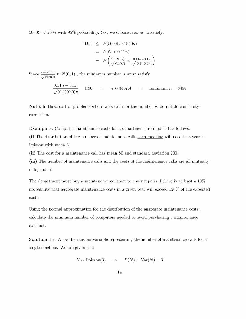
5000C < 550n with 95% probability. So , we choose n so as to satisfy:

0.95 ≤ P (5000C < 550n)

= P (C < 0.11n)

= P

(C−E(C)√Var(C)

< 0.11n−0.1n√(0.1)(0.9)n

)Since C−E(C)√

Var(C)≈ N(0, 1) , the minimum number n must satisfy

0.11n− 0.1n√(0.1)(0.9)n

= 1.96 ⇒ n ≈ 3457.4 ⇒ minimum n = 3458

Note. In these sort of problems where we search for the number n, do not do continuity

correction.

Example ∗. Computer maintenance costs for a department are modeled as follows:

(i) The distribution of the number of maintenance calls each machine will need in a year is

Poisson with mean 3.

(ii) The cost for a maintenance call has mean 80 and standard deviation 200.

(iii) The number of maintenance calls and the costs of the maintenance calls are all mutually

independent.

The department must buy a maintenance contract to cover repairs if there is at least a 10%

probability that aggregate maintenance costs in a given year will exceed 120% of the expected

costs.

Using the normal approximation for the distribution of the aggregate maintenance costs,

calculate the minimum number of computers needed to avoid purchasing a maintenance

contract.

Solution. Let N be the random variable representing the number of maintenance calls for a

single machine. We are given that

N ∼ Poisson(3) ⇒ E(N) = Var(N) = 3

14

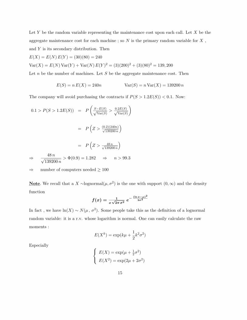
Let Y be the random variable representing the maintenance cost upon each call. Let X be the

aggregate maintenance cost for each machine ; so N is the primary random variable for X ,

and Y is its secondary distribution. Then

E(X) = E(N)E(Y ) = (30)(80) = 240

Var(X) = E(N)Var(Y ) + Var(N)E(Y )2 = (3)(200)2 + (3)(80)2 = 139, 200

Let n be the number of machines. Let S be the aggregate maintenance cost. Then

E(S) = nE(X) = 240n Var(S) = nVar(X) = 139200n

The company will avoid purchasing the contracts if P (S > 1.2E(S)) < 0.1. Now:

0.1 > P (S > 1.2E(S)) = P

(S−E(S)√Var(S)

> 0.2E(S)√Var(S)

)

= P(Z > (0.2)(240n)√

139200n

)

= P(Z > 48n√

139200n

)⇒ 48n√

139200n> Φ(0.9) = 1.282 ⇒ n > 99.3

⇒ number of computers needed ≥ 100

Note. We recall that a X ∼lognormal(µ, σ2) is the one with support (0,∞) and the density

function

f(x) = 1

x√

2π σ2e−

(ln x−µ)2

2σ2

In fact , we have ln(X) ∼ N(µ , σ2). Some people take this as the definition of a lognormal

random variable: it is a r.v. whose logarithm is normal. One can easily calculate the raw

moments :

E(Xk) = exp(kµ+1

2k2σ2)

Especially E(X) = exp(µ+ 12σ

2)

E(X2) = exp(2µ+ 2σ2)

15

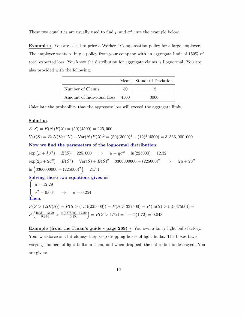
These two equalities are usually used to find µ and σ2 ; see the example below.

Example ∗. You are asked to price a Workers’ Compensation policy for a large employer.

The employer wants to buy a policy from your company with an aggregate limit of 150% of

total expected loss. You know the distribution for aggregate claims is Lognormal. You are

also provided with the following:

Mean Standard Deviation

Number of Claims 50 12

Amount of Individual Loss 4500 3000

Calculate the probability that the aggregate loss will exceed the aggregate limit.

Solution.

E(S) = E(N)E(X) = (50)(4500) = 225, 000

Var(S) = E(N)Var(X) + Var(N)E(X)2 = (50)(3000)2 + (12)2(4500) = 3, 366, 000, 000

Now we find the parameters of the lognormal distribution:

exp(µ+ 1

2σ2)= E(S) = 225, 000 ⇒ µ+ 1

2σ2 = ln(225000) = 12.32

exp(2µ+ 2σ2) = E(S2) = Var(S) + E(S)2 = 3366000000 + (225000)2 ⇒ 2µ+ 2σ2 =

ln(3366000000 + (225000)2

)= 24.71

Solving these two equations gives us: µ = 12.29

σ2 = 0.064 ⇒ σ = 0.254

Then:

P (S > 1.5E(S)) = P (S > (1.5)(225000)) = P (S > 337500) = P (ln(S) > ln(337500)) =

P(ln(S)−12.29

0.254 > ln(337500)−12.290.254

)= P (Z > 1.72) = 1− Φ(1.72) = 0.043

Example (from the Finan’s guide - page 269) ∗. You own a fancy light bulb factory.

Your workforce is a bit clumsy they keep dropping boxes of light bulbs. The boxes have

varying numbers of light bulbs in them, and when dropped, the entire box is destroyed. You

are given:

16

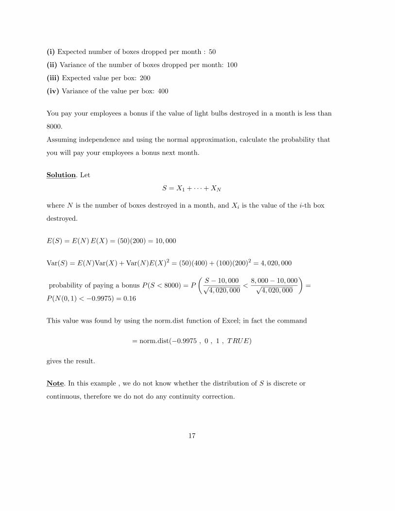
(i) Expected number of boxes dropped per month : 50

(ii) Variance of the number of boxes dropped per month: 100

(iii) Expected value per box: 200

(iv) Variance of the value per box: 400

You pay your employees a bonus if the value of light bulbs destroyed in a month is less than

8000.

Assuming independence and using the normal approximation, calculate the probability that

you will pay your employees a bonus next month.

Solution. Let

S = X1 + · · ·+XN

where N is the number of boxes destroyed in a month, and Xi is the value of the i-th box

destroyed.

E(S) = E(N)E(X) = (50)(200) = 10, 000

Var(S) = E(N)Var(X) + Var(N)E(X)2 = (50)(400) + (100)(200)2 = 4, 020, 000

probability of paying a bonus P (S < 8000) = P

(S − 10, 000√4, 020, 000

<8, 000− 10, 000√

4, 020, 000

)=

P (N(0, 1) < −0.9975) = 0.16

This value was found by using the norm.dist function of Excel; in fact the command

= norm.dist(−0.9975 , 0 , 1 , TRUE)

gives the result.

Note. In this example , we do not know whether the distribution of S is discrete or

continuous, therefore we do not do any continuity correction.

17

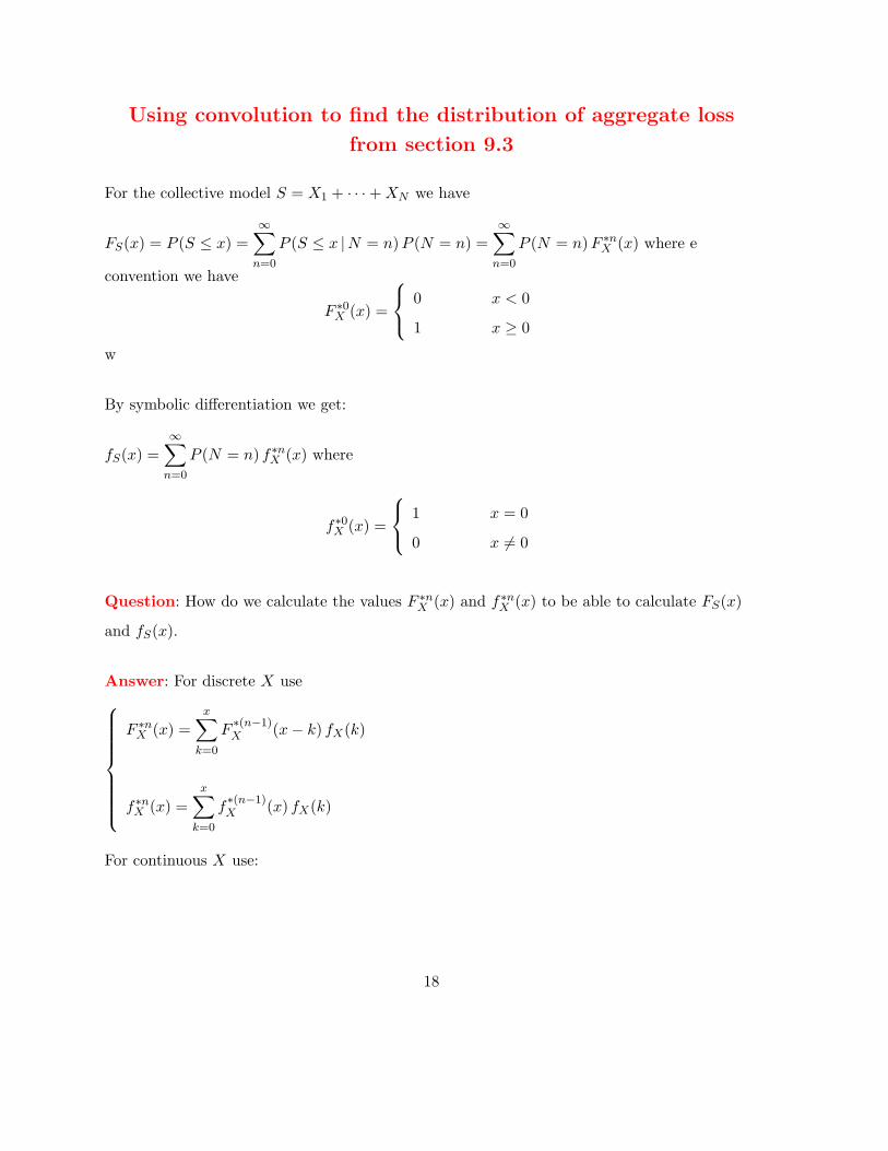
Using convolution to find the distribution of aggregate loss

from section 9.3

For the collective model S = X1 + · · ·+XN we have

FS(x) = P (S ≤ x) =

∞∑n=0

P (S ≤ x |N = n)P (N = n) =

∞∑n=0

P (N = n)F ∗nX (x) where e

convention we have

F ∗0X (x) =

0 x < 0

1 x ≥ 0

w

By symbolic differentiation we get:

fS(x) =∞∑n=0

P (N = n) f∗nX (x) where

f∗0X (x) =

1 x = 0

0 x = 0

Question: How do we calculate the values F ∗nX (x) and f∗n

X (x) to be able to calculate FS(x)

and fS(x).

Answer: For discrete X use

F ∗nX (x) =

x∑k=0

F∗(n−1)X (x− k) fX(k)

f∗nX (x) =

x∑k=0

f∗(n−1)X (x) fX(k)

For continuous X use:

18

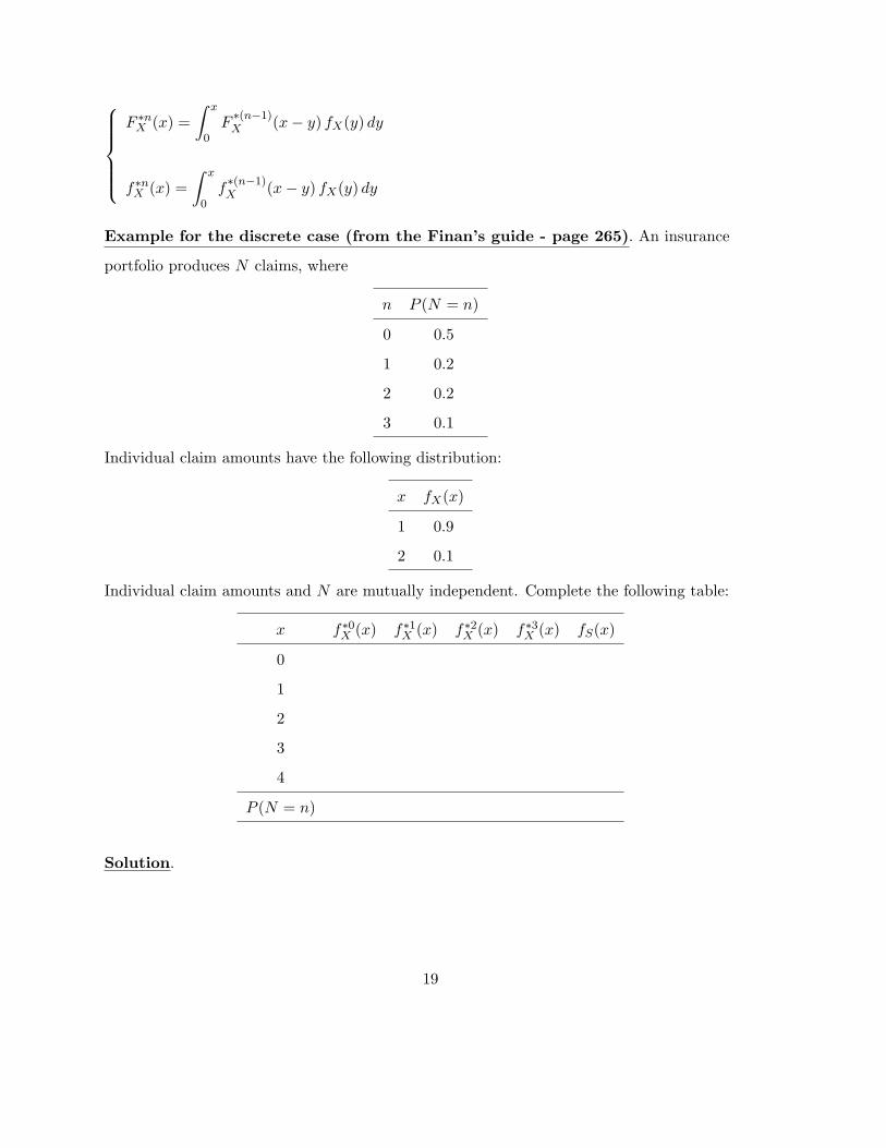
F ∗nX (x) =

∫ x

0F

∗(n−1)X (x− y) fX(y) dy

f∗nX (x) =

∫ x

0f∗(n−1)X (x− y) fX(y) dy

Example for the discrete case (from the Finan’s guide - page 265). An insurance

portfolio produces N claims, where

n P (N = n)

0 0.5

1 0.2

2 0.2

3 0.1

Individual claim amounts have the following distribution:

x fX(x)

1 0.9

2 0.1

Individual claim amounts and N are mutually independent. Complete the following table:

x f∗0X (x) f∗1

X (x) f∗2X (x) f∗3

X (x) fS(x)

0

1

2

3

4

P (N = n)

Solution.

19

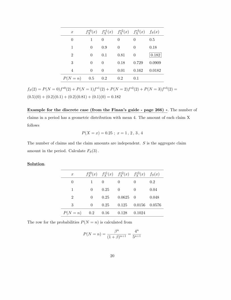
x f∗0X (x) f∗1

X (x) f∗2X (x) f∗3

X (x) fS(x)

0 1 0 0 0 0.5

1 0 0.9 0 0 0.18

2 0 0.1 0.81 0 0.182

3 0 0 0.18 0.729 0.0909

4 0 0 0.01 0.162 0.0182

P (N = n) 0.5 0.2 0.2 0.1

fS(2) = P (N = 0)f∗0(2) + P (N = 1)f∗1(2) + P (N = 2)f∗2(2) + P (N = 3)f∗3(2) =

(0.5)(0) + (0.2)(0.1) + (0.2)(0.81) + (0.1)(0) = 0.182

Example for the discrete case (from the Finan’s guide - page 266) ∗. The number of

claims in a period has a geometric distribution with mean 4. The amount of each claim X

follows

P (X = x) = 0.25 ; x = 1 , 2 , 3 , 4

The number of claims and the claim amounts are independent. S is the aggregate claim

amount in the period. Calculate FS(3) .

Solution.

x f∗0X (x) f∗1

X (x) f∗2X (x) f∗3

X (x) fS(x)

0 1 0 0 0 0.2

1 0 0.25 0 0 0.04

2 0 0.25 0.0625 0 0.048

3 0 0.25 0.125 0.0156 0.0576

P (N = n) 0.2 0.16 0.128 0.1024

The row for the probabilities P (N = n) is calculated from

P (N = n) =βn

(1 + β)n+1=

4n

5n+1

20

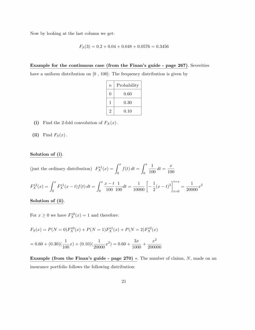
Now by looking at the last column we get:

FS(3) = 0.2 + 0.04 + 0.048 + 0.0576 = 0.3456

Example for the continuous case (from the Finan’s guide - page 267). Severities

have a uniform distribution on [0 , 100]: The frequency distribution is given by

n Probability

0 0.60

1 0.30

2 0.10

(i) Find the 2-fold convolution of FX(x) .

(ii) Find FS(x) .

Solution of (i).

(just the ordinary distribution) F ∗1X (x) =

∫ x

0f(t) dt =

∫ x

0

1

100dt =

x

100

F ∗2X (x) =

∫ x

0F ∗1X (x− t)f(t) dt =

∫ x

0

x− t

100

1

100dt =

1

10000

[− 1

2(x− t)2

]t=x

t=0

=1

20000x2

Solution of (ii).

For x ≥ 0 we have F ∗0X (x) = 1 and therefore:

FS(x) = P (N = 0)F ∗0X (x) + P (N = 1)F ∗1

X (x) + P (N = 2)F ∗2X (x)

= 0.60 + (0.30)(1

100x) + (0.10)(

1

20000x2) = 0.60 +

3x

1000+

x2

200000

Example (from the Finan’s guide - page 270) ∗. The number of claims, N , made on an

insurance portfolio follows the following distribution:

21

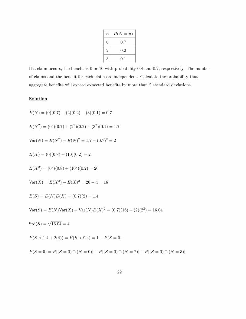
n P (N = n)

0 0.7

2 0.2

3 0.1

If a claim occurs, the benefit is 0 or 10 with probability 0.8 and 0.2, respectively. The number

of claims and the benefit for each claim are independent. Calculate the probability that

aggregate benefits will exceed expected benefits by more than 2 standard deviations.

Solution.

E(N) = (0)(0.7) + (2)(0.2) + (3)(0.1) = 0.7

E(N2) = (02)(0.7) + (22)(0.2) + (32)(0.1) = 1.7

Var(N) = E(N2)− E(N)2 = 1.7− (0.7)2 = 2

E(X) = (0)(0.8) + (10)(0.2) = 2

E(X2) = (02)(0.8) + (102)(0.2) = 20

Var(X) = E(X2)− E(X)2 = 20− 4 = 16

E(S) = E(N)E(X) = (0.7)(2) = 1.4

Var(S) = E(N)Var(X) + Var(N)E(X)2 = (0.7)(16) + (2)(22) = 16.04

Std(S) =√16.04 = 4

P (S > 1.4 + 2(4)) = P (S > 9.4) = 1− P (S = 0)

P (S = 0) = P [(S = 0) ∩ (N = 0)] + P [(S = 0) ∩ (N = 2)] + P [(S = 0) ∩ (N = 3)]

22

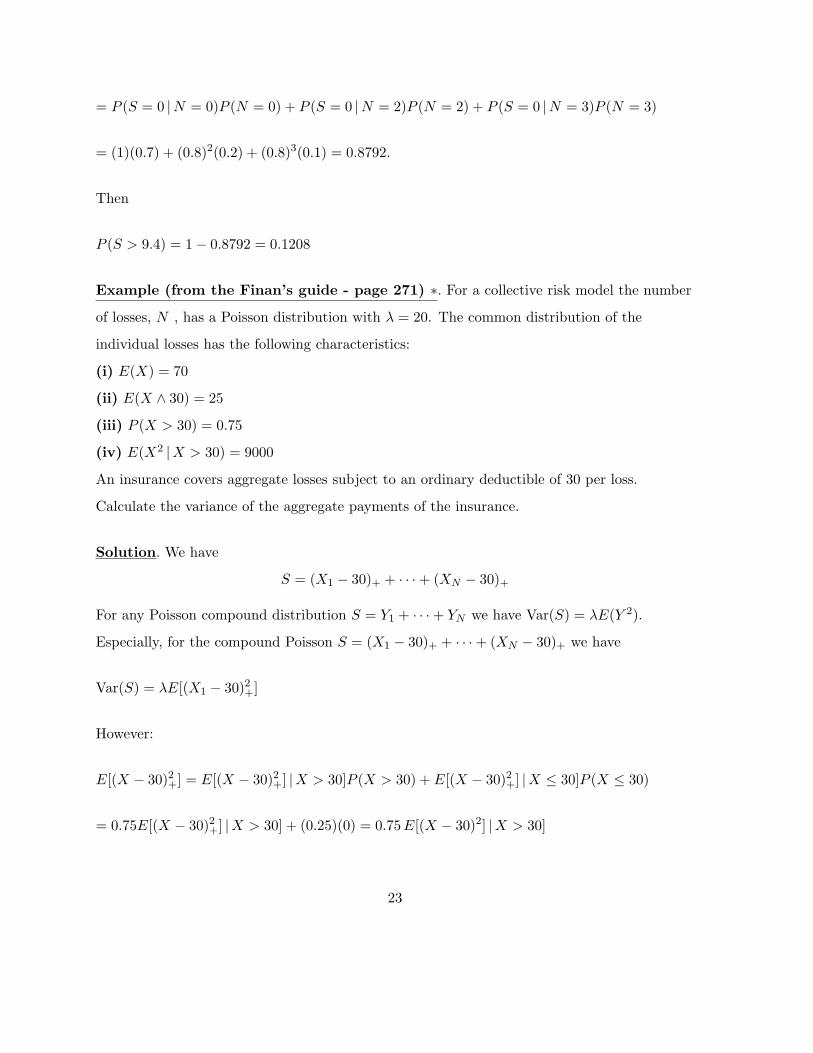
= P (S = 0 |N = 0)P (N = 0) + P (S = 0 |N = 2)P (N = 2) + P (S = 0 |N = 3)P (N = 3)

= (1)(0.7) + (0.8)2(0.2) + (0.8)3(0.1) = 0.8792.

Then

P (S > 9.4) = 1− 0.8792 = 0.1208

Example (from the Finan’s guide - page 271) ∗. For a collective risk model the number

of losses, N , has a Poisson distribution with λ = 20. The common distribution of the

individual losses has the following characteristics:

(i) E(X) = 70

(ii) E(X ∧ 30) = 25

(iii) P (X > 30) = 0.75

(iv) E(X2 |X > 30) = 9000

An insurance covers aggregate losses subject to an ordinary deductible of 30 per loss.

Calculate the variance of the aggregate payments of the insurance.

Solution. We have

S = (X1 − 30)+ + · · ·+ (XN − 30)+

For any Poisson compound distribution S = Y1 + · · ·+ YN we have Var(S) = λE(Y 2).

Especially, for the compound Poisson S = (X1 − 30)+ + · · ·+ (XN − 30)+ we have

Var(S) = λE[(X1 − 30)2+]

However:

E[(X − 30)2+] = E[(X − 30)2+] |X > 30]P (X > 30) + E[(X − 30)2+] |X ≤ 30]P (X ≤ 30)

= 0.75E[(X − 30)2+] |X > 30] + (0.25)(0) = 0.75E[(X − 30)2] |X > 30]

23

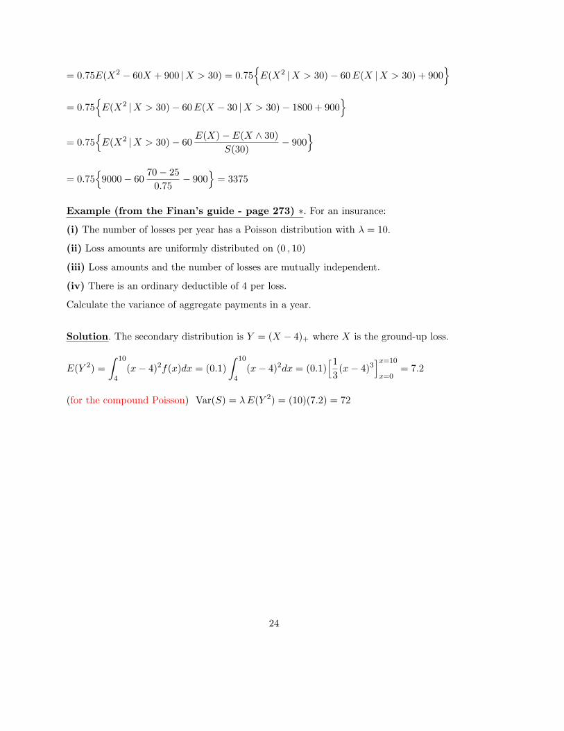
= 0.75E(X2 − 60X + 900 |X > 30) = 0.75E(X2 |X > 30)− 60E(X |X > 30) + 900

= 0.75

E(X2 |X > 30)− 60E(X − 30 |X > 30)− 1800 + 900

= 0.75

E(X2 |X > 30)− 60

E(X)− E(X ∧ 30)

S(30)− 900

= 0.759000− 60

70− 25

0.75− 900

= 3375

Example (from the Finan’s guide - page 273) ∗. For an insurance:

(i) The number of losses per year has a Poisson distribution with λ = 10.

(ii) Loss amounts are uniformly distributed on (0 , 10)

(iii) Loss amounts and the number of losses are mutually independent.

(iv) There is an ordinary deductible of 4 per loss.

Calculate the variance of aggregate payments in a year.

Solution. The secondary distribution is Y = (X − 4)+ where X is the ground-up loss.

E(Y 2) =

∫ 10

4(x− 4)2f(x)dx = (0.1)

∫ 10

4(x− 4)2dx = (0.1)

[13(x− 4)3

]x=10

x=0= 7.2

(for the compound Poisson) Var(S) = λE(Y 2) = (10)(7.2) = 72

24

Stop Loss Insurance

from section 9.3

When a deductible d is applied to the aggregate loss S , the resulting payment

(S − d)+ =

0 S ≤ d

S − d S > d

is called stop-loss insurance. The expected value E[(S − d)+] is called net stop-loss

premium. As usual, we have

E[(S − d)+] =

∫∞d [1− FS(x)]dx =

∫∞d (x− d)fS(x) dx

∑x>d[1− FS(x)] =

∑x>d(x− d)fS(x)

Note. Although this equality is true in theory, but it is not so practical to use it because it is

difficult to determine the support of the random variable S and so we might not know the

upper limit of this integration (analyse this difficulty for the next example). A practical way

of using this premium is to use the equality

E[(S − d)+] = E(S)− E(S ∧ d) = E(N)E(X)− E(S ∧ d)

Example. Severities have a uniform distribution on [0 , 100]: The frequency distribution is

given by

n Probability

0 0.60

1 0.30

2 0.10

Calculate E[(S − 5)+].

Solution.

25

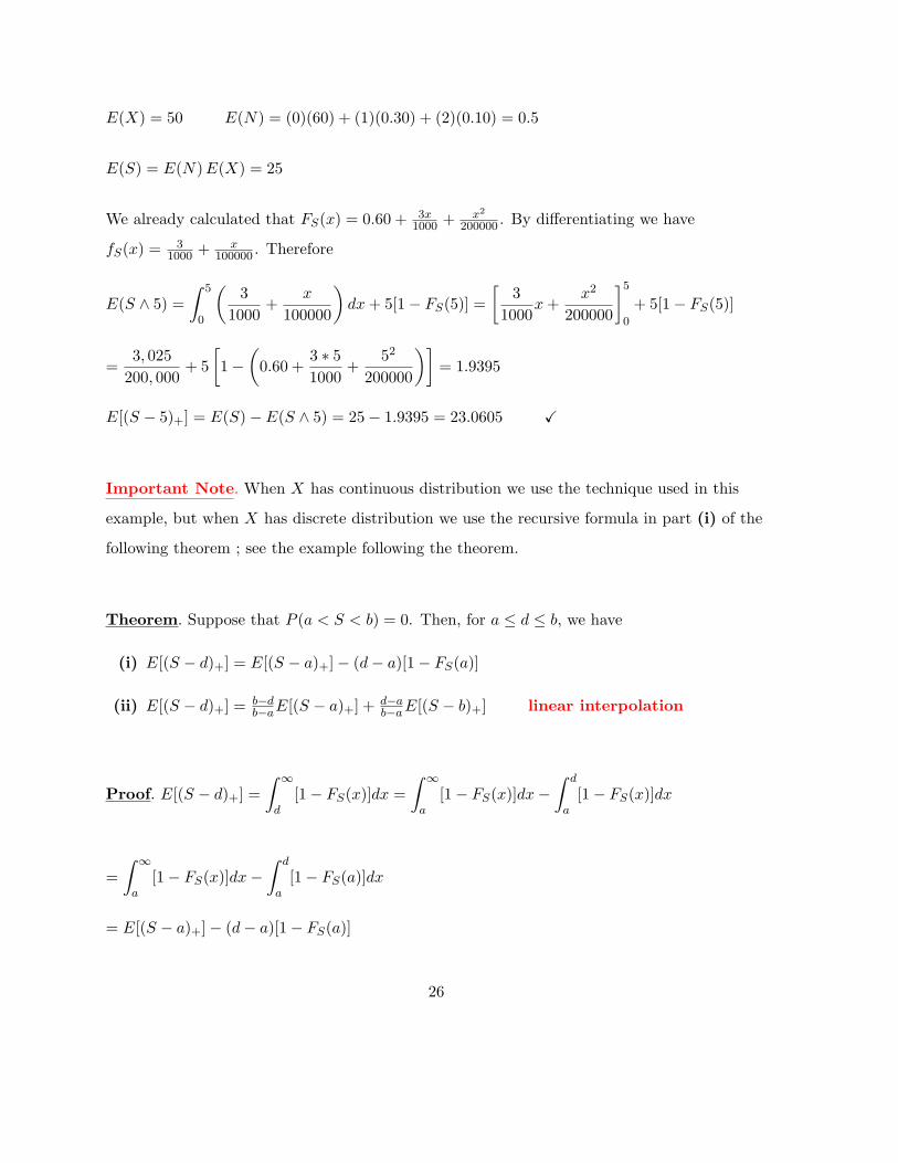
E(X) = 50 E(N) = (0)(60) + (1)(0.30) + (2)(0.10) = 0.5

E(S) = E(N)E(X) = 25

We already calculated that FS(x) = 0.60 + 3x1000 + x2

200000 . By differentiating we have

fS(x) =3

1000 + x100000 . Therefore

E(S ∧ 5) =

∫ 5

0

(3

1000+

x

100000

)dx+ 5[1− FS(5)] =

[3

1000x+

x2

200000

]50

+ 5[1− FS(5)]

=3, 025

200, 000+ 5

[1−

(0.60 +

3 ∗ 51000

+52

200000

)]= 1.9395

E[(S − 5)+] = E(S)− E(S ∧ 5) = 25− 1.9395 = 23.0605

Important Note. When X has continuous distribution we use the technique used in this

example, but when X has discrete distribution we use the recursive formula in part (i) of the

following theorem ; see the example following the theorem.

Theorem. Suppose that P (a < S < b) = 0. Then, for a ≤ d ≤ b, we have

(i) E[(S − d)+] = E[(S − a)+]− (d− a)[1− FS(a)]

(ii) E[(S − d)+] =b−db−aE[(S − a)+] +

d−ab−aE[(S − b)+] linear interpolation

Proof. E[(S − d)+] =

∫ ∞

d[1− FS(x)]dx =

∫ ∞

a[1− FS(x)]dx−

∫ d

a[1− FS(x)]dx

=

∫ ∞

a[1− FS(x)]dx−

∫ d

a[1− FS(a)]dx

= E[(S − a)+]− (d− a)[1− FS(a)]

26

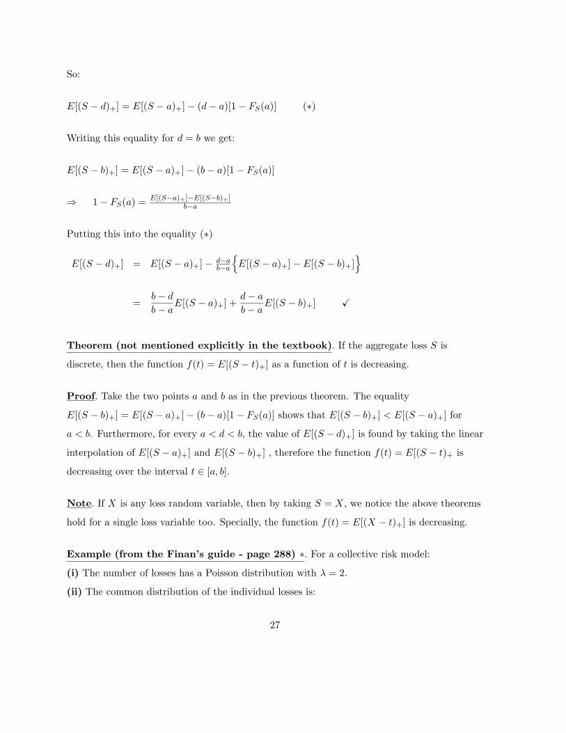
So:

E[(S − d)+] = E[(S − a)+]− (d− a)[1− FS(a)] (∗)

Writing this equality for d = b we get:

E[(S − b)+] = E[(S − a)+]− (b− a)[1− FS(a)]

⇒ 1− FS(a) =E[(S−a)+]−E[(S−b)+]

b−a

Putting this into the equality (∗)

E[(S − d)+] = E[(S − a)+]− d−ab−a

E[(S − a)+]−E[(S − b)+]

=b− d

b− aE[(S − a)+] +

d− a

b− aE[(S − b)+]

Theorem (not mentioned explicitly in the textbook). If the aggregate loss S is

discrete, then the function f(t) = E[(S − t)+] as a function of t is decreasing.

Proof. Take the two points a and b as in the previous theorem. The equality

E[(S − b)+] = E[(S − a)+]− (b− a)[1− FS(a)] shows that E[(S − b)+] < E[(S − a)+] for

a < b. Furthermore, for every a < d < b, the value of E[(S − d)+] is found by taking the linear

interpolation of E[(S − a)+] and E[(S − b)+] , therefore the function f(t) = E[(S − t)+ is

decreasing over the interval t ∈ [a, b].

Note. If X is any loss random variable, then by taking S = X, we notice the above theorems

hold for a single loss variable too. Specially, the function f(t) = E[(X − t)+] is decreasing.

Example (from the Finan’s guide - page 288) ∗. For a collective risk model:

(i) The number of losses has a Poisson distribution with λ = 2.

(ii) The common distribution of the individual losses is:

27

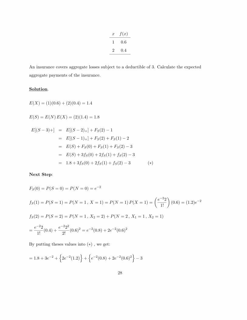
x f(x)

1 0.6

2 0.4

An insurance covers aggregate losses subject to a deductible of 3. Calculate the expected

aggregate payments of the insurance.

Solution.

E(X) = (1)(0.6) + (2)(0.4) = 1.4

E(S) = E(N)E(X) = (2)(1.4) = 1.8

E[(S − 3)+] = E[(S − 2)+] + FS(2)− 1

= E[(S − 1)+] + FS(2) + FS(1)− 2

= E(S) + FS(0) + FS(1) + FS(2)− 3

= E(S) + 3fS(0) + 2fS(1) + fS(2)− 3

= 1.8 + 3fS(0) + 2fS(1) + fS(2)− 3 (∗)

Next Step:

FS(0) = P (S = 0) = P (N = 0) = e−2

fS(1) = P (S = 1) = P (N = 1 , X = 1) = P (N = 1)P (X = 1) =

(e−22

1!

)(0.6) = (1.2)e−2

fS(2) = P (S = 2) = P (N = 1 , X2 = 2) + P (N = 2 , X1 = 1 , X2 = 1)

=e−22

1!(0.4) +

e−222

2!(0.6)2 = e−2(0.8) + 2e−2(0.6)2

By putting theses values into (∗) , we get:

= 1.8 + 3e−2 +2e−2(1.2)

+

e−2(0.8) + 2e−2(0.6)2

− 3

28

= −1.2 + 6.92 e−2

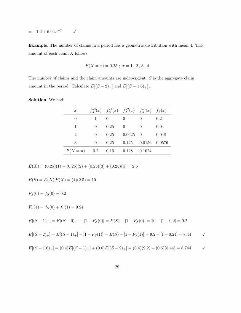
Example. The number of claims in a period has a geometric distribution with mean 4. The

amount of each claim X follows

P (X = x) = 0.25 ; x = 1 , 2 , 3 , 4

The number of claims and the claim amounts are independent. S is the aggregate claim

amount in the period. Calculate E[(S − 2)+] and E[(S − 1.6)+] .

Solution. We had:

x f∗0X (x) f∗1

X (x) f∗2X (x) f∗3

X (x) fS(x)

0 1 0 0 0 0.2

1 0 0.25 0 0 0.04

2 0 0.25 0.0625 0 0.048

3 0 0.25 0.125 0.0156 0.0576

P (N = n) 0.2 0.16 0.128 0.1024

E(X) = (0.25)(1) + (0.25)(2) + (0.25)(3) + (0.25)(4) = 2.5

E(S) = E(N)E(X) = (4)(2.5) = 10

FS(0) = fS(0) = 0.2

FS(1) = fS(0) + fS(1) = 0.24

E[(S − 1)+] = E[(S − 0)+]− [1− FS(0)] = E(S)− [1− FS(0)] = 10− [1− 0.2] = 9.2

E[(S − 2)+] = E[(S − 1)+]− [1− FS(1)] = E(S)− [1− FS(1)] = 9.2− [1− 0.24] = 8.44

E[(S − 1.6)+] = (0.4)E[(S − 1)+] + (0.6)E[(S − 2)+] = (0.4)(9.2) + (0.6)(8.44) = 8.744

29

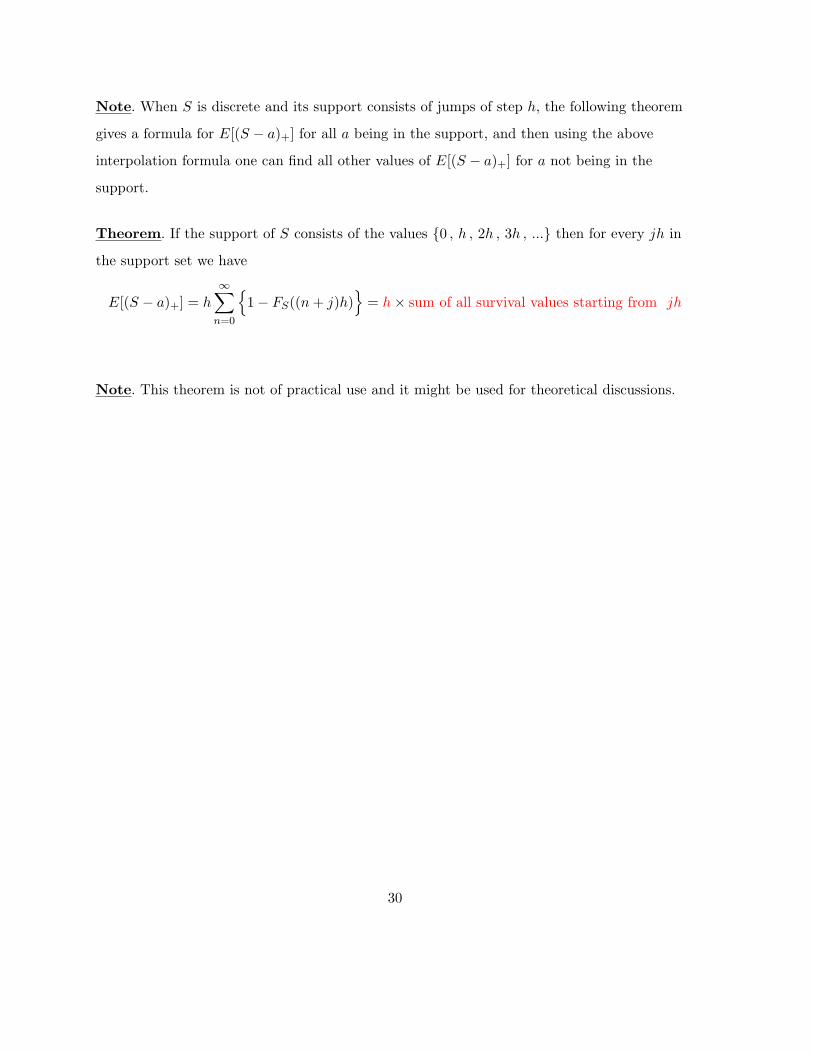
Note. When S is discrete and its support consists of jumps of step h, the following theorem

gives a formula for E[(S − a)+] for all a being in the support, and then using the above

interpolation formula one can find all other values of E[(S − a)+] for a not being in the

support.

Theorem. If the support of S consists of the values 0 , h , 2h , 3h , ... then for every jh in

the support set we have

E[(S − a)+] = h

∞∑n=0

1− FS((n+ j)h)

= h× sum of all survival values starting from jh

Note. This theorem is not of practical use and it might be used for theoretical discussions.

30

Panjer Recursive Formulas

section 9.6

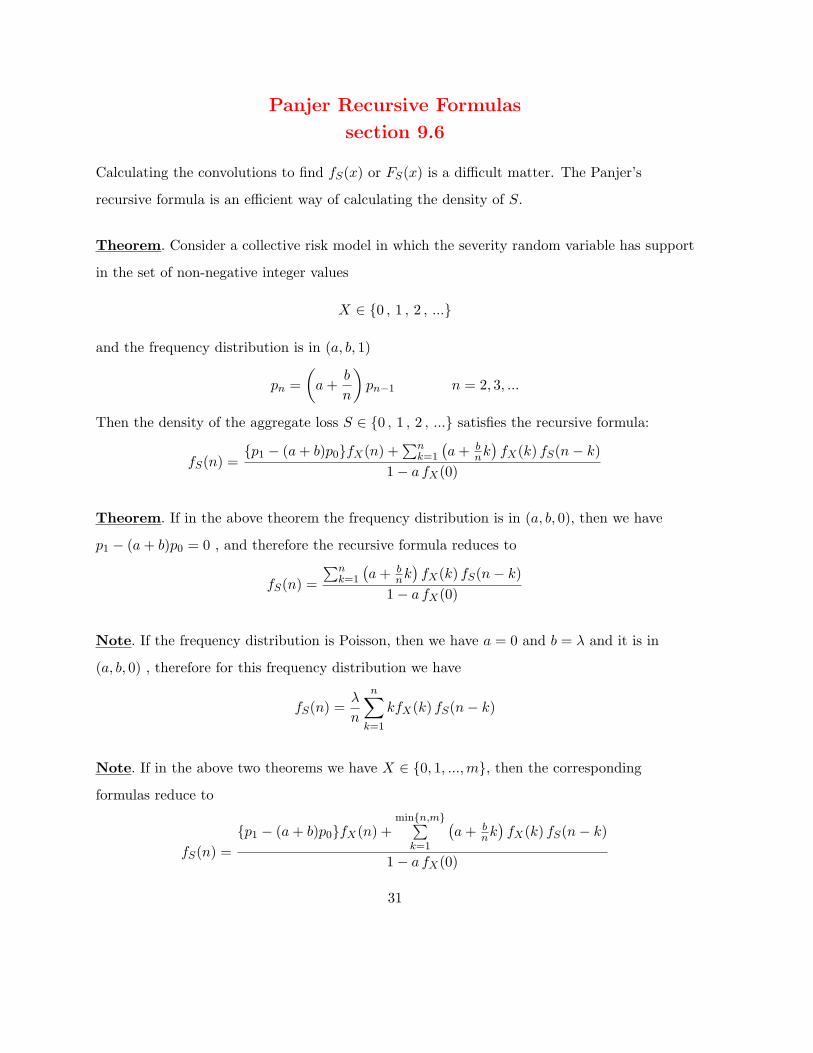
Calculating the convolutions to find fS(x) or FS(x) is a difficult matter. The Panjer’s

recursive formula is an efficient way of calculating the density of S.

Theorem. Consider a collective risk model in which the severity random variable has support

in the set of non-negative integer values

X ∈ 0 , 1 , 2 , ...

and the frequency distribution is in (a, b, 1)

pn =

(a+

b

n

)pn−1 n = 2, 3, ...

Then the density of the aggregate loss S ∈ 0 , 1 , 2 , ... satisfies the recursive formula:

fS(n) =p1 − (a+ b)p0fX(n) +

∑nk=1

(a+ b

nk)fX(k) fS(n− k)

1− a fX(0)

Theorem. If in the above theorem the frequency distribution is in (a, b, 0), then we have

p1 − (a+ b)p0 = 0 , and therefore the recursive formula reduces to

fS(n) =

∑nk=1

(a+ b

nk)fX(k) fS(n− k)

1− a fX(0)

Note. If the frequency distribution is Poisson, then we have a = 0 and b = λ and it is in

(a, b, 0) , therefore for this frequency distribution we have

fS(n) =λ

n

n∑k=1

kfX(k) fS(n− k)

Note. If in the above two theorems we have X ∈ 0, 1, ...,m, then the corresponding

formulas reduce to

fS(n) =

p1 − (a+ b)p0fX(n) +minn,m∑

k=1

(a+ b

nk)fX(k) fS(n− k)

1− a fX(0)

31

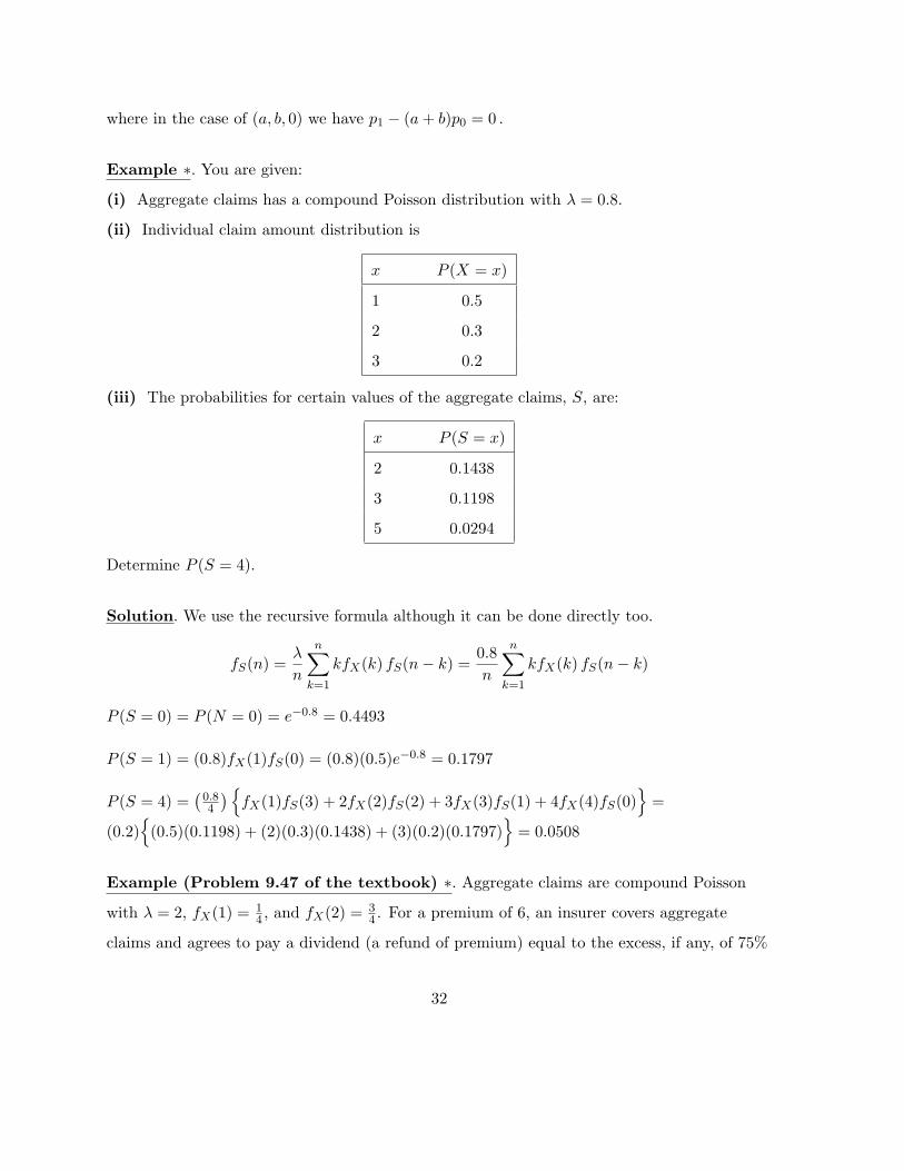
where in the case of (a, b, 0) we have p1 − (a+ b)p0 = 0 .

Example ∗. You are given:

(i) Aggregate claims has a compound Poisson distribution with λ = 0.8.

(ii) Individual claim amount distribution is

x P (X = x)

1 0.5

2 0.3

3 0.2

(iii) The probabilities for certain values of the aggregate claims, S, are:

x P (S = x)

2 0.1438

3 0.1198

5 0.0294

Determine P (S = 4).

Solution. We use the recursive formula although it can be done directly too.

fS(n) =λ

n

n∑k=1

kfX(k) fS(n− k) =0.8

n

n∑k=1

kfX(k) fS(n− k)

P (S = 0) = P (N = 0) = e−0.8 = 0.4493

P (S = 1) = (0.8)fX(1)fS(0) = (0.8)(0.5)e−0.8 = 0.1797

P (S = 4) =(0.84

)fX(1)fS(3) + 2fX(2)fS(2) + 3fX(3)fS(1) + 4fX(4)fS(0)

=

(0.2)(0.5)(0.1198) + (2)(0.3)(0.1438) + (3)(0.2)(0.1797)

= 0.0508

Example (Problem 9.47 of the textbook) ∗. Aggregate claims are compound Poisson

with λ = 2, fX(1) = 14 , and fX(2) = 3

4 . For a premium of 6, an insurer covers aggregate

claims and agrees to pay a dividend (a refund of premium) equal to the excess, if any, of 75%

32

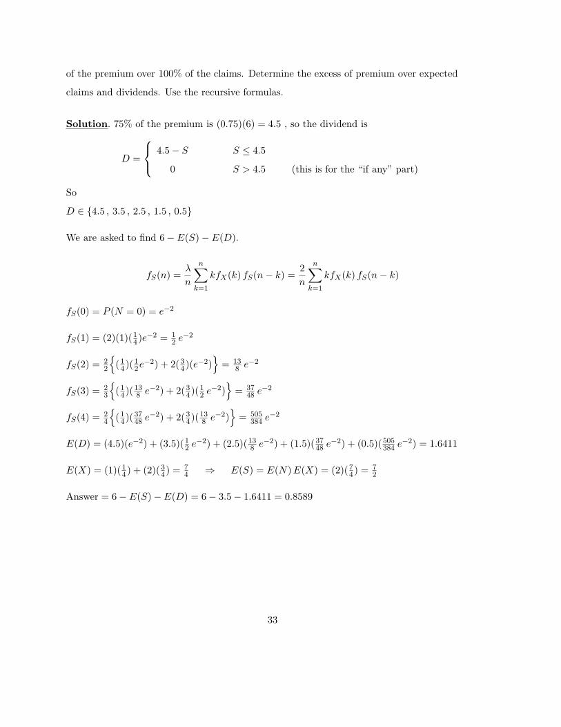
of the premium over 100% of the claims. Determine the excess of premium over expected

claims and dividends. Use the recursive formulas.

Solution. 75% of the premium is (0.75)(6) = 4.5 , so the dividend is

D =

4.5− S S ≤ 4.5

0 S > 4.5 (this is for the “if any” part)

So

D ∈ 4.5 , 3.5 , 2.5 , 1.5 , 0.5

We are asked to find 6− E(S)− E(D).

fS(n) =λ

n

n∑k=1

kfX(k) fS(n− k) =2

n

n∑k=1

kfX(k) fS(n− k)

fS(0) = P (N = 0) = e−2

fS(1) = (2)(1)(14)e−2 = 1

2 e−2

fS(2) =22

(14)(

12e

−2) + 2(34)(e−2)

= 13

8 e−2

fS(3) =23

(14)(

138 e−2) + 2(34)(

12 e

−2)= 37

48 e−2

fS(4) =24

(14)(

3748 e

−2) + 2(34)(138 e−2)

= 505

384 e−2

E(D) = (4.5)(e−2) + (3.5)(12 e−2) + (2.5)(138 e−2) + (1.5)(3748 e

−2) + (0.5)(505384 e−2) = 1.6411

E(X) = (1)(14) + (2)(34) =74 ⇒ E(S) = E(N)E(X) = (2)(74) =

72

Answer = 6− E(S)− E(D) = 6− 3.5− 1.6411 = 0.8589

33