AGA CALCULATIONS — OLD VS NEWmeter. In particular orifice plates, plate holders, sensing taps,...
18
PAGE 172 2002 PROCEEDINGS AMERICAN SCHOOL OF GAS MEASUREMENT TECHNOLOGY C d Y π d 2 2g c ρ f ∆P 1–β 4 4 Q V = ρ b AGA CALCULATIONS — OLD VS NEW Brent E. Berry ABB-Totalflow Pawhusk Road, Bartlesville, OK 74005 SECTION 1 — BACKGROUND This paper is intended to help bridge the gap between the Old AGA-3 equation (hereafter referred to as AGA- 3-1985) and the New AGA-3 equation (hereafter referred to as AGA-3-1992). As such the paper begins with a background section aimed at assisting those who are mostly familiar with the factored form of the orifice metering equation. Factored VS Fundamental Flow Rate Equation Form Of the following two equations, which are published in the AGA-3-1985 standard? (a) equation 1 (b) equation 2 (c) both equation 1 and 2 (d) don’t know (eq 1) where, (eq 2) The correct answer is (c). Both equations are actually published in the 1985 standard and they are both equivalent within their scope of applicability. Equation 2 is often referred to as the factored form of the AGA-3 equation. It can be found on page 38 of the 1985 standard as equations (59) and (60). Equation 1 is the fundamental orifice meter equation. It can be found on page 25 of the 1985 standard and is actually a combination of equations (3) and (7) on that page. Equation 1 describes the theoretical basis, the physical and practical realities of an orifice flow meter. Equation 2, the factored equation, is based on or derived from equation 1. Why bring all this up now? If you are like this author was at one time, you might only be familiar with the factored equation. If so, I recommended you become more familiar with the fundamental form of the equation. Firstly, because this form more readily facilitates comparing AGA-3-1985 and AGA-3-1992. Secondly, you will be more comfortable with the new AGA-3-1992 standard. Thirdly, because it more clearly describes orifice meter dynamics. Why are there different forms of the equation anyway? The first factored form of the equation was introduced in 1935 with the publication of Gas Measurement Com- mittee Report No. 2. Before that time the factors were not in use. Factors are a convention that allow various terms of the fundamental equation to be calculated individually. This allows tables to be generated for each factor which can then be used to estimate volumes. These tables were especially useful before the availability of computers and programmable calculators. They are still used and will continue to be used, but their usage is diminishing with the advent of electronic instrumentation. C d , Coefficient of Discharge If the old factored equation is all you have been using, you may have never really dealt with C d . Basically, C d is imbedded in the old factored equation as part of (F b * F r ). Reviewing equation 1 of this document you will notice C d is included as part of AGA-3-1985’s fundamental equa- tion. It has always been there, simply hidden by the factors. Most of the research and development undertaken over the last several years was for the purpose of deriving a more accurate, technically defensible correlation between a published C d equation and actual laboratory data. This is at the heart of the changes in AGA-3-1992. What is the purpose of C d in the fundamental equation? C d = true flow ratesp pi theoretical flow rate The true flow rate is determined in a laboratory by weighing or by volumetric collection of the fluid over a measured time interval and the theoretical flow rate is calculated. Then a discharge coefficient (C d ) is computed as a correction factor to the theoretical flow rate. This data is all generated over varying flow rates, fluid types (Reynolds number conditions) and various geometries (diameters). Once all the data is taken then an empirical equation is derived which allows us to compute C d over many combinations of conditions. That is what C d , the coefficient of discharge is. It is a high falutin’ fudge factor. The developers of the new equation have taken advantage of newer technology in more numerous testing labs to gather more real world data over a wider set of operating conditions. They have also postulated on a new form of the C d equation that they believe more closely correlates to the fluid dynamics associated with the physics of an orifice meter. This means the new C d is based more on first principles than the older one. You might say it has a higher falutin’ index than the older coefficient of discharge. C ’ = F b F r Y F pb F tb F tf F gr F pv Q v = C’ h w P f
Transcript of AGA CALCULATIONS — OLD VS NEWmeter. In particular orifice plates, plate holders, sensing taps,...
PAGE 172 2002 PROCEEDINGSAMERICAN SCHOOL OF GAS MEASUREMENT TECHNOLOGY
Cd Y π d 2 2 gcρ
f∆P
1–β4 4Q
V = ρ
b
AGA CALCULATIONS — OLD VS NEWBrent E. BerryABB-Totalflow
Pawhusk Road, Bartlesville, OK 74005
SECTION 1 — BACKGROUND
This paper is intended to help bridge the gap betweenthe Old AGA-3 equation (hereafter referred to as AGA-3-1985) and the New AGA-3 equation (hereafter referredto as AGA-3-1992). As such the paper begins with abackground section aimed at assisting those who aremostly familiar with the factored form of the orificemetering equation.
Factored VS Fundamental Flow Rate Equation Form
Of the following two equations, which are published inthe AGA-3-1985 standard?
(a) equation 1(b) equation 2(c) both equation 1 and 2(d) don’t know
(eq 1)
where,
(eq 2)
The correct answer is (c). Both equations are actuallypublished in the 1985 standard and they are bothequivalent within their scope of applicability. Equation 2is often referred to as the factored form of the AGA-3equation. It can be found on page 38 of the 1985standard as equations (59) and (60). Equation 1 is thefundamental orifice meter equation. It can be found onpage 25 of the 1985 standard and is actually acombination of equations (3) and (7) on that page.
Equation 1 describes the theoretical basis, the physicaland practical realities of an orifice flow meter. Equation2, the factored equation, is based on or derived fromequation 1. Why bring all this up now? If you are like thisauthor was at one time, you might only be familiar withthe factored equation. If so, I recommended you becomemore familiar with the fundamental form of the equation.Firstly, because this form more readily facilitatescomparing AGA-3-1985 and AGA-3-1992. Secondly, youwill be more comfortable with the new AGA-3-1992standard. Thirdly, because it more clearly describesorifice meter dynamics.
Why are there different forms of the equation anyway?The first factored form of the equation was introducedin 1935 with the publication of Gas Measurement Com-mittee Report No. 2. Before that time the factors werenot in use. Factors are a convention that allow variousterms of the fundamental equation to be calculatedindividually. This allows tables to be generated for eachfactor which can then be used to estimate volumes.These tables were especially useful before the availabilityof computers and programmable calculators. They arestill used and will continue to be used, but their usage isdiminishing with the advent of electronic instrumentation.
Cd, Coefficient of Discharge
If the old factored equation is all you have been using, youmay have never really dealt with Cd. Basically, Cd isimbedded in the old factored equation as part of (Fb * Fr).Reviewing equation 1 of this document you will notice Cd
is included as part of AGA-3-1985’s fundamental equa-tion. It has always been there, simply hidden by the factors.Most of the research and development undertaken overthe last several years was for the purpose of deriving amore accurate, technically defensible correlation betweena published Cd equation and actual laboratory data. Thisis at the heart of the changes in AGA-3-1992.
What is the purpose of Cd in the fundamental equation?
Cd = true flow ratesppi
theoretical flow rate
The true flow rate is determined in a laboratory byweighing or by volumetric collection of the fluid over ameasured time interval and the theoretical flow rate iscalculated. Then a discharge coefficient (Cd) is computedas a correction factor to the theoretical flow rate. Thisdata is all generated over varying flow rates, fluid types(Reynolds number conditions) and various geometries(diameters). Once all the data is taken then an empiricalequation is derived which allows us to compute Cd overmany combinations of conditions.
That is what Cd, the coefficient of discharge is. It is ahigh falutin’ fudge factor. The developers of the newequation have taken advantage of newer technology inmore numerous testing labs to gather more real worlddata over a wider set of operating conditions. They havealso postulated on a new form of the Cd equation thatthey believe more closely correlates to the fluid dynamicsassociated with the physics of an orifice meter. Thismeans the new Cd is based more on first principles thanthe older one. You might say it has a higher falutin’ indexthan the older coefficient of discharge.
C ’ = Fb Fr Y Fpb Ftb Ftf Fgr Fpv
Qv = C’ hw Pf

2002 PROCEEDINGS PAGE 173AMERICAN SCHOOL OF GAS MEASUREMENT TECHNOLOGY
Why does the theoretical equation not match the realworld exactly?
In trying to keep orifice metering practical, simplifyingassumptions are sometimes made. It is simply not alwayspossible, practical or necessary to perfectly model thereal world. Some of the things influencing the theoreticalequation, causing it not to model the real world exactlyare:
(1) It is assumed there is no energy loss between thetaps.
(2) The velocity profile (Reynolds number) influences arenot fully treated by the equation. It is assumed thatsome installation effects and causes of flow pertur-bations (changes) are insignificant.
(3) Different tap locations affect the flow rate. Taplocation is assumed for a given Cd.
Through rigorous testing, you could develop a uniqueCd for each of your orifice meters. This technique, referredto as in-situ calibration, is something like proving a linearmeter. However it is somewhat bothersome since youneed a unique Cd for each expected flow rate. Economicsusually make in-situ procedures unfeasible.
Therefore, the goal is to develop a universal Cd thateveryone can use. To accomplish this, one must controltheir orifice meter installation well enough so that itreplicates the same orifice meters used in the laboratoryfrom which the universal Cd equation was derived. Thisis referred to as the law of similarity. If your orifice metersystem is acceptably similar to the laboratory’s then yourCd will be acceptably similar to the laboratory derivedCd. That is why edge sharpness, wall roughness,eccentricity and flow conditioning, etc. are so important.Ideally your flow measurement system would be exactlythe same as was used in the laboratory.
Density
If the old factored equation is all you have been using,you may have never really dealt with density. Lookingback at Equation 1 of this document you will notice twosymbols, ρf and ρb. The symbol ρ (pronounced rho) isused to represent density.ρf = density at flowing conditionsρb = density at base conditions
Most measurement systems do not have density as alive input, so density is computed from other data that isavailable. When the fluid being measured is a gas, densityis computed from other data as follows:
Density at Flowing Conditions
(eq. 3)
Density at Base Conditions
(eq. 4)
Notice Pf, Tf, Zf, Gi, Pb, Tb, and Zb in eq 3 and eq 4. Theserepresent temperatures, pressures, specific gravities andcompressibilities. It is these variables that eventuallymake there way into the old factors Ftb, Fpb, Ftf, Fgr, andFpv (see Section 3 of this document for more information).Leaving densities in the fundamental equation, ratherthan hiding them in a plethora (abundance) of factors,seems less confusing and more instructive.
Real VS Ideal Gas Specific Gravity
One other item of note regarding the density equationsis that they are based on Gi, ideal gas specific gravity.Most systems have historically provided Gr, real gasspecific gravity, which is different. Additionally AGA-8requires Gr as an input, not Gi. Strictly speaking,Gi isrelated to Gr with the following equation.
Practically speaking the measurement system does notusually have enough information available to solve theabove equation. Part 3 of the new standard makes thefollowing statements regarding this issue.
“the pressures and temperatures are defined to be atthe same designated base conditions....”. And again in afollowing paragraph, “The fact that the temperature and/or pressure are not always at base conditions results insmall variations in determinations of relative density(specific gravity). Another source of variation is the useof atmospheric air. The composition of atmospheric air —and its molecular weight and density — varies with timeand geographical location.” 3
Based on this, and several of the examples in the stan-dard, the following simplifying assumptions are made:
(eq. 5)
This equation for Gi is exactly like the one shown asequation 3-48 on page 19 of Part 3 of the new standard.
PAGE 174 2002 PROCEEDINGSAMERICAN SCHOOL OF GAS MEASUREMENT TECHNOLOGY
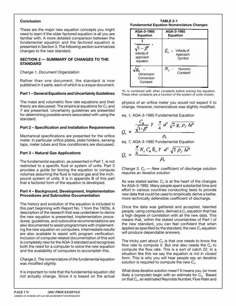
Conclusion
These are the major new equation concepts you mightneed to learn if the older factored equation is all you arefamiliar with. A more detailed comparison between thefundamental equation and the factored equation ispresented in Section 3. The following section summarizeschanges to the new standard.
SECTION 2 — SUMMARY OF CHANGES TO THESTANDARD
Change 1, Document Organization
Rather than one document, the standard is nowpublished in 4 parts, each of which is a unique document.
Part 1 – General Equations and Uncertainty Guidelines
The mass and volumetric flow rate equations and theirtheory are discussed. The empirical equations for Cd andY are presented. Uncertainty guidelines are presentedfor determining possible errors associated with using thestandard.
Part 2 – Specification and Installation Requirements
Mechanical specifications are presented for the orificemeter. In particular orifice plates, plate holders, sensingtaps, meter tubes and flow conditioners are discussed.
Part 3 – Natural Gas Applications
The fundamental equation, as presented in Part 1, is notrestricted to a specific fluid or system of units. Part 3provides a guide for forcing the equation to computevolumes assuming the fluid is natural gas and the inch-pound system of units. It is in appendix B of this partthat a factored form of the equation is developed.
Part 4 – Background, Development, ImplementationProcedures and Subroutine Documentation
The history and evolution of the equation is included inthis part beginning with Report No. 1 from the 1920s. Adescription of the research that was undertaken to derivethe new equation is presented. Implementation proce-dures, guidelines, and subroutine recommendations arealso documented to assist programmers with implement-ing the new equation on computers. Intermediate resultsare also available to assist with program verification.Inclusion of computer related documentation of this sortis completely new for the AGA-3 standard and recognizesboth the need for a computer to solve the new equationand the availability of computers to accomplish this.
Change 2, The nomenclature of the fundamental equationwas modified slightly.
It is important to note that the fundamental equation didnot actually change. Since it is based on the actual
physics of an orifice meter you would not expect it tochange. However, nomenclature was slightly modified.
eq. 1, AGA-3-1985 Fundamental Equation
eq. 7, AGA-3-1992 Fundamental Equation
Change 3, Cd — New coefficient of discharge solutionrequires an iterative solution
As was stated earlier, Cd is at the heart of the changesfor AGA-3-1992. Many people spent substantial time andeffort in various countries conducting tests to providenew data that could be used to empirically derive a better,more technically defensible coefficient of discharge.
Once the data was gathered and accepted, talentedpeople, using computers, derived a Cd equation that hasa high degree of correlation with all the new data. Thismeans that, within the stated uncertainties of Part I ofthe new standard, you can feel confident that whenapplied as specified by the standard, the new Cd equationwill produce dependable answers.
The tricky part about Cd is that one needs to know theflow rate to compute it. But one also needs the Cd tocompute the flow rate. This is a sort of catch 22. In asituation like this we say the equation is not in closedform. This is why you will hear people say an iterativesolution is required to compute the new Cd.
What does iterative solution mean? It means you, (or morelikely a computer) begin with an estimate for Cd. Basedon that Cd, an estimated Reynolds Number, Flow Rate and
TABLE 2-1Fundamental Equation Nomenclature Changes
AGA-3-1992Equation
AGA-3-1985Equation
NumericConstant*Dimension
ConversionConstant
velocity ofapproachequation
Velocity ofApproachSymbol
*Nc is combined with other constants before solving the equation.These other constants are a function of the system of units chosen.

2002 PROCEEDINGS PAGE 175AMERICAN SCHOOL OF GAS MEASUREMENT TECHNOLOGY
a subsequent new Cd are computed. The two Cd values(Cd_old and Cd_new ) are compared and if they differ bymore than an acceptable threshold, the process isrepeated. Each time the process is repeated the mostrecent Cd is retained for comparison with the next onebeing computed. Eventually, the difference betweenCd_old and Cd_new become so small it is safe toassume the proper Cd value has been obtained. APIdesigners estimate that, most of the time, no more thanthree iterations will be required. I believe no more than10 iterations were ever required on the test cases. Anexact procedure is outlined in Part 4 of the new standardunder Procedure 4.3.2.9. In that procedure the thresholdfor determining acceptable convergence is six significantdigits (0.000005).
Change 4, Thermal effect corrections on Pipe and Orificediameters are required
In the AGA-3-1985 standard an optional orifice thermalexpansion factor, Fa, was specified to correct for the errorresulting from thermal effects on the orifice plate diameter.
In the AGA-3-1992 standard this type of correction isnot optional. It is required. Additionally you must alsomake corrections for thermal effects on the pipe diameter.
Another new requirement is that these corrections cannotbe tacked onto the end of the equation as a factor. Theyare to be applied on the front end as adjustments to thediameters themselves. Therefore, the end user shouldbe supplying diameters at a reference temperature(68 DegF), and the device solving the equation shouldbe adjusting the diameters based on the differencebetween the reference temperature and the actual fluidtemperature.
This means that virtually none of the equation can be pre-computed and re-used. Even though the new equationdoes not have Fb, there are portions of the equation thatdepend only on the diameters. In the past, we would com-pute those portions of the equation only when thediameters manually changed. Now, since the diametersare a function of temperature they, and everything basedon them, must be computed on a continual basis.
Assume the measurement system is supplied dr, orificediameter at reference temperature and Dr, pipe diameterand reference temperature. Before these diameters canbe used anywhere in the flow rate calculation they mustbe corrected for thermal effects with the followingequations.
Corrected orifice diameter
Corrected pipe diameter
Change 5, Downstream expansion factor, requiresadditional compressibility
The equations for upstream expansion factor have notchanged. However to compute the downstreamexpansion factor, real gas effects must now be accountedfor. This means an additional Z, compressibilitycalculation is required when computing the downstreamexpansion factor.
If your system measures static pressure downstream,but you do not want to incur the additional processingto compute another Z for the expansion factor, there issomething you can do.
You can compute the upstream pressure as follows anduse it to compute the upstream expansion factor.
where N is a conversion constant from differentialpressure to static pressure units.
If you employ this technique, you must be careful to usePf1 for all occurrences of static pressure in the flow rateequation. You cannot use upstream pressure in someplaces and downstream pressure in others.
Change 6, Fpv, supercompressibility is computed usingAGA-8
Many people have been using NX-19 to compute Fpv fornatural gas. The new standard specifies AGA-8.
A new AGA-8 standard was published in late 1992. Thatstandard documents two possible ways to compute Fpv.One method is referred to as gross method, the other isreferred to as detailed method. The gross method issupposed to be simpler to implement and require lesscomputing power than the detailed method. Havingworked with both, I can tell you that compared to eitherof these methods NX-19 processing requirements arerelatively minuscule (small).
As a user, there are two major distinctions between thegross and detailed methods you should consider.
1. The gross method accepts the same compositiondata you are used to supplying for NX-19 (specificgravity, percent CO2 and N2). The detailed methodrequires a total analysis. What constitutes a totalanalysis depends on each measurement site.Generally, composition through C6s is considered atotal analysis. Sometimes C7s or C8s or C9s mightneed to be broken out. The detailed method of theequation will support this if needed.
2. The gross method is applicable over a narrowerrange of operating conditions than the detailedmethod. The gross method was designed to beapplicable for pipeline quality natural gas at normal
PAGE 176 2002 PROCEEDINGSAMERICAN SCHOOL OF GAS MEASUREMENT TECHNOLOGY
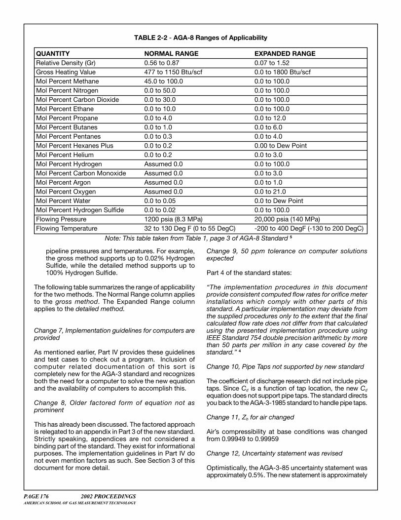
pipeline pressures and temperatures. For example,the gross method supports up to 0.02% HydrogenSulfide, while the detailed method supports up to100% Hydrogen Sulfide.
The following table summarizes the range of applicabilityfor the two methods. The Normal Range column appliesto the gross method. The Expanded Range columnapplies to the detailed method.
Change 7, Implementation guidelines for computers areprovided
As mentioned earlier, Part IV provides these guidelinesand test cases to check out a program. Inclusion ofcomputer related documentation of this sort iscompletely new for the AGA-3 standard and recognizesboth the need for a computer to solve the new equationand the availability of computers to accomplish this.
Change 8, Older factored form of equation not asprominent
This has already been discussed. The factored approachis relegated to an appendix in Part 3 of the new standard.Strictly speaking, appendices are not considered abinding part of the standard. They exist for informationalpurposes. The implementation guidelines in Part IV donot even mention factors as such. See Section 3 of thisdocument for more detail.
Change 9, 50 ppm tolerance on computer solutionsexpected
Part 4 of the standard states:
“The implementation procedures in this documentprovide consistent computed flow rates for orifice meterinstallations which comply with other parts of thisstandard. A particular implementation may deviate fromthe supplied procedures only to the extent that the finalcalculated flow rate does not differ from that calculatedusing the presented implementation procedure usingIEEE Standard 754 double precision arithmetic by morethan 50 parts per million in any case covered by thestandard.” 4
Change 10, Pipe Taps not supported by new standard
The coefficient of discharge research did not include pipetaps. Since Cd is a function of tap location, the new Cd
equation does not support pipe taps. The standard directsyou back to the AGA-3-1985 standard to handle pipe taps.
Change 11, Zb for air changed
Air’s compressibility at base conditions was changedfrom 0.99949 to 0.99959
Change 12, Uncertainty statement was revised
Optimistically, the AGA-3-85 uncertainty statement wasapproximately 0.5%. The new statement is approximately
TABLE 2-2 - AGA-8 Ranges of Applicability
QUANTITY NORMAL RANGE EXPANDED RANGERelative Density (Gr) 0.56 to 0.87 0.07 to 1.52Gross Heating Value 477 to 1150 Btu/scf 0.0 to 1800 Btu/scfMol Percent Methane 45.0 to 100.0 0.0 to 100.0Mol Percent Nitrogen 0.0 to 50.0 0.0 to 100.0Mol Percent Carbon Dioxide 0.0 to 30.0 0.0 to 100.0Mol Percent Ethane 0.0 to 10.0 0.0 to 100.0Mol Percent Propane 0.0 to 4.0 0.0 to 12.0Mol Percent Butanes 0.0 to 1.0 0.0 to 6.0Mol Percent Pentanes 0.0 to 0.3 0.0 to 4.0Mol Percent Hexanes Plus 0.0 to 0.2 0.00 to Dew PointMol Percent Helium 0.0 to 0.2 0.0 to 3.0Mol Percent Hydrogen Assumed 0.0 0.0 to 100.0Mol Percent Carbon Monoxide Assumed 0.0 0.0 to 3.0Mol Percent Argon Assumed 0.0 0.0 to 1.0Mol Percent Oxygen Assumed 0.0 0.0 to 21.0Mol Percent Water 0.0 to 0.05 0.0 to Dew PointMol Percent Hydrogen Sulfide 0.0 to 0.02 0.0 to 100.0Flowing Pressure 1200 psia (8.3 MPa) 20,000 psia (140 MPa)Flowing Temperature 32 to 130 Deg F (0 to 55 DegC) -200 to 400 DegF (-130 to 200 DegC)
Note: This table taken from Table 1, page 3 of AGA-8 Standard 5
2002 PROCEEDINGS PAGE 177AMERICAN SCHOOL OF GAS MEASUREMENT TECHNOLOGY
0.5% for Cd plus uncertainty in other measured variables.Typical is probably between 0.6% and 0.7%.
This may sound as if the new equation has as muchuncertainty as the old. However, it appears the AGA-3-1985 uncertainty statement was very optimist and, strictlyspeaking, was not technically defensible over all theoperating conditions for which it was being used.
The new standard is expected to improve the uncertaintyby 0.1% - 0.5%. 6
Regarding this issue, a summary of statements takenfrom Part 4 of the new standard follows:
The orifice equation in use through AGA-3-1985 wasbased on data collected in 1932/33 under the directionof Professor S.R. Beitler at Ohio State University (OSU).The results of these experiments were used by Dr. EdgarBuckingham and Mr. Howard Bean to develop thecoefficient of discharge equation.
In the 1970’s, researchers reevaluated the OSU data andfound a number of reasons to question some of the datapoints. This analysis identified 303 technically defensibledata points from the OSU experiments. Unfortunately itis not known which points were used by Buckingham/Bean to generate the discharge coefficient equation.
Statistical analysis of the Regression Data Set (the newdata set) showed that in several regions, the Buckingham/Bean equations did not accurately represent that data.4
This means that the uncertainty statement in the AGA-3-1985 standard cannot be substantiated in all cases.
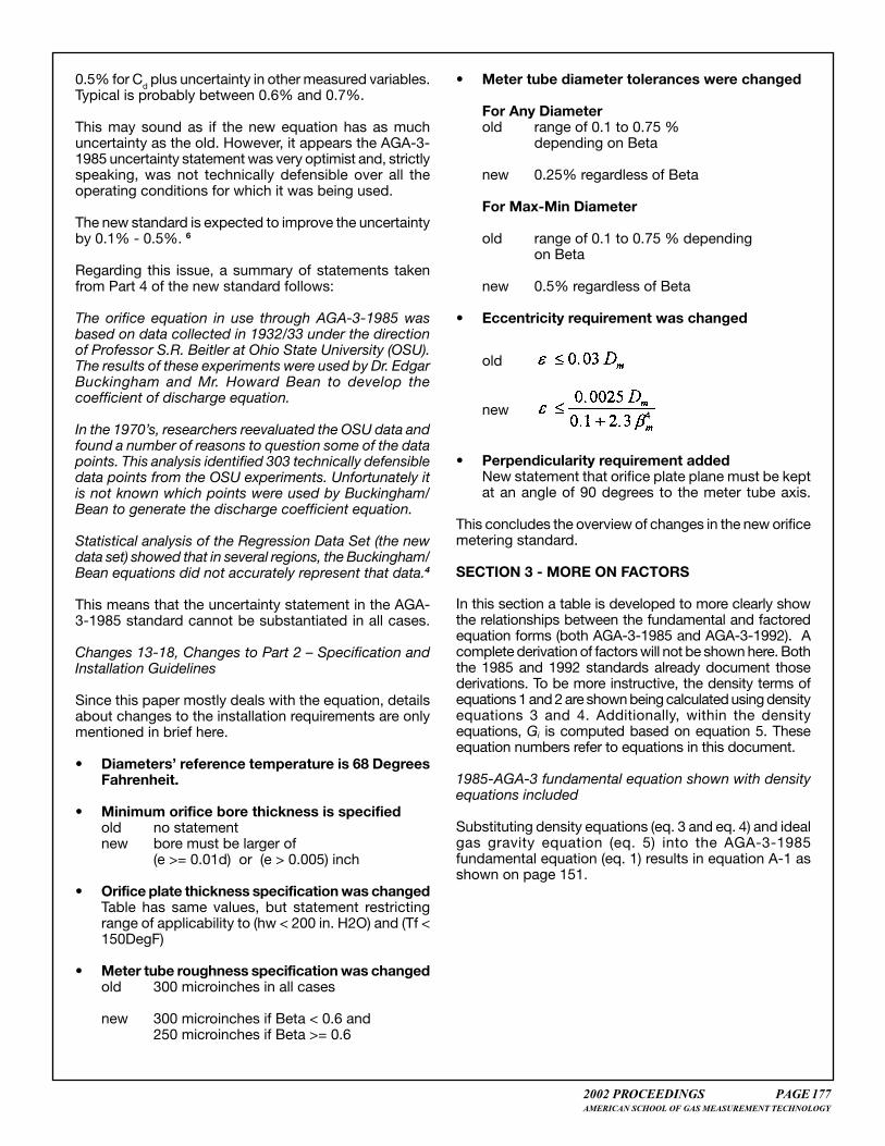
Changes 13-18, Changes to Part 2 – Specification andInstallation Guidelines
Since this paper mostly deals with the equation, detailsabout changes to the installation requirements are onlymentioned in brief here.
• Diameters’ reference temperature is 68 DegreesFahrenheit.
• Minimum orifice bore thickness is specifiedold no statementnew bore must be larger of
(e >= 0.01d) or (e > 0.005) inch
• Orifice plate thickness specification was changedTable has same values, but statement restrictingrange of applicability to (hw < 200 in. H2O) and (Tf <150DegF)
• Meter tube roughness specification was changedold 300 microinches in all cases
new 300 microinches if Beta < 0.6 and250 microinches if Beta >= 0.6
• Meter tube diameter tolerances were changed
For Any Diameterold range of 0.1 to 0.75 %
depending on Beta
new 0.25% regardless of Beta
For Max-Min Diameter
old range of 0.1 to 0.75 % dependingon Beta
new 0.5% regardless of Beta
• Eccentricity requirement was changed
old
new
• Perpendicularity requirement addedNew statement that orifice plate plane must be keptat an angle of 90 degrees to the meter tube axis.
This concludes the overview of changes in the new orificemetering standard.
SECTION 3 - MORE ON FACTORS
In this section a table is developed to more clearly showthe relationships between the fundamental and factoredequation forms (both AGA-3-1985 and AGA-3-1992). Acomplete derivation of factors will not be shown here. Boththe 1985 and 1992 standards already document thosederivations. To be more instructive, the density terms ofequations 1 and 2 are shown being calculated using densityequations 3 and 4. Additionally, within the densityequations, Gi is computed based on equation 5. Theseequation numbers refer to equations in this document.
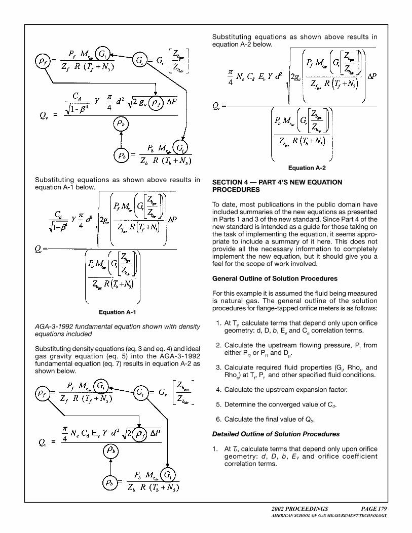
1985-AGA-3 fundamental equation shown with densityequations included
Substituting density equations (eq. 3 and eq. 4) and idealgas gravity equation (eq. 5) into the AGA-3-1985fundamental equation (eq. 1) results in equation A-1 asshown on page 151.
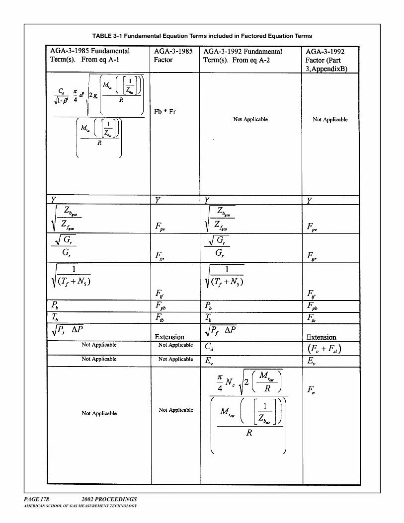
PAGE 178 2002 PROCEEDINGSAMERICAN SCHOOL OF GAS MEASUREMENT TECHNOLOGY
TABLE 3-1 Fundamental Equation Terms included in Factored Equation Terms
2002 PROCEEDINGS PAGE 179AMERICAN SCHOOL OF GAS MEASUREMENT TECHNOLOGY
Substituting equations as shown above results inequation A-1 below.
Equation A-1
AGA-3-1992 fundamental equation shown with densityequations included
Substituting density equations (eq. 3 and eq. 4) and idealgas gravity equation (eq. 5) into the AGA-3-1992fundamental equation (eq. 7) results in equation A-2 asshown below.
Substituting equations as shown above results inequation A-2 below.
Equation A-2
SECTION 4 — PART 4’S NEW EQUATIONPROCEDURES
To date, most publications in the public domain haveincluded summaries of the new equations as presentedin Parts 1 and 3 of the new standard. Since Part 4 of thenew standard is intended as a guide for those taking onthe task of implementing the equation, it seems appro-priate to include a summary of it here. This does notprovide all the necessary information to completelyimplement the new equation, but it should give you afeel for the scope of work involved.
General Outline of Solution Procedures
For this example it is assumed the fluid being measuredis natural gas. The general outline of the solutionprocedures for flange-tapped orifice meters is as follows:
1. At Tf, calculate terms that depend only upon orificegeometry: d, D, b, EV and Cd correlation terms.
2. Calculate the upstream flowing pressure, Pf fromeither Pf2 or Pf1 and Dp.
3. Calculate required fluid properties (Gi, Rhof, andRhob) at Tf, Pf and other specified fluid conditions.
4. Calculate the upstream expansion factor.
5. Determine the converged value of Cd.
6. Calculate the final value of Qb.
Detailed Outline of Solution Procedures
1. At Tf, calculate terms that depend only upon orificegeometry: d, D, b, EV and orifice coefficientcorrelation terms.

PAGE 180 2002 PROCEEDINGSAMERICAN SCHOOL OF GAS MEASUREMENT TECHNOLOGY
Calculate corrected orifice diameter
Calculate corrected pipe diameter
Calculate Beta
Calculate velocity of approach term
Note: In the following equations A0 through A6 and S1through S8 are references to constants that aredocumented in the standard.
Calculate orifice coefficient of discharge constants
Additional Tap Term for small diameter pipe
2. Calculate the upstream flowing pressure, Pf fromeither Pf2 or Pf1 and Dp
3. Calculate required fluid properties (Gi, Rhof, andRhob) at Tf, Pf and other specified fluid conditions.
Using AGA-8 Compute Zb Gas at (Tb and Pb) and Zf Gasat (Tf and Pf), Then, compute Gi, Rhof and Rhob using thefollowing formulas
4. Calculate the upstream expansion factor.
Compute orifice differential to flowing pressure ratio, x
Compute expansion factor pressure constant Yp
Compute expansion factor
5. Determine the converged value of Cd.
5.0 Calculate the iteration flow factor, Fi, and itscomponent parts, Flc and Flp, used in the Cd
convergence scheme.
Compute Cd’s Iteration flow factor, FI
5.1 Initialize Cd to value at infinite Reynolds numberCCdd0
Ideal Gas Gravity
Flowing Density
Base Density
2002 PROCEEDINGS PAGE 181AMERICAN SCHOOL OF GAS MEASUREMENT TECHNOLOGY
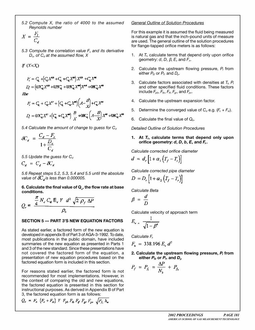
5.2 Compute X, the ratio of 4000 to the assumedReynolds number
5.3 Compute the correlation value Fc and its derivativeDc, of Cd at the assumed flow, X
5.4 Calculate the amount of change to guess for Cd
5.5 Update the guess for Cd
5.6 Repeat steps 5.2, 5.3, 5.4 and 5.5 until the absolutevalue of is less than 0.000005.
6. Calculate the final value of Qv, the flow rate at baseconditions.
SECTION 5 — PART 3’S NEW EQUATION FACTORS
As stated earlier, a factored form of the new equation isdeveloped in appendix B of Part 3 of AGA-3-1992. To date,most publications in the public domain, have includedsummaries of the new equation as presented in Parts 1and 3 of the new standard. Since these presentations havenot covered the factored form of the equation, apresentation of new equation procedures based on thefactored equation form is included in this section.
For reasons stated earlier, the factored form is notrecommended for most implementations. However, inthe context of comparing the old and new equations,the factored equation is presented in this section forinstructional purposes. As derived in Appendix B of Part3, the factored equation form is as follows:
General Outline of Solution Procedures
For this example it is assumed the fluid being measuredis natural gas and that the inch-pound units of measureare used. The general outline of the solution proceduresfor flange-tapped orifice meters is as follows:
1. At Tf, calculate terms that depend only upon orificegeometry: d, D, β, Ev and Fn.
2. Calculate the upstream flowing pressure, Pf fromeither Pf2 or Pf1 and Dp.
3. Calculate factors associated with densities at Tf, Pf
and other specified fluid conditions. These factorsinclude Fpb, Ftb, Ftf, Fgr, and Fpv.
4. Calculate the upstream expansion factor.
5. Determine the converged value of Cd e.g. (Fc + Fsl).
6. Calculate the final value of Qb.
Detailed Outline of Solution Procedures
1. At Tf, calculate terms that depend only uponorifice geometry: d, D, b, Ev and Fn.
Calculate corrected orifice diameter
Calculate corrected pipe diameter
Calculate Beta
Calculate velocity of approach term
Calculate Fn
2. Calculate the upstream flowing pressure, Pf fromeither Pf2 or Pf1 and Dp
PAGE 182 2002 PROCEEDINGSAMERICAN SCHOOL OF GAS MEASUREMENT TECHNOLOGY
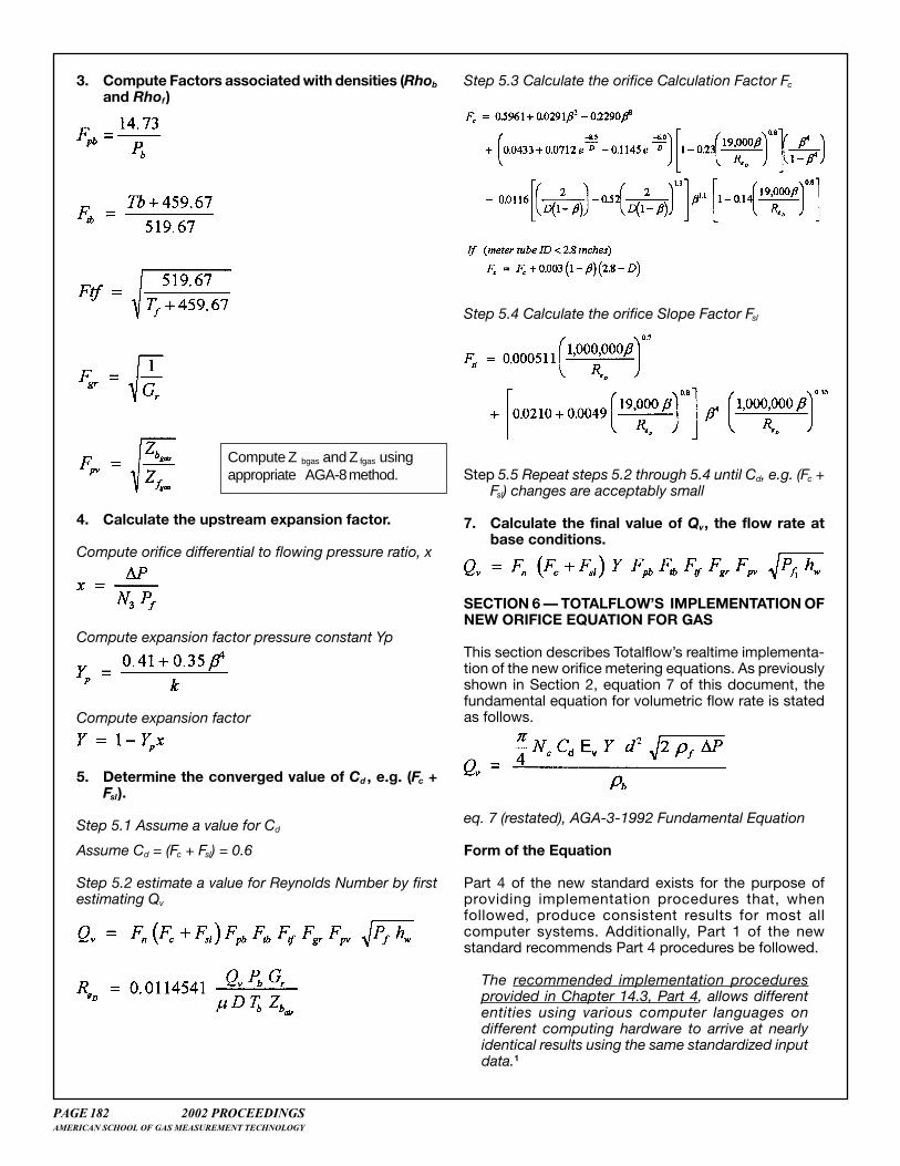
3. Compute Factors associated with densities (Rhob
and Rhof)
4. Calculate the upstream expansion factor.
Compute orifice differential to flowing pressure ratio, x
Compute expansion factor pressure constant Yp
Compute expansion factor
5. Determine the converged value of Cd , e.g. (Fc +Fsl).
Step 5.1 Assume a value for Cd
Assume Cd = (Fc + Fsl) = 0.6
Step 5.2 estimate a value for Reynolds Number by firstestimating Qv
Step 5.3 Calculate the orifice Calculation Factor Fc
Step 5.4 Calculate the orifice Slope Factor Fsl
Step 5.5 Repeat steps 5.2 through 5.4 until Cd, e.g. (Fc +Fsl) changes are acceptably small
7. Calculate the final value of Qv, the flow rate atbase conditions.
SECTION 6 — TOTALFLOW’S IMPLEMENTATION OFNEW ORIFICE EQUATION FOR GAS
This section describes Totalflow’s realtime implementa-tion of the new orifice metering equations. As previouslyshown in Section 2, equation 7 of this document, thefundamental equation for volumetric flow rate is statedas follows.
eq. 7 (restated), AGA-3-1992 Fundamental Equation
Form of the Equation
Part 4 of the new standard exists for the purpose ofproviding implementation procedures that, whenfollowed, produce consistent results for most allcomputer systems. Additionally, Part 1 of the newstandard recommends Part 4 procedures be followed.
The recommended implementation proceduresprovided in Chapter 14.3, Part 4, allows differententities using various computer languages ondifferent computing hardware to arrive at nearlyidentical results using the same standardized inputdata.1
Compute Z bgas and Z fgas usingappropriate AGA-8 method.
2002 PROCEEDINGS PAGE 183AMERICAN SCHOOL OF GAS MEASUREMENT TECHNOLOGY
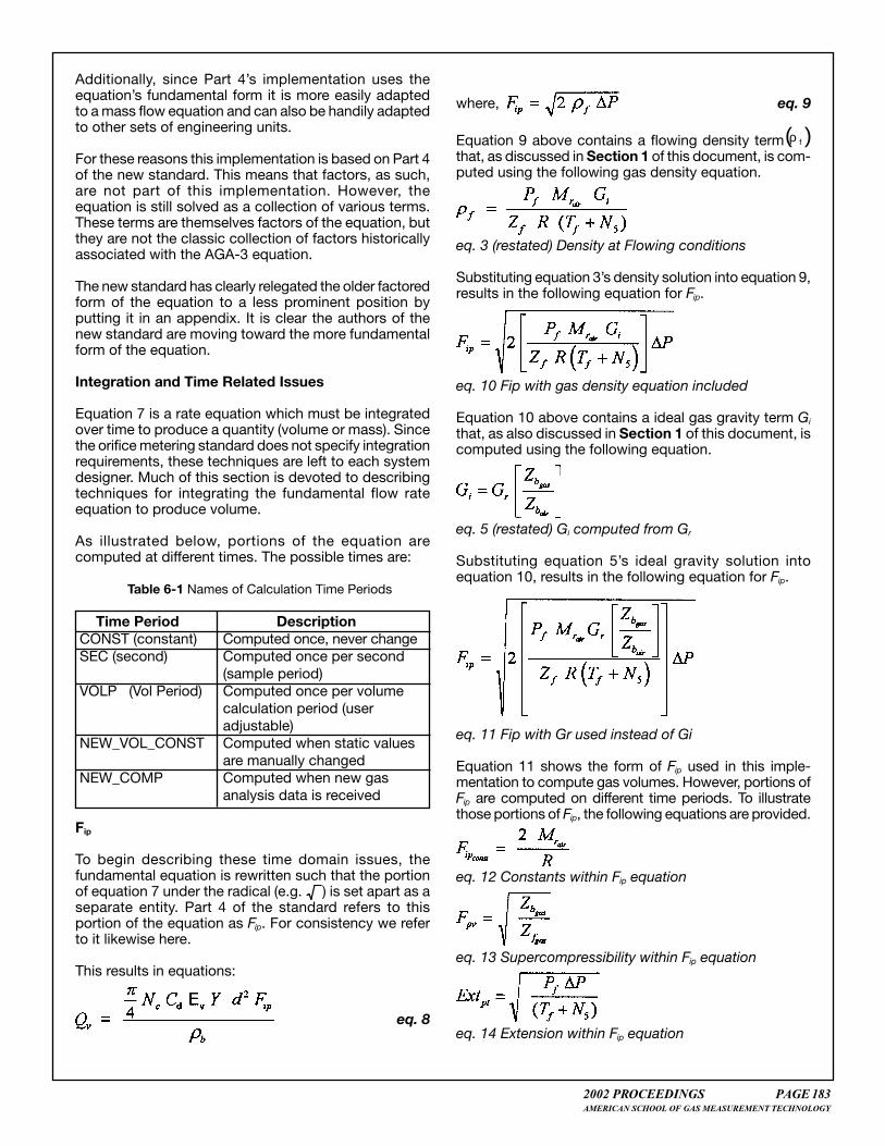
Additionally, since Part 4’s implementation uses theequation’s fundamental form it is more easily adaptedto a mass flow equation and can also be handily adaptedto other sets of engineering units.
For these reasons this implementation is based on Part 4of the new standard. This means that factors, as such,are not part of this implementation. However, theequation is still solved as a collection of various terms.These terms are themselves factors of the equation, butthey are not the classic collection of factors historicallyassociated with the AGA-3 equation.
The new standard has clearly relegated the older factoredform of the equation to a less prominent position byputting it in an appendix. It is clear the authors of thenew standard are moving toward the more fundamentalform of the equation.
Integration and Time Related Issues
Equation 7 is a rate equation which must be integratedover time to produce a quantity (volume or mass). Sincethe orifice metering standard does not specify integrationrequirements, these techniques are left to each systemdesigner. Much of this section is devoted to describingtechniques for integrating the fundamental flow rateequation to produce volume.
As illustrated below, portions of the equation arecomputed at different times. The possible times are:
Table 6-1 Names of Calculation Time Periods
Time Period DescriptionCONST (constant) Computed once, never changeSEC (second) Computed once per second
(sample period)VOLP (Vol Period) Computed once per volume
calculation period (useradjustable)
NEW_VOL_CONST Computed when static valuesare manually changed
NEW_COMP Computed when new gasanalysis data is received
Fip
To begin describing these time domain issues, thefundamental equation is rewritten such that the portionof equation 7 under the radical (e.g. ) is set apart as aseparate entity. Part 4 of the standard refers to thisportion of the equation as Fip. For consistency we referto it likewise here.
This results in equations:
eq. 8
where, eq. 9
Equation 9 above contains a flowing density term( )ρ f
that, as discussed in Section 1 of this document, is com-puted using the following gas density equation.
eq. 3 (restated) Density at Flowing conditions
Substituting equation 3’s density solution into equation 9,results in the following equation for Fip.
eq. 10 Fip with gas density equation included
Equation 10 above contains a ideal gas gravity term Gi
that, as also discussed in Section 1 of this document, iscomputed using the following equation.
eq. 5 (restated) Gi computed from Gr
Substituting equation 5’s ideal gravity solution intoequation 10, results in the following equation for Fip.
eq. 11 Fip with Gr used instead of Gi
Equation 11 shows the form of Fip used in this imple-mentation to compute gas volumes. However, portions ofFip are computed on different time periods. To illustratethose portions of Fip, the following equations are provided.
eq. 12 Constants within Fip equation
eq. 13 Supercompressibility within Fip equation
eq. 14 Extension within Fip equation
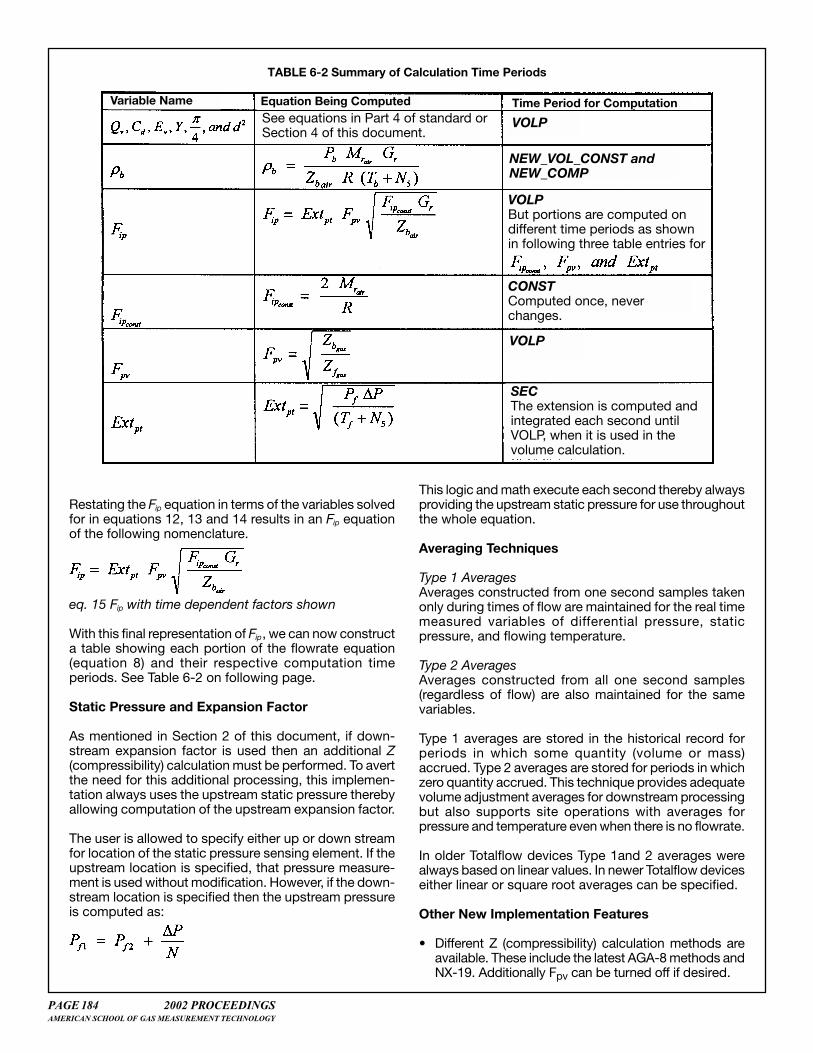
PAGE 184 2002 PROCEEDINGSAMERICAN SCHOOL OF GAS MEASUREMENT TECHNOLOGY
Restating the Fip equation in terms of the variables solvedfor in equations 12, 13 and 14 results in an Fip equationof the following nomenclature.
eq. 15 Fip with time dependent factors shown
With this final representation of Fip, we can now constructa table showing each portion of the flowrate equation(equation 8) and their respective computation timeperiods. See Table 6-2 on following page.
Static Pressure and Expansion Factor
As mentioned in Section 2 of this document, if down-stream expansion factor is used then an additional Z(compressibility) calculation must be performed. To avertthe need for this additional processing, this implemen-tation always uses the upstream static pressure therebyallowing computation of the upstream expansion factor.
The user is allowed to specify either up or down streamfor location of the static pressure sensing element. If theupstream location is specified, that pressure measure-ment is used without modification. However, if the down-stream location is specified then the upstream pressureis computed as:
This logic and math execute each second thereby alwaysproviding the upstream static pressure for use throughoutthe whole equation.
Averaging Techniques
Type 1 AveragesAverages constructed from one second samples takenonly during times of flow are maintained for the real timemeasured variables of differential pressure, staticpressure, and flowing temperature.
Type 2 AveragesAverages constructed from all one second samples(regardless of flow) are also maintained for the samevariables.
Type 1 averages are stored in the historical record forperiods in which some quantity (volume or mass)accrued. Type 2 averages are stored for periods in whichzero quantity accrued. This technique provides adequatevolume adjustment averages for downstream processingbut also supports site operations with averages forpressure and temperature even when there is no flowrate.
In older Totalflow devices Type 1and 2 averages werealways based on linear values. In newer Totalflow deviceseither linear or square root averages can be specified.
Other New Implementation Features
• Different Z (compressibility) calculation methods areavailable. These include the latest AGA-8 methods andNX-19. Additionally Fpv can be turned off if desired.
TABLE 6-2 Summary of Calculation Time Periods
SECThe extension is computed andintegrated each second untilVOLP, when it is used in thevolume calculation.
VOLP
CONSTComputed once, neverchanges.
VOLPBut portions are computed ondifferent time periods as shownin following three table entries for
NEW_VOL_CONST andNEW_COMP
VOLPSee equations in Part 4 of standard orSection 4 of this document.
Time Period for ComputationEquation Being ComputedVariable Name
2002 PROCEEDINGS PAGE 185AMERICAN SCHOOL OF GAS MEASUREMENT TECHNOLOGY
• VOLP, Volume calculation period defaults to one hour,but is user selectable. Selections offered are 1, 2, 5,10, 30, and 60 minutes.
• Up to 23 composition variables for supporting AGA-8detailed method are supported.
• Selectable static pressure tap location is supported.
• Selectable differential pressure tap type is supported.
• Higher static pressure transducers are supported. Upto 3500 psi is currently in use.
Algorithmic Detail of Realtime Implementation of NewEquation for Gas
The following is a more detailed summary of periodiccomputations performed by this implementation forsolving the new orifice equations (AGA-3-1992). Theperiods referred to in this section are those same periodssummarized in Table 6-1. Please note that the followingequations are based on using linear averages, if squareroot averages are selected, then square roots areperformed before they one second summations takeplace.
CONST PERIOD
NEW COMP PERIOD & NEW VOL CONSTS PERIOD
Currently the same calculations are being performed foreach of these two periods. Future optimizations couldresult in different calculations being performed for eachof these two periods.
Perform Fpv Pre-Calculations
IF (Fpv Method = AGA-8 gross)Compute AGA-8 gross method precalcs (e.g. AGA-8 terms that are function of composition) UsingAGA-8 gross method Compute Zbgas
ELSE IF (Fpv Method = AGA-8detail)Compute AGA-8 detail method precalcs (e.g. AGA-8 terms that are function of composition) UsingAGA-8 detail method Compute Zbgas
ELSE IF (Fpv Method = NX19_FIXEDFTFP)Accept user supplied Ft and Fp values
ELSE IF (Fpv Method = NX19)
IF ((Gr < 0.75) AND (CO2 < 15%) AND (N2 < 15%))Compute Ft and Fp using NX19 Gravity Method
ELSECompute Ft and Fp using Methane Gravity MethodENDIF
Fip
Fipconst
ELSE IF (Fpv Method = NX19_GRAVITY)Compute Ft and Fp using NX19 Gravity Method
ELSE IF (Fpv Method = NX19_METHANE-GRAVITY)Compute Ft and Fp using NX19 Methane GravityMethod
ENDIF
Calculate Base Density
SEC PERIOD
IF (Pressure Tap Downstream)Calculated Upstream Static Pressure, Pf
IF (DP > DP_ZERO_CUTOFF) (If Flow Exists)
ENDIF
VOLP (VOL PERIOD)(THIS ONLY EXECUTES IF THERE WAS FLOWDURING THE VOLP)
ELSE
ENDIF
PAGE 186 2002 PROCEEDINGSAMERICAN SCHOOL OF GAS MEASUREMENT TECHNOLOGY
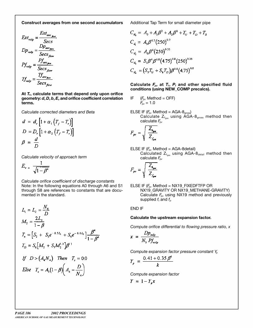
Construct averages from one second accumulators
At Tf, calculate terms that depend only upon orificegeometry: d, D, b, Ev and orifice coefficient correlationterms.
Calculate corrected diameters and Beta
Calculate velocity of approach term
Calculate orifice coefficient of discharge constantsNote: In the following equations A0 through A6 and S1through S8 are references to constants that are docu-mented in the standard.
Additional Tap Term for small diameter pipe
Calculate Fpv at Tf , Pf and other specified fluidconditions (using NEW_COMP precalcs).
IF (Fpv Method = OFF)Fpv = 1.0
ELSE IF (Fpv Method = AGA-8gross)Calculate Zfgas using AGA-8gross method thencalculate Fpv
ELSE IF (Fpv Method = AGA-8detail)Calculated Zfgas using AGA-8detail method thencalculate Fpv
ELSE IF (Fpv Method = NX19_FIXEDFTFP ORNX19_GRAVITY OR NX19_METHANE-GRAVITY)Calculate Fpv using NX19 method and previouslysupplied ft and fp
END IF
Calculate the upstream expansion factor.
Compute orifice differential to flowing pressure ratio, x
Compute expansion factor pressure constant Yp
Compute expansion factor
2002 PROCEEDINGS PAGE 187AMERICAN SCHOOL OF GAS MEASUREMENT TECHNOLOGY
Calculate Fip
Determine the converged value of Cd.
Cd_step.0 Calculate the iteration flow factor, Fi, andits component part, Fip. Re-use the Fip com-puted earlier. Then use these in the Cd con-vergence scheme.
Compute Cd’s Iteration flow factor, FI
If Fic < 1000 Fip
Cd_step.1 Initialize Cd to value at infinite Reynoldsnumber
Cd_step.2 Compute X, the ratio of 4000 to the
assumed Reynolds number
Cd_step.3 Compute the correlation value Fc and it’sderivative Dc, of Cd at the assumed flow, X
Cd_step.4 Calculate the amount of change to guessfor Cd
Cd_step.5 Update the guess for Cd
Cd_step.6 Repeat steps 2,3,4 and 5 until the absolutevalue of is less than 0.000005.
Calculate the final value of qm , the mass flow rate atline conditions.
Calculate the final value of Qv , the volumetric flowrate at base conditions.
Calculate the final value of Volb , the volume at baseconditions for the Volume Period
Section 7 - NOMENCLATURE
a1 Linear coefficient of thermal expansion of theorifice plate material
a2 Linear coefficient of thermal expansion of themeter tube material.
b Beta. Ratio of orifice plate bore diameter to metertube internal diameter (d/D) at flowing tempera-ture,Tf.
Cd Orifice plate coefficient of discharge.
Cd0 First flange-tapped orifice plate coefficient ofdischarge constant within iteration scheme.
Cd1 Second flange-tapped orifice plate coefficientof discharge constant within iteration scheme.
Cd2 Third flange-tapped orifice plate coefficient ofdischarge constant within iteration scheme.
Cd3 Forth flange-tapped orifice plate coefficient ofdischarge constant within iteration scheme.
Cd4 Fifth flange-tapped orifice plate coefficient ofdischarge constant within iteration scheme.
Cd_f Orifice plate coefficient of discharge bounds flagwithin iteration scheme.
d Orifice plate bore diameter calculated at flowingtemperature Tt.
D Meter tube internal diameter calculated atflowing temperature Tf.
dr Orifice plate bore diameter calculated atreference temperature Tr.
Dr Meter tube internal diameter calculated atreference temperature Tr.
V
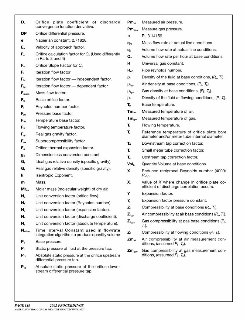
PAGE 188 2002 PROCEEDINGSAMERICAN SCHOOL OF GAS MEASUREMENT TECHNOLOGY
Dc Orifice plate coefficient of dischargeconvergence function derivative.
DP Orifice differential pressure.
e Napierian constant, 2.71828.
Ev Velocity of approach factor.
Fc Orifice calculation factor for Cd (Used differentlyin Parts 3 and 4)
Fsl Orifice Slope Factor for Cd
Fl Iteration flow factor
Flc Iteration flow factor — independent factor.
Flp Iteration flow factor — dependent factor.
Fmass Mass flow factor.
Fb Basic orifice factor.
Fr Reynolds number factor.
Fpb Pressure base factor.
Ftb Temperature base factor.
Ftf Flowing temperature factor.
Fgr Real gas gravity factor.
Fpv Supercompressibility factor.
Fa Orifice thermal expansion factor.
gc Dimensionless conversion constant.
Gi Ideal gas relative density (specific gravity).
Gr Real gas relative density (specific gravity).
k Isentropic Exponent.
m Mass.
Mrair Molar mass (molecular weight) of dry air.
Nc Unit conversion factor (orifice flow).
N1 Unit conversion factor (Reynolds number).
N3 Unit conversion factor (expansion factor).
N4 Unit conversion factor (discharge coefficient).
N5 Unit conversion factor (absolute temperature).
Nvtime Time Interval Constant used in flowrateintegration algorithm to produce quantity volume
Pb Base pressure.
Pf Static pressure of fluid at the pressure tap.
Pf1 Absolute static pressure at the orifice upstreamdifferential pressure tap.
Pf2 Absolute static pressure at the orifice down-stream differential pressure tap.
Pmair Measured air pressure.
Pmgas Measure gas pressure.
π Pi, 3.14159
qm Mass flow rate at actual line conditions
qv Volume flow rate at actual line conditions.
Qv Volume flow rate per hour at base conditions.
R Universal gas constant.
ReD Pipe reynolds number.
ρb Density of the fluid at base conditions, (Pb, Tb).
ρbair Air density at base conditions, (Pb, Tb).
ρbgas Gas density at base conditions, (Pb, Tb).
ρf Density of the fluid at flowing conditions, (Pf, Tf).
Tb Base temperature.
Tmair Measured temperature of air.
Tmgas Measured temperature of gas.
Tf Flowing temperature.
Tr Reference temperature of orifice plate borediameter and/or meter tube internal diameter.
Td Downstream tap correction factor.
Ts Small meter tube correction factor.
Tu Upstream tap correction factor.
Volb Quantity Volume at base conditions
X Reduced reciprocal Reynolds number (4000/ReD).
Xc Value of X where change in orifice plate co-efficient of discharge correlation occurs.
Y Expansion factor.
Yp Expansion factor pressure constant.
Zb Compressibility at base conditions (Pb, Tb).
Zbair Air compressibility at air base conditions (Pb, Tb).
Zbgas Gas compressibility at gas base conditions (Pb,Tb).
Zf Compressibility at flowing conditions (Pf, Tf).
Zmair Air compressibility at air measurement con-ditions, (assumed Pb, Tb).
Zmgas Gas compressibility at gas measurement con-ditions, (assumed Pb, Tb).
2002 PROCEEDINGS PAGE 189AMERICAN SCHOOL OF GAS MEASUREMENT TECHNOLOGY
Section 8 — CITED PUBLICATIONS
1. American Petroleum Institute Measurement onPetroleum Measurement Standards (API MPMS)Chapter 14.3, Part 1; Also recognized as AGA ReportNo. 3 Part 1; Also recognized as GPA 8185-92, Part3; Also recognized as ANSI/API 2530-1991, Part 1
2. American Petroleum Institute Measurement onPetroleum Measurement Standards (API MPMS)Chapter 14.3, Part 2; Also recognized as AGA ReportNo. 3 Part 2; Also recognized as GPA 8185-92, Part2; Also recognized as ANSI/API 2530-1991, Part 2
3. American Petroleum Institute Measurement onPetroleum Measurement Standards (API MPMS)Chapter 14.3, Part 3; Also recognized as AGA ReportNo. 3 Part 3; Also recognized as GPA 8185-92, Part3; Also recognized as ANSI/API 2530-1991, Part 3
4. American Petroleum Institute Measurement onPetroleum Measurement Standards (API MPMS)Chapter 14.3, Part 4; Also recognized as AGA ReportNo. 3 Part 4; Also recognized as GPA 8185-92, Part4; Also recognized as ANSI/API 2530-1991, Part 4
5. American Gas Association (AGA) TransmissionMeasurement Committee Report No. 8; Alsorecognized as API MPMS Chapter 14.2.
6. Teyssandier, Raymond G.; Beaty, Ronald: New orificemeter standards improve gas calculations, Oil & GasJournal, Jan. 11, 1993
7. ANSI/API 2530: Second Edition, 1985, OrificeMetering Of Natural Gas and Other RelatedHydrocarbon Fluids; Also recognized as AGA ReportNo. 3; Also recognized as GPA 8185-85; Alsorecognized as API MPMS Chapter 14.3, API 2530.
Brent E. Berry