Adversarial Search (a.k.a. Game Playing)

C h a p t e r 5

(AdaptedfromStuartRussell,DanKlein,andothers.Thanksguys!)

Outline

•  Games

•  Perfect play: principles of adversarial search

–  minimax decisions

–  α–β pruning

–  Move ordering

•  Imperfect play: dealing with resource limits

–  Cutting of search and approximate evaluation

•  Stochastic games (games of chance)

•  Partially Observable games

•  Card Games

2

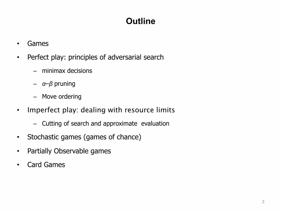
Games vs. search problems

•  Search in Ch3&4: Single actor! –  “single player” scenario or game, e.g., Boggle. –  Brain teasers: one player against “the game”. –  Could be adversarial, but not directly as part of game

•  e.g. “I can find more words than you”

•  Adversarial game: “Unpredictable” opponent shares control of state –  solution is a strategy à specifying a move for every possible opponent

response –  Time limits ⇒ unlikely to find goal, must find optimal move with incomplete

search –  Major penalty for inefficiency (you get your clock cleaned) –  Most commonly: “zero-sum” games. My gain is your loss = Adversarial

•  Gaming has a deep history in computational thinking –  Computer considers possible lines of play (Babbage, 1846) –  Algorithm for perfect play (Zermelo, 1912; Von Neumann, 1944) –  Finite horizon, approximate evaluation (Zuse, 1945; Wiener, 1948; Shannon, 1950) –  First chess program (Turing, 1951) –  Machine learning to improve evaluation accuracy (Samuel, 1952–57) –  Pruning to allow deeper search (McCarthy, 1956) –  Plus explosion of more modern results...

3

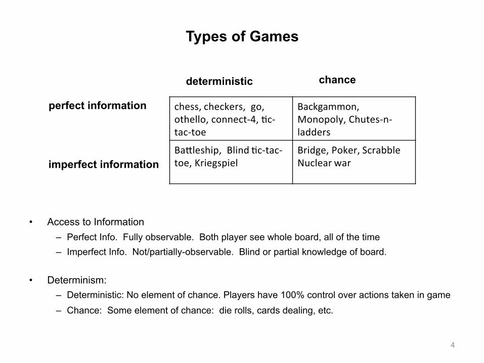
Types of Games

•  Access to Information –  Perfect Info. Fully observable. Both player see whole board, all of the time –  Imperfect Info. Not/partially-observable. Blind or partial knowledge of board.

•  Determinism: –  Deterministic: No element of chance. Players have 100% control over actions taken in game –  Chance: Some element of chance: die rolls, cards dealing, etc.

4

deterministic chance

perfect information

imperfect information

chess,checkers,go,othello,connect-4,Dc-tac-toe

Backgammon,Monopoly,Chutes-n-ladders

BaHleship,BlindDc-tac-toe,Kriegspiel

Bridge,Poker,ScrabbleNuclearwar

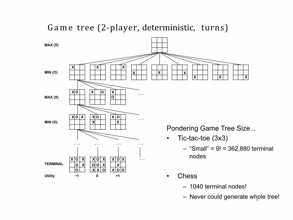
Game tree(2-player,deterministic,turns)

X X X X

X X

X X

MAX (X)

MIN (O)

X O

X O MAX (X)

X O X

X O X MIN (O)

X

X O

X O X

. . . . . . . . . . . .

. . .

. . .

X O X O X O

. . . TERMINAL

−1 0 +1 Utility

X O X O O X X X O

X O X X

X O O

5

Pondering Game Tree Size... •  Tic-tac-toe (3x3)

–  “Small” = 9! = 362,880 terminal nodes

•  Chess –  1040 terminal nodes!

–  Never could generate whole tree!

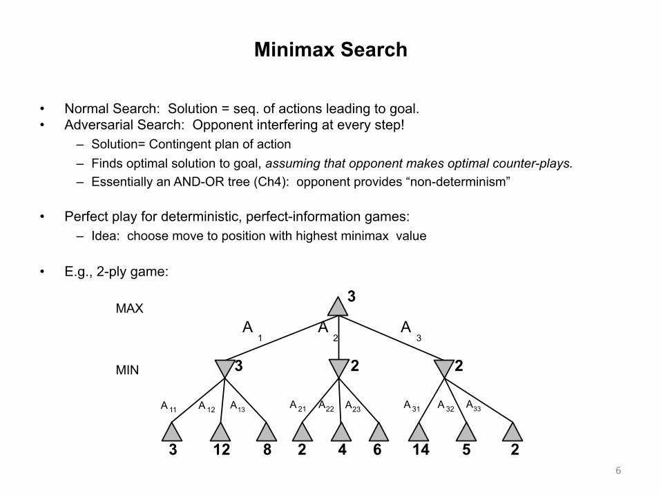
Minimax Search

6

MAX

3 12 4 6 8 2 14 5 2

MIN

A 1

A 3

A 2

A 11 A 12 A 13 A 23 A 21 A 22 A 31 A 32 A 33

3 2 2

3

•  Normal Search: Solution = seq. of actions leading to goal. •  Adversarial Search: Opponent interfering at every step!

–  Solution= Contingent plan of action –  Finds optimal solution to goal, assuming that opponent makes optimal counter-plays. –  Essentially an AND-OR tree (Ch4): opponent provides “non-determinism”

•  Perfect play for deterministic, perfect-information games: –  Idea: choose move to position with highest minimax value

•  E.g., 2-ply game:

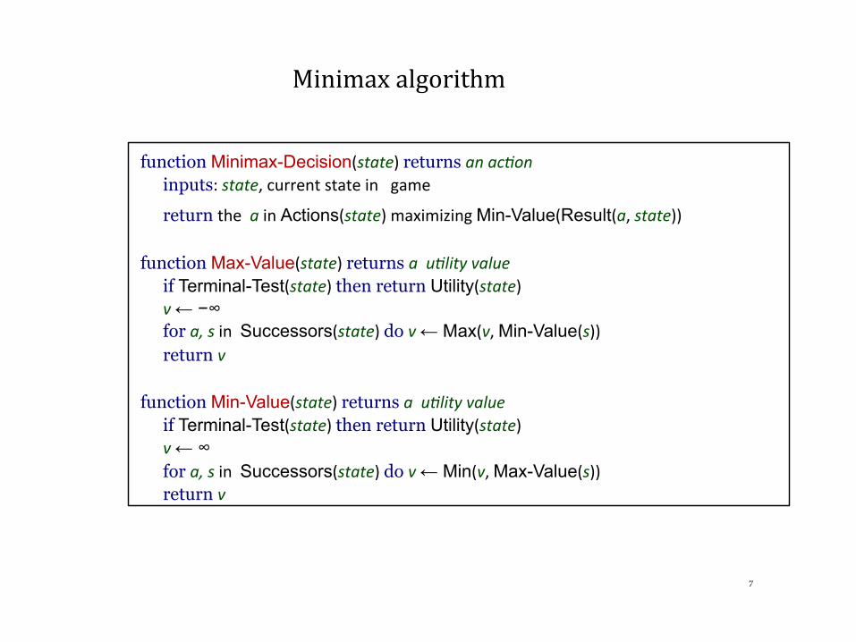
Minimaxalgorithm

function Minimax-Decision(state)returns anac(oninputs:state,currentstateingame

return theainActions(state)maximizingMin-Value(Result(a,state))

function Max-Value(state)returns au(lityvalueif Terminal-Test(state)then return Utility(state)v← −∞ for a,sinSuccessors(state)do v← Max(v,Min-Value(s))return v

function Min-Value(state)returns au(lityvalue

if Terminal-Test(state)then return Utility(state)v← ∞ for a,sinSuccessors(state)do v← Min(v,Max-Value(s))return v

7

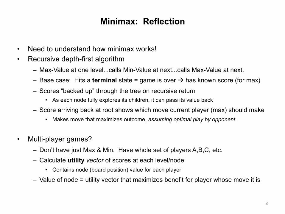
Minimax: Reflection

•  Need to understand how minimax works! •  Recursive depth-first algorithm

–  Max-Value at one level...calls Min-Value at next...calls Max-Value at next. –  Base case: Hits a terminal state = game is over à has known score (for max)

–  Scores “backed up” through the tree on recursive return •  As each node fully explores its children, it can pass its value back

–  Score arriving back at root shows which move current player (max) should make •  Makes move that maximizes outcome, assuming optimal play by opponent.

•  Multi-player games? –  Don’t have just Max & Min. Have whole set of players A,B,C, etc. –  Calculate utility vector of scores at each level/node

•  Contains node (board position) value for each player

–  Value of node = utility vector that maximizes benefit for player whose move it is

8

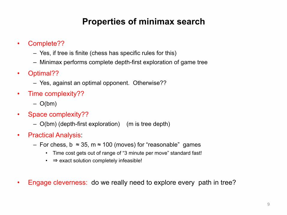
Properties of minimax search

•  Complete?? –  Yes, if tree is finite (chess has specific rules for this) –  Minimax performs complete depth-first exploration of game tree

•  Optimal?? –  Yes, against an optimal opponent. Otherwise??

•  Time complexity?? –  O(bm)

•  Space complexity?? –  O(bm) (depth-first exploration) (m is tree depth)

•  Practical Analysis: –  For chess, b ≈ 35, m ≈ 100 (moves) for “reasonable” games

•  Time cost gets out of range of “3 minute per move” standard fast! •  ⇒ exact solution completely infeasible!

•  Engage cleverness: do we really need to explore every path in tree?

9

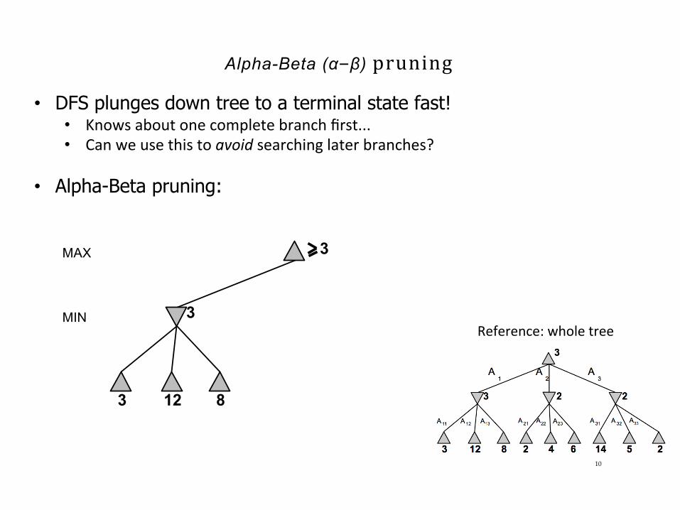
Alpha-Beta (α–β) pruning

MAX

3 12 8

MIN 3

3

10

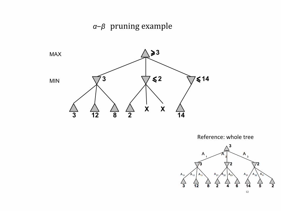
Reference:wholetree

•  DFS plunges down tree to a terminal state fast! •  Knowsaboutonecompletebranchfirst...•  Canweusethistoavoidsearchinglaterbranches?

•  Alpha-Beta pruning:

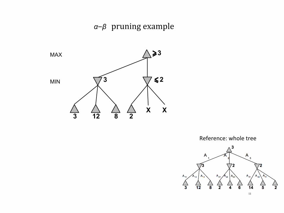
α–β pruningexample

MAX

3 12

MIN 3

8 2

2

X X

3

11

Reference:wholetree

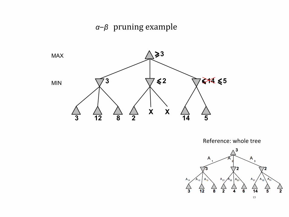
α–β pruningexample

MAX

3 12

MIN 3

8 2

2

X X 14

14

3

12

Reference:wholetree

α–β pruningexample

MAX

3 12

MIN 3

8 2

2

X X 14 5

14 5

3

13

Reference:wholetree

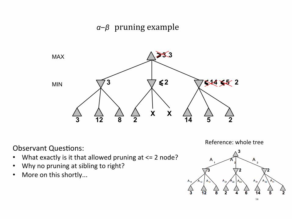
α–β pruningexample

MAX

3 12

MIN 3

8 2

2

X X 14 5 2

14 5 2

3 3

14

Reference:wholetreeObservantQuesDons:•  Whatexactlyisitthatallowedpruningat<=2node?•  Whynopruningatsiblingtoright?•  Moreonthisshortly...

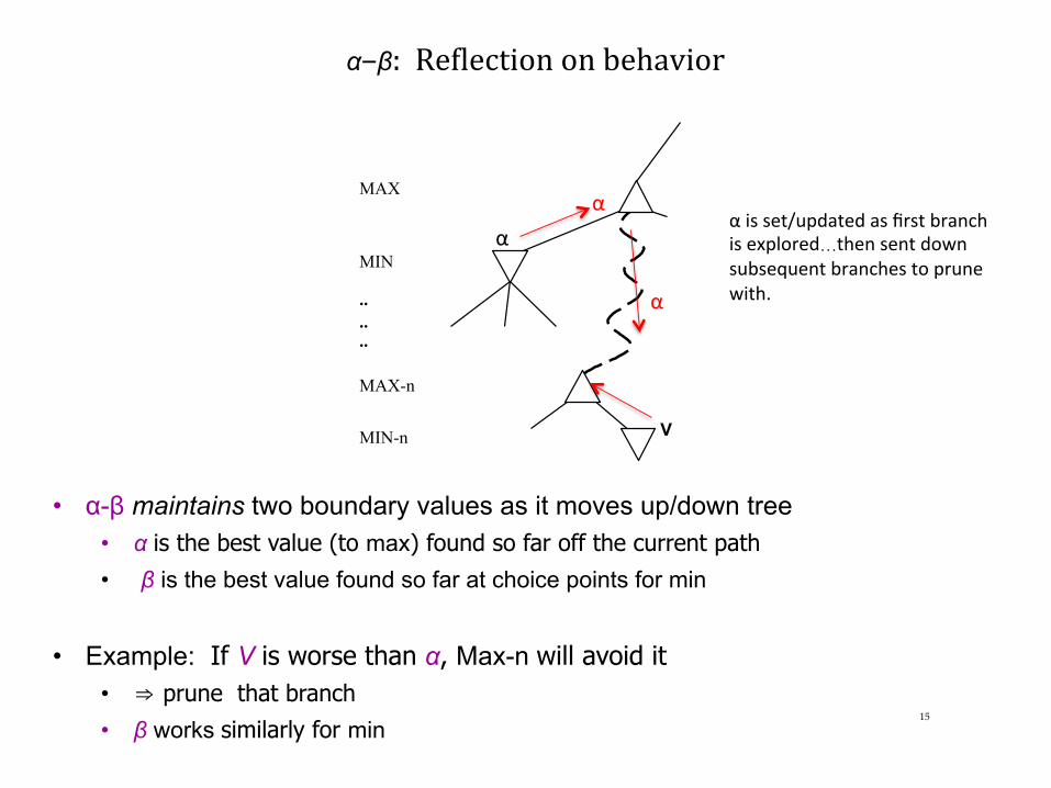
α–β:Re>lectiononbehavior

15

•  α-β maintains two boundary values as it moves up/down tree •  α is the best value (to max) found so far off the current path •  β is the best value found so far at choice points for min

•  Example: If V is worse than α, Max-n will avoid it •  ⇒ prune that branch

•  β works similarly for min

MAX

MIN .. .. .. MAX-n

MIN-n V

αα

α

αisset/updatedasfirstbranchisexplored…thensentdownsubsequentbranchestoprunewith.

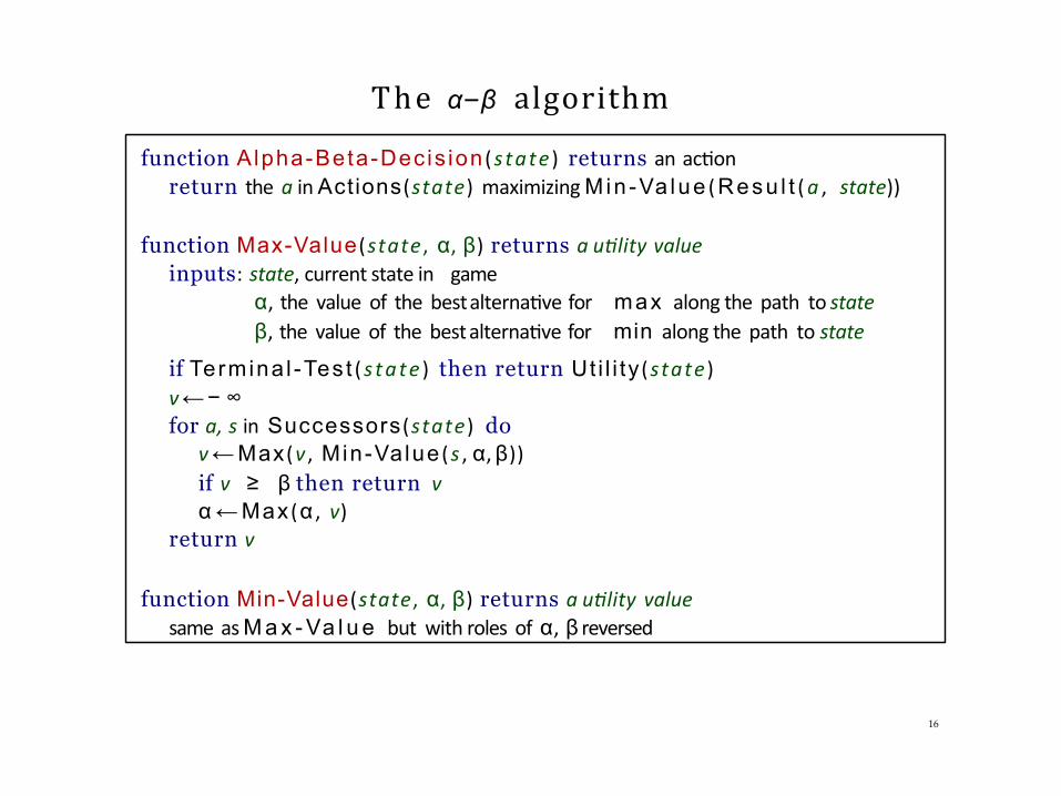
The α–β algorithm

function Alpha-Beta-Decis ion (s tate ) returns anacDonreturn theainActions(state) maximizingMin-Va lue (Resu l t (a , state))

function Max-Value(state , α,β)returns au(lityvalue

inputs:state,currentstatein gameα,thevalueofthebestalternaDvefor max alongthepathtostateβ,thevalueofthebestalternaDvefor min alongthepathtostate

if Termina l -Test ( s ta te ) then return Uti l i ty (state ) v← − ∞ for a,sinSuccessors (state ) do

v← Max (v , Min-Value (s , α,β))if v ≥ β then return vα ← Max (α , v)

return v

function Min-Value(state , α,β)returns au(lityvaluesameasM a x - Va l u e butwithrolesofα,β reversed

16

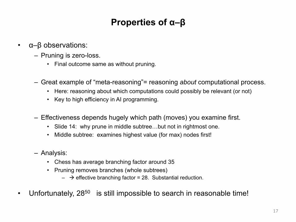
Properties of α–β

•  α–β observations: –  Pruning is zero-loss.

•  Final outcome same as without pruning.

–  Great example of “meta-reasoning”= reasoning about computational process. •  Here: reasoning about which computations could possibly be relevant (or not) •  Key to high efficiency in AI programming.

–  Effectiveness depends hugely which path (moves) you examine first. •  Slide 14: why prune in middle subtree…but not in rightmost one. •  Middle subtree: examines highest value (for max) nodes first!

–  Analysis: •  Chess has average branching factor around 35 •  Pruning removes branches (whole subtrees)

–  à effective branching factor = 28. Substantial reduction.

•  Unfortunately, 2850 is still impossible to search in reasonable time!

17

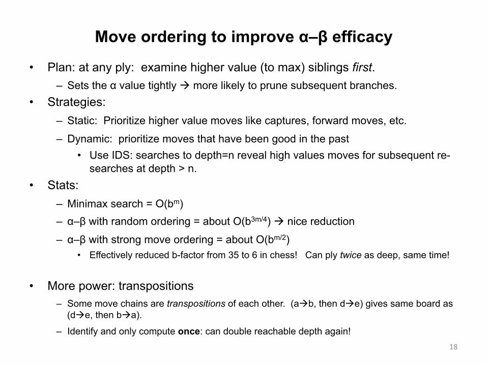
Move ordering to improve α–β efficacy

•  Plan: at any ply: examine higher value (to max) siblings first. –  Sets the α value tightly à more likely to prune subsequent branches.

•  Strategies: –  Static: Prioritize higher value moves like captures, forward moves, etc.

–  Dynamic: prioritize moves that have been good in the past •  Use IDS: searches to depth=n reveal high values moves for subsequent re-

searches at depth > n. •  Stats:

–  Minimax search = O(bm) –  α–β with random ordering = about O(b3m/4) à nice reduction

–  α–β with strong move ordering = about O(bm/2) •  Effectively reduced b-factor from 35 to 6 in chess! Can ply twice as deep, same time!

•  More power: transpositions –  Some move chains are transpositions of each other. (aàb, then dàe) gives same board as

(dàe, then bàa).

–  Identify and only compute once: can double reachable depth again!

18

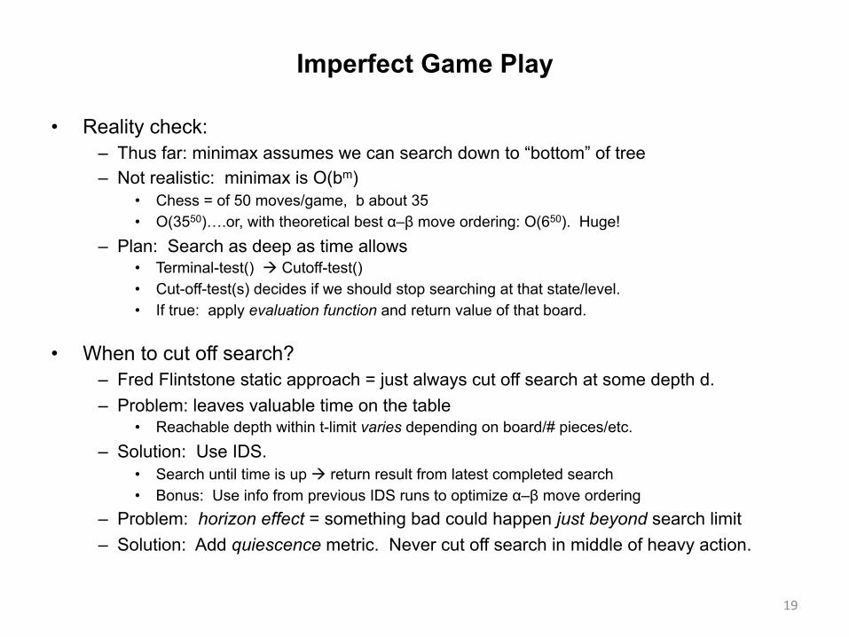
Imperfect Game Play

•  Reality check: –  Thus far: minimax assumes we can search down to “bottom” of tree –  Not realistic: minimax is O(bm)

•  Chess = of 50 moves/game, b about 35 •  O(3550)….or, with theoretical best α–β move ordering: O(650). Huge!

–  Plan: Search as deep as time allows •  Terminal-test() à Cutoff-test() •  Cut-off-test(s) decides if we should stop searching at that state/level. •  If true: apply evaluation function and return value of that board.

•  When to cut off search? –  Fred Flintstone static approach = just always cut off search at some depth d. –  Problem: leaves valuable time on the table

•  Reachable depth within t-limit varies depending on board/# pieces/etc. –  Solution: Use IDS.

•  Search until time is up à return result from latest completed search •  Bonus: Use info from previous IDS runs to optimize α–β move ordering

–  Problem: horizon effect = something bad could happen just beyond search limit –  Solution: Add quiescence metric. Never cut off search in middle of heavy action.

19

Advanced Techniques: when winning matters

•  Idea 1: Find ways to search deeper. –  Efficiency: efficient board representation, faster eval functions, etc. –  Better pruning: maximize efficacy of move ordering subsystem

–  Forward pruning: cut off “un-interesting” branches of search tree early •  α–β prunes nodes that are provably useless à loss-less •  Forward pruning “guesses” à prunes nodes that are probably useless. •  Danger: could prune away moves that ultimately lead to wins! •  Strategy: shallow search gets rough node value. Stored info estimates likely utility

•  Idea 2: More sophisticated evaluation function –  Linear weighted function assume independence of features…statically

•  But often it’s the combo of pieces that count…more at some points in game than others •  E.g., pair of bishops > two bishops…but more so in the end-game •  Non-linear weighted functions allow more subtle tuning

–  Machine learning can also be used to adjust weights from experience

20

Advanced Techniques: when winning matters

•  Idea 3: Avoid search completely when you can

–  In many games, there are certain rote phases •  e.g. Chess: whole libraries of books about standard openings/end games •  Why search down through billions of boards? Look it up!

–  Can just store and look-up moves for “standard” situations •  Enter from books and other “human knowledge” •  Calculate stats on DB of previously played games à which openings won most?

–  Computers can have advantage of humans here! •  Human: has general strategy for certain endgames

–  King-rook-king (KRK) endgame, king-bishop-knight-king (KBNK), etc.

•  Computer: with so few pieces, can literally compute winning move sequence! –  For all possible KRK endings, etc.

•  Computer recognizes a pre-computed sequence à plays perfect deterministic endgame!

21

History: Deterministic Games in practice…

•  Checkers: –  Chinook ended 40-year-reign of human world champion Marion Tinsley in 1994. –  Used an endgame database defining perfect play for all positions involving 8 or fewer

pieces on the board, a total of 443,748,401,247 positions.

•  Chess: –  Deep Blue defeated human world champion Gary Kasparov in a six-game match in

1997. –  Deep Blue searches 200 million positions per second, uses very sophisticated

evaluation, and undisclosed methods for extending some lines of search up to 40 ply.

•  Othello: –  human champions refuse to compete against computers, who are too good.

•  Go: –  2005: human champions refuse to compete against computers, who are too bad. –  In go, b > 300, so most programs use pattern knowledge bases to suggest plausible

moves. –  2017: IBM reveals it has been secretly entering its Go agent in online tournaments.

And winning. Beats reigning Go champion four in a row…

22

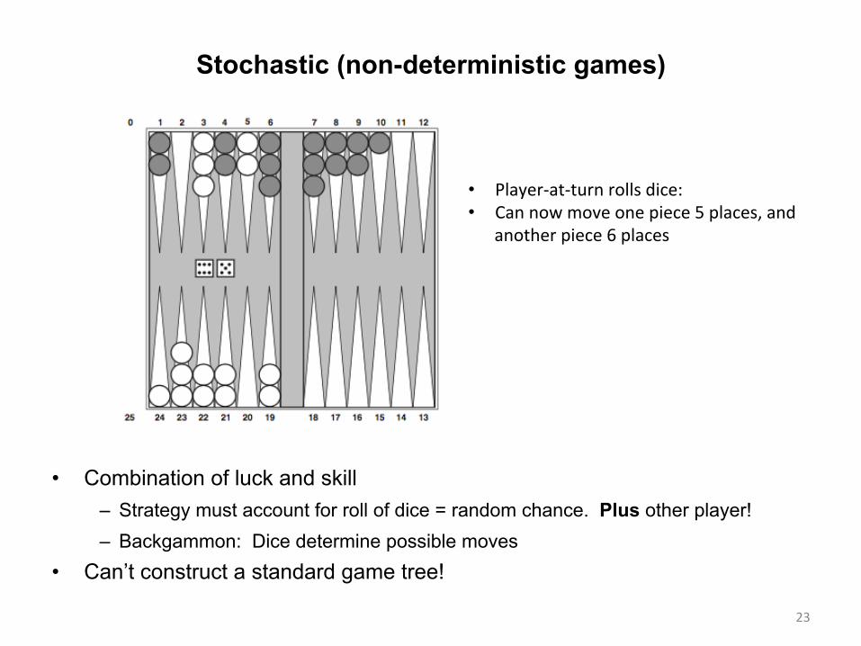
Stochastic (non-deterministic games)

•  Combination of luck and skill –  Strategy must account for roll of dice = random chance. Plus other player! –  Backgammon: Dice determine possible moves

•  Can’t construct a standard game tree!

23

•  Player-at-turnrollsdice:•  Cannowmoveonepiece5places,and

anotherpiece6places

Non-deterministic Games

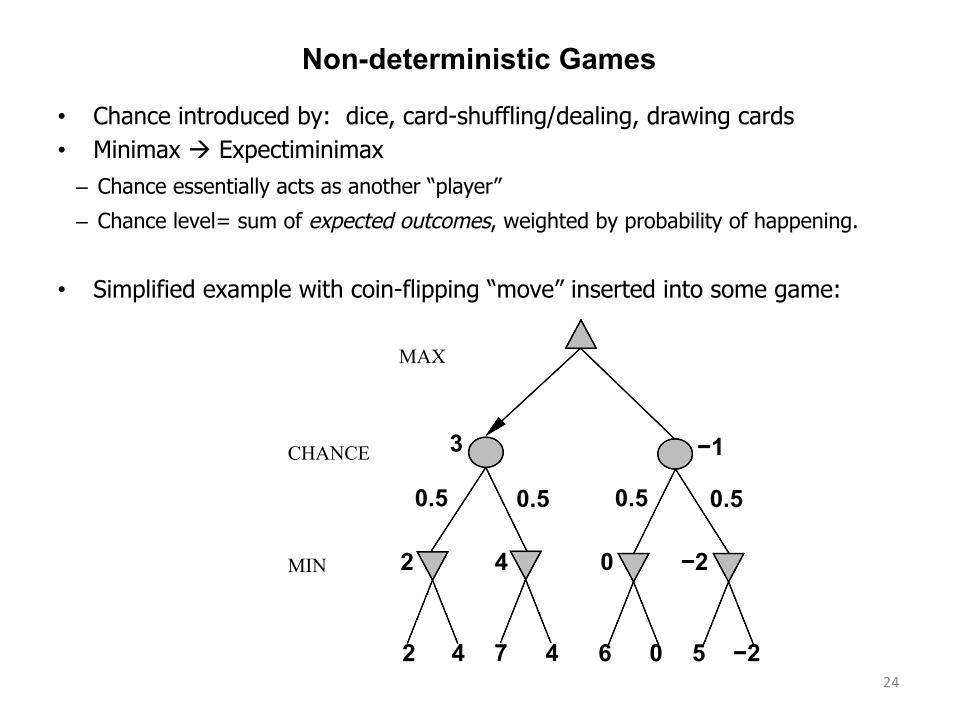
•  Chance introduced by: dice, card-shuffling/dealing, drawing cards •  Minimax à Expectiminimax

–  Chance essentially acts as another “player”

–  Chance level= sum of expected outcomes, weighted by probability of happening.

•  Simplified example with coin-flipping “move” inserted into some game:

24

MIN

CHANCE

2 4 7 4 6 0 5 −2

2 4 0 −2

0.5 0.5 0.5 0.5

3 −1

MAX

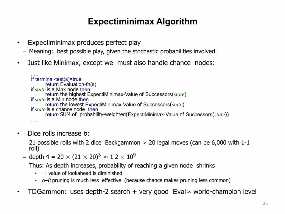
Expectiminimax Algorithm

•  Expectiminimax produces perfect play –  Meaning: best possible play, given the stochastic probabilities involved.

•  Just like Minimax, except we must also handle chance nodes:

. . . If terminal-test(s)=true return Evaluation-fn(s) if stateis a Max node then return the highest ExpectiMinimax-Value of Successors(state) if stateis a Min node then return the lowest ExpectiMinimax-Value of Successors(state) if stateis a chance node then return SUM of probability-weighted(ExpectiMinimax-Value of Successors(state)) . . .

•  Dice rolls increase b: –  21 possible rolls with 2 dice Backgammon ≈ 20 legal moves (can be 6,000 with 1-1

roll) –  depth 4 = 20 × (21 × 20)3 ≈ 1.2 × 109

–  Thus: As depth increases, probability of reaching a given node shrinks •  ⇒ value of lookahead is diminished •  α–β pruning is much less effective (because chance makes pruning less common)

•  TDGammon: uses depth-2 search + very good Eval≈ world-champion level

25

26

Games ofimperfect information

g. ., card games, where opponent’s initial cards are unknown

Typically we can calculate a probability for each possible deal

Seems just like having one big dice roll at the beginning of the game∗ Idea:

compute the minimax value of each action in each deal, then choose the action with highest expected value over all deals∗

Special case: if an action is optimal for all deals, it’s optimal.∗

GIB, current best bridge program, approximates this idea by 1) generating 100 deals consistent with bidding information 2) picking the action that wins most tricks on average

Partially Observable Games

•  So far: Fully observable games –  All player can see all functional pieces (state) of the game at all times

•  Many games are fun because of imperfect information –  Players see only none/part of opponents state. –  E.g. Poker and similar card games, Battleship, etc.

•  Example: Kriegspiel: Blind chess! –  White and Black see only a board containing their pieces. –  On turn: player proposes a move.

•  Referee announced: legal/illegal. If legal: “Capture on square X”, “Check by <direction>”, “checkmate” or “stalemate”.

–  Plan: Use belief states developed in Ch4! •  Referee feedback = percepts that update/prune belief states. •  All believe states NOT equally likely: can calculate probabilities on believe states

based predicting optimum play by opponent. •  Implication: Best to add some randomness to your play: be unpredictable!

27

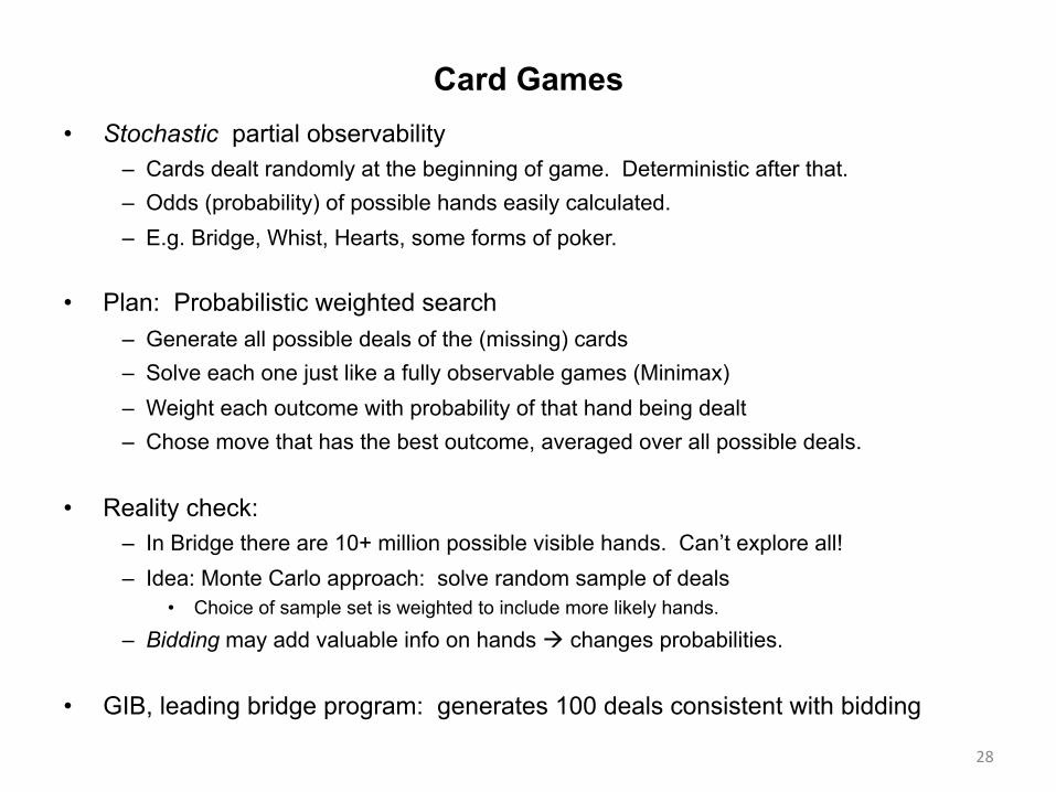
Card Games •  Stochastic partial observability

–  Cards dealt randomly at the beginning of game. Deterministic after that. –  Odds (probability) of possible hands easily calculated. –  E.g. Bridge, Whist, Hearts, some forms of poker.

•  Plan: Probabilistic weighted search –  Generate all possible deals of the (missing) cards –  Solve each one just like a fully observable games (Minimax) –  Weight each outcome with probability of that hand being dealt –  Chose move that has the best outcome, averaged over all possible deals.

•  Reality check: –  In Bridge there are 10+ million possible visible hands. Can’t explore all! –  Idea: Monte Carlo approach: solve random sample of deals

•  Choice of sample set is weighted to include more likely hands.

–  Bidding may add valuable info on hands à changes probabilities.

•  GIB, leading bridge program: generates 100 deals consistent with bidding

28

Summary

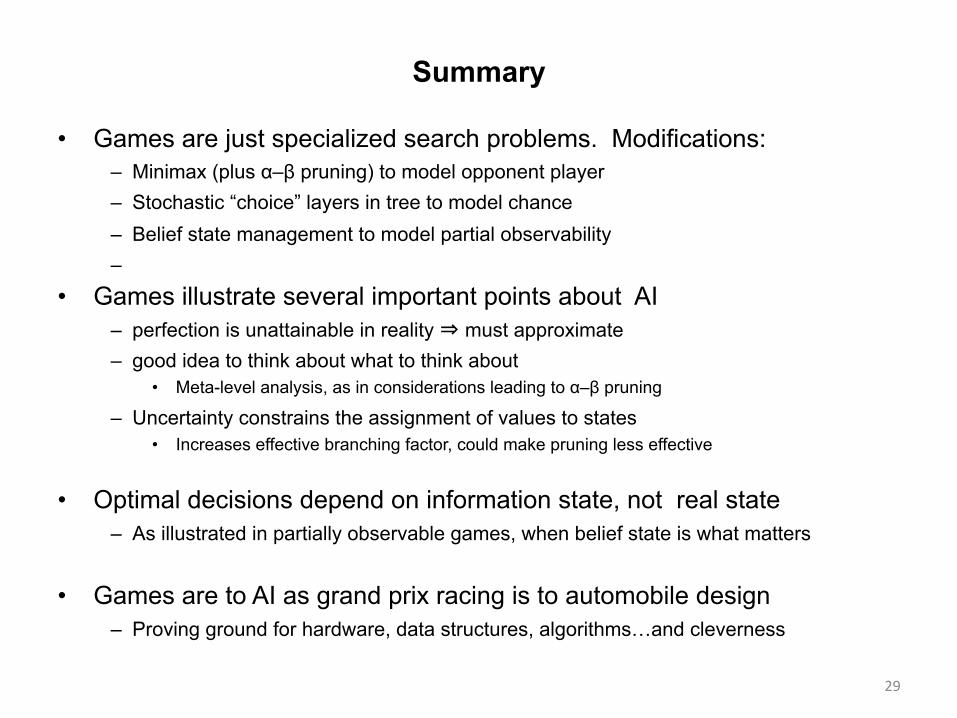
•  Games are just specialized search problems. Modifications: –  Minimax (plus α–β pruning) to model opponent player –  Stochastic “choice” layers in tree to model chance –  Belief state management to model partial observability – 

•  Games illustrate several important points about AI –  perfection is unattainable in reality ⇒ must approximate –  good idea to think about what to think about

•  Meta-level analysis, as in considerations leading to α–β pruning

–  Uncertainty constrains the assignment of values to states •  Increases effective branching factor, could make pruning less effective

•  Optimal decisions depend on information state, not real state –  As illustrated in partially observable games, when belief state is what matters

•  Games are to AI as grand prix racing is to automobile design –  Proving ground for hardware, data structures, algorithms…and cleverness

29

30