Advective balance in pipe-formed vortex rings∗

Karim Shariff†and Paul S. Krueger‡

December 19, 2017

Abstract

Vorticity distributions in axisymmetric vortex rings produced by a piston-pipe apparatus arenumerically studied over a range of Reynolds numbers, Re, and stroke-to-diameter ratios, L/D.It is found that a state of advective balance, such that ζ ≡ ωφ/r ≈ F (ψ, t), is achieved withinthe region (called the vortex ring bubble) enclosed by the dividing streamline. Here ζ ≡ ωφ/ris the ratio of azimuthal vorticity to cylindrical radius, and ψ is the Stokes streamfunction inthe frame of the ring. Some but not all of the Re dependence in the time evolution of F (ψ, t)can be captured by introducing a scaled time τ = νt, where ν is the kinematic viscosity. Whenνt/D2 & 0.02, the shape of F (ψ) is dominated by the linear-in-ψ component, the coefficient ofthe quadratic term being an order of magnitude smaller. An important feature is that as thedividing streamline (ψ = 0) is approached, F (ψ) tends to a non-zero intercept which exhibits anextra Re dependence. This and other features are explained by a simple toy model consisting ofthe one-dimensional cylindrical diffusion equation. The key ingredient in the model responsiblefor the extra Re dependence is a Robin-type boundary condition, similar to Newton’s law ofcooling, that accounts for the edge layer at the dividing streamline.

1 Introduction

1.1 Scope and Motivation

The present work numerically studies the vorticity distribution in laminar vortex rings producedby a piston-pipe apparatus at Reynolds numbers high enough that an edge layer, thinner than thesize of the ring, exists at the dividing streamline. The diagnostics to be presented focus on thevorticity distribution in the region interior to the dividing streamline, called the vortex ring bubble.A model shows that the boundary condition provided by the edge layer is needed to account foran extra Reynolds number dependence, in addition to that accounted for by introducing a scaledtime, τ = νt. However, the detailed structure of the edge layer and wake is not considered in thepresent work. We hope that it is elucidated in the future. For that effort, high Reynolds numberfalling drops (Harper & Moore, 1968) should provide a useful analogy: their structure also consistsof an advectively balanced state in the interior surrounded by an edge layer that sheds a wake.

One motivation for studying the laminar vorticity distribution is that azimuthal instabilitiesare sensitive to its precise form (Saffman, 1978). Another motivation is that the non-dimensional

∗J. Fluid Mech. (2018) 836, 773–796.†NASA Ames Research Center‡Southern Methodist University

1

arX

iv:1

712.

0590

3v1

[ph

ysic

s.fl

u-dy

n] 1

6 D

ec 2

017

energy, E ≡ E/(I1/2Γ3/2

), which determines the limiting stroke-to-diameter ratio according to

Gharib et al. (1998), depends on the peakiness of the vorticity profile. (Here E is the kineticenergy, I is the impulse, and Γ is the circulation; density is set to unity.) For example, Hill’s

spherical vortex which has uniform ζ ≡ ωφ/r gives E = 0.16 while the experimentally measured

value for the limiting ring is a much larger E ≈ 0.33. In addition, the dividing streamline of Hill’svortex has zero oblateness (a− b)/b while the thickest experimental ring has an oblateness of 0.21as inferred from photographs in Gharib et al. (1998), a and b being the semi-major and minor axes,respectively. The discrepancies in energy and oblateness are both consequences of the peakiness ofζ in actual rings.

The family of steady vortex rings (Norbury, 1973) with uniform ζ, in which Hill’s vortex isthe thickest member, has been used to model vortex ring formation (Mohseni & Gharib, 1998;

Shusser & Gharib, 2000; Linden & Turner, 2001). Since thinner rings have larger E, the result inthese studies is that the limiting ring corresponds to a thinner member of the family than Hill’svortex. If one were to use a family of rings having a more realistic peaked vorticity distribution,the result would presumably be that the limiting experimental ring corresponds better with thethickest member of that family.

The physics of vortex sheet roll-up at an edge implies a peaked distribution of ζ. Saffman (1978)and Pullin (1979) obtain the form of ζ for thin rings (and in the inner region of the core) by usingKirde’s (1962) theory for two-dimensional vortex sheet roll-up at an edge. This theory gives thevorticity in terms of the hypergeometric function. For thicker rings, there is a calculation of theirformation from axisymmetric vortex sheet roll-up (Nitsche & Krasny, 1994), but no correspondingprediction of the vorticity distribution. We hope that this lack is addressed soon.

1.2 Present work

The vorticity equation is Dζ/Dt = 0 for inviscid swirl-free axisymmetric flow. Hence if the flow issteady in some uniformly propagating frame, we have

ζ = F (ψ), (1)

where ψ is the Stokes streamfunction in the ring frame. It is natural to wonder if viscous vortexrings generated in the laboratory obey (1) and if so, what form F (ψ) takes. Knowing this, onecould solve for the main structure of the ring (i.e., apart from the wake and edge layer) by solvingan elliptic free boundary problem (Eydeland & Turkington, 1988). It was this possibility thatmotivated the present work.

The axisymmetric Navier-Stokes simulations performed here show that throughout the vortexring bubble (except very close to the dividing streamline), a state of ζ ≈ F (ψ, t) is reached after aperiod of relaxation. However, even after moderately large times, F (ψ, t) is not a universal functionand depends on Reynolds number, Re, and stroke-to-diameter ratio L/D. The best that can besaid is that F (ψ, t) tends to an approximately linear function with a non-zero intercept, whosedependencies will be studied in the sequel.

For interpreting results, it is helpful to keep in mind some consequences of the vorticity equation.We adopt a reference frame moving with the ring at speed U(t). Because the frame is decelerating, afictitious force term −ρU x, is present on the right-hand-side of the equation for momentum per unitvolume. However, for uniform density, ρ, this term can be absorbed into the pressure: p→ p+ρUx.

2

Thus, the vorticity equation remains unchanged in the moving frame:

∂ω

∂t+ u · ∇ω = ω · ∇u + ν∇2ω. (2)

For axisymmetric swirl-free flow in cylindrical coordinates (Batchelor 1967, pg. 602), equation (2)becomes

Dζ

Dt≡ ∂ζ

∂t+ ux

∂ζ

∂x+ ur

∂ζ

∂r= ν

(∂2ζ

∂x2+∂2ζ

∂r2+

3

r

∂ζ

∂r

), (3)

where

ux =1

r

∂ψ

∂r, ur = −1

r

∂ψ

∂x, (4)

defines the Stokes streamfunction ψ. Note that for inviscid flow ζ ≡ ωφ/r is conserved followingfluid elements; the r in the denominator accounts for vorticity stretching. Suppose that at a giveninstant we have ζ = F (ψ, t) in a certain region of the flow. The simulations will show that thisis approximately the case within the vortex ring bubble. Then by direct substitution into (3) onesees that the advection terms sum to zero, which is called advective balance. This does not implythat the subsequent evolution is viscous. The diffusion operator in (3) destroys advective balancewhen the ring is not thin; see §81. It is suggested that maintenance of the condition ζ ≈ F (ψ, t)requires that non-linear terms still be active. A solution for the time evolution of F (ψ, t) must takeadvective effects into account and §81 conjectures that this effect is shear dispersion which leads toaveraging of the vorticity field on a closed streamline. A similar suggestion was made by Rhines &Young (1983) for planar vortices.

1.3 Previous efforts

Berezovski & Kaplanski (1987) obtained a time-dependent Stokes-flow vortex ring solution witha peaked vorticity distribution. This solution has zero thickness at νt = 0 and tends to the self-similar solution obtained by Phillips (1956) as νt→∞. No advection effects are present aside froma spatially uniform drift, which was obtained by Kaplanski & Rudi (2001) using the proceduresof Kambe & Oshima (1975) and Rott & Cantwell (1993a,b). Kaplanski & Rudi (2005) obtain the

value of νt at which the non-dimensional energy E of the Stokes solution equals the value 0.33 ofthe experimental limiting ring. Interestingly, at this value of νt, the non-dimensional circulationand ring speed also roughly match experimental values. This suggests that the Stokes flow solutiondoes capture some of the overall properties of high Reynolds number rings.

A virtue of the Stokes solution is that it fully includes curvature effects for vorticity diffusion.However, some issues arise because vorticity advection is absent: (i) Since the vorticity field is notdeformed by the curvature-induced strain, vorticity contours are not axially elongated as in actualhigh Reynolds number rings. To overcome this difficulty, Kaplanski et al. (2012) introduce axialelongation and radial compression factors into the vorticity field of the Stokes solution. The valuesof the two factors are selected by matching the non-dimensional energy and circulation of the modelring against values obtained from Navier-Stokes simulations. (ii) An edge layer, where advectionand viscous terms nearly balance, is missing. (iii) Since viscosity enters the vorticity field of theStokes solution only via the product νt, the solution cannot exhibit the extra Reynolds numberdependence observed in the present results. (iv) Since the viscous term acts to destroy advectivebalance, the Stokes ring cannot in general satisfy advective balance except at early times when thering is thin.

3

pressure

outlet

wall (no slip)

axis

≥ 15D (Nx nodes)

3D

Up(t) D/2

3.5D

(Nr

no

de

s)

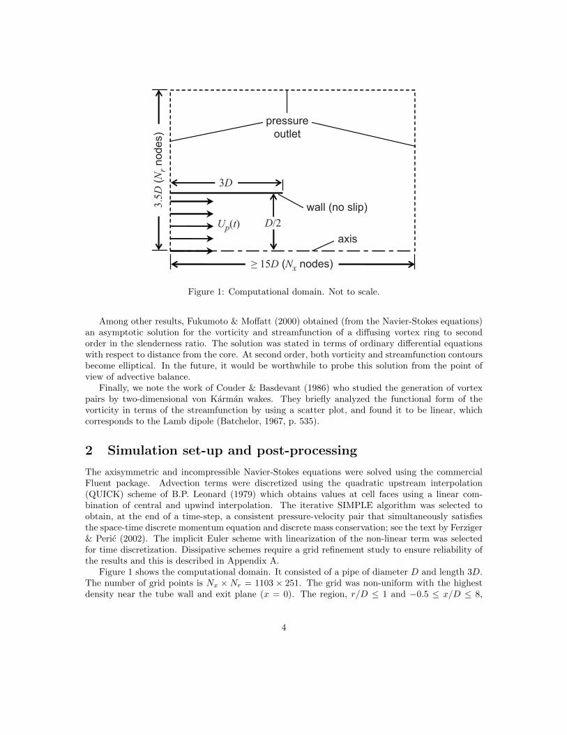
Figure 1: Computational domain. Not to scale.

Among other results, Fukumoto & Moffatt (2000) obtained (from the Navier-Stokes equations)an asymptotic solution for the vorticity and streamfunction of a diffusing vortex ring to secondorder in the slenderness ratio. The solution was stated in terms of ordinary differential equationswith respect to distance from the core. At second order, both vorticity and streamfunction contoursbecome elliptical. In the future, it would be worthwhile to probe this solution from the point ofview of advective balance.

Finally, we note the work of Couder & Basdevant (1986) who studied the generation of vortexpairs by two-dimensional von Karman wakes. They briefly analyzed the functional form of thevorticity in terms of the streamfunction by using a scatter plot, and found it to be linear, whichcorresponds to the Lamb dipole (Batchelor, 1967, p. 535).

2 Simulation set-up and post-processing

The axisymmetric and incompressible Navier-Stokes equations were solved using the commercialFluent package. Advection terms were discretized using the quadratic upstream interpolation(QUICK) scheme of B.P. Leonard (1979) which obtains values at cell faces using a linear com-bination of central and upwind interpolation. The iterative SIMPLE algorithm was selected toobtain, at the end of a time-step, a consistent pressure-velocity pair that simultaneously satisfiesthe space-time discrete momentum equation and discrete mass conservation; see the text by Ferziger& Peric (2002). The implicit Euler scheme with linearization of the non-linear term was selectedfor time discretization. Dissipative schemes require a grid refinement study to ensure reliability ofthe results and this is described in Appendix A.

Figure 1 shows the computational domain. It consisted of a pipe of diameter D and length 3D.The number of grid points is Nx × Nr = 1103 × 251. The grid was non-uniform with the highestdensity near the tube wall and exit plane (x = 0). The region, r/D ≤ 1 and −0.5 ≤ x/D ≤ 8,

4

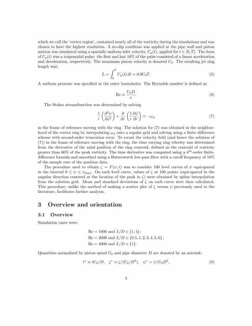
which we call the ‘vortex region’, contained nearly all of the vorticity during the simulations and waschosen to have the highest resolution. A no-slip condition was applied at the pipe wall and pistonmotion was simulated using a spatially uniform inlet velocity, Up(t), applied for t ∈ [0, T ]. The formof Up(t) was a trapezoidal pulse: the first and last 10% of the pulse consisted of a linear accelerationand deceleration, respectively. The maximum piston velocity is denoted U0. The resulting jet sluglength was:

L =

∫ T

0

Up(t) dt = 0.9U0T. (5)

A uniform pressure was specified at the outer boundaries. The Reynolds number is defined as

Re ≡ U0D

ν. (6)

The Stokes streamfunction was determined by solving

1

r

(∂2ψ

∂x2

)+

∂

∂r

(1

r

∂ψ

∂r

)= −ωφ (7)

in the frame of reference moving with the ring. The solution for (7) was obtained in the neighbor-hood of the vortex ring by interpolating ωφ onto a regular grid and solving using a finite differencescheme with second-order truncation error. To recast the velocity field (and hence the solution of(7)) in the frame of reference moving with the ring, the time varying ring velocity was determinedfrom the derivative of the axial position of the ring centroid, defined as the centroid of vorticitygreater than 60% of the peak vorticity. The time derivative was computed using a 4th-order finite-difference formula and smoothed using a Butterworth low-pass filter with a cutoff frequency of 10%of the sample rate of the position data.

The procedure used to obtain ζ = F (ψ, t) was to consider 100 level curves of ψ equi-spacedin the interval 0 ≤ ψ ≤ ψmax. On each level curve, values of ζ at 100 points (equi-spaced in theangular direction centered at the location of the peak in ζ) were obtained by spline interpolationfrom the solution grid. Mean and standard deviations of ζ on each curve were then calculated.This procedure, unlike the method of making a scatter plot of ζ versus ψ previously used in theliterature, facilitates further analysis.

3 Overview and orientation

3.1 Overview

Simulation cases were:

Re = 1000 and L/D ∈ {1, 4} ;

Re = 2000 and L/D ∈ {0.5, 1, 2, 3, 4, 5, 6} ;

Re = 4000 and L/D ∈ {1} .

Quantities normalized by piston speed U0 and pipe diameter D are denoted by an asterisk:

t∗ ≡ tU0/D, ζ∗ ≡ ζ/(U0/D2), ψ∗ = ψ/U0D

2, (8)

5

and a hat is used for ζ and ψ normalized by their peak values (which decay in time):

ζ ≡ ζ/ζmax(t), ψ ≡ 1− ψ/ψmax(t). (9)

To diagnose the shape of ζ(ψ) at different instants, coefficients of the least-squares cubic

ζfit(ψ, t) = 1− a1(t)ψ + a2(t)ψ2 + a3(t)ψ3, (10)

fit to the data are obtained. Only the mean value of ζ on each streamline was used for the fit.To avoid the edge layer, the last value included in the fit is ψ = 0.99. To ensure that ζ = F (ψ, t)to a good approximation, results of the fit and any quantity derived from it is plotted only if thestandard deviation of ζ on every sampled streamline is < 0.04 for 0 ≤ ψ ≤ 0.99, and the rms errorof the cubic fit is < 0.005. After a referee’s comment, a least squares fit was also performed to theform

ζfit2(ψ, t) = exp(−b1(t)ψ + b2(t)ψ2 + b3(t)ψ3

), (11)

In only a small fraction of the fields (0 to 16% for any given case) was it found to give a smallerrms error than the cubic.

A diagnostic of interest will be the value of ζ as the dividing streamline is approached from theinterior of the ring bubble: ζ(ψ → 1−). The use of a limit acknowledges the presence of an edgelayer governed by boundary layer type behaviour which should match the interior flow. The limitshould be thought of in the same way that one thinks of the limit of potential flow past a body asthe surface is approached, which should match the outer limit of the boundary layer. The limit isobtained from the computations as

ζ(ψ → 1−) = ζfit(ψ = 1), (12)

which represents a slight extrapolation since the last value included in the fit is ψ = 0.99.

3.2 Orientation

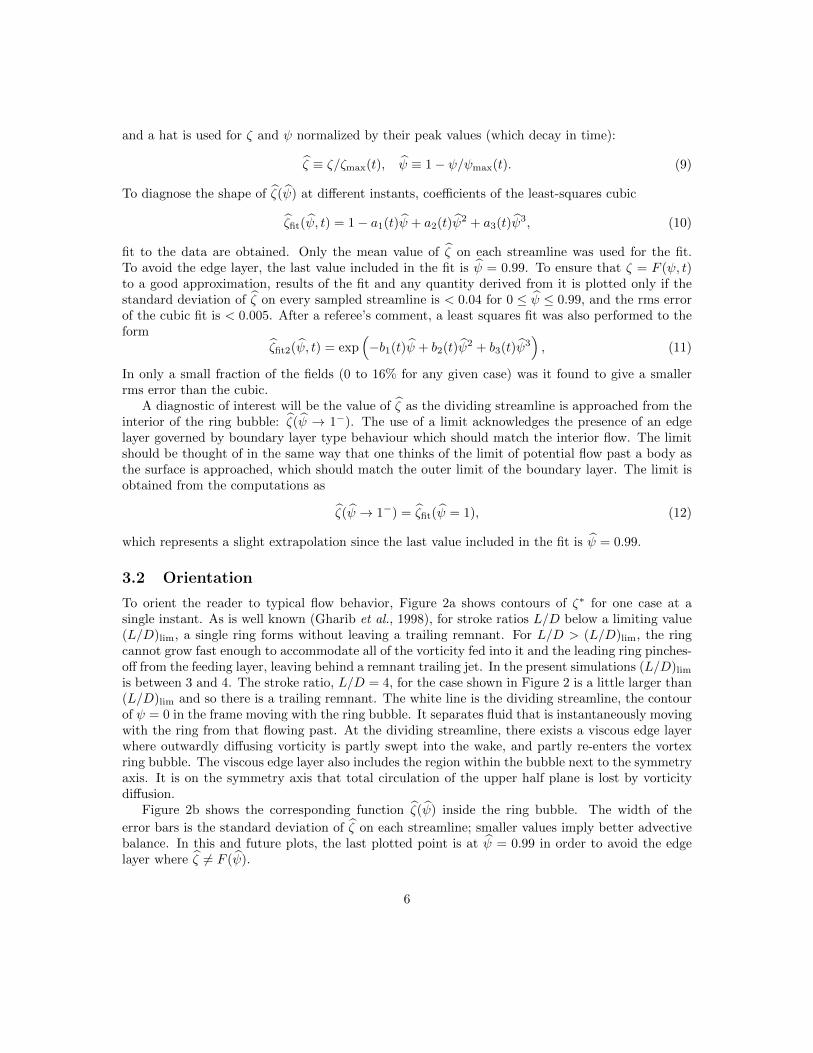
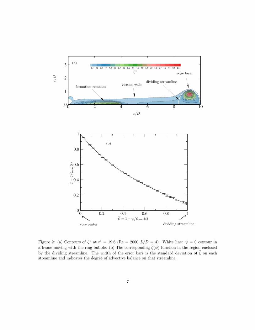
To orient the reader to typical flow behavior, Figure 2a shows contours of ζ∗ for one case at asingle instant. As is well known (Gharib et al., 1998), for stroke ratios L/D below a limiting value(L/D)lim, a single ring forms without leaving a trailing remnant. For L/D > (L/D)lim, the ringcannot grow fast enough to accommodate all of the vorticity fed into it and the leading ring pinches-off from the feeding layer, leaving behind a remnant trailing jet. In the present simulations (L/D)lim

is between 3 and 4. The stroke ratio, L/D = 4, for the case shown in Figure 2 is a little larger than(L/D)lim and so there is a trailing remnant. The white line is the dividing streamline, the contourof ψ = 0 in the frame moving with the ring bubble. It separates fluid that is instantaneously movingwith the ring from that flowing past. At the dividing streamline, there exists a viscous edge layerwhere outwardly diffusing vorticity is partly swept into the wake, and partly re-enters the vortexring bubble. The viscous edge layer also includes the region within the bubble next to the symmetryaxis. It is on the symmetry axis that total circulation of the upper half plane is lost by vorticitydiffusion.

Figure 2b shows the corresponding function ζ(ψ) inside the ring bubble. The width of the

error bars is the standard deviation of ζ on each streamline; smaller values imply better advectivebalance. In this and future plots, the last plotted point is at ψ = 0.99 in order to avoid the edgelayer where ζ 6= F (ψ).

6

0 2 4 6 8 100

1

2

30.1 0.5 0.9 1.4 1.8 2.3 2.7 3.2 3.6 4.1 4.5 4.9 5.4 5.8 6.3 6.7 7.2 7.6 8.1 8.5

x/D

r/D

ζ∗

formation remnantviscous wake

edge layer

dividing streamline

(a)

0 0.2 0.4 0.6 0.8 10

0.2

0.4

0.6

0.8

1

dividing streamlinecore center

(b)

ψ = 1− ψ/ψmax(t)

ζ=ζ/ζ m

ax(t)

Figure 2: (a) Contours of ζ∗ at t∗ = 19.6 (Re = 2000, L/D = 4). White line: ψ = 0 contour in

a frame moving with the ring bubble. (b) The corresponding ζ(ψ) function in the region enclosed

by the dividing streamline. The width of the error bars is the standard deviation of ζ on eachstreamline and indicates the degree of advective balance on that streamline.

7

4 Model: One-dimensional radial diffusion with an edge layer

A one-dimensional toy model based on vorticity diffusion in a cylindrical (and non-curved) vortextube is presented here. It was developed to explain the extra Reynolds number dependence observedfor the vorticity on the dividing streamsurface, specifically, for the ratio ζ(ψ → 0)/ζmax(t). Thekey ingredient in the model is a condition at the boundary of the vortex tube which accounts forthe viscous layer at the dividing streamsurface of actual vortex rings. The model assumes that theedge layer is circular which is not true even for thin rings. Hence the model is not a mathematicalsolution in any asymptotic limit and should be viewed as being merely illustrative.

For a thin vortex ring, i.e., one whose core radius δcore � R (the toroidal radius), variations inr across the cross-section of the tube can be neglected, i.e., r = R(1 +O (δcore/R)). The vorticitydynamics is then locally (i.e., within the tube and in the co-moving frame) the same as for planarflow. Therefore, if the vortex initially has concentric circular streamlines and vorticity contours,they will continue to remain so. Therefore, it is reiterated that the model does not account forthe effect of curvature-induced strain on the diffusion of vorticity in the interior of the vortex ringbubble.

A feature of circular streamline flow is that the advective terms are trivially zero and theazimuthal vorticity ωφ obeys the planar diffusion equation

∂ωφ∂t

= ν1

s

∂

∂s

(s∂ωφ∂s

), 0 ≤ s ≤ sDS(t), (13)

where s is radial distance measured from the center of the core in a meridional plane, and sDS(t) isthe distance to the boundary of the vortex tube; it is allowed to grow in time as the ring expands.Equation (13) is solved numerically.

Next comes an assumption that makes the treatment an illustrative model (even for a thin ring)rather than a rigorous analysis: (13) will be applied all the way out to the dividing streamline(denoted using subscript DS) at which location, neither local two-dimensionality holds nor arestreamlines circular. The distance from the core center to the notional dividing streamline isdenoted as sDS(t) which represents roughly the average distance from the center of the ring to theactual dividing streamline.

At the dividing streamline of an actual ring there is an edge layer whose thickness δlayer (averagedalong the length of the streamline, say) is

δlayer ∝ (ν/ε)1/2

, (14)

where

ε ∝ ring speed

R(t)∝ Γ(t)/4πR(t)2, (15)

is the characteristic strain-rate to which the layer is subject. The boundary condition applied tothe diffusion equation (13) to model the edge layer is

∂ωφ∂s

∣∣∣∣s=sDS

= −Cmodelωφ(s = sDS)

δlayer, (16)

where Cmodel is a modeling constant which allows one to change all ∝ into = signs. Combining(14) and (15) one sees that

δlayer = 2√π(Γ(t)/ν)−1/2R(t) (17)

8

involves the instantaneous ring Reynolds number Γ(t)/ν, a fact that will be important in the sequel.The asymptotic analysis of Fukumoto & Moffatt (2000) revealed that to third order in core

thickness, the radius of a diffusing ring grows linearly in time:

R(t) = R0 + CFMν(t− T )/R0. (18)

The rate of growth is different for the radius corresponding to the peak vorticity and the radiuscorresponding to the peak value of the co-moving streamfunction, the respective values of CFM

being 4.59 and 2.59. (Note that this difference implies loss of advective balance.) Tests with themodel revealed that the value of CFM influenced the decay rate of ψ∗max(t) plotted in Figure 4e.We chose CFM = 2.9 to obtain the best agreement between the model and simulation for ψ∗max(t).Ring expansion is not critical to the model and was included only to improve the postdiction ofψ∗max(t).

We set Cmodel = 2.2 and sDS(t)/R(t) = 0.50 based on a visual matching of model and simulationresults for the L/D = 1,Re = 1000 case. The boundary condition (16) is of Robin-type becauseit involves a linear combination of value and derivative; it is analogous to Newton’s law of coolingwhich is used to represent a layer of advective cooling at the surface of a heat conducting solid.Ring vorticity is undergoing a similar advective-diffusive process in the edge layer. Note thatthe boundary condition (16) is non-linear in the vorticity due to the presence of Γ(t), which is afunctional of the vorticity.

The initial vorticity profile for the diffusion equation in terms of piston parameters is prescribedin Appendix B. This initial profile, which also depends on ν, uses the theory of self-similar vortexsheet roll-up and is valid for thin cores.

To obtain the streamfunction as a diagnostic and to plot profiles of ζ(ψ), we first calculateζ ≡ ωφ/r, which ≈ ωφ/R to consistent order. The circumferential velocity, uθ(s), is then obtainedfrom

uθ(s) =1

s

∫ s

0

ωφs′ ds′. (19)

The co-moving two-dimensional streamfunction, ψ2D, is obtained by integrating

uθ = −∂ψ2D

∂s, (20)

from which, finally, the Stokes streamfunction is ψ = Rψ2D+C1 to consistent order. The integrationconstant C1 is chosen to make ψ = 0 at the notional dividing streamline s = sDS.

5 ζ(ψ, t) for a thin Gaussian ring

A referee requested comparison of vorticity profiles from the simulation against those for a thinGaussian ring (Saffman, 1970). This solution has circular vorticity contours which is true in thesimulations only for small L/D at early times. Nevertheless, because it is a simple analytical modelfor a diffusing ring, its ζ(ψ) profile provides a useful reference even outside its range of validity. Itshould be noted that while the experiments of Cater et al. (2004) obtained Gaussian-like vorticityprofiles, they were thinner in the radial direction than the axial direction due to the effect of strain.

The relations necessary for plotting ζ(ψ, t) for the Gaussian ring are presented below. Note thatin making a comparison with simulations, the relations will be evaluated all the way to the dividingstreamline which is outside their range of validity, s � R, even for thin rings (as before, s is the

9

distance from the center of the core in a meridional plane). The ring radius (R) and circulation (Γ)needed to evaluate the relations are, as for the model described in the previous section, obtainedfrom the expressions in Appendix B.

When σ(t) (the core radius) � R, the dynamics are locally two-dimensional and the two-dimensional Oseen (Gaussian) vortex is a valid local solution for ωφ, and therefore

ζ(s, t) ≡ ωφr

=Γ

πσ2rexp(−s2/σ2) [1 +O (s/R)] , σ = σ(t). (21)

The speed of such a ring, needed later, was calculated by Saffman (1970) as

U(t) =Γ

4πR

[log

(8R

σ

)− 0.558 +O

(σ2

R2log

σ

R

)]. (22)

Integrating the circumferential velocity of Oseen’s vortex gives its streamfunction:

ψ2D(s, t) = − Γ

2π

[log

s

σ+

1

2E1(s2/σ2)

], (23)

where E1 is the exponential integral and the integration constant was chosen to non-dimensionalizethe argument of the logarithm. The local Stokes streamfunction for the vortex ring is

ψ(s, t) = Rψ2D [1 +O(s/R)] + C2, s� R. (24)

The constant C2 is not disposable and is obtained by using the asymptotic matching rule describedby Moore (1980) in his calculation of the speed of an elliptical core ring. The rule is that in theregion σ � s� R, equation (24) should match the streamfunction for a zero thickness ring in theregion s� R, which is given by Moore’s equation (2.27):

ψ0 =ΓR

2π

[log

(8R

s

)− 2 +O

( sR

)]− 1

2U(t)R2. (25)

Matching gives

C2 =ΓR

2π

[log

8R

σ− 2

]− 1

2U(t)R2. (26)

Equations (21) and (24) implicitly give ζ(ψ) for the Gaussian ring. The slope of this function canbe obtained explicitly at the core center:

dζ

dψ=

1

R2

dωφds

(dψ2D

ds

)−1

= − 1

R2

1

uθ(s)

dωφds

=4

R2σ2(t)(27)

at s = 0.The behaviour of the core size is specified as

σ(t)2 = σ20 + 4ν(t− T ), (28)

where σ0 is the core size at the end of the piston stroke. To obtain σ0, we note that for thehypergeometric profile (eq. 39 in Appendix B) the radius of peak velocity is (Saffman, 1978)

s1 = 1.45 (4νT )1/2

(29)

10

at the end of the piston stroke. On the other hand, the radius of peak velocity for the Gaussianvortex is

s1 = 1.121σ0. (30)

Equating (29) and (30) givesσ0 = 1.29(4νT )1/2. (31)

Since the circulation of the Gaussian ring is assumed to be constant, growth of radius would implyincreasing impulse ∝ ΓR2. Hence its radius is kept fixed at its initial value.

6 Results

6.1 Re dependence at L/D = 1

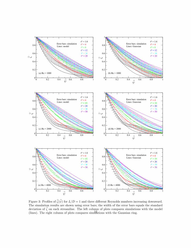
Figure 3 shows profiles of ζ(ψ, t) for L/D = 1 and three Reynolds numbers. The left column of plotscompares simulation results (error bars) with the model (lines); the width of the error bars equals

the standard deviation of ζ on each streamline. The right column of plots compares simulationswith the Gaussian ring. A small value for the standard deviation means that the vorticity is inapproximate advective balance; this is achieved earlier and better for higher Re. Vorticity diffusioncauses the profiles to become less curved with time, which happens slower with increasing Re asexpected. It is noteworthy that the value of ζ(ψ → 1−), i.e., as the dividing streamline is approached

and ignoring the edge layer, is non-zero. The value of ζ(ψ → 1−) increases with time and decreaseswith Reynolds number. At early times, the profiles for the model and Gaussian ring do not haveas much vorticity in the middle region of the bubble (ψ ≈ 0.5) as the simulation does; this reflectsinaccuracy in the initial condition provided by the vortex sheet roll-up theory (Appendix B). Forthe highest Re case, a small secondary vorticity peak, which represents an outer spiral turn, isobserved in this region. The distance between adjacent spiral turns is larger than the diffusionlength in this region (Pullin, 1979).

The model initially lags the simulation in its development towards an approximately linearprofile and then leads at later times. Overall, the Gaussian ring gives a similar degree of agreementwith the simulation as the model does, its most obvious error being a significant overshoot in thevalue of ζ(ψ → 1−) at late times. This occurs because there is no edge layer to sweep away diffusedvorticity.

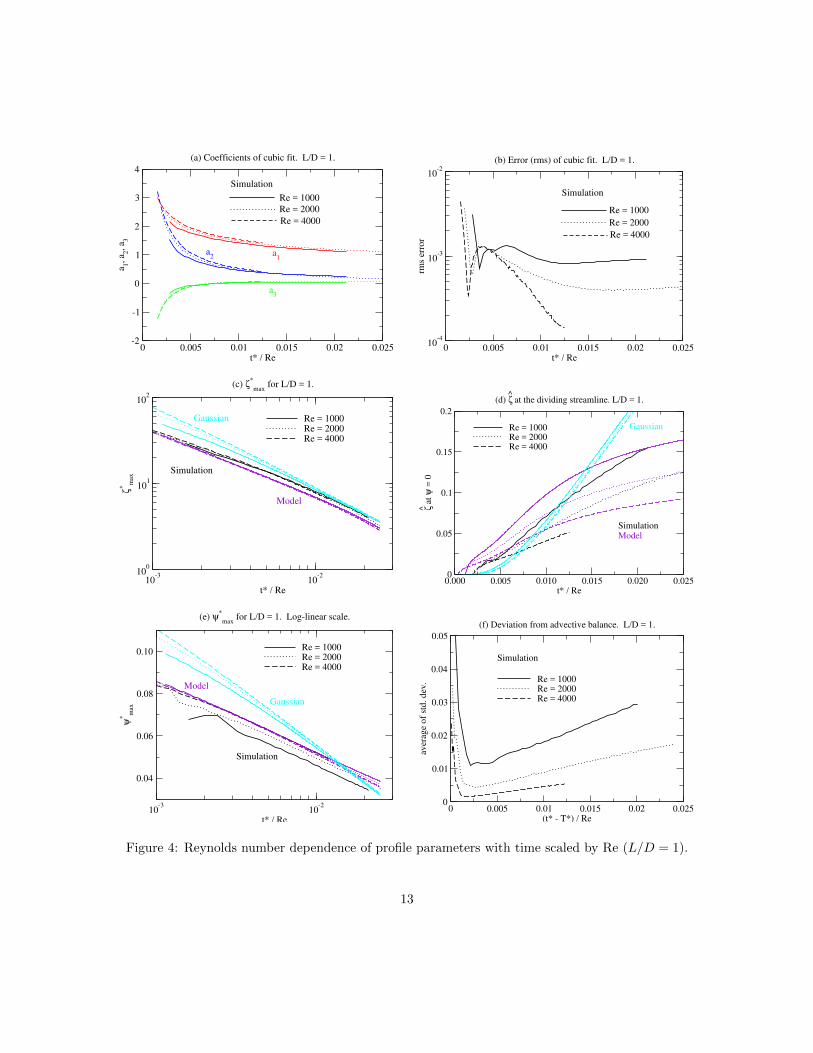
Figure 4 shows the evolution of various parameters of the vorticity profile with respect tot∗/Re = νt/D2. Figure 4a displays the evolution of the cubic coefficients which are plotted onlyafter the rms error (Figure 4b) of the cubic fit becomes < 0.005. With time left unscaled, therewas considerable difference in the curves (not shown) for the three Re cases. Scaling time by Rereduces this difference due to the important role of viscosity in the overall evolution of ζ(ψ, t).Some extra Re dependence of the coefficients remains and this must ultimately be accounted for byReynolds number effects in (i) the ring formation process, (ii) the boundary condition at the edgelayer, and (iii) the competition between viscous destruction of advective balance and its restorationby non-linear terms.

As t∗/Re increases, the linear coefficient a1 tends to approximately unity, while a2 and a3 tendto approximately zero. This means that the profile becomes approximately linear with a smallintercept equal to (1− a1) + a2 + a3 at the dividing streamsurface, ψ → 1−.

Figure 4c shows that the decay of the peak vorticity (ζ∗max) for the three Re cases curves collapsesquite well (but not perfectly) when time is scaled using Re. The three violet colored curves (which

11

0 0.2 0.4 0.6 0.8 10

0.2

0.4

0.6

0.8

1

(a) Re = 1000

t* = 1.6

t* = 4

t* = 8

t* = 12

t* = 16

t* = 20

Error bars: simulation

Lines: model

ψ

ζ

0 0.2 0.4 0.6 0.8 10

0.2

0.4

0.6

0.8

1

(b) Re = 1000

t* = 1.6

t* = 4

t* = 8

t* = 12

t* = 16

t* = 20

Error bars: simulation

Lines: Gaussian

ψ

ζ

0 0.2 0.4 0.6 0.8 10

0.2

0.4

0.6

0.8

1

(c) Re = 2000

t* = 1.6

t* = 4

t* = 10

t* = 20

t* = 30

t* = 50

Error bars: simulation

Lines: model

ψ

ζ

0 0.2 0.4 0.6 0.8 10

0.2

0.4

0.6

0.8

1

(d) Re = 2000

t* = 1.6

t* = 4

t* = 10

t* = 20

t* = 30

t* = 50

Error bars: simulation

Lines: Gaussian

ψ

ζ

0 0.2 0.4 0.6 0.8 10

0.2

0.4

0.6

0.8

1

(e) Re = 4000

t* = 1.6

t* = 4

t* = 10

t* = 20

t* = 30

t* = 50

Error bars: simulation

Lines: model

ψ

ζ

0 0.2 0.4 0.6 0.8 10

0.2

0.4

0.6

0.8

1

(f) Re = 4000

t* = 1.6

t* = 4

t* = 10

t* = 20

t* = 30

t* = 50

Error bars: simulation

Lines: Gaussian

ψ

ζ

Figure 3: Profiles of ζ(ψ) for L/D = 1 and three different Reynolds numbers increasing downward.The simulation results are shown using error bars; the width of the error bars equals the standarddeviation of ζ on each streamline. The left column of plots compares simulations with the model(lines). The right column of plots compares simulations with the Gaussian ring.12

0 0.005 0.01 0.015 0.02 0.025t* / Re

-2

-1

0

1

2

3

4

a 1, a 2

, a 3

(a) Coefficients of cubic fit. L/D = 1.

Re = 1000

Re = 2000

Re = 4000

a1

a2

a3

Simulation

0 0.005 0.01 0.015 0.02 0.025t* / Re

10-4

10-3

10-2

rms

erro

r

(b) Error (rms) of cubic fit. L/D = 1.

Re = 1000

Re = 2000

Re = 4000

Simulation

10-3

10-2

t* / Re

100

101

102

ζ∗

max

Re = 1000Re = 2000Re = 4000

(c) ζ∗

max for L/D = 1.

Model

Gaussian

Simulation

0.000 0.005 0.010 0.015 0.020 0.025t* / Re

0

0.05

0.1

0.15

0.2

ζ^ a

t ψ

= 0

Re = 1000Re = 2000Re = 4000

(d) ζ^ at the dividing streamline. L/D = 1.

Model

Gaussian

Simulation

10-3

10-2

t* / Re

0.04

0.06

0.08

0.10

ψ∗

max

Re = 1000Re = 2000Re = 4000

(e) ψ∗

max for L/D = 1. Log-linear scale.

Model

Gaussian

Simulation

0 0.005 0.01 0.015 0.02 0.025(t* - T*) / Re

0

0.01

0.02

0.03

0.04

0.05

aver

age

of

std. dev

. Re = 1000Re = 2000Re = 4000

(f) Deviation from advective balance. L/D = 1.

Simulation

Figure 4: Reynolds number dependence of profile parameters with time scaled by Re (L/D = 1).

13

are nearly coincident) show that the one-dimensional model tracks the simulation results quite well;the maximum error is about 10%.

Figure 4d shows that the value of ζ as the dividing streamline is approached has a significantextra Reynolds number dependence. It was the need to explain this that prompted development ofthe model with an edge-layer, whose results (violet lines) give the correct qualitative behaviour.

In the context of the model, the extra Re dependence could arise from the presence of ν in boththe initial condition (Appendix B) and boundary condition (16). To ascertain which of the twowas more important, control runs with the model were performed for the three Reynolds numbersin which the initial profile was fixed at the form given by the model for Re = 2000. This resultedin only a very slight change compared to the model results in Figure 4d, indicating that most ofthe extra Re dependence comes from the edge-layer boundary condition rather than changes inthe initial profile. The Gaussian ring (cyan lines) exhibits an insignificant amount of extra Redependence that is very different than observed in the simulations and the model. This is becausethe Gaussian ring lacks an advective-diffusive edge layer and because ν enters the solution (mostly)via the product νt; the small extra Re dependence is due to the presence of 4νT in the initial coresize (31). The behaviour of ζ(t) for the Gaussian ring at the dividing streamline never goes throughan inflection point and therefore has the opposite sign for the curvature at large times.

Figure 4e shows the decay of the peak value, ψ∗max, of the streamfunction. The best straightlines were obtained with a logarithmic abscissa. The model agrees very well with the simulationsfor Re = 4000 while having a small constant error for the other two Reynolds numbers. The smallextra Reynolds dependence in ψ∗max is not predicted by the model.

Figure 4f assesses the deviation from advective balance in the simulations using the standarddeviation of ζ on each streamline averaged for 0 ≤ ψ ≤ 0.99. Note that the abscissa is measuredfrom the end of the piston stroke at t = T . At higher Re, advective balance is achieved to a greaterdegree and is destroyed more slowly with respect to t∗/Re. In Figure 4f the rate of destructionof advective balance with respect to t∗/Re is roughly proportional to Re−1, hence the rate withrespect to t∗ is roughly proportional to Re−2. The quadratic-in-ν rate of destruction suggests thatthe advective term plays a role in restoring advective balance. One also observes that advectivebalance reaches the 0.02 threshold earlier (with respect to t∗/Re) with increasing Re. The increasinglevel of advective imbalance is likely a result of decreasing Γ(t)/ν with time.

6.2 L/D dependence at Re = 2000

Recall that the limiting value of L/D beyond which the ring trails a jet or sheds some vorticityduring the formation process is 3 < (L/D)lim < 4 in the simulations. Model results are presentedfor only L/D ≤ 3: according to current understanding, there should be no L/D dependence forL/D ≥ (L/D)lim. The simulations will indicate that this is not the case for ψ∗max.

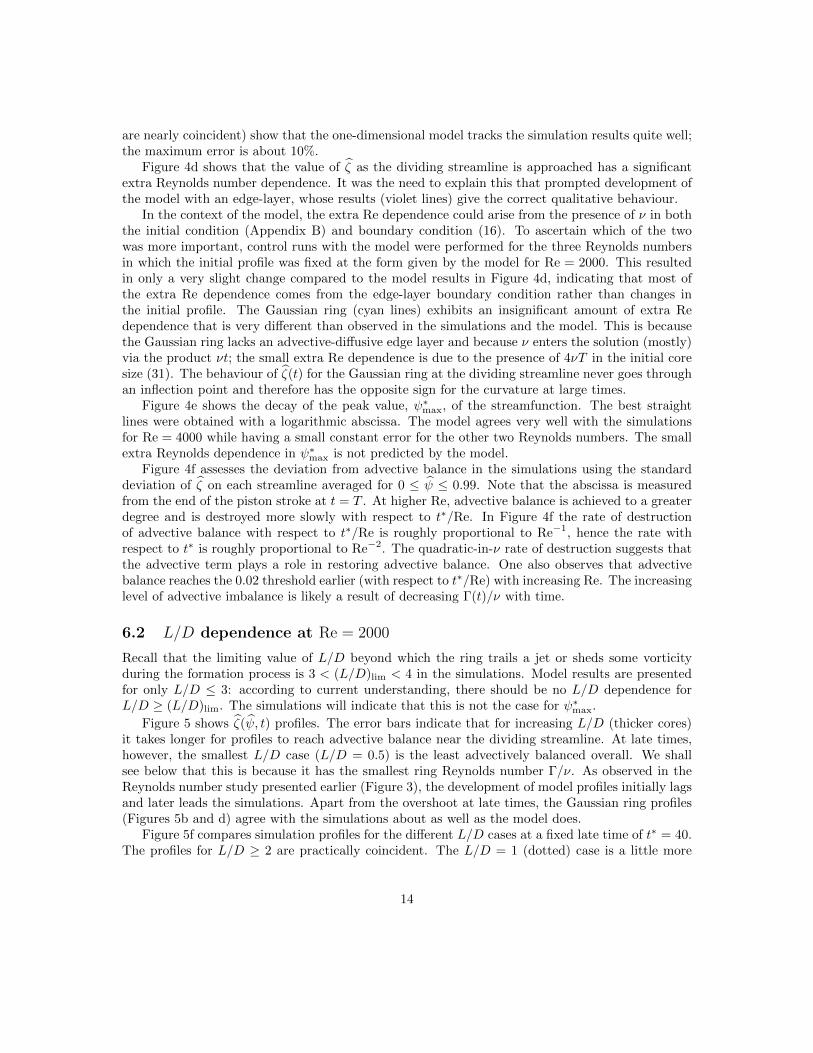
Figure 5 shows ζ(ψ, t) profiles. The error bars indicate that for increasing L/D (thicker cores)it takes longer for profiles to reach advective balance near the dividing streamline. At late times,however, the smallest L/D case (L/D = 0.5) is the least advectively balanced overall. We shallsee below that this is because it has the smallest ring Reynolds number Γ/ν. As observed in theReynolds number study presented earlier (Figure 3), the development of model profiles initially lagsand later leads the simulations. Apart from the overshoot at late times, the Gaussian ring profiles(Figures 5b and d) agree with the simulations about as well as the model does.

Figure 5f compares simulation profiles for the different L/D cases at a fixed late time of t∗ = 40.The profiles for L/D ≥ 2 are practically coincident. The L/D = 1 (dotted) case is a little more

14

0 0.2 0.4 0.6 0.8 10

0.2

0.4

0.6

0.8

1

(a) L/D = 0.5

t* = 1.6

t* = 4

t* = 10

t* = 20

t* = 30

t* = 50

Error bars: simulation

Lines: model

ψ

ζ

0 0.2 0.4 0.6 0.8 10

0.2

0.4

0.6

0.8

1

(b) L/D = 0.5

t* = 1.6

t* = 4

t* = 10

t* = 20

t* = 30

t* = 50

Error bars: simulation

Lines: Gaussian

ψ

ζ

0 0.2 0.4 0.6 0.8 10

0.2

0.4

0.6

0.8

1

(c) L/D = 2

t* = 4

t* = 10

t* = 20

t* = 30

t* = 40

t* = 50

Error bars: simulation

Lines: model

ψ

ζ

0 0.2 0.4 0.6 0.8 10

0.2

0.4

0.6

0.8

1

(d) L/D = 2

t* = 4

t* = 10

t* = 20

t* = 30

t* = 40

t* = 50

Error bars: simulation

Lines: Gaussian

ψ

ζ

0 0.2 0.4 0.6 0.8 10

0.2

0.4

0.6

0.8

1

(e) L/D = 4

t* = 8

t* = 20

t* = 30

t* = 40

t* = 50

Error bars: simulation

Lines: model

ψ

ζ

0 0.2 0.4 0.6 0.8 10

0.2

0.4

0.6

0.8

1

L/D = 0.5L/D = 1L/D = 2L/D = 3L/D = 4L/D = 5L/D = 6

(f) Simulaton profiles at t* = 40

ψ

ζ

Figure 5: Profiles of ζ(ψ) showing the dependence on L/D (Re = 2000).

15

diffuse, and the L/D = 0.5 (solid) case somewhat more diffuse than the rest. This is becausesmaller L/D rings have a smaller Γ0/ν and are therefore more diffusive.

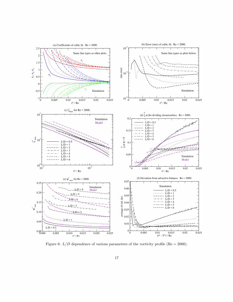
The cubic coefficients in Figure 6a show that differences in the shape of ζ(ψ) at early t∗/Rediminish later and the shape converges to a form that is weakly dependent on L/D; some variationand crossing of the curves at large times should be noted. The curve for a1 and L/D = 0.5 (solidred line) has a noticeable shift relative to the other curves perhaps due to its low ring Reynoldsnumber Γ(t)/ν.

The convergence noted in the previous paragraph is reminiscent of the study by Stanaway et al.(1988) of viscous vortex rings which found (pp. 74–76 in their work) that, for different initial corethicknesses (but same Γ0, ν, and R0), plots of normalized ring speed versus νt/R2

0 all converged toapproximately the same curve. In their plots, t is measured from a virtual origin when the ring hadzero core thickness.

Figure 6c displays the decay in peak vorticity, ζ∗max(t). The model works best for L/D = 1and has moderately large errors for the other L/D cases. These errors are present in the initialcondition and this suggests improvement of the relations in Appendix B.

Figure 6d shows ζ at the dividing streamline. At early times, a lower L/D produces a smallervalue of this quantity. This is expected since smaller L/D leads to a thinner core. However, a cross-

over occurs and eventually smaller L/D produces larger values of ζ(ψ → 1−) with unabated growthat the final instant of the simulation. This is non-intuitive at first sight, and it is hypothesized thatit is mainly due to smaller L/D rings having a smaller initial ring Reynolds number Γ0/ν. Sincethe trend of the dependence on L/D at large times is reproduced by the model, we can use it totest the hypothesis. We re-ran three L/D cases (L/D = 0.5, 1, and 2) using the model, but set theinitial circulation for all cases to the value for L/D = 2. Doing so reduced the range of variation

in ζmodel(ψ = 1, t∗/Re = 0.025) from [0.091, 0.152] to [0.091, 0.097]. Hence a substantial portion ofthe variation with respect to L/D is due to changing Γ0/ν.

Next we hypothesize that this effect of Γ0/ν (in the context of the model) enters mainly throughthe presence of Γ(t)/ν in the edge-layer boundary condition (17). To verify this, a test was performedin which Γ(t) in the model boundary condition was kept fixed in time at the Γ0 value for L/D = 2.

In this case the range of variation of ζmodel(ψ = 1, t∗/Re = 0.025) for the three L/D cases wasvery small, namely, [0.076, 0.078]. We conclude from this that a substantial portion of the L/D

dependence of ζ(ψ → 1−) is due to the dependence of edge layer physics on Γ(t)/ν, where Γ0

depends on L/D.To avoid clutter, results for the Gaussian ring have not been included in Figure 6. Suffice it to

say, it does not provide better predictions than the model.An important feature of the simulations which the model is unable to reproduce is that for

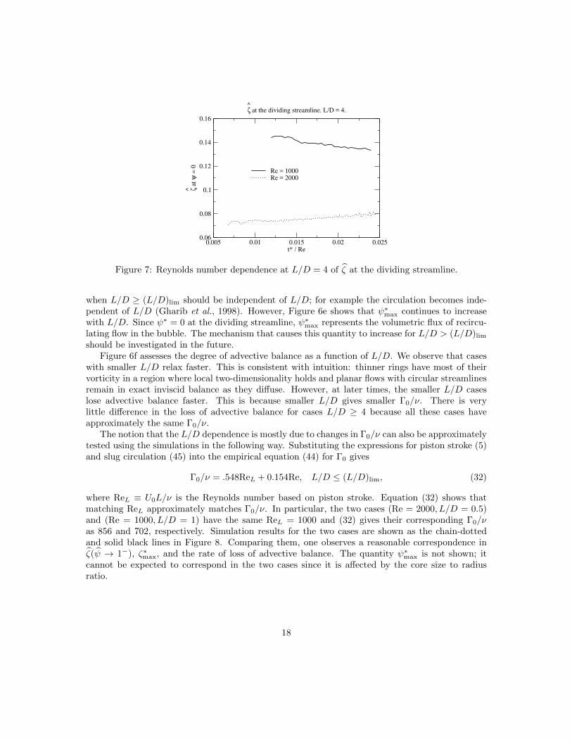
L/D ≥ 3, the temporal growth of ζ(ψ → 1−) saturates to a constant value. This constant valuehas a weak dependence on L/D for L/D ≥ 3. This is because Γ0/ν loses its dependence on L/Dfor L/D > (L/D)lim. The flat value for L/D = 4 decreases with Reynolds number as shown inFigure 7. Although the model is inaccurate at this value of L/D, we hypothesize on the basis ofprevious model results that this dependence mainly reflects the change in Γ0/ν which affects theedge layer.

Figure 6e shows that the peak value of the streamfunction increases with L/D, a trend that isalso captured by the model. However, the value of ψ∗max for L/D = 3 is over-predicted by a fairamount.

According to current thinking, the characteristics of the leading ring experimentally produced

16

0 0.005 0.01 0.015 0.02 0.025t* / Re

-1

-0.5

0

0.5

1

1.5

2

2.5

a 1,

a 2,

a 3

(a) Coefficients of cubic fit. Re = 2000.

a1

a2

a3

Same line types as other plots.

Simulation

0 0.005 0.01 0.015 0.02 0.025t* / Re

10-4

10-3

10-2

rms

erro

r

(b) Error (rms) of cubic fit. Re = 2000.

Simulation

Same line types as plots below.

10-3

10-2

t* / Re

100

101

102

ζ∗

max

L/D = 0.5L/D = 1L/D = 2L/D = 3L/D = 4L/D = 5L/D = 6

(c) ζmax

for Re = 2000.

Model

Simulation

0 0.005 0.01 0.015 0.02 0.025t* / Re

0

0.05

0.1

0.15

0.2

ζ^ a

t ψ

= 0

L/D = 0.5L/D = 1L/D = 2L/D = 3L/D = 4L/D = 5L/D = 6

(d) ζ^ at the dividing streamsurface. Re = 2000.

Model

Simulation

0.000 0.005 0.010 0.015 0.020 0.025t* / Re

0.00

0.05

0.10

0.15

0.20

0.25

ψ∗

max

(e) ψ∗

max for Re = 2000.

L/D = 6

L/D = 5

L/D = 4

L/D = 3

L/D = 2

L/D = 1

L/D = 0.5

ModelSimulation

0 0.005 0.01 0.015 0.02 0.025(t* - T*) / Re

0

0.01

0.02

0.03

0.04

0.05

0.06

0.07

aver

age

of

std

. d

ev.

L/D = 0.5L/D = 1L/D = 2L/D = 3L/D = 4L/D = 5L/D = 6

(f) Deviation from advective balance. Re = 2000.

Simulation

Figure 6: L/D dependence of various parameters of the vorticity profile (Re = 2000).

17

0.005 0.01 0.015 0.02 0.025t* / Re

0.06

0.08

0.1

0.12

0.14

0.16

ζ^ a

t ψ

= 0

Re = 1000Re = 2000

ζ^ at the dividing streamline. L/D = 4.

Figure 7: Reynolds number dependence at L/D = 4 of ζ at the dividing streamline.

when L/D ≥ (L/D)lim should be independent of L/D; for example the circulation becomes inde-pendent of L/D (Gharib et al., 1998). However, Figure 6e shows that ψ∗max continues to increasewith L/D. Since ψ∗ = 0 at the dividing streamline, ψ∗max represents the volumetric flux of recircu-lating flow in the bubble. The mechanism that causes this quantity to increase for L/D > (L/D)lim

should be investigated in the future.Figure 6f assesses the degree of advective balance as a function of L/D. We observe that cases

with smaller L/D relax faster. This is consistent with intuition: thinner rings have most of theirvorticity in a region where local two-dimensionality holds and planar flows with circular streamlinesremain in exact inviscid balance as they diffuse. However, at later times, the smaller L/D caseslose advective balance faster. This is because smaller L/D gives smaller Γ0/ν. There is verylittle difference in the loss of advective balance for cases L/D ≥ 4 because all these cases haveapproximately the same Γ0/ν.

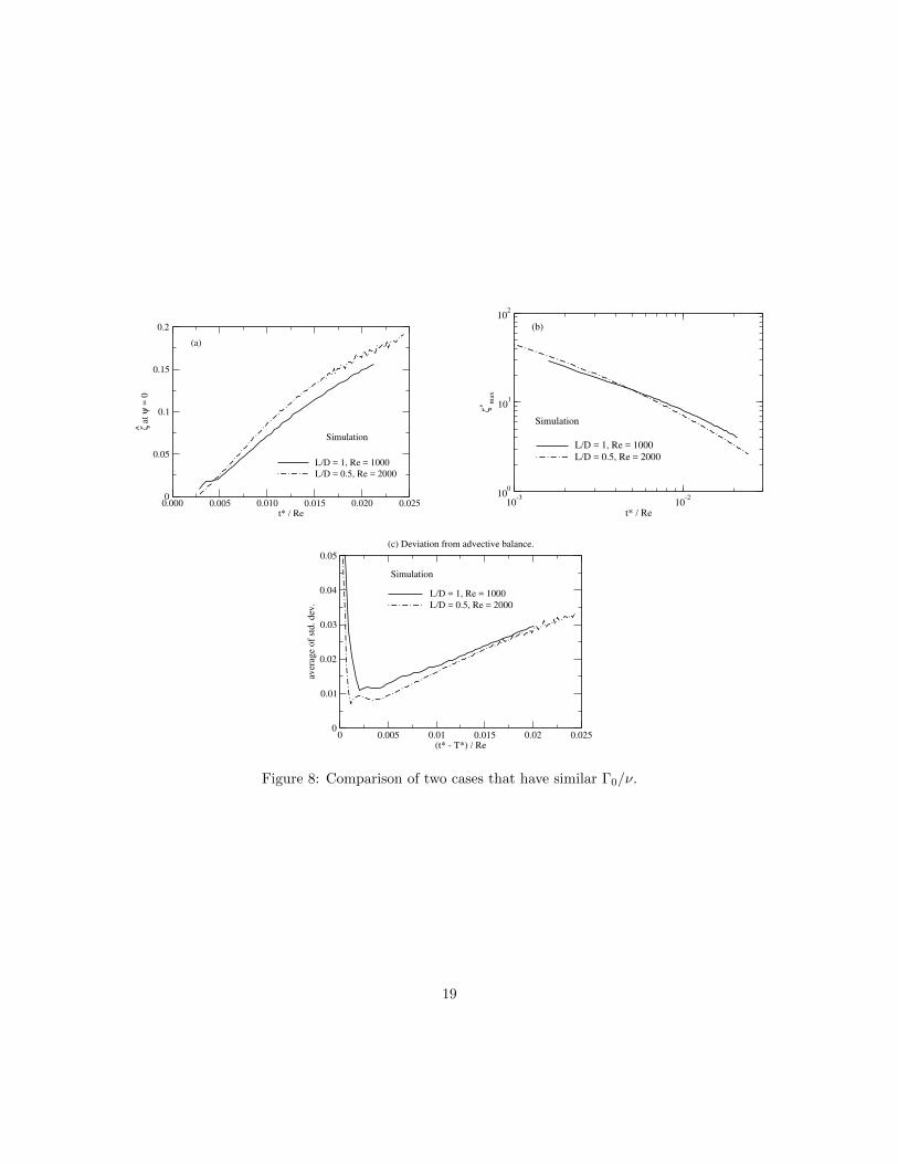
The notion that the L/D dependence is mostly due to changes in Γ0/ν can also be approximatelytested using the simulations in the following way. Substituting the expressions for piston stroke (5)and slug circulation (45) into the empirical equation (44) for Γ0 gives

Γ0/ν = .548ReL + 0.154Re, L/D ≤ (L/D)lim, (32)

where ReL ≡ U0L/ν is the Reynolds number based on piston stroke. Equation (32) shows thatmatching ReL approximately matches Γ0/ν. In particular, the two cases (Re = 2000, L/D = 0.5)and (Re = 1000, L/D = 1) have the same ReL = 1000 and (32) gives their corresponding Γ0/νas 856 and 702, respectively. Simulation results for the two cases are shown as the chain-dottedand solid black lines in Figure 8. Comparing them, one observes a reasonable correspondence inζ(ψ → 1−), ζ∗max, and the rate of loss of advective balance. The quantity ψ∗max is not shown; itcannot be expected to correspond in the two cases since it is affected by the core size to radiusratio.

18

0.000 0.005 0.010 0.015 0.020 0.025t* / Re

0

0.05

0.1

0.15

0.2

ζ^ a

t ψ

= 0

L/D = 1, Re = 1000

L/D = 0.5, Re = 2000

Simulation

(a)

10-3

10-2

t* / Re

100

101

102

ζ∗

max

L/D = 1, Re = 1000

L/D = 0.5, Re = 2000

Simulation

(b)

0 0.005 0.01 0.015 0.02 0.025(t* - T*) / Re

0

0.01

0.02

0.03

0.04

0.05

aver

age

of

std

. d

ev.

L/D = 1, Re = 1000

L/D = 0.5, Re = 2000

(c) Deviation from advective balance.

Simulation

Figure 8: Comparison of two cases that have similar Γ0/ν.

19

7 Summary

1. After a period of relaxation, a state of approximate advective balance, ζ ≈ ζ(ψ, t), is achievedwithin the region bounded by the dividing streamline.

2. The function ζ = ζ(ψ, t) (where hats denotes quantities normalized by peak values) evolvesin time from being convex to being approximately linear, but with a non-zero intercept as thedividing streamline is approached.

3. Introduction of the viscous time, t∗/Re = νt/D2, captures some but not all of the Reynolds

number dependence in the evolution of ζ = ζ(ψ, t). In particular, the value of ζ at thedividing streamline exhibits a strong extra Reynolds number dependence. To explain this,a toy vorticity diffusion model with an edge layer at the boundary was developed. Themodel indicates that the extra Reynolds number dependence arises primarily from role of νin determining the thickness of the edge layer. The dependence on L/D at later times arisesmostly from the ring Reynolds number Γ(t)/ν which determines the thickness of the edgelayer. The conventional Gaussian profile, in which ν enters (mostly) through the product νt,does not exhibit the extra Re dependence.

4. A diagnostic of the function ζ = ζ(ψ, t) was provided by the coefficients of its cubic fitplotted versus t∗/Re. They indicate a lessening with time (t∗/Re) of the L/D and (extra)Re dependence. Nevertheless, a non-negligible dependence on both parameters continues toremain, most prominently in the value of ζ as the dividing streamline is approached, for aslong as we have run the simulations.

8 Suggestions for future work

1. An important remaining question is how advective balance is maintained in the face of adiffusion term that acts to destroy it. Suppose that at some instant we have ζ = F (ψ, t),Then upon using the chain rule relations

∂F

∂x= −urr

∂F

∂ψ,

∂F

∂r= uxr

∂F

∂ψ, (33)

∂2F

∂x2= (urr)

2 ∂2F

∂ψ2− r ∂ur

∂x

∂F

∂ψ, (34)

∂2F

∂r2= (uxr)

2 ∂2F

∂ψ2+∂(uxr)

∂r

∂F

∂ψ, (35)

together with

ζ =ωφr

=1

r

(∂ur∂x− ∂ux

∂r

), (36)

the vorticity equation (3) becomes:

∂F

∂τ= r2q2 ∂

2F

∂ψ2−(r2F − 4ux

) ∂F∂ψ

, (37)

where τ = νt and q2 = u2x+u2

r. The coefficients r2q2, r2, and ux of the three terms on the right-hand-side of (37) are not functions of ψ only. This should be contrasted with the planar case

20

where streamlines are circular and the diffusion operator is a function of ψ2D. We concludethat the diffusion term in axisymmetric flow acts to destroy advective balance. How is itthen restored? A reasonable conjecture is that disturbances to the advectively-balanced stateinduced by the diffusion term are sheared by differential rotation and eventually average outalong each closed streamline. Note that this is an advective effect. It is analogous to averagingby Taylor (or shear) dispersion of a passive scalar around closed streamlines studied for planarflow by Rhines & Young (1983), who conjectured that the same mechanism could occur forvorticity. When the Reynolds number, Γ(t)/ν, becomes sufficiently small, destruction ofadvective balance by the diffusion term will dominate its restoration by differential rotation.

2. If streamline-averaging accurately describes the restoring effect of advection, then the follow-ing algorithm could be used to compute the evolution of ζ: (i) Diffuse ζ for a short timeδt imposing the boundary condition dictated by the edge layer. (ii) To mimic the effect ofadvection, average ζ along each closed streamline. Upon combining the two steps into one,(37) becomes

∂F

∂τ=⟨r2q2

⟩ ∂2F

∂ψ2−(⟨r2⟩F − 4 〈ux〉

) ∂F∂ψ

, (38)

within the vortex ring bubble. Here 〈.〉 denotes an average around a closed streamline. (iii)The final step of the algorithm would be to compute the resulting velocity field and stream-function from the Poisson equation.

3. The most non-trivial aspect of the above procedure is obtaining the boundary condition onF (ψ) where the flow in the interior of the bubble matches with edge layers. The presentwork ignored the detailed structure of the edge layer and wake. They should be studied inthe future. Hints can be obtained from the work of Harper & Moore (1968) on falling drops.An analytical or semi-analytical treatment that matches the interior flow, edge layers, andexterior potential flow would be most satisfying. An even more satisfying analysis would alsoquantify the deviation from advective balance at every location around a closed streamline.One aspect of this deviation is the forward lean of vorticity contours seen in Figure 2a (Prof.Brian Cantwell, private communication). This fore-aft asymmetry may be related to thefact that the windward side of the edge-layer experiences positive strain along the dividingstreamline, while the opposite is true on the leeward side.

4. The Prandtl-Batchelor theorem asserts that F (ψ) = constant for exactly steady axisymmetricflow with closed streamlines (Batchelor, 1956, pp. 186-187), a result obtained by integratingthe momentum equation around a closed streamline. The critical assumption is that therate of change of circulation around every closed streamline is zero. Even though this is nottrue in the present case, Batchelor’s integral analysis might still be useful. Note that therecirculation region of a wake behind an axisymmetric bluff body or the interior of a fallingdrop (Harper & Moore, 1968) can remain steady, in spite of viscous diffusion, because of acontinual source of vorticity at the dividing streamline. For a bluff body, this source is theseparated boundary-layer of the body, and for a drop it is the boundary condition of stressand velocity continuity at the two-fluid interface. In the present situation, there is a sink ofvorticity at the dividing streamline.

AcknowledgementsKS is grateful to Thomas Hartlep and Alan Wray for their suggestions during the internal

review. We also thank the referees for their useful suggestions.

21

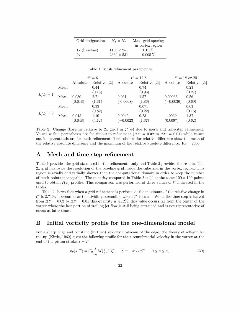
Grid designation Nx ×Nr Max. grid spacingin vortex region

1x (baseline) 1103× 251 0.01D2x 2339× 531 0.005D

Table 1: Mesh refinement parameters.

t∗ = 6 t∗ = 12.8 t∗ = 18 or 20Absolute Relative [%] Absolute Relative [%] Absolute Relative [%]

L/D = 1

Mean 0.44 0.74 0.23(0.15) (0.93) (0.27)

Max. 0.030 2.71 0.031 1.57 0.00063 0.56(0.018) (1.31) (-0.0068) (1.86) (−0.0030) (0.69)

L/D = 3

Mean 0.33 0.071 0.63(0.82) (0.22) (0.16)

Max. 0.015 1.19 0.0042 0.23 −.0069 1.37(0.048) (4.12) (−0.0023) (1.37) (0.0097) (0.62)

Table 2: Change (baseline relative to 2x grid) in ζ∗(ψ) due to mesh and time-step refinement.Values within parentheses are for time-step refinement (∆t∗ = 0.02 to ∆t∗ = 0.01) while valuesoutside parenthesis are for mesh refinement. The columns for relative difference show the mean ofthe relative absolute difference and the maximum of the relative absolute difference. Re = 2000.

A Mesh and time-step refinement

Table 1 provides the grid sizes used in the refinement study and Table 2 provides the results. The2x grid has twice the resolution of the baseline grid inside the tube and in the vortex region. Thisregion is axially and radially shorter than the computational domain in order to keep the numberof mesh points manageable. The quantity compared in Table 2 is ζ∗ at the same 100× 100 pointsused to obtain ζ(ψ) profiles. This comparison was performed at three values of t∗ indicated in thetables.

Table 2 shows that when a grid refinement is performed, the maximum of the relative change inζ∗ is 2.71%; it occurs near the dividing streamline where ζ∗ is small. When the time step is halvedfrom ∆t∗ = 0.02 to ∆t∗ = 0.01 this quantity is 4.12%; this value occurs far from the center of thevortex where the last portion of trailing jet flow is still being entrained and is not representative oferrors at later times.

B Initial vorticity profile for the one-dimensional model

For a sharp edge and constant (in time) velocity upstream of the edge, the theory of self-similarroll-up (Kirde, 1962) gives the following profile for the circumferential velocity in the vortex at theend of the piston stroke, t = T :

uθ(s, T ) = C0s

s0M( 3

4 , 2; ξ), ξ ≡ −s2/4νT, 0 ≤ s ≤ s0, (39)

22

where s is cylindrical radial distance from the core center, s0 is the outermost radius of the vortexspiral at t = T , and M(a, b;x) is the confluent hypergeometric function (Abramowitz & Stegun,1965, p. 503), and the constant C0 is

C0 = uθ(s0)[M( 3

4 , 2; ξ0)]−1

, ξ0 ≡ −s20/4νT. (40)

The diffusion model of the paper requires specification of the vorticity corresponding to (39) whichis

ωφ(s, T ) =1

s

∂

∂s(suθ) =

C0

s0

[2M( 3

4 , 2; ξ) +3

4ξM( 7

4 , 3; ξ)

], 0 ≤ s ≤ s0, (41)

with ωφ = 0 for s > s0. Kirde’s theory does not consider the profile in the outer region of the core,denoted as region I in Pullin (1979); in terminating the velocity profile (39) at s = s0 and settingωφ = 0 for s > s0, we are following equation (2.16) in Saffman (1978).

To specify the radius, s0, of the vortex spiral and the initial ring radius, R0, we use the followingexpressions from Saffman (1978):

(s0)Saffman = 0.28D1/3L2/3, R0 = D/2 + 0.11D1/3L2/3, (42)

which use scalings from the theory of self-similar roll-up and constants from fitting experiments.For the 0.28 constant, see the fourth line after Saffman’s eq. 3.6, and for the 0.11 constant seethe second line on pg. 633 of Saffman’s paper. To prevent the spiral from over-filling the notionaldividing streamline, we set s0 = min [(s0)Saffman, sDS].

The circumferential velocity at the core boundary is obtained from the circulation, i.e.,

uθ(s0) = Γ0/2πs0, (43)

where for the circulation Γ0 we use

Γ0

Γslug= 1.14 + 0.32(L/D)−1, (44)

which is equation (2.6) from Shariff & Leonard (1992) and represents a fit to experiments. For thetrapezoidal piston velocity prescribed in the present work, the slug circulation is

Γslug ≡1

2

∫ T

0

U2p(t) dt = 0.433U2

0T. (45)

References

Abramowitz, M. & Stegun, I.A. 1965 Handbook of Mathematical Functions. New York: Dover.

Batchelor, G.K. 1956 On steady laminar flow with closed streamlines at large Reynolds number.J. Fluid Mech. 1, 177–190.

Batchelor, G.K. 1967 An Introduction to Fluid Dynamics. Cambridge University Press.

Berezovski, A.A. & Kaplanski, F.B. 1987 Diffusion of a ring vortex. Fluid Dyn. 22 (6), 832–837, Transl. of Izvestiya Akademii Nauk, Mekhanika Zhidkosti i Gaza.

23

Cater, J.E., Soria, J. & Lim, T. T. 2004 The interaction of the piston vortex with a piston-generated vortex ring. J. Fluid Mech. 499, 327–343.

Couder, Y. & Basdevant, C. 1986 Experimental and numerical study of vortex couples intwo-dimensional flows. J. Fluid Mech. 173, 225–251.

Eydeland, A. & Turkington, B. 1988 A computational method of solving free-boundary prob-lems in vortex dynamics. J. Comp. Phys. 78, 194–214.

Ferziger, J.H. & Peric, M. 2002 Computational Methods for Fluid Dynamics. Berlin: Springer.

Fukumoto, Y. & Moffatt, H. K. 2000 Motion and expansion of a viscous vortex ring. Part 1.A higher-order asymptotic formula for the velocity. J. Fluid Mech. 417, 1–45.

Gharib, M., Rambod, E. & Shariff, K. 1998 A universal time scale for vortex ring formation.J. Fluid Mech. 360, 121–140.

Harper, J. F. & Moore, D. W. 1968 The motion of a spherical liquid drop at high Reynoldsnumber. J. Fluid Mech. 32 (2), 367–391.

Kambe, T. & Oshima, Y. 1975 Generation and decay of viscous vortex rings. J. Phys. Soc. ofJapan 38 (1), 271–280.

Kaplanski, F., Fukumoto, Y. & Rudi, Y. 2012 Reynolds-number effect on vortex ring evolutionin a viscous fluid. Phys. Fluids 24 (3), 033101:1–13.

Kaplanski, F.B. & Rudi, Y.A. 2001 Evolution of a viscous vortex ring. Fluid Dyn. 36 (1), 16–25,Transl. of Izvestiya Akademii Nauk, Mekhanika Zhidkosti i Gaza.

Kaplanski, F.B. & Rudi, Y.A. 2005 A model for the formation of “optimal” rings taking intoaccount viscosity. Phys. Fluids 17, 087101:1–7.

Kirde, K. 1962 Untersuchungen uber die zeitliche Weiterentwicklung eines Wirbels mitVorgegebener Anfangsverteilung. Ingenieur-Archiv 31 (6), 385–404.

Leonard, B.P. 1979 A stable and accurate convective modelling procedure based on quadraticupstream interpolation. Computer Meth. Appl. Mech. Engr. 19, 59–98.

Linden, P.F. & Turner, J.S. 2001 The formation of ‘optimal’ vortex rings and the efficiency ofpropulsive devices. J. Fluid Mech. 427, 61–72.

Mohseni, K. & Gharib, M. 1998 A model for universal time scale of vortex ring formation. Phys.Fluids 10, 2436–2438.

Moore, D. W. 1980 The velocity of a vortex ring with a thin core of elliptical cross section. Proc.Roy. Soc. Lond. A 370 (1742), 407–415.

Nitsche, M. & Krasny, R. 1994 A numerical study of vortex ring formation at the edge of acircular tube. J. Fluid Mech. 276, 139–161.

Norbury, J. 1973 A family of steady vortex rings. J. Fluid Mech. 57, 417–431.

24

Phillips, O. M. 1956 The final period of decay of non-homogeneous turbulence. Math. Proc.Cambridge Phil. Soc. 52 (1), 135–151.

Pullin, D. 1979 Vortex ring formation at tube and orifice openings. Phys. Fluids 22 (3), 401–403.

Rhines, P.B. & Young, W.R. 1983 How rapidly is a passive scalar mixed within closed stream-lines? J. Fluid Mech. 133, 133–145.

Rott, N. & Cantwell, B. 1993a Vortex drift. I: Dynamic interpretation. Phys. Fluids A 5 (6),1443–1450.

Rott, N. & Cantwell, B. 1993b Vortex drift. II: The flow potential surrounding a driftingvortical region. Phys. Fluids A 5 (6), 1451–1455.

Saffman, P. G. 1970 The velocity of viscous vortex rings. Stud. Appl. Math. 49 (4), 371–380.

Saffman, P. G. 1978 The number of waves on unstable vortex rings. J. Fluid Mech. 84 (4),625–639.

Shariff, K. & Leonard, A. 1992 Vortex rings. Ann. Rev. Fluid Mech. 24, 235–279.

Shusser, M. & Gharib, M. 2000 Energy and velocity of a forming vortex ring. Phys. Fluids12 (3), 618–621.

Stanaway, S., Cantwell, B.J. & Spalart, P.R. 1988 A numerical study of viscous vortexrings using a spectral method. Technical Memorandum 101041. NASA.

25