Advanced Regression Summer Statistics Institute · Regression Model Assumptions Y i = 0 + 1X i +...
80
Advanced Regression Summer Statistics Institute Day 3: Transformations and Non-Linear Models 1
Transcript of Advanced Regression Summer Statistics Institute · Regression Model Assumptions Y i = 0 + 1X i +...
Advanced RegressionSummer Statistics Institute
Day 3: Transformations and Non-Linear Models
1
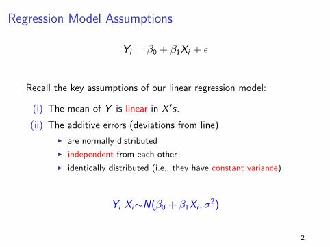
Regression Model Assumptions
Yi = β0 + β1Xi + ε
Recall the key assumptions of our linear regression model:
(i) The mean of Y is linear in X ′s.
(ii) The additive errors (deviations from line)
I are normally distributed
I independent from each other
I identically distributed (i.e., they have constant variance)
Yi |Xi∼N(β0 + β1Xi , σ2)
2
Regression Model Assumptions
Inference and prediction relies on this model being “true”!
If the model assumptions do not hold, then all bets are off:
I prediction can be systematically biased
I standard errors, intervals, and t-tests are wrong
We will focus on using graphical methods (plots!) to detect
violations of the model assumptions.
3
Example
4 6 8 10 12 14
456789
11
x1
y1
4 6 8 10 12 14
34
56
78
9
x2
y2
4 6 8 10 12 14
68
10
12
x3
y3
8 10 12 14 16 18
68
10
12
x4
y4
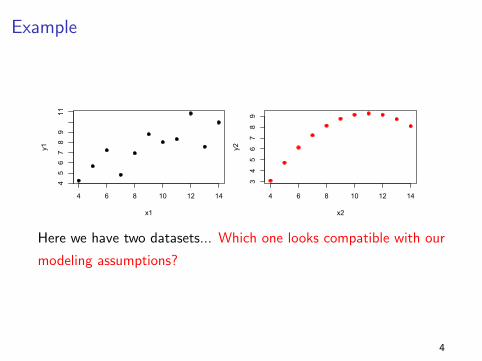
Here we have two datasets... Which one looks compatible with our
modeling assumptions?
4
Example
Week VII. Slide 13Applied Regression Analysis Carlos M. Carvalho
(1)
(2)
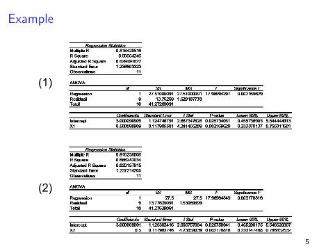
Example where things can go bad!
5
Example
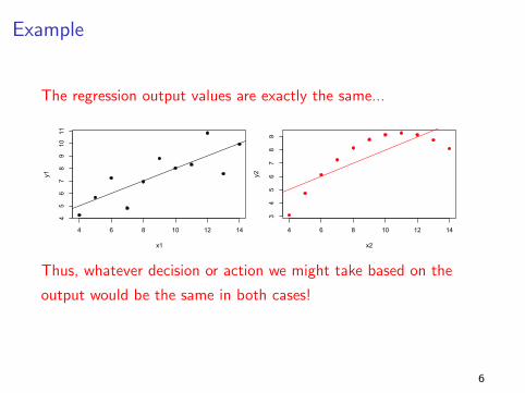
The regression output values are exactly the same...
4 6 8 10 12 14
45
67
89
1011
x1
y1
4 6 8 10 12 14
34
56
78
9
x2
y2
4 6 8 10 12 14
68
10
12
x3
y3
8 10 12 14 16 18
68
10
12
x4
y4
Thus, whatever decision or action we might take based on the
output would be the same in both cases!
6
Example
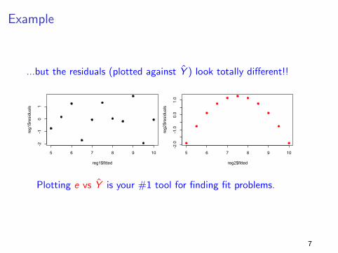
...but the residuals (plotted against Y ) look totally different!!
5 6 7 8 9 10
-2-1
01
reg1$fitted
reg1$residuals
5 6 7 8 9 10
-2.0
-1.0
0.0
1.0
reg2$fittedreg2$residuals
5 6 7 8 9 10
-10
12
3
reg3$fitted
reg3$residuals
7 8 9 10 11 12
-1.5
-0.5
0.5
1.5
reg4$fitted
reg4$residualsPlotting e vs Y is your #1 tool for finding fit problems.
7
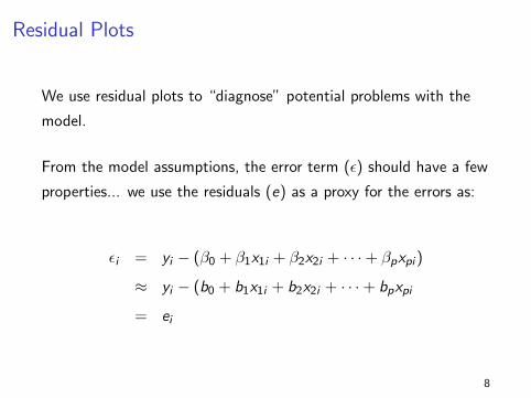
Residual Plots
We use residual plots to “diagnose” potential problems with the
model.
From the model assumptions, the error term (ε) should have a few
properties... we use the residuals (e) as a proxy for the errors as:
εi = yi − (β0 + β1x1i + β2x2i + · · ·+ βpxpi )
≈ yi − (b0 + b1x1i + b2x2i + · · ·+ bpxpi
= ei
8
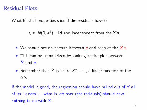
Residual Plots
What kind of properties should the residuals have??
ei ≈ N(0, σ2) iid and independent from the X’s
I We should see no pattern between e and each of the X ’s
I This can be summarized by looking at the plot between
Y and e
I Remember that Y is “pure X”, i.e., a linear function of the
X ’s.
If the model is good, the regression should have pulled out of Y all
of its “x ness”... what is left over (the residuals) should have
nothing to do with X .9
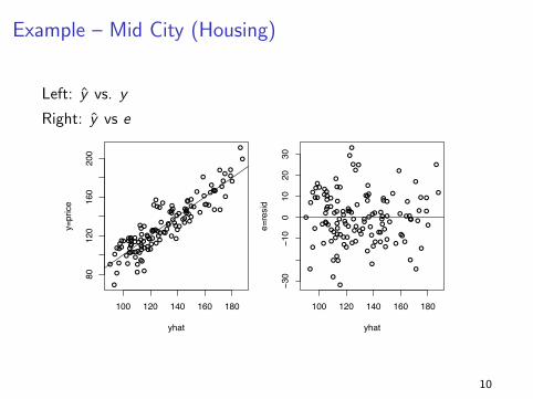
Example – Mid City (Housing)
Left: y vs. y
Right: y vs e
Example, the midcity housing regression:
Left: y vs fits, Right: fits vs. resids (y vs. e).
! !!
!
!!
!!
!
!
!
!
!
!
!
! !
!
!
!
!!
!
!
!
!
!
!
!
!!
!
!!
! !!
!
!
!!
!
!
!
!
!
!
!
!
!
!
!
!
!
!
!
!
!
!
!
!
!
!
!
!
!
!
!
!
! !
!
!
!
!
!
!
!
!
! !
!
!
!
!
!
!
!
!
!
!
!
!
!!
!
!!
!
!
!
!
!
!
!
!
!
!
!
!!!
!
!
!
!
!
!
!
! !!
!
!
!
!
!
!
100 120 140 160 180
80120
160
200
yhat
y=price !
!
!
!
!
!
!
!!
!
!
!!
!
!
!
!
!
!
!
!
!
!
!
!
!
!
!
!
!
!
!!
!
!
!
!
!
!
!!
!
!
!
!!
!
!
!
!
!
!
!
!
!
!!
!!
!
!
!
!!
!
!!
!
!
!
!
!
!
!
!
!
!
!
! !
!
!
!
!
!
!
!
!
!
!
!
!!
!
!
!
!!
! !
!!
!
!
!
!
!
!
!
!
!!
!
!
!
!
!!
!
!
!
!
!
!
!!
!!
100 120 140 160 180
−30
−10
010
2030
yhat
e=resid
10
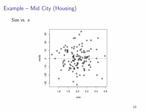
Example – Mid City (Housing)
Size vs. ex= size of house vs. resids for midcity multiple regression.
!
!
!
!
!
!
!
!!
!
!
!!
!
!
!
!
!
!
!
!
!
!
!
!
!
!
!
!
!
!
!!
!
!
!
!
!
!
!!
!
!
!
!
!
!
!
!
!
!
!
!
!
!
!
!
!!
!
!
!
!!
!
!
!
!
!
!
!
!
!
!
!
!
!
!
!!
!
!
!
!
!
!
!
!
!
!
!
!
!
!
!
!
!!
!!
!!
!
!
!
!
!
!
!
!
!!
!
!
!
!
!!
!
!
!
!
!
!
!!
!!
1.6 1.8 2.0 2.2 2.4 2.6
−30
−20
−10
010
2030
size
resids
11
Example – Mid City (Housing)
I In the Mid City housing example, the residuals plots (both X
vs. e and Y vs. e) showed no obvious problem...
I This is what we want!!
I Although these plots don’t guarantee that all is well it is a
very good sign that the model is doing a good job.
12
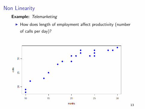
Non Linearity
Example: Telemarketing
I How does length of employment affect productivity (number
of calls per day)?
13
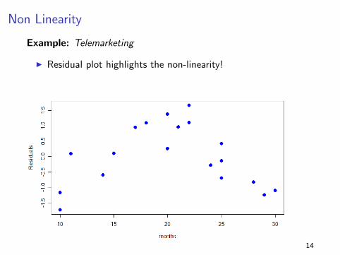
Non Linearity
Example: Telemarketing
I Residual plot highlights the non-linearity!
14
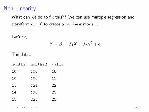
Non Linearity
What can we do to fix this?? We can use multiple regression and
transform our X to create a no linear model...
Let’s try
Y = β0 + β1X + β2X2 + ε
The data...
months months2 calls
10 100 18
10 100 19
11 121 22
14 196 23
15 225 25
... ... ... 15
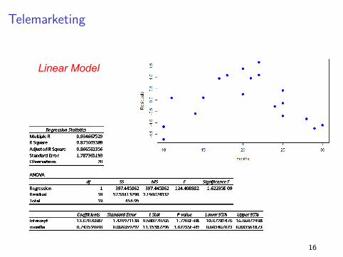
TelemarketingAdding Polynomials
Week VIII. Slide 5Applied Regression Analysis Carlos M. Carvalho
Linear Model
16
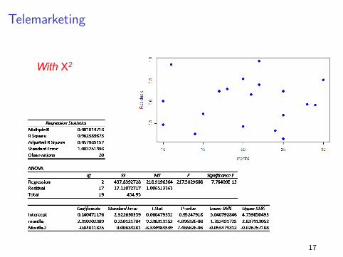
TelemarketingAdding Polynomials
Week VIII. Slide 6Applied Regression Analysis Carlos M. Carvalho
With X2
17
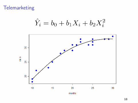
TelemarketingAdding Polynomials
Week VIII. Slide 7Applied Regression Analysis Carlos M. Carvalho
18
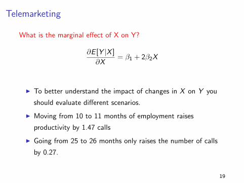
Telemarketing
What is the marginal effect of X on Y?
∂E [Y |X ]
∂X= β1 + 2β2X
I To better understand the impact of changes in X on Y you
should evaluate different scenarios.
I Moving from 10 to 11 months of employment raises
productivity by 1.47 calls
I Going from 25 to 26 months only raises the number of calls
by 0.27.
19
Polynomial Regression
Even though we are limited to a linear mean, it is possible to get
nonlinear regression by transforming the X variable.
In general, we can add powers of X to get polynomial regression:
Y = β0 + β1X + β2X2 . . .+ βmXm
You can fit any mean function if m is big enough.
Usually, m = 2 does the trick.
20
Closing Comments on Polynomials
We can always add higher powers (cubic, etc) if necessary.
Be very careful about predicting outside the data range. The curve
may do unintended things beyond the observed data.
Watch out for over-fitting... remember, simple models are
“better”.
21
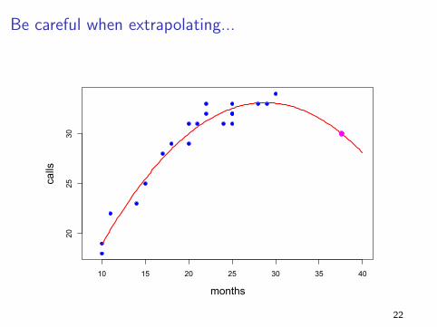
Be careful when extrapolating...
10 15 20 25 30 35 40
2025
30
months
calls
22
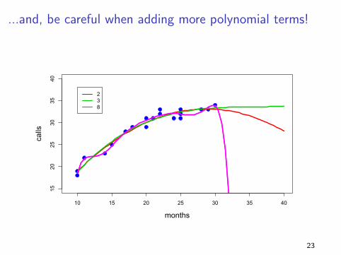
...and, be careful when adding more polynomial terms!
10 15 20 25 30 35 40
1520
2530
3540
months
calls
238
23
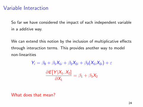
Variable Interaction
So far we have considered the impact of each independent variable
in a additive way.
We can extend this notion by the inclusion of multiplicative effects
through interaction terms. This provides another way to model
non-linearities
Yi = β0 + β1X1i + β2X2i + β3(X1iX2i) + ε
∂E [Y |X1,X2]
∂X1= β1 + β3X2
What does that mean?
24
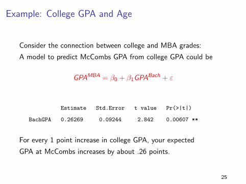
Example: College GPA and Age
Consider the connection between college and MBA grades:
A model to predict McCombs GPA from college GPA could be
GPAMBA = β0 + β1GPABach + ε
Estimate Std.Error t value Pr(>|t|)
BachGPA 0.26269 0.09244 2.842 0.00607 **
For every 1 point increase in college GPA, your expected
GPA at McCombs increases by about .26 points.
25
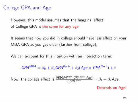
College GPA and Age
However, this model assumes that the marginal effect
of College GPA is the same for any age.
It seems that how you did in college should have less effect on your
MBA GPA as you get older (farther from college).
We can account for this intuition with an interaction term:
GPAMBA = β0 + β1GPABach + β2(Age × GPABach) + ε
Now, the college effect is ∂E [GPAMBA|GPABach Age]∂GPABach = β1 + β2Age.
Depends on Age!
26
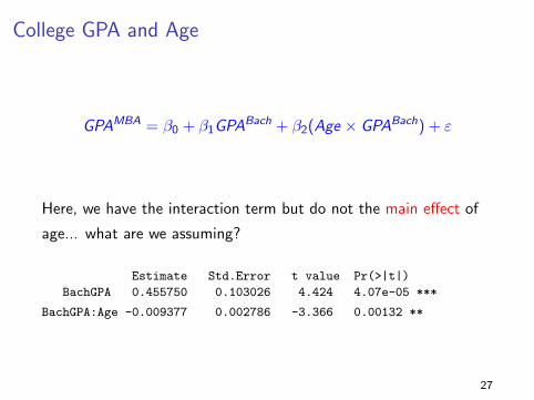
College GPA and Age
GPAMBA = β0 + β1GPABach + β2(Age × GPABach) + ε
Here, we have the interaction term but do not the main effect of
age... what are we assuming?
Estimate Std.Error t value Pr(>|t|)
BachGPA 0.455750 0.103026 4.424 4.07e-05 ***
BachGPA:Age -0.009377 0.002786 -3.366 0.00132 **
27
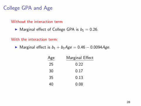
College GPA and Age
Without the interaction term
I Marginal effect of College GPA is b1 = 0.26.
With the interaction term:
I Marginal effect is b1 + b2Age = 0.46− 0.0094Age.
Age Marginal Effect
25 0.22
30 0.17
35 0.13
40 0.08
28

Non-constant Variance
Example...
This violates our assumption that all εi have the same σ2.
29
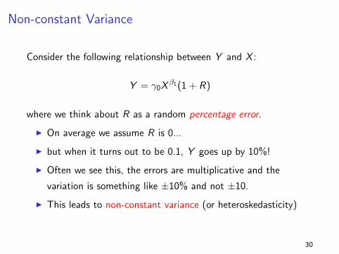
Non-constant Variance
Consider the following relationship between Y and X :
Y = γ0Xβ1(1 + R)
where we think about R as a random percentage error.
I On average we assume R is 0...
I but when it turns out to be 0.1, Y goes up by 10%!
I Often we see this, the errors are multiplicative and the
variation is something like ±10% and not ±10.
I This leads to non-constant variance (or heteroskedasticity)
30
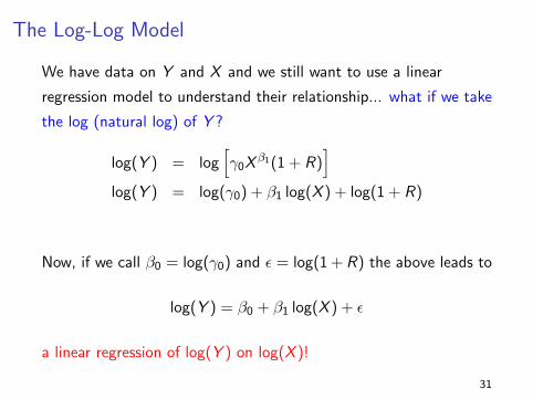
The Log-Log Model
We have data on Y and X and we still want to use a linear
regression model to understand their relationship... what if we take
the log (natural log) of Y ?
log(Y ) = log[γ0X
β1(1 + R)]
log(Y ) = log(γ0) + β1 log(X ) + log(1 + R)
Now, if we call β0 = log(γ0) and ε = log(1 + R) the above leads to
log(Y ) = β0 + β1 log(X ) + ε
a linear regression of log(Y ) on log(X )!
31

The Log-Log Model
Consider a country’s GDP as a function of IMPORTS :
I Since trade multiplies, we might expect to
see %GDP to increase with %IMPORTS .
0 200 400 600 800 1000 1200
02000
4000
6000
8000
10000
IMPORTS
GDP
ArgentinaAustraliaBolivia
BrazilCanada
CubaDenmarkEgyptFinland
France
GreeceHaiti
India
IsraelJamaica
Japan
LiberiaMalaysiaMauritiusNetherlandsNigeriaPanamaSamoa
United Kingdom
United States
-2 0 2 4 6 8
02
46
8
log(IMPORTS)
log(GDP)
ArgentinaAustralia
Bolivia
BrazilCanada
Cuba
DenmarkEgypt
Finland
France
Greece
Haiti
India
Israel
Jamaica
Japan
Liberia
Malaysia
Mauritius
Netherlands
Nigeria
Panama
Samoa
United Kingdom
United States
32
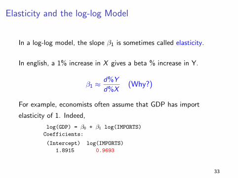
Elasticity and the log-log Model
In a log-log model, the slope β1 is sometimes called elasticity.
In english, a 1% increase in X gives a beta % increase in Y.
β1 ≈d%Y
d%X(Why?)
For example, economists often assume that GDP has import
elasticity of 1. Indeed,
log(GDP) = β0 + β1 log(IMPORTS)
Coefficients:
(Intercept) log(IMPORTS)
1.8915 0.9693
33
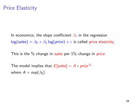
Price Elasticity
In economics, the slope coefficient β1 in the regression
log(sales) = β0 + β1 log(price) + ε is called price elasticity.
This is the % change in sales per 1% change in price.
The model implies that E [sales] = A ∗ priceβ1
where A = exp(β0)
34
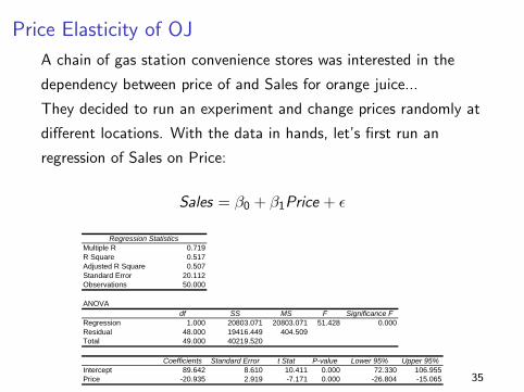
Price Elasticity of OJ
A chain of gas station convenience stores was interested in the
dependency between price of and Sales for orange juice...
They decided to run an experiment and change prices randomly at
different locations. With the data in hands, let’s first run an
regression of Sales on Price:
Sales = β0 + β1Price + εSUMMARY OUTPUT
Regression StatisticsMultiple R 0.719R Square 0.517Adjusted R Square 0.507Standard Error 20.112Observations 50.000
ANOVAdf SS MS F Significance F
Regression 1.000 20803.071 20803.071 51.428 0.000Residual 48.000 19416.449 404.509Total 49.000 40219.520
Coefficients Standard Error t Stat P-value Lower 95% Upper 95%Intercept 89.642 8.610 10.411 0.000 72.330 106.955Price -20.935 2.919 -7.171 0.000 -26.804 -15.065 35
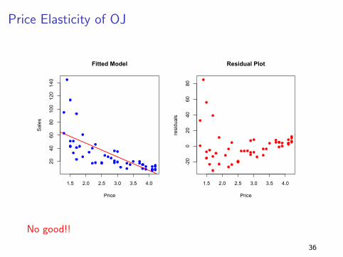
Price Elasticity of OJ
1.5 2.0 2.5 3.0 3.5 4.0
2040
6080
100120140
Fitted Model
Price
Sales
1.5 2.0 2.5 3.0 3.5 4.0-20
020
4060
80
Residual Plot
Price
residuals
No good!!
36
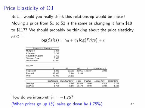
Price Elasticity of OJ
But... would you really think this relationship would be linear?
Moving a price from $1 to $2 is the same as changing it form $10
to $11?? We should probably be thinking about the price elasticity
of OJ...log(Sales) = γ0 + γ1 log(Price) + ε
SUMMARY OUTPUT
Regression StatisticsMultiple R 0.869R Square 0.755Adjusted R Square 0.750Standard Error 0.386Observations 50.000
ANOVAdf SS MS F Significance F
Regression 1.000 22.055 22.055 148.187 0.000Residual 48.000 7.144 0.149Total 49.000 29.199
Coefficients Standard Error t Stat P-value Lower 95% Upper 95%Intercept 4.812 0.148 32.504 0.000 4.514 5.109LogPrice -1.752 0.144 -12.173 0.000 -2.042 -1.463
How do we interpret γ1 = −1.75?
(When prices go up 1%, sales go down by 1.75%) 37
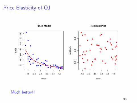
Price Elasticity of OJ
1.5 2.0 2.5 3.0 3.5 4.0
2040
6080
100120140
Fitted Model
Price
Sales
1.5 2.0 2.5 3.0 3.5 4.0-0.5
0.0
0.5
Residual Plot
Price
residuals
Much better!!
38
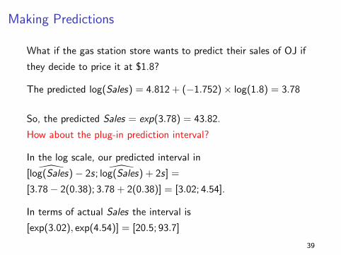
Making Predictions
What if the gas station store wants to predict their sales of OJ if
they decide to price it at $1.8?
The predicted log(Sales) = 4.812 + (−1.752)× log(1.8) = 3.78
So, the predicted Sales = exp(3.78) = 43.82.
How about the plug-in prediction interval?
In the log scale, our predicted interval in
[ log(Sales)− 2s; log(Sales) + 2s] =
[3.78− 2(0.38); 3.78 + 2(0.38)] = [3.02; 4.54].
In terms of actual Sales the interval is
[exp(3.02), exp(4.54)] = [20.5; 93.7]
39
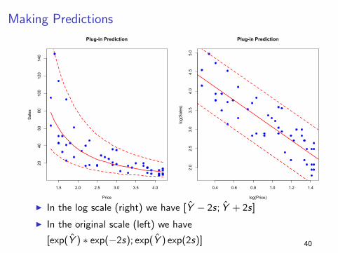
Making Predictions
1.5 2.0 2.5 3.0 3.5 4.0
2040
6080
100
120
140
Plug-in Prediction
Price
Sales
0.4 0.6 0.8 1.0 1.2 1.42.0
2.5
3.0
3.5
4.0
4.5
5.0
Plug-in Prediction
log(Price)
log(Sales)
I In the log scale (right) we have [Y − 2s; Y + 2s]
I In the original scale (left) we have
[exp(Y ) ∗ exp(−2s); exp(Y ) exp(2s)] 40
Some additional comments...
I Another useful transformation to deal with non-constant
variance is to take only the log(Y ) and keep X the same.
Clearly the “elasticity” interpretation no longer holds.
I Always be careful in interpreting the models after a
transformation
I Also, be careful in using the transformed model to make
predictions
41
Summary of Transformations
Coming up with a good regression model is usually an iterative
procedure. Use plots of residuals vs X or Y to determine the next
step.
Log transform is your best friend when dealing with non-constant
variance (log(X ), log(Y ), or both).
Add polynomial terms (e.g. X 2) to get nonlinear regression.
The bottom line: you should combine what the plots and the
regression output are telling you with your common sense and
knowledge about the problem. Keep playing around with it until
you get something that makes sense and has nothing obviously
wrong with it. 42
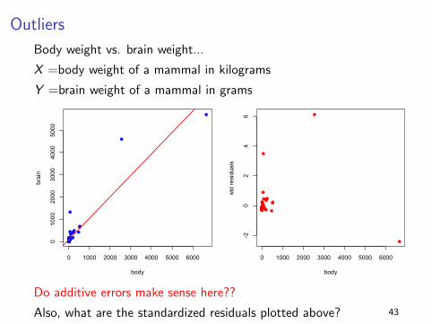
Outliers
Body weight vs. brain weight...
X =body weight of a mammal in kilograms
Y =brain weight of a mammal in grams
0 1000 2000 3000 4000 5000 6000
01000
2000
3000
4000
5000
body
brain
0 1000 2000 3000 4000 5000 6000
-20
24
6
body
std
resi
dual
s
Do additive errors make sense here??
Also, what are the standardized residuals plotted above? 43
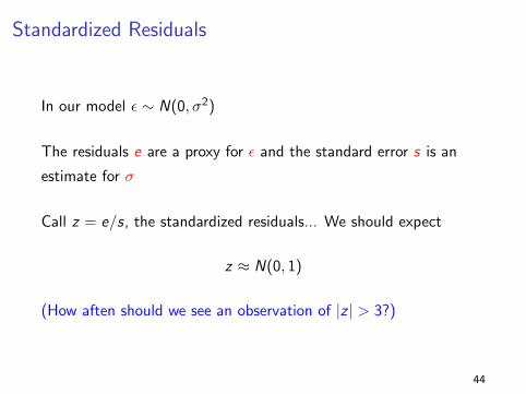
Standardized Residuals
In our model ε ∼ N(0, σ2)
The residuals e are a proxy for ε and the standard error s is an
estimate for σ
Call z = e/s, the standardized residuals... We should expect
z ≈ N(0, 1)
(How aften should we see an observation of |z | > 3?)
44
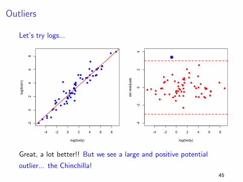
Outliers
Let’s try logs...
-4 -2 0 2 4 6 8
-20
24
68
log(body)
log(brain)
-4 -2 0 2 4 6 8
-4-2
02
4log(body)
std
resi
dual
s
Great, a lot better!! But we see a large and positive potential
outlier... the Chinchilla!45
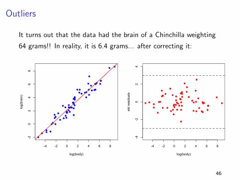
Outliers
It turns out that the data had the brain of a Chinchilla weighting
64 grams!! In reality, it is 6.4 grams... after correcting it:
-4 -2 0 2 4 6 8
-20
24
68
log(body)
log(brain)
-4 -2 0 2 4 6 8
-4-2
02
4
log(body)
std
resi
dual
s
46
How to Deal with Outliers
When should you delete outliers?
Only when you have a really good reason!
There is nothing wrong with running regression with and without
potential outliers to see whether results are significantly impacted.
Any time outliers are dropped the reasons for
removing observations should be clearly noted.
47
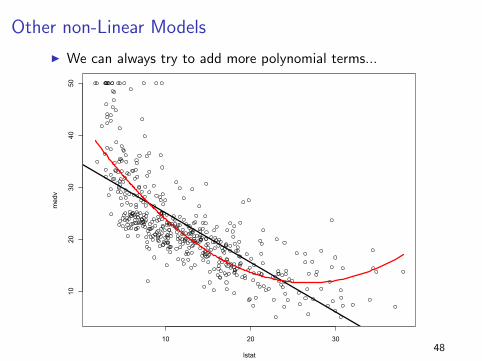
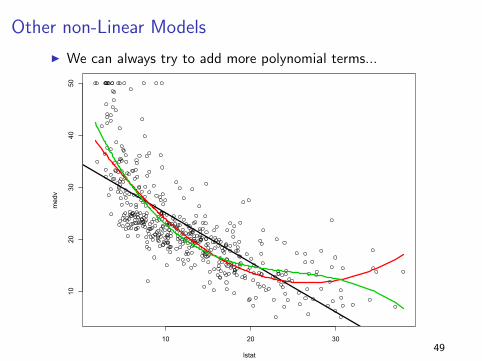
Other non-Linear Models
I We can always try to add more polynomial terms...
10 20 30
1020
3040
50
lstat
medv
48
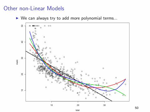
Other non-Linear Models
I We can always try to add more polynomial terms...
10 20 30
1020
3040
50
lstat
medv
49
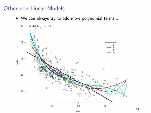
Other non-Linear Models
I We can always try to add more polynomial terms...
10 20 30
1020
3040
50
lstat
medv
50
Other non-Linear Models
I We can always try to add more polynomial terms...
10 20 30
1020
3040
50
lstat
medv
23415
51
Other non-Linear Models
I Or use a different set of “Basis Function”
Yi = β0 + β1b1(Xi ) + β2b2(Xi ) + · · ·+ βpbp(Xi ) + εi
I Notice that this has a form of a linear model and can,
therefore, be estimated via LS.
I There are a million different choices of bases... we’ll focus on
the most popular one: Splines
52
Regression Splines
I A spline works by fitting different low dimensional polynomials
over different regions of the predictor space
I The points where the coefficients change are called knots
I The more knots you use, the more flexibility you have (but
also more complexity!)
53
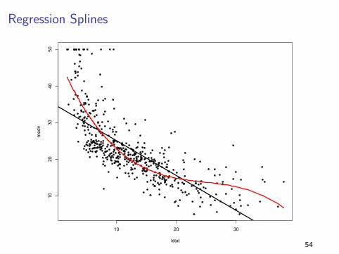
Regression Splines
10 20 30
1020
3040
50
lstat
medv
54
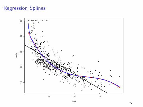
Regression Splines
10 20 30
1020
3040
50
lstat
medv
55
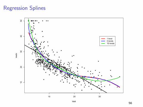
Regression Splines
10 20 30
1020
3040
50
lstat
medv
1 knot3 knots10 knots
56
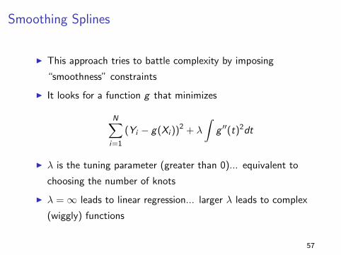
Smoothing Splines
I This approach tries to battle complexity by imposing
“smoothness” constraints
I It looks for a function g that minimizes
N∑i=1
(Yi − g(Xi ))2 + λ
∫g ′′(t)2dt
I λ is the tuning parameter (greater than 0)... equivalent to
choosing the number of knots
I λ =∞ leads to linear regression... larger λ leads to complex
(wiggly) functions
57
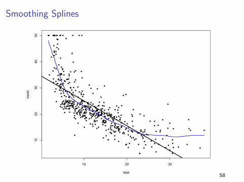
Smoothing Splines
10 20 30
1020
3040
50
lstat
medv
58
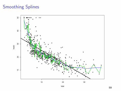
Smoothing Splines
10 20 30
1020
3040
50
lstat
medv
59
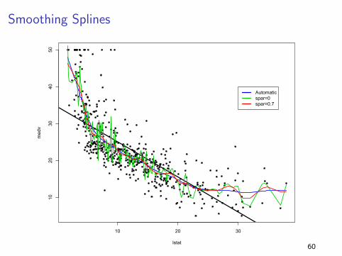
Smoothing Splines
10 20 30
1020
3040
50
lstat
medv
Automaticspar=0spar=0.7
60
Choosing the Model
How do we evaluate a forecasting model? Make predictions!
Basic Idea: We want to use the model to forecast outcomes for
observations we have not seen before.
I Use the data to create a prediction problem.
I See how our candidate models perform.
We’ll use most of the data for training the model,
and the left over part for validating the model.
61
Cross-Validation
In a cross-validation scheme, you fit a bunch of models to most of
the data (training sample) and choose the model
that performed the best on the rest (left-out sample).
I Use the model to obtain fitted Yj = x′jb values for all
of the NLO left-out data points.
I Calculate the Mean Square Error for these predictions.
MSE =1
NLO
NLO∑j=1
(Yj − Yj)2
62
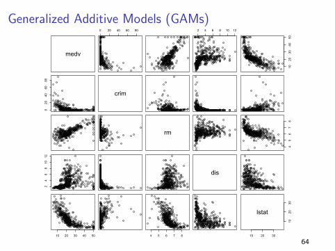
Generalized Additive Models (GAMs)
I We use “Gams” when we have more than one predictor
variable
I It tries to find a different non-linear function to connect each
X to Y ... and adds them all together (additive model).
Yi = β0 + f1(Xi1) + f2(Xi2) + · · ·+ fp(Xip) + ε
63
Generalized Additive Models (GAMs)
medv
0 20 40 60 80 2 4 6 8 10 12
1020
3040
50
020
4060
80
crim
rm
45
67
8
24
68
1012
dis
10 20 30 40 50 4 5 6 7 8 10 20 30
1020
30
lstat
64
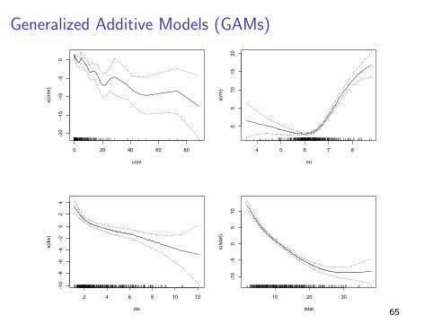
Generalized Additive Models (GAMs)
0 20 40 60 80
-20
-15
-10
-50
crim
s(crim)
4 5 6 7 8
05
1015
20
rm
s(rm)
2 4 6 8 10 12
-10
-8-6
-4-2
02
4
dis
s(dis)
10 20 30
-10
-50
510
lstat
s(lstat)
65
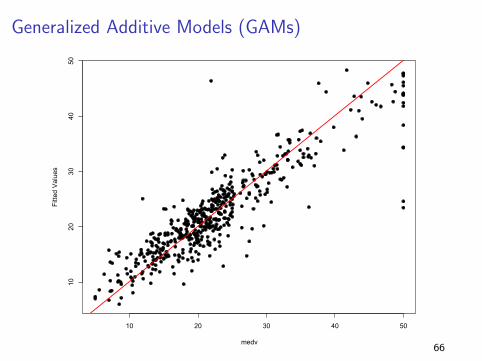
Generalized Additive Models (GAMs)
10 20 30 40 50
1020
3040
50
medv
Fitte
d V
alue
s
66
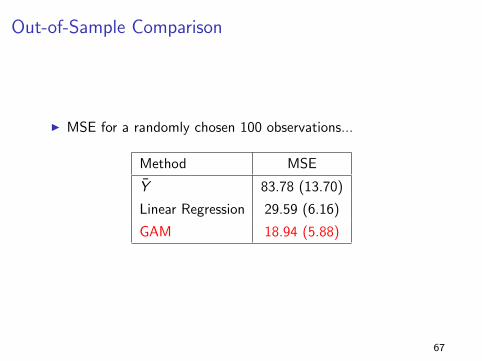
Out-of-Sample Comparison
I MSE for a randomly chosen 100 observations...
Method MSE
Y 83.78 (13.70)
Linear Regression 29.59 (6.16)
GAM 18.94 (5.88)
67
Model Building Process
When building a regression model remember that simplicity is your
friend... smaller models are easier to interpret and have fewer
unknown parameters to be estimated.
Keep in mind that every additional parameter represents a cost!!
The first step of every model building exercise is the selection of
the the universe of variables to be potentially used. This task is
entirely solved through you experience and context specific
knowledge...
I Think carefully about the problem
I Consult subject matter research and experts
I Avoid the mistake of selecting too many variables68
Model Building Process
With a universe of variables in hand, the goal now is to select the
model. Why not include all the variables in?
Big models tend to over-fit and find features that are specific to
the data in hand... ie, not generalizable relationships.
The results are bad predictions and bad science!
In addition, bigger models have more parameters and potentially
more uncertainty about everything we are trying to learn... (check
the beer and weight example!)
We need a strategy to build a model in ways that accounts for the
trade-off between fitting the data and the uncertainty associated
with the model 69
Out-of-Sample Prediction
One idea is to focus on the model’s ability to predict... How do we
evaluate a forecasting model? Make predictions!
Basic Idea: We want to use the model to forecast outcomes for
observations we have not seen before.
I Use the data to create a prediction problem.
I See how our candidate models perform.
We’ll use most of the data for training the model,
and the left over part for validating the model.
70
Out-of-Sample Prediction
In a cross-validation scheme, you fit a bunch of models to most of
the data (training sample) and choose the model
that performed the best on the rest (left-out sample).
I Fit the model on the training data
I Use the model to predict Yj values for all of the NLO left-out
data points
I Calculate the Mean Square Error for these predictions
MSE =1
NLO
NLO∑j=1
(Yj − Yj)2
71
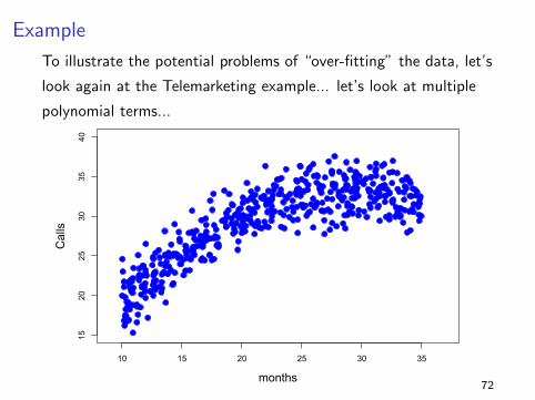
Example
To illustrate the potential problems of “over-fitting” the data, let’s
look again at the Telemarketing example... let’s look at multiple
polynomial terms...
10 15 20 25 30 35
1520
2530
3540
months
Calls
72
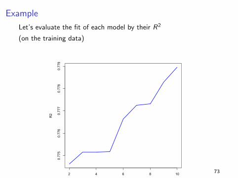
Example
Let’s evaluate the fit of each model by their R2
(on the training data)
2 4 6 8 10
0.775
0.776
0.777
0.778
0.779
Polynomial Order
R2
73
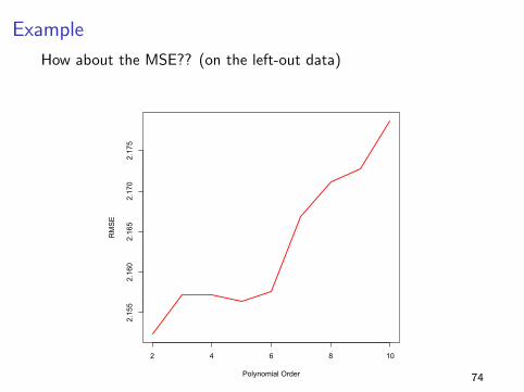
Example
How about the MSE?? (on the left-out data)
2 4 6 8 10
2.155
2.160
2.165
2.170
2.175
Polynomial Order
RMSE
74
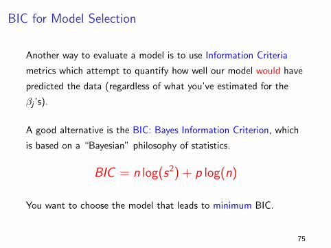
BIC for Model Selection
Another way to evaluate a model is to use Information Criteria
metrics which attempt to quantify how well our model would have
predicted the data (regardless of what you’ve estimated for the
βj ’s).
A good alternative is the BIC: Bayes Information Criterion, which
is based on a “Bayesian” philosophy of statistics.
BIC = n log(s2) + p log(n)
You want to choose the model that leads to minimum BIC.
75
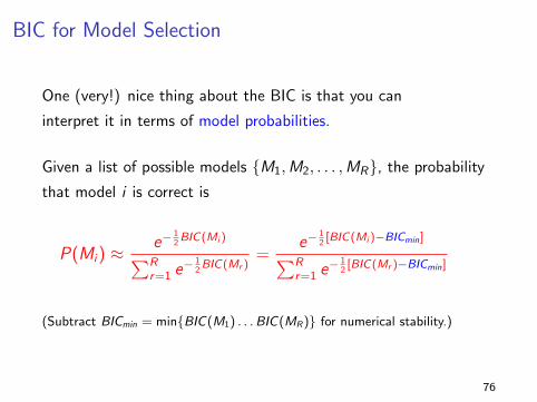
BIC for Model Selection
One (very!) nice thing about the BIC is that you can
interpret it in terms of model probabilities.
Given a list of possible models {M1,M2, . . . ,MR}, the probability
that model i is correct is
P(Mi) ≈e−
12BIC(Mi )∑R
r=1 e−12BIC(Mr )
=e−
12[BIC(Mi )−BICmin]∑R
r=1 e−12[BIC(Mr )−BICmin]
(Subtract BICmin = min{BIC(M1) . . .BIC(MR)} for numerical stability.)
76
BIC for Model Selection
Thus BIC is an alternative to testing for comparing models.
I It is easy to calculate.
I You are able to evaluate model probabilities.
I There are no “multiple testing” type worries.
I It generally leads to more simple models than F -tests.
As with testing, you need to narrow down your options before
comparing models. What if there are too many possibilities?
77
Stepwise Regression
One computational approach to build a regression model
step-by-step is “stepwise regression” There are 3 options:
I Forward: adds one variable at the time until no remaining
variable makes a significant contribution (or meet a certain
criteria... could be out of sample prediction)
I Backwards: starts will all possible variables and removes one
at the time until further deletions would do more harm them
good
I Stepwise: just like the forward procedure but allows for
deletions at each step
78
LASSO
The LASSO is a shrinkage method that performs automatic
selection. Yet another alternative... has similar properties as
stepwise regression but it is more automatic... R does it for you!
The LASSO solves the following problem:
arg minβ
{N∑
i=1
(Yi − X ′i β
)2+ λ|β|
}
I Coefficients can be set exactly to zero (automatic model
selection)
I Very efficient computational method
I λ is often chosen via CV
79
One informal but very useful idea to put it all together...
I like to build models from the bottom, up...
I Set aside a set of points to be your validating set (if dataset
large enought)I Working on the training data, add one variable at the time
deciding which one to add based on some criteria:
1. larger increases in R2 while significant
2. larger reduction in MSE while significant
3. BIC, etc...
I at every step, carefully analyze the output and
check the residuals!
I Stop when no additional variable produces a “significant”
improvement
I Always make sure you understand what the model is doing in
the specific context of your problem80