Additive Mixed Models for Correlated Functional Data

Additive Mixed Models forCorrelated Functional Data

Fabian Scheipl

Institut fur StatistikLudwig-Maximilians-Universitat Munchen

SuSTaIn Workshop”High Dimensional and Dependent Functional Data”

September 10, 2012

Joint work with C. Crainiceanu, S. Greven, A. Ivanescu, P. Reiss, A.-M. Staicu

Scheipl, Staicu, Greven (2012) Function-on-Function AMMs 1 / 25

Model

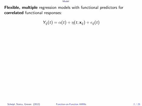
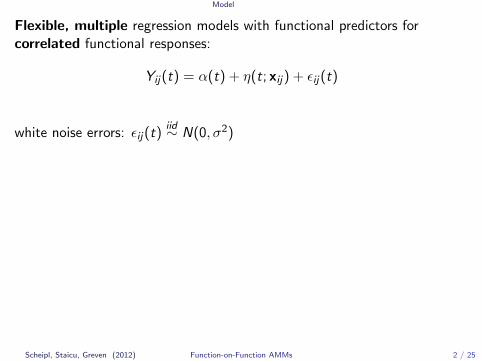
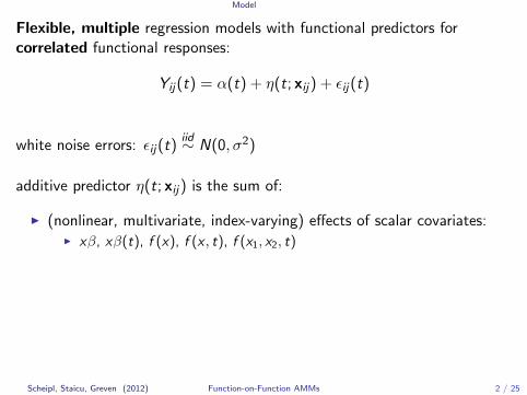
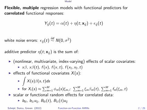
Flexible, multiple regression models with functional predictors forcorrelated functional responses:

Yij(t) = α(t) + η(t; xij) + εij(t)

white noise errors: εij(t)iid∼ N(0, σ2)

additive predictor η(t; xij) is the sum of:

I (nonlinear, multivariate, index-varying) effects of scalar covariates:I xβ, xβ(t), f (x), f (x , t), f (x1, x2, t)

I effects of functional covariates X (s):

I

∫X (s)β(s, t)ds

I for Xi (s) ≈∑M

m=1 φm(s)ξm,i :∑M

m=1 ξmβm(t),∑M

m=1 fm(ξm, t)

I scalar or functional random effects for correlated data:I b0i , b1iuij , B0i (t), B1i (t)uij


Model

This is just a kind of varying coefficient model...

... effects vary over index of response:

I write as model for concatenated function values vec

(Yn×T

)I reformat covariate data accordingly & add index t as covariate

⇒ can be fitted like standard AMM for scalar responses usingpenalized splines

I effects vary smoothly over t ⇒ smoothness of E (Y (t))

I sparse/irregular Y (t) possible


Model

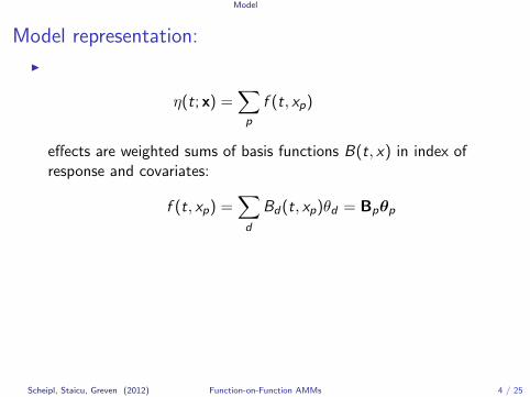
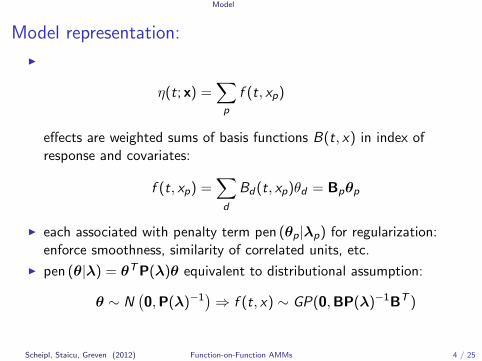
Model representation:

I

η(t; x) =∑p

f (t, xp)

effects are weighted sums of basis functions B(t, x) in index ofresponse and covariates:

f (t, xp) =∑d

Bd(t, xp)θd = Bpθp

I each associated with penalty term pen (θp|λp) for regularization:enforce smoothness, similarity of correlated units, etc.

I pen (θ|λ) = θTP(λ)θ equivalent to distributional assumption:

θ ∼ N(0,P(λ)−1

)⇒ f (t, x) ∼ GP(0,BP(λ)−1BT )


Model

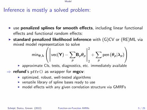
Inference is mostly a solved problem:

I use penalized splines for smooth effects, including linear functionaleffects and functional random effects:

I standard penalized likelihood inference with (G)CV or (RE)ML viamixed model representation to solve

minθ,λ

∥∥∥∥∥vec(Y)−∑p

Bpθp

∥∥∥∥∥2

2

+∑p

pen (θp|λp)

I approximate CIs, tests, diagnostics, etc. immediately available

⇒ refund’s pffr() as wrapper for mgcv:I optimized, robust, well-tested algorithmsI versatile library of spline bases ready to useI model effects with any given correlation structure via GMRFs


Model

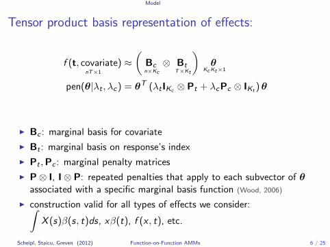
Tensor product basis representation of effects:

f (t, covariate)nT×1

≈(

Bcn×Kc

⊗ BtT×Kt

)θ

KcKt×1

pen(θ|λt , λc) = θT (λtIKc ⊗ Pt + λcPc ⊗ IKt )θ

I Bc : marginal basis for covariate

I Bt : marginal basis on response’s index

I Pt ,Pc : marginal penalty matrices

I P⊗ I, I⊗ P: repeated penalties that apply to each subvector of θassociated with a specific marginal basis function (Wood, 2006)

I construction valid for all types of effects we consider:∫X (s)β(s, t)ds, xβ(t), f (x , t), etc.


Model

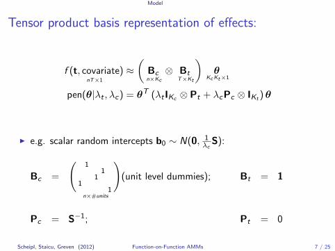
Tensor product basis representation of effects:

f (t, covariate)nT×1

≈(

Bcn×Kc

⊗ BtT×Kt

)θ

KcKt×1

pen(θ|λt , λc) = θT (λtIKc ⊗ Pt + λcPc ⊗ IKt )θ

I e.g. scalar random intercepts b0 ∼ N(0, 1λc

S):

Bc =

(1

11

11

)n×#units

(unit level dummies); Bt = 1

Pc = S−1; Pt = 0


Functional Random Effects

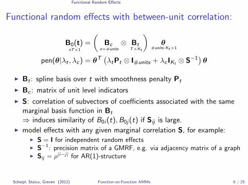
Functional random effects with between-unit correlation:

B0(t)nT×1

=

(Bc

n×#units

⊗ BtT×Kt

)θ

#units·Kt×1

pen(θ|λt , λc) = θT(λtPt ⊗ I#units + λc IKt ⊗ S−1

)θ

I Bt : spline basis over t with smoothness penalty Pt

I Bc : matrix of unit level indicators

I S: correlation of subvectors of coefficients associated with the samemarginal basis function in Bt

⇒ induces similarity of B0i (t),B0j(t) if Sij is large.I model effects with any given marginal correlation S, for example:

I S = I for independent random effectsI S−1: precision matrix of a GMRF, e.g. via adjacency matrix of a graphI Sij = ρ|i−j| for AR(1)-structure


Functional Random Effects

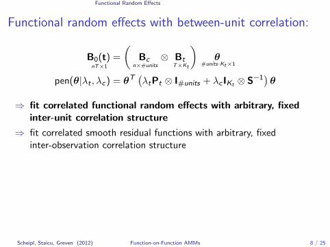
Functional random effects with between-unit correlation:

B0(t)nT×1

=

(Bc

n×#units

⊗ BtT×Kt

)θ

#units·Kt×1

pen(θ|λt , λc) = θT(λtPt ⊗ I#units + λc IKt ⊗ S−1

)θ

⇒ fit correlated functional random effects with arbitrary, fixedinter-unit correlation structure

⇒ fit correlated smooth residual functions with arbitrary, fixedinter-observation correlation structure


Empirical Evaluation

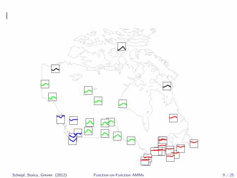
Example: Canadian Weather Data



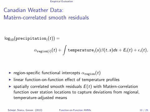
Canadian Weather Data:Matern-correlated smooth residuals

log10(precipitationi (t)) =

αregion(i)(t) +

∫temperaturei (s)β(t, s)ds + Ei (t) + εi (t),

I region-specific functional intercepts αregion(t)

I linear function-on-function effect of temperature profiles

I spatially correlated smooth residuals E (t) with Matern-correlationfunction over station locations to capture deviations from regional,temperature-adjusted means



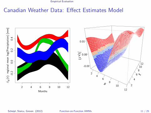
Canadian Weather Data: Effect Estimates Model

2 4 6 8 10 12

-0.2

0.0

0.2

0.4

Months

αgi(t):

region

almeanlog(Precipitation)[m

m]

s

24

68

10

12

t

2

4

6

81012

.β(s,t)

-0.01

0.00

0.01



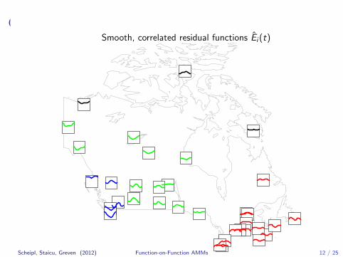
Canadian Weather Data: Effect EstimatesSmooth, correlated residual functions Ei (t)



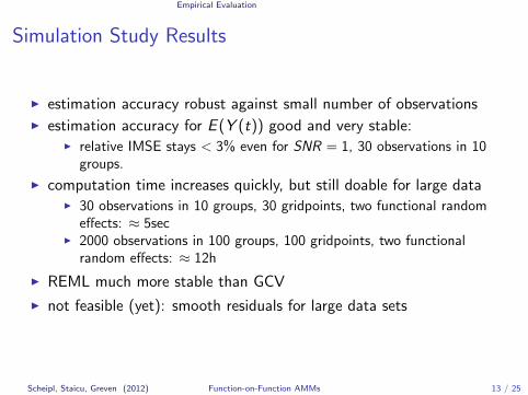
Simulation Study Results

I estimation accuracy robust against small number of observationsI estimation accuracy for E (Y (t)) good and very stable:

I relative IMSE stays < 3% even for SNR = 1, 30 observations in 10groups.

I computation time increases quickly, but still doable for large dataI 30 observations in 10 groups, 30 gridpoints, two functional random

effects: ≈ 5secI 2000 observations in 100 groups, 100 gridpoints, two functional

random effects: ≈ 12h

I REML much more stable than GCV

I not feasible (yet): smooth residuals for large data sets


.

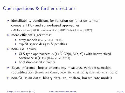
Open questions & further directions:

I identifiability conditions for function-on-function terms:compare FPC- and spline-based approaches(Muller and Yao, 2008; Ivanescu et al., 2012; Scheipl et al., 2012)

I more efficient algorithms:I array models (Currie et al., 2006)

I exploit sparse designs & penalties

I non-i.i.d. errors:I GLS-type approaches: εij(t)

iid∼ GP(0,K (t, t ′)) with known/fixedcovariance K (t, t ′) (Reiss et al., 2010)

I bootstrap-based inference

I Bayes inference: better uncertainty measures, variable selection,robustification (Morris and Carroll, 2006; Zhu et al., 2011; Goldsmith et al., 2011)

I non-Gaussian data: binary data, count data, hazard rate models


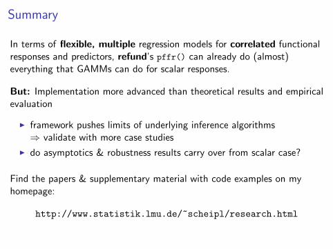
Summary

In terms of flexible, multiple regression models for correlated functionalresponses and predictors, refund’s pffr() can already do (almost)everything that GAMMs can do for scalar responses.

But: Implementation more advanced than theoretical results and empiricalevaluation

I framework pushes limits of underlying inference algorithms⇒ validate with more case studies

I do asymptotics & robustness results carry over from scalar case?

Find the papers & supplementary material with code examples on myhomepage:

http://www.statistik.lmu.de/~scheipl/research.html

http://www.statistik.lmu.de/~scheipl/research.html

.

References

H. Cardot, F. Ferraty, and P. Sarda. Functional linear model. Statistics and Probability Letters, 45:11–22, 1999.

I.D. Currie, M. Durban, and P.H.C. Eilers. Generalized linear array models with applications to multidimensional smoothing.Journal of the Royal Statistical Society: Series B (Statistical Methodology), 68(2):259–280, 2006.

J. Goldsmith, M.P. Wand, and C. Crainiceanu. Functional regression via variational bayes. Electronic Journal of Statistics, 5:572, 2011.

G. He, H.G. Muller, and J.L. Wang. Extending correlation and regression from multivariate to functional data. In M.L. Puri,editor, Asymptotics in Statistics and Probability, pages 301 – 315. VSP International Science Publishers, 2003.

A.E. Ivanescu, A.-M. Staicu, S. Greven, F. Scheipl, and C.M. Crainiceanu. Penalized function-on-function regression. 2012.URL http://biostats.bepress.com/jhubiostat/paper240/. submitted.

J.S. Morris and R.J. Carroll. Wavelet-based functional mixed models. Journal of the Royal Statistical Society: Series B(Statistical Methodology), 68(2):179–199, 2006.

H.G. Muller and F. Yao. Functional additive models. Journal of the American Statistical Association, 103(484):1534–1544, 2008.

P. Reiss, L. Huang, and M. Mennes. Fast function-on-scalar regression with penalized basis expansions. The InternationalJournal of Biostatistics, 6(1):28, 2010.

F. Scheipl and S. Greven. Identifiability in penalized function-on-function regression models. Technical Report 125, LMUMunchen, 2012. URL http://epub.ub.uni-muenchen.de/13060/.

F. Scheipl, A.-M. Staicu, and S. Greven. Additive Mixed Models for Correlated Functional Data. 2012. URLhttp://arxiv.org/abs/1207.5947. submitted.

S.N. Wood. Generalized Additive Models: An Introduction with R. Chapman & Hall/CRC, 2006.

H. Zhu, P.J. Brown, and J.S. Morris. Robust, adaptive functional regression in functional mixed model framework. Journal ofthe American Statistical Association, 106(495):1167–1179, 2011.


http://biostats.bepress.com/jhubiostat/paper240/

http://epub.ub.uni-muenchen.de/13060/

http://arxiv.org/abs/1207.5947

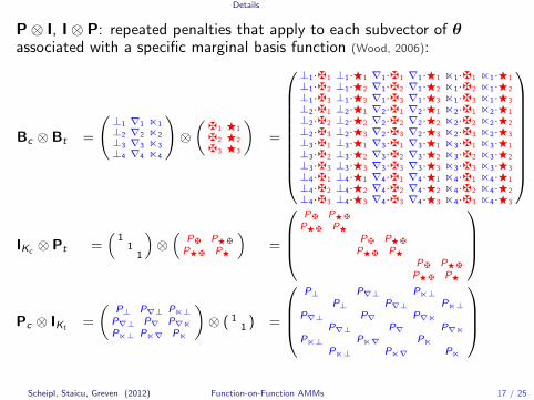
Details

P⊗ I, I⊗ P: repeated penalties that apply to each subvector of θassociated with a specific marginal basis function (Wood, 2006):

Bc ⊗ Bt =

(⊥1 ∇1 n1

⊥2 ∇2 n2

⊥3 ∇3 n3

⊥4 ∇4 n4

)⊗(

z1 F1

z2 F2

z3 F3

)=

⊥1·z1 ⊥1·F1 ∇1·z1 ∇1·F1 n1·z1 n1·F1

⊥1·z2 ⊥1·F2 ∇1·z2 ∇1·F2 n1·z2 n1·F2

⊥1·z3 ⊥1·F3 ∇1·z3 ∇1·F3 n1·z3 n1·F3

⊥2·z1 ⊥2·F1 ∇2·z1 ∇2·F1 n2·z1 n2·F1

⊥2·z2 ⊥2·F2 ∇2·z2 ∇2·F2 n2·z2 n2·F2

⊥2·z3 ⊥2·F3 ∇2·z3 ∇2·F3 n2·z3 n2·F3

⊥3·z1 ⊥3·F1 ∇3·z1 ∇3·F1 n3·z1 n3·F1

⊥3·z2 ⊥3·F2 ∇3·z2 ∇3·F2 n3·z2 n3·F2

⊥3·z3 ⊥3·F3 ∇3·z3 ∇3·F3 n3·z3 n3·F3

⊥4·z1 ⊥4·F1 ∇4·z1 ∇4·F1 n4·z1 n4·F1

⊥4·z2 ⊥4·F2 ∇4·z2 ∇4·F2 n4·z2 n4·F2

⊥4·z3 ⊥4·F3 ∇4·z3 ∇4·F3 n4·z3 n4·F3

IKc ⊗ Pt =(

11

1

)⊗(

Pz PFz

PFz PF

)=

Pz PFz

PFz PF

Pz PFz

PFz PF

Pz PFz

PFz PF

Pc ⊗ IKt =

(P⊥ P∇⊥ Pn⊥P∇⊥ P∇ P∇nPn⊥ Pn∇ Pn

)⊗ ( 1

1 ) =

P⊥ P∇⊥ Pn⊥

P⊥ P∇⊥ Pn⊥P∇⊥ P∇ P∇n

P∇⊥ P∇ P∇nPn⊥ Pn∇ Pn

Pn⊥ Pn∇ Pn


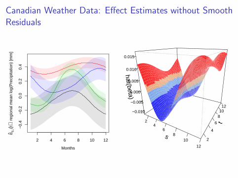
Canadian Weather Data: Effect Estimates without SmoothResiduals

2 4 6 8 10 12

−0.

4−

0.2

0.0

0.2

0.4

Months

α g_i(t)

: re

gion

al m

ean

log(

Pre

cipi

tatio

n) [m

m]

s

24

68

10

12

t

2

4

6

81012

hat(beta)−0.010

−0.005

0.000

0.005

0.010

0.015

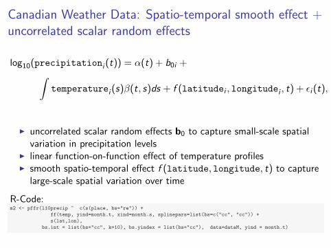
Canadian Weather Data: Spatio-temporal smooth effect +uncorrelated scalar random effects

log10(precipitationi (t)) = α(t) + b0i +∫temperaturei (s)β(t, s)ds + f (latitudei , longitudei , t) + εi (t),

I uncorrelated scalar random effects b0 to capture small-scale spatialvariation in precipitation levels

I linear function-on-function effect of temperature profilesI smooth spatio-temporal effect f (latitude, longitude, t) to capture

large-scale spatial variation over time

R-Code:m2 <- pffr(l10precip ~ c(s(place, bs="re")) +

ff(temp, yind=month.t, xind=month.s, splinepars=list(bs=c("cc", "cc")) +

s(lat,lon),

bs.int = list(bs="cc", k=10), bs.yindex = list(bs="cc"), data=dataM, yind = month.t)

Canadian Weather Data: Effect Estimates

Issues

Flexibility - Overfitting - Concurvity

very flexible models → danger of overfitting→ overparameterization? identifiability?

functional concurvity → useful analogies to scalar concurvity?

no good metrics/diagnostics for these issues yet


Issues

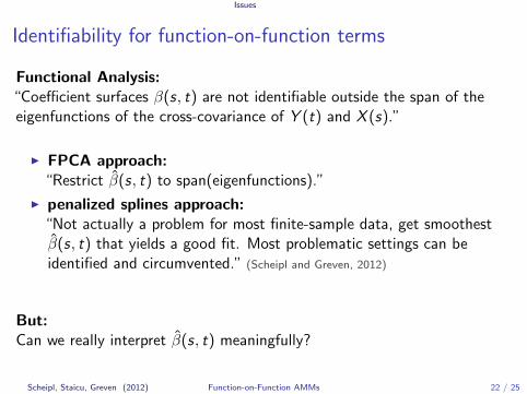
Identifiability for function-on-function terms

Functional Analysis:“Coefficient surfaces β(s, t) are not identifiable outside the span of theeigenfunctions of the cross-covariance of Y (t) and X (s).”

I FPCA approach:“Restrict β(s, t) to span(eigenfunctions).”

I penalized splines approach:“Not actually a problem for most finite-sample data, get smoothestβ(s, t) that yields a good fit. Most problematic settings can beidentified and circumvented.” (Scheipl and Greven, 2012)

But:Can we really interpret β(s, t) meaningfully?


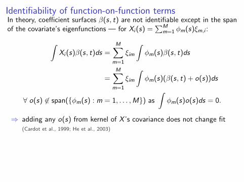
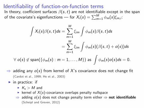
Identifiability of function-on-function termsIn theory, coefficient surfaces β(s, t) are not identifiable except in the spanof the covariate’s eigenfunctions — for Xi (s) =

∑Mm=1 φm(s)ξm,i :∫

Xi (s)β(s, t)ds =M∑

m=1

ξim

∫φm(s)β(s, t)ds

=M∑

m=1

ξim

∫φm(s)(β(s, t) + o(s))ds

∀ o(s) 6∈ span({φm(s) : m = 1, . . . ,M}) as

∫φm(s)o(s)ds = 0.

⇒ adding any o(s) from kernel of X ’s covariance does not change fit(Cardot et al., 1999; He et al., 2003)

I in practice: ifI Ks > M andI kernel of X (s)-covariance overlaps penalty nullspace⇒ adding o(s) does not change penalty term either ⇒ not identifiable

(Scheipl and Greven, 2012)

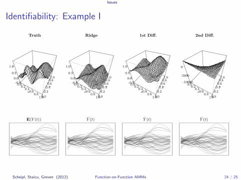
Issues

Identifiability: Example I

s

0.00.2

0.40.6

0.81.0

t

0.0

0.20.40.60.81.0

-0.50.0

0.5

1.0

Truth

s

0.00.2

0.40.6

0.81.0

t

0.0

0.20.40.60.81.0

-0.50.0

0.5

1.0

Ridge

s

0.00.2

0.40.6

0.81.0

t

0.0

0.20.40.60.81.0

-0.50.0

0.5

1.0

1st Diff.

s

0.00.2

0.40.6

0.81.0

t

0.0

0.20.40.60.81.0

-10000

-5000

0

2nd Diff.

E(Y (t)) Y (t) Y (t) Y (t)


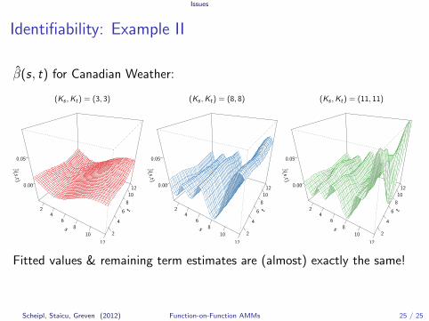
Issues

Identifiability: Example II

β(s, t) for Canadian Weather:

s

24

68

10

12

t

2

4

6

8

10

12

.β(s,t)

0.00

0.05

(Ks ,Kt) = (3, 3)

s

24

68

10

12

t

2

4

6

8

10

12

.β(s,t)

0.00

0.05

(Ks ,Kt) = (8, 8)

s

24

68

10

12

t

2

4

6

8

10

12

.β(s,t)

0.00

0.05

(Ks ,Kt) = (11, 11)

Fitted values & remaining term estimates are (almost) exactly the same!


Additive Mixed Models for Correlated Functional Data

Documents

Transcript of Additive Mixed Models for Correlated Functional Data