Acceleration with a Ball Optimization Oracle

Yair Carmon∗ Arun Jambulapati∗ Qijia Jiang∗ Yujia Jin∗ Yin Tat Lee†Aaron Sidford∗ Kevin Tian∗

AbstractConsider an oracle which takes a point x and returns the minimizer of a convex function f in

an `2 ball of radius r around x. It is straightforward to show that roughly r−1 log 1ε calls to the

oracle suffice to find an ε-approximate minimizer of f in an `2 unit ball. Perhaps surprisingly, thisis not optimal: we design an accelerated algorithm which attains an ε-approximate minimizerwith roughly r−2/3 log 1

ε oracle queries, and give a matching lower bound. Further, we implementball optimization oracles for functions with locally stable Hessians using a variant of Newton’smethod. The resulting algorithm applies to a number of problems of practical and theoreticalimport, improving upon previous results for logistic and `∞ regression and achieving guaranteescomparable to the state-of-the-art for `p regression.

1 IntroductionWe study unconstrained minimization of a smooth convex objective f : Rd → R, which we accessthrough a ball optimization oracle Oball, that when queried at any point x, returns the minimizer1

of f restricted a ball of radius r around x, i.e.,

Oball(x) = arg minx′ s.t. ‖x′−x‖≤r

f(x′).

Such oracles underlie trust region methods [12] and, as we demonstrate via applications, encap-sulate problems with local stability. Iterating xk+1 ← Oball(xk) minimizes f in O(R/r) iterations(see Appendix A), where R is the initial distance to the minimizer, x∗, and O(·) hides polyloga-rithmic factors in problem parameters, including the desired accuracy.

Given the fundamental geometric nature of the ball optimization abstraction, the central ques-tion motivating our work is whether it is possible to improve upon this O(R/r) query complexity.It is natural to conjecture that the answer is negative: we require R/r oracle calls to observe theentire line from x0 to the optimum, and therefore finding a solution using less queries would re-quire jumping into completely unobserved regions. Nevertheless, we prove that the optimal querycomplexity scales as (R/r)2/3. This result has positive implications for the complexity for severalkey regression tasks, for which we can efficiently implement the ball optimization oracles.

1.1 Our contributions

Here we overview the main contributions of our paper: accelerating ball optimization oracles (witha matching lower bound), implementing them under Hessian stability, and applying the resultingtechniques to regression problems.∗Stanford University, yairc,jmblpati,qjiang2,yujiajin,sidford,kjtian@stanford.edu.†University of Washington, yintat@uw.edu.1In the introduction we discuss exact oracles for simplicity, but our results account for inexactness.

1

arX

iv:2

003.

0807

8v1

[m

ath.

OC

] 1

8 M

ar 2

020

Monteiro-Svaiter (MS) oracles via ball optimization. Our starting point is an accelerationframework due to Monteiro and Svaiter [20]. It relies on access to an oracle that when queried withx, v ∈ Rd and A > 0, returns points x+, y ∈ Rd and λ > 0 such that

y = A

A+ aλx+ aλ

A+ aλv, and (1)

x+ ≈ arg minx′∈Rd

f(x′) + 1

2λ‖x′ − y‖2

, (2)

where aλ = 12(λ +

√λ2 + 4Aλ). Basic calculus shows that for any z, the radius-r oracle response

Oball(z) solves the proximal point problem (2) for y = z and some λ = λr(z) ≥ 0 which depends onr and z. Therefore, to implement the MS oracle with a ball optimization oracle, we need to find λthat solves the implicit equation λ = λr(y(λ)), with y(λ) as in (1). We accomplish an approximateversion of this via binary search over λ, resulting in an accelerated scheme that makes O(1) queriesto Oball(·) per iteration (each iteration also requires a gradient evaluation).

The main challenge lies in proving that our MS oracle implementation guarantees rapid con-vergence. We do so by a careful analysis which relates convergence to the distance between thepoints y and x+ that the MS oracle outputs. Specifically, letting yk, xk+1 be the sequence ofthese points, we prove that

f(xK)− f(x∗)f(x0)− f(x∗) ≤ exp

−Ω(K) min

k<K

‖xk+1 − yk‖2/3

R2/3

.

Since Oball guarantees ‖xk+1 − yk‖ = r for all k except possibly the last (if the final ball containsx∗), our result follows.

Matching lower bound. We give a distribution over functions with domain of size R for whichany algorithm interacting with a ball optimization oracle of radius r requires Ω((R/r)2/3) queriesto find an approximate solution with O(r1/3) additive error. Our lower bound in fact holds for aneven more powerful r-local oracle, which reveals all values of f in a ball of radius r around the querypoint. We prove our lower bounds using well-established techniques and Nemirovski’s function, acanonical hard instance in convex optimization [21, 25, 10, 14, 8]. Here, our primary contribution isto show that appropriately scaling this construction makes it hard even against r-local oracles witha fixed radius r, as opposed to the more standard notion of local oracles that reveal the instanceonly in an arbitrarily small neighborhood around the query.

Implementation of a ball optimization oracle. Trust region methods [12] solve a sequenceof subproblems of the form

minimizeδ∈Rd s.t. ‖δ‖≤r

δ>g + 1

2δ>Hδ

.

When g = ∇f(x) and H = ∇2f(x), the trust region subproblem minimizes a second-order Taylorexpansion of f around x, implementing an approximate ball optimization oracle. We show how toimplement a ball optimization oracle for f to high accuracy for functions satisfying a local Hessianstability property. Specifically, we use a notion of Hessian stability similar to that of Karimireddyet al. [18], requiring 1

c∇2f(x) ∇2f(y) c∇2f(x) for every y in a ball of radius r around x for

some c > 1. We analyze Nesterov’s accelerated gradient method in a Euclidean norm weighted bythe Hessian at x, which we can also view as accelerated Newton steps, and show that it implementsthe oracle in O(c) linear system solutions. Here acceleration improves upon the c2 dependence ofmore naive methods. This improvement is not necessary for our applications where we take c tobe a constant, but we include it for completeness.

2

Applications. We apply our implementation and acceleration of ball optimization oracles toproblems of the form f(Ax− b) for data matrix A ∈ Rn×d. For logistic regression, where

f(z) =∑i∈[n]

log(1 + e−zi),

the Hessian stability property [4] implies that our algorithm solves the problem with O(‖x0 −x∗‖2/3A>A) linear system solves of the form A>DAx = z for diagonal matrix D. This improves uponthe previous best linearly-convergent condition-free algorithm due to Karimireddy et al. [18], whichrequires O(‖x0 − x∗‖A>A) system solves. Our improvement is precisely the power 2/3 factor thatcomes from acceleration using the ball optimization oracle.

For `∞ regression, we take f to be the log-sum-exp (softmax) function and establish that it toohas a stable Hessian. By appropriately scaling softmax to approximate `∞ to ε additive error andtaking r = ε, we obtain an algorithm that solves `∞ to additive error ε in O(‖x0 − x∗‖2/3A>Aε

−2/3)linear system solves of the same form as above. This improves upon the algorithm of Bullins andPeng [9] which requires O(‖x0 − x∗‖4/5A>Aε

−4/5) linear system solves.Finally, we leverage our implementation of a ball optimization oracle to obtain high accuracy

solutions to `p norm regression, where f(z) =∑i∈[n] |zi|p. Here, we use our accelerated ball-

constrained Newton algorithm to minimize a sequence of proximal problems with a geometricallyshrinking quadratic regularization term. The result is an algorithm that solves O(poly(p)n1/3)linear systems. For p = ω(1), this matches the state-of-the-art n dependence [1] but obtains aworse dependence on p. Nevertheless, our approach seems simpler than prior work and leaves roomfor further refinements which we believe will result in stronger guarantees.

1.2 Related work

Our developments are rooted in three lines of work, which we now briefly survey.

Monteiro-Svaiter framework instantiations. Monteiro and Svaiter [20] propose a new ac-celeration framework, which they specialize to recover the classic fast gradient method [22] andobtain an optimal accelerated second-order method for convex problems with Lipschitz Hessian.Subsequent work [15] extends this to functions with pth-order Lipschitz derivatives and a pth-orderoracle. Generalizing further, Bubeck et al. [8] implement the MS oracle via a “Φ prox” oracle thatgiven query x returns roughly arg minx′f(x) + Φ(‖x′−x‖), for continuously differentiable Φ, andprove an error bound scaling with the iterate number k as φ(R/k3/2)R2/k2, where φ(t) = Φ′(t)/t.Using poly(d) parallel queries to a subgradient oracle for non-smooth f , they show how to imple-ment the Φ prox oracle for Φ(t) ∝ (t/r)p with arbitrarily large p, where r = ε/

√d. Our notion of

a ball optimization corresponds to taking p =∞, i.e., letting Φ be the indicator of [0, r]. However,since such Φ is not continuous, our result does not follow directly from [8]. Thus, our approachclarifies the limiting behavior of MS acceleration of infinitely smooth functions.

Trust region methods. The idea of approximately minimizing the objective in a “trust region”around the current iterate plays a central role in nonlinear optimization and machine learning [see,e.g., 12, 19, 23]. Typically, the approximation takes the form of a second-order Taylor expansion,where regularity of the Hessian is key for guaranteeing the approximation quality. Of particularrelevance to us is the work of Karimireddy et al. [18], which define a notion of Hessian stabilityunder which a trust region method converges linearly with only logarithmic dependence on problemconditioning. We observe that this stability condition in fact renders the second-order trust region

3

approximation highly effective, so that a few iterations suffice in order to implement an “ideal” balloptimization oracle, thus enabling accelerated condition-free convergence.

Efficient `p regression algorithms. There has been rapid recent progress in linearly convergentalgorithms for minimizing the p-norm of the regression residual Ax−b or alternatively for finding aminimum p-norm x satisfying the linear constraints Ax = b. Bubeck et al. [7] give faster algorithmsfor all p ∈ (1, 2)∪ (2,∞), discovering and overcoming a limitation of classic interior point methods.Their algorithm is based on considering a “smoother” objective which behaves as a quadratic withina region, and as the original pth-order objective outside. Adil et al. [2] improve on this result withan algorithm with iteration complexity bounded by n1/3 (for regression in n constraints) for allp bounded away from 1 and ∞, improving upon the n1/2 limit behavior of Bubeck et al. [7].Adil and Sachdeva [1] provide an alternative method which achieves n1/3 iterations with a lineardependence on p, improving on the O(pO(p)) dependence found in Adil et al. [2]. For p = ∞,Bullins and Peng [9] develop a method based on fourth-order MS acceleration for ε-approximatelyminimizing the smooth softmax approximation to the `∞ objective, with iteration complexity ε−4/5.We believe that our approach brings us closer to a unified perspective on high-order smoothnessand acceleration for regression problems.

1.3 Paper organization

In Section 2, we implement the MS oracle using a ball optimization oracle and prove its O((R/r)2/3)convergence guarantee. In Section 3, we show how to use Hessian stability to efficiently implementa ball optimization oracle, and also show that quasi-self-concordance implies Hessian stability. InSection 4 we apply our developments to the aforementioned regression tasks. Finally, in Section 5we give a lower bound implying our oracle complexity is optimal (up to logarithmic terms).

Notation. Let M be a positive semidefinite matrix, and let M† be its pseudoinverse. We performour analysis in the Euclidean seminorm ‖x‖M

def=√x>Mx; we will choose a specific M when

discussing applications. We denote the ‖·‖M ball of radius r around x by

Br(x) def=x ∈ Rd | ‖x− x‖M ≤ r

.

We recall standard definitions of smoothness and strong-convexity in a quadratic norm: differen-tiable f : Rd → R is L-smooth in ‖·‖M if its gradient is L-Lipschitz in ‖·‖M, and twice-differentiablef is L-smooth and µ-strongly convex in ‖·‖M if µM ∇2f(x) LM for all x ∈ Rd.

2 Monteiro-Svaiter Acceleration with a Ball Optimization OracleIn this section, we give an accelerated algorithm for optimization with the following oracle.

Definition 1 (Ball optimization oracle). We call Oball a (δ, r)-ball optimization oracle for f :Rd → R if for any x ∈ Rd, it outputs y = Oball(x) ∈ Br(x) such that ‖y − xx,r‖M ≤ δ for somexx,r ∈ arg minx∈Br(x) f(x).

Our algorithm utilizes the acceleration framework of Monteiro and Svaiter [20] (see also [15, 8]).It relies on the following oracle.

4

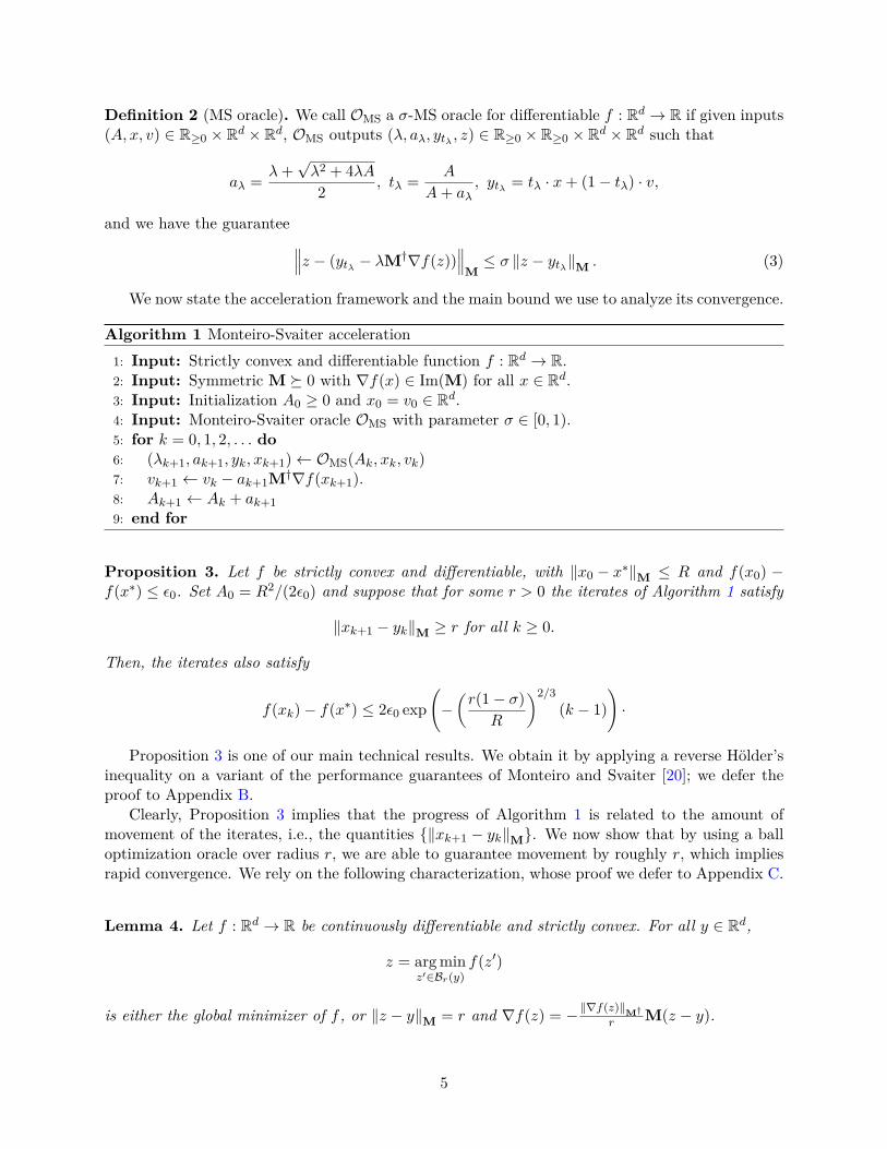
Definition 2 (MS oracle). We call OMS a σ-MS oracle for differentiable f : Rd → R if given inputs(A, x, v) ∈ R≥0 × Rd × Rd, OMS outputs (λ, aλ, ytλ , z) ∈ R≥0 × R≥0 × Rd × Rd such that

aλ = λ+√λ2 + 4λA2 , tλ = A

A+ aλ, ytλ = tλ · x+ (1− tλ) · v,

and we have the guarantee ∥∥∥z − (ytλ − λM†∇f(z))∥∥∥

M≤ σ ‖z − ytλ‖M . (3)

We now state the acceleration framework and the main bound we use to analyze its convergence.

Algorithm 1 Monteiro-Svaiter acceleration1: Input: Strictly convex and differentiable function f : Rd → R.2: Input: Symmetric M 0 with ∇f(x) ∈ Im(M) for all x ∈ Rd.3: Input: Initialization A0 ≥ 0 and x0 = v0 ∈ Rd.4: Input: Monteiro-Svaiter oracle OMS with parameter σ ∈ [0, 1).5: for k = 0, 1, 2, . . . do6: (λk+1, ak+1, yk, xk+1)← OMS(Ak, xk, vk)7: vk+1 ← vk − ak+1M†∇f(xk+1).8: Ak+1 ← Ak + ak+19: end for

Proposition 3. Let f be strictly convex and differentiable, with ‖x0 − x∗‖M ≤ R and f(x0) −f(x∗) ≤ ε0. Set A0 = R2/(2ε0) and suppose that for some r > 0 the iterates of Algorithm 1 satisfy

‖xk+1 − yk‖M ≥ r for all k ≥ 0.

Then, the iterates also satisfy

f(xk)− f(x∗) ≤ 2ε0 exp(−(r(1− σ)

R

)2/3(k − 1)

)·

Proposition 3 is one of our main technical results. We obtain it by applying a reverse Hölder’sinequality on a variant of the performance guarantees of Monteiro and Svaiter [20]; we defer theproof to Appendix B.

Clearly, Proposition 3 implies that the progress of Algorithm 1 is related to the amount ofmovement of the iterates, i.e., the quantities ‖xk+1 − yk‖M. We now show that by using a balloptimization oracle over radius r, we are able to guarantee movement by roughly r, which impliesrapid convergence. We rely on the following characterization, whose proof we defer to Appendix C.

Lemma 4. Let f : Rd → R be continuously differentiable and strictly convex. For all y ∈ Rd,

z = arg minz′∈Br(y)

f(z′)

is either the global minimizer of f , or ‖z − y‖M = r and ∇f(z) = −‖∇f(z)‖M†r M(z − y).

5

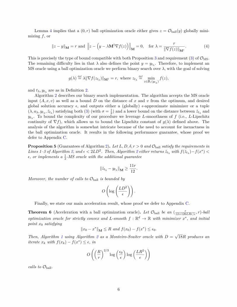
Lemma 4 implies that a (0, r) ball optimization oracle either gives z = Oball(y) globally mini-mizing f , or

‖z − y‖M = r and∥∥∥z − (y − λM†∇f(z)

)∥∥∥M

= 0, for λ = r

‖∇f(z)‖M†. (4)

This is precisely the type of bound compatible with both Proposition 3 and requirement (3) of OMS.The remaining difficulty lies in that λ also defines the point y = ytλ . Therefore, to implement anMS oracle using a ball optimization oracle we perform binary search over λ, with the goal of solving

g(λ) def= λ‖∇f(ztλ)‖M† = r, where ztλdef= min

z∈Br(ytλ )f(z),

and tλ, ytλ are as in Definition 2.Algorithm 2 describes our binary search implementation. The algorithm accepts the MS oracle

input (A, x, v) as well as a bound D on the distance of x and v from the optimum, and desiredglobal solution accuracy ε, and outputs either a (globally) ε-approximate minimizer or a tuple(λ, aλ, ytλ , ztλ) satisfying both (3) (with σ = 1

2) and a lower bound on the distance between ztλ andytλ . To bound the complexity of our procedure we leverage L-smoothness of f (i.e., L-Lipschitzcontinuity of ∇f), which allows us to bound the Lipschitz constant of g(λ) defined above. Theanalysis of the algorithm is somewhat intricate because of the need to account for inexactness inthe ball optimization oracle. It results in the following performance guarantee, whose proof wedefer to Appendix C.

Proposition 5 (Guarantees of Algorithm 2). Let L,D, δ, r > 0 and Oball satisfy the requirements inLines 1–3 of Algorithm 2, and ε < 2LD2. Then, Algorithm 2 either returns ztλ with f(ztλ)−f(x∗) <ε, or implements a 1

2 -MS oracle with the additional guarantee

‖ztλ − ytλ‖M ≥11r12 .

Moreover, the number of calls to Oball is bounded by

O

(log

(LD2

ε

)).

Finally, we state our main acceleration result, whose proof we defer to Appendix C.

Theorem 6 (Acceleration with a ball optimization oracle). Let Oball be an ( r12+126LRr/ε , r)-ball

optimization oracle for strictly convex and L-smooth f : Rd → R with minimizer x∗, and initialpoint x0 satisfying

‖x0 − x∗‖M ≤ R and f(x0)− f(x∗) ≤ ε0.

Then, Algorithm 1 using Algorithm 2 as a Monteiro-Svaiter oracle with D =√

18R produces aniterate xk with f(xk)− f(x∗) ≤ ε, in

O

((R

r

)2/3log

(ε0ε

)log

(LR2

ε

))

calls to Oball.

6

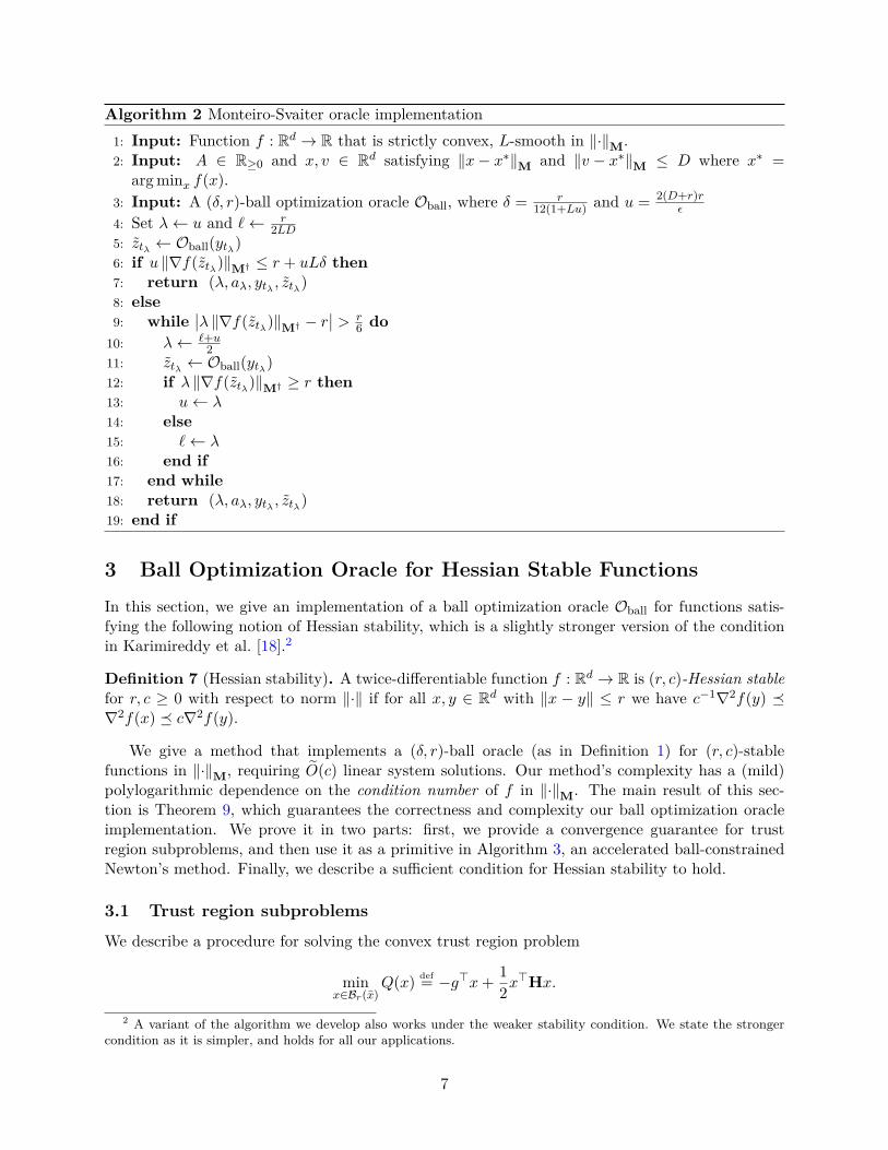
Algorithm 2 Monteiro-Svaiter oracle implementation1: Input: Function f : Rd → R that is strictly convex, L-smooth in ‖·‖M.2: Input: A ∈ R≥0 and x, v ∈ Rd satisfying ‖x− x∗‖M and ‖v − x∗‖M ≤ D where x∗ =

arg minx f(x).3: Input: A (δ, r)-ball optimization oracle Oball, where δ = r

12(1+Lu) and u = 2(D+r)rε

4: Set λ← u and `← r2LD

5: ztλ ← Oball(ytλ)6: if u ‖∇f(ztλ)‖M† ≤ r + uLδ then7: return (λ, aλ, ytλ , ztλ)8: else9: while

∣∣λ ‖∇f(ztλ)‖M† − r∣∣ > r

6 do10: λ← `+u

211: ztλ ← Oball(ytλ)12: if λ ‖∇f(ztλ)‖M† ≥ r then13: u← λ14: else15: `← λ16: end if17: end while18: return (λ, aλ, ytλ , ztλ)19: end if

3 Ball Optimization Oracle for Hessian Stable FunctionsIn this section, we give an implementation of a ball optimization oracle Oball for functions satis-fying the following notion of Hessian stability, which is a slightly stronger version of the conditionin Karimireddy et al. [18].2

Definition 7 (Hessian stability). A twice-differentiable function f : Rd → R is (r, c)-Hessian stablefor r, c ≥ 0 with respect to norm ‖·‖ if for all x, y ∈ Rd with ‖x − y‖ ≤ r we have c−1∇2f(y) ∇2f(x) c∇2f(y).

We give a method that implements a (δ, r)-ball oracle (as in Definition 1) for (r, c)-stablefunctions in ‖·‖M, requiring O(c) linear system solutions. Our method’s complexity has a (mild)polylogarithmic dependence on the condition number of f in ‖·‖M. The main result of this sec-tion is Theorem 9, which guarantees the correctness and complexity our ball optimization oracleimplementation. We prove it in two parts: first, we provide a convergence guarantee for trustregion subproblems, and then use it as a primitive in Algorithm 3, an accelerated ball-constrainedNewton’s method. Finally, we describe a sufficient condition for Hessian stability to hold.

3.1 Trust region subproblems

We describe a procedure for solving the convex trust region problem

minx∈Br(x)

Q(x) def= −g>x+ 12x>Hx.

2 A variant of the algorithm we develop also works under the weaker stability condition. We state the strongercondition as it is simpler, and holds for all our applications.

7

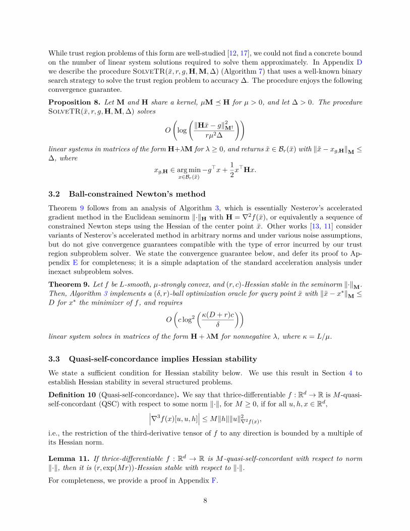
While trust region problems of this form are well-studied [12, 17], we could not find a concrete boundon the number of linear system solutions required to solve them approximately. In Appendix Dwe describe the procedure SolveTR(x, r, g,H,M,∆) (Algorithm 7) that uses a well-known binarysearch strategy to solve the trust region problem to accuracy ∆. The procedure enjoys the followingconvergence guarantee.

Proposition 8. Let M and H share a kernel, µM H for µ > 0, and let ∆ > 0. The procedureSolveTR(x, r, g,H,M,∆) solves

O

(log

(‖Hx− g‖2M†

rµ2∆

))linear systems in matrices of the form H+λM for λ ≥ 0, and returns x ∈ Br(x) with ‖x− xg,H‖M ≤∆, where

xg,H ∈ arg minx∈Br(x)

−g>x+ 12x>Hx.

3.2 Ball-constrained Newton’s method

Theorem 9 follows from an analysis of Algorithm 3, which is essentially Nesterov’s acceleratedgradient method in the Euclidean seminorm ‖·‖H with H = ∇2f(x), or equivalently a sequence ofconstrained Newton steps using the Hessian of the center point x. Other works [13, 11] considervariants of Nesterov’s accelerated method in arbitrary norms and under various noise assumptions,but do not give convergence guarantees compatible with the type of error incurred by our trustregion subproblem solver. We state the convergence guarantee below, and defer its proof to Ap-pendix E for completeness; it is a simple adaptation of the standard acceleration analysis underinexact subproblem solves.

Theorem 9. Let f be L-smooth, µ-strongly convex, and (r, c)-Hessian stable in the seminorm ‖·‖M.Then, Algorithm 3 implements a (δ, r)-ball optimization oracle for query point x with ‖x− x∗‖M ≤D for x∗ the minimizer of f , and requires

O

(c log2

(κ(D + r)c

δ

))linear system solves in matrices of the form H + λM for nonnegative λ, where κ = L/µ.

3.3 Quasi-self-concordance implies Hessian stability

We state a sufficient condition for Hessian stability below. We use this result in Section 4 toestablish Hessian stability in several structured problems.

Definition 10 (Quasi-self-concordance). We say that thrice-differentiable f : Rd → R is M -quasi-self-concordant (QSC) with respect to some norm ‖·‖, for M ≥ 0, if for all u, h, x ∈ Rd,∣∣∣∇3f(x)[u, u, h]

∣∣∣ ≤M‖h‖‖u‖2∇2f(x),

i.e., the restriction of the third-derivative tensor of f to any direction is bounded by a multiple ofits Hessian norm.

Lemma 11. If thrice-differentiable f : Rd → R is M -quasi-self-concordant with respect to norm‖·‖, then it is (r, exp(Mr))-Hessian stable with respect to ‖·‖.

For completeness, we provide a proof in Appendix F.

8

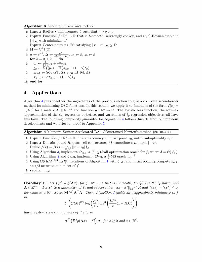
Algorithm 3 Accelerated Newton’s method1: Input: Radius r and accuracy δ such that r ≥ δ > 0.2: Input: Function f : Rd → R that is L-smooth, µ-strongly convex, and (r, c)-Hessian stable in‖·‖M with minimizer x∗.

3: Input: Center point x ∈ Rd satisfying ‖x− x∗‖M ≤ D.4: H← ∇2f(x)5: α← c−1, ∆← µδ2

4Lc(5r+D) , x0 ← x, z0 ← x6: for k = 0, 1, 2, . . . do7: yk ← 1

1+αxk + α1+αzk

8: gk ← ∇f(yk)−H(αyk + (1− α)zk)9: zk+1 ← SolveTR(x, r, gk,H,M,∆)

10: xk+1 ← αzk+1 + (1− α)xk11: end for

4 ApplicationsAlgorithm 4 puts together the ingredients of the previous section to give a complete second-ordermethod for minimizing QSC functions. In this section, we apply it to functions of the form f(x) =g(Ax) for a matrix A ∈ Rn×d and function g : Rn → R. The logistic loss function, the softmaxapproximation of the `∞ regression objective, and variations of `p regression objectives, all havethis form. The following complexity guarantee for Algorithm 4 follows directly from our previousdevelopments and we defer its proof to Appendix G.

Algorithm 4 Monteiro-Svaiter Accelerated BAll COnstrained Newton’s method (MS-BACON)1: Input: Function f : Rd → R, desired accuracy ε, initial point x0, initial suboptimality ε0.2: Input: Domain bound R, quasi-self-concordance M , smoothness L, norm ‖·‖M.3: Define f(x) = f(x) + ε

55R2 ‖x− x0‖2M4: Using Algorithm 3, implement Oball, a (δ, 1

M )-ball optimization oracle for f , where δ = Θ( εLR)

5: Using Algorithm 2 and Oball, implement OMS, a 12 -MS oracle for f

6: Using O((RM)2/3 log ε0ε ) iterations of Algorithm 1 with OMS and initial point x0 compute xout,

an ε/2-accurate minimizer of f7: return xout

Corollary 12. Let f(x) = g(Ax), for g : Rn → R that is L-smooth, M -QSC in the `2 norm, andA ∈ Rn×d. Let x∗ be a minimizer of f , and suppose that ‖x0 − x∗‖M ≤ R and f(x0)− f(x∗) ≤ ε0for some x0 ∈ Rd, where M def= A>A. Then, Algorithm 4 yields an ε-approximate minimizer to fin

O

((RM)2/3 log

(ε0ε

)log3

(LR2

ε(1 +RM)

))linear system solves in matrices of the form

A>(∇2g(Ax) + λI

)A for λ ≥ 0 and x ∈ Rd.

9

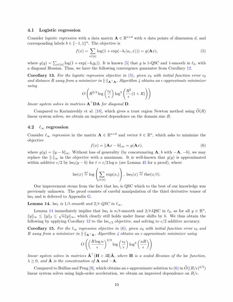
4.1 Logistic regression

Consider logistic regression with a data matrix A ∈ Rn×d with n data points of dimension d, andcorresponding labels b ∈ −1, 1n. The objective is

f(x) =∑i∈[n]

log(1 + exp(−bi〈ai, x〉)) = g(Ax), (5)

where g(y) =∑i∈[n] log(1 + exp(−biyi)). It is known [5] that g is 1-QSC and 1-smooth in `2, with

a diagonal Hessian. Thus, we have the following convergence guarantee from Corollary 12.

Corollary 13. For the logistic regression objective in (5), given x0 with initial function error ε0and distance R away from a minimizer in ‖·‖A>A, Algorithm 4 obtains an ε-approximate minimizerusing

O

(R2/3 log

(ε0ε

)log3

(R2

ε(1 +R)

))linear system solves in matrices A>DA for diagonal D.

Compared to Karimireddy et al. [18], which gives a trust region Newton method using O(R)linear system solves, we obtain an improved dependence on the domain size R.

4.2 `∞ regression

Consider `∞ regression in the matrix A ∈ Rn×d and vector b ∈ Rn, which asks to minimize theobjective

f(x) = ‖Ax− b‖∞ = g(Ax), (6)where g(y) = ‖y − b‖∞. Without loss of generality (by concatenating A, b with −A, −b), we mayreplace the ‖·‖∞ in the objective with a maximum. It is well-known that g(y) is approximatedwithin additive ε/2 by lset(y − b) for t = ε/2 logn (see Lemma 45 for a proof), where

lse(x) def= log

∑i∈[n]

exp(xi)

, lset(x) def= tlse(x/t).

Our improvement stems from the fact that lset is QSC which to the best of our knowledge waspreviously unknown. The proof consists of careful manipulation of the third derivative tensor oflset and is deferred to Appendix G.

Lemma 14. lset is 1/t-smooth and 2/t-QSC in `∞.

Lemma 14 immediately implies that lset is n/t-smooth and 2/t-QSC in `2, as for all y ∈ Rn,‖y‖∞ ≤ ‖y‖2 ≤

√n‖y‖∞, which clearly still holds under linear shifts by b. We thus obtain the

following by applying Corollary 12 to the lseε/2 objective, and solving to ε/2 additive accuracy.

Corollary 15. For the `∞ regression objective in (6), given x0 with initial function error ε0 andR away from a minimizer in ‖·‖A>A, Algorithm 4 obtains an ε-approximate minimizer using

O

((R lognε

)2/3log

(ε0ε

)log3

(nR

ε

))

linear system solves in matrices A>(H + λI)A, where H is a scaled Hessian of the lse function,λ ≥ 0, and A is the concatenation of A and −A.

Compared to Bullins and Peng [9], which obtains an ε-approximate solution to (6) in O((R/ε)4/5)linear system solves using high-order acceleration, we obtain an improved dependence on R/ε.

10

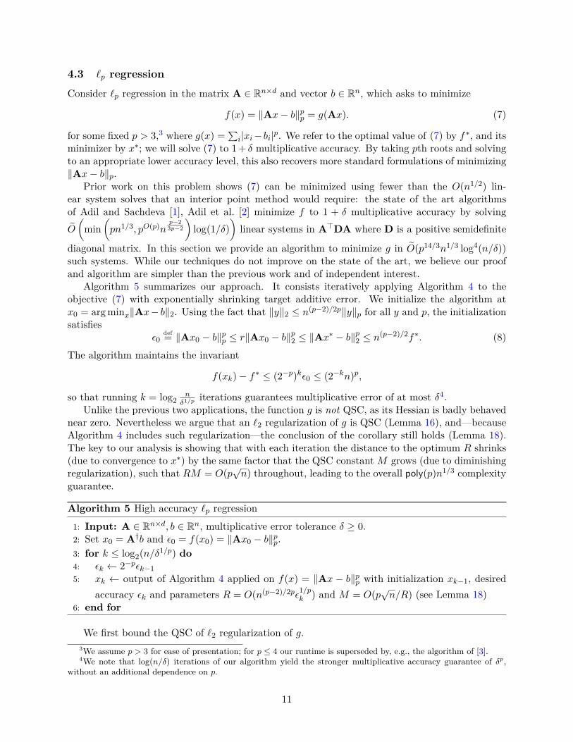
4.3 `p regression

Consider `p regression in the matrix A ∈ Rn×d and vector b ∈ Rn, which asks to minimize

f(x) = ‖Ax− b‖pp = g(Ax). (7)

for some fixed p > 3,3 where g(x) =∑i|xi−bi|p. We refer to the optimal value of (7) by f∗, and its

minimizer by x∗; we will solve (7) to 1 + δ multiplicative accuracy. By taking pth roots and solvingto an appropriate lower accuracy level, this also recovers more standard formulations of minimizing‖Ax− b‖p.

Prior work on this problem shows (7) can be minimized using fewer than the O(n1/2) lin-ear system solves that an interior point method would require: the state of the art algorithmsof Adil and Sachdeva [1], Adil et al. [2] minimize f to 1 + δ multiplicative accuracy by solvingO

(min

(pn1/3, pO(p)n

p−23p−2

)log(1/δ)

)linear systems in A>DA where D is a positive semidefinite

diagonal matrix. In this section we provide an algorithm to minimize g in O(p14/3n1/3 log4(n/δ))such systems. While our techniques do not improve on the state of the art, we believe our proofand algorithm are simpler than the previous work and of independent interest.

Algorithm 5 summarizes our approach. It consists iteratively applying Algorithm 4 to theobjective (7) with exponentially shrinking target additive error. We initialize the algorithm atx0 = arg minx‖Ax− b‖2. Using the fact that ‖y‖2 ≤ n(p−2)/2p‖y‖p for all y and p, the initializationsatisfies

ε0def= ‖Ax0 − b‖pp ≤ r‖Ax0 − b‖p2 ≤ ‖Ax∗ − b‖

p2 ≤ n

(p−2)/2f∗. (8)

The algorithm maintains the invariant

f(xk)− f∗ ≤ (2−p)kε0 ≤ (2−kn)p,

so that running k = log2nδ1/p iterations guarantees multiplicative error of at most δ4.

Unlike the previous two applications, the function g is not QSC, as its Hessian is badly behavednear zero. Nevertheless we argue that an `2 regularization of g is QSC (Lemma 16), and—becauseAlgorithm 4 includes such regularization—the conclusion of the corollary still holds (Lemma 18).The key to our analysis is showing that with each iteration the distance to the optimum R shrinks(due to convergence to x∗) by the same factor that the QSC constant M grows (due to diminishingregularization), such that RM = O(p

√n) throughout, leading to the overall poly(p)n1/3 complexity

guarantee.

Algorithm 5 High accuracy `p regression

1: Input: A ∈ Rn×d, b ∈ Rn, multiplicative error tolerance δ ≥ 0.2: Set x0 = A†b and ε0 = f(x0) = ‖Ax0 − b‖pp.3: for k ≤ log2(n/δ1/p) do4: εk ← 2−pεk−15: xk ← output of Algorithm 4 applied on f(x) = ‖Ax − b‖pp with initialization xk−1, desired

accuracy εk and parameters R = O(n(p−2)/2pε1/pk ) and M = O(p

√n/R) (see Lemma 18)

6: end for

We first bound the QSC of `2 regularization of g.3We assume p > 3 for ease of presentation; for p ≤ 4 our runtime is superseded by, e.g., the algorithm of [3].4We note that log(n/δ) iterations of our algorithm yield the stronger multiplicative accuracy guarantee of δp,

without an additional dependence on p.

11

Lemma 16. For any b ∈ Rn, y ∈ Rd, p ≥ 3, µ ≥ 0, the function g(x)+µ‖x−y‖22 is O(pµ−1/(p−2))-QSC with respect to `2.

We next show approximate minimizers of f are close to x∗.

Lemma 17. For x ∈ Rd with f(x)− f∗ ≤ ε, we have ‖x− x∗‖pM ≤ 2pnp−2

2 ε.

Finally, we bound the complexity of executions of Line 5.

Lemma 18. Let εk−1 ≥ δf∗. Initialized at xk−1 satisfying f(xk−1) − f∗ ≤ εk−1, Algorithm 4computes xk with f(xk) − f∗ ≤ 2−pεk−1 = εk in O(p14/3n1/3 log3(n/δ)) linear system solves inA>DA for diagonal matrix D 0.

We defer proofs of these statements to Appendix G.2. Our final runtime follows from Lemma 18and the fact that the loop in Algorithm 5 repeats O(log n

δ ) times.

Corollary 19. Algorithm 5 computes x ∈ Rd with

‖Ax− b‖pp ≤ (1 + δ)‖Ax∗ − b‖pp

using O(p14/3n1/3 log4(n/δ)) linear system solves in A>DA for diagonal matrix D 0.

5 Lower boundIn this section we establish a lower bound showing that the (R/r)2/3 scaling in the oracle complexitywe achieve is tight. For simplicity, we focus on a setting where the functions are defined on abounded domain of radius R > 0, and are 1-Lipschitz but potentially non-smooth; afterwards, weexplain how to extend the result to unconstrained, differentiable and strictly convex functions. Weassume throughout the section that M = I, i.e., that we work in the standard `2 norm. We deferall the proofs in this section to Appendix H.

Following the literature on information-based complexity [21], we state and prove our lowerbound for the class of r-local oracles, which for every query point x return a function fx thatis identical to f in a neighborhood of x. However, we additionally require the radius of thisneighborhood to be at least r. Therefore, a query to an r-local oracle suffices to implement a balloptimization oracle (as well as a gradient oracle), and consequently a lower bound on algorithmsinteracting with an r-local oracles is also a lower bounds for algorithms a utilizing ball optimizationoracle. The formal definition of the oracle class follows.

Definition 20 (Local oracles and algorithms). We call Olocal an r-local oracle for function f :BR(0) → R if given query point x ∈ Rd it returns fx : BR(0) → R such that fx(x) = f(x) forall x ∈ Br(x). We call (possibly randomized) algorithms that interact with r-local oracles r-localalgorithms.

We prove our lower bound using a small extension of the well-established machinery of high-dimensional optimization lower bounds [21, 24, 10, 8]. To describe it, we start with the notion ofcoordinate progress, denoting for any x ∈ Rd

i+r (x) def= mini ∈ [d] | |xj | ≤ r for all j ≥ i, (9)

where we let i+r (x) def= d+ 1 when |xd| > r, i.e. i+r (x) is the index following the last “large” entry ofx. With this notation, we define a key notion for proving our lower bound.

12

Definition 21 (Robust zero-chains). Function f : B1(0)→ R is an r-robust zero-chain if ∀x ∈ Rd,x ∈ Br(x),

f(x) = f(x1, . . . , xi+r (x), 0, . . . , 0).

The notion of r-robust zero-chain we use here is very close to the robust zero-chain definedin [10, Definition 4], except here we require the equality to hold in a fixed ball rather than justa neighborhood of x. The following lemma shows that r-local algorithms operating on a randomrotation of an r-robust zero-chain make slow progress with high probability.5

Lemma 22. Let rR , δ ∈ (0, 1), N ∈ N and d ≥

⌈N + 20R2

r2 log 20NR2

δr2⌉. Let f : BR(0) → R

be an r-robust zero-chain and let U ∈ Rd×d be a random orthogonal matrix and fix an r-localalgorithm A. With probability at least 1− δ over the draw of U, there exists an r-local oracle O forfU(x) def= f(U>x) such that the queries x1, x2, . . . of A interacting with O satisfy

i+r (U>xi) ≤ i for all i ≤ N.

With Lemma 22 in hand, to prove the lower bound we need to construct an r-robust zero-chainfunction fN,r with the additional property that every x with i+r (x) ≤ N is significantly suboptimal.Fortunately, Nemirovski’s function [21] satisfies these properties.

Lemma 23. Let r > 0 and N ∈ N. Define

fN,r(x) def= maxi∈[N ]xi − 4r · i (10)

1. The function fN,r is an r-robust zero-chain.

2. For all x ∈ BR(0) such that i+r (x) ≤ N , we have fN,r(x)− infz∈BR(0) fN,r(z) ≥ R√N− 4Nr.

3. The function fN,r is convex and 1-Lipschitz.

Lemma 23.1 is the main technical novelty of the section, while the other parts are knownand stated for completeness. Combining Lemmas 22 and 23 with appropriate choices of N and dimmediately gives the lower bound.

Theorem 24. Let rR , δ ∈ (0, 1) and d =

⌈60(Rr )2 log R

δ·r⌉. There exists a distribution P over convex

and 1-Lipschitz functions from BR(0)→ R and corresponding r-local oracles such that the followingholds for any r-local algorithm. With probability at least 1 − δ over the draw of (f,O) ∼ P , whenthe algorithm interacts with O, its first

⌈ 110(Rr )2/3⌉ queries are at least R2/3r1/3 suboptimal for f .

Proof. Set N =⌊

110(Rr )2/3

⌋and d ≥

⌈60R2

r2 log Rδr

⌉≥⌈N + 20R2

r2 log 20NR2

δr2

⌉. Apply Lemma 22 with

Lemma 23.1 to argue that for any r-local algorithm, with probability at least 1 − δ the first Nqueries x1, . . . , xN satisfy i+r (U>xi) ≤ N , and substitute into Lemma 23.2 to conclude that thesuboptimality of each query is at least (

√10− 4

10)(R2r)1/3 ≥ (R2r)1/3.

Theorem 24 shows as long as we wish to solve the minimization problem to accuracy ε =o(R2/3r1/3), for any r-local algorithm, there is a function requiring Ω((R/r)2/3) queries to an r-localoracle, which gives strictly more information than a ball optimization oracle, proving our desiredlower bound. However, our acceleration scheme assumes unconstrained, smooth and strictly convexproblems. We now outline modifications to the construction (10) extending it to this regime.

5 In Appendix H we provide a concise proof for Lemma 22 and compare it to existing proofs in the literature.

13

Unconstrained domain. Following the approach of Diakonikolas and Guzmán [14], we notethat the construction f(x) = max1

2fN,r(x), ‖x‖ − R2 provides a hard instance for algorithms

with unbounded queries, because any query with norm larger than ‖x‖ is uninformative about therotation of coordinates and has a positive function value, so that the minimizer is still constrainedto a ball of radius R.

Smooth functions. The smoothing argument of Guzmán and Nemirovski [16] shows that f(x) =infx′∈Br(x)fN,2r(x′) + 1

r‖x′ − x‖2 is an r-robust zero-chain that is also 2/r-smooth and satisfies

|f(x)− fN,2r(x)| ≤ r for all x. Consequently, the lower bound holds for O(1/r) smooth functions.

Strictly convex functions. The function f(x) = fN,r(x) + r1/3

2R4/3 ‖x‖2 provides an (r1/3R−4/3)-strongly convex hard instance, since we can add the strongly convex regularizer directly in the localoracle without revealing additional information, and the regularizer size is small enough so as notto significantly affect the optimality gap.

References[1] Deeksha Adil and Sushant Sachdeva. Faster p-norm minimizing flows, via smoothed q-norm

problems. In Symposium on Discrete Algorithms, SODA, pages 892–910, 2020.

[2] Deeksha Adil, Rasmus Kyng, Richard Peng, and Sushant Sachdeva. Iterative refinement for`p-norm regression. In Symposium on Discrete Algorithms, SODA, pages 1405–1424, 2019.

[3] Deeksha Adil, Richard Peng, and Sushant Sachdeva. Fast, provably convergent IRLS algorithmfor p-norm linear regression. In Advances in Neural Information Processing Systems, NeurIPS,pages 14166–14177, 2019.

[4] Naman Agarwal, Brian Bullins, and Elad Hazan. Second-order stochastic optimization formachine learning in linear time. Journal of Machine Learning Research, 18(1):4148–4187,2017.

[5] Francis Bach et al. Self-concordant analysis for logistic regression. Electronic Journal ofStatistics, 4:384–414, 2010.

[6] Keith Ball et al. An elementary introduction to modern convex geometry. Flavors of geometry,31:1–58, 1997.

[7] Sébastien Bubeck, Michael B. Cohen, Yin Tat Lee, and Yuanzhi Li. An homotopy method for`p regression provably beyond self-concordance and in input-sparsity time. In Symposium onTheory of Computing, STOC, pages 1130–1137, 2018.

[8] Sébastien Bubeck, Qijia Jiang, Yin-Tat Lee, Yuanzhi Li, and Aaron Sidford. Complexity ofhighly parallel non-smooth convex optimization. In Advances in Neural Information ProcessingSystems, pages 13900–13909, 2019.

[9] Brian Bullins and Richard Peng. Higher-order accelerated methods for faster non-smoothoptimization. arXiv preprint arXiv:1906.01621, 2019.

[10] Yair Carmon, John C Duchi, Oliver Hinder, and Aaron Sidford. Lower bounds for findingstationary points I. Mathematical Programming, May 2019.

14

[11] Michael Cohen, Jelena Diakonikolas, and Lorenzo Orecchia. On acceleration with noise-corrupted gradients. In Proceedings of the 35th International Conference on Machine Learning,ICML 2018, Stockholmsmässan, Stockholm, Sweden, July 10-15, 2018, pages 1018–1027, 2018.

[12] Andrew R. Conn, Nicholas I. M. Gould, and Philippe L. Toint. Trust Region Methods. MOS-SIAM Series on Optimization. SIAM, 2000.

[13] Olivier Devolder, François Glineur, and Yurii E. Nesterov. First-order methods of smoothconvex optimization with inexact oracle. Math. Program., 146(1-2):37–75, 2014.

[14] Jelena Diakonikolas and Cristóbal Guzmán. Lower bounds for parallel and randomized convexoptimization. In Conference on Learning Theory, COLT, pages 1132–1157, 2019.

[15] Alexander Gasnikov, Pavel E. Dvurechensky, Eduard A. Gorbunov, Evgeniya A. Vorontsova,Daniil Selikhanovych, César A. Uribe, Bo Jiang, Haoyue Wang, Shuzhong Zhang, SébastienBubeck, Qijia Jiang, Yin Tat Lee, Yuanzhi Li, and Aaron Sidford. Near optimal methodsfor minimizing convex functions with lipschitz p-th derivatives. In Conference on LearningTheory, COLT 2019, pages 1392–1393, 2019.

[16] Cristóbal Guzmán and Arkadi Nemirovski. On lower complexity bounds for large-scale smoothconvex optimization. Journal of Complexity, 31(1):1–14, 2015.

[17] William W. Hager. Minimizing a quadratic over a sphere. SIAM Journal on Optimization, 12(1):188–208, 2001.

[18] Sai Praneeth Karimireddy, Sebastian U Stich, and Martin Jaggi. Global linear conver-gence of Newton’s method without strong-convexity or lipschitz gradients. arXiv preprintarXiv:1806.00413, 2018.

[19] Chih-Jen Lin, Ruby C. Weng, and S. Sathiya Keerthi. Trust region Newton method for large-scale logistic regression. Journal of Machine Learning Research, 9:627–650, 2008.

[20] Renato D. C. Monteiro and Benar Fux Svaiter. An accelerated hybrid proximal extragradientmethod for convex optimization and its implications to second-order methods. SIAM Journalon Optimization, 23(2):1092–1125, 2013.

[21] Arkadi Nemirovski and David Borisovich Yudin. Problem Complexity and Method Efficiencyin Optimization. Wiley, 1983.

[22] Yurii Nesterov. A method for solving a convex programming problem with convergence rateo(1/k2). Doklady AN SSSR, 269:543–547, 1983.

[23] Mark Schmidt, Dongmin Kim, and Suvrit Sra. Projected Newton-type methods in machinelearning. In Suvrit Sra, Sebastian Nowozin, and Stephen J Wright, editors, Optimization forMachine Learning, chapter 11. MIT Press, 2011.

[24] Blake Woodworth and Nathan Srebro. Tight complexity bounds for optimizing compositeobjectives. In Advances in neural information processing systems, pages 3639–3647, 2016.

[25] Blake Woodworth and Nathan Srebro. Lower bound for randomized first order convex opti-mization. arXiv preprint arXiv:1709.03594, 2017.

[26] Andrew Chi-Chin Yao. Probabilistic computations: Toward a unified measure of complexity.In 18th Annual Symposium on Foundations of Computer Science, pages 222–227, 1977.

15

Supplementary materialA Unaccelerated optimization with a ball optimization oracleHere, we state and analyze the unaccelerated algorithm for optimization of convex function f withaccess to a ball optimization oracle. For simplicity of exposition, we assume that the oracle Oballis a (0, r)-oracle, i.e. is exact, and we perform our analysis in the `2 norm; for a general Euclideanseminorm, a change of basis suffices to give the same guarantees.

Algorithm 6 Iterating ball optimization1: Input: Function f : Rd → R and initial point x0 ∈ Rd.2: for k = 1, 2, ... do3: xk ← Oball(xk−1)4: end for

We first note that the distance ‖xk − x∗‖2 is decreasing in k.

Lemma 25. For all x ∈ Rd, ‖Oball(x)− x∗‖2 ≤ ‖x− x∗‖2.

Proof. The claim is obvious if Oball(x) = x∗, so we assume this is not the case. Note that for anyx with ‖x− x‖2 ≤ r, if there is any point x on the line between x and x∗, then by strict convexityf(x) < f(x). Now, clearlyOball(x) lies on the boundary of the ball around x, and moreover the anglebetween the vectors x−Oball(x) and x∗−Oball(x) must be obtuse, else the line between Oball(x) andx∗ intersects the ball twice. Thus, by law of cosines ‖Oball(x)− x∗‖2 ≤

√‖x− x∗‖22 − r2, yielding

the conclusion.

Theorem 26. Suppose for some x0 ∈ Rd, f(x0)− f(x∗) ≤ ε0 and ‖x0− x∗‖2 ≤ R, where x∗ is theglobal minimizer of f . Algorithm 6 computes an ε-approximate minimizer in O

(Rr log ε0

ε

)calls to

Oball.

Proof. Define xkdef=(1− r

R

)xk−1 + r

Rx∗, and note that because ‖xk−1− x∗‖2 ≤ R, xk is in the ball

of radius r around xk−1. Thus, convexity yields

f(xk) ≤ f(xk) ≤(

1− r

R

)f(xk−1) + r

Rf(x∗)⇒ f(xk)− f(x∗) ≤

(1− r

R

)(f(xk−1)− f(x∗)) .

Iteratively applying this inequality yields the conclusion.

B Analysis of Monteiro-Svaiter accelerationIn this section, we prove Proposition 3. We do so by first proving a sequence of lemmas demon-strating properties of Algorithm 1. Throughout, we recall ∇f(x) ∈ Im(M) for all x by assumption.We note that these are variants of existing bounds in the literature [e.g. 20, 8].

Lemma 27. For all k ≥ 0,

λk+1Ak+1 = a2k+1 and

√Ak ≥

12∑i∈[k]

√λi.

16

Proof. The first claim is from solving a quadratic in the definition of ak+1. The second follows from√Ak ≥

√Ak −

√A0 =

∑i∈[k]

(√Ai −

√Ai−1

)=∑i∈[k]

ai√Ai +

√Ai−1

=∑i∈[k]

√λiAi√

Ai +√Ai−1

≥ 12∑i∈[k]

√λi

where we used that A0 ≥ 0 and Ai are increasing.

Lemma 28. For all k ≥ 0, if ‖xk+1 − yk‖M > 0, we have for σ ∈ [0, 1),

‖∇f(xk+1)‖M† > 0 and λk+1 ≥‖xk+1 − yk‖M‖∇f(xk+1)‖M†

(1− σ) > 0 .

Proof. For the first claim, by (3),

‖xk+1 − yk‖M − λk+1‖∇f(xk+1)‖M† ≤ ‖xk+1 − (yk − λk+1M†∇f(xk+1))‖M ≤ σ‖xk+1 − yk‖M,

since by assumption, for some σ ∈ [0, 1), ‖xk+1 − yk‖M > 0, therefore ‖∇f(xk+1)‖M† = 0 wouldcontradict this assumption.

For the second claim, Cauchy-Schwarz gives

σ2 ‖xk+1 − yk‖2M ≥∥∥∥xk+1 −

(yk − λk+1M†∇f(xk+1)

)∥∥∥2

M

≥ ‖xk+1 − yk‖2M − 2λk+1‖∇f(xk+1)‖M†‖xk+1 − yk‖M + λ2k+1‖∇f(xk+1)‖2M† .

Solving the quadratic in λk+1 implies, for P def= ‖∇f(xk+1)‖M†‖xk+1 − yk‖M,

λk+1 ≥2P −

√4P 2 − 4(1− σ2)P 2

2‖∇f(xk+1)‖2M†= P (1− σ)‖∇f(xk+1)‖2M†

= ‖xk+1 − yk‖M‖∇f(xk+1)‖M†

(1− σ) .

Next, we provide the following lemma which gives a recursive bound for the potential, pk, whichwe define as follows:

pkdef= Akεk + rk, where εk

def= f(xk)− f(x∗), rkdef= 1

2 ‖vk − x∗‖2M .

We remark that the proof does not use (3) beyond using the property that ak+1 > 0 (regardless ofhow they are induced by λk+1).

Lemma 29. For all k ≥ 0,

pk+1 ≤ pk +A2k+1

2a2k+1

∥∥∥∥∥xk+1 −(yk −

a2k+1Ak+1

M†∇f(xk+1))∥∥∥∥∥

2

M− ‖xk+1 − yk‖2M

.Proof. By Lemma 28 we have that λk+1 > 0, so that ak+1 > 0. Then,

vk = 1ak+1

(Ak+1yk −Akxk) = xk+1 + Ak+1ak+1

(yk − xk+1) + Akak+1

(xk+1 − xk).

17

Consequently, convexity of f , i.e., 〈∇f(b), a− b〉 ≤ f(a)− f(b) for all a, b ∈ Rn, yields

ak+1 〈∇f(xk+1), x∗ − vk〉 ≤ Akεk −Ak+1εk+1 +Ak+1 〈∇f(xk+1), xk+1 − yk〉 .

Further, expanding rk+1 = 12 ‖vk+1 − x∗‖2M, where we recall vk+1 = vk − ak+1M†∇f(xk+1), gives

12 ‖vk+1 − x∗‖2M = rk +

a2k+12 ‖∇f(xk+1)‖2M† + ak+1

⟨MM†∇f(xk+1), x∗ − vk

⟩.

Combining these inequalities, and recalling MM†∇f(xk+1) = ∇f(xk+1), then yields that

Ak+1εk+1 + rk+1 ≤ Akεk + rk +a2k+12 ‖∇f(xk+1)‖2M† +Ak+1 〈∇f(xk+1), xk+1 − yk〉 .

The result then follows from pk = Akεk + rk and the fact that

A2k+1

2a2k+1

∥∥∥∥∥xk+1 −(yk −

a2k+1Ak+1

M†∇f(xk+1))∥∥∥∥∥

2

M

=A2k+1

2a2k+1‖xk+1 − yk‖2M +Ak+1 〈∇f(xk+1), xk+1 − yk〉+

a2k+12 ‖∇f(xk+1)‖2M† .

Next, we use (3) and the choice of ak+1 in the algorithm to improve the bound in Lemma 29.

Lemma 30. For all k ≥ 0,

pk +∑i∈[k]

(1− σ2)Ai2λi

‖xi+1 − yi‖2M ≤ p0 .

Proof. Lemma 27 gives that for our choice of parameters, λk+1Ak+1 = a2k+1 for all k ≥ 0. Lemma 29

then implies that

Ak+1εk+1 + rk+1 ≤ Akεk + rk + Ak+12λk+1

(∥∥∥xk+1 −(yk − λk+1M†∇f(xk+1)

)∥∥∥2

M− ‖xk+1 − yk‖2M

)≤ Akεk + rk + (σ2 − 1)Ak+1

2λk+1‖xk+1 − yk‖2M

where we used (3) and the claim now follows from inductively applying the resulting bound.

Below we give a diameter bound on the iterates from the algorithm.

Lemma 31. If x0 = v0, then for all k ≥ 0 we have

‖xk − x∗‖M ≤2− σ1− σ

√2p0, ‖vk − x∗‖M ≤

√2p0.

Proof. Since pk = Akεk + rk, the second claim follows immediately from Lemma 30 implying that12 ‖vk − x

∗‖2M = rk ≤ p0 for all k ≥ 0. Further, convexity and the triangle inequality imply that

‖xk+1 − x∗‖M ≤ ‖yk − x∗‖M + ‖xk+1 − yk‖M

≤ AkAk+1

‖xk − x∗‖M + ak+1Ak+1

‖vk − x∗‖M + ‖xk+1 − yk‖M .

18

Rearranging and applying recursively yields that

Ak+1 ‖xk+1 − x∗‖M ≤ Ak ‖xk − x∗‖M + ak+1 ‖vk − x∗‖M +Ak+1 ‖xk+1 − yk‖M

≤ A0 ‖x0 − x∗‖M +k∑i=0

ai+1 ‖vi − x∗‖M +k∑i=0

Ai+1 ‖xi+1 − yi‖M .

Now, using Ak+1 = A0 +∑ki=0 ai+1, x0 = v0, the previously-derived ‖vi − x∗‖M ≤

√2p0, and

Cauchy-Schwarz,

‖xk+1 − x∗‖M ≤√

2p0 + 1Ak+1

√√√√( k∑i=0

λi+1Ai+1

)(k∑i=0

Ai+1λi+1

‖xi+1 − yi‖2M

).

Now, since λk+1Ak+1 = a2k+1 and

√a+ b ≤

√a+√b for nonnegative a, b we have√√√√ k∑

i=0λi+1Ai+1 ≤

k∑i=0

√λi+1Ai+1 =

k∑i=0

ai+1 = Ak+1,

and the result follows fromk∑i=0

Ai+1λi+1

‖xi+1 − yi‖2M ≤ (1− σ2)−12p0

(due to Lemma 30), and√

(1− σ2)−1 ≤ (1− σ)−1.

We next give a basic helper lemma which will be useful in the proof of Proposition 3.

Lemma 32. Let Bkk∈N be a nonnegative, nondecreasing sequence such that Bk ≥∑i∈[k] αBi for

some α ∈ [0, 1) and all k. Then for all k, Bk ≥ exp(α(k − 1))B1.

Proof. Extend C(t) def= Bdte for all t ≥ 1, and let C(t) def= exp(α(t− 1))B1 for t ∈ [0, 1]. Then for allt ≥ 1,

C(t) = Bdte ≥ α∑i∈[dte]

Bi ≥ α∫ t

0C(s)ds,

and it is easy to check that this inequality holds with equality for t ∈ [0, 1] as well. Letting L(t)solve this integral inequality, i.e., L(t) = C(t) for t ∈ [0, 1] and

L(t) = α

∫ t

0L(s)ds,

L(t) = exp(α(t − 1))C(1), and inequality C(t) ≥ L(t) yields the claim, recalling Bk = C(k) fork ∈ N.

Now we are ready to put everything together and prove the main result of this section.

Proposition 3. Let f be strictly convex and differentiable, with ‖x0 − x∗‖M ≤ R and f(x0) −f(x∗) ≤ ε0. Set A0 = R2/(2ε0) and suppose that for some r > 0 the iterates of Algorithm 1 satisfy

‖xk+1 − yk‖M ≥ r for all k ≥ 0.

Then, the iterates also satisfy

f(xk)− f(x∗) ≤ 2ε0 exp(−(r(1− σ)

R

)2/3(k − 1)

)·

19

Proof. First, we will show the bound

f(xk)− f(x∗) ≤ p0A1

exp

−32

(r(1− σ)√p0

)2/3

(k − 1)

. (11)

The reverse Hölder inequality with p = 3/2 states that for all u, v ∈ Rk>0,

〈u, v〉 ≥

∑i∈[k]

u2/3i

3/2

·

∑i∈[k]

v−2i

−1/2

. (12)

Lemma 27 gives√Ak ≥ 1

2∑i∈[k]√λi. Moreover, ‖xi − yi−1‖M > 0 by the assumptions of this

proposition, which implies by Lemma 28 that Ai ≥ λi > 0 as well. Thus, we can apply (12) withui =

√Ai‖xi − yi−1‖M and vi =

√λi/ui, yielding

√Ak ≥

12∑i∈[k]

√λi ≥

12

∑i∈[k]

(√Ai‖xi − yi−1‖M

)2/33/2∑

i∈[k]

( √λi√

Ai‖xi − yi−1‖M

)−2−1/2

.

(13)Applying Lemma 30 yields that

∑i∈[k]

( √λi√

Ai‖xi − yi−1‖M

)−2

=∑i∈[k]

Ai‖xi − yi−1‖2Mλi

≤( 2

1− σ2

)p0. (14)

Now, since ‖xi − yi−1‖M ≥ r by assumption, combining (13) and (14) gives

A1/3k ≥

(12

)2/3∑i∈[k]

A1/3i r2/3

(( 21− σ2

)p0

)−1/3=∑i∈[k]

A1/3i

(r2(1− σ2)

8p0

)1/3

.

Finally, applying Lemma 32 implies that for all k ≥ 0

Ak ≥ exp

32

(r2(1− σ2)

p0

)1/3

(k − 1)

A1.

Now, (11) follows from εk ≤ pk/Ak ≤ p0/Ak (we have pk ≤ p0 from Lemma 30) and (1 − σ2) ≤(1− σ)2. Now, by our choice of A0 = R2/2ε0, we have p0 = R2. As A1 ≥ A0,

p0A1≤ R2

A0= 2ε0.

Combining these bounds in the context of (11), and using 3/2 > 1, yields the result.

C MS oracle implementation proofsFirst, we prove our characterization of the optimizer of a ball-constrained problem.

Lemma 4. Let f : Rd → R be continuously differentiable and strictly convex. For all y ∈ Rd,

z = arg minz′∈Br(y)

f(z′)

is either the global minimizer of f , or ‖z − y‖M = r and ∇f(z) = −‖∇f(z)‖M†r M(z − y).

20

Proof. By considering the optimality conditions of the Lagrange dual problem

minz

maxλ≥0

f(z) + λ

2(‖z − y‖2M − r

2),

we see there is some λ ≥ 0 such that

∇f(z) = −λ∇z

(12 ‖z − y‖

2M −

r2

2

)= −λM(z − y) .

If λ = 0 then ∇f(z) = 0 and z is a minimizer of f . On the other hand, if λ > 0, then ‖z− y‖M = rand∇f(z) = −λM(z−y). By taking the M† seminorm of both sides of this condition, ‖∇f(z)‖M† =λ ‖z − y‖M = λr; solving for λ and substituting yields the result.

Next, on the path to proving Proposition 5, we give a helper result which bounds the changein the solution to a ball-constrained problem as we move the center.

Lemma 33. For strictly convex, twice differentiable f : Rd → R, let M be a positive semidefinitematrix where ∇f(u) ∈ Im(M) for all u ∈ Rd. Let x, v ∈ Rd be arbitrary vectors, and for allt ∈ [0, 1], let

ytdef= tx+ (1− t)v, zt

def= arg minz∈Br(yt)

f(z).

Then, for all t ∈ [0, 1] we have∥∥∥∥ ddtzt∥∥∥∥∇2f(zt)

=∥∥∥∥ ddt∇f(zt)

∥∥∥∥(∇2f(zt))−1

≤ ‖x− v‖∇2f(zt).

Proof. Let t ∈ [0, 1] be arbitrary. If ‖zt − yt‖M < r, then zt is the minimizer of f , i.e. ∇f(zt) = 0and d

dtzt = 0 yielding the result (as in this case the minimizer stays in the interior for smallperturbations of yt). For the remainder of the proof assume that ‖zt − yt‖M = r, in which caseLemma 4 yields that

∇f(zt) = −‖∇f(zt)‖M†r

M(zt − yt) . (15)

Now, differentiating both sides with respect to t yields that

d

dt(∇f(zt)) = −

⟨∇f(zt),M† d

dt (∇f(zt))⟩

r‖∇f(zt)‖M†M(zt − yt)−

1r‖∇f(zt)‖M†M

(d

dtzt − (x− v)

). (16)

Combining (15) and (16) and taking an inner product of both sides with M† ddt(∇f(zt)) yields that

∥∥∥∥ ddt (∇f(zt))∥∥∥∥2

M†=

⟨∇f(zt),M† d

dt (∇f(zt))⟩2

‖∇f(zt)‖2M†− 1r‖∇f(zt)‖M†

⟨d

dtzt − (x− v),MM† d

dt(∇f(zt))

⟩.

Next, Cauchy-Schwarz implies⟨∇f(zt),M† d

dt (∇f(zt))⟩2≤ ‖∇f(zt)‖2M† · ‖

ddt(∇f(zt))‖2M† , so the

first two terms in the above display cancel. Rearranging the last term yields⟨d

dtzt,MM† d

dt(∇f(zt))

⟩≤⟨x− v,MM† d

dt(∇f(zt))

⟩.

21

Since ∇f(zt) is in the image of M for all t, ddt(∇f(zt)) must also be in the image of M. Thus, we

can drop the MM† matrices from the above expression. Also as ddt(∇f(zt)) = ∇2f(zt) ddtzt , this

simplifies to ∥∥∥∥ ddtzt∥∥∥∥2

∇2f(zt)≤⟨x− v,∇2f(zt)

d

dtzt

⟩≤∥∥∥∥ ddtzt

∥∥∥∥∇2f(zt)

· ‖x− v‖∇2f(zt).

Dividing both sides by ‖ ddtzt‖∇2f(zt) and applying ddt∇f(zt) = ∇2f(zt) ddtzt then yields the result.

We now bound the Lipschitz constant of the function g(λ) = λ ‖∇f(ztλ)‖M† , where we recallthe definitions

aλdef= λ+

√λ2 + 4λA2 , tλ

def= A

A+ aλ, ytλ

def= tλx+ (1− tλ)v, ztλdef= min

z∈Br(ytλ )f(z). (17)

Lemma 34. Let f be L-smooth in ‖·‖M. Assume that in (17), ‖x− x∗‖M ≤ D and ‖v − x∗‖M ≤D. For all λ ≥ 0, ∣∣∣∣ ddλg(λ)

∣∣∣∣ ≤ L(2D + r).

Proof. We compute

d

dλg(λ) = ‖∇f(ztλ)‖M† + λ

⟨∇f(ztλ),M†∇2f(ztλ)

(ddtλztλ

)⟩‖∇f(ztλ)‖M†

d

dλtλ. (18)

First, direct calculation yields

d

dλtλ = − A

(A+ aλ)2d

dλaλ = − A

(A+ aλ)2 ·12

(1 +

(λ2 + 4Aλ

)−1/2(λ+ 2A)

).

Consequently, recalling the definition of aλ,∣∣∣∣λ d

dλtλ

∣∣∣∣ =∣∣∣∣∣ 2Aλ(2A+ λ+

√λ2 + 4Aλ)2

(1 + λ+ 2A√

λ2 + 4Aλ

)∣∣∣∣∣=∣∣∣∣∣ 2Aλ(2A+ λ+

√λ2 + 4Aλ)

√λ2 + 4Aλ

∣∣∣∣∣ ≤ 2Aλλ2 + 4Aλ ≤

12 .

(19)

where we used that A, λ > 0. Next, by triangle inequality and smoothness in the M-norm,

‖∇f(ztλ)‖M† ≤ L‖ztλ − x∗‖M ≤ L (‖ztλ − ytλ‖M + ‖ytλ − x

∗‖M) ≤ L(r +D). (20)

In the last inequality, we used convexity of norms and ‖x−x∗‖M, ‖v−x∗‖M ≤ D. The final boundwe require is due to Lemma 33: observe⟨

∇f(ztλ)M†,∇2f(ztλ)(d

dtλztλ

)⟩≤ ‖∇f(ztλ)‖M†∇2f(ztλ )M†

∥∥∥∥ d

dtλztλ

∥∥∥∥∇2f(ztλ )

≤√L‖∇f(ztλ)‖M†‖x− v‖∇2f(ztλ ) ≤ L‖∇f(ztλ)‖M† ‖x− v‖M ≤ 2LD‖∇f(ztλ)‖M† .

(21)

The first inequality is by Cauchy-Schwarz, the second is due to Lemma 33 and M†∇2f(ztλ)M† LM† by smoothness, and the third is again from smoothness with ∇2f(ztλ) LM. Combining(18), (19), (20), and (21) yields the claim.

22

We now prove Proposition 5.

Proposition 5 (Guarantees of Algorithm 2). Let L,D, δ, r > 0 and Oball satisfy the requirements inLines 1–3 of Algorithm 2, and ε < 2LD2. Then, Algorithm 2 either returns ztλ with f(ztλ)−f(x∗) <ε, or implements a 1

2 -MS oracle with the additional guarantee

‖ztλ − ytλ‖M ≥11r12 .

Moreover, the number of calls to Oball is bounded by

O

(log

(LD2

ε

)).

Proof. This proof will require three bounds on the size of the parameter δ used in the ball opti-mization oracle. We state them here, and show that the third implies the other two. We require

δ ≤ min

ε

2L(D + r) ,√

2εL,

r

12(1 + 2L(D+r)r

ε

) . (22)

The fact that the third bound implies the first is clear, and the second is implied by the assumption2LD2 > ε.

Our goal is to first show that if g(u) > r, then we have an ε-approximate minimizer; otherwise,we construct a range [`, u] which contains some λ with g(λ) = r, and we apply the Lipschitz con-dition Lemma 34 to prove correctness of our binary search. Recall that for every λ, the guaranteesof Oball imply that ‖ztλ − ztλ‖M ≤ δ, and moreover

‖ztλ − x∗‖M ≤ ‖ztλ − ytλ‖M + ‖ytλ − x

∗‖M ≤ D + r

by convexity. Thus, if it holds that ‖∇f(ztu)‖M† ≤ r/u+ Lδ in Line 7, then

f(ztu)− f(x∗) ≤ 〈∇f(ztu), ztu − x∗〉 ≤ ‖∇f(ztu)‖M† (D + r) ≤ ε,

for our choice of u = 2(D+r)r/ε and δ ≤ ε/(2L(D+r)) (22). On the other hand, if ‖∇f(ztu)‖M† ≥r/u + Lδ, by Lipschitzness of the gradient and the guarantee ‖ztλ − ztλ‖M ≤ δ, we have g(u) =u ‖∇f(ztu)‖M† ≥ r. Moreover, for ` = r/L(D + r), by Lipschitzness of the gradient from x∗,

g(`) = ` ‖∇f(zt`)‖M† ≤r

L(D + r)(L(D + r)) ≤ r.

By continuity, it is clear that for some value λ ∈ [`, u], g(λ) = r; we note the assumption 2LD2 > εguarantees that ` < u, so the search range is valid. Next, if for some value of λ, ztλ = x∗, as longas δ ≤

√2ε/L, we have by smoothness

f(ztλ)− f(x∗) = f(ztλ)− f(ztλ) ≤ Lδ2

2 ≤ ε.

Otherwise, ztλ is on the boundary of the ball around ytλ , so that we have the desired

‖ztλ − ytλ‖M ≥ r − δ ≥11r12 .

23

Moreover, (4) implies∥∥∥ztλ − (ytλ − λM†∇f(ztλ))∥∥∥

M≤ (1 + Lλ)δ +

∥∥∥ztλ − (ytλ − λM†∇f(ztλ))∥∥∥

M

= (1 + Lλ)δ +∥∥∥∥∥(λ− r

‖∇f(ztλ)‖M†

)M†∇f(ztλ)

∥∥∥∥∥M

= (1 + Lλ)δ +∥∥∥∥∥(

g(λ)− r‖∇f(ztλ)‖M†

)M†∇f(ztλ)

∥∥∥∥∥M

≤ (1 + Lu)δ + |g(λ)− r| .

So, as long as δ ≤ r/(12(1 +Lu)) and |g(λ)− r| ≤ r/4, we have the desired 12 -MS oracle guarantee∥∥∥ztλ − (ytλ − λM†∇f(ztλ))

∥∥∥M≤ r

12 + r

4 ≤12 (r − δ)

≤ 12 ‖ztλ − ytλ‖M .

Thus, the algorithm can terminate whenever we can guarantee |g(λ)− r| ≤ r/4. We can certify thevalue of g(λ) via λ ‖∇f(ztλ)‖M† up to additive error Lλδ ≤ r/12, so that |λ ‖∇f(ztλ)‖M†−r| ≤ r/6implies |g(λ)− r| ≤ r/4. Finally, let λ∗ be any value in [`, u] where g(λ∗) = r. By Lemma 34,

|λ− λ∗| ≤ r

12(L(2D + r)) =⇒ |g(λ)− r| ≤ r

12 =⇒ |λ ‖∇f(ztλ)‖M†−r| ≤ r/6, i.e. search terminates.

In conclusion, we can bound the number of calls required by Algorithm 2 in executions of Lines 16and 20 to Oball by

log(

(u− `) ·(

r

12(L(2D + r))

)−1)≤ log

(4Drε· 36LD

r

).

Theorem 6 (Acceleration with a ball optimization oracle). Let Oball be an ( r12+126LRr/ε , r)-ball

optimization oracle for strictly convex and L-smooth f : Rd → R with minimizer x∗, and initialpoint x0 satisfying

‖x0 − x∗‖M ≤ R and f(x0)− f(x∗) ≤ ε0.Then, Algorithm 1 using Algorithm 2 as a Monteiro-Svaiter oracle with D =

√18R produces an

iterate xk with f(xk)− f(x∗) ≤ ε, in

O

((R

r

)2/3log

(ε0ε

)log

(LR2

ε

))calls to Oball.Proof. More specifically, we will return the point encountered in Algorithm 1 with the smallestfunction value, in the case Proposition 5 ever guarantees a point is an ε-approximate minimizer.Note that Lemma 31 implies that in each run of Algorithm 2, it suffices to set D = 3

√2R, where

we recall (in its context)√

2p0 =√

2R, via the proof of Proposition 3. Recalling R > r, this impliesthat setting

δ = r

12(1 + 2L(D+r)rε )

≥ r

12 + 126LRrε

suffices in the guarantees of Oball. Moreover, if the assumption ε < 2LD2 in Proposition 5 doesnot hold, smoothness implies we may return any xk. The oracle complexity follows by combiningProposition 5 with Proposition 3.

24

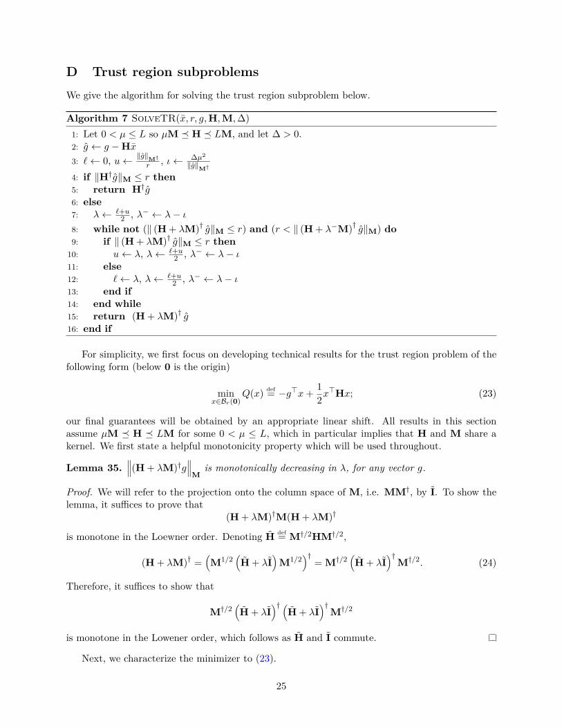
D Trust region subproblemsWe give the algorithm for solving the trust region subproblem below.

Algorithm 7 SolveTR(x, r, g,H,M,∆)1: Let 0 < µ ≤ L so µM H LM, and let ∆ > 0.2: g ← g −Hx

3: `← 0, u← ‖g‖M†r , ι← ∆µ2

‖g‖M†

4: if ‖H†g‖M ≤ r then5: return H†g6: else7: λ← `+u

2 , λ− ← λ− ι8: while not (‖ (H + λM)† g‖M ≤ r) and (r < ‖ (H + λ−M)† g‖M) do9: if ‖ (H + λM)† g‖M ≤ r then

10: u← λ, λ← `+u2 , λ− ← λ− ι

11: else12: `← λ, λ← `+u

2 , λ− ← λ− ι13: end if14: end while15: return (H + λM)† g16: end if

For simplicity, we first focus on developing technical results for the trust region problem of thefollowing form (below 0 is the origin)

minx∈Br(0)

Q(x) def= −g>x+ 12x>Hx; (23)

our final guarantees will be obtained by an appropriate linear shift. All results in this sectionassume µM H LM for some 0 < µ ≤ L, which in particular implies that H and M share akernel. We first state a helpful monotonicity property which will be used throughout.

Lemma 35.∥∥∥(H + λM)†g

∥∥∥M

is monotonically decreasing in λ, for any vector g.

Proof. We will refer to the projection onto the column space of M, i.e. MM†, by I. To show thelemma, it suffices to prove that

(H + λM)†M(H + λM)†

is monotone in the Loewner order. Denoting H def= M†/2HM†/2,

(H + λM)† =(M1/2

(H + λI

)M1/2

)†= M†/2

(H + λI

)†M†/2. (24)

Therefore, it suffices to show that

M†/2(H + λI

)† (H + λI

)†M†/2

is monotone in the Lowener order, which follows as H and I commute.

Next, we characterize the minimizer to (23).

25

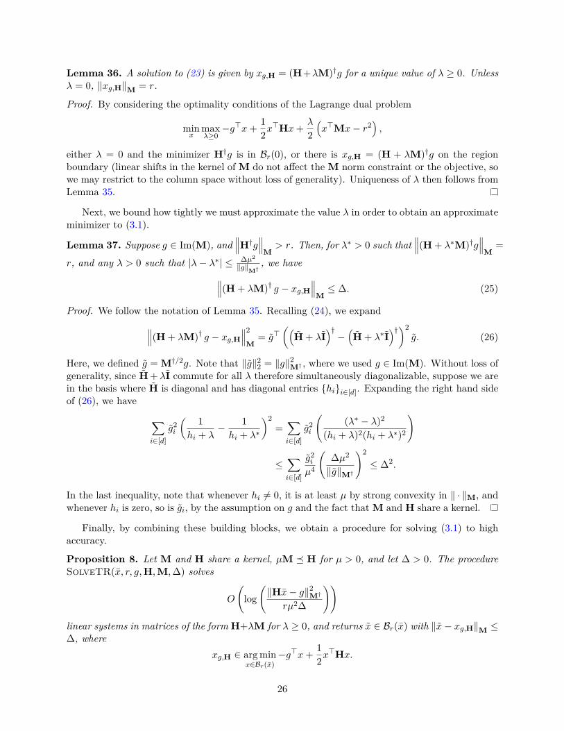
Lemma 36. A solution to (23) is given by xg,H = (H+λM)†g for a unique value of λ ≥ 0. Unlessλ = 0, ‖xg,H‖M = r.

Proof. By considering the optimality conditions of the Lagrange dual problem

minx

maxλ≥0−g>x+ 1

2x>Hx+ λ

2(x>Mx− r2

),

either λ = 0 and the minimizer H†g is in Br(0), or there is xg,H = (H + λM)†g on the regionboundary (linear shifts in the kernel of M do not affect the M norm constraint or the objective, sowe may restrict to the column space without loss of generality). Uniqueness of λ then follows fromLemma 35.

Next, we bound how tightly we must approximate the value λ in order to obtain an approximateminimizer to (3.1).

Lemma 37. Suppose g ∈ Im(M), and∥∥∥H†g∥∥∥

M> r. Then, for λ∗ > 0 such that

∥∥∥(H + λ∗M)†g∥∥∥

M=

r, and any λ > 0 such that |λ− λ∗| ≤ ∆µ2

‖g‖M†, we have∥∥∥(H + λM)† g − xg,H

∥∥∥M≤ ∆. (25)

Proof. We follow the notation of Lemma 35. Recalling (24), we expand∥∥∥(H + λM)† g − xg,H∥∥∥2

M= g>

((H + λI

)†−(H + λ∗I

)†)2g. (26)

Here, we defined g = M†/2g. Note that ‖g‖22 = ‖g‖2M† , where we used g ∈ Im(M). Without loss ofgenerality, since H + λI commute for all λ therefore simultaneously diagonalizable, suppose we arein the basis where H is diagonal and has diagonal entries hii∈[d]. Expanding the right hand sideof (26), we have

∑i∈[d]

g2i

( 1hi + λ

− 1hi + λ∗

)2=∑i∈[d]

g2i

((λ∗ − λ)2

(hi + λ)2(hi + λ∗)2

)

≤∑i∈[d]

g2i

µ4

(∆µ2

‖g‖M†

)2

≤ ∆2.

In the last inequality, note that whenever hi 6= 0, it is at least µ by strong convexity in ‖ · ‖M, andwhenever hi is zero, so is gi, by the assumption on g and the fact that M and H share a kernel.

Finally, by combining these building blocks, we obtain a procedure for solving (3.1) to highaccuracy.

Proposition 8. Let M and H share a kernel, µM H for µ > 0, and let ∆ > 0. The procedureSolveTR(x, r, g,H,M,∆) solves

O

(log

(‖Hx− g‖2M†

rµ2∆

))

linear systems in matrices of the form H+λM for λ ≥ 0, and returns x ∈ Br(x) with ‖x− xg,H‖M ≤∆, where

xg,H ∈ arg minx∈Br(x)

−g>x+ 12x>Hx.

26

Proof. First, for g def= g −Hx, we have the equivalent problem

arg min‖y‖M≤r

−g>(y + x) + 12(y + x)>H(y + x) = arg min

y∈Br(0)−g>y + 1

2y>Hy.

Following Lemma 36, in Line 4 we verify whether for the optimal solution, λ = 0, using one linearsystem solve. If not, by monotonicity of

∥∥∥(H + λM)†g∥∥∥

Min λ (Lemma 35), it is clear that the

value λ∗ corresponding to the solution lies in the range [`, u] = [0, ‖g‖M† /r], by∥∥∥∥∥(

H + ‖g‖M†r

M)†g

∥∥∥∥∥2

M≤ r2.

This follows from e.g. the characterization (24). Therefore, Lemma 37 shows that it suffices toperform a binary search over this region to find a value λ with additive error ι = ∆µ2

‖g‖M†to output

a solution x of the desired accuracy. We note that we may check feasibility in Br(0) by computingthe value of

∥∥∥(H + λM)†g∥∥∥

Mdue to Lemma 36, and it suffices to output the larger value of λ

amongst the endpoint of the interval of length ι containing λ∗, reflecting our termination conditionin Line 8.

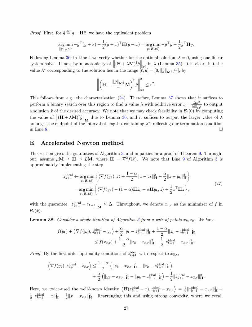
E Accelerated Newton methodThis section gives the guarantees of Algorithm 3, and in particular a proof of Theorem 9. Through-out, assume µM H LM, where H = ∇2f(x). We note that Line 9 of Algorithm 3 isapproximately implementing the step

zidealk+1 ← arg min

z∈Br(x)

〈∇f(yk), z〉+ 1− α

2 ‖z − zk‖2H + α

2 ‖z − yk‖2H

= arg min

z∈Br(x)

〈∇f(yk)− (1− α)Hzk − αHyk, z〉+ 1

2z>Hz

,

(27)

with the guarantee∥∥∥zidealk+1 − zk+1

∥∥∥M≤ ∆. Throughout, we denote xx,r as the minimizer of f in

Br(x).

Lemma 38. Consider a single iteration of Algorithm 3 from a pair of points xk, zk. We have

f(yk) +⟨∇f(yk), zideal

k+1 − yk⟩

+ α

2 ‖yk − zidealk+1 ‖2H + 1− α

2 ‖zk − zidealk+1 ‖2H

≤ f(xx,r) + 1− α2 ‖zk − xx,r‖2H −

12‖z

idealk+1 − xx,r‖2H.

Proof. By the first-order optimality conditions of zidealk+1 with respect to xx,r,⟨

∇f(yk), zidealk+1 − xx,r

⟩≤ 1− α

2(‖zk − xx,r‖2H − ‖zk − zideal

k+1 ‖2H)

+ α

2(‖yk − xx,r‖2H − ‖yk − zideal

k+1 ‖2H)− 1

2‖zidealk+1 − xx,r‖2H.

Here, we twice-used the well-known identity⟨H(zideal

k+1 − x), zidealk+1 − xx,r

⟩= 1

2‖zidealk+1 − xx,r‖2H +

12‖z

idealk+1 − x‖2H − 1

2‖x − xx,r‖2H. Rearranging this and using strong convexity, where we recall

27

α = c−1,

f(yk) +⟨∇f(yk), zideal

k+1 − yk⟩

+ α

2 ‖yk − zidealk+1 ‖2H + 1− α

2 ‖zk − zidealk+1 ‖2H

≤(f(yk) + 〈∇f(yk), xx,r − yk〉+ α

2 ‖yk − xx,r‖2H

)+ 1− α

2 ‖zk − xx,r‖2H −12‖z

idealk+1 − xx,r‖2H

≤ f(xx,r) + 1− α2 ‖zk − xx,r‖2H −

12‖z

idealk+1 − xx,r‖2H.

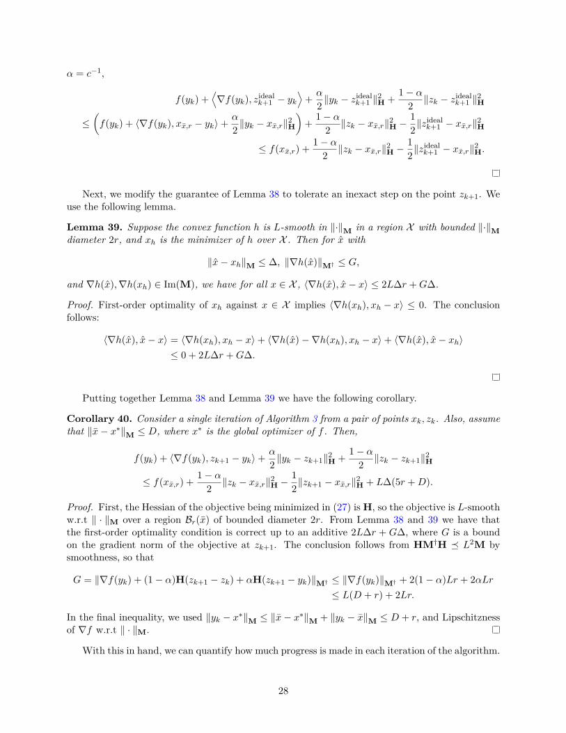
Next, we modify the guarantee of Lemma 38 to tolerate an inexact step on the point zk+1. Weuse the following lemma.

Lemma 39. Suppose the convex function h is L-smooth in ‖·‖M in a region X with bounded ‖·‖Mdiameter 2r, and xh is the minimizer of h over X . Then for x with

‖x− xh‖M ≤ ∆, ‖∇h(x)‖M† ≤ G,

and ∇h(x),∇h(xh) ∈ Im(M), we have for all x ∈ X , 〈∇h(x), x− x〉 ≤ 2L∆r +G∆.

Proof. First-order optimality of xh against x ∈ X implies 〈∇h(xh), xh − x〉 ≤ 0. The conclusionfollows:

〈∇h(x), x− x〉 = 〈∇h(xh), xh − x〉+ 〈∇h(x)−∇h(xh), xh − x〉+ 〈∇h(x), x− xh〉≤ 0 + 2L∆r +G∆.

Putting together Lemma 38 and Lemma 39 we have the following corollary.

Corollary 40. Consider a single iteration of Algorithm 3 from a pair of points xk, zk. Also, assumethat ‖x− x∗‖M ≤ D, where x∗ is the global optimizer of f . Then,

f(yk) + 〈∇f(yk), zk+1 − yk〉+ α

2 ‖yk − zk+1‖2H + 1− α2 ‖zk − zk+1‖2H

≤ f(xx,r) + 1− α2 ‖zk − xx,r‖2H −

12‖zk+1 − xx,r‖2H + L∆(5r +D).

Proof. First, the Hessian of the objective being minimized in (27) is H, so the objective is L-smoothw.r.t ‖ · ‖M over a region Br(x) of bounded diameter 2r. From Lemma 38 and 39 we have thatthe first-order optimality condition is correct up to an additive 2L∆r + G∆, where G is a boundon the gradient norm of the objective at zk+1. The conclusion follows from HM†H L2M bysmoothness, so that

G = ‖∇f(yk) + (1− α)H(zk+1 − zk) + αH(zk+1 − yk)‖M† ≤ ‖∇f(yk)‖M† + 2(1− α)Lr + 2αLr≤ L(D + r) + 2Lr.

In the final inequality, we used ‖yk − x∗‖M ≤ ‖x− x∗‖M + ‖yk − x‖M ≤ D + r, and Lipschitznessof ∇f w.r.t ‖ · ‖M.

With this in hand, we can quantify how much progress is made in each iteration of the algorithm.

28

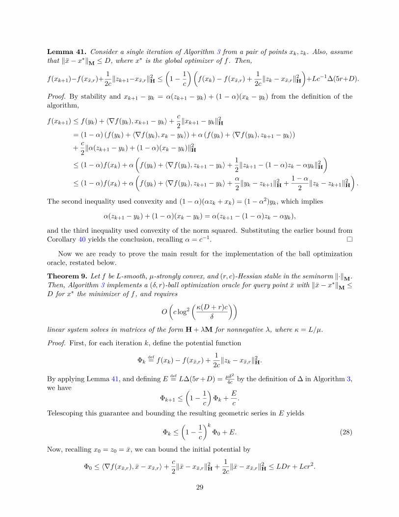
Lemma 41. Consider a single iteration of Algorithm 3 from a pair of points xk, zk. Also, assumethat ‖x− x∗‖M ≤ D, where x∗ is the global optimizer of f . Then,

f(xk+1)−f(xx,r)+12c‖zk+1−xx,r‖2H ≤

(1− 1

c

)(f(xk)− f(xx,r) + 1

2c‖zk − xx,r‖2H

)+Lc−1∆(5r+D).

Proof. By stability and xk+1 − yk = α(zk+1 − yk) + (1 − α)(xk − yk) from the definition of thealgorithm,

f(xk+1) ≤ f(yk) + 〈∇f(yk), xk+1 − yk〉+ c

2‖xk+1 − yk‖2H= (1− α) (f(yk) + 〈∇f(yk), xk − yk〉) + α (f(yk) + 〈∇f(yk), zk+1 − yk〉)

+ c

2‖α(zk+1 − yk) + (1− α)(xk − yk)‖2H

≤ (1− α)f(xk) + α

(f(yk) + 〈∇f(yk), zk+1 − yk〉+ 1

2‖zk+1 − (1− α)zk − αyk‖2H)

≤ (1− α)f(xk) + α

(f(yk) + 〈∇f(yk), zk+1 − yk〉+ α

2 ‖yk − zk+1‖2H + 1− α2 ‖zk − zk+1‖2H

).

The second inequality used convexity and (1− α)(αzk + xk) = (1− α2)yk, which implies

α(zk+1 − yk) + (1− α)(xk − yk) = α(zk+1 − (1− α)zk − αyk),

and the third inequality used convexity of the norm squared. Substituting the earlier bound fromCorollary 40 yields the conclusion, recalling α = c−1.

Now we are ready to prove the main result for the implementation of the ball optimizationoracle, restated below.

Theorem 9. Let f be L-smooth, µ-strongly convex, and (r, c)-Hessian stable in the seminorm ‖·‖M.Then, Algorithm 3 implements a (δ, r)-ball optimization oracle for query point x with ‖x− x∗‖M ≤D for x∗ the minimizer of f , and requires

O

(c log2

(κ(D + r)c

δ

))linear system solves in matrices of the form H + λM for nonnegative λ, where κ = L/µ.

Proof. First, for each iteration k, define the potential function

Φkdef= f(xk)− f(xx,r) + 1

2c‖zk − xx,r‖2H.

By applying Lemma 41, and defining E def= L∆(5r+D) = µδ2

4c by the definition of ∆ in Algorithm 3,we have

Φk+1 ≤(

1− 1c

)Φk + E

c.

Telescoping this guarantee and bounding the resulting geometric series in E yields

Φk ≤(

1− 1c

)kΦ0 + E. (28)

Now, recalling x0 = z0 = x, we can bound the initial potential by

Φ0 ≤ 〈∇f(xx,r), x− xx,r〉+ c

2‖x− xx,r‖2H + 1

2c‖x− xx,r‖2H ≤ LDr + Lcr2.

29

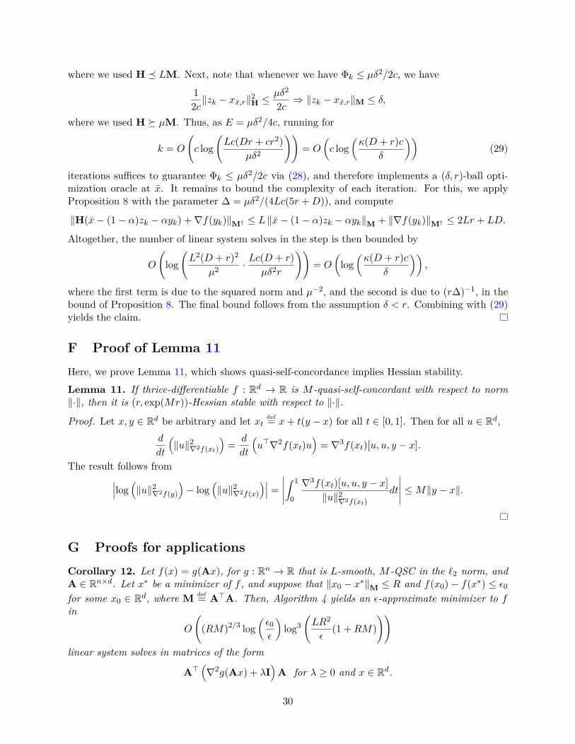
where we used H LM. Next, note that whenever we have Φk ≤ µδ2/2c, we have

12c‖zk − xx,r‖

2H ≤

µδ2

2c ⇒ ‖zk − xx,r‖M ≤ δ,

where we used H µM. Thus, as E = µδ2/4c, running for

k = O

(c log

(Lc(Dr + cr2)

µδ2

))= O

(c log

(κ(D + r)c

δ

))(29)

iterations suffices to guarantee Φk ≤ µδ2/2c via (28), and therefore implements a (δ, r)-ball opti-mization oracle at x. It remains to bound the complexity of each iteration. For this, we applyProposition 8 with the parameter ∆ = µδ2/(4Lc(5r +D)), and compute

‖H(x− (1− α)zk − αyk) +∇f(yk)‖M† ≤ L ‖x− (1− α)zk − αyk‖M + ‖∇f(yk)‖M† ≤ 2Lr + LD.

Altogether, the number of linear system solves in the step is then bounded by

O

(log

(L2(D + r)2

µ2 · Lc(D + r)µδ2r

))= O

(log

(κ(D + r)c

δ

)),

where the first term is due to the squared norm and µ−2, and the second is due to (r∆)−1, in thebound of Proposition 8. The final bound follows from the assumption δ < r. Combining with (29)yields the claim.

F Proof of Lemma 11Here, we prove Lemma 11, which shows quasi-self-concordance implies Hessian stability.

Lemma 11. If thrice-differentiable f : Rd → R is M -quasi-self-concordant with respect to norm‖·‖, then it is (r, exp(Mr))-Hessian stable with respect to ‖·‖.

Proof. Let x, y ∈ Rd be arbitrary and let xtdef= x+ t(y − x) for all t ∈ [0, 1]. Then for all u ∈ Rd,

d

dt

(‖u‖2∇2f(xt)

)= d

dt

(u>∇2f(xt)u

)= ∇3f(xt)[u, u, y − x].

The result follows from∣∣∣log(‖u‖2∇2f(y)

)− log

(‖u‖2∇2f(x)

)∣∣∣ =∣∣∣∣∣∫ 1

0

∇3f(xt)[u, u, y − x]‖u‖2∇2f(xt)

dt

∣∣∣∣∣ ≤M‖y − x‖.

G Proofs for applicationsCorollary 12. Let f(x) = g(Ax), for g : Rn → R that is L-smooth, M -QSC in the `2 norm, andA ∈ Rn×d. Let x∗ be a minimizer of f , and suppose that ‖x0 − x∗‖M ≤ R and f(x0)− f(x∗) ≤ ε0for some x0 ∈ Rd, where M def= A>A. Then, Algorithm 4 yields an ε-approximate minimizer to fin

O

((RM)2/3 log

(ε0ε

)log3

(LR2

ε(1 +RM)

))linear system solves in matrices of the form

A>(∇2g(Ax) + λI

)A for λ ≥ 0 and x ∈ Rd.

30

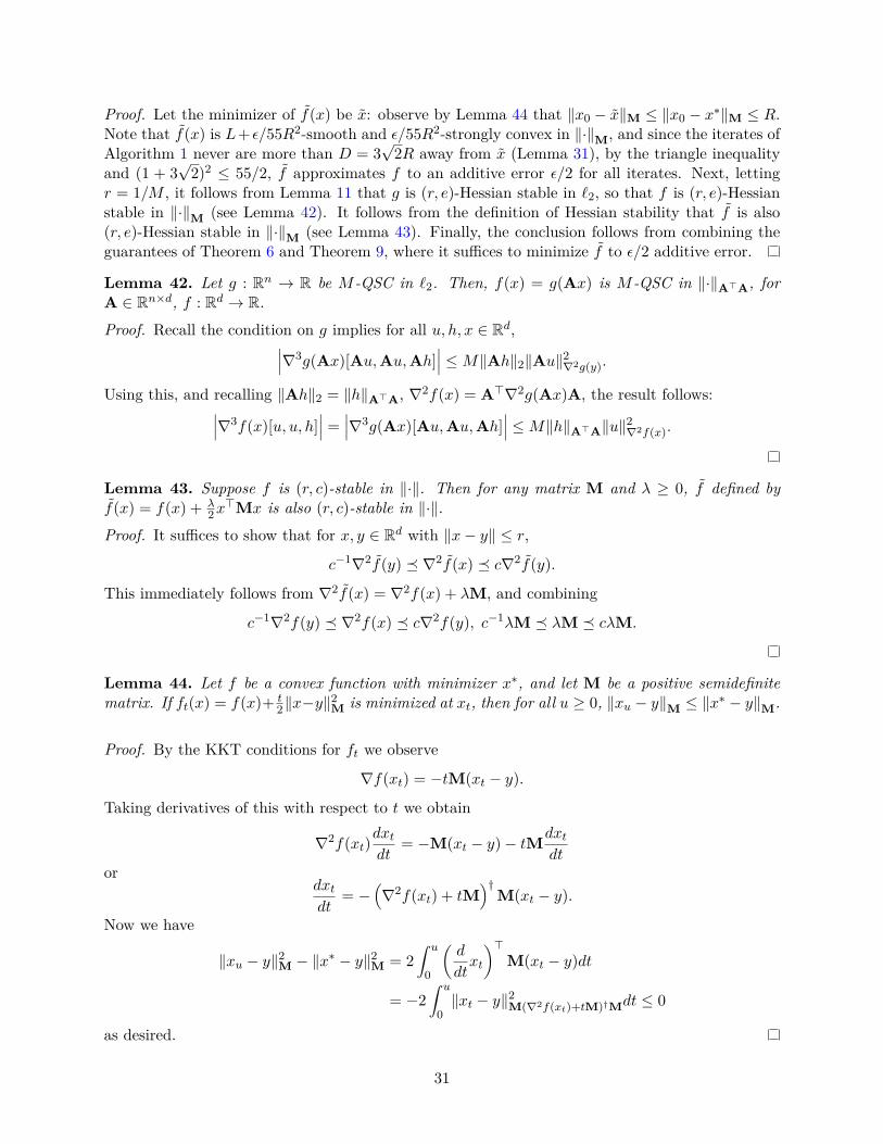
Proof. Let the minimizer of f(x) be x: observe by Lemma 44 that ‖x0 − x‖M ≤ ‖x0 − x∗‖M ≤ R.Note that f(x) is L+ ε/55R2-smooth and ε/55R2-strongly convex in ‖·‖M, and since the iterates ofAlgorithm 1 never are more than D = 3

√2R away from x (Lemma 31), by the triangle inequality

and (1 + 3√

2)2 ≤ 55/2, f approximates f to an additive error ε/2 for all iterates. Next, lettingr = 1/M , it follows from Lemma 11 that g is (r, e)-Hessian stable in `2, so that f is (r, e)-Hessianstable in ‖·‖M (see Lemma 42). It follows from the definition of Hessian stability that f is also(r, e)-Hessian stable in ‖·‖M (see Lemma 43). Finally, the conclusion follows from combining theguarantees of Theorem 6 and Theorem 9, where it suffices to minimize f to ε/2 additive error.

Lemma 42. Let g : Rn → R be M -QSC in `2. Then, f(x) = g(Ax) is M -QSC in ‖·‖A>A, forA ∈ Rn×d, f : Rd → R.

Proof. Recall the condition on g implies for all u, h, x ∈ Rd,∣∣∣∇3g(Ax)[Au,Au,Ah]∣∣∣ ≤M‖Ah‖2‖Au‖2∇2g(y).

Using this, and recalling ‖Ah‖2 = ‖h‖A>A, ∇2f(x) = A>∇2g(Ax)A, the result follows:∣∣∣∇3f(x)[u, u, h]∣∣∣ =

∣∣∣∇3g(Ax)[Au,Au,Ah]∣∣∣ ≤M‖h‖A>A‖u‖2∇2f(x).

Lemma 43. Suppose f is (r, c)-stable in ‖·‖. Then for any matrix M and λ ≥ 0, f defined byf(x) = f(x) + λ

2x>Mx is also (r, c)-stable in ‖·‖.

Proof. It suffices to show that for x, y ∈ Rd with ‖x− y‖ ≤ r,

c−1∇2f(y) ∇2f(x) c∇2f(y).

This immediately follows from ∇2f(x) = ∇2f(x) + λM, and combining

c−1∇2f(y) ∇2f(x) c∇2f(y), c−1λM λM cλM.

Lemma 44. Let f be a convex function with minimizer x∗, and let M be a positive semidefinitematrix. If ft(x) = f(x)+ t

2‖x−y‖2M is minimized at xt, then for all u ≥ 0, ‖xu − y‖M ≤ ‖x∗ − y‖M.

Proof. By the KKT conditions for ft we observe

∇f(xt) = −tM(xt − y).

Taking derivatives of this with respect to t we obtain

∇2f(xt)dxtdt

= −M(xt − y)− tMdxtdt

ordxtdt

= −(∇2f(xt) + tM

)†M(xt − y).

Now we have

‖xu − y‖2M − ‖x∗ − y‖2M = 2∫ u

0

(d

dtxt

)>M(xt − y)dt

= −2∫ u

0‖xt − y‖2M(∇2f(xt)+tM)†Mdt ≤ 0

as desired.

31

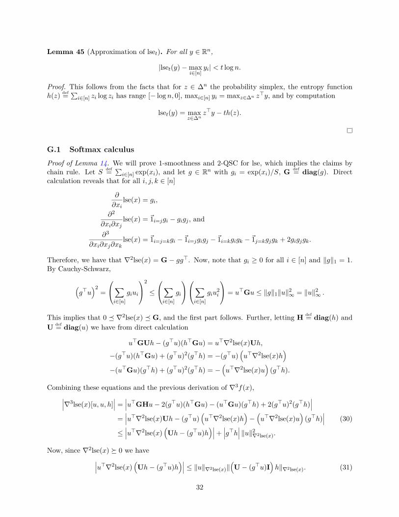
Lemma 45 (Approximation of lset). For all y ∈ Rn,

|lset(y)−maxi∈[n]

yi| < t logn.

Proof. This follows from the facts that for z ∈ ∆n the probability simplex, the entropy functionh(z) def=

∑i∈[n] zi log zi has range [− logn, 0], maxi∈[n] yi = maxz∈∆n z>y, and by computation

lset(y) = maxz∈∆n

z>y − th(z).

G.1 Softmax calculus

Proof of Lemma 14. We will prove 1-smoothness and 2-QSC for lse, which implies the claims bychain rule. Let S def=

∑i∈[n] exp(xi), and let g ∈ Rn with gi = exp(xi)/S, G def= diag(g). Direct

calculation reveals that for all i, j, k ∈ [n]

∂

∂xilse(x) = gi,

∂2

∂xi∂xjlse(x) = ~1i=jgi − gigj , and

∂3

∂xi∂xj∂xklse(x) = ~1i=j=kgi −~1i=jgigj −~1i=kgigk −~1j=kgjgk + 2gigjgk.

Therefore, we have that ∇2lse(x) = G − gg>. Now, note that gi ≥ 0 for all i ∈ [n] and ‖g‖1 = 1.By Cauchy-Schwarz,

(g>u

)2=

∑i∈[n]

giui

2

≤

∑i∈[n]

gi

∑i∈[n]

giu2i

= u>Gu ≤ ‖g‖1‖u‖2∞ = ‖u‖2∞ .

This implies that 0 ∇2lse(x) G, and the first part follows. Further, letting H def= diag(h) andU def= diag(u) we have from direct calculation

u>GUh− (g>u)(h>Gu) = u>∇2lse(x)Uh,

−(g>u)(h>Gu) + (g>u)2(g>h) = −(g>u)(u>∇2lse(x)h

)−(u>Gu)(g>h) + (g>u)2(g>h) = −

(u>∇2lse(x)u

)(g>h).

Combining these equations and the previous derivation of ∇3f(x),∣∣∣∇3lse(x)[u, u, h]∣∣∣ =

∣∣∣u>GHu− 2(g>u)(h>Gu)− (u>Gu)(g>h) + 2(g>u)2(g>h)∣∣∣

=∣∣∣u>∇2lse(x)Uh− (g>u)

(u>∇2lse(x)h

)−(u>∇2lse(x)u

)(g>h)

∣∣∣ (30)

≤∣∣∣u>∇2lse(x)

(Uh− (g>u)h

)∣∣∣+ ∣∣∣g>h∣∣∣ ‖u‖2∇2lse(x).

Now, since ∇2lse(x) 0 we have∣∣∣u>∇2lse(x)(Uh− (g>u)h

)∣∣∣ ≤ ‖u‖∇2lse(x)‖(U− (g>u)I

)h‖∇2lse(x). (31)

32

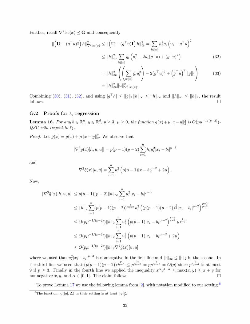
Further, recall ∇2lse(x) G and consequently

‖(U− (g>u)I

)h‖2∇2lse(x) ≤ ‖

(U− (g>u)I

)h‖2G =

∑i∈[n]

h2i gi(ui − g>u

)2

≤ ‖h‖2∞∑i∈[n]

gi(u2i − 2ui(g>u) + (g>u)2

)(32)

= ‖h‖2∞

∑i∈[n]

giu2i

− 2(g>u)2 +(g>u

)2‖g‖1

(33)

= ‖h‖2∞‖u‖2∇2lse(x).

Combining (30), (31), (32), and using |g>h| ≤ ‖g‖1‖h‖∞ ≤ ‖h‖∞ and ‖h‖∞ ≤ ‖h‖2, the resultfollows.

G.2 Proofs for `p regression

Lemma 16. For any b ∈ Rn, y ∈ Rd, p ≥ 3, µ ≥ 0, the function g(x)+µ‖x−y‖22 is O(pµ−1/(p−2))-QSC with respect to `2.

Proof. Let g(x) = g(x) + µ‖x− y‖22. We observe that

|∇3g(x)[h, u, u]| = p(p− 1)(p− 2)n∑i=1

hiu2i |xi − bi|

p−3

and∇2g(x)[u, u] =

n∑i=1

u2i

(p(p− 1)|x− b|p−2

i + 2µ).

Now,

|∇3g(x)[h, u, u]| ≤ p(p− 1)(p− 2)‖h‖∞n∑i=1

u2i |xi − bi|

p−3

≤ ‖h‖2n∑i=1

(p(p− 1)(p− 2))p

3p−6u2i

((p(p− 1)(p− 2))

23 |xi − bi|p−2

) p−3p−2

≤ O(pµ−1/(p−2))‖h‖2n∑i=1

u2i

(p(p− 1)|xi − bi|p−2

) p−3p−2 µ

1p−2

≤ O(pµ−1/(p−2))‖h‖2n∑i=1

u2i

(p(p− 1)|xi − bi|p−2 + 2µ

)≤ O(pµ−1/(p−2))‖h‖2∇2g(x)[u, u]

where we used that u2i |xi − bi|

p−3 is nonnegative in the first line and ‖·‖∞ ≤ ‖·‖2 in the second. Inthe third line we used that (p(p − 1)(p − 2))

p3p−6 ≤ p

3p3p−6 = pp

63p−6 = O(p) since p

63p−6 is at most

9 if p ≥ 3. Finally in the fourth line we applied the inequality xαy1−α ≤ max(x, y) ≤ x + y fornonnegative x, y, and α ∈ [0, 1]. The claim follows.

To prove Lemma 17 we use the following lemma from [2], with notation modified to our setting.6

6The function γp(|y|,∆) in their setting is at least ‖y‖pp.

33

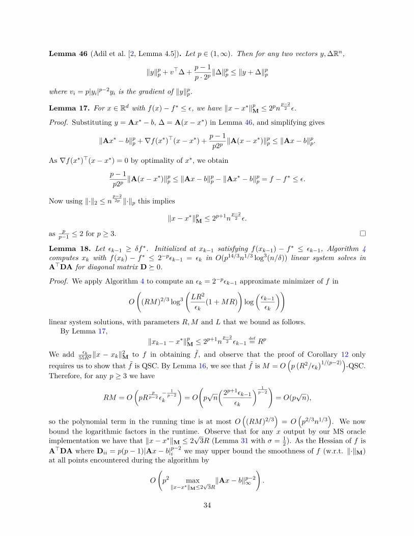
Lemma 46 (Adil et al. [2, Lemma 4.5]). Let p ∈ (1,∞). Then for any two vectors y,∆Rn,

‖y‖pp + v>∆ + p− 1p · 2p ‖∆‖

pp ≤ ‖y + ∆‖pp

where vi = p|yi|p−2yi is the gradient of ‖y‖pp.

Lemma 17. For x ∈ Rd with f(x)− f∗ ≤ ε, we have ‖x− x∗‖pM ≤ 2pnp−2

2 ε.

Proof. Substituting y = Ax∗ − b, ∆ = A(x− x∗) in Lemma 46, and simplifying gives

‖Ax∗ − b‖pp +∇f(x∗)>(x− x∗) + p− 1p2p ‖A(x− x∗)‖pp ≤ ‖Ax− b‖pp.

As ∇f(x∗)>(x− x∗) = 0 by optimality of x∗, we obtain

p− 1p2p ‖A(x− x∗)‖pp ≤ ‖Ax− b‖pp − ‖Ax∗ − b‖pp = f − f∗ ≤ ε.

Now using ‖·‖2 ≤ np−22p ‖·‖p this implies

‖x− x∗‖pM ≤ 2p+1np−2

2 ε.

as pp−1 ≤ 2 for p ≥ 3.

Lemma 18. Let εk−1 ≥ δf∗. Initialized at xk−1 satisfying f(xk−1) − f∗ ≤ εk−1, Algorithm 4computes xk with f(xk) − f∗ ≤ 2−pεk−1 = εk in O(p14/3n1/3 log3(n/δ)) linear system solves inA>DA for diagonal matrix D 0.

Proof. We apply Algorithm 4 to compute an εk = 2−pεk−1 approximate minimizer of f in

O

((RM)2/3 log3

(LR2

εk(1 +MR)

)log

(εk−1εk

))

linear system solutions, with parameters R,M and L that we bound as follows.By Lemma 17,

‖xk−1 − x∗‖pM ≤ 2p+1np−2

2 εk−1def= Rp

We add εk55R2 ‖x − xk‖2M to f in obtaining f , and observe that the proof of Corollary 12 only

requires us to show that f is QSC. By Lemma 16, we see that f is M = O(p(R2/εk

)1/(p−2))-QSC.Therefore, for any p ≥ 3 we have

RM = O

(pR

pp−2 ε

− 1p−2

k

)= O

(p√n

(2p+1εk−1εk

) 1p−2)

= O(p√n),

so the polynomial term in the running time is at most O((RM)2/3

)= O

(p2/3n1/3

). We now

bound the logarithmic factors in the runtime. Observe that for any x output by our MS oracleimplementation we have that ‖x− x∗‖M ≤ 2

√3R (Lemma 31 with σ = 1

2). As the Hessian of f isA>DA where Dii = p(p− 1)|Ax− b|p−2

i we may upper bound the smoothness of f (w.r.t. ‖·‖M)at all points encountered during the algorithm by

O

(p2 max‖x−x∗‖M≤2

√3R‖Ax− b‖p−2

∞

).

34

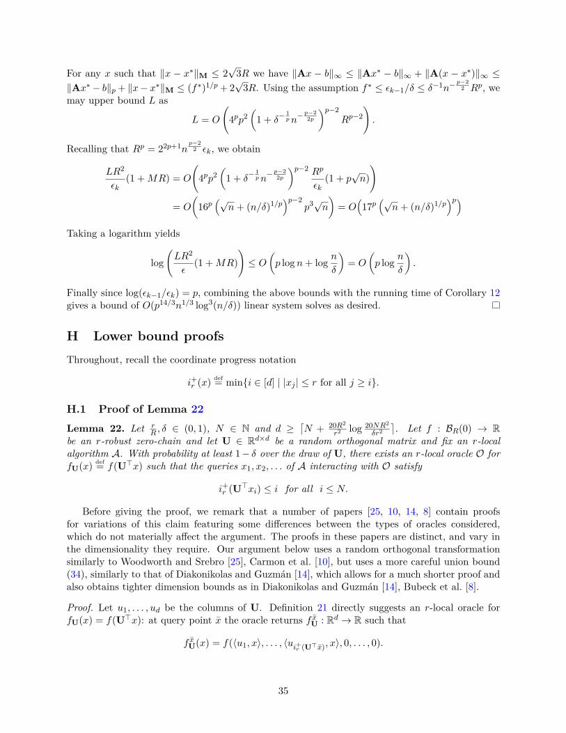
For any x such that ‖x − x∗‖M ≤ 2√

3R we have ‖Ax − b‖∞ ≤ ‖Ax∗ − b‖∞ + ‖A(x − x∗)‖∞ ≤‖Ax∗− b‖p + ‖x− x∗‖M ≤ (f∗)1/p + 2

√3R. Using the assumption f∗ ≤ εk−1/δ ≤ δ−1n−

p−22 Rp, we

may upper bound L as

L = O

(4pp2

(1 + δ

− 1pn− p−2

2p

)p−2Rp−2

).

Recalling that Rp = 22p+1np−2

2 εk, we obtain

LR2

εk(1 +MR) = O

(4pp2

(1 + δ

− 1pn− p−2

2p

)p−2 Rp

εk(1 + p

√n))

= O

(16p

(√n+ (n/δ)1/p

)p−2p3√n

)= O

(17p

(√n+ (n/δ)1/p

)p)Taking a logarithm yields

log(LR2

ε(1 +MR)

)≤ O

(p logn+ log n

δ

)= O

(p log n

δ

).

Finally since log(εk−1/εk) = p, combining the above bounds with the running time of Corollary 12gives a bound of O(p14/3n1/3 log3(n/δ)) linear system solves as desired.

H Lower bound proofsThroughout, recall the coordinate progress notation

i+r (x) def= mini ∈ [d] | |xj | ≤ r for all j ≥ i.

H.1 Proof of Lemma 22

Lemma 22. Let rR , δ ∈ (0, 1), N ∈ N and d ≥

⌈N + 20R2

r2 log 20NR2

δr2⌉. Let f : BR(0) → R

be an r-robust zero-chain and let U ∈ Rd×d be a random orthogonal matrix and fix an r-localalgorithm A. With probability at least 1− δ over the draw of U, there exists an r-local oracle O forfU(x) def= f(U>x) such that the queries x1, x2, . . . of A interacting with O satisfy

i+r (U>xi) ≤ i for all i ≤ N.

Before giving the proof, we remark that a number of papers [25, 10, 14, 8] contain proofsfor variations of this claim featuring some differences between the types of oracles considered,which do not materially affect the argument. The proofs in these papers are distinct, and vary inthe dimensionality they require. Our argument below uses a random orthogonal transformationsimilarly to Woodworth and Srebro [25], Carmon et al. [10], but uses a more careful union bound(34), similarly to that of Diakonikolas and Guzmán [14], which allows for a much shorter proof andalso obtains tighter dimension bounds as in Diakonikolas and Guzmán [14], Bubeck et al. [8].

Proof. Let u1, . . . , ud be the columns of U. Definition 21 directly suggests an r-local oracle forfU(x) = f(U>x): at query point x the oracle returns f xU : Rd → R such that

f xU(x) = f(〈u1, x〉, . . . , 〈ui+r (U>x), x〉, 0, . . . , 0).

35

The r-robust zero-chain definition implies that O(x) = f xU is a valid response for an r-local oraclefor fU. Moreover, the oracle answer to query xi only depends on the first i+r (U>xi) columns of u.Define

pidef= max

j≤ii+r

(U>xj

)to be the highest progress attained up to query i. With this notation, we wish to show that

P( ⋂i≤Npi ≤ i

)≥ 1− δ.

Note that at round i + 1 the algorithm could query xi+1 = R · upi which would satisfy pi+1 =i+r (U>xi+1) = 1 + pi. Therefore, it is possible to choose queries so that i+r (U>xi) = pi = i.However, any faster increase in pi is highly unlikely, because it would require attaining high innerproduct with a direction uj for j > pi about which we have very little information when d issufficiently large.

To make this intuition rigorous, we apply the union bound to the failure probability, giving

P( ⋃i≤Npi > i

)= P

( ⋃i≤Npi > i , pi−1 < i

)≤

N∑i=1

P(pi > i , pi−1 < i), (34)

with p0 = 0. We further upper bound each summand as

P(pi > i, pi−1 < i) = P(⋃j≥i

|〈uj , xi〉| > r , pi−1 < i

)≤ (d− i+ 1) · P

(|〈ui, xi〉| > r , pi−1 < i

),

(35)where the last step uses a union bound and the exchangeablility of ui, ui+1, . . . , ud under the eventpi−1 < i. Note that the event pi−1 < i implies that that xi depends on U only through U(<i) def=u1, . . . , ui−1, as these vectors allow us to compute the oracle responses to queries x1, . . . , xi−1.7Formally, we may write

xi = ai(U(<i))1pi−1 < i+ ai(U)1pi−1 ≥ i,

for two measurable functions ai : Rd×(i−1) → Rd and ai : Rd×d → Rd. Consequently, we have

P(|〈ui, xi〉| > r , pi−1 < i

)= P

(|〈ui, ai(U(<i))〉| > r , pi−1 < i

)≤ P

(|〈ui, ai(U(<i))〉| > r

).

Conditional on U(<i), the vector ui is uniformly distributed in the (d − i + 1)-dimensional spacespanui, . . . , ud. Therefore, standard concentration inequalities on the sphere [see 6, Lecture 8]give

P(|〈ui, ai(U(<i))〉| > r

∣∣U(<i)) ≤ 2 exp− r2

2‖ai(U(<i))‖2· (d− i+ 1)

≤ δ

d2 ,

where in the final step we substituted ‖ai(U(<i))‖ ≤ R, and our setting of d, which implies

d− i+ 1 ≥ d−N ≥ 20R2

r2 log 20NR2

δ · r2 ≥ 2R2

r2 log 2d2

δ.

Substituting P(|〈ui, xi〉| > r , pi−1 < i) ≤ δd2 into the bounds (34) and (35) concludes the proof.

7Applying Yao’s minimax principle [26] we implicitly condition our proof on the random coin tosses of A, whichis tantamount to assuming without loss of generality that A is deterministic.

36

H.2 Proof of Lemma 23

Lemma 23. Let r > 0 and N ∈ N. Define

fN,r(x) def= maxi∈[N ]xi − 4r · i (10)

1. The function fN,r is an r-robust zero-chain.

2. For all x ∈ BR(0) such that i+r (x) ≤ N , we have fN,r(x)− infz∈BR(0) fN,r(z) ≥ R√N− 4Nr.

3. The function fN,r is convex and 1-Lipschitz.

Proof. To prove the first part, fix x, x ∈ Br(x) and j > i+r (x). We have for all x ∈ Br(x) that|xk − xk| ≤ r for all k ∈ [d], and therefore

xj − 4r · j(i)≤ xj + r − 4r · j

(ii)≤ xi+r (x) + 3r − 4r · j

(iii)≤ xi+r (x) + 4r − 4r · j

(iv)≤ xi+r (x) − 4r · i+r (x).

Transitions (i) and (iii) above are due to ‖x− x‖ ≤ r; transition (ii) is due to the definition (9) ofi+r , which implies |xi+r (x)| ≤ r and |xj | ≤ r; and (iv) is due to j > i+r (x). Consequently, we have

fN,r(x) = maxi∈[i+r (x)]

xi − 4r · i for all x ∈ Br(x).

Similarly, we can use |xi+r (x)| ≤ r and j > i+r (x) to conclude that

0− 4r · j ≤ xi+r (x) + r − 4r · j ≤ xi+r (x) − 4r · i+r (x),

which means that fN,r(x) = maxi∈[i+r (x)]xi−4r ·i = fN,r(x1, . . . , xi+r (x), 0, . . . , 0), giving the robustzero-chain property.

The second property is well-known [see, e.g., 8], but we show it here for completeness. Considerthe point x = − R√

N1 ∈ BR(0). Clearly, infz∈BR(0) fN,r(z) ≤ fN,r(x) = − R√

N− 4r. Moreover, for

any x with i+r (x) ≤ N we have fN,r(x) ≥ xN − 4Nr ≥ −(4N + 1)r. Combining these two boundsyields fN,r(x)− infz∈BR(0) fN,r(z) ≥ R√

N− (4N − 3)r ≥ R√

N− 4Nr as required.

The final property follows from the fact that maximization preserves convexity and Lipschitzconstants.

37