Absorption - graphics.stanford.edu
15
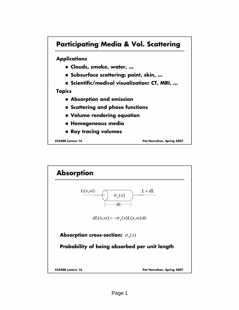
Page 1 Participating Media & Vol. Scattering Applications Clouds, smoke, water, … Subsurface scattering: paint, skin, … Scientific/medical visualization: CT, MRI, … Topics Absorption and emission Scattering and phase functions CS348B Lecture 16 Pat Hanrahan, Spring 2007 Scattering and phase functions Volume rendering equation Homogeneous media Ray tracing volumes Absorption L dL + (, ) Lx ω () a x σ ds (, ) ()(, ) a dL x xLx ds ω σ ω = − Absorption cross-section: () a x σ CS348B Lecture 16 Pat Hanrahan, Spring 2007 Probability of being absorbed per unit length a
Transcript of Absorption - graphics.stanford.edu
Page 1
Participating Media & Vol. Scattering
Applications
Clouds, smoke, water, …
Subsurface scattering: paint, skin, …
Scientific/medical visualization: CT, MRI, …
Topics
Absorption and emission
Scattering and phase functions
CS348B Lecture 16 Pat Hanrahan, Spring 2007
Scattering and phase functions
Volume rendering equation
Homogeneous media
Ray tracing volumes
Absorption
L dL+( , )L x ω( )a xσ
ds
( , ) ( ) ( , )adL x x L x dsω σ ω= −
Absorption cross-section: ( )a xσ
CS348B Lecture 16 Pat Hanrahan, Spring 2007
p
Probability of being absorbed per unit length
( )a
Page 2
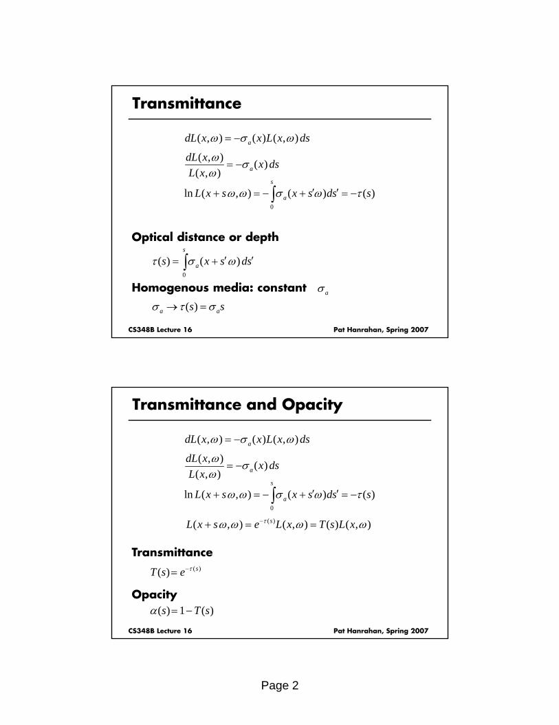
Transmittance
( , ) ( )( ) a
dL x x dsL
ω σ= −
( , ) ( ) ( , )adL x x L x dsω σ ω= −
0
ln ( , ) ( ) ( )s
aL x s x s ds sω ω σ ω τ′ ′+ = − + = −∫
s
∫
Optical distance or depth
( )( , ) aL x ω
CS348B Lecture 16 Pat Hanrahan, Spring 2007
0
( ) ( )as x s dsτ σ ω′ ′= +∫Homogenous media: constant
( )a as sσ τ σ→ =aσ
Transmittance and Opacity
( , ) ( )( ) a
dL x x dsL
ω σ= −
( , ) ( ) ( , )adL x x L x dsω σ ω= −
0
ln ( , ) ( ) ( )s
aL x s x s ds sω ω σ ω τ′ ′+ = − + = −∫
Transmittance
( )( , ) aL x ω
( )( , ) ( , ) ( ) ( , )sL x s e L x T s L xτω ω ω ω−+ = =
CS348B Lecture 16 Pat Hanrahan, Spring 2007
Transmittance( )( ) sT s e τ−=
Opacity( ) 1 ( )s T sα = −
Page 3
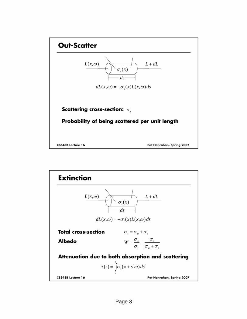
Out-Scatter
L dL+( , )L x ω( )s xσ
ds
( , ) ( ) ( , )sdL x x L x dsω σ ω= −
sσScattering cross-section:
CS348B Lecture 16 Pat Hanrahan, Spring 2007
sg
Probability of being scattered per unit length
Extinction
L dL+( , )L x ω( )t xσ
ds
( , ) ( ) ( , )tdL x x L x dsω σ ω= −
t a sσ σ σ= +Total cross-section
s sW σ σ= =Albedo
CS348B Lecture 16 Pat Hanrahan, Spring 2007
0
( ) ( )s
ts x s dsτ σ ω′ ′= +∫
Attenuation due to both absorption and scattering
t a sσ σ σ+
Page 4
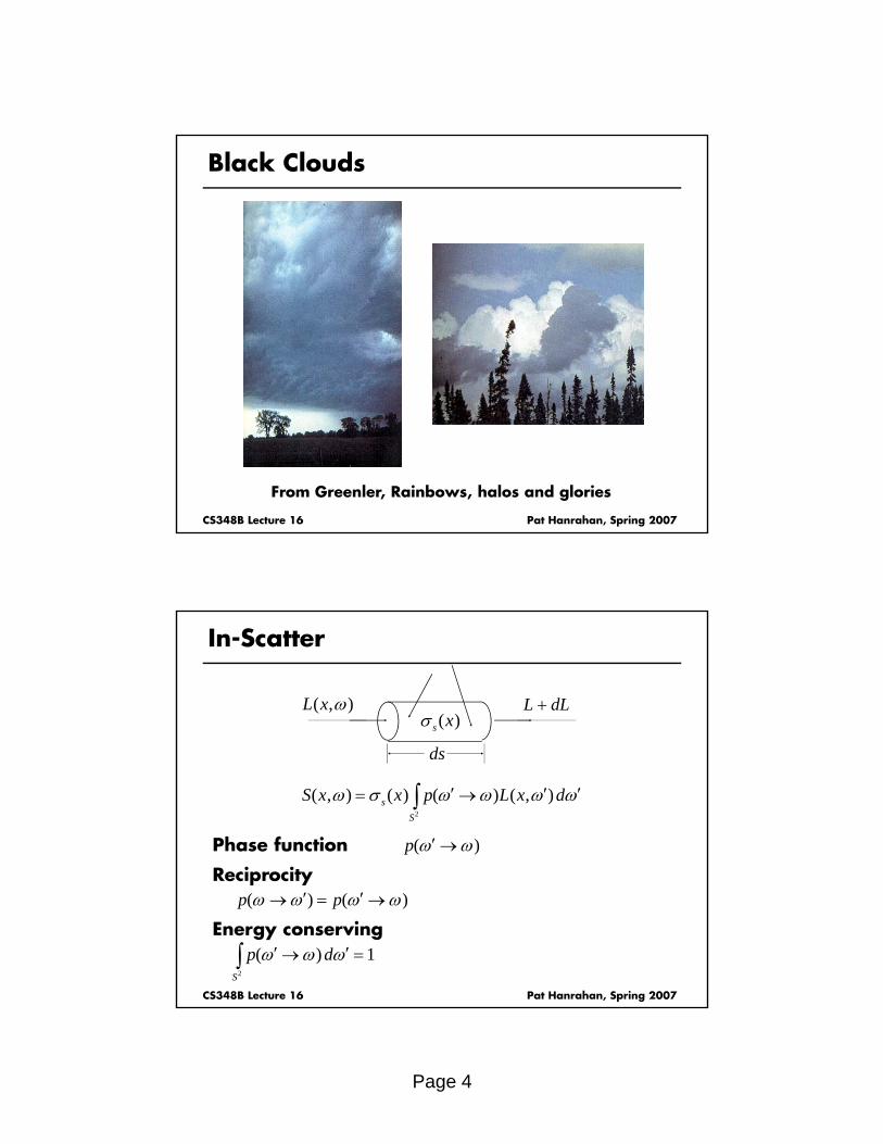
Black Clouds
CS348B Lecture 16 Pat Hanrahan, Spring 2007
From Greenler, Rainbows, halos and glories
In-Scatter
L dL+( , )L x ω( )s xσ
2
( , ) ( ) ( ) ( , )sS
S x x p L x dω σ ω ω ω ω′ ′ ′= →∫
ds
Reciprocity
Phase function ( )p ω ω′→
CS348B Lecture 16 Pat Hanrahan, Spring 2007
( ) ( )p pω ω ω ω′ ′→ = →Reciprocity
2
( ) 1S
p dω ω ω′ ′→ =∫Energy conserving
Page 5
Phase Functions
Phase angle
Phase functions
cosθ ω ω′= •
θ
ω′
ωPhase functions
(from the phase of the moon)
1. Isotropic
-simple
2. Rayleigh
1(cos )4
p θπ
=
2
4
3 1 cos(cos )p θθ +=
CS348B Lecture 16 Pat Hanrahan, Spring 2007
-molecules
3. Mie scattering
- small spheres
... Huge literature ...
4(cos )4
p θλ
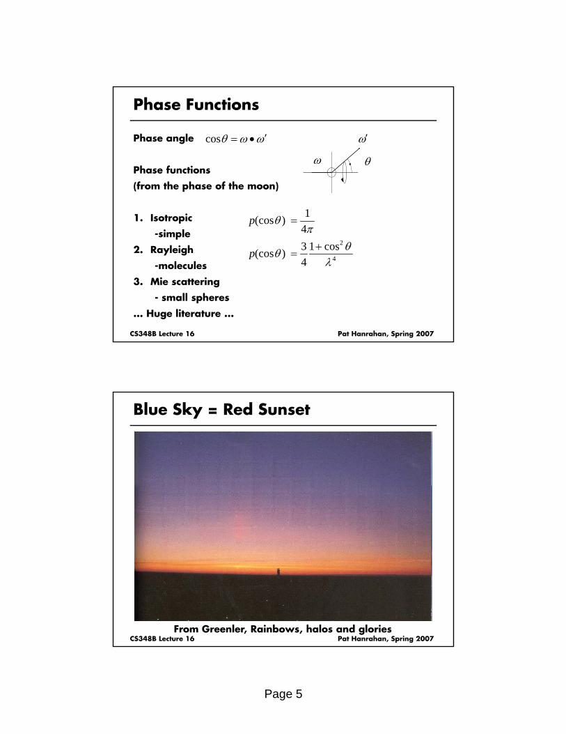
Blue Sky = Red Sunset
CS348B Lecture 16 Pat Hanrahan, Spring 2007From Greenler, Rainbows, halos and glories
Page 6
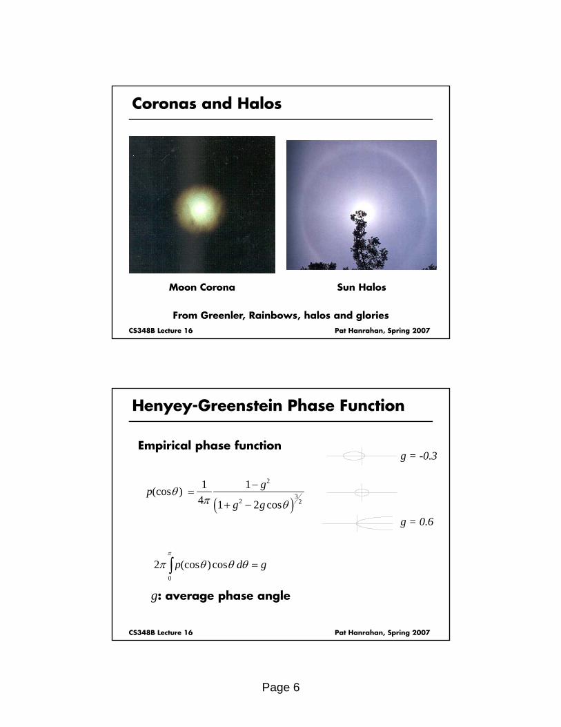
Coronas and Halos
CS348B Lecture 16 Pat Hanrahan, Spring 2007
Moon Corona Sun Halos
From Greenler, Rainbows, halos and glories
Henyey-Greenstein Phase Function
Empirical phase functiong = -0.3
( )2
32 2
1 1(cos )4 1 2 cos
gpg g
θπ θ
−=
+ −
π
g = 0.6
CS348B Lecture 16 Pat Hanrahan, Spring 2007
0
2 (cos )cosp d gπ θ θ θ =∫
g: average phase angle
Page 7
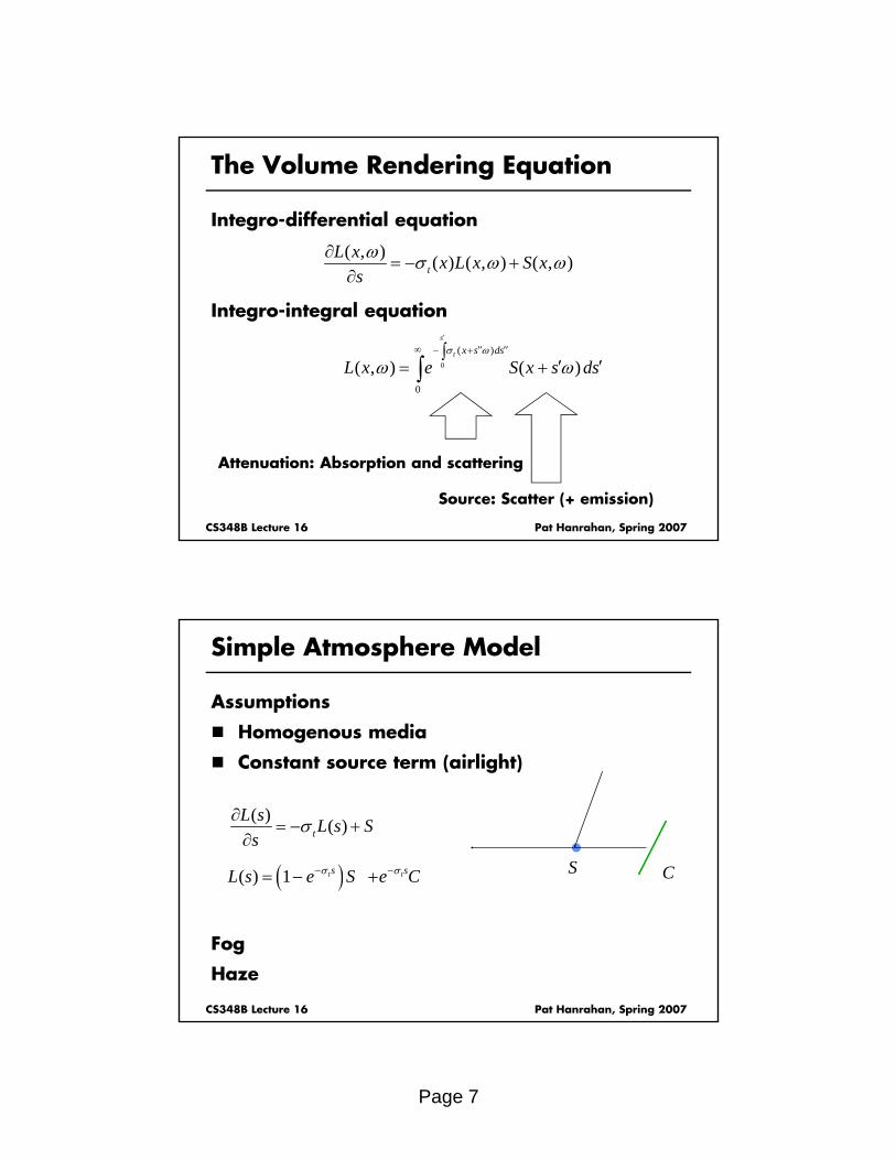
The Volume Rendering Equation
Integro-differential equation
( , ) ( ) ( , ) ( , )tL x x L x S xω σ ω ω∂
= − +∂
Integro-integral equation
( ) ( , ) ( , )ts∂
0
( )
0
( , ) ( )
s
t x s ds
L x e S x s dsσ ω
ω ω
′
∞ ′′ ′′− +∫′ ′= +∫
CS348B Lecture 16 Pat Hanrahan, Spring 2007
Attenuation: Absorption and scattering
Source: Scatter (+ emission)
Simple Atmosphere Model
Assumptions
Homogenous media
Constant source term (airlight)
( ) ( )tL s L s S
sσ∂
= − +∂
( )( ) 1 t ts sL s e S e Cσ σ− −= − + S C
CS348B Lecture 16 Pat Hanrahan, Spring 2007
Fog
Haze
( )
Page 8
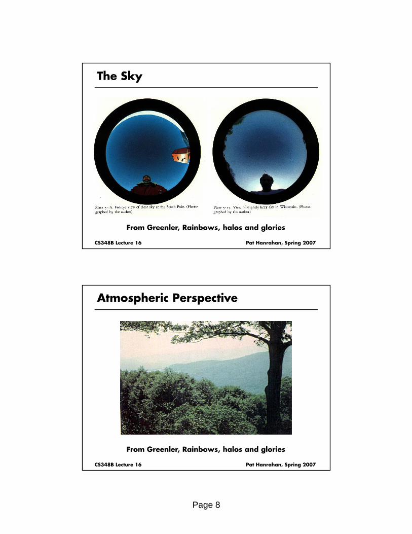
The Sky
CS348B Lecture 16 Pat Hanrahan, Spring 2007
From Greenler, Rainbows, halos and glories
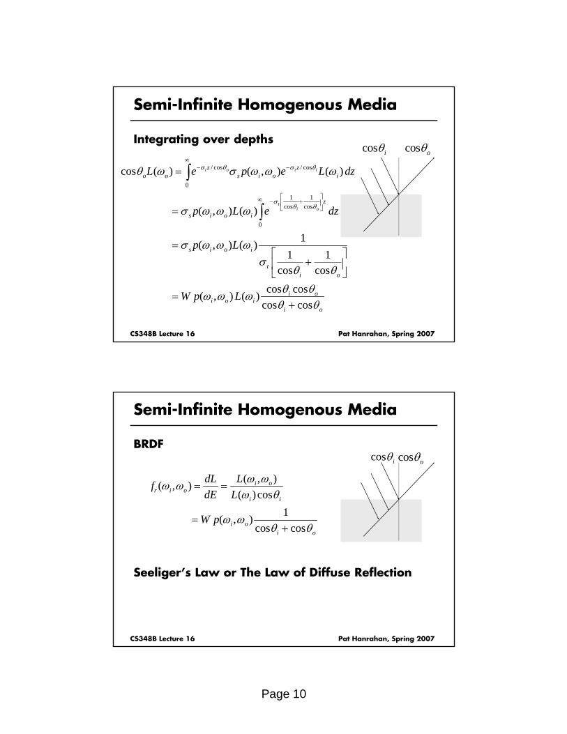
Atmospheric Perspective
CS348B Lecture 16 Pat Hanrahan, Spring 2007
From Greenler, Rainbows, halos and glories

Page 9
Atmospheric Perspective
Aerial Perspective: loss of contrast and change in color
CS348B Lecture 16 Pat Hanrahan, Spring 2007
From Musgrave
Semi-Infinite Homogenous Media
Reduced Intensity( , )( , ) (0, )iz
i iL z e Lτ ωω ω−=cos iθ cos oθ
Effective source term
Volume rendering equation
( , )cos ( , ) ( , )oo t o o
L z L z S zzωθ σ ω ω∂
= − +∂
( , )( , ) ( ) (0, )izo s i o iS z p e Lτ ωω σ ω ω ω−= →
cosz s θ=
CS348B Lecture 16 Pat Hanrahan, Spring 2007
Integrating over depths
/ cos / cos
0
cos ( ) ( , ) ( )t o t iz zo o s i o iL e p e L dzσ θ σ θθ ω σ ω ω ω
∞− −= ∫
cosdz ds θ=
Page 10
Semi-Infinite Homogenous Media
Integrating over depths
/ cos / coscos ( ) ( ) ( )t o t iz zL e p e L dzσ θ σ θθ ω σ ω ω ω∞
− −= ∫
cos iθ cos oθ
0
1 1cos cos
0
cos ( ) ( , ) ( )
( , ) ( )
1( , ) ( )1 1
ti o
o o s i o i
z
s i o i
s i o i
L e p e L dz
p L e dz
p L
σθ θ
θ ω σ ω ω ω
σ ω ω ω
σ ω ω ω
⎡ ⎤∞ − +⎢ ⎥⎣ ⎦
=
=
=⎡ ⎤
∫
∫
CS348B Lecture 16 Pat Hanrahan, Spring 2007
1 1cos cos
cos cos( , ) ( )cos cos
ti o
i oi o i
i o
W p L
σθ θ
θ θω ω ωθ θ
⎡ ⎤+⎢ ⎥
⎣ ⎦
=+
Semi-Infinite Homogenous Media
BRDF
( )LdL
cos iθ cos oθ
( , )( , )( )cos
1( , )cos cos
i or i o
i i
i oi o
LdLfdE L
W p
ω ωω ωω θ
ω ωθ θ
= =
=+
CS348B Lecture 16 Pat Hanrahan, Spring 2007
Seeliger’s Law or The Law of Diffuse Reflection
Page 11
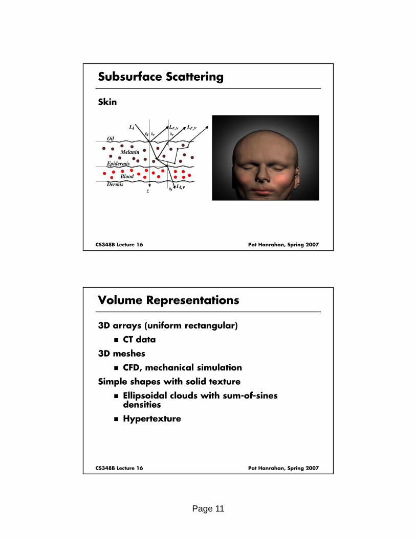
Subsurface Scattering
Skin
CS348B Lecture 16 Pat Hanrahan, Spring 2007
Volume Representations
3D arrays (uniform rectangular)
CT data
3D meshes
CFD, mechanical simulation
Simple shapes with solid texture
Ellipsoidal clouds with sum-of-sines densities
CS348B Lecture 16 Pat Hanrahan, Spring 2007
Hypertexture
Page 12
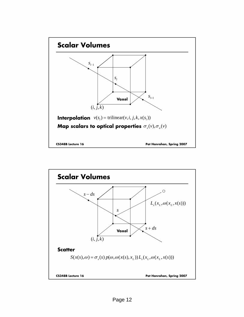
Scalar Volumes
1ls −
ls
1ls +Voxel
( , , )i j k
CS348B Lecture 16 Pat Hanrahan, Spring 2007
Interpolation
Map scalars to optical properties ( ), ( )s av vσ σ
( ) trilinear( , , , , ( ))l lv s v i j k x s=
Scalar Volumes
s ds−
( , ( , ( )))s L LL x x x sωs
s ds+Voxel
( , , )i j k
s L L
CS348B Lecture 16 Pat Hanrahan, Spring 2007
Scatter( ( ), ) ( ) ( , ( ( ), )) ( , ( , ( )))s L s L LS x s s p x s x L x x x sω σ ω ω ω=
Page 13
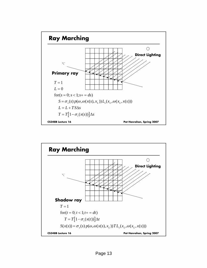
Ray Marching
Direct Lighting
Primary ray
10
f ( 0 1 )
TL
d
==
CS348B Lecture 16 Pat Hanrahan, Spring 2007
[ ]
for( 0; 1; )( ) ( , ( ( ), )) ( , ( , ( )))
1 ( ( ))
s L s L L
t
s s s dsS s p x s x L x x x sL L TS sT T x s s
σ ω ω ω
σ
= < + ==
= + Δ
= − Δ
Ray Marching
Direct Lighting
Shadow ray1T
CS348B Lecture 16 Pat Hanrahan, Spring 2007
[ ]
1for( 0; 1; )
1 ( ( ))
( ( )) ( ) ( , ( ( ), )) ( , ( , ( )))t
s L s L L
Tt t t dt
T T x t t
S x s s p x s x T L x x x s
σ
σ ω ω ω
== < + =
= − Δ
=
Page 14
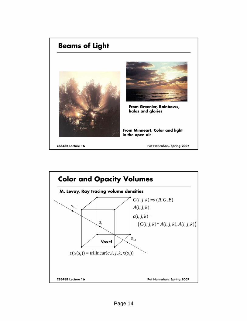
Beams of Light
From Greenler, Rainbows, halos and glories
CS348B Lecture 16 Pat Hanrahan, Spring 2007
halos and glories
From Minneart, Color and light in the open air
Color and Opacity Volumes
M. Levoy, Ray tracing volume densities
( , , ) ( , , )( , , )
C i j k R G BA i j k
⇒1ls − ( , , )A i j k1l
ls
1ls +Voxel
( )( , , )
( , , )* ( , , ), ( , , )c i j k
C i j k A i j k A i j k=
CS348B Lecture 16 Pat Hanrahan, Spring 2007
( ( )) trilinear( , , , , ( ))l lc x s c i j k x s=
Page 15
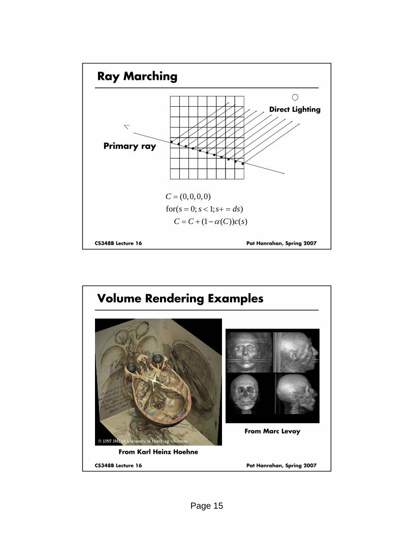
Ray Marching
Direct Lighting
Primary ray
CS348B Lecture 16 Pat Hanrahan, Spring 2007
(0,0,0,0)for( 0; 1; )
(1 ( )) ( )
Cs s s ds
C C C c sα
== < + == + −
Volume Rendering Examples
CS348B Lecture 16 Pat Hanrahan, Spring 2007
From Marc Levoy
From Karl Heinz Hoehne