Abelian varieties over finite fields

Frans OortMathematisch Instituut, P.O. Box. 80.010, NL - 3508 TA Utrecht

The Netherlandse-mail: oort@math.uu.nl

Abstract. A. Weil proved that the geometric Frobenius π = F a of anabelian variety over a finite field with q = pa elements has absolute value√

q for every embedding. T. Honda and J. Tate showed that A 7→ πA

gives a bijection between the set of isogeny classes of simple abelianvarieties over Fq and the set of conjugacy classes of q-Weil numbers.

Higher-dimensional varieties over finite fields,Summer school in Gottingen, June 2007

Introduction

We could try to classify isomorphism classes of abelian varieties. The theoryof moduli spaces of polarized abelian varieties answers this question completely.This is a geometric theory. However in this general, abstract theory it is oftennot easy to exhibit explicit examples, to construct abelian varieties with requiredproperties.

A coarser classification is that of studying isogeny classes of abelian varieties. Awonderful and powerful theorem, the Honda-Tate theory, gives

a complete classification of isogeny classes of abelian varieties over a finite field,

see Theorem 1.2.The basic idea starts with a theorem by A. Weil, a proof for the Weil conjec-

ture for an abelian variety A over a finite field K = Fq, see 3.2:

the geometric Frobenius πA of A/K is an algebraic integerwhich for every embedding ψ : Q(πA)→ C has absolute value | ψ(πA) |= √q.

For an abelian variety A over K = Fq the assignment A 7→ πA associates to A itsgeometric Frobenius πA; the isogeny class of A gives the conjugacy class of thealgebraic integer πA, and

conversely an algebraic integer which is a Weil q-numberdetermines an isogeny class, as T. Honda and J. Tate showed.

Geometric objects are constructed and classified up to isogeny by a simple alge-braic invariant. This arithmetic theory gives access to a lot of wonderful theorems.In these notes we describe this theory, we give some examples, applications andsome open questions.

Instead of reading these notes it is much better to read the wonderful and clear[73]. Some proofs have been worked out in more detail in [74].

In §§ 1 ∼ 15 material discussed in the course is described. In the appendices §§16 ∼ 22 we have gathered some information we need for statements and proofsof the main result. I hope all relevant notions and information needed for under-standing the main arguments of these notes can be found in the appendices.

Material discussed below will be contained eventually in [GM]. That book by G.van der Geer and B. Moonen can be used as a reference for all material we need,and for all results we discuss. However, as a final version of this book is not yetavailable, we also give other references. In referring to [GM] we will usually notbe precise as the final numbering can be different from the one available now.

Further recommended reading:Abelian varieties: [47], [35], [15] Chapter V.Honda-Tate theory: [73], [29], [74].Abelian varieties over finite fields: [72], [75], [77], [64].Group schemes: [62], [49].Endomorphism rings and endomorphism algebras: [68], [24], [72], [75], [54].CM-liftings: [56], [11].

Contents:§§ 1 – 13: material for this course,§§ 14, 15: examples and exercises,§§ 16 – 21: appendices giving definitions and background,§ 22: questions and open problems.

Some notation. In definitions and proofs below we need various fields, in variousdisguises. We use K, L, M, P, k, Fq, Fp = F, P, m.

We write K for an arbitrary field, usually the base field, in some cases ofarbitrary characteristic, however most of the times a finite field. We write k for analgebraically closed field. We write g for the dimension of an abelian variety, unlessotherwise stated. We write p for a prime number. We write ` for a prime number,which usually is different from the characteristic of the base field, respectivelyinvertible in the sheaf of local rings of the base scheme. We write F = Fp. We usethe notation M for a field, sometimes a field of definition for an abelian varietyin characteristic zero.

We will use L as notation for a field, usually the center of an endomorphismalgebra; we will see that in our cases this will be a totally real field or a CM-field.

We write P for a CM-field, usually of degree 2g over Q. We write P for a primefield: either P = Q or P = Fp.

A discrete valuation on a base field usually will be denoted by v, whereas adiscrete valuation on a CM-field usually will be denoted by w. If w divides p, thenormalization chosen will be given by w(p) = 1.

For a field M we denote by ΣM the set of discrete valuations (finite places) ofM . If moreover M is of characteristic zero, we denote by Σ(p)

M the set of discretevaluations with residue characteristic equal to p.

We write lim←i for the notion of “projective limit” or “inverse limit”.We write colimi→ for the notion of “inductive limit” or “direct limit”.

1. Main topic/survey

1.1. Definition. Let p be a prime number, n ∈ Z>0; write q = pn. A Weil q-numberπ is an algebraic integer such that for every embedding ψ : Q(π)→ C we have

| ψ(π) | =√q.

We say that π and π′ are conjugated if there exists an isomorphism Q(π) ∼= Q(π′)mapping π to π′.Notation: π ∼ π′.Equivalently: the minimum polynomials of π and π′ over Q are equal. We writeW (q) for the set conjugacy classes of Weil q-numbers.

In this definition | · | denotes the complex absolute value given by | a+ b√−1 |=√

a2 + b2 for a, b ∈ R. We will show that for any Weil q-number π there exists anelement π = ρ(π) ∈ Q(π) such that for any ψ : Q(π)→ C the number ψ(π) is thecomplex conjugate of ψ(π); moreover we show that π·π = q.

As Weil proved, we will see that the geometric Frobenius πA, see 3.1, of a simpleabelian variety over the finite field Fq is a Weil q-number, see Theorem 3.2. Wewill see that

A ∼ B ⇒ πA ∼ πB ,

i.e. abelian varieties defined over the same finite field K isogenous over K defineconjugated Weil numbers. We will write

simple abelian variety over K/ ∼K =: M(K, s)

for the set of isogeny classes of simple abelian varieties over K.

1.2. Theorem (Honda, Serre and Tate). Fix a finite field K = Fq. The assignmentA 7→ πA induces a bijection

simple abelian variety over K/ ∼K=M(K, s) ∼−→ W (q), A 7→ πA

from the set of K-isogeny classes of K-simple abelian varieties defined over Kand the set W (q) of conjugacy classes of Weil q-numbers.See [73].

The fact

• that the map is defined follows by Weil,• the map is injective by Tate, and• surjective by Honda and Tate.

This map will be denoted by

W :M(K, s) −→ W (q).

This theorem will be the main topic of these talks. We encounter various notionsand results, which will be exposed below (sometimes in greater generality thanstrictly necessary to understand this beautiful theorem).

1.3. Definition. We say that a Weil q-number π is effective if there exists anabelian variety A simple over Fq such that π ∼ πA. I.e. π is effective if it is in theimage of the map W : A 7→ πA/ ∼.

We indicate the steps in a proof of 1.2, which will be elaborated below. WriteK = Fq, with q = pn.

ONE (Weil) For a simple abelian variety A over a finite field K = Fq the Weilconjecture implies that πA is a Weil q-number, see Section 3, especially Theorem3.2. Hence the map

simple abelian variety over K −→ W (K), A 7→ πA

is well-defined.

TWO (Tate) For simple abelian varieties A, B defined over a finite field wehave:

A ∼ B ⇐⇒ πA ∼ πB .

See 5.3. Note that A ∼ B only makes sense if A and B are defined over thesame field. Note that πA ∼ πB implies that A and B are defined over the samefinite field. This shows that the map W : M(Fq, s) → W (q) is well-defined andinjective. See Sections 4, 5, especially Theorem 5.3.

THREE (Honda) Suppose given π ∈ W (q). There exists a finite extensionK = Fq ⊂ K ′ := FqN and an abelian variety B′ over K ′ with πN = πB′ .See [29], Theorem 1. This step says that for every Weil q-number there existsN ∈ Z>0 such that πN is effective. See Section 10 , especially Theorem 10.4.

FOUR (Tate) If π ∈ W (q) and there exists N ∈ Z>0 such that πN is effective,then π is effective. See Section 10, especially 10.5 - 10.9.

This result by Honda plus the last step shows that (A mod ∼) 7→ (πA mod ∼)is surjective.

These four steps together show that the map

W : simple abelian variety over K/ ∼K = M(K, s) ∼−→ W (q)

is bijective, thus proving the main theorem of Honda-Tate theory.

In 1966/1967 Serre wrote a letter to Tate in which he explained a proof of theManin conjecture; see Section 11. That method proved the surjectivity resultproved by Honda. Therefore, sometimes the theory discussed here can be calledthe Honda-Serre-Tate theory. As Serre’s proof was never published we can alsouse the terminology Honda-Tate theory.

We will see several examples. Here are three special cases, which we mention nowin order to convey the flavor of the aspects we will encounter.

1.4. Motivation/Some examples. See 15.5. Consider the following examples.(1) Choose q = pn, and choose i ∈ Z>0. Let π := ζi·

√q, where ζi is a primitive

i−th root of unity.(2) Choose coprime positive integers d > c > 0, and choose p. Let π be a zero of

T 2 + pcT + pd+c.

(3) Let β :=√

2 +√

3, and q = pn. Let π be a zero of

T 2 − βT + q.

In all these cases we see that π is a Weil q-number. How can we see that thesenumbers are the Weil number belonging to an isogeny class of an abelian varietysimple over Fq? Using Theorem 1.2 this follows; however these examples mightillustrate that this theorem is non-trivial. If such an isogeny class exists what isthe dimension of these abelian varieties? How can we compute this dimension?What are the p-adic properties of such an abelian variety? See 5.4, 5.5.

2. Weil numbers and CM-fields

2.1. Definition. A field L is said to be a CM-field if

• L is a finite extension of Q (i.e. L is a number field),• there is a subfield L0 ⊂ L such that L0/Q is totally real, i.e. every ψ0 :L0 → C gives ψ0(L0) ⊂ R, and

• L/L0 is quadratic totally imaginary, i.e. [L : L0] = 2 and for every ψ : L→C we have ψ(L) 6⊂ R.

Remark. The quadratic extension L/L0 gives an involution ρ ∈ Aut(L/L0). Forevery embedding ψ : L→ C this involution on a CM-field L corresponds with therestriction of complex conjugation on C to ψ(L).

2.2. Proposition. Let π be a Weil q-number.

(R) Either for at least one ψ : Q(π)→ C we have ψ(π) ∈ R; in this case we have:(Re) n is even,

√q ∈ Q, and π = +pn/2, or π = −pn/2, or

(Ro) n is odd,√q ∈ Q(

√p), and ψ(π) = ±pn/2.

In particular in case (R) we have ψ(π) ∈ R for every ψ.

(C) Or for every ψ : Q(π) → C we have ψ(π) 6∈ R (equivalently: for at least oneψ we have ψ(π) 6∈ R). In case (C) the field Q(π) is a CM-field.

See 15.9, where we explain these cases in the Honda-Tate theory.

Proof. The claims in (R) follow from the fact that ±pn/2 are precisely those realnumbers with absolute value, taken in C, are equal to

√q.

If at least one embedding ψ gives ψ(π) 6∈ R, then we are not in case (R),hence all embeddings have this property. Then

ψ(π)·ψ(π) = q.

Write β := π + qπ . Then for every ψ we have

ψ(β) = ψ(π) + (q/ψ(π)) =q

ψ(π)+ ψ(π) = ψ(β).

Hence L0 := Q(β) is totally real. For any Weil q-number π with ψ(π) 6∈ R wehave

β := π +q

π, (T − ψ(π))(T − ψ(π) ) = T 2 − βT + q ∈ Q(β)[T ].

In this case ψ(π) 6∈ R for every ψ, and L0 := Q(β) is totally real and L/L0 istotally complex. Hence L is a CM-field.

2.3. Remark. We see a characterization of Weil q-numbers:

β := π +q

πis a totally real integer,

and either π =√q ∈ R or π is a zero of

T 2 − β·T + q, with | ψ(β) |< 2√q for any ψ : Q(β)→ R.

Using this it is easy to construct Weil q-numbers, see Section 15 for some examples.

3. The Weil conjecture for abelian varieties over a finite field

3.1. The geometric Frobenius. For a scheme A→ S over a base S → Spec(Fp) incharacteristic p there is the relative Frobenius

FA/S : A −→ A(p);

see 21.2. If moreover A/S is a group scheme this is a homomorphism. If S =Spec(Fpn) there is a canonical identification A(pn) ∼=S A, and we define:

πA :=(A

FA/S−→ A(p)F

A(p)/S−→ A(p2) −→ · · · −→ A(pn) = A

).

This endomorphism is called the geometric Frobenius of A/Fpn . Sometimes wewill write (in abused notation) “ πA = Fn ”.

3.2. Theorem (Weil). Let A be a simple abelian variety over K = Fq; considerthe endomorphism πA ∈ End(A), the geometric Frobenius of A/Fq. The alge-braic number πA is a Weil q-number, i.e. it is an algebraic integer and for everyembedding ψ : Q(πA)→ C we have

| ψ(π) | =√q.

See [78], page 70; [79], page 138; [47], Theorem 4 on page 206. Using the followingtwo propositions we give a proof of this theorem.

3.3. Proposition. For any polarized abelian variety A over a field the Rosati-involution † : D → D := End0(A) is positive definite bilinear form on D, i.e. forany non-zero x ∈ D we have Tr(x·x†) > 0. See [47], Th. 1 on page 192, see [15], Th. 17.3 on page 138. For the notation Dand for the notion of the Rosati involution defined by a polarization, see Section16, in particular 16.3 and 16.5.

3.4. Proposition. For a simple abelian variety A over K = Fq we have

πA·(πA)† = q.

Here † : D → D := End0(A) is the Rosati-involution.

One proof can be found in [47], formula (i) on page 206; also see [15], Coroll. 19.2on page 144.

Another proof of 3.4 can be found in 5.21, 7.34 and Section 15 of [GM]. To thisend we study Verschiebung, see 21.3, defined for commutative flat group schemesover a base in characteristic p. The (relative) Frobenius and the Verschiebunghomomorphism for abelian varieties are related by two properties:

for any abelian variety B we have(B

F−→ B(p) V−→ B)

= p,

also V ·F = p·1B(p) , and(FB/S : B → B(p)

)t=

(VBt/S : (B(p))t → Bt

);

see 21.10. For the definition of the dual abelian scheme, and for the notation At

see 16.2. From this we see that

πAt · (πA)t =(F(At)(pn−1) · · ·FAt

) (FA(pn−1) · · ·FA

)t =

= F(At)(pn−1)

(· · ·

(F(At)(p) (FAt · VAt)V(At)(p)

)· · ·

)V(At)(pn−1) = pn = q.

In abused notation we could write: πAt · (πA)t = Fn·(Fn)t = Fn·V n = pn. 3.4

3.5. We give a proof of 3.2 using 3.4 and 3.3. We use that L = Q(πa) is the centerof D, see 5.4 (1). Hence † on D induces an involution on L. Hence † induces aninvolution †R on L ⊗Q R. This algebra is a finite product of copies of R and ofC. Using 3.3 we conclude that the involution †R is a positive definite R-linearinvolution on this product. We see that this implies that †R is the identity onevery real factor, stabilizes every complex factor, and is the complex conjugationon those factors. Conclusion:

∀x ∈ L, ∀ ψ : L→ C ⇒ ψ(x†) = ψ(x).

Hence

q = ψ(q) = ψ(πA·(πA)†

)= ψ(πA)·ψ(πA).

Hence

| ψ(πA) | =√q.

3.2

3.6. Definition/Notation. Let A be a simple abelian variety over K = Fq. Wehave seen that πA ∈ End(A) =: D. As A is simple, D is a division algebra, andQ(πA) ⊂ D is a number field (a finite extension of Q). We have seen that πA is aWeil q-number. We will say that πA is the Weil q-number attached to the simpleabelian variety A.

3.7. Simple and absolutely simple. We give an example of an abelian variety Aover a field which is K-simple, such that for some extension K ′ ⊃ K the abelianvariety A⊗K ′ is not simple, i.e. A is not absolutely simple.

Choose q = pn. Let i ∈ Z>0, and let ζ = ζi be a primitive i-th root of unity.Define π = ζ·√q. Clearly π is a Weil q-number. Using Th. 1.2, we know thereexists an abelian variety A over K, which is simple such that πA ∼ π. Assumei > 2; note that for any N which is a multiple of 2i we have Q = Q(πN ) $ Q(π).We will see: in this case g := dim(A) > 1, and A⊗ FqN ∼ (E ⊗ FqN )g where E isa supersingular curve defined over Fp. Hence in this case A is not K-simple.

3.8. Remark/Definition. We say that an abelian variety A over a fieldK is isotypicif there exists an abelian variety B simple over K and an isogeny A ∼ Bµ forsome µ ∈ Z>0; in this case we will define πA := πB ; note that fA = (fB)µ (forthe definition of fA see 16.8).

We have just seen that the property “ A is simple ” can get lost under a fieldextension. However

if A is isotypic over K and Fq = K ⊂ K ′ is an extension then A⊗K ′ is isotypic;

see 10.8.

Moreover, if K is a finite field and [K ′ : K] = N then (πA)N = πA⊗K′ ,

i.e. the formation A 7→ πA commutes under base extension with exponentiationas explained.

4. Abelian varieties with CM

4.1. smCM We say that an abelian variety X over a field K admits suffi-ciently many complex multiplications over K, abbreviated by “smCM over K”, ifEnd0(X) contains a commutative semi-simple subalgebra of rank 2·dim(X) overQ.

Equivalently: for every simple abelian variety Y over K which admits a non-zero homomorphism to X the algebra End0(Y ) contains a field of degree 2·dim(Y )over Q.

If no confusion is possible we say “A admits smCM” omitting “over K”.However we should be careful; it is possible that A, defined over K, does notadmit smCM, but that there exists a field extension K ⊂ K ′ such that A⊗K K ′

admits smCM (over K ′).

Equivalently. Suppose A ∼ ΠBi, where each of the Bi is simple. We say that Aadmits smCM, if every End0(Bi) contains a CM-subfield of degree 2·dim(Bi) overQ.

For other characterizations, see [18], page 63 and [44], page 347.

4.2. Note that if a simple abelian variety A of dimension g over a field of char-acteristic zero admits smCM then its endomorphism algebra L = End0(X) is afield, in fact a CM-field of degree 2g over Q; see 5.9. We will use he notion “CM-type” in the case of an abelian variety A over C which admits smCM, and wherethe type is given, i.e. the action of the endomorphism algebra on the tangentspace tA,0 ∼= Cg is part of the data, see 13.1. See 13.12: we do use CM-types incharacteristic zero, but we do not define (and we do not use) such a notion overfields of positive characteristic.

Note that there exist (many) abelian varieties A admitting smCM definedover a field of positive characteristic, such that End0(A) is not a field.

We could use the terminology “A has complex multiplication” to denote the caseswith End(A) % Z. However this could be misleading, and in these notes we willnot use this terminology.

It can be proved that if a simple abelian variety A admits smCM in the sensedefined above, then D = End0(A) contains a CM-field of degree 2·dim(A) overQ. Note that a field E with E ⊂ End0(A) and [E : Q] = 2·dim(A) however neednot be a CM-field; see 15.7.

Terminology. Let ϕ ∈ End0(A). Then dϕ is a K-linear endomorphism of thetangent space of A at 0 ∈ A. See 16.9. If the base field is K = C, this is justmultiplication by a complex matrix x. Suppose A(C) ∼= Cg/Λ where Λ is a latticein Cg. For ϕ ∈ End0(A) the linear map dϕ leaves Λ ⊂ Cg invariant. Converselyany complex linear map complex linear map x : Cg → Cg leaving invariant Λdefines an endomorphism ϕ of A with x = dϕ.

Consider g = 1, i.e. A is an elliptic curve and ϕ ∈ End(A). If ϕ 6∈ Z thenx ∈ C and x 6∈ R. Therefore an endomorphism of an elliptic curve over C whichis not in Z can be called “a complex multiplication”. Later this terminology wasextended to all abelian varieties.

Warning. Sometimes the terminology “an abelian variety with CM” is used, whenone wants to say “admitting smCM”; we will not adopt that confusing termi-nology. An elliptic curve E has End(E) % Z if and only if it admits smCM.However it is easy to give an abelian variety A which “admits CM”, meaningthat End(A) % Z, such that A does not admit smCM. However we will use theterminology “a CM-abelian variety” for an abelian variety which admits smCM.

It can happen that an abelian variety A over a field K does not admit smCM,and that A⊗K ′ does admit smCM.

4.3. Exercise. Show that for any elliptic curve E defined over Q we have End(E) =Z.

Show there exists an abelian surface A over Q with Z 6= End(A) = End(A⊗Q).

Show there exists an abelian variety A over a field k such that Z $ End(A)and such that A does not admit smCM.See 15.6, 18.10.

4.4. Remark. An abelian variety over a field of characteristic zero which admitssmCM is defined over a number field. See [69], Proposition 26 on page 109. Alsosee [51].

We will see that a theorem of Tate, see Theorem 5.4 implies that an abelianvariety defined over a finite field does admit smCM. By Grothendieck we knowthat an abelian variety which admits smCM up to isogeny is defined over a finitefield, see 4.5.

4.5. Remark. The converse of Tate’s result 5.4 (2) is almost true; see 5.7.

It is easy to give an example of an abelian variety, over a field of characteristicp, with smCM which is not defined over a finite field. E. g. see 5.8.

4.6. Lemma. Let K be a field, and let A be an abelian variety simple over K whichadmits smCM. Choose a CM-field P with [P : Q] = 2·dim(A) inside End0(A).(This is possible by Lemma 10.1.) Then there exists a K-isogeny A ∼K B suchthat OP → End(B), where OP is the ring of integers of P . See [80], page 308.

In [80] we also find: if A in positive characteristic admits smCM by a CM-field L,and the ring of integers OL is contained in End(A) then A can be defined over afinite field, see [80], Th. 1.3. This gives a new proof of Theorem 4.5, see [80], Th.1.4.

4.7. Definition CM-type. Let P be a CM-field of degree 2g. Let C be an al-gebraically closed field of characteristic zero. The set Hom(P,C) has 2g ele-ments. For any ϕ : P → C the homomorphism ϕ·ρ is different from ϕ. A subsetΦ ⊂ Hom(P,C) is called a CM-type for P if Hom(P,C) = Φ

∐ρ(Φ). Equivalently:

For every ϕ : P → C either ϕ ∈ Φ or ϕ·ρ ∈ Φ.

4.8. Let A be an abelian variety simple over C which admits smCM. LetP = End0(A). This is a CM-field of degree 2·dim(A). The action of P on thetangent space tA,0 splits as a direct sum of one-dimensional representations (asP is commutative and C is algebraically closed of characteristic zero). Hence thisrepresentation is given by Φ = ϕ1, · · · , ϕg. One shows this is a CM-type (i.e.these homomorphisms ϕi : P → C are mutually different and either ϕ ∈ Φ orϕ·ρ ∈ Φ). For the converse construction see 19.6.

5. Tate: The structure of End0(A): abelian varieties over finite fields.

Main references: [72], [73]. Also see the second printing of [47], especially Appendix1 by C. P. Ramanujam.

5.1. For a simple abelian variety over a field K the algebra End0(A) is a divisionalgebra. By the classification of Albert, see 18.2, we know the structure theoremof such algebras 18.4. Moreover, as Albert, Shimura and Gerritzen showed, forany algebra D in the list by Albert, and for any characteristic, there is an abelianvariety having D as endomorphism algebra. However over a finite field not alltypes do appear, there are restrictions; see 2.2, 15.9.

For an element β ∈ Q we write IrrQ(β) = Irr(β) ∈ Q[T ] for the irreducible, monicpolynomial having β as zero, the minimum polynomal of β.

5.2. Tate described properties of the endomorphism algebra of a simple abelianvariety over K = Fq, with q = pn. We write πA for the geometric Frobeniusof A, and fA = fA,πA

for the characteristic polynomial of πA. We write WriteIrrQ(πA) = Irr(πA) ∈ Z[T ] for the minimum polynomial of πA over Q. For thedefinition of a characteristic polynomial of an endomorphism, see 16.8.

The following theorems are due to Tate; these results (and much more) canbe found: [72], Theorem 1 on page 139, [72], Theorem 2 on page 140 and [73], Th.1 on page 96, [47], Appendix 1.

5.3. Theorem (Tate). Let A be an abelian variety over the finite field K = Fq.The characteristic polynomial fA,πA

= fA ∈ Z[T ] of πA ∈ End(A) is of degree2·dim(A), the constant term equals qdim(A) and fA(πA) = 0.

If an abelian variety A is K-simple then fA is a power of the minimumpolynomial Irr(πA) ∈ Z[T ].

Let A and B be abelian variety over K = Fq. Then:

A is K-isogenous to an abelian subvariety of B iff fA divides fB.

In particular

A ∼K B ⇐⇒ fA = fB .

Remark. Note that for an abelian variety A over a finite field the characteristicpolynomial fA of πA ∈ End(A) is a power of an irreducible polynomial then A isisotypic (not necessarily simple); it seems that a statement in [74] in Th. 1.1 of“The theorem of Honda and Tate” needs a small correction on this point.

For an abelian variety A over a field the endomorphism algebra End0(A) is asemi-simple ring. If moreover A is K-simple, then D = End0(A) is a division ring(hence a simple ring).

5.4. Theorem (Tate). Suppose A is a simple abelian variety over the finite fieldK = Fq.(1) The center of D := End0(A) equals L := Q(πA).(2) Moreover

2g = [L : Q]·√

[D : L],

where g is the dimension of A. Hence: every abelian variety over a finite fieldadmits smCM. See 4.1. We have:

fA = (Irr(πA))√

[D:L].

(3)

Q ⊂ L := Q(πA) ⊂ D = End0(A).

The central simple algebra D/L

• does not split at every real place of L,• does split at every finite place not above p.

• For a discrete valuation w of L with w | p the invariant of D/L is given by

invw(D/L) =w(πA)w(q)

·[Lw : Qp] mod Z,

where Lw is the local field obtained from L by completing at w. Moreover

invw(D/L) + invw(D/L) = 0 mod Z,

where w = ρ(w) is the complex conjugate of w.

5.5. Corollary/Notation. Using Brauer theory, see Section 17, and using this the-orem by Tate we see that the structure of D follows once π = πA is given. Inparticular the dimension g of A follows from π. We will say that D is the algebradetermined by the Weil number π.For a given Weil q-number the division algebra with invariants as described bythe theorem will be denoted by D = D(π). We write e(π) = [Q(π) : Q], andr(π)2 = [D(π) : Q(π)] and g(π) = e(π)·r(π)/2.Note that g(π) ∈ Z. Indeed, in case (Re) we have e = 1, r = 2. In all other caseswe have that e is even. See 15.9.

5.6. Corollary. Let A be an abelian variety over a finite field. Then A admitssmCM.It suffices to show this in case A is simple. A splitting field of the central simplealgebra Q(πA) = L ⊂ D = End0(A) is a field of degree 2g, where g = dim(A).

Note that this splitting field in general need not be, but can can be chosen to bea CM-field, see 10.1.The converse of this corollary is almost true.

5.7. Theorem (Grothendieck). Let K be a field with prime field P. Let A be anabelian variety over K which admits smCM (over K). Write k = K. There existsan isogeny B ∼ A⊗K k such that B is defined over a finite extension of P.See [51], [80], Th. 1.4. Note that if char(K) = 0 any abelian variety with smCMis defined over a finite extension of P = Q, i.e. over a number field, see [69], Prop.26 on page 109. However in positive characteristic there are examples where thisis not the case.

5.8. An easy example. There exists a non-finite field K, and an abelian varietyA over K which admits smCM, such that A cannot be defined over a finite field.In this case there does not exist a CM-lift of A to characterisitc zero.Indeed, choose any abelian variety B over a finite field K ′ such that (αp × αp) =N ⊂ B. One can take for B the product of two supersingular elliptic curves. Moregenerally one can take any abelian variety C over F = Fp with f(C) ≤ g − 2;there exists a finite field K ′ and an abelian variety B/K ′ having the propertyrequired above such that BF is in the F-isogeny class of C. Choose K = K ′(t).Let (1, t) : αp → NK . Define A = BK/(1, t)(αp). Show that A cannot be definedover a finite field. Observe that B admits smCM by [72], see [73], Th. 1 (2);

hence A admits smCM. A CM-lifting of A is defined over a number field, by [69],Prop. 26 on page 109; this would show that A can be defined over a finite field,a contradiction.

We will see that the idea of the example above is the basis for a proof of Th. 12.4.

5.9. Remark/Exercise. Let A be an abelian variety of dimension g simple over afield K. Write D = End0(A).(1) If char(K) = 0 and A admits smCM then D is a field.(2) If K is finite and the p-rank f = f(A) satisfies f ≥ g − 1, “A is ordinary orA is almost ordinary”, then D is commutative; e.g. see [54], Proposition 3.14.(3) There are many examples where K is finite, f(A) < g − 1, and D is notcommutative.(4) There are many examples of a simple abelian variety over a field k, with eitherchar(k) = 0 or char(k) = p and A ordinary such that D is not commutative; see18.4

5.10. Lemma. Let M be a field, and π ∈M sep be a separable algebraic element overM . Let N ∈ Z>0. Let M ′/M be the Galois closure over M(π)/M . Let γ1, · · · , γebe the set of conjugates of π in M ′. Then:

M(πN ) $ M(π) ⇐⇒ ∃z, i, j : 1 6= z ∈M ′, 1 ≤ i < j ≤ e, zN = 1, γj/γi = z.

I thank Yuri Zarhin for drawing my attention to this fact.Proof. Note that #(γ1, · · · , γe) = [M(π) : M ]. As [M(πN ) : M ] equals thenumber of mutually different elements in γN1 , · · · , γNe the result follows.

5.11. Proposition. Let A be an abelian variety simple over a finite field K. LetN ∈ Z>0 and [K ′ : K] = N . Then

End(A) $ End(A⊗K ′) ⇐⇒ M(πN ) $ M(π).

Note that the last condition is described in the previous lemma.Proof. Note that End(A⊗K ′)/End(A) is torsion free. Hence End(A) $ End(A⊗K ′) iff End0(A) $ End0(A⊗K ′). Hence this proposition is a corollary of 5.4.

5.12. Remark. there are two “reasons” (or a combination of both) explainingEnd(A) $ End(A⊗K ′).

It can happen that (although A is k-simple) A⊗K ′ is not K ′-simple.It can happen that A ⊗ K ′ is K ′-simple but that under K ⊂ K ′ the endo-

morphism ring gets bigger.Both cases do appear. For some examples see 15.15, 15.16, 15.19.

6. Injectivity

6.1. Exercise/Construction. Let K be a field, and let A and B be abelian varietiesover K. Assume there exists an isogeny ϕ : A → B. Choose an integer N > 0which annihilates (the finite group scheme which is) Ker(ϕ). Show there exists anisogeny ψ : B → A such that ψ·ϕ = N ·1A. Construct

Φ : End0(A) −→ End0(B), Φ(x) :=1N·ϕ·x·ψ.

(1) Show that Φ is a homomorphism. Construct Ψ by Ψ(y) = ψ·y·ϕ/N . ShowΨ·Φ = Id and Φ·Ψ = Id. Conclude that

Φ : End0(A) ∼−→ End0(B)

is an isomorphism.(2) Show that Φ is independent of the choice of ψ and N .(3) Show that ϕ·ψ = N ·1B.Remark. Take A = B, and an isogeny ϕ ∈ End(A). We have constructed theinverse ϕ−1 in End0(A).

6.2. Exercise. Let A ∼ B be a K-isogeny of simple abelian varieties over a fi-nite field K = Fq; using the construction 6.1 this isogeny gives an isomorphismQ(πA) ∼= Q(πB). Show that this maps πA tot πB.

6.3. By Theorem 3.2 by Weil we see that for a simple abelian variety A overK = Fq indeed πA is a Weil q-number. If A and B are K- isogenous, πA and πBare conjugated. Hence

W : simple abelian variety over K/ ∼K −→ W (q), A 7→ πA,

is well-defined.We have seen in 5.3 (2) that Tate showed that A and B are K-isogenous if

and only if fA = fB . Hence this map W is injective.

7. Abelian varieties with good reduction

References: [48], [12], [67], [63], [6], [53], [13].This section mostly contains references to known (non-trivial) results.

7.1. Definition. Let A be an abelian variety over a field K. Let v be a discretevaluation of K. We say that A has good reduction at v if there exists an abelianscheme A → Spec(Ov) with generic fiber A⊗K ∼= A.

We say that A has potentially good reduction at v if there exist a finite ex-tension K ⊂ K ′, a discrete valuation v′ over v such that A′ := A⊗K ′ has goodreduction at v′.

7.2. The Neron minimal model. Let Let A be an abelian variety over a field K.Let v be a discrete valuation of K. Consider the category of smooth morphismsY → Spec(Ov) = S and the contravariant functor on this category given by

Y/S 7→ HomK(Y ×S Spec(K), A).

We say that A → S is the Neron minimal model, abbreviation: Nmm, of A at vif it represents this functor.

7.3. Theorem (Neron). For every A/K and every v the Neron minimal model ofA at v exists. See [48]; see [15], Section VIII.

7.4. Theorem (Chevalley). Let G be a group variety over a perfect field m. (Thatis: this is an algebraic group scheme G → Spec(m) which is connected, andgeometrically reduced.) There exists a filtration by subgroup varieties G1 ⊂ G2 ⊂G over m such that G1 is a torus (i.e. G1 ⊗m is isomorphic with a product ofcopies of Gm), G2/G1 is affine, unipotent and G/G2 is an abelian variety.See [12]; see [13], Th. 1.1 on page 3.

7.5. Definition. Let A be an abelian variety over a field K. Let v be a discretevaluation of K. Let A0

kvbe the connected component containing 0 of the special

fiber of the Neron minimal model A. We say that A has stable reduction at v if inthe Chevalley decomposition of A0

kvthe unipotent part is equal to zero. We say A

has potentially stable reduction at v ∈ ΣK if there exist a finite extension K ⊂ K ′,a discrete valuation v′ over v such that A′ := A⊗K ′ has stable reduction at v′.

7.6. We refer to the literature, especially to [63], for the notions of `-adic rep-resentations, algebraic monodromy, and the fact that for an abelian variety the`-adic monodromy at a discrete valuation of the base field is quasi-unipotent.

As a corollaries of these ideas on can prove:

7.7. Theorem (The Neron-Ogg-Shafarevich criterion). Suppose A has stable, re-spectively good reduction at v and B ∼K A. Then B has stable, respectively goodreduction at v.

7.8. Theorem (Grothendieck). Every A/K has potentially stable reduction at ev-ery v ∈ ΣK .

7.9. Corollary. Let A be an abelian variety over a field K which admits smCM.At every v ∈ ΣK the abelian variety A has potentially good reduction.Sketch of a proof. After extending of the base field and choosing v again wecan assume that A has stable reduction at v, where the residue class field ofv is perfect. Up to isogeny we can write A ∼

∏Bi, with every Bi simple. By

the Neron-Ogg-Shafarevich criterion we conclude every Bi has stable reduction.Hence it suffice to show: if A is K-simple + has stable reduction at v + admitssmCM then A has good reduction at v.

LetA be its Nmm, and letG = A0kv

be the connected component of the specialfiber of A → Spec(Ov). By properties of the Nmm we conclude that End0(A) ⊂

End(G). Consider the Chevalley decomposition in this case G1 = G2 ⊂ G. Let µbe the dimension of G1. We obtain homomorphisms

End0(A)→ End(G1), End0(A)→ End(G/G1).

If µ = dim(G1) > 0 it follows that End0(A) → End(G1) ⊂ Mat(µ,Z); it followsthat this homomorphism is injective; given the fact that A admits smCM we derivea contradiction. Hence µ = 0. Alternative argument: if µ > 0, the dimension ofB = G/G1 is strictly smaller than dim(A) and the fact that A has smCM showsthere does not exist a homomorphism End0(A) → End0(B). This contradictionshows µ = 0, and hence A admits good reduction at v.

7.10. Remark. Also see 15.10. Let R be a normal integral domain, A → S =Spec(R) an abelian scheme, and R → K a homomorphism to a field K. WriteAK = A⊗R K. We obtain a homomorphism

End(A) −→ End(AK).

This homomorphism is injective.In general this homomorphism is not surjective.If R is normal and K is the field of fractions of R the homomorphism is

surjective (hence bijective).If ` is a prime not equal to the characteristic of K, the additive factor group

End(AK)/End(A) has no `-torsion.There are many examples where R → R/I = K gives a factor group

End(AK)/End(A) which does have p-torsion, where p = char(K).

8. p-divisible groups

Also see Section 20.

8.1. For an abelian variety A over a base S and a prime number ` which isinvertible in the structure sheaf on S one defines the `-Tate module T`(A) :=lim←i A[`i]. This is a pro-group scheme. It can also be viewed as a local systemwith fiber Z` under the fundamental group of S.

For an arbitrary prime number (not necessarily invertible on the base) we chooseanother strategy:

8.2. Definition. Let S be a scheme. Let h ∈ Z≥0. A p-divisible group, of heighth, over S is an inductive system of finite flat group schemes Gi → S, i ∈ Z≥0 ,such that:

• the rank of Gi → S equals ph·i;• pi annihilates Gi;• there are inclusions Gi → Gi+1 such that• Gi+1[pi] = Gi.• Consequently Gi+j/Gi = Gj .

We will write G = colimi→Gi; this limit considered in the category of inductivesystems of finite group schemes. A p-divisible group is also called a Barsotti-Tategroup.

Examples. (1) For any abelian scheme A → S (over any base), and any integern ∈ Z>0 the group scheme A[n]→ S is a finite flat group scheme of rank n2g overS, where g = dim(A); see [47], proposition on page 64, see [15], V, Theorem 8.2on page 115. Hence

A[pi] | i ∈ Z≥0

is a p-divisible group of height 2g. This will be denoted by A[p∞]. This nota-tion should be understood symbolically: there is no morphism “×∞” and hence,strictly speaking, no “kernel” A[p∞].(2) Consider Gm,S → S, the multiplicative group over any base scheme S. Then

Gm,S [pi] =: Gi = µpi,S , and this defines Gm,S [p∞]→ S,

a p-divisible group over S of height one.(3) Consider Qp/Zp, which is a profinite group, which can be given bycolimi→(Z/pi). By considering the constant group schemes (Z/pi)

Swe obtain a

p-divisible group (Qp/Zp)S.

8.3. The Serre dual of a p-divisible group. Let G = Gi | i ∈ Z≥0/S be a p-divisible group over some base scheme S. The surjections Gi+1 Gi+1/G1 = Gidefine by Cartier duality inclusions (Gi)D → (Gi+1)D; see 16.5. This defines ap-divisible group

Gt := (Gi)D | i → S,

which is called the Serre dual of G→ S.Note that G 7→ Gt is a duality for p-divisible groups, which is is defined

by purely algebraic methods. We see a duality A 7→ At for abelian schemes,see 16.2, which is a (non-trivial) geometric theory. Notation is chosen in thisway, because the duality theorem connects these two operation in a natural way:At[p∞] = A[p∞]t, see 16.6; note that this fact is more involved than this simplenotation suggests.

8.4. Exercise. Show that (Gm,S [p∞])t = Qp/ZpS.

9. Newton polygons

For a p-divisible group X or an abelian variety A over a field of characteristic pthe Newton polygon ζ = N (X), respectively ξ = N (A) := N (A[p∞]) is defined,see Section 21. In this section we give an easier definition in case we work with anabelian variety over a finite field, and we show that this coincides with the moregeneral definition as recorded in Section 21.

9.1. Notation. Let K = Fq be a finite field, q = pn and let A be an abelianvariety over K of dimension g. We have defined the geometric Frobenius π =πA ∈ End(A); this endomorphism has a characteristic polynomial fA ∈ Z[T ], see16.8; this is a monic polynomial of degree 2g.

Suppose that A is simple. The algebraic integer πA is a zero of its minimumpolynomial Irr(π) ∈ Z[T ]; this is a monic polynomial, and its degree equals e =[Q(π) : Q]. In this case fA = (Irr(π))r, where r2 is the degree of D = End0(A)over its centre L = Q(π).

Suppose fA =∑j bjT

2g−j . We define ξ = ξ(A) as a lower convex hull, writtenas lch():

ξ(A) = lch ((j, vp(bj)/n) | o ≤ j ≤ 2g) .

This is the Newton polygon of fA compressed by the factor n. Note that if A issimple with Irr(πA) =

∑i ciT

e−i then ξ(A) = lch((r·i, r·vp(ci)/n) | 0 ≤ i ≤ e).

9.2. Theorem. Let A be an abelian variety isotypic over a finite field K = Fq, withq = pn. As above we write π = πA, the geometric Frobenius of A, and L = Q(π)with [L : Q] = e and D = End0(A) with [D : L] = r2 and dim(A) = g = er/2. LetX = A[p∞]. Consider the set Σ(p)

L of discrete valuations of L dividing the rationalprime number p. Let L ⊂ P ⊂ D, where P is a CM-field of degree 2g (existenceassured by 10.1. If necessary we replace A be a K-isogenous abelian variety (againcalled A) such that OP ⊂ End(A), see 4.6. Then also OL ⊂ End(A).(1) The decomposition

D ⊗Qp =∏

w∈Σ(p)L

Dw, OL =∏OLw ,

gives a decomposition X =∏w Xw.

(2) The height of Xw equals [Lw : Qp]·r.(3) The p-divisible group Xw is isoclinic of slope γw equal to w(πA)/w(q); notethat q = pn.(4) Let w be the discrete valuation of L obtained from w by complex conjugationon the CM-field L; then γw + γw = 1.See [77]. We will give a proof of one of the details.Proof. (3) Fix w ∈ Σ(p)

L , and write Y = Xw. Write w(πA)/n = d/h withgcd(d, h) = 1. The kernel of

YF−→ Y (p) F−→ · · · F−→ Y (pnh)

will be denoted by Y [Fnh]Claim. Y [Fnh] = Y [pnd].The action of π on Y is given by Fn. We see that w(Fnh/pnd) = 0. This provesthat this quotient (in OL) acts by a unit on Y , which proves the claim.

By the Dieudonne-Manin theory we know that Y ⊗ F ∼∏Gdi,ci ⊗ F. We

know that Gdi,ci [Fci+di ] = Gdi,ci [p

di ]. By the claim this proves that in this de-

composition only factors (di, ci) = (d, h − d) do appear, see 21.22. This provesproves that Y is isoclinic of slope equal to d/h. (3)

9.3. Corollary. The polygon ξ(A) constructed in 9.1 for an abelian variety A overa finite field equals the Newton polygon N (A), as defined in Section 21.

9.4. Remark. Let A be an abelian variety over a finite field K. By the Dieudonne-Manin theory we know that A[p∞] = X has the property that there exists ap-divisible group Y over Fp such that X ⊗K F ∼ Y ⊗Fp F. Hence ξ(A) = N (A) =N (Y ) as we have seen above. We could try to prove the corollary above bycomparing the minimum polynomial of πA and the same of Y over some commonfinite field. However in general one cannot compute fA from the characteristicpolynomial of Y/Fp, as is shown by examples below.

9.5. (1) Let E be a supersingular elliptic curve over a finite field K = Fq; see21.8. We will see, 14.6, that there exists a root of unity ζi such that πE ∼ ζi

√q.

Hence π′ := πE⊗K′ = qi, with K ′ = Fq′ , where q′ = q2i = p2ni. We can chooseY/Fq with FY = ±√p and Y ⊗ F ∼= E[p∞]⊗ F. Note the curious fact that in thiscase for a finite exension we have equality: (FY )2ni = π′.(2) Let E be an ordinary elliptic curve over a finite field K = Fq, with fE ∈ Z[T ]the characteristic polynomial of πE . For Y = G(1,0)+G(0,1) we have E[p∞]⊗KF ∼=Y ⊗Fp F. However, for every finite field K ′ ⊃ K the p-divisible groups E[p∞]⊗KK ′and Y ⊗Fp K

′ are not isomorphic. In this case the minimum polynomial of thegeometric Frobenius of E ⊗ K ′ is different from the same of Y ⊗ K ′, althoughN (E) = N (Y ).

9.6. The Shimura-Taniyama formula. Suppose given an abelian variety A of CM-type (P,Φ) over a number field M having good reduction at a discrete valuationv ∈ ΣM . Can we compute from these data the slopes of the geometric Frobeniusπ0 of the reduction A0/Kv over the residue class field of v ? The formula ofShimura and Taniyama precisely gives us this information.

Let A be the Nmm of A at v. We have

P = End0(A) = End0(A) → End0(A0).

Let ` be a prime different form the characteristic of Kv. We see that P ⊗ Q` ⊂End0(A) ⊗ Q`. As P : Q] = 2·dim(A) it follows that P ⊂ End0(A) is its owncentralizer; hence L := Q(πA0) ⊂ P . Moreover π := πA0 is integral over Z; henceπ ∈ OP .

Let C be an algebraically closed field containing Qp. We have

H := Hom(P,C), Hw = Hom(Pw, C), H =∐

w∈Σ(p)P

Hw.

We define Φw := Φ ∩Hw. Write Kv = Fq. With these notations we have:

9.7. Theorem (the Shimura-Taniyama formula).

∀w ∈ ΣP , w | p, w(π)w(q)

=#(Φw)#(Hw)

.

See [69], §13; see [40], Corollary 2.3.Tate gave a proof based on “CM-theory for p-divisible groups”. See [73],Lemma5; see [74], Shimura-Taniyama formula by B. Conrad, Theorem 2.1. See 13.12 for a further discussion.

10. Surjectivity

In this section we prove surjectivity of the map W : M(K, s) → W (q), hencefinishing a proof for Theorem 1.2. We indicate the structure of the proof bysubdividing it into the various steps.

Step (1) Proving W is surjective means showing every Weil number is effective,see 1.3. We start with a choice q = pn, and with the choice of a Weil q-number π.In case π ∈ R we know effectivity. From now on we suppose that π is non-real.

Step (2) A Weil q-number π determines a number field Q(π) = L and a divisionalgebraD = D(π); see 5.5. In the case considered π is non-real and L is a CM-field.

Step (3) We choose a CM-field P ⊂ D of degree 2g over Q, which is possible bythe following lemma.

10.1. Lemma. Suppose given a CM-field L and a central division algebra L ⊂ D.There exists L ⊂ P ⊂ D where P is a CM-field splitting D/L. See [73], Lemme2 on page 100. See Exercise 15.7

Step (4) Given π and L ⊂ P ⊂ D = D(π) as above we will choose a CM-type Φfor P such that

∀w ∈ Σ(p)L , w | p, w(π)

w(q)=

#(Φw)#(Hw)

.

Here Σ(p)L is the set of finite places of L dividing p. We have a decomposition

L⊗Qp =∏Lw; hence a decomposition

H := Hom(L,Qp) =∐

Hom(Lw,Qp); write Hw = Hom(Lw,Qp); Φ =∐

Φw.

The set Φ ⊂ H defines the sets Φw ⊂ Hw; conversely Φw | w ∈ Σ(p)L determines

Φ.

Claim. The involution ϕ 7→ ϕ·ρ has no fixed points on H := Hom(L,Qp).Proof. Embeddings Q → C and Q → Qp give an identification H = Hom(L,C),

compatible with −·ρ. We know that ρ on L is complex conjugation on everyembedding L → C. Hence, if we would have ϕ = ϕ·ρ we conclude that ϕ(L) ⊂ R.However a CM-field is totally complex. This contradiction shows that −·ρ has nofixed point on Hom(L,C) = H = Hom(L,Qp).

Construction. Notation will be chosen in relation with 9.2. For every w ∈ Σ(p)L we

define:

• βw = w(π)/w(q);• hw = [Lw : Qp]·r, where r = rπ =

√[D(π) : Q(π)];

• dw := hw·βw.

Note that complex conjugation induces (for every embedding) an involutionρ : P → P , which restricts to an involution ρ : L → L which is also complexconjugation on L. We see that ρ(w) = w or ρ(w) 6= w.

If ρ(w) = w we conclude that βw = 1/2. In this case we choose for Φw ⊂ Hw

any subset such that #(Φw) = #(Hw)/2 and Φw ∩ Φw·ρ = ∅; this is possible as−·ρ has no fixed point on H.

If ρ(w) 6= w we make a choice Φw ⊂ Hw such that #(Φw) = dw, and wedefine Φρ(w) = Hρ(w)−Φw·ρ; this ends a choice for the pair w, ρ(w). This endsthe construction.

Step (5) Given the CM-type (P,Φ) as above, in particular Φw ∩ Φw·ρ = ∅ and#(Φw) = dw for every w, we construct B over M as follows.

10.2. We choose a number field M , an abelian variety B defined over M , andv ∈ Σ(p)

M with residue class field Kv := Ov/mv ⊃ Fq such that End0(B) = P , withΦ as CM-type, and such that B has good reduction at v.Notation. Write [Kv : Fq] = m; write Bv for the abelian variety defined over Kv

obtained by reduction of B at v.Proof. By 19.6 we construct an abelian variety B′ over C of CM-type (P,Φ). By[69], Proposition 26 on page 109 we know that B′′ can be defined over a numberfield. We can choose a finite extension so that all complex multiplications aredefined over that field. By 7.9 we know that an abelian variety with smCM haspotentially good reduction; hence we can choose a finite extension of the base fieldand achieve good reduction everywhere. We choose a discrete valuation dividingp. Conclusion: after a finite extension we can achieve that B is an abelian varietydefined over a number field M , with B ⊗M C ∼= B′, and v ∈ Σ(p)

M such that allproperties mentioned above are satisfied.

10.3. Lemma. Let E be a number field, i.e. [E : Q] < ∞. A root of unity ζ ∈ Ehas the properties:(i) for every ψ : E → C we have | ζ |= 1,(ii) for every finite prime w we have w(ζ) = 0.Conversely an element ζ ∈ E satisfying (i) and (ii) is a root of unity. See [28], page 402 (page 520 in the second printing).

Step (6) Suppose given π, and (P,Φ) and B/M as constructed above. Thereexist s ∈ Z>0 and an s-root of unity ζs such that

πm = ζs·πBv.

This implies that

πms = πsBv= πBv⊗Fqms .

Hence πN is effective with N := ms.Proof. We have π ∈ OL ⊂ P . Also we have πBv ∈ OP . Let ζ := πm/πBv , where[Kv : Fq] = m. As πm and πBv are Weil #(Kv)-numbers condition (i) of theprevious lemma is satisfied. For every prime not above p these numbers are units,hence condition (ii) is satisfied for primes of P not dividing p. For every w ∈ Σ(p)

P

we can apply the Shimura-Taniyama formula, see 9.7, to πBv; for the restriction

of w to L we can apply 9.2 (3) to π; these shows that w(ζ) = 1 for every w ∈ Σ(p)P .

Hence the conditions mentioned in the previous lemma are satisfied. By the lemmaζ ∈ OP is a root of unity, say ζ = ζs. Hence πN is effective for N := ms. Thismeans that πN = πms = πBv⊗Fqms is effective.

The arguments in this section up to here in fact prove the following fundamentaltheorem.

10.4. Theorem (Honda). Let K = Fq. Let A0 be an abelian variety, defined andsimple over K. Let L ⊂ End0(A0) be a CM-field of degree 2g over Q. Thereexists a finite extension K ⊂ K ′, an abelian variety B0 over K ′ and a K ′-isogenyA0 ⊗K K ′ ∼ B0 such that B0/K

′ satisfies (CML) by L. See [29], Th. 1 on page 86, see [73], Th. 2 on page 102. For the notion (CML) see12.2.

10.5. The Weil restriction functor. Suppose given a finite extension K ⊂ K ′ offields (we could consider much more general situations, but we will not do that);write S = Spec(K) and S′ = Spec(K ′). We have the base change functor

Sch/S → SchS′ , T 7→ TS′ := T ×S S′.

The right adjoint functor to the base change functor is denoted by

Π = ΠS′/S = ΠK′/K : SchS′ → Sch/S , MorS(T,ΠS′/S(Z)) ∼= MorS′(TS′ , Z).

In this situation, with K ′/K separable, Weil showed that ΠS′/S(Z) exists. In fact,

consider ×[K′:K]S′ = Z ×S′ · · · ×S′ Z, the self-product of [K ′ : K] copies. It can

be shown that ×[K′:K]S′ can be descended to K in such a way that it solves this

problem. Note that ΠS′/S(Z) ×S S′ = ×[K′:K]S′ Z. For a more general situation,

see [25], Exp. 195, page 195-13. Also see [74], Nick Ramsey - CM seminar talk,Section 2.

10.6. Lemma. Let B′ be an abelian variety over a finite field K ′. Let K ⊂ K ′,with [K ′ : K] = N . Write

B := ΠK′/K B′; then fB(T ) = fB′(TN ).

See [73], page 100.

We make a little detour. From [14], 3.19 we cite:

10.7. Theorem (Chow). Let K ′/K be an extension such that K is separably closedin K ′. (For example K ′ is finite and purely inseparable over K.) Let A and B beabelian varieties over K. Then

Hom(A,B) ∼−→ Hom(A⊗K ′, B ⊗K ′)

is an isomorphism. In particular, if A is K-simple, then A⊗K ′ is K ′-simple.

10.8. Claim.

For an isotypic abelian variety A over a field K, and an extension K ⊂ K ′,we have that A⊗K ′ is isotypic.

Proof. It suffices to this this in case A is K-simple. It suffices to show this in caseK ′/K is finite. Moreover, by the previous result it suffices to show this in caseK ′/K is separable.

Let K ⊂ K ′ be a separable extension, [K ′ : K] = N . Write Π =ΠSpec(K′)/Spec(K). For any abelian variety A over K we have Π(A⊗KK ′) ∼= AN ,and for any C over K ′ we have Π(C)⊗KK ′ ∼= CN , as can be seen by the construc-tion; e.g. see the original proof by Weil, or see [74], Nick Ramsey - CM seminartalk, Section 2; see 10.5. If there is an isogeny A⊗K K ′ ∼ C1×C2, with non-zeroC1 and C2 we have Π(C1 × C2) ∼ AN . Hence we can choose positive integers eand f with Π(C1) ∼ Ae and Π(C2) ∼ Af . Hence

Π(C1)⊗K ′ ∼= (C1)N ∼ (A⊗K K ′)eN , (C2)N ∼ (A⊗K K ′)fN ;

hence Hom(C1, C2) 6= 0. We conclude: if A is simple, any two isogeny factors ofA⊗K K ′ are isogenous.

By Step 6 and by Lemma 10.6 we conclude:

10.9. Corollary (Tate). Let π be a Weil q-number and N ∈ Z>0 such that πN iseffective. Then π is effective.See [73], Lemme 1 on page 100.

Remark. The abelian variety Bv as constructed above is isotypic and hence πBv

is well-defined. It might be that the Bv thus obtained is not simple. MoreoverA := ΠK′/K(Bv) is isotypic with πA ∼ π.

Step (7) End of the proof. By the theorem by Honda we know that there existsN ∈ Z>0 such that πN is effective. We conclude that π is effective. Hence we haveproved that W :M(K, s)→W (q) is surjective. Theorem 1.2

Warning (again). For a K-simple abelian variety A over K = Fq in general it canhappen that for a (finite) extension K ⊂ K ′ the abelian variety A ⊗ K ′ is notK ′-simple.

10.10. Exercise. Notation and assumptions as above; in particular K = Fq is afinite field, [K ′ : K] = N . Write A′ = A⊗K ′. Write π′ = πNA .

Show that End(A) = End(A′) iff Q(πA) = Q(π′).Show that Q(πA) = Q(π′) for every N ∈ Z>0 implies that A is absolutely

simple (i.e. A⊗ F is simple).Construct K,A,K ′ such that Q(πA) 6= Q(πA′) and A′ is K ′-simple.

11. A conjecture by Manin

We recall an important corollary from the Honda-Tate theory. This result wasobserved and proved independently by Honda and by Serre.

11.1. Definition. Let ξ be a Newton polygon. Suppose it consists of slopes 1 ≥β1 ≥ · · · ≥ βh ≥ 0. We say that ξ is symmetric if h = 2g is even, and for every1 ≤ i ≤ h we have βi = 1− βh+1−i.

11.2. Proposition. Let A be an abelian variety in positive characteristic, and letξ = N (A) be its Newton polygon. Then ξ is symmetric.Over a finite field this was proved by Manin, see [39], page 74; in that proof thefunctional equation of the zeta-function for an abelian variety over a finite fieldis used. The general case (an abelian variety over an arbitrary field of positivecharacteristic) follows from [49], Theorem 19.1; see 21.23.

11.3. Exercise. Give a proof of this proposition in case we work over a finite field.Suggestion: use 9.2.

Does the converse hold? I.e.:

11.4. Conjecture (Manin, see [39], Conjecture 2 on page 76).Suppose given a prime number p and a symmetric Newton polygon ξ. Then thereexists an abelian variety A over a field of characteristic p with N (A) = ξ.

Actually if such an abelian variety does exist, then there exists an abelian va-riety with this Newton polygon over a finite field. This follows by a result ofGrothendieck and Katz about Newton polygon strata being Zariski closed inAg ⊗ Fp; see [32], Th. 2.3.1 on page 143.

11.5. Proof of the Manin Conjecture (Serre, Honda), see [73], page 98. We re-call that Newton polygons can be described by a sum of ordered pairs (d, c). Asymmetric Newton polygon can be written as

ξ = f · ((1, 0) + (0, 1)) + s·(1, 1) +∑i

((di, ci) + (ci, di)) ,

with f ≥ 0, s ≥ 0 and moreover di > ci > 0 being coprime integers.Note that N (A) ∪ N (B) = N (A × B); here we write N (A) ∪ N (B) for

the Newton polygon obtained by taking all slopes in N (A) and in N (B), andarranging them in non-decreasing order.

We know that for an ordinary elliptic curve E we have N (E) = (1, 0)+(0, 1),and for a supersingular elliptic curve we have N (E) = (1, 1), and both typesexist. Hence the Manin Conjecture has been settled if we can handle the case

(d, c) + (c, d) with gcd(d, c) = 1 and d > c > 0.

For such integers we consider a zero π of the polynomial

U := T 2 + pc·T + pn, n = d+ c, q = pn.

Clearly (pc)2 − 4·pn < 0, and we see that π is an imaginary quadratic Weil q-number. Note that

(T 2 + pc·T + pn)/p2c = (T

pc)2 + (

T

pc) + pd−c.

As d > c, we see that L = Q(π)/Q is an imaginary quadratic extension in whichp splits. Moreover, using 5.4 (3), the Newton polygon of U tells us the p-adicvalues of zeros of U ; this shows that the invariants of D/L are c/n and d/n. Thisproves that [D : L] = n2. Using Theorem 1.2 we have proved the existence of anabelian variety A over Fq with π = πA, hence End0(A) = D. In particular thedimension of A equals n = d+ c. Using 9.2 (3) we compute the Frobenius slopes:we conclude that N (A) = (d, c) + (c, d). Hence, using the theorem by Honda andTate, see 1.2, the Manin conjecture is proved.

11.6. Exercise. Let g > 2 be a prime number and let A be an abelian variety sim-ple over a finite field K of dimension g. Show that either End0(A) is a field, orEnd0(A) is of Type(1,g), i.e. a division algebra of rank g2 central over an imagi-nary quadratic field. Show that for any odd prime number in every characteristicboth types of endomorphism algebras do appear. See [54], 3.13.

11.7. Exercise. Fix a prime number p, fix coprime positive integers d > c > 0.Consider all division algebras D such that there exists an abelian variety Aof dimension g := d + c over some finite field of characteristic p such that[End0(A) : Q] = 2g2 and N (A) = (d, c)+ (c, d). Show that this gives a infinite setof isomorphism classes of such algebras.

11.8. We have seen a proof of the Manin conjecture using the Honda-Tate theory.For a reference to a different proof see 21.25.

12. CM-liftings of abelian varieties

References: [56], [11].

12.1. Definition. Let A0 be an abelian variety over a field K ⊃ Fp. We say A/Ris a lifting of A0 to characteristic zero if R is an integral domain of characteristiczero, with a ring homomorphism R→ K, and A→ Spec(R) is an abelian schemesuch that A⊗R K = A0.

12.2. Definition. Suppose A0 be an abelian variety over a field K ⊃ Fp such thatA0 admits smCM. We say A is a CM-lifting of A0 to characteristic zero if A/Ris a lifting of A0, and if moreover A/R admits smCM. If this is the case we saythat A0/K satisfies (CML). Moreover, if L ⊂ End0(A0) is a CM- field of degree2g over Q and End0(A) = L we say that A0/K satisfies (CML) by L.

We say that A0/K satisfies (CMLN), if A0 admits a CM-lifting to a normalcharacteristic zero domain.Note that in these cases End0(AM ) = End0(A) → End0(A0) need not be bijective.

12.3. As Honda proved, [29], Th. 1 on page 86, see [73], Th. 2, see 10.4, for anabelian variety A over a finite field, after a finite field extension, and after anisogeny we obtain an abelian vareity B0 ∼ A⊗K ′ which admits a CM-lifting tocharacteristic zero.

Question 1. Is an isogeny necessary ?

Question 2. Is a field extension necessary ?

12.4. Theorem I. For any g ≥ 3 and for any 0 ≤ f ≤ g−2 there exists an abelianvariety A0 over F = Fp, with dim(A) = g and of p-rank f(A) = f , such that A0

does not admit a CM-lifting to characteristic zero.See [56], Th. B on page 131. Compare 5.8.

We indicate the essence of the proof; for details, see [56].(1) Suppose given a prime number p, and a symmetric Newton polygon ξ whichis non-supersingular with f(ξ) ≤ g − 2. Using [36] choose an abelian variety Cover F = Fp with N (C) = ξ such that End0(C) is a field.(2) Choose an abelian variety B over a finite field K such that B ⊗ F ∼ C, suchthat a(B) = 2 and such that for every αp ⊂ B we have a(B/αp) ≤ 2. For a defini-tion of the a-number, see 21.7. Fix an isomorphism (αp×αp)K

∼−→ B[F, V ] ⊂ B.Important observation. Suppose t ∈ F; suppose BF/((1, t)(αp) =: At can be de-fined over K ′, with K ⊂ K ′ ⊂ F. Then t ∈ K ′.(3) We study all quotients of the form BF/((1, t)(αp) = At and see which one canbe CM-lifted to characteristic zero. Because End0(B) is a field, we can classify allsuch CM-liftings over C, and arrive at:(4) There exist K ⊂ K ′ ⊂ Γ ⊂ F such that [K ′ : K] < ∞, moreover Γ/K ′ is apro-p-extension, and if t 6∈ Γ then At does not a CM-lift to characteristic zero.Note that Γ $ F, and hence the theorem is proved.

Conclusion. An isogeny is necessary. In general, an abelian variety defined over afinite field does not admit a CM-lifting to characteristic zero.

12.5. Definition. Let K = Fq. Let A0 be an abelian variety, defined over K.We say that A0/K satisfies (CMLI), can be CM-lifted after an isogeny, if thereexist A0 ∼ B0 such that B0 satisfies (CML). We say A0/K satisfies (CMLNI), ifmoreover if B0 can be chosen satisfying (CMLN).

12.6. At present it is an open problem whether any abelian variety defined overa finite field satisfies (CMLI), see 22.2

12.7. Theorem IIs / Example. (Failure of CMLNI.) (B. Conrad) Let π = pζ5.This is a Weil p2-number. Suppose p ≡ 2, 3 (mod 5). Note that this implies thatp is inert in Q(ζ5)/Q. Let A be any abelian variety over Fp2 in the isogeny classcorresponding to this Weil number by the Honda-Tate theory, see 1.2. Note thatdim(A) = 2 and End0(A) ∼= L = Q(ζ5) and A is supersingular. The abelianvariety A/Fp2 does not satisfy CMLN up to isogeny.A proof, taken from [11], will be given in Section 13.

12.8. Remark. The previous example can be generalized. Let ` be a prime numbersuch that L = Q(ζ`) contains no proper CM field (e.g. ` is a Fermat prime). Letp be a rational prime, such that the residue class field of L above p has degreemore than 2. Let π = pζ` and proceed as above. Note that also in this examplewe obtain a supersingular abelian variety.

12.9. Theorem IIns / Example. (Failure of CMLNI.) (Chai) Let p be a rationalprime number such that p ≡ 2, 3 (mod 5), i.e. p is inert in Q(ζ5)/Q. SupposeK/Q is imaginary quadratic, such that p is split in K/Q with an element β ∈ OKsuch that OK ·β is one of the primes above p in OK (to ensure existence of β,assume for example K to be chosen in such a way that the class number of K isequal to 1). Let L/K be an extension of degree 5 generated by π := 5

√p2β. We

see that π is a Weil p-number. Let A be any abelian variety over Fp in the isogenyclass corresponding to this Weil number by the Honda-Tate theory, see 1.2. Notethat dim(A) = 5, the Newton polygon of A has slopes equal to 2/5 respectively3/5, and End0(A) is a field of degree 10 over Q. The abelian variety A/Fp doesnot satisfy (CMLN) up to isogeny.A proof, taken from [11], will be suggested in Section 13.

Conclusion. A field extension is necessary. In general, an abelian variety definedover a finite field does not satisfy (CMLNI).

13. The residual reflex condition ensures (CMLNI)

13.1. The reflex field. See [69] Section 8 (the dual of a CM-type), [34], I.5. LetP be a CM-field, and let ρ ∈ Aut(P ) be the involution on P which is complexconjugation under every complex embedding P → C.

Let (P,Φ) be a CM-type. The reflex field L′ defined by (L,Φ) is the finiteextension of Q generated by all traces:

L′ := Q(∑ϕ∈Φ

ϕ(x) | x ∈ L).

If L/Q is Galois we have L′ ⊂ L. It is known that L′ is a CM-field.

Suppose B is an abelian variety, simple over C, with smCM by P = End0(B).The representation of P on the tangent space of B defines a CM-type. It followsthat any field of definition for B contains L′; see [69], 8.5, Prop. 30; see [34], 3.2Th. 1.1. Conversely for every such CM-type and every field M containing L′ thereexists an abelian variety B over M having smCM by L with CM-type Φ.

13.2. Remark. Suppose P is a CM-field, and let Φ be a CM-type for P . Let w′

be a discrete valuation of the reflex field P ′; write Kw′ for its residue class field.Suppose B is an abelian variety defined over a number field M such that B/Madmits smCM of type (P,Φ). In particular [P : Q] = 2dim(B). Then M ⊃ L′; see13.1 for references. Let v be a discrete valuation of M extending w′. Suppose Bhas good reduction at v. Let Bv/Kv be the reduction of B at v.

The residual reflex condition. Then Kv contains Kw′ .

(A remark on notation. We use to write w for a discrete valuation of a CM-filed,and v for a discrete valuation of a base field.)

13.3. Proof of 12.7. We see that End0(A) = Q(ζ5) = L. Note that L/Q is Galois;hence L′ ⊂ L; moreover L′/Q is a CM-field; hence L′ = L; this equality can also bechecked directly using the possible CM-types for L = Q(ζ5). Suppose there wouldexist up to isogeny over K = Fp2 a CM-lifting B/M to a field of characteristiczero. We see that the residue class field K ′ = Kv of M contains the residue classfield Kw′ of L′. As p is inert in L = L′ it follows that K ⊃ Kw′ = Fp4 . Thiscontradicts the fact that A is defined over Fp2 . 12.7

A proof of 12.9 can be given along the same lines, by showing that Kw′ ⊃ Fp2 .

13.4. Given a CM-type (P,Φ) and a discrete valuation w′ of the reflex field P ′ weobtainKw′ ⊃ Fp. We see that in order that A0/K withK = Fq does allow a liftingwith CM-type (P,Φ) it is necessary that it satisfies the residual reflex condition:Kw′ ⊂ K. Moreover note that the triple (P,Φ, w′) determines the Newton polygonof Bv (notation as above): see [73], page 107, Th. 3, see 9.7. The triple (P,Φ, w′)will be called a p-adic CM-type, where p is the residue characteristic of w′. Thefollowing theorem says that the residual reflex condition is sufficient for ensuring(NLCM) up to isogeny.

13.5. Theorem III. Let A0/K be an abelian variety of dimension g simple overa finite field K ⊃ Fp. Let L ⊂ End0(A0) be a CM -field of degree 2·g over Q.Suppose there exists a p-adic CM-type (L,Φ, w′) such that it gives the Newtonpolygon of A0 and such that Kw′ ⊂ K. Then A0 satisfies (CMNL) up to isogeny.We expect more details will appear in [11].

13.6. In order to be able to lift an abelian variety from characteristic p to charac-teristic zero, and to have a good candidate in characteristic zero whose reductionmodulo p gives the required Weil number we have to realize that in general anendomorphism algebra in positive characteristic does not appear for that dimen-sion as an endomorphism algebra in characteristic zero. However “less structure”will do:

13.7. Exercise ∗. Let E be an elliptic curve over a field K ⊃ Fp. Let X = E[p∞]be its p-divisible group. Show:

(1) For every β ∈ End(X) the pair (X,β) can be lifted to characteristic zero.

For every b ∈ End(E) the pair (E, b) can be llifted to characteristic zero.This was proved in [20]. See [55], Section 14, in particular 14.7.

13.8. Remark/Exercise ∗ (Lubin and Tate). There exists an elliptic curve E overa local field M such that E has good reduction, such that End(E) = Z andEnd(E[p∞]) % Zp. (We could say: E does not have CM, but E[p∞] does haveCM.) See [38], 3.5.

13.9. Remark. We have seen that the Tate conjecture holds for abelian varietiesover a base field of finite type over the prime field; see 20.5. By the previousexercise we see that an analogue of the Tate conjecture for abelian varieties doesnot hold over a local field.

Grothendieck formulated his “anabelian conjecture” for hyperbolic curves;see [27], Section 3. Maybe his motivation was partly the Tate conjecture, partlythe description of algebraic curves defined over Q by Bielyi. Grothendieck stressedthe fact that the base field should be a number field. This “anabelian” conjectureby Grothendieck generalizes the Neukirch-Uchida theorem for number fields tocurves over number fields. Various forms of this conjecture for curves have beenproved (Nakamura, Tamagawa, Moichizuki).

It came as a big surprise that this anabelian conjecture for curves actually istrue over local fields, as Mochizuchi showed, see [41]. The `-adic representationfor abelian varieties is in an abelian group: H1-`-adic or π1(A). It turned out thatfor curves the representation in the non-abelian group π1(C) gives much moreinformation. This is an essential tool in Mochizuki’s result.

13.10. We keep notation as in 12.7: π = pζ5 with p ≡ 2, 3 (mod 5). Write L =Q(ζ5) where ζ = ζ5 and write O = OL for the ring of integers of L. We choose Aover Fp such that πA ∼ π and OL = End(A), see 4.6. We consider

ρ0,F : O −→ End(A[F ]) = End(D(A[F ])) = Mat(2,Fp2),

and

ρ0,p : O −→ End(A[p]) = End(D(A[p])) = Mat(4,Fp2).

Let u ∈ Fp4 be a primitive 5-th root of unity.

Claim. (1) The set of eigenvalues of ρ0,F (ζ) is either u, u4 or u2, u3.(2) The set of eigenvalues of ρ0,p(ζ) is u, u2, u3, u4.(3) The abelian variety A over Fp2 defined above does not admit (CML).Proof. Clearly the eigenvalues considered are a power of u. As the trace of ρ0,p(ζ)is in Fp2 this shows (1).

Consider O ⊗Z W∞(Fp2). This ring is isomorphic with a product Λ1 × Λ2

according to the two irreducible factors [(T−ζ)(T−ζ4)] respectively [(T−ζ2)(T−ζ3)] of IrrQ(π) = (T 5 − 1)/(T − 1) ∈ W∞(Fp2)[T ]. The action of Λ1 × Λ2 on theadditive group D(A[p] gives a splitting into D(A[F ]) and Ker(D(A[p]→ D(A[F ]).This proves (2).

Suppose there would exist a CM-lifting of A. Then there would be a normalCM-lifting of B0 := A⊗F. I.e. the would exist: a normal integral local domain Rwith residue class field F and field of fractions M , an abelian scheme B → Spec(R)such that B ⊗ F ∼= B0, and such that Γ := End(B) is an order in O; hencethe field of fractions of Γ is L. Write B = B ⊗ M for the generic fiber. Letz ∈ W∞(F) be a primitive root 5-th of unity such that z mod p = u. ConsiderT = tB,0 the tangent bundle of B → S := Spec(R) along the zero section.We obtain an action Γ → End(T/S). Note that B → S admits smCM, henceB ⊗ C has a CM-type. Hence on the generic fiber T ⊗RM the action of ζ ∈ L iseither with eigenvalues z, z2, or z, z3 or z4, z2 or z4, z3. This action alsocan be computed as follows. Consider the p-divisible group B[p∞], with actionρ : Γ → End(B[p∞]). The action on the generic fiber ρη : Γ → End(B[p∞])extends to ρη : L→ End(B[p∞]). Hence we see that the action of ζ on Tη := T⊗Mhas eigenvalues as given by the CM-type.

As Γ acts via ρ : Γ→ B we obtain an action

ρp∞ : Γ→ End(B[p∞]).

The closed fiber

ρ0,p∞ : Γ→ End(B0[p∞])

of this action extends to the original O → End(B0[p∞]).We conclude that on the one hand ζ acts on B0[F ] by eigenvalues either

u, u4 or u2, u3, on the other hand by one of the four possibilities given by aCM-type. This is a contradiction. This proves (3).

13.11. This complements 12.4. We expect that for every prime number p thereexists an example with f = 0 and g = 2 of an abelian variety over a finite fieldwhich does not admit a CM-lifting.

13.12. (0) For an abelian variety A over a field M of characteristic zero withsmCM an embedding M ⊂ C we obtain a CM-type. Of course, an isogeny doesnot change the CM-type. Is there an analogue in positive characteristic?

(p) In the example just discussed we see that in the isogeny class of A ⊗ Fthe action of ζ on the tangent space of different members of the isogeny classcan have different “types”. An isogeny may change the “CM-type” in positive

characteristic. In a more general situation than the one just considered it also notso clear what to expect for a reasonable definition of a “CM-type”.

However in 9.2 we see a description of a notion which is intrinsic in the isogenyclass of an abelian variety with smCM: not the action on the tangent space, butthe action on the p-divisible group does split the p-divisible group into isogenyfactors; this splitting is stable under isogenies.

We see the general strategy: in characteristic zero it often suffices to study thetangent space of an abelian variety, whereas in positive characteristic the wholep-divisible group is the right concept to study “infinitesimal properties”.

The Shimura-Taniyama formula and the contents of this section are the study ofthese two aspects, and the way they fit together under reduction modulo p andunder lifting to characteristic zero.

14. Elliptic curves

14.1. Reminder. Let E be an eliptic curve over a field K ⊃ Fp. We say that Eis supersingular if E[p](k) = 0, for an algebraically closed field k ⊃ K. In 21.20and 21.21 we discuss the definition of an abelian variety being supersingular. Wemention that any supersingular abelian variety has p-rank equal to zero; howeverthe converse is not true: for any g ≥ 3 there exist abelian varieties of p-rank equalto zero of that dimension which are not supersingular.

We say that an abelian variety A of dimension g over a field K ⊃ Fp isordinary if its p-rank equals g, i.e. A[p](k) ∼= (Z/p)g. Note that

an elliptic curve E is ordinary iff E[p](k) 6= 0, i.e. iff E is not supersingular.

14.2. Exercise. Let E be an elliptic curve over K ⊃ Fp.(1) Show that

Ker(E FE−→ E(p)F

E(p)−→ E(p2)) = E[p].

(2) Show that j(E) ∈ Fp2 .(3) Show that E can be defined over Fp2 .For the notion of “can be defined over K”, see 15.1.(4) (Warning)Give an example of an elliptic curve E over a field K ⊃ Fp with FE(p) ·FE(p) = pand give an example with FE(p) ·FE(p) 6= p.

14.3. Remark. As Deuring showed, for any elliptic curve E we have (j(E) ∈ K)⇒(E can be defined over K). An obvious generalization for abelian varieties ofdimension g > 1 does not hold; in general it is difficult to determine a field ofdefinition for A, even if a field of definition for its moduli point is given.In fact, as in formulas given by Tate, see [71] page 52, we see that for j ∈ K anelliptic curve over K with that j invariant exists:

• char(K) 6= 3, j = 0: Y 2 + Y = X3;• char(K) 6= 2, j = 1728: Y 2 = X3 +X;• j 6= 0, j 6= 1728 :

Y 2 +XY = X3 − 36j − 1728

X − 1j − 1728

.

Deuring showed that the endomorphism algebra of a supersingular elliptic curveover F = Fp is the quaternion algebra Qp,∞; this is the division algebra, of degree4, central over Q unramified outside p,∞ and ramified at p and at∞. This wasan inspiration for Tate to prove his structure theorems for endomorphism algebrasof abelian varieties defined over a finite field, and, as Tate already remarked, itreproved Deuring’s result.

14.4. Endomorphism algebras of elliptic curves. Let E be an elliptic curve overa finite field K = Fq. We write Qp,∞ for the quaternion algebra central overQ, ramified exactly at the places ∞ and p. One of the following three (mutuallyexclusive) cases holds:

(1) (2.1.s) E is ordinary; e = 2, d = 1 and End0(E) = L = Q(πE)

is an imaginary quadratic field in which p splits. Conversely if End0(E) = Lis a quadratic field in which p splits, E is ordinary. In this case, for every fieldextension K ⊂ K ′ we have End(E) = End(E ⊗K ′).

(2) (1.2) E is supersingular, e = 1, d = 2 and End0(E) ∼= Qp,∞.This is the case if and only if πE ∈ Q. For every field extension K ⊂ K ′ we haveEnd0(E) = End0(E ⊗K ′).

(3) (2.1.ns) E is supersingular, e = 2, d = 1 and End0(E) = L % Q.In this case L/Q is an imaginary quadratic field in which p does not split. Thereexists an integer N such that πNE ∈ Q. In that case End0(E ⊗ K ′) ∼= Qp,∞ forany field K ′ containing FqN .

If E is supersingular over a finite field either (2.1.ns) or (1.2) holds.

A proof can be given using 14.6. Here we indicate a proof independent of thatclassification of all elliptic curves over a finite field, but using 5.4 and 1.2.

Proof. By 5.4 we know that for an elliptic curve E over a finite field we haveL := Q(πE) and D = End0(E) and

[L : Q]·√

[D : L] = ed = 2g = 2.

Hence e = 2, d = 1 or e = 1, d = 2. We obtain three cases:(2.1.s) [L : Q] = e = 2 and D = L, hence d = 1, and p is split in L/Q.(2.1.ns) [L : Q] = e = 2 and D = L, hence d = 1, and p is not split in L/Q.(1.2) L = Q, [D : Q] = 4; in this case e = 1, d = 2 and D ∼= Qp,∞.

Moreover we have seen that either πE ∈ R, and we are in case (1.2), note thatdim(E) = 1, or πE 6∈ R and D = L := Q(πE) = Q and L/Q is an imaginaryquadratic field.

For a p-divisible group X write End0(X) = End(X)⊗Zp Qp. We have the naturalmaps

End(E) → End(E)⊗Zp → End(E[p∞]) → End0(E[p∞]) → End0((E ⊗ F)[p∞]).

Indeed the `-adic map End(A)⊗Z` → End(T`(E)) is injective, as was proved byWeil, see 18.1. The same arguments of that proof are valid for the injectivity ofEnd(A) ⊗ Zp → End(A[p∞]) for any abelian variety over any field, see 20.7, see[77], Theorem 5 on page 56. Hence

End0(E) → End0(E)⊗Qp → End0(E[p∞]).

Claim (One) (2.1.ns) or (1.2) =⇒ E is supersingular.

Proof. Suppose (2.1.ns) or (1.2), suppose that E is ordinary, and arrive at acontradiction.If E is ordinary we have

E[p∞]⊗K ∼= µp∞ ×Qp/Zp.

Moreover

End0(µp∞) = Zp, End0(Qp/Zp) = Zp

(over any base field). In case (2.1.ns) we see thatDp = End0(E)⊗Qp is a quadraticextension of Qp. In case (1.2) we see that Dp = End0(E) ⊗ Qp is a quaternionalgebra over Qp. In both cases we obtain

End(E)→ End0(E)⊗Qp → End0(E[p∞]⊗K) = End0(µp∞×Qp/Zp) = Qp×Qp.

As (Dp → Qp) = 0 we conclude that (End(E)→ End(E[p∞])) = 0; this is acontradiction with the fact that the map Z → End(E)→ End(E[p∞]) is non-zero.Hence Claim (One) has been proved.

Claim (Two) (2.1.s) =⇒ E is ordinary.

Proof. Suppose (2.1.s), suppose that E that E is supersingular, and arrive at acontradiction.Note that E′[p∞] is a simple p-divisble group for any supersingular curve E′ overany field. Hence End0(E[p∞]) is a division algebra. Suppose that we are in case(2.1.s). Then Q(πE)⊗Qp

∼= Qp×Qp. This shows that if this were true we obtainan injective map

Q(πE)⊗Qp∼= Qp ×Qp → End0(E)⊗Qp → End0(E[p∞])

from Qp∼= Qp into a division algebra; this is a contradiction. This proves Claim

(Two).

By Claim (One) and Claim (Two) it follows that

E is ordinary ⇐⇒ (2.1.s), E is supersingular ⇐⇒ ( (2.1.ns) or (1.2) ).

Claim (Three) If E is supersingular then for some N ∈ Z>0 we have πNE ∈ Q.

Proof. If we are in case (1.2) we know πE ∈ Q.Suppose we are in case (2.1.ns), and write L = Q(πE). Write π = πE and

consider ζ = π2/q ∈ L.

• Note that ζ has absolute value equal to one for every complex embedding(by the Weil conjecture), see 3.2.

• Note that for any discrete valuation v′ of L not dividing p the element ζ isa unit at v′. Indeed π factors pn, so π is a unit at w.

• As we are in case (2.1.ns) there is precisely one prime v above p.

The product formula Πw | ζ |w= 1, the product running over all places of L,in the number field L (see [28], second printing, §20, absolute values suitablynormalized) shows that ζ is also a unit at v. By 10.3 we conclude that ζ is a rootof unity. This proves Claim (Three).

We finish the proof. If E is ordinary, End0(E ⊗M) is not of degree four over Q,hence End0(E) = End0(E ⊗K ′) for any ordinary eliptic curve over a finite fieldK , and any extension K ⊂ K ′.

If we are in case (1.2) clearly we have End0(E) = End0(E ⊗ K ′) for anyextension K ⊂ K ′.

If we are in case (2.1.ns) we have seen in Claim (Three) that for someN ∈ Z>0

we have πNE ∈ Q. Hence for every K ⊂ FqN ⊂ K ′ we have

End0(E) = L = Q(πE) $ End0(E ⊗K ′) ∼= Qp,∞.

14.4

14.5. Exercise. Let A be an elliptic curve over a local field in mixed characteristiczero/p, such that End(A) % Z. Let L = End0(A). Note that E/Q is an imaginaryquadratic extension. Suppose A has good reduction A0 modulo the prime abovep. Show:

If p is ramified or if p is inert in Q ⊂ E then A0 is supersingular.

If p is is split in Q ⊂ E then A0 is ordinary.

(Note that in the case studied End(A) → End(A0); you may use this.)

14.6. Classification of isogeny classes of all elliptic curves over finite fields.See [75], Th. 4.1 on page 536.

Let E be an elliptic curve over a finite field K = Fq, with q = pn, and π = πE .Then | π |= √q (for every embedding into C). Hence π + π =: β ∈ Z has theproperty | β |≤ 2

√q. For every E over a finite field π = πE is a zero of

U := T 2 − β·T + q, β2 ≤ 4q.

The Newton polygon of E equals the Newton polygon of U with the vertical axiscompressed by n, see 9.3. Hence:

(p does not divide β) ⇐⇒ (E is ordinary),

and

(vp(β) > 0) ⇔ (E is supersingular) ⇔ (vp(β) ≥ n/2) ⇔ (q divides β2);

(E is supersingular) ⇐⇒ β2 ∈ 0, q, 2q, 3q, 4q.

We write

D = End0(E), L = Q(π), e = [L : Q],√

[D : Q] = d.

Note that ed = 2. Hence L = Q iff D ∼= Qp,∞. If L/Q is quadratic, then L isimaginary. Note that if L is quadratic over Q then E is supersingular iff p isnon-split in L/Q.

We have the following possibilities. Moreover,using 1.2 we see that these cases do all occur for an elliptic curve over some finitefield.

(1) p does not divide β ,E is ordinary, L = Q(πE) is imaginary quadratic over Q, and p is split inL/Q; no restrictions on p, no restrictions on n.

In all cases below p divides β (and E is supersingular). We write either q = p2j

or q = p2j+1.For supersingular E we have that q divides β2. As moreover 0 ≤ β2 ≤ 4q weconclude

β2 ∈ 0, q, 2q, 3q, 4q.

(2) β2 = 4q β = ∓2√q = ∓2pj , n = 2j is even .

Here π = ±pj = ±√q ∈ Q, and L = Q, D ∼= Qp,∞.

In all cases below (E is supersingular and) πE 6∈ Q; hence

Q $ L = D 6∼= Qp,∞ and L $ End(E ⊗ F) ∼= Qp,∞.

(3) β2 = 3q p = 3, β = ±3j+1 , q = 32j+1.Here p = 3, n = 2j + 1 is odd, andπ ∼ ζ3

√−q or π ∼ ζ6

√−q: π ∼ ζ12

√q, L = Q(

√−3).

(4) β2 = 2q p = 2, β = ±2j+1 , q = 22j+1.Here p = 2, n = 2j + 1 is odd, and π ∼ ζ8

√q; L = Q(

√−1).

(5) β2 = q β = ±√q = ±pj , p 6≡ 1 (mod 3) , n = 2j is even, and L =

Q(√−3).

Here π ∼ ζ6√q, respectively π ∼ ζ3

√q.

If we are not in one of the cases above we have β = 0.

(6) β = 0, n is odd , π ∼ ±√−q, no restrictions on p; L = Q(

√−p).

(7) β = 0, n is even, p 6≡ 1 (mod 4) , π ∼ ±pj√−1, q = p2j ; L =

Q(√−1).

In particular we see:

if E is supersingular over a finite field, then πE ∼ ζr√q with

r ∈ 1, 2, 3, 4, 6, 8, 12.

Proof. Let E be an elliptic curve over Fq. We have seen restrictions on β. If pdoes not divide β ∈ Z, we see that β2 − 4q < 0, and (1) is clear.If we are not in case (1) then p divides β and E is supersingular and β2 ∈0, q, 2q, 3q, 4q.

If β2 = 4q, we are in Case (2); this is clear; also see 15.9.If β2 = 3q, we obtain p = 3 and we are in case (3)If β2 = 2q, we obtain p = 2 and we are in case (4).If β2 = q we obtain L = Q(ζ3); because p is non-split in L/Q we obtain p 6≡ 1

(mod 3) in this case; this proves (5).If β = 0 and n odd, we have L = Q(π) = Q(

√−p). We are in case (6), no

restrictions on p.If β = 0 and n is even, we have L = Q(π) = Q(

√−1). As p is non-split in

L/Q we see that p 6≡ 1 (mod 4). We are in case (7).

This ends the proof of the classification of all isogeny classes of elliptic curvesover a finite field as given in [75], pp. 536/7. 14.6

15. Some examples and exercises

15.1. Definition / Remark. Let A be an abelian variety over a field K and letK0 ⊂ K. We say that A can be defined over K0 if there exists a field extensionK ⊂ K ′ and and abelian variety B0 over K0 such that B0 ⊗K0 K

′ ∼= A ⊗K K ′.– The following exercise shows that this does not imply in general that we canchoose B0 over K0 such that B0 ⊗K0 K

∼= A.

15.2. Exercise. Let p be a prime number, p ≡ 3 (mod 4). Let π := p·√−1.

(1) Show that π is a p2-Weil number. Let A be an abelian variety simple overK := Fp2 such that πA ∼ π. Determine dim(A). Describe End0(A).(2) Show there does not exist an abelian variety B0 over K0 := Fp such thatB0 ⊗K0 K

∼= A.(3) Show there exists a field extension K ⊂ K ′ and and abelian variety B0 overK0 such that B0 ⊗K0 K

′ ∼= A⊗K K ′. I.e. A can be defined over K0.

15.3. Exercise. Give an example of a simple abelian variety A over a field suchthat A⊗K is not simple.

15.4. Exercise. For each of the numbers below show it is a Weil number, determineq, determine the invariants e0, e, d, g, describe the structure of D, and describethe structure of End0(A⊗K K ′) for any field extension K ⊂ K ′.(1) π =

√−p,

(2) ζ = ζ3 = − 12 + 1

2

√−3, π = ζ·

√−p,

(3) π is a zero of T 2 −√

2·T + 8,

15.5. Exercise. Consider the following examples.(1) Let β :=

√2 +√

3, and q = pn. Let π be a zero of

T 2 − βT + q.

(2) Choose coprime positive integers d > c > 0, and choose p. Let π be a zero of

T 2 + pcT + pd+c, q = pd+c.

See Section 11, in particular 11.5.(3) Choose q = pn and i ∈ Z>0. Let π := ζi·

√q, where ζi is a primitive i−th root

of unity.

(a) Show that every of these numbers π indeed is a Weil q-number.For each of these let Aπ be an abelian variety simple over Fq having this numberas geometric Frobenius endomorphism.(b) Determine dim(Aπ) and its Newton poygon N (Aπ).(c) For every possible choice of π determine the smallest N ∈ Z>0 such that forevery t > 0 we have

End0(Aπ ⊗ FqN ) = End0(Aπ ⊗ FqNt).

You might want to use 5.10.

15.6. Exercise. (1) Let E be an elliptic curve over Fp. Show that End0(E) is afield.(2) Give an example of an abelian variety simple over Fp such that End(A) isnon-commutative.(3) Let E be an elliptic curve over Q. Show that End(E) = Z.(4) Show there exists an abelian variety A simple over Q such that Z 6= End(A).Compare 18.10.

15.7. Remark/Exercise. Suppose A is an abelian variety over a field K whichadmits smCM. Let D = End0(A) and let L′ ⊂ D be a subfield of degree [L′ :Q] = 2g = 2·dim(A). In this case L′ not be a CM field.Construct A,K,L′, where A is an abelian variety over K, a finite field, suchthat D = End0(A) is of Type IV(1,g), i.e. A admits smCM, and D is a divisionalgebra central over degree g2 over an imaginary quadratic field L = Q(πA), andL ⊂ L′ ⊂ D is a field which splits D/L such that L′ is not a CM-field.

15.8. Exercise. Consider the number π constructed in 12.7, respectively 12.9.Prove it is a Weil number and determine D(π), and g(π) and the Newton polygonof the isogeny class thus constructed. For notation see 5.5.

15.9. Let π be a Weil q-number. Let Q ⊂ L ⊂ D be the central simple algebradetermined by π. We remind the reader that

[L : Q] =: e, [D : L] =: d2, 2g := e·d. See Section 18, see 5.5.

For the different types of Albert algebras see 18.2. As we have seen in Proposition2.2 there are three possibilities in case we work over a finite field:

(Re) Either√q ∈ Q, and q = pn with n an even positive integer.

Type III(1), g = 1

In this case π = +pn/2, or π = −pn/2. Hence L = L0 = Q. We see that D/Qhas rank 4, with ramification exactly at ∞ and at p. We obtain g = 1, we havethat A = E is a supersingular elliptic curve, End0(A) is of Type III(1), a definitequaternion algebra over Q. This algebra was denoted by Deuring as Qp,∞. Notethat “all endomorphisms of E are defined over K”, i.e. for any

∀ K ⊂ K ′ we have End(A) = End(A⊗K ′).

(Ro) Or q = pn with n an odd positive integer and hence√q 6∈ Q.

Type III(2), g = 2

In this case L0 = L = Q(√p), a real quadratic field. We see thatD ramifies exactly

at the two infinite places with invariants equal to (n/2)·2/(2n) = 1/2. HenceD/L0 is a definite quaternion algebra over L0, it is of Type III(2). We concludeg = 2. If K ⊂ K ′ is an extension of odd degree we have End(A) = End(A⊗K ′).If K ⊂ K ′ is an extension of even degree A⊗K ′ is non-simple, it is K ′-isogenouswith a product of two supersingular elliptic curves, and End0(A⊗K ′) is a 2× 2matrix algebra over Qp,∞, and

∀ 2 | [K ′ : K] we have End(A) 6= End(A⊗K ′).

(C) For at least one embedding ψ : Q(π)→ C we have ψ(π) 6∈ R.

IV(e0, d), g := e0·d

In this case all conjugates of ψ(π) are non-real. We can determine [D : L] knowingall v(π) by 5.4 (3); here d is the greatest common divisor of all denominators of[Lv : Qp]·v(π)/v(q), for all v | p. This determines 2g := e·d. The endomorphismalgebra is of Type IV(e0, d). For K = Fq ⊂ K ′ = Fqm we have

End(A) = End(A⊗K ′) ⇐⇒ Q(π) = Q(πm).

15.10. Suppose M ⊃ R K, where R is a normal domain and M = Q(R)the field of fractions, and K a residue field. Suppose A → Spec(R) is an abelianscheme. Then

End(AM ) ∼−→ End(A) → End(AK).

Exercise. In case ` is a prime number not equal to the characteristic of K, showthat End(AK)/End(A) has no `-torsion.

Exercise. Give an example where End(AK)/End(A) does have torsion.

We conclude that we obtain End0(A) → End0(AK). In general this is not anequality.

Exercise. Give examples of A over R such that End0(A) $ End0(AK).

15.11. Remark/Exercise. It is interesting to study the behavior of isomorphismclasses and of isogeny classes of abelian varieties over finite fields under fieldextensions. See [75], page 538:

15.11.1 Example. Let q = pn with n even. Consider β+ = +2√q, and β− = −2

√q.

The polynomial P = T 2 − β·T + q in both cases gives a Weil q-number. Theresulting (isogeny classes) E+, respectively E− consist of elliptic curves, withEnd0(E) quaternionic over Q, the case of “all endomorphisms are defined overthe base field”. These isogeny classes do not coincide over Fq:

β± = ±2√q, E+ 6∼Fq E−; however E+ ⊗K ′ ∼K′ E− ⊗K ′

for the quadratic extension K = Fq ⊂ K ′ := Fq2 .Note that in these cases the characteristic polynomial fE± of the geometric

Frobenius equals P 2.Waterhouse writes: “But the extension which identifies these two classes createdalso a new isogeny class ... It is this sort of non-stable behavior which is overlookedin a treatment like Deuring’s which considers only endomorphism rings over k...”See [75], page 538.

15.11.2 Exercise/Example. Classify all isogeny classes of elliptic curves, and theirendomorphism algebras for every p, for every q = pn. See 14.6.

15.11.3 Exercise. Write EIsom(q) for the set of isomorphism classes of ellipticcurves over Fq. Let K = Fq ⊂ K ′ = FqN be an extension of finite fields. There isa natural map

EIsom(q) −→ EIsom(qN ) [E] 7→ [E ⊗K K ′].

Show that this map is not injective, and is not surjective.

15.11.4 Exercise. Write Isog(q) for the set of isogeny classes of abelian varietiesover Fq. Show that for N ∈ Z>1 the natural map Isog(q) → Isog(qN ) is notinjective, and is not surjective.

15.12. Exercise. Show that h := Y 3 − 6Y 2 + 9T − 1 ∈ Q[Y ] is irreducible. Let βbe a zero of h. Show that for any ψ0 : Q(β) → C we have ψ0(β) ∈ R, i.e. β istotally real, and that 0 < ψ0(β) < 5, hence β is totally positive. Let π be a zero ofT 2 − β·T + 3. Determine the dimension of A simple over F3 such that πA = π.

15.13. Exercise. Let L0 = Q(√

2). Choose a rational prime number p inert inL0/Q. Let β := (2−

√2)·p. Let π be a zero of the polynomial

g := T 2 − βT + p4 ∈ L0[T ].

(a) Show that the discriminant of g is totally negative.(b) Show that π is a q-Weil number with q = p4.(c) Let A be an abelian variety over Fq with πA = π. Let

Q ⊂ L0 = Q(β) ⊂ L = Q(π) ⊂ D := End0(A).

Determine: g = dim(A), the structure of D and the Newton polygon N (A).

This can be generalized to:

15.14. Exercise. Let g ∈ Z>0. Let e0, d ∈ Z>0 with e0·d = g. Show there exists anabelian variety A over F = Fp with D = End0(A) of Type(e0, d).

15.15. Exercise. Let b ∈ Z and p and q = pn satisfy b2 < 4q3 such that 3 dividesb but 32 does not divide b. Let β be a zero of f := X3 − 3qX − b. Let ρ be a zeroof Y 2 − bY + q3. Let π be a zero of T 2 − βT + q. Let N be the Galois closure ofQ(π)/Q. Show:(a) f ∈ Z[X] is irreducible; β is totally real; write L0 = Q(β);(b) π is a Weil q-number; ρ is a Weil q3-number;(c) π3 ∼ ρ; there exists an inclusion Q(ρ) ⊂ Q(π) =: L;(e) there exists an element 1 6= z ∈ N with z3 = 1; such an element is notcontained in Q(π);(f ) for w′ ∈ Σ(p)

L0compute w′(β).

(g) Let A be a K-simple abelian variety with πA = π. Show how to computedim(A) once b and q are given. Is A absolutely simple?

15.16. Exercise. Formulate and solve an exercise analogous to the previous onewith f = X5 − 5qT 3 + 5q2T − b.

15.17. Exercise. Let N ∈ Z≥2 be a prime number. Let π be a Weil q-number, andL = Q(π). Suppose L′ := Q(πN ) $ L = Q(π). Show:(a) If ζN is not conjugated to an element in L then [L : L′] = N .(b) If ζN is conjugated to an element in L then [L : L′] divides N − 1.

15.18. Exercise. Let E be an elliptic curve over a field of characteristic p > 0, andlet L ⊂ End0(E) be a field quadratic over Q. Show that L is imaginary. Showthere exists a CM-lifting of (E,L) to characteristic zero. See 22.1(4).

15.19. Exercise. Let p be a prime number, and let P := T 30 + pT 15 + p15. WriteKn = Fpn .(a) Show that P ∈ Q[T ] is irreducible. Let π be a zero of g. Show that π is a Weilp-number. Let A be an abelian variety over Fp such that πA ∼ π.(b) Describe the structure of End(A) and compute dim(A).(c) Show that

End(A) $ End(A⊗K3) $ End(A⊗K15),

and describe the structures of these endomorphism algebras. Show that A is ab-solutely simple.

15.20. Exercise. (See Section 9.) Let m and n be coprime integers, m > n ≥ 0.Write h := m+ n. For every b ∈ Z>1 write

gb := T 2 + p2bn(1− 2pbe) + p2bh, e := h− 2n = mn.

(a) Show that the discriminant of gb is negative; conclude that gb ∈ Q[T ] is irre-ducible. Let πb be a zero of gb. Show that πb is a p2bh-Weil number. Let Ab be anabelian variety with πAb

∼ πb.(b) Describe the structure of End(Ab) and determine the Newton polygon N (Ab).(c) Show that

#(` | ` is a prime number and ∃b ∈ Z>0 such that ` divides (4pbe − 1)

)=∞.

[Hint: you might want to use the reminder below.](d) Show that the set Q(πb) | b ∈ Z>0/ ∼=Q is an infinite set of isomorphismclasses of quadratic fields.(e) Conclude that

Ab ⊗ Fp | b ∈ Z>1

defines an infinite number of Fp-isogeny classes with Newton polygon equal to(m,n)+ (n,m). (f ) Show that for any symmetric Newton polygon ξ 6= σ which isnot supersingular, there exists infinitely many isogeny classes of hypersymmetricabelian varieties over Fp having Newton polygon equal to ξ.

15.21. Reminder. Let S be a set of primes, and ZS the ring of rational numberswith denominators using only products of elements of S; write (ZS)∗ for themultiplicative group of units in this ring. A conjecture by Julia Robinson, laterproved as a corollary of a theorem by Siegel and Mahler says:

# (λ | λ ∈ (ZS)∗, λ− 1 ∈ (ZS)∗) <∞;

this is a very special case of: [33], Th. 3.1 in 8.3 on page 194.

16. Appendix 1: Abelian varieties

Basic references: [47], [15], [GM].For the notion of abelian variety over a field, abelian scheme over a base

scheme, isogenies, and much more we refer to the literature. But let us at leastgive one definition.

16.1. Definition. Let S be a scheme. We say that G→ S is a group scheme overS if MorS(−, G) represents a group functor on the category of schemes over S.A group scheme A → S is an abelian scheme if A/S is smooth and proper withgeometrically irreducible fibers. If S = Spec(K), an abelian scheme over S iscalled an abelian variety defined over K.

From these properties it follows that A/S is a commutative group scheme. How-ever the name does not come from this, but from the fact that certain integralsof differential forms on a Riemann surface where studied by Niels Henrik Abel,and that the values of such integral are in an algebraizable complex torus; hencethese objects were called abelian varieties.

Warning. In most recent papers there is a distinction between an abelian varietydefined over a field K on the one hand, and A⊗K K ′ over K ′ % K on the otherhand. The notation End(A) stands for “the ring of endomorphisms of A over K”.This is the way Grothendieck taught us to choose our notation.

In pre-Grothendieck literature and in some modern papers there is a confusionbetween on the one hand A/K and “the same” abelian variety over any extensionfield. In such papers there is a confusion. Often it is not clear what is meant by“a point on A”, the notation EndK(A) can stand for the “endomorphisms definedover K”, but then sometimes End(A) can stand for the “endomorphisms definedover K”.

Please adopt the Grotendieck convention that a scheme T → S is what it is,and any scheme obtained by base extension S′ → S is denoted by T ×S S′ = TS′ ,etc.

An abelian variety A over a field K, as defined above, is a “complete group varietydefined over K” (in pre-Grothendieck terminology). In particular A ⊗ K is anintegral algebraic scheme.

Exercise. Show that G → S is a group scheme over S iff there exist morphismsS → G, and m : G×G→ A and i : G→ G satisfying certain properties encodedin commutative diagrams as given by the group axioms.

16.2. For an abelian variety over a field K the dual abelian variety At = Pic0A

exists. This is an abelian variety of the same dimension as A.For the definition of a polarization see [47]; [45], 6.2; see [GM]. A divisor D on

an abelian variety A defines a homomorphism φD : A → At; in case this divisoris ample φD is an isogeny. For an abelian variety A over a field K an isogenyϕ : A→ At is called a polarization if over some over-field ofK this homomorphismcan be defined by an ample divisor. We say we have a principal polarization ifϕ : A→ At is an isomorphism.

As every abelian variety admits a polarization we see that A and At areisogenous.

16.3. The Rosati involution. Let A be an abelian variety over a field K We writeD = End0(A) = End(A)⊗ZQ, called the endomorphism algebra of A. Let ϕ : A→At be a polarization. We define † : D → D by †(x) := ϕ−1·xt·ϕ; for the existenceof ϕ−1 in D, see 6.1.This map is an anti-involution on the algebra D, called theRosati-involution. If ϕ is a principal polarization, we have † : End(A)→ End(A).See [47], pp.189 - 193. See [15], Chap. V, §17; note however that the subset ofEnd0(A) fixed by the Rosati involution need not be a subalgebra.

16.4. Exercise. Show there exists a polarized abelian variety (A,µ) over a field ksuch that the Rosati involution † : End0(A)→ End0(A) does not map End(A) ⊂End0(A) into itself.

16.5. Duality for finite group schemes. For a finite, locally free, commutativegroup scheme N → S there is a dual group scheme, denoted by ND, called theCartier dual of N ; for N = Spec(B)→ Spec(A) = S we take BD := HomA(B,A),and show that ND := Spec(BD) exists and this is a finite group scheme over S.See [49], I.2.

Equivalent definition. Let N → S be as above. Consider the functor T 7→HomT (NT ,Gm,T ). By the Cartier-Shatz formula this functor is representable byHom(−, ND), see [49], Theorem 16.1. Conversely this can be used as defintion ofCartier duality N 7→ ND.

16.6. Duality theorem. Let S be a locally noetherian base scheme. Let ϕ : A→ Bbe an isogeny of abelian schemes over S, with kernel N = Ker(ϕ). The exactsequence

0 → N −→ Aϕ−→ B → 0

gives rise to an exact sequence

0 → ND −→ Btϕt

−→ At → 0.

See [49]. Theorem 19.1. For the definition of ND, see 16.5.

16.7. Corollary. Let S be a locally noetherian base scheme and let A → S be anabelian scheme. There is a natural isomorphism At[p∞] = A[p∞]t.

16.8. The characteristic polynomial of an endomorphism. Let A be an abelianvariety over a field K of dim(A) = g, and and let ϕ ∈ End(A); then there existsa polynomial fA,ϕ ∈ Z[T ] of degree 2g called the characteristic polynomial of ϕ;it has the defining property that for any t ∈ Z we have fA,ϕ(ϕ− t) = deg(ϕ− t);see [15] page 125.

See 20.1 for the definition of T`(A); for every ` 6= char(K) the polynomial fA,ϕequals the characteristic polynomial of T`(ϕ) ∈ End(T`(A)(K)) ∼= M2g(Z`). Thiscan be used to give a definition of fA,ϕ.

If ϕ ∈ End(A) and ψ ∈ End(B) then fA×B,(ϕ,ψ) = fA,ϕ × fB,ψ.If A = Bµ and B is simple over a finite field, then fA,πA

= (fB,πB)µ.

16.9. Exercise. Let K be a field, and A an abelian variety over K of dimensiong. Show there is a natural homomorphism

End(A) −→ EndK(tA) ∼= Mg(K)

by ϕ 7→ dϕ.If char(K) = 0, show this map is injective.If char(K) = p > 0, show this map is not injective.Let E be an elliptic curve over Q. Show that End(E) = Z. Construct an

elliptic curve E over Q with End(E) $ End(E ⊗ C).

Remark. There does exist an abelian variety A over Q with Z $ End(A). See15.6.

16.10. Exercise. Show that over a field of characteristic p, the kernel of End(A)→End(tA) ∼= Mg(K) can be bigger than End(A)·p.

We say an abelian variety A 6= 0 over a field K is simple, or K-simple if confusionmight occur, if for any abelian subvariety B ⊂ A we have either 0 = B or B = A.

16.11. Theorem (Poincare-Weil). For any abelian variety A 6= 0 over a field Kthere exist simple abelian varieties Bi over K and an isogeny A ∼K Πi Bi.See [47], Th. 1 on page 173 for abelian varieties over an algebraically closed field.See [GM] for the general case.

17. Appendix 2: Central simple algebras

Basic references: [7], [61], [8] Chapter 7, [65] Chapter 10. We will not give a fulltreatment of this theory here.

17.1. A module over a ring is simple if it is non-zero, and it has no non-trivialsubmodules.

A module over a ring is semisimple if it is a direct sum of simple submodules.A ring is called semisimple if it is non-zero, and if it is semisimpe as a left

module over itself.A ring is called simple if it is semisimple and if there is only one class of

simple left ideals.A finite product of simple rings is semisimple.The matrix algebra Mat(r,D) over a division algebra D for r ∈ Z>0 is simple.Wedderburn’s theorem says that for a central simple algebra (see below) R

over a field L there is a central division algebra D over L and an isomorphismR ∼= Mat(r,D) for some r ∈ Z≥0.

Examples of rings which are not semisimple: Z, K[T ], Z/p2.Examples of rings which are simple: a field, a division algebra (old terminology:“a skew field”), a matrix algebra over a division algebra.

17.2. Exercise. Let A 6= 0 be an abelian variety over a field K. (Suggestion, see16.11, and see 15.9.)(1) Show that End0(A) is a semisimple ring.(2) Prove: if A is simple, then End0(A) is a division algebra.(3) Prove: if A ∼ Bs, where B is simple and s ∈ Z>0, then End0(A) is a simplering.

17.3. Definition. Let L be a field. A central simple algebra over L is an L-algebraΓ such that(1) Γ is finite dimensional over L,(2) L is the center of Γ,(3) Γ is a simple ring.We say that Γ = D is a central division algebra over L if moreover D is a divisionalgebra.

Suppose a field L is given. Let D and D′ be central simple algebras over L. Wesay that D and D′ are similar, notation D ∼ D′ if there exist m,m′ ∈ Z≥0

and an isomorphism D⊗L Mat(m,L) ∼= D′ ⊗L Mat(m′, L). The set of ‘similarityclasses” of central simple algebras over L will be denoted by Br(L). On this setwe define a “multiplication” by [D1]·[D2] := [D1 ⊗LD2]; this is well defined, andthere is an “inverse” [D] 7→ [Dopp], where Dopp is the opposite algebra. As everycentral simple algebra is a matrix algebra over a central division algebra over L(Wedderburn’s Theorem) one can show that under the operations given Br(L) isa group, called the Brauer group of L. See the literature cited for definitions, andproperties.

17.4. Facts (Brauer theory).(1) For any local field L there is a canonical homomorphism

invL : Br(L)→ Q/Z.

(2) If L is non-archimedean, then invL : Br(L) ∼−→ Q/Z is an isomorphism.If L ∼= R then Br(L) ∼= 1

2Z/Z.If L ∼= C then Br(L) = 0.

(3) If L is a global field, there is an exact sequence

0 → Br(L) −→⊕w

Br(Lw) −→ Q/Z → 0.

Note the use of this last statement: any central simple algebra over a global fieldL is uniquely determined by a finite set of non-zero invariants at places of L. Wewill see that this gives us the possibility to describe endomorphism algebras of(simple) abelian varieties.(4) Let L ⊂ D be simple central division algebra; by (3) we know it is given by aset of invariants invw(D) | w ∈ ΣL, with invw(D) ∈ Q/Z. Let r be the leastcommon multiple of the denominators of these rational numbers written as a aquotient with coprime nominator and denominator. Then [D : L] = r2.

For explicit descriptions of some division algebras see [5]. Note that suchexplicit methods can be nice to have a feeling for what is going on, but for thegeneral theory you really need Brauer theory.

17.1.

Example. For a (rational) prime number p we consider the invariant 1/2 at theprime p in Z, i.e. p ∈ ΣQ and the invariant 1/2 at the infinite prime of Q. As theseinvariants add up to zero in Q/Z there is a division algebra central over Q givenby these invariants. This is a quaternion algebra, split at all finite places unequalto p. In [20] this algebra is denoted by Qp,∞. By 5.4 we see that a supersingularelliptic curve E over F has endomorphism algebra End0(E) ∼= Qp,∞

18. Appendix 3: Endomorphism algebras.

Basic references: [68], [47], [35] Chapt. 5, [54].We will see: endomorphism algebras of abelian varieties can be classified. In manycases we know which algebras do appear. However we will also see that it isdifficult in general to describe all orders in these algebras which can appear asthe endomorphism ring of an abelian variety.

18.1. Proposition (Weil). Let A, B be abelian varieties over a field K. The groupHom(A,B) is free abelian of finite rank. In fact,(1) rank (Hom(A,B)) ≤ 4·gA·gB;(2) if the characteristic of K equals zero, rank (Hom(A,B)) ≤ 2·gA·gB.

Let ` be a prime different from the characteristic of K. Let T`(A), respectivelyT`(B) be the Tate-`-groups as defined in 20.1.(3) The natural homomorphisms

Hom(A,B) → Hom(A,B)⊗Z Z` → Hom(T`(A), T`(B))

are injective.See [47], Th. 3 on page 176.

We write End(A) for the endomorphism ring of A and End0(A) = End(A)⊗ZQ forthe endomorphism algebra of A. By Wedderburn’s theorem every central simplealgebra is a matrix algebra over a division algebra. If A is K-simple the algebraEnd0(A) is a division algebra; in that case we write:

Q ⊂ L0 ⊂ L := Centre(D) ⊂ D = End0(A);

here L0 is a totally real field, and either L = L0 or [L : L0] = 2 and in that case Lis a CM-field. In case A is simple End0(A) is one of the four types in the Albertclassification. We write:

[L0 : Q] = e0, [L : Q] = e, [D : L] = d2.

The Rosati involution † : D → D is positive definite. A simple division algebraof finite degree over Q with a positive definite anti-isomorphism which is positivedefinite is called an Albert algebra. Applications to abelian varieties and theclassification has been described by Albert, [1], [2], [3].

18.2. Albert’s classification.Type I(e0) Here L0 = L = D is a totally real field.

Type II(e0) Here d = 2, e = e0, invw(D) = 0 for all infinite w, and D is anindefinite quaternion algebra over the totally real field L0 = L.

Type III(e0) Here d = 2, e = e0, invw(D) 6= 0 for all infinite w, and D is andefinite quaternion algebra over the totally real field L0 = L.

Type IV(e0, d) Here L is a CM-field, [F : Q] = e = 2e0, and [D : L] = d2.

18.3. Theorem. Let A be an abelian variety over a field K. Then End0(A) is anAlbert algebra. See[47], Theorem 2 on page 201.

18.4. As Albert, Shimura and Gerritzen proved: for any prime field P, and everyAlbert algebra D there exists an algebraically closed field k ⊃ P and an abelianvariety A over k such that End0(A) ∼= D; see [54], Section 3 for a discussion andreferences. In case P = Fp in all these cases one can choose for A an ordinaryabelian variety.

In particular Gerritzen proves the following more precise result. For an Albertalgebra D define t0(D) ∈ 1, 2 by:

t0(D) = 1 if D is of type I, or II, or IV(e0, d > 1) (D is generated by the†-invariants),

t0(D) = 2 if D is of type III, or IV(e0, d = 1) (D is not generated by the†-invariants).

18.5. Theorem (Gerritzen). For a given prime field P, and a given Albert algebraD, choose any integer t ≥ t0(D) = 1, and define g := t·[D : Q]; there exists analgebraically closed field k containing P and an abelian variety A over k such thatEnd0(A) ∼= D.See [24], Th. 12. See [54], Th. 3.3.

18.6. A more refined question is to study the endomorphism ring of an abelianvariety.Remark. Suppose A is an abelian variety over a finite field. Let πA be its geometricFrobenius, and νA = q/πA its geometric Verschiebung. We see that πA, νA ∈End(A). Hence the index of End(A) in a maximal order in End0(A) is quite small,in case A is an abelian variety over a finite field. This is in sharp contrast with:

18.7. Exercise. Let L be a field quadratic over Q with ring of integers OL. Showthat for any order R ⊂ L there is a number f ∈ Z>0 such that OL = Z + f ·OL(and, usually, this number f is called the conductor). Show that for any imaginaryquadratic L and any f ∈ Z>0 there exists an elliptic curve E over C such thatEnd(E) ∼= Z + f ·OL.Conclusion. The index of End(A) in a maximal order in End0(A) is in generalnot bounded when working over C.

18.8. Exercise. Show that there for every integer m and for every algebraicallyclosed field k ⊃ Fp not isomorphic to F there exists a simple abelian surface overk such that E := End0(A) and [OE : End(A)] > m.

18.9. Remark. For a simple ordinary abelian variety A over a finite field the ordersin End0(A) containing πA and νA are precisely all possible orders appearing asendomorphism ring in the isogeny class of A, see [75], Th. 7.4.

However this may fail for a non-ordinary abelian variety, see [75], page555/556, where an example is given of an order containing πA and νA, but whichdoes not appear as the endomorphism ring of any abelian variety.

We see difficulties in determining which orders in End0(A) can appear as theendomorphism ring of some B ∼ A.

Much more information on endomorphism rings of abelian varieties over finitefields can be found in [75].

18.10. Exercise. Let A be a simple abelian variety over an algebraically closedfield k which admits smCM.

(1) If the characteristic of k equals zero, End0(A) is commutative.

(2) If A is simple and ordinary over F then End0(A) is commutative.

(3) However if A is simple and non-ordinary over F there are many examplesshowing that End0(A) may be non-commutative. Give examples.

(4) Show there exists an ordinary, simple abelian variety B over an algebraicallyclosed field of positive characteristic such that End(B) is not commutative. (Hencek 6∼= F, and B does not admit smCM.)

18.11. Exercise. Let K ⊂ K ′ be a an extension of finite field. Let A be an ordinaryabelian variety over K such that A⊗K ′ is simple. Show that End0(A)→ End0(A⊗K ′) is an isomorphism.

In [75], Theorem 7.2 we read that for simple and ordinary abelian varieties“End(A) is commutative and unchanged by base change”. Some care has to betake in understanding this. The conclusion of the preceding exercise is not correctwithout te condition “A⊗K ′ is simple”.

18.12. Exercise. Choose a prime number p, and let π be a zero of the polynomialT 4 − T 2 + p2. Show that π is a Weil p-number; let A be an abelian variety overFp (determined up to isogeny) which has π as geometric Frobenius. Show that Ais a simple, ordinary abelian surface. Show that End0(A)→ End0(A⊗Fp2) is notan isomorphism.

18.13. Remark/Exercise. Choose p > 0, choose a symmetric Newton polygon ξwhich is not supersingular. Then there exists a simple abelian variety A over Fwith N (A) = ξ such that End0(A) is commutative (hence a field); see [36]. Forconstructions of other endomorphism algebras of an abelian variety over F see [9],Th. 5.4.

18.14. Let A be a simple abelian variety over Fp. Suppose that ψ(πA) 6∈ R. Showthat End(A) is commutative (hence End0(A) is a field) (an easy exercise, or see[75], Th.6.1). In this case every order containing πA and νA in D = L = End0(A)is the endomorphism algebra of an abelian variety over Fp.Exercise. Show there does exist a simple abelian variety over Fp such that End0(A)is not commutative.

18.15. For abelian varieties over a finite field separable isogenies give an equiva-lence relation, see [75], Th. 5.2.Exercise. Show that there exists an abelian variety A over a field K ⊃ Fp suchthat separable isogenies do not give an equivalence relation in the isogeny class ofA.

18.16. Remark. If K ⊂ K ′ is an extension of fields, and A is a simple abelianvariety over K, then A′ := A ⊗K K ′ may be K ′-simple or non-K ′-simple; bothcases do appear, and examples are easy to give. The natural map End(A) →End(A′) is an embedding which may be an equality, but also inequality doesappear; examples are easy to give, see 16.9, 15.19.

18.17. Exercise. Let g be an odd prime number, and let A be a simple abelianvariety over a finite field of dimension g. Show:

• either End(A) is commutative,• or End0(A) is of Type(1, g), and N (A) has exactly two slopes and the p-

rank of A is equal to zero.

See [54], (3.13).

18.18. Existence of endomorphism fields. Let A be an abelian variety which ad-mits smCM over a field K. If char(K) = 0 and A is simple then D := End0(A) isa field. However if char(K) = p > 0, the ring End(A) need not be commutative.For examples see Section 15.

Suppose k is an algebraically closed field of char(k) = p, and let A be a supersin-gular abelian variety, i.e. N (A) = σ, all slopes are equal to 1/2; then A⊗k ∼ Eg,where E is a supersingular elliptic curve. We haveD := End0(A) = Mat(Kp,∞, g);in particular D is not commutative and for g > 1 the abelian variety A is notsimple. However this turns out to be the only exceptional case in characteristic pwhere such a general statement holds.

18.19. Theorem (H. W. Lenstra and FO). Let ξ be a symmetric Newton polygon,and let p be a prime number. Suppose that ξ 6= σ, i.e. not all slopes in ξ areequal to 1/2. Then there exists an abelian variety A over m = Fp such thatD = L = End0(A) is a field. Necessarily A is simple and L is a CM-field of degree2·dim(A) over Q.See [36].

18.20. Corollary. For any p and for any ξ 6= σ there exists a simple abelian varietyA over Fp with N (A) = ξ.

For more general constructions of endomorphism algebra with given invariants ofan abelian variety over a finite field, see [9], Section 5.

19. Appendix 4: Complex tori with smCM

See [69], [47], [35], [60].

19.1. Let A be an abelian variety over C. Write T := A(C). This is a complex torus,i.e. a complex Lie group obtained as quotient Cg/Λ, where Z2g ∼= Λ ⊂ Cg ∼= R2g

is a discrete subgroup. Indeed, we have an exact sequence

0 → Z2g ∼= Λ −→ V ∼= Cg e−→ T = A(C) → 0.

There there are at least two different interpretations of the homomorphism e.One can take the tangent space V := tA,0. This is also the tangent space

of the complex Lie groep T . The exponential map of commutatieve complex Liegroups gives e : V → T .

One can also consider the topological space T , and construct its universalcovering space V := T . This is a complex Lie group (in a unique way) such thatthe covering map e is a homomorphism. The kernel is the fundamental groupπ1(T, 0) = Λ ∼= Z2g.

19.2. The complex torus T := A(C) is algebraizable, i.e. comes from an algebraicvariety. If this is the case, the structure of algebraic variety, and the structure ofalgebraic group giving the complex torus is unique up to isomorphism (note thata complex torus is compact); see [66], corollaire on page 30.

In general a complex torus of dimension at least two need not be algebraizableas is show by the following two examples.

19.3. Example. Choose any abelian variety A over C of dimension g > 1. Thereexists an analytic family T →M, whereM is a unit cube of dimension g2, suchthat over that infinitesimal thickening of the origin the restriction of T → M isthe formal deformation space Def(A). Every polarization µ on A gives a regularformal subscheme Sµ ⊂ Def(A) of dimension g(g + 1)/2. Let C → M be a onedimensional regular analytic curve insideM whose tangent space is not containedin the tangent spaces to Sµ for any µ; such a curve exists because the set ofpolarizations on A is countable and because g(g+1)/2 < g2 for g > 1. One showsthat there exists a point s ∈ C such that Ts is not algebraizable.

19.4. Example (Zarhin - FO). Choose a division algebra of finite degree over Qwhich is not an Albert algebra. For example take a field which is not totally real,and which is not a CM-field; e.g.D = Q( 3

√2). By [60], Corollary 2.3 we know there

exists a complex torus T with End0(T ) ∼= D. If this torus would be algebraizable,A(C) ∼= T , then this would imply End0(A) ∼= D by GAGA, see [66], Proposition15 on page 29. By Albert’s classification this is not possible, see 18.3.

19.5. Let A be an abelian variety over C. Suppose it is simple. Suppose it admitssmCM. In that case End0(A) = P is a field of degree 2g over Q. Moreover P isa CM-field. We obtain a representation ρ0 : P → End(tA,0) ∼= GL(g,C). As Pis commutative and C is algebraically closed this representation splits a a directsum of 1-dimensional representations. Each of these is canonically equivalent togiving a homomorphism P → C. One shows that these g homomorphisms aremutually different, and that no two are complex conjugated. Conclusion: ρ0 is aCM-type, call it Φ; conversely a CM-type gives such a representation P operatingvia a diagonal matrix given by the elements of Φ. This process (A/C, P ) 7→ (P,Φ)can be reversed, and the construction gives complex tori which are algebraizable.

19.6. Theorem. Let (P,Φ) be a CM-type. There exists an abelian variety A overC with P ∼= End0(A) such that the representation ρ0 of P on the tangent spacetA,0 is given by the CM-type Φ. See [69], §6. There are many more references possible.

20. Appendix 5: Tate-` and Tate-p conjectures for abelian varieties

Most important reference: [72]. Also see [22], [83].

20.1. Notation. Let A be an abelian vareity over a scheme S, let ` be a primenumber invertible in the sheaf of local rings on S. Write

T`(A) = lim←i

A[`i].

This is called the Tate-`-group of A/S.

20.2. Let G be a finite flat group scheme over a base scheme S such that the rankof G is prime to every residue characteristic of S, i.e. the rank of G is invertiblein the sheaf of local rings on S. Then G→ S is etale; [50].

20.3. Etale finite group schemes as Galois modules. (Any characteristic.) Let Kbe a field, and let G = Gal(Ksep/K). The main theorem of Galois theory says thatthere is an equivalence between the category of algebras etale and finite over K,and the category of finite sets with a continuous G-action. Taking group-objectson both sides we arrive at:Theorem. There is an equivalence between the category of etale finite groupschemes over K and the category of finite continuous G-modules.See [76], 6.4. Note that this equivalence also holds in the case of not necessarilycommutative group schemes.

Naturally this can be generalized to: let S be a connected scheme, and let s ∈ S(Ω)be a base point, where Ω is an algebraically closed field; let π = π1(S, s). There isan equivalence between the category of etale finite group schemes (not necessarilycommutative) over S and the category of finite continuous π-systems.

Exercise. Write out the main theorem of Galois theory as a theory describingseparable field extensions via sets with continuous action by the Galois group.Then formulate and prove the equivalent theorem for etale finite group schemeover an arbitrary base as above.

Conclusion. The Tate-`-group of an abelian scheme A/S such that ` is invertibleon S either can be seen as a pro-finite group scheme, or equivalently it can beseen as a projective system of finite modules with a continuous action of thefundamental group of S.

20.4. For an abelian variety A over a field K and a prime number ` 6= char(K)the natural map

End(A)⊗Z Z` → End(T`(A)(K))

is injective, as Weil showed; see 18.1.

20.5. Theorem (Tate, Faltings, and many others). Suppose K is of finite type overits prime field. (Any characteristic different from `.) The canonical map

End(A)⊗Z Z`∼−→ End(T`(A)) ∼= EndGK

((Z`)2g)

is an isomorphism. This was conjectured by Tate. In 1966 Tate proved this in case K is a finite field,see [72]. The case of function field in characteristic p was proved by Zarhin andby Mori, see [81], [82], [43]; also see [42], pp. 9/10 and VI.5 (pp. 154-161).

The case K is a number field this was open for a long time; it was finallyproved by Faltings in 1983, see [21]. For the case of a function field in characteristiczero, see [22], Th. 1 on page 204.

20.6. We like to have a p-adic analogue of 20.5. For this purpose it is convenientto have p-divisible groups instead of Tate-`-groups:Definition. Let A/S be an abelian scheme, and let p be a prime number (norestriction on p). We write

A[p∞] = colimi→ A[pi],

called the p-divisible group (or the Barsotti-Tate group) of A/S.

Remark. Historically a Tate-`-group is defined as a projective system, and thep-divisible group as an inductive system; it turns out that these are the best waysof handling these concepts (but the way in which direction to choose the limitis not very important). We see that the p-divisible group of an abelian varietyshould be considered as the natural substitute for the Tate-`-group. Note thatA[p∞] is defined over any base, while T`(A) is only defined when ` is invertibleon the base scheme.

The notation A[p∞] is just symbolic; there is no morphism “p∞”, and thereis no kernel of this.

20.7. Exercise. Let A and B be abelian varieties over a field K. In 18.1 we haveseen that Hom(A,B) is of finite rank as Z-module. Let p be a prime number.Using 18.1, show that the natural map

Hom(A,B)⊗Z Zp → Hom((A)[p∞], B[p∞])

is injective. Also see [77], theorem 5 on page 56. Also see [83].

20.8. Remark. On could feel the objects T`(A) and A[p∞] as arithmetic objectsin the following sense. If A and B are abelian varieties over a field K which areisomorphic over K, then they are isomorphic over a finite extension of K; theseare geometric objects. Suppose X and Y are p-divisible groups over a field Kwhich are isomorphic over K then they need not be isomorphic over any finiteextension of K, these are arithmetic objects. The same statement for pro-`-groupschemes.

20.9. Theorem (Tate and De Jong). Let K be a field finitely generated over Fp.Let A and B be abelian varieties over K. The natural map

Hom(A,B)⊗ Zp∼−→ Hom(A[p∞], B[p∞])

is an isomorphism. This was proved by Tate in case K is a finite field; a proof was written up in [77].The case of a function field over a finite field was proved by Johan de Jong, see[30], Th. 2.6. This case follows from the result by Tate and from the followingresult on extending homomorphisms 20.10.

20.10. Theorem (Tate, De Jong). Let R be an integrally closed, Noetherian inte-gral domain with field of fractions K. (Any characteristic.) Let X,Y be p-divisiblegroup over Spec(R). Let βK : XK → YK be a homomorphism. There exists(uniquely) β : X → Y over Spec(R) extending βK .This was proved by Tate, under the extra assumption that the characteristic ofK is zero. For the case char(K) = p, see [30], 1.2 and [31], Th. 2 on page 261.

21. Appendix 6: Some properties in characteristic p

See [39]. For information on group schemes see [49], [62], [76], [10].

In characteristic zero we have strong tools at our disposal: besides algebraic-geometric theories we can use analytic and topological methods. It seems that weare at a loss in positive characteristic. However the opposite is true. Phenomena,only occurring in positive characteristic provide us with strong tools to studymoduli spaces. And, as it turns out again and again, several results in charac-teristic zero can be derived using reduction modulo p. These tools in positivecharacteristic will be of great help in this talk.

21.1. A finite group scheme in characteristic zero, of more generally a finite groupscheme of rank prime to all residue characteristics, is etale over the base; e.g. see[50]. However if the rank of a finite group scheme is not invertible on the base, itneed not be etale.

21.2. The Frobenius morphism. For a scheme T over Fp (i.e. p·1 = 0 in all fibersof OT ), we define the absolute Frobenius morphism fr : T → T ; if T = Spec(R)this is given by x 7→ xp in R.

For a scheme A → S over Spec(Fp) we define A(p) as the fiber product of

A → Sfr←− S. The morphism fr : A → A factors through A(p). This defines

FA/S = FA : A → A(p), a morphism over S; this is called the relative Frobeniusmorphism. If A is a group scheme over S, the morphism FA : A → A(p) is ahomomorphism of group schemes. For more details see [62], Exp. VIIA.4. Thenotation A(p/S) is (maybe) more correct.

Example. Suppose A ⊂ AnR is given as the zero set of a polynomial∑I aIX

I

(multi-index notation). Then A(p) is given by∑I a

pIX

I , and A→ Ap is given, oncoordinates, by raising these to the power p. Note that if a point (x1, · · · , xn) ∈ Athen indeed (xp1, · · · , xpn) ∈ A(p), and xi 7→ xpi describes FA : A→ A(p) on points.

Let S = Spec(Fp); for any T → S we have a canonical isomorphism T ∼= T (p). Inthis case FT/S = fr : T → T .

21.3. Verschiebung. Let A be a commutative group scheme flat over a character-istic p base scheme. In [62], Exp. VIIA.4 we find the definition of the “relativeVerschiebung”

VA : A(p) → A; we have: FA·VA = [p]A(p) , VA·FA = [p]A.

In case A is an abelian variety we see that FA is surjective, and Ker(FA) ⊂ A[p].In this case we do not need the somewhat tricky construction of [62], Exp. VIIA.4,but we can define VA by VA·FA = [p]A and check that FA·VA = [p]A(p) .

21.4. Examples of finite group scheme of rank p. Let k ⊃ Fp be an algebraicallyclosed field, and let G be a commutative group scheme of rank p over k. Then weare in one of the following three cases:

G = Z/pk. This is the scheme Spec(kp), with the group structure given by Z/p.

Here VG = 0 and FG is an isomorphism.

G = αp. We write αp = Ga,Fp[F ] the kernel of the Frobenius morphism on

the linear group Ga,Fp . This group scheme is defined over Fp, and we have thehabit to write for any scheme S → Spec(Fp) just αp, although we should writeαp ×Spec(Fp) S. For any field K ⊃ Fp we have αp,K = Spec(K[τ ]/(τp)) and thegroup structure is given by the comultiplication τ 7→ τ ⊗ 1 + 1 + τ on the algebraK[τ ]/(τp). Here VG = 0 = FG.

G = µp,k. We write µt,K = Gm,K [t] for any field K and any t ∈ Z≥1. Here FG = 0and VG is an isomorphism. Note that the algebras defining αp,Fp and µp,Fp areisomorphic, but the comultiplications are different.

Any finite commutative group scheme over k of rank a power of p is a successiveextension of group schemes of these three types. For an arbitrary field K ⊃ Fpthe first and the last example can be “twisted” by a Galois action. However ifG⊗K k ∼= αp,k then G ∼= αp,K .

For duality, and for the notion of “local” and “etale” group scheme see [49].

Commutative group scheme of p-power rank over a perfect base field can beclassified with the help of Dieudonne modules, not dicussed here, but see [39], see[19].

21.5. The p-rank. For an variety A over a field K ⊃ Fp we define its p-rankf(A) = f as the integer such that A[p](K) ∼= (Z/p)f .

We say A is ordinary iff f(A) = dim(A) =: g.

21.6. For a classification of isomorphism classes of ordinary abelian varieties overfinite fields (using Serre-Tate canonical lifts, and classical theory) see the won-derful paper [17]. This is a much finer classification than the Honda-Tate theorywhich studies isogeny classes.

21.7. The a-number. Let G be a group scheme over a field K of characteristic p.We write

a(G) = dimk(Hom(αp, G⊗ k)),

where k is an algebraically closed field containing K. For a further discussion, see[10], 5.4 - 5.8

21.8. Examples. If E is an elliptic curve in characteristic p then:

E is ordinary ⇔ E[p](K) 6= 0 ⇔ Ker(F : E → E(p))⊗ k ∼= µp.

In this case E[p]⊗ k ∼= µp × Z/p.

E is supersingular ⇔ E[p](K) = 0 ⇔ E[F ] := Ker(F : E → E(p)) ∼= αp.

In this case E[p] is a non-trivial extension of αp by αp.

Warning. For a higher dimensional abelian varieties A[F ] and A[p] can be quitecomplicated.

21.9. Exercise. Show that the following properties are equivalent:(1) A is ordinary,(2) Hom(αp, A) = 0,(3) the kernel of V : A(p) → A is etale,(4) the rank of the group Hom(µp, A⊗K) equals pg.(5) Hom(µp, A⊗K) ∼= (Z/p)g .

21.10. Duality; see [GM], Chapter V. For a finite locally free group scheme G→ Sover a base S → Spec(Fp) we study FG/S : G → G(p). We can apply Cartier-duality, see 16.5.

Fact. (FG/S : G→ G(p)

)D=

(VGD : (G(p))D = (GD)(p) → GD

).

In the same way Cartier duality gives (VG)D = FGD .

Using duality of abelian varieties, in particular see [49], Theorem 19.1, we arriveat:

For an abelian scheme A→ S over a base S → Spec(Fp) we have(FA/S : A→ A(p)

)t=

(VAt : (A(p))t = (At)(p) → At

), and (VA)t = FAt .

21.11. Newton polygons. In order to being able to handle the isogeny class ofA[p∞] we need the notion of Newton polygons.

Suppose given integers h, d ∈ Z≥0; here h = “height”, d = “dimension”, and incase of abelian varieties we will choose h = 2g, and d = g. A Newton polygon γ(related to h and d) is a polygon γ ⊂ Q×Q (or, if you wish in R×R), such that:

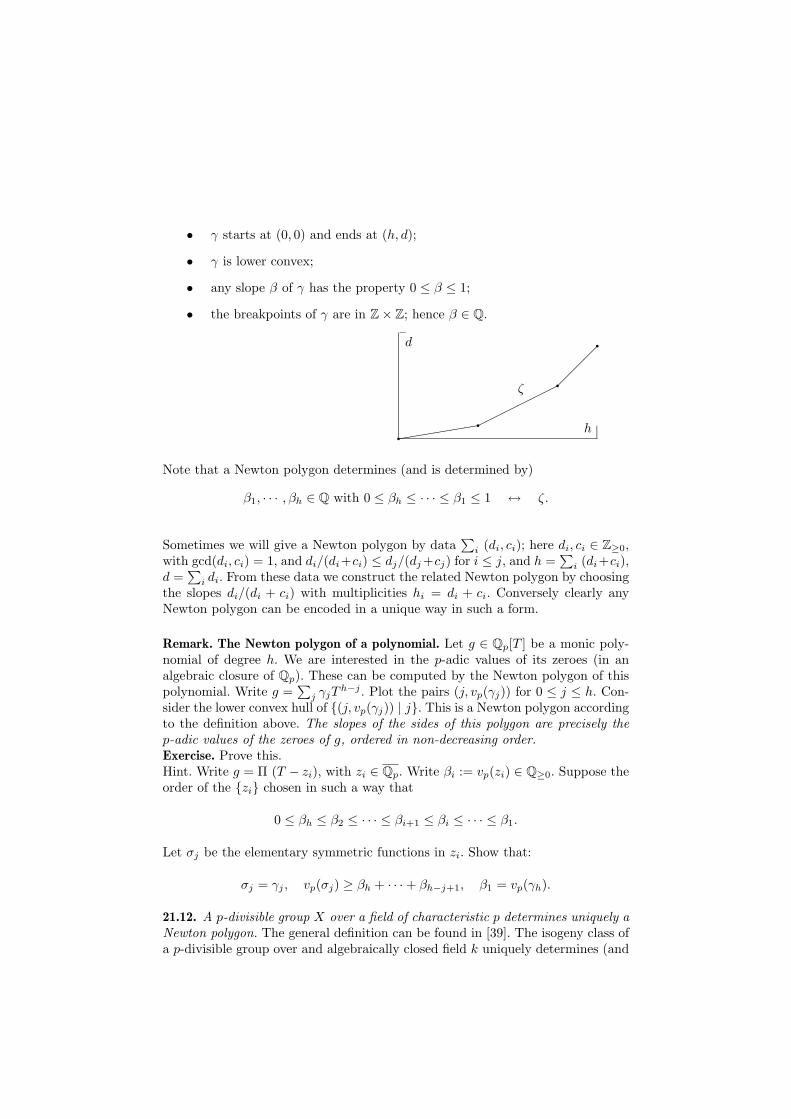
• γ starts at (0, 0) and ends at (h, d);

• γ is lower convex;

• any slope β of γ has the property 0 ≤ β ≤ 1;

• the breakpoints of γ are in Z× Z; hence β ∈ Q.

((((((

q qq

q

h

d

ζ

−

|

Note that a Newton polygon determines (and is determined by)

β1, · · · , βh ∈ Q with 0 ≤ βh ≤ · · · ≤ β1 ≤ 1 ↔ ζ.

Sometimes we will give a Newton polygon by data∑i (di, ci); here di, ci ∈ Z≥0,

with gcd(di, ci) = 1, and di/(di+ci) ≤ dj/(dj+cj) for i ≤ j, and h =∑i (di+ci),

d =∑i di. From these data we construct the related Newton polygon by choosing

the slopes di/(di + ci) with multiplicities hi = di + ci. Conversely clearly anyNewton polygon can be encoded in a unique way in such a form.

Remark. The Newton polygon of a polynomial. Let g ∈ Qp[T ] be a monic poly-nomial of degree h. We are interested in the p-adic values of its zeroes (in analgebraic closure of Qp). These can be computed by the Newton polygon of thispolynomial. Write g =

∑j γjT

h−j . Plot the pairs (j, vp(γj)) for 0 ≤ j ≤ h. Con-sider the lower convex hull of (j, vp(γj)) | j. This is a Newton polygon accordingto the definition above. The slopes of the sides of this polygon are precisely thep-adic values of the zeroes of g, ordered in non-decreasing order.Exercise. Prove this.Hint. Write g = Π (T − zi), with zi ∈ Qp. Write βi := vp(zi) ∈ Q≥0. Suppose theorder of the zi chosen in such a way that

0 ≤ βh ≤ β2 ≤ · · · ≤ βi+1 ≤ βi ≤ · · · ≤ β1.

Let σj be the elementary symmetric functions in zi. Show that:

σj = γj , vp(σj) ≥ βh + · · ·+ βh−j+1, β1 = vp(γh).

21.12. A p-divisible group X over a field of characteristic p determines uniquely aNewton polygon. The general definition can be found in [39]. The isogeny class ofa p-divisible group over and algebraically closed field k uniquely determines (and

is uniquely determined by) its Newton polygon. We use “the Newton polygon ofFrobenius”, a notion to be explained below.

21.13. Theorem (Dieudonne and Manin), see [39], “Classification theorem ” onpage 35 .

X/ ∼k∼−→ Newton polygon

21.14. We sketch the construction of a Newton polygon of a p-divisible group X,or of an abelian variety.

(Incorrect.) Here we indicate what the Newton polygon of a p-divisible group is(in a slightly incorrect way ...). Consider “the Frobenius endomorphism“ of X.This has a “characteristic polynomial”. This polynomial determines a Newtonpolygon, which we write as N (X), the Newton polygon of X. For an abelianvariety A we write N (A) instead of N (A[p∞]).

21.15. Exercise. Show that for an abelian variety A over the prime field Fp thisconstruction is valid, and does give the Newton polygon of A as defined in Section9.

Although, this “definition” is correct over Fp as ground field, over any other fieldF : X → X(p) is not an endomorphism, and the above “construction” fails.

21.16. Dieudonne-Manin theory. (We only give some definitions and facts.) Forcoprime integers d, c ∈ Z≥0 one can define a p-divisible group Gd,c. This is ap-divisible group of dimension d and of height d+ c. In fact, G1,0 = Gm[p∞], andG0,1 = (Qp/Zp). For d > 0 and c > 0 we have a formal p-divisible group Gd,cof dimension d and of height h = d + c. We do not give the construction here;see the first two chapters of Manin’s thesis [39]; the definition of Gd,c is on page35 of [39]. The p-divisible group Gd,c is defined over Fp; we will use the samesymbol for this group over any base field or base scheme over Fp, i.e. we writeGd,c instead of Gd,c ⊗Fp K. Moreover the p-divisible groups Gd,c and Gc,d overFp satisfy (Gd,c)t ∼= (Gc,d); here Xt denotes te Serre dual of X, see 8.3.Remark. With this defintion we have Gd,c[F d+c] = Gd,c[pd] and Gd,c[V d+c] =Gd,c[pc]

21.17. Exercise. Assume the existence of X = Gd,c over Fp as explained above.Let ζ be the Newton polygon of the Frobenius endomorphism of X. Show that ζconsists of d+ c slopes equal to d/(d+ c): this polygon is isoclinic (it is a straightline) and it ends at (d+ c, d).

Let K = Fpn , and X = Gd,c⊗FpK. Let πX ∈ End(X) be the geometric Frobenius.

Then

vp(πX) = d·nh , h := d+ c, q = pn.

21.18. In [39], Chapter II we find:Theorem. Let k be an algebraically closed field of characteristic p. Let X be ap-divisible group over k. Then there exists an isogeny

X ∼∏i

Gdi,ci .

See [39], Classification Theorem on page 35.

21.19. Definition of the Newton polygon of a p-divisible group. The isogeny classof

∏iGdi,ci will be encoded in the form of a Newton polygon. The simple p-

divisible group Gd,c will be represented by d + c slopes equal to d/(d + c). Theslopes of

∑iGdi,ci will be ordered in non-decreasing order. For a p-divisible group

of dimension d, height h with h = d + c together these slopes form a polygon inQ×Q.

For an abelian variety over a field of characteristic p we define N (A) :=N (A[p∞]).

Note that for a p-divisible group X over K its Newton polygon only dependson N (X ⊗ k), this only depends on the isogeny factors of X ⊗ k, and we canchoose these isogeny factors in such a way that they are defined over Fp.

Example. Suppose A[p∞] = X ∼ Gd,c×Gc,d. Then the Newton polygon N (A) ofA equals (d, c) + (c, d); this has d + c slopes equal to d/(d + c) and d + c slopesequal to c/(d+ c).

21.20. Definition. An abelian variety A over a field K ⊃ Fp is called supersingularif N (A) is isoclinic with all slopes equal to 1/2.Equivalently. An abelian variety A over a field K ⊃ Fp is supersingular if thereexists an isogeny (A⊗ k)[p∞] ∼ (G1,1)g.Exercise. Show that for an elliptic curve this definition and the one given in 21.8coincide.

Theorem (Tate, Shioda, Deligne, FO). An abelian variety A is supersingular iffthere exists a supersingular elliptic curve E and an isogeny A⊗ k ∼ Eg ⊗ k.See [72], Th. 2 on page 140, see [70], [52], Section 4.

21.21. Definition/Remark/Exercise. (1) Note that the definition of A being su-persingular can be given knowing only the p-divisible group A[p∞];

A is supersingular ⇐⇒ N (A) = σ,

where σ = g(1, 1) is the Newton polygon having only slopes equal to 1/2.Equivalently this definition can be given by the property in the theorem justmentioned.(2) We see that g > 1 and N (A) = σ imply that A is not absolutely simple.This is an exceptional case. Indeed, for any symmetric Newton polygon ξ 6= σand any p there exists an absolutely simple abelian variety A in characteristic p

with N (A) = ξ; see [36], see 18.13.(3) Let A be a simple abelian variety over the finite field Fq. Show:

A is supersingular ⇐⇒ πA ∼ ζ·√q,

where ζ is a root of unity.

21.22. Exercise. Let Y be a p-divisible group over a field K. Suppose Y ∼∏iGdi,ci

. Suppose there exist integers d, h ∈ Z>0 such that Y [Fh] = Y [pd]. Show:only factors Gdi,ci

do appear with di/(di + ci) = d/h.

21.23. Proposition. For every pair (d, c) of coprime non-negative integers we haveGd,c ∼= (Gc,d)t. Let A be an abelian variety over a field K ⊃ Fp, and X = A[p∞].The Newton polygon N (A) := N (X) is symmetric, in the sense of 11.1.Proof. The first equality follows from the definitions.

By 16.6 we have A[m]D = At[m] for every m ∈ Z>0. Hence A[p∞]t = At[p∞];use the definition of the Serre dual Xt; this formula is less trivial than notationsuggests. Hence Gd,cand Gc,d appear with the same multiplicity in the isogenytype of X = A[p∞]. This proves symmetry of N (X).

21.24. Remark. The theory as developed by Dieudonne and Manin gives theNewton polygon of a p-divisible group, and of an abelian variety over an arbitraryfield in characteristic p. Note that for an abelian variety an easier construction ispossible, which gives the same result, see Section 9, especially 9.3.

21.25. A proof for the Manin Conjecture. We have seen that the Manin Conjec-ture can be proved using the Honda-Tate theory, see Section 11. In [58], Section5 we find a proof of that conjecture, using only methods of characteristic p. Wesketch that proof (and please see the reference cited for notations and details).

We know that the conjecture holds for G1,1: in every characteristic p thereexists a supersingular elliptic curve, and E[p∞] ∼= G1,1. Hence every supersingularp-divisible group is algebraizable. We show that for a given g ≥ 1 there exists anabelian variety A0 with a principal polarization λ0 such that A0 is supersingular,and a(A0) = 1. Methods of [58] show that for a given symmetric Newton polygonξ, which automatically lies below σ = N (A0), there exists a formal deformationof (X0, λ0) = (A0, λ0)[p∞] to (X,λ) with N (X) = ξ. By the Serre-Tate Theo-rem we know that a formal deformation of an algebraizable p-divisible group isalgebraizable; hence there exists (A, λ) with (X,λ) = (A, λ)[p∞]; this proves theManin Conjecture.

22. Some questions

In this section we gather some remarks, questions and open problems.

22.1. Definition; see 12.2. Let B0 be an abelian variety over a field K of char-acteristic p > 0. We say B is a CM-lift of B0 if there exists an integral domainR of characteristic zero with a surjective homomorphism R K with field offractions Q(R) and an abelian scheme B → Spec(R) such that B ⊗K ∼= B0 andsuch that B ⊗Q(R) admits smCM.

Remarks. See Section 12. (1) If A0 admits a CM-lift, then A0⊗K admits smCM.(2) By Tate we know that any abelian variety over a finite field admits smCM,[72].(3) If A0 is an ordinary abelian variety over a finite field K, then by using thecanonical Serre-Tate lift we see that A0 admits a CM-lift.(4) Deuring has proved that any elliptic curve over a finite field admits a CM-lift;see [20], pp. 259 – 263; for a proof also see [55], Section 14, in particular 14.7.(5) The previous method can be used to show that any abelian variety of dimen-sion g defined over a finite field of p-rank equal to g − 1 admits a CM-lift; use[55], 14.6.(6) We have seen that for an abelian variety A0 over a finite field K there existsa finite extension K ⊂ K ′, and a K ′-isogeny A0 ⊗K ′ ∼ B0 such that B0 admitsa CM-lift.

Do we really need the finite extension and the isogeny to assure a CM-lift ?(7) (We need the isogeny.) In [56], Theorem B we find: suppose g ≥ 3, and let f bean integer, 0 ≤ f ≤ g − 2. Then there exists an abelian variety A0 over F := Fpof dimension g with p-rank equal to f such that A0 does not admit a CM-lift.

22.2. Question. (Do we need a finite extension?) Does there exist a finite field Kand an abelian variety A0 over K such that any B0 over K isogenous over Kwith A0 does not admit a CM-lift?

22.3. In the proof of the Honda-Tate theorem analytic tools are used. Indeed weconstruct CM abelian varieties over C in order to prove surjectivity of the mapA 7→ πA. As a corollary of the Honda-Tate theory we have seen a proof of theManin Conjecture. However it turns out that for the Manin Conjecture we nowhave a purely geometric proof, indeed a proof which only uses characteristic pmethods, see [58], Section 5.

22.4. Open Problem. Does there exist a proof of the Honda-Tate theorem 1.2 onlyusing methods in characteristic p ?

22.5. Over an algebraically closed field k of characteristic zero for a given g itis exactly known which algebras can appear as the endomorphism algebra of asimple abelian variety over k; see [68], pp. 175/176; also see [47], pp. 202/203; see[35], 5.5.

For any Albert algebra (an algebra of finite dimension over Q, with a posi-tive definite anti-involution, equivalently: a finite product of matrix algebras ofalgebras in the classification list of Albert), and any characteristic, there existsa simple abelian variety over an algebraically closed field of that characteristichaving that endomorphism algebra; see [68], pp. 175/176 and [47] pp. 202/203 forcharacteristic zero; for arbitrary characteristic see [24]; for a discussion see [54],Theorem 3.3 and Theorem 3.4.

22.6. Open Problem. Suppose a prime number p > 0 given. Determine for everyg ∈ Z>0 the possible endomorphism algebras appearing for that g in characteristicp.

22.7. Open Problem. For every characteristic and every g ∈ Z>0 determine allpossible endomorphism rings of an abelian variety over an algebraically closedfield in that characteristic.

22.8. Exercise. For an abelian variety of dimension g over a field K of charac-teristic zero we have

m(X) :=2g

[End0(A) : Q]∈ Z.

Give examples of an abelian variety A in positive characteristic where

2g[End0(A) : Q]

6∈ Z.

22.9. Expectation. For every γ ∈ Q>0 and every prime number p > 0 there existsa field k in characteristic p, and an abelian variety A over k such that

2g[End0(A) : Q]

= γ.

See [57], Section 2.

References

[1] A. A. Albert – On the construction of Riemann matrices, I, II. Ann. Math. 35 (1934), 1– 28; 36 (1935), 376 – 394.

[2] A. A. Albert – A solution of the principal problem in the theory of Riemann matrices.Ann. Math. 35 (1934), 500 – 515.

[3] A. A. Albert – Involutorial simple algebras and real Riemann matrices. Ann. Math. 36(1935), 886 – 964.

[4] C. Birkenhake & H. Lange – Complex tori. Progr. Math. 177, Birkhauser 1999.[5] A. Blanchard - Les corps non commutatifs. Coll. Sup, Presses Univ. France, 1972.[6] S. Bosch, W. Lutkebohmert & M. Raynaud – Neron models. Ergebn. Math. (3) Vol. 21,

Springer – Verlag 1990.[7] N. Bourbaki – Algebre. Chap.VIII: modules et anneaux semi-simples. Hermann, Paris

1985.[8] J. W. S. Cassels & A. Frohlich (Editors) – Algebraic number theory. Academic Press 1967.

Chapter VI: J-P. Serre – Local class field theory pp. 129–161.[9] C.-L. Chai & F. Oort – Hypersymmetric abelian varieties. Quarterly Journal of Pure and

Applied Mathematics, 2 (Special Issue: In honor of John H. Coates), (2006), 1–27.[10] C.-L. Chai & F. Oort – Moduli of abelian varieites and p-divisible groups. Conference

on arithmetic geometry, Gottingen July/August 2006. To appear: Clay Mathematics Pro-ceedings.

[11] C.-L. Chai, B. Conrad & F. Oort - CM-lifting of abelian varieties. [In preparation][12] C. Chevalley – Une demonstration d’un theoreme sur les groupes algebriques. Journ. de

Math. 39 (1960), 307 – 317.[13] B. Conrad – A modern proof of Chevalley’s theorem on algebraic groups. J. Ramanujan

Math. Soc. 18 (2002), 1 – 18.[14] B. Conrad – Chow’s K/k-image and K/k-trace, and the Lang-Neron theorem. Enseign.

Math. (2) 52 (2006), 37–108.[15] G. Cornell, J. H. Silverman (Editors) – Arithmetic geometry. Springer – Verlag 1986.

[16] C. W. Curtis & I. Reiner – Representation theory of finite groups and associative algebras.Intersc. Publ.1962.

[17] P. Deligne – Varietes abeliennes sur un corps fini. Invent. Math. 8 (1969), 238 – 243.[18] P. Deligne – Hodge cycles on abelian varieties. Hodge cycles, motives and Shimura varieties

(Eds P. Deligne et al). Lect. Notes Math. 900, Springer – Verlag 1982; pp. 9 - 100.[19] M. Demazure – Lectures on p-divisible groups. Lecture Notes Math. 302, Springer – Verlag

1972.[20] M. Deuring – Die Typen der Multiplikatorenringe elliptischer Funktionenkorper. Abh.

Math. Sem. Hamburg 14 (1941), 197 – 272.[21] G. Faltings – Endlichkeitssatze fur abelsche Varietaten uber Zahlkorpern. Invent. Math.

73 (1983), 349 – 366.[22] G. Faltings & G. Wustholz – Rational points. Seminar Bonn / Wuppertal 1983/84. Asp.

Math. E6, Vieweg 1984.[23] = [GM] G. van der Geer & B. Moonen – Abelian varieties. [In preparation] This will be

cited as [GM].[24] L. Gerritzen – On multiplications of Riemann matrices. Math. Ann 194 (1971), 109 – 122.[25] A. Grothendieck – Fondements de la geometrie algebrique. Extraits du Seminaire Bourbaki

1957 - 1962. Secr. math., Paris 1962.[26] A. Grothendieck – Groupes de Barsotti-Tate et cristaux de Dieudonne. Sem. Math. Sup.

45, Presses de l’Univ. de Montreal, 1970.[27] A. Grothendieck – Esquisse d’un programme. Manuscript 56 pp., January 1984. Re-

produced in: Geometric Galois actions (Ed. L. Schneps & P. Lochak). Vol. 1: AroundGrothendieck’s Esquisse d’un programme. London Math. Soc. Lect. Note Series 242, Cam-bridge Univ. Press 1997; pp. 5 – 48 (English translation pp. 243 – 283).http://www.institut.math.jussieu.fr/ leila/grothendieckcircle/EsquisseEng.pdf

[28] H. Hasse - Zahlentheorie. Akad. Verlag, Berlin 1949 (first printing, second printing 1963).[29] T. Honda – Isogeny classes of abelian varieties over finite fields. Journ. Math. Soc. Japan

20 (1968), 83 – 95.[30] A. J. de Jong – Homomorphisms of Barsotti-Tate groups and crystals in positive charac-

teristics. Invent. Math. 134 (1998) 301-333, Erratum 138 (1999) 225.[31] A. J. de Jong – Barsotti-Tate groups and crystals. Documenta Mathematica, Extra Volume

ICM 1998, II, 259 – 265.[32] N. M. Katz – Slope filtration of F–crystals. Journ. Geom. Alg. Rennes, Vol. I, Asterisque

63 (1979), Soc. Math. France, 113 - 164. are due to Tate[33] S. Lang – Fundamentals of diophantine geometry. Springer – Verlag 1983.[34] S. Lang – Complex multiplication. Grundl. math. Wissensch. 255, Springer – Verlag 1983.[35] H. Lange & C. Birkenhake - Complex abelian varieties. Grundl. math. Wissensch. 302,

Springer – Verlag 1992.[36] H. W. Lenstra jr & F. Oort – Simple abelian varieties having a prescribed formal isogeny

type. Journ. Pure Appl. Algebra 4 (1974), 47 - 53.[37] K.-Z. Li & F. Oort – Moduli of supersingular abelian varieties. Lecture Notes Math. 1680,

Springer - Verlag 1998.[38] J. Lubin & J. Tate – . Formal moduli for one-parameter formal Lie groups. Bull. Soc.

Math. France 94 (1966), 49 – 66.[39] Yu. I. Manin – The theory of commutative formal groups over fields of finite characteristic.

Usp. Math. 18 (1963), 3-90; Russ. Math. Surveys 18 (1963), 1-80.[40] J. Milne – it The fundamental theorem of complex multiplication.

arXiv:0705.3446v1, 23 May 2007[41] S. Mochizuki – The local pro-p anabelian geometry of curves. Invent. Math. 138 (1999),

319 – 423.[42] L. Moret-Bailly – Pinceaux de varietes abeliennes. Asterisque 129. Soc. Math. France

1985.[43] S. Mori – On Tate’s conjecture concerning endomorphisms of abelian varieties. Itl. Sym-

pos. Algebr. Geom. Kyoto 1977 (Ed. M. Nagata). Kinokuniya Book-store 1987, pp. 219 -230.

[44] D. Mumford – A note of Shimura’s paper “Discontinuous groups and abelian varieties”.

Math. Ann. 181 (1969), 345 - 351.[45] D. Mumford – Geometric invariant theory. Ergebn. Math. Vol. 34, Springer – Verlag 1965

(second version 1982, 1994).[46] D. Mumford - A note of Shimura’s paper “Discontinuous groups and abelian varieties”.

Math. Ann. 181 (1969), 345-351.[47] D. Mumford – Abelian varieties. Tata Inst. Fund. Research and Oxford Univ. Press 1970

(2nd printing 1974).[48] A. Neron – Modeles minimaux des varietes abeliennes sur les corps locaux et globaux.

Publ. Math. IHES 21, 1964.[49] F. Oort – Commutative group schemes. Lect. Notes Math. 15, Springer - Verlag 1966.[50] F. Oort – Algebraic group schemes in characteristic zero are reduced. Invent. Math. 2

(1966), 79 - 80.[51] F. Oort – The isogeny class of a CM-type abelian variety is defined over a finite extension

of the prime field. Journ. Pure Appl. Algebra 3 (1973), 399 - 408.[52] F. Oort – Subvarieties of moduli spaces. Invent. Math. 24 (1974), 95 - 119.[53] F. Oort – Good and stable reduction of abelian varieties. Manuscr. Math. 11 (1974), 171

- 197.[54] F. Oort – Endomorphism algebras of abelian varieties. Algebraic Geometry and Commut.

Algebra in honor of M. Nagata (Ed. H. Hijikata et al), Kinokuniya Cy Tokyo, Japan, 1988,Vol II; pp. 469 - 502.

[55] F. Oort – — Lifting algebraic curves, abelian varieties and their endomorphisms to char-acteristic zero. Algebraic Geometry, Bowdoin 1985 (Ed. S. J. Bloch). Proceed. Sympos.Pure Math. 46 Part 2, AMS 1987; pp. 165 -195.

[56] F. Oort – CM-liftings of abelian varieties. Journ. Algebraic Geometry 1 (1992), 131 - 146.[57] F. Oort – Some questions in algebraic geometry, preliminary version. Manuscript, June

1995. http://www.math.uu.nl/people/oort/[58] F. Oort — Newton polygons and formal groups: conjectures by Manin and Grothendieck.

Ann. Math. 152 (2000), 183 - 206.[59] F. Oort – Newton polygon strata in the moduli space of abelian varieties. In: Moduli of

abelian varieties. (Ed. C. Faber, G. van der Geer, F. Oort). Progress Math. 195, BirkhauserVerlag 2001; pp. 417 - 440.

[60] F. Oort & Yu. G. Zarhin - Endomorphism algebras of complex tori. Math. Ann. 303 (1995),11 - 29.

[61] I. Reiner – Maximal orders. London Math. Soc. Monographs Vol. 28. Oxford 2003.[62] M. Demazure & A. Grothendieck – Schemas en groupes, Seminaire de geometrie

algebrique, SGA3. Vol I: Lect. Notes Math. 151, Springer – Verlag 1970.[63] A. Grothendieck – Seminaire de Geometrie Algebrique, Groupes de monodromie en

geometrie algebrique, SGA 7. Lect. Notes Math. 288, Springer – Verlag 1972.[64] R. Schoof – Nonsingular plane cubic curves over finite fields. Journal Computat. Theory,

Series A, 46 (1987) 183 – 211.[65] J-P. Serre – Corps locaux. Hermann Paris 1962.[66] J-P. Serre – Geometrie algebrique et geometrie analytique. Ann. Inst. Fourier 6) (1956),

1 – 42.[67] J-P. Serre & J. Tate – Good reduction of abelian varieties. Ann. Math. 88 (1968), 492 –

517.[68] G. Shimura – On analytic families of polarized abelian varieties and automorphic func-

tions. Ann. Math. 78 (1963), 149 – 193.[69] G. Shimura & Y. Taniyama – Complex multiplication of abelian varieties and its applica-

tions to number theory. Publ. Math. Soc. Japan 6, Tokyo 1961.[70] T. Shioda – Supersingular K3 surfaces. In: Algebraic Geometry, Copenhagen 1978 (Ed.

K. Lønsted). Lect. Notes Math. 732, Springer - Verlag (1979), 564 - 591.[71] J. Silverman – The arithmetic of elliptic curves. Grad. Texts Math. 106, Springer – Verlag,

1986.[72] J. Tate – Endomorphisms of abelian varieties over finite fields. Invent. Math. 2 (1966),

134-144.[73] J. Tate – Classes d’isogenies de varietes abeliennes sur un corps fini (d’apres T. Honda).

Sem. Bourbaki 21 (1968/69), Exp. 352.[74] 2005-05 VIGRE number theory working group. Organized by Brian Conrad and Chris

Skinner. On: http://www.math.Isa.umich.edu/ bdconrad/vigre04.html[75] W. C. Waterhouse – Abelian varieties over finite fields. Ann. Sc. Ec. Norm. Sup. 4.Ser, 2

(1969), 521 – 560).[76] W. C. Waterhouse – Introduction to affine group schemes. Grad. Texts Math. 66, Springer

– Verlag, 1979.[77] W. C. Waterhouse & J. S. Milne – Abelian varieties over finite fields. Proc. Sympos. pure

math. Vol. XX, 1969 Number Theory Institute (Stony Brook), AMS 1971, pp. 53 – 64.[78] A. Weil – Sur les courbes algebriques et les varietes qui s’en deduisent. Hermann, 1948.[79] A. Weil – Varietes abeliennes et courbes algebriques. Hermann, 1948.[80] C.-F. Yu – The isomorphism classes of abelian varieties of CM-type. Journ. Pure Appl.

Algebra 187 (2004), 305 – 319.[81] J. G. Zarhin – Isogenies of abelian varieties over fields of finite characteristic. Math.

USSR Sbornik 24 (1974), 451 – 461.[82] J. G. Zarhin – A remark on endomorphisms of abelian varieties over function fields of

finite characteristic. Math. USSR Izv. 8 (1974), 477 – 480.[83] J. G. Zarhin – Homomorphisms of abelian varieties over finite fields. Summer school in

Gottingen, June 2007. See this volume.