ABC 40 -90 A mixture of monoammoniumphosphate and ammoniumsulphate with mineral additives.
Upload
christian-robertCategory
view
2.013download
0
ABCD: ABC in High Dimensions
Christian P. Robert
Universite Paris-Dauphine, University of Warwick, & IUF
workshop 17w5025, BIRS, Banff, Alberta, Canada
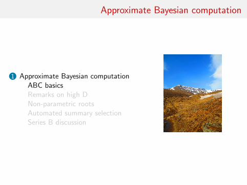
Approximate Bayesian computation
1 Approximate Bayesian computationABC basicsRemarks on high DNon-parametric rootsAutomated summary selectionSeries B discussion
The ABC method
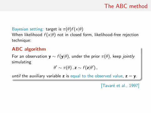
Bayesian setting: target is π(θ)f (x |θ)
When likelihood f (x |θ) not in closed form, likelihood-free rejectiontechnique:
ABC algorithm
For an observation y ∼ f (y|θ), under the prior π(θ), keep jointlysimulating
θ′ ∼ π(θ) , z ∼ f (z|θ′) ,
until the auxiliary variable z is equal to the observed value, z = y.
[Tavare et al., 1997]
The ABC method
Bayesian setting: target is π(θ)f (x |θ)When likelihood f (x |θ) not in closed form, likelihood-free rejectiontechnique:
ABC algorithm
For an observation y ∼ f (y|θ), under the prior π(θ), keep jointlysimulating
θ′ ∼ π(θ) , z ∼ f (z|θ′) ,
until the auxiliary variable z is equal to the observed value, z = y.
[Tavare et al., 1997]
A as A...pproximative
When y is a continuous random variable, equality z = y is replacedwith a tolerance condition,
%(y, z) ≤ ε
where % is a distance
Output distributed from
π(θ)Pθ{%(y, z) < ε} ∝ π(θ|%(y, z) < ε)
[Pritchard et al., 1999]
A as A...pproximative
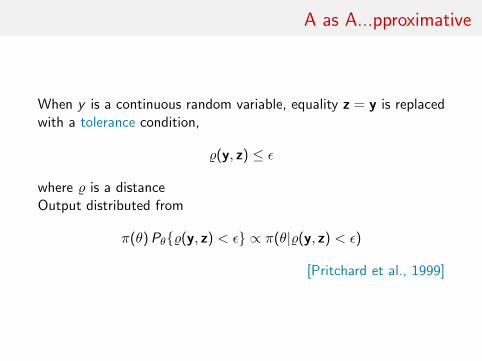
When y is a continuous random variable, equality z = y is replacedwith a tolerance condition,
%(y, z) ≤ ε
where % is a distanceOutput distributed from
π(θ)Pθ{%(y, z) < ε} ∝ π(θ|%(y, z) < ε)
[Pritchard et al., 1999]
ABC algorithm
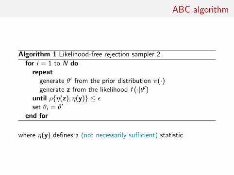
Algorithm 1 Likelihood-free rejection sampler 2
for i = 1 to N dorepeat
generate θ′ from the prior distribution π(·)generate z from the likelihood f (·|θ′)
until ρ{η(z), η(y)} ≤ εset θi = θ′
end for
where η(y) defines a (not necessarily sufficient) statistic
Output
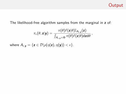
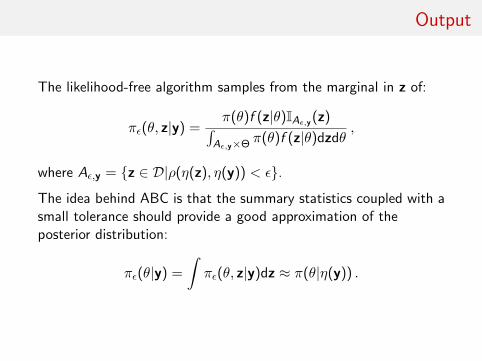
The likelihood-free algorithm samples from the marginal in z of:
πε(θ, z|y) =π(θ)f (z|θ)IAε,y (z)∫
Aε,y×Θ π(θ)f (z|θ)dzdθ,
where Aε,y = {z ∈ D|ρ(η(z), η(y)) < ε}.
The idea behind ABC is that the summary statistics coupled with asmall tolerance should provide a good approximation of theposterior distribution:
πε(θ|y) =
∫πε(θ, z|y)dz ≈ π(θ|η(y)) .
Output
The likelihood-free algorithm samples from the marginal in z of:
πε(θ, z|y) =π(θ)f (z|θ)IAε,y (z)∫
Aε,y×Θ π(θ)f (z|θ)dzdθ,
where Aε,y = {z ∈ D|ρ(η(z), η(y)) < ε}.
The idea behind ABC is that the summary statistics coupled with asmall tolerance should provide a good approximation of theposterior distribution:
πε(θ|y) =
∫πε(θ, z|y)dz ≈ π(θ|η(y)) .
MA example
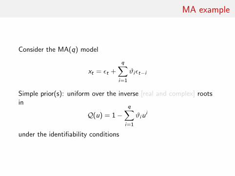
Consider the MA(q) model
xt = εt +
q∑i=1
ϑiεt−i
Simple prior(s): uniform over the inverse [real and complex] rootsin
Q(u) = 1−q∑
i=1
ϑiui
under the identifiability conditions
MA example
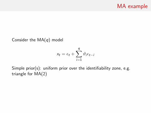
Consider the MA(q) model
xt = εt +
q∑i=1
ϑiεt−i
Simple prior(s): uniform prior over the identifiability zone, e.g.triangle for MA(2)
MA example (2)
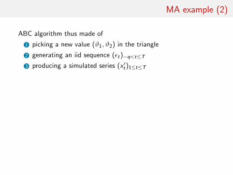
ABC algorithm thus made of
1 picking a new value (ϑ1, ϑ2) in the triangle
2 generating an iid sequence (εt)−q<t≤T
3 producing a simulated series (x ′t)1≤t≤T
Distance: basic distance between the series
ρ((x ′t)1≤t≤T , (xt)1≤t≤T ) =T∑t=1
(xt − x ′t)2
or distance between summary statistics like the q autocorrelations
τj =T∑
t=j+1
xtxt−j
MA example (2)
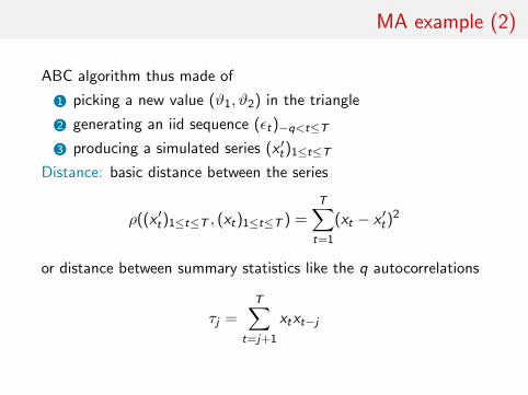
ABC algorithm thus made of
1 picking a new value (ϑ1, ϑ2) in the triangle
2 generating an iid sequence (εt)−q<t≤T
3 producing a simulated series (x ′t)1≤t≤T
Distance: basic distance between the series
ρ((x ′t)1≤t≤T , (xt)1≤t≤T ) =T∑t=1
(xt − x ′t)2
or distance between summary statistics like the q autocorrelations
τj =T∑
t=j+1
xtxt−j
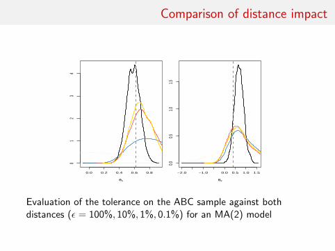
Comparison of distance impact
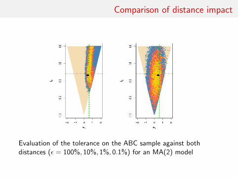
Evaluation of the tolerance on the ABC sample against bothdistances (ε = 100%, 10%, 1%, 0.1%) for an MA(2) model
Comparison of distance impact
0.0 0.2 0.4 0.6 0.8
01
23
4
θ1
−2.0 −1.0 0.0 0.5 1.0 1.50.0
0.51.0
1.5
θ2
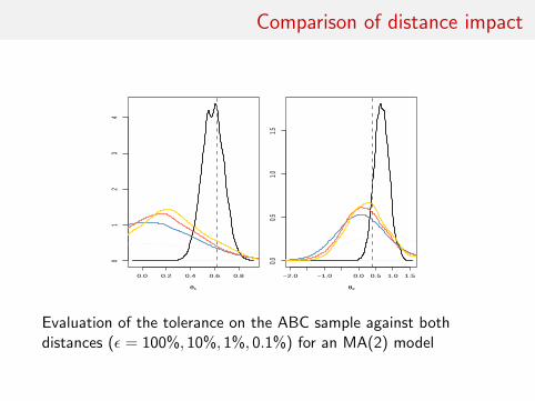
Evaluation of the tolerance on the ABC sample against bothdistances (ε = 100%, 10%, 1%, 0.1%) for an MA(2) model
Comparison of distance impact
0.0 0.2 0.4 0.6 0.8
01
23
4
θ1
−2.0 −1.0 0.0 0.5 1.0 1.50.0
0.51.0
1.5
θ2
Evaluation of the tolerance on the ABC sample against bothdistances (ε = 100%, 10%, 1%, 0.1%) for an MA(2) model
Approximate Bayesian computation
1 Approximate Bayesian computationABC basicsRemarks on high DNon-parametric rootsAutomated summary selectionSeries B discussion
ABC[and the]D[curse]
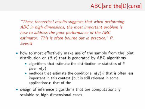
“These theoretical results suggests that when performingABC in high dimensions, the most important problem ishow to address the poor performance of the ABCestimator. This is often bourne out in practice.” R.Everitt
• how to most effectively make use of the sample from the jointdistribution on (θ, t) that is generated by ABC algorithms• algorithms that estimate the distribution or statistics of θ
given η(y)• methods that estimate the conditional η(y)|θ that is often less
important in this context (but is still relevant in someapplications): that of the
• design of inference algorithms that are computationallyscalable to high dimensional cases
Parameter given summary
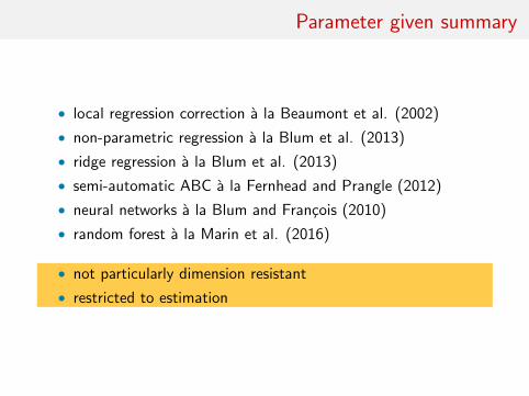
• local regression correction a la Beaumont et al. (2002)
• non-parametric regression a la Blum et al. (2013)
• ridge regression a la Blum et al. (2013)
• semi-automatic ABC a la Fernhead and Prangle (2012)
• neural networks a la Blum and Francois (2010)
• random forest a la Marin et al. (2016)
• not particularly dimension resistant
• restricted to estimation
Summary given parameter
• non-parametric regression a la Blum et al. (2013)
• synthetic likelihood a la Wood (2010) and Dutta et al. (2016)
• Gaussian processes a la Wilkinson (2014), Meeds and Welling(2013), Jarvenpaa et al. (2016)
Reproducing kernel Hilbert spaces
Several papers suggesting moving from kernel estimation to RKHSregression:
• Fukumizu, Le & Gretton (2013)
• Nakagome, Fukumizu, & Mano (2013)
• Park, Jitkrittum, & Sejdinovic (2016)
• Mitrovic, Sejdinovic, & Teh (2016)
Reproducing kernel Hilbert spaces
Several papers suggesting moving from kernel estimation to RKHSregression:with arguments
• removing dependence on summary statistics by using “thedata themselves”
• correlatively no loss of information
• providing a form of distance between empirical measures
• learning directly the regression
• relatively easy and fast implementation (with linear timeMMD)
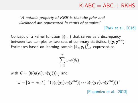
K-ABC = ABC + RKHS
”A notable property of KBR is that the prior andlikelihood are represented in terms of samples.”
[Park et al., 2016]
Concept of a kernel function h(·, ·) that serves as a discrepancybetween two samples or two sets of summary statistics, h(y, yobs)
Estimates based on learning sample (θt , yt)Tt=1 expressed as
T∑t=1
ωth(θt)
with G = (h(η(yi ), η(yj)))i ,j and
ω = [G + nεnIn]−1(h(η(y1), η(yobs)) · · · h(η(yT ), η(yobs)))T
[Fukumizu et al., 2013]
K-ABC = ABC + RKHS
”A notable property of KBR is that the prior andlikelihood are represented in terms of samples.”
[Park et al., 2016]
Concept of a kernel function h(·, ·) that serves as a discrepancybetween two samples or two sets of summary statistics, h(y, yobs)Estimates based on learning sample (θt , yt)Tt=1 expressed as
T∑t=1
ωth(θt)
with G = (h(η(yi ), η(yj)))i ,j and
ω = [G + nεnIn]−1(h(η(y1), η(yobs)) · · · h(η(yT ), η(yobs)))T
[Fukumizu et al., 2013]
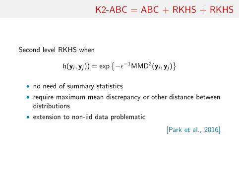
K2-ABC = ABC + RKHS + RKHS
Second level RKHS when
h(yi , yj)) = exp{−ε−1MMD2(yi , yj)
}• no need of summary statistics
• require maximum mean discrepancy or other distance betweendistributions
• extension to non-iid data problematic
[Park et al., 2016]
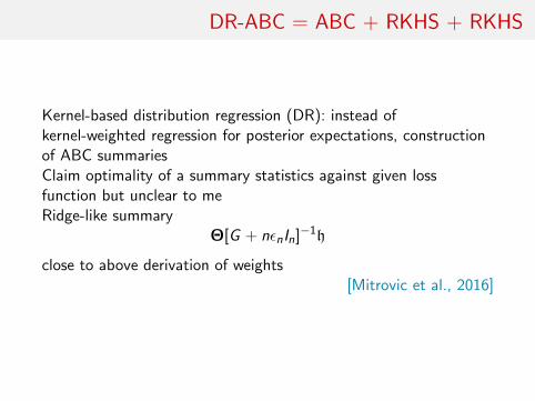
DR-ABC = ABC + RKHS + RKHS
Kernel-based distribution regression (DR): instead ofkernel-weighted regression for posterior expectations, constructionof ABC summariesClaim optimality of a summary statistics against given lossfunction but unclear to meRidge-like summary
Θ[G + nεnIn]−1h
close to above derivation of weights[Mitrovic et al., 2016]
Approximate Bayesian computation
1 Approximate Bayesian computationABC basicsRemarks on high DNon-parametric rootsAutomated summary selectionSeries B discussion
ABC-NP
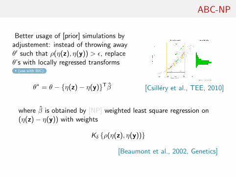
Better usage of [prior] simulations byadjustement: instead of throwing awayθ′ such that ρ(η(z), η(y)) > ε, replaceθ’s with locally regressed transforms
(use with BIC)
θ∗ = θ − {η(z)− η(y)}Tβ [Csillery et al., TEE, 2010]
where β is obtained by [NP] weighted least square regression on(η(z)− η(y)) with weights
Kδ {ρ(η(z), η(y))}
[Beaumont et al., 2002, Genetics]
ABC-NP (regression)
Also found in the subsequent literature, e.g. in Fearnhead-Prangle (2012) :weight directly simulation by
Kδ {ρ(η(z(θ)), η(y))}
or
1
S
S∑s=1
Kδ {ρ(η(zs(θ)), η(y))}
[consistent estimate of f (η|θ)]
Curse of dimensionality: poor estimate when d = dim(η) is large...
ABC-NP (regression)
Also found in the subsequent literature, e.g. in Fearnhead-Prangle (2012) :weight directly simulation by
Kδ {ρ(η(z(θ)), η(y))}
or
1
S
S∑s=1
Kδ {ρ(η(zs(θ)), η(y))}
[consistent estimate of f (η|θ)]
Curse of dimensionality: poor estimate when d = dim(η) is large...
ABC-NP (density estimation)
Use of the kernel weights
Kδ {ρ(η(z(θ)), η(y))}
leads to the NP estimate of the posterior expectation∑i θiKδ {ρ(η(z(θi )), η(y))}∑i Kδ {ρ(η(z(θi )), η(y))}
[Blum, JASA, 2010]
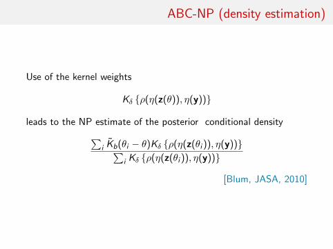
ABC-NP (density estimation)
Use of the kernel weights
Kδ {ρ(η(z(θ)), η(y))}
leads to the NP estimate of the posterior conditional density∑i Kb(θi − θ)Kδ {ρ(η(z(θi )), η(y))}∑
i Kδ {ρ(η(z(θi )), η(y))}
[Blum, JASA, 2010]
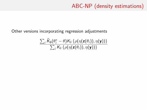
ABC-NP (density estimations)
Other versions incorporating regression adjustments∑i Kb(θ∗i − θ)Kδ {ρ(η(z(θi )), η(y))}∑
i Kδ {ρ(η(z(θi )), η(y))}
In all cases, error
E[g(θ|y)]− g(θ|y) = cb2 + cδ2 + OP(b2 + δ2) + OP(1/nδd)
var(g(θ|y)) =c
nbδd(1 + oP(1))
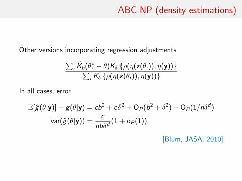
ABC-NP (density estimations)
Other versions incorporating regression adjustments∑i Kb(θ∗i − θ)Kδ {ρ(η(z(θi )), η(y))}∑
i Kδ {ρ(η(z(θi )), η(y))}
In all cases, error
E[g(θ|y)]− g(θ|y) = cb2 + cδ2 + OP(b2 + δ2) + OP(1/nδd)
var(g(θ|y)) =c
nbδd(1 + oP(1))
[Blum, JASA, 2010]
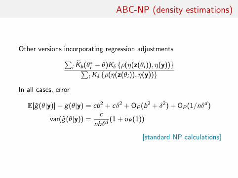
ABC-NP (density estimations)
Other versions incorporating regression adjustments∑i Kb(θ∗i − θ)Kδ {ρ(η(z(θi )), η(y))}∑
i Kδ {ρ(η(z(θi )), η(y))}
In all cases, error
E[g(θ|y)]− g(θ|y) = cb2 + cδ2 + OP(b2 + δ2) + OP(1/nδd)
var(g(θ|y)) =c
nbδd(1 + oP(1))
[standard NP calculations]
ABC-NCH
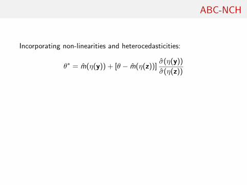
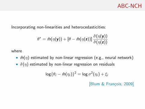
Incorporating non-linearities and heterocedasticities:
θ∗ = m(η(y)) + [θ − m(η(z))]σ(η(y))
σ(η(z))
where
• m(η) estimated by non-linear regression (e.g., neural network)
• σ(η) estimated by non-linear regression on residuals
log{θi − m(ηi )}2 = log σ2(ηi ) + ξi
[Blum & Francois, 2009]
ABC-NCH
Incorporating non-linearities and heterocedasticities:
θ∗ = m(η(y)) + [θ − m(η(z))]σ(η(y))
σ(η(z))
where
• m(η) estimated by non-linear regression (e.g., neural network)
• σ(η) estimated by non-linear regression on residuals
log{θi − m(ηi )}2 = log σ2(ηi ) + ξi
[Blum & Francois, 2009]

ABC-NCH (2)
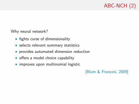
Why neural network?
• fights curse of dimensionality
• selects relevant summary statistics
• provides automated dimension reduction
• offers a model choice capability
• improves upon multinomial logistic
[Blum & Francois, 2009]
ABC-NCH (2)
Why neural network?
• fights curse of dimensionality
• selects relevant summary statistics
• provides automated dimension reduction
• offers a model choice capability
• improves upon multinomial logistic
[Blum & Francois, 2009]
ABC as knn
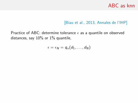
[Biau et al., 2013, Annales de l’IHP]
Practice of ABC: determine tolerance ε as a quantile on observeddistances, say 10% or 1% quantile,
ε = εN = qα(d1, . . . , dN)
• Interpretation of ε as nonparametric bandwidth onlyapproximation of the actual practice
[Blum & Francois, 2010]
• ABC is a k-nearest neighbour (knn) method with kN = NεN[Loftsgaarden & Quesenberry, 1965]
ABC as knn
[Biau et al., 2013, Annales de l’IHP]
Practice of ABC: determine tolerance ε as a quantile on observeddistances, say 10% or 1% quantile,
ε = εN = qα(d1, . . . , dN)
• Interpretation of ε as nonparametric bandwidth onlyapproximation of the actual practice
[Blum & Francois, 2010]
• ABC is a k-nearest neighbour (knn) method with kN = NεN[Loftsgaarden & Quesenberry, 1965]

ABC consistency
Provided
kN/ log logN −→∞ and kN/N −→ 0
as N →∞, for almost all s0 (with respect to the distribution ofS), with probability 1,
1
kN
kN∑j=1
ϕ(θj) −→ E[ϕ(θj)|S = s0]
[Devroye, 1982]
Biau et al. (2013) also recall pointwise and integrated mean square errorconsistency results on the corresponding kernel estimate of theconditional posterior distribution, under constraints
kN →∞, kN/N → 0, hN → 0 and hpNkN →∞,
Rates of convergence
Further assumptions (on target and kernel) allow for precise(integrated mean square) convergence rates (as a power of thesample size N), derived from classical k-nearest neighbourregression, like
• when m = 1, 2, 3, kN ≈ N(p+4)/(p+8) and rate N−4
p+8
• when m = 4, kN ≈ N(p+4)/(p+8) and rate N−4
p+8 logN
• when m > 4, kN ≈ N(p+4)/(m+p+4) and rate N−4
m+p+4
[Biau et al., 2013]
Noisy ABC
Idea: Modify the data from the start
y = y0 + εζ1
with the same scale ε as ABC[ see Fearnhead-Prangle ] and
run ABC on y
Then ABC produces an exact simulation from π(θ|y) = π(θ|y)[Dean et al., 2011; Fearnhead and Prangle, 2012]
Noisy ABC
Idea: Modify the data from the start
y = y0 + εζ1
with the same scale ε as ABC[ see Fearnhead-Prangle ] and
run ABC on yThen ABC produces an exact simulation from π(θ|y) = π(θ|y)
[Dean et al., 2011; Fearnhead and Prangle, 2012]
Consistent noisy ABC
• Degrading the data improves the estimation performances:• Noisy ABC-MLE is asymptotically (in n) consistent• under further assumptions, the noisy ABC-MLE is
asymptotically normal• increase in variance of order ε−2
• likely degradation in precision or computing time due to thelack of summary statistic [curse of dimensionality]
Approximate Bayesian computation
1 Approximate Bayesian computationABC basicsRemarks on high DNon-parametric rootsAutomated summary selectionSeries B discussion
Semi-automatic ABC
Fearnhead and Prangle (2010) study ABC and the selection of thesummary statistic in close proximity to Wilkinson’s proposal
ABC then considered from a purely inferential viewpoint andcalibrated for estimation purposesUse of a randomised (or ‘noisy’) version of the summary statistics
η(y) = η(y) + τε
Derivation of a well-calibrated version of ABC, i.e. an algorithmthat gives proper predictions for the distribution associated withthis randomised summary statistic
[calibration constraint: ABCapproximation with same posterior mean as the true randomisedposterior]
Semi-automatic ABC
Fearnhead and Prangle (2010) study ABC and the selection of thesummary statistic in close proximity to Wilkinson’s proposal
ABC then considered from a purely inferential viewpoint andcalibrated for estimation purposesUse of a randomised (or ‘noisy’) version of the summary statistics
η(y) = η(y) + τε
Derivation of a well-calibrated version of ABC, i.e. an algorithmthat gives proper predictions for the distribution associated withthis randomised summary statistic [calibration constraint: ABCapproximation with same posterior mean as the true randomisedposterior]
Summary statistics
• Optimality of the posterior expectation E[θ|y] of theparameter of interest as summary statistics η(y)!
• Use of the standard quadratic loss function
(θ − θ0)TA(θ − θ0) .
bare summary
Summary statistics
• Optimality of the posterior expectation E[θ|y] of theparameter of interest as summary statistics η(y)!
• Use of the standard quadratic loss function
(θ − θ0)TA(θ − θ0) .
bare summary
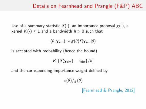
Details on Fearnhead and Prangle (F&P) ABC
Use of a summary statistic S(·), an importance proposal g(·), akernel K (·) ≤ 1 and a bandwidth h > 0 such that
(θ, ysim) ∼ g(θ)f (ysim|θ)
is accepted with probability (hence the bound)
K [{S(ysim)− sobs}/h]
and the corresponding importance weight defined by
π(θ)/g(θ)
[Fearnhead & Prangle, 2012]
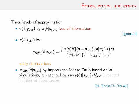
Errors, errors, and errors
Three levels of approximation
• π(θ|yobs) by π(θ|sobs) loss of information[ignored]
• π(θ|sobs) by
πABC(θ|sobs) =
∫π(s)K [{s− sobs}/h]π(θ|s) ds∫π(s)K [{s− sobs}/h] ds
noisy observations
• πABC(θ|sobs) by importance Monte Carlo based on Nsimulations, represented by var(a(θ)|sobs)/Nacc [expectednumber of acceptances]
[M. Twain/B. Disraeli]
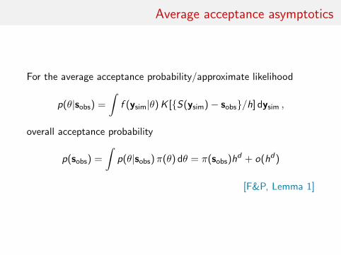
Average acceptance asymptotics
For the average acceptance probability/approximate likelihood
p(θ|sobs) =
∫f (ysim|θ)K [{S(ysim)− sobs}/h] dysim ,
overall acceptance probability
p(sobs) =
∫p(θ|sobs)π(θ) dθ = π(sobs)h
d + o(hd)
[F&P, Lemma 1]
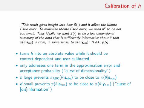
Calibration of h
“This result gives insight into how S(·) and h affect the MonteCarlo error. To minimize Monte Carlo error, we need hd to be nottoo small. Thus ideally we want S(·) to be a low dimensionalsummary of the data that is sufficiently informative about θ thatπ(θ|sobs) is close, in some sense, to π(θ|yobs)” (F&P, p.5)
• turns h into an absolute value while it should becontext-dependent and user-calibrated
• only addresses one term in the approximation error andacceptance probability (“curse of dimensionality”)
• h large prevents πABC(θ|sobs) to be close to π(θ|sobs)
• d small prevents π(θ|sobs) to be close to π(θ|yobs) (“curse of[dis]information”)
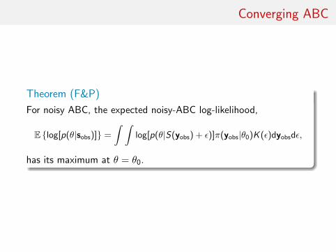
Converging ABC
Theorem (F&P)
For noisy ABC, the expected noisy-ABC log-likelihood,
E {log[p(θ|sobs)]} =
∫ ∫log[p(θ|S(yobs) + ε)]π(yobs|θ0)K (ε)dyobsdε,
has its maximum at θ = θ0.
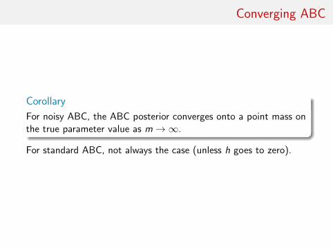
Converging ABC
Corollary
For noisy ABC, the ABC posterior converges onto a point mass onthe true parameter value as m→∞.
For standard ABC, not always the case (unless h goes to zero).
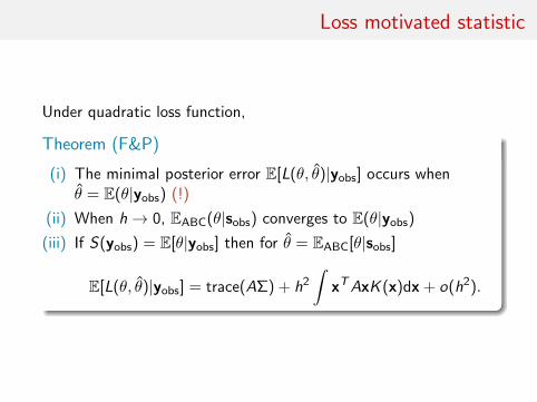
Loss motivated statistic
Under quadratic loss function,
Theorem (F&P)
(i) The minimal posterior error E[L(θ, θ)|yobs] occurs whenθ = E(θ|yobs) (!)
(ii) When h→ 0, EABC(θ|sobs) converges to E(θ|yobs)
(iii) If S(yobs) = E[θ|yobs] then for θ = EABC[θ|sobs]
E[L(θ, θ)|yobs] = trace(AΣ) + h2
∫xTAxK (x)dx + o(h2).
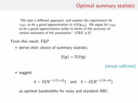
Optimal summary statistic
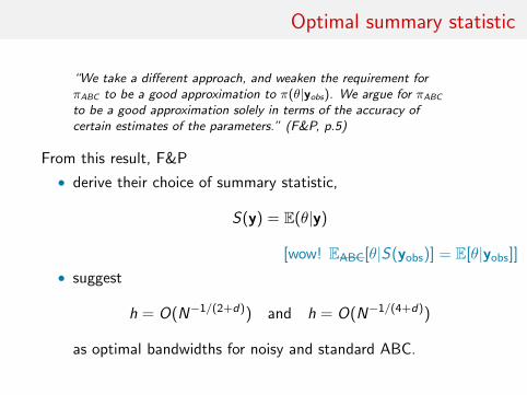
“We take a different approach, and weaken the requirement forπABC to be a good approximation to π(θ|yobs). We argue for πABC
to be a good approximation solely in terms of the accuracy ofcertain estimates of the parameters.” (F&P, p.5)
From this result, F&P
• derive their choice of summary statistic,
S(y) = E(θ|y)
[almost sufficient]
• suggest
h = O(N−1/(2+d)) and h = O(N−1/(4+d))
as optimal bandwidths for noisy and standard ABC.
Optimal summary statistic
“We take a different approach, and weaken the requirement forπABC to be a good approximation to π(θ|yobs). We argue for πABC
to be a good approximation solely in terms of the accuracy ofcertain estimates of the parameters.” (F&P, p.5)
From this result, F&P
• derive their choice of summary statistic,
S(y) = E(θ|y)
[wow! EABC[θ|S(yobs)] = E[θ|yobs]]
• suggest
h = O(N−1/(2+d)) and h = O(N−1/(4+d))
as optimal bandwidths for noisy and standard ABC.
Caveat
Since E(θ|yobs) is most usuallyunavailable, F&P suggest
(i) use a pilot run of ABC todetermine a region ofnon-negligible posterior mass;
(ii) simulate sets of parametervalues and data;
(iii) use the simulated sets ofparameter values and data toestimate the summary statistic;and
(iv) run ABC with this choice ofsummary statistic.
Approximate Bayesian computation
1 Approximate Bayesian computationABC basicsRemarks on high DNon-parametric rootsAutomated summary selectionSeries B discussion
More discussions about semi-automatic ABC
[ End of section derived from comments on Read Paper, Series B, 2012]
“The apparently arbitrary nature of the choice of summary statisticshas always been perceived as the Achilles heel of ABC.” M.Beaumont
• “Curse of dimensionality” linked with the increase of thedimension of the summary statistic
• Connection with principal component analysis[Itan et al., 2010]
• Connection with partial least squares[Wegman et al., 2009]
• Beaumont et al. (2002) postprocessed output is used as inputby F&P to run a second ABC

Wood’s alternative
Instead of a non-parametric kernel approximation to the likelihood
1
R
∑r
Kε{η(yr )− η(yobs)}
Wood (2010) suggests a normal approximation
η(y(θ)) ∼ Nd(µθ,Σθ)
whose parameters can be approximated based on the R simulations(for each value of θ).
• Parametric versus non-parametric rate [Uh?!]
• Automatic weighting of components of η(·) through Σθ
• Dependence on normality assumption (pseudo-likelihood?)
[Cornebise, Girolami & Kosmidis, 2012]
ABC and BIC
Idea of applying BIC during the local regression :
• Run regular ABC
• Select summary statistics during local regression
• Recycle the prior simulation sample (reference table) withthose summary statistics
• Rerun the corresponding local regression (low cost)
[Pudlo & Sedki, 2012]