Ab initio methods: how/why do they work

D.Svergun

EM

CrystallographyNMR

Biochemistry

FRET

Bioinformatics

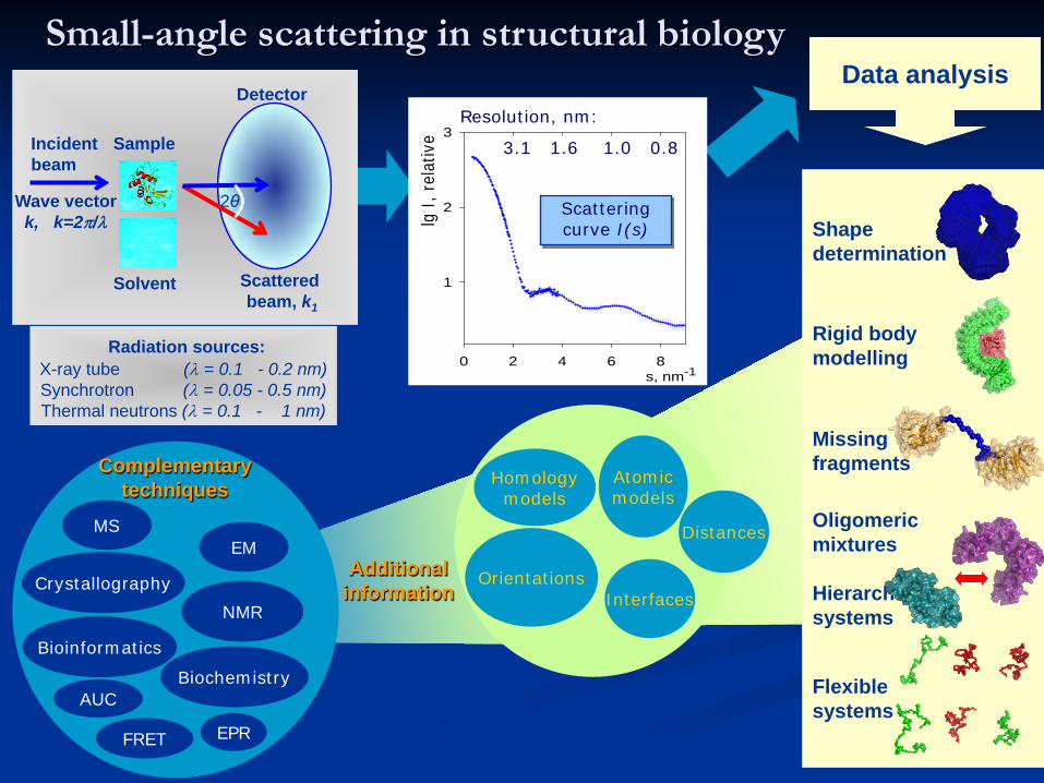
Complementary techniques

AUC

Oligomeric mixtures

Hierarchicalsystems

Shape determination

Flexible systems

Missing fragments

Rigid body modelling

Data analysis

Radiation sources:X-ray tube (λ = 0.1 - 0.2 nm)Synchrotron (λ = 0.05 - 0.5 nm)Thermal neutrons (λ = 0.1 - 1 nm)

Homologymodels

Atomicmodels

OrientationsInterfaces

Additional information

2θ

Sample

Solvent

Incident beam

Wave vector k, k=2π/λ

Detector

Scatteredbeam, k1

EPR

Small-angle scattering in structural biology

s, nm-10 2 4 6 8

lg I,

rela

tive

1

2

3

Scattering curve I(s)

Resolution, nm:

3.1 1.6 1.0 0.8

MS Distances

Major problem for biologists using SAS

• In the past, many biologists didnot believe that SAS yields more than the radius of gyration• Now, an immensely grownnumber of users are attracted by new possibilities of SAS and they want rapid answers to more and more complicated Questions• The users often have toperform numerous cumbersome actions during the experiment and data analysis, to become each of the Answers

Now we shall go through the major steps required on the way

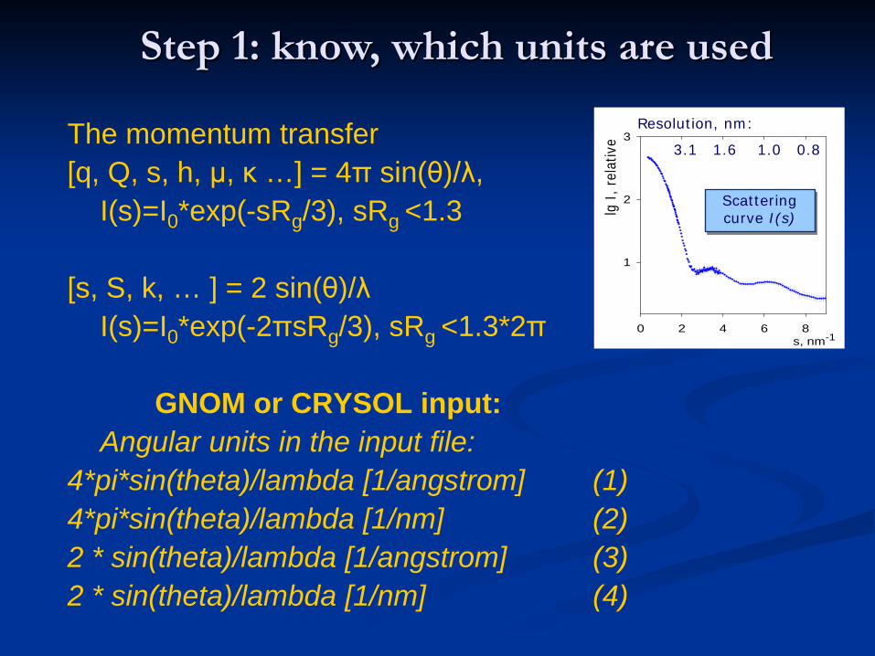
Step 1: know, which units are used

The momentum transfer[q, Q, s, h, μ, κ …] = 4π sin(θ)/λ,

I(s)=I0*exp(-sRg/3), sRg <1.3

[s, S, k, … ] = 2 sin(θ)/λI(s)=I0*exp(-2πsRg/3), sRg <1.3*2π

GNOM or CRYSOL input:Angular units in the input file:

4*pi*sin(theta)/lambda [1/angstrom] (1)4*pi*sin(theta)/lambda [1/nm] (2)2 * sin(theta)/lambda [1/angstrom] (3)2 * sin(theta)/lambda [1/nm] (4)

s, nm-10 2 4 6 8

lg I,

rela

tive

1

2

3

Scattering curve I(s)

Resolution, nm:

3.1 1.6 1.0 0.8

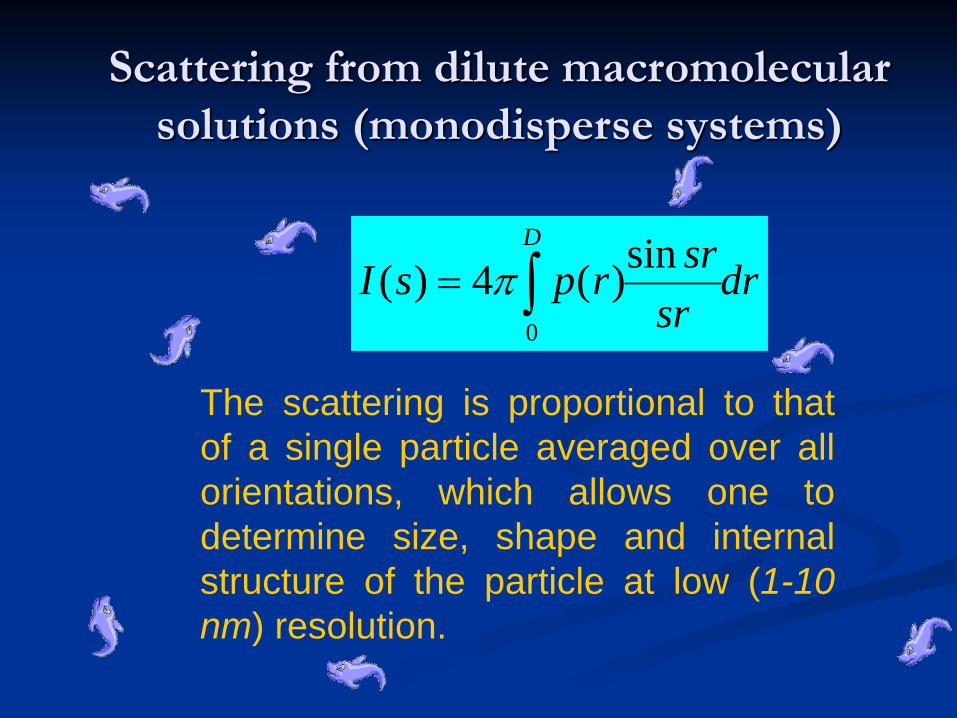
Scattering from dilute macromolecular solutions (monodisperse systems)

drsr

srrpsID

∫=0

sin)(4)( π

The scattering is proportional to thatof a single particle averaged over allorientations, which allows one todetermine size, shape and internalstructure of the particle at low (1-10nm) resolution.

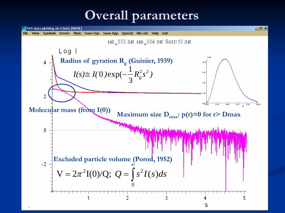
Overall parameters

)sR)I(I(s) g22

31exp(0 −≅

Radius of gyration Rg (Guinier, 1939)

Maximum size Dmax: p(r)=0 for r> Dmax

Excluded particle volume (Porod, 1952)

∫∞

==0

22 )( I(0)/Q;2V dssIsQπ

Molecular mass (from I(0))

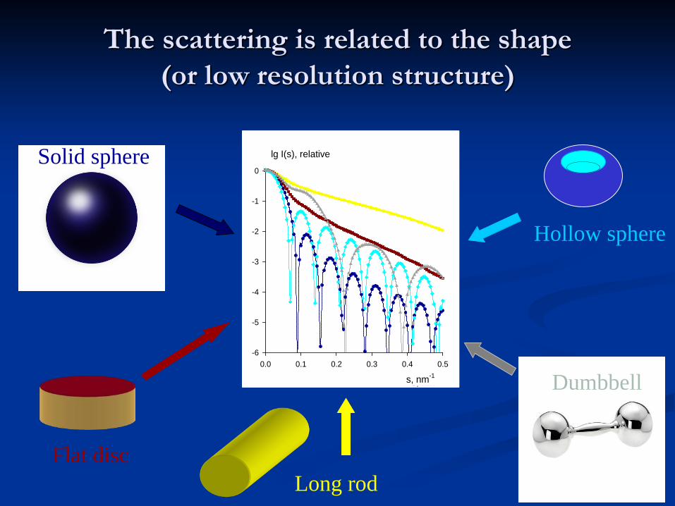
The scattering is related to the shape (or low resolution structure)

s, nm-10.0 0.1 0.2 0.3 0.4 0.5

lg I(s), relative

-6

-5

-4

-3

-2

-1

0Solid sphere

Long rodFlat disc

Hollow sphere

Dumbbells, nm-10.0 0.1 0.2 0.3 0.4 0.5

lg I(s), relative

-6

-5

-4

-3

-2

-1

0

s, nm-10.0 0.1 0.2 0.3 0.4 0.5

lg I(s), relative

-6

-5

-4

-3

-2

-1

0

s, nm-10.0 0.1 0.2 0.3 0.4 0.5

lg I(s), relative

-6

-5

-4

-3

-2

-1

0

s, nm-10.0 0.1 0.2 0.3 0.4 0.5

lg I(s), relative

-6

-5

-4

-3

-2

-1

0

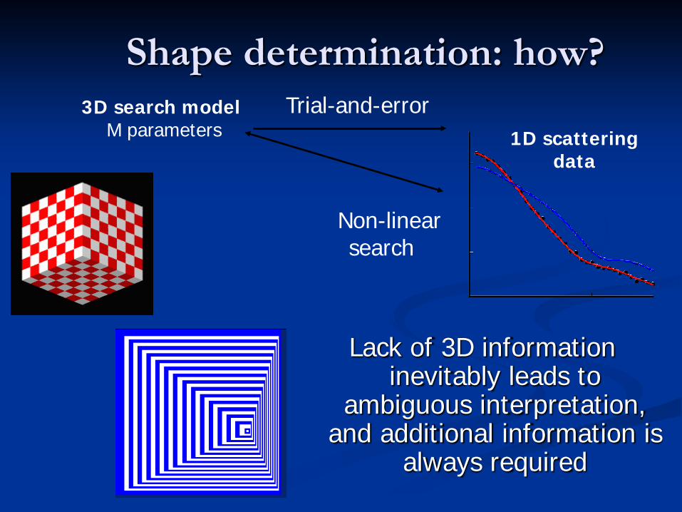
Shape determination: how?

Lack of 3D information inevitably leads to

ambiguous interpretation, and additional information is

always required

3D search modelM parameters

Non-linear search

1D scattering data

Trial-and-error

Ab initio methods

Advanced methods of SAS data analysis employ spherical harmonics (Stuhrmann, 1970) instead of Fourier

transformations

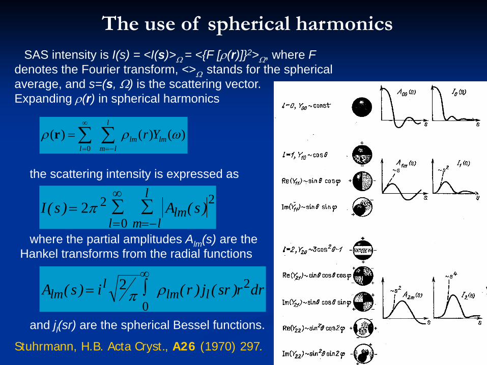
The use of spherical harmonicsSAS intensity is I(s) = <I(s)>Ω = <F [ρ(r)]2>Ω, where F

denotes the Fourier transform, <>Ω stands for the spherical average, and s=(s, Ω) is the scattering vector. Expanding ρ(r) in spherical harmonics

)()()(0

ωρρ lmlm

l

lmlYr∑∑

−=

∞

=

=r

the scattering intensity is expressed as

I s A sl m l

llm( ) ( )=

=

∞

=−∑ ∑2 2

0

2π

where the partial amplitudes Alm(s) are the Hankel transforms from the radial functions

A s i r j sr r drlml

lm l( ) ( ) ( )=∞∫20

2π ρ

and jl(sr) are the spherical Bessel functions.

Stuhrmann, H.B. Acta Cryst., A26 (1970) 297.

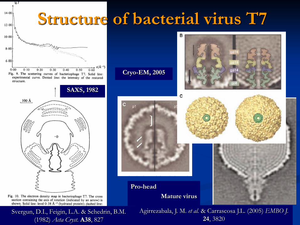
Structure of bacterial virus T7

Svergun, D.I., Feigin, L.A. & Schedrin, B.M. (1982) Acta Cryst. A38, 827

Agirrezabala, J. M. et al. & Carrascosa J.L. (2005) EMBO J.24, 3820

SAXS, 1982

Cryo-EM, 2005

Pro-headMature virus

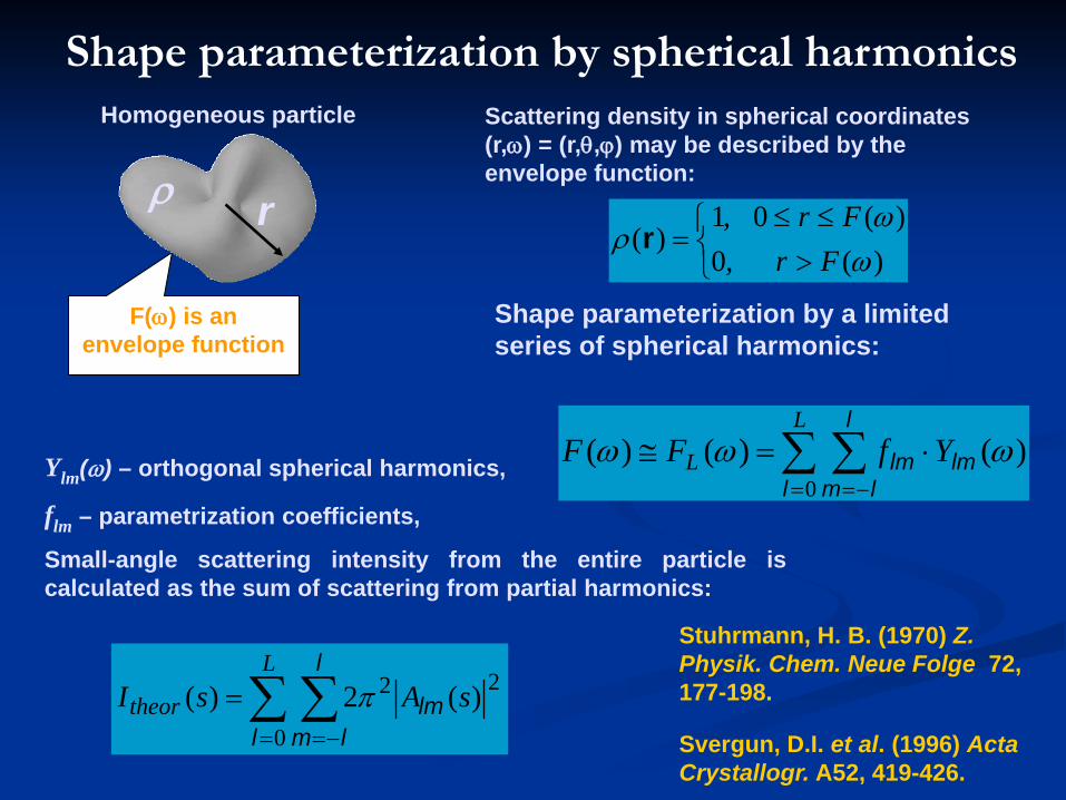
Ylm(ω) – orthogonal spherical harmonics,

flm – parametrization coefficients,

Small-angle scattering intensity from the entire particle iscalculated as the sum of scattering from partial harmonics:

∑ ∑= −=

⋅=≅L

L YfFF0

)()()(l

l

lmlmlm ωωω

Shape parameterization by spherical harmonicsHomogeneous particle Scattering density in spherical coordinates

(r,ω) = (r,θ,ϕ) may be described by the envelope function:

)()(0

,0,1

)(ωω

ρFr

Fr>≤≤

=r

Shape parameterization by a limited series of spherical harmonics:

∑ ∑= −=

=L

theor sAsI0

22 )(2)(l

l

lmlmπ

Stuhrmann, H. B. (1970) Z. Physik. Chem. Neue Folge 72, 177-198.

Svergun, D.I. et al. (1996) Acta Crystallogr. A52, 419-426.

F(ω) is an envelope function

rρ

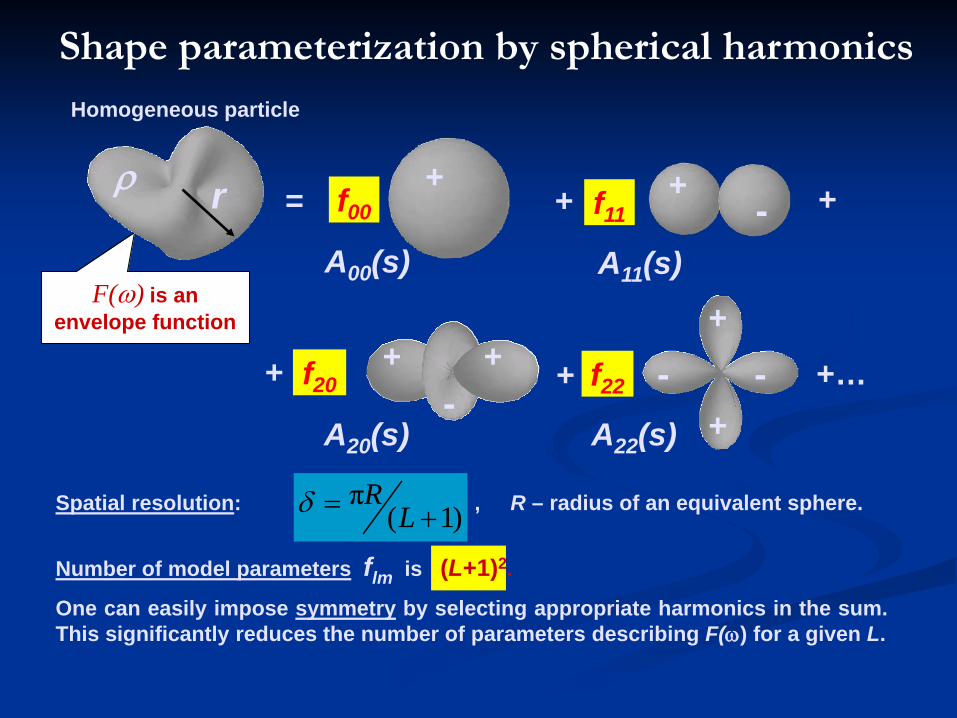
Homogeneous particle

f00

A00(s)

=+

f11+ +

A11(s)

+-

f20+

A20(s)

+-

+ f22+

A22(s) +--

++…

Spatial resolution: , R – radius of an equivalent sphere.

Number of model parameters flm is (L+1)2.

One can easily impose symmetry by selecting appropriate harmonics in the sum.This significantly reduces the number of parameters describing F(ω) for a given L.

)1(π

+= LRδ

F(ω) is an envelope function

rρ

Shape parameterization by spherical harmonics

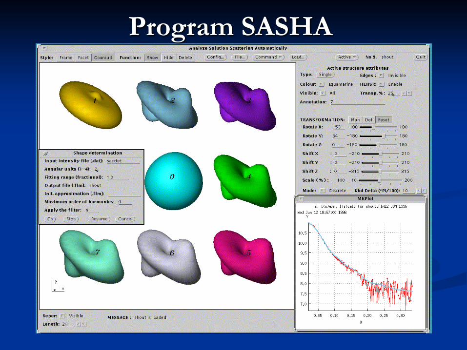
Program SASHA

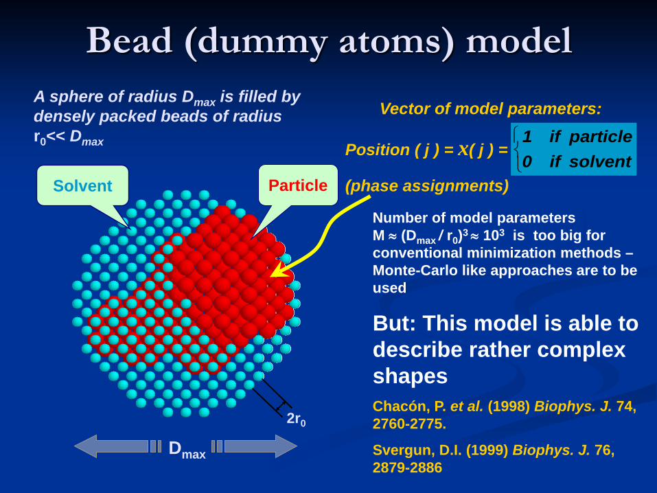
Vector of model parameters:

Position ( j ) = x( j ) =

(phase assignments)

Number of model parameters M ≈ (Dmax / r0)3 ≈ 103 is too big for conventional minimization methods –Monte-Carlo like approaches are to be used

But: This model is able to describe rather complex shapesChacón, P. et al. (1998) Biophys. J. 74, 2760-2775.

Svergun, D.I. (1999) Biophys. J. 76, 2879-2886

Solvent Particle

2r0

A sphere of radius Dmax is filled by densely packed beads of radiusr0<< Dmax

Dmax

solventif0particleif1

Bead (dummy atoms) model

Finding a global minimumPure Monte Carlo runs in a danger to be trapped into a

local minimum

Solution: use a global minimization method like simulated annealing or genetic algorithm

Local and global search on the Great Wall

Local search always goes to a better point and can thus be trapped in a local minimumPure Monte-Carlo search always goes to the closest local minimum (nature: rapid quenching and vitreous ice formation)To get out of local minima, global search must be able to (sometimes) go to a worse pointSlower annealing allows to search for a global minimum (nature: normal, e.g. slow freezing of water and ice formation)

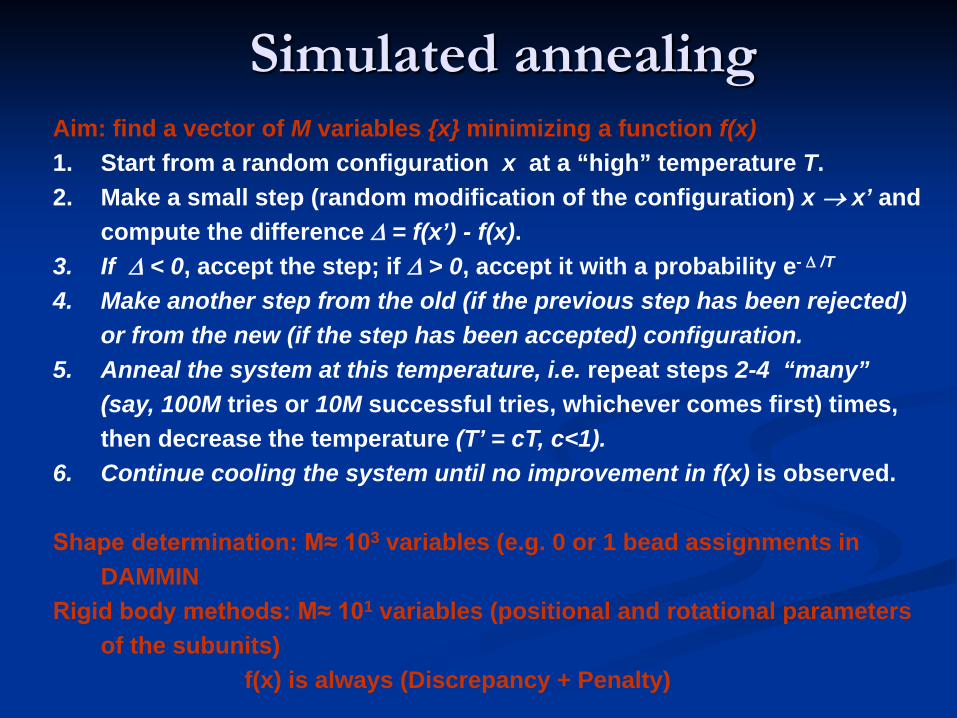
Aim: find a vector of M variables x minimizing a function f(x)1. Start from a random configuration x at a “high” temperature T.2. Make a small step (random modification of the configuration) x → x’ and

compute the difference ∆ = f(x’) - f(x).3. If ∆ < 0, accept the step; if ∆ > 0, accept it with a probability e- ∆ /T

4. Make another step from the old (if the previous step has been rejected)or from the new (if the step has been accepted) configuration.

5. Anneal the system at this temperature, i.e. repeat steps 2-4 “many”(say, 100M tries or 10M successful tries, whichever comes first) times,then decrease the temperature (T’ = cT, c<1).

6. Continue cooling the system until no improvement in f(x) is observed.

Shape determination: M≈ 103 variables (e.g. 0 or 1 bead assignments in DAMMIN

Rigid body methods: M≈ 101 variables (positional and rotational parameters of the subunits)

f(x) is always (Discrepancy + Penalty)

Simulated annealing

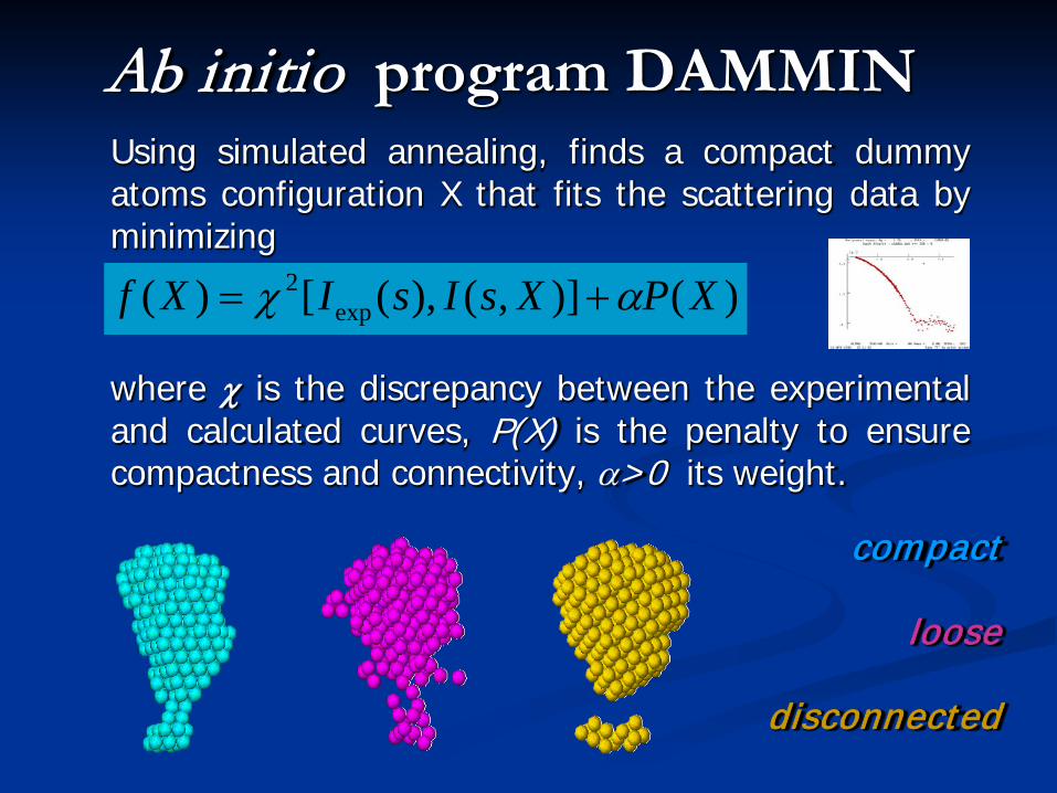
Ab initio program DAMMINUsing simulated annealing, finds a compact dummyatoms configuration X that fits the scattering data byminimizing

where χ is the discrepancy between the experimentaland calculated curves, P(X) is the penalty to ensurecompactness and connectivity, α>0 its weight.

)()],(),([)( exp2 XPXsIsIXf αχ +=

compact

loose

disconnected

Why/how do ab initio methods work

The 3D model is required not only to fit the data but also to fulfill (often stringent) physical and/or biochemical constrains

Why/how do ab initio methods work

The 3D model is required not only to fit the data but also to fulfill (often stringent) physical and/or biochemical constrains

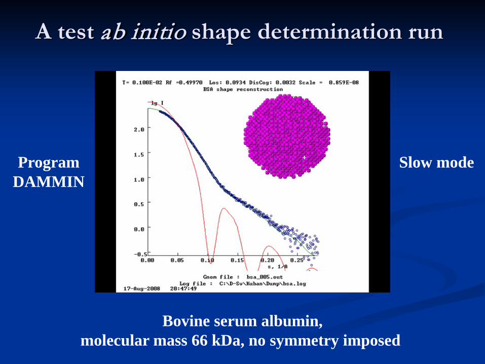
A test ab initio shape determination run

Bovine serum albumin,molecular mass 66 kDa, no symmetry imposed

ProgramDAMMIN

Slow mode

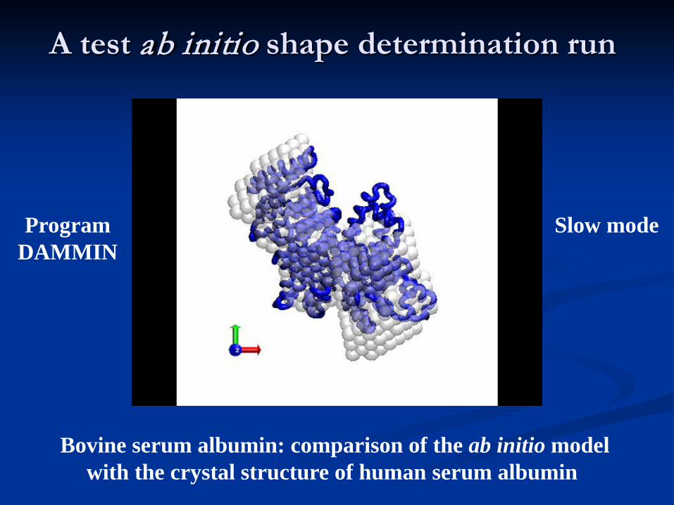
A test ab initio shape determination run

ProgramDAMMIN

Slow mode

Bovine serum albumin: comparison of the ab initio model with the crystal structure of human serum albumin

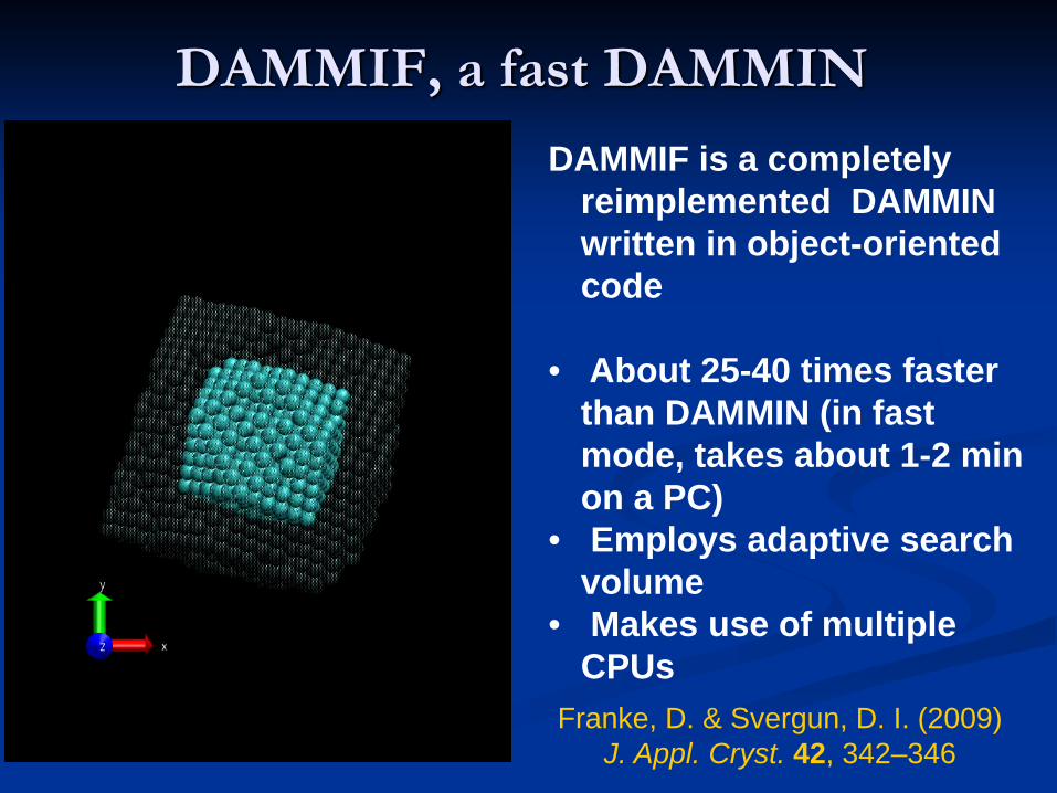
DAMMIF, a fast DAMMINDAMMIF is a completely

reimplemented DAMMIN written in object-oriented code

• About 25-40 times fasterthan DAMMIN (in fast mode, takes about 1-2 min on a PC)

• Employs adaptive searchvolume

• Makes use of multipleCPUs

Franke, D. & Svergun, D. I. (2009)J. Appl. Cryst. 42, 342–346

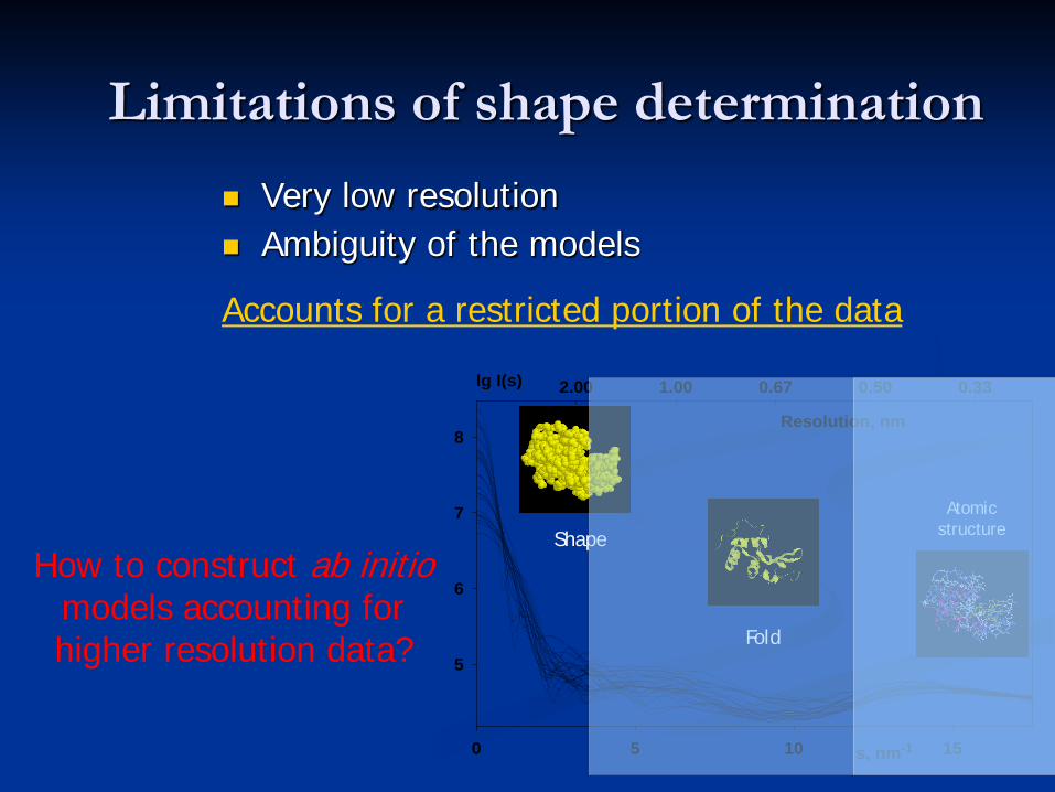
Limitations of shape determination Very low resolution Ambiguity of the models

s, nm-10 5 10 15

lg I(s)

5

6

7

8Resolution, nm

2.00 1.00 0.67 0.50 0.33

Shape

Fold

Atomic structure

How to construct ab initiomodels accounting for higher resolution data?

Accounts for a restricted portion of the data

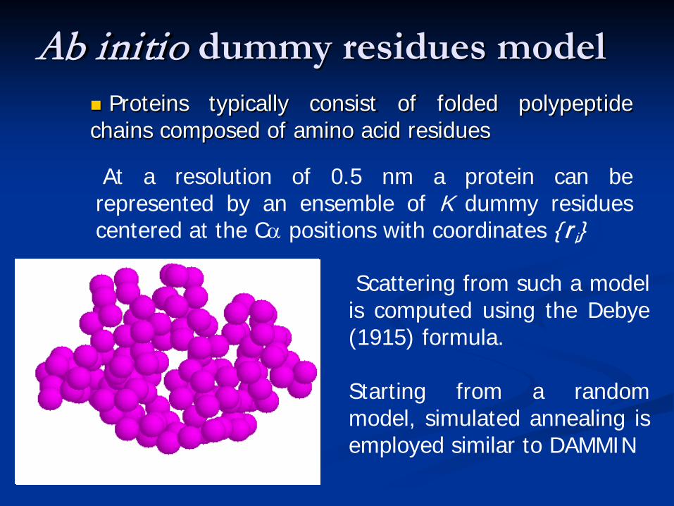
Ab initio dummy residues model Proteins typically consist of folded polypeptidechains composed of amino acid residues

Scattering from such a modelis computed using the Debye(1915) formula.

Starting from a randommodel, simulated annealing isemployed similar to DAMMIN

At a resolution of 0.5 nm a protein can berepresented by an ensemble of K dummy residuescentered at the Cα positions with coordinates ri

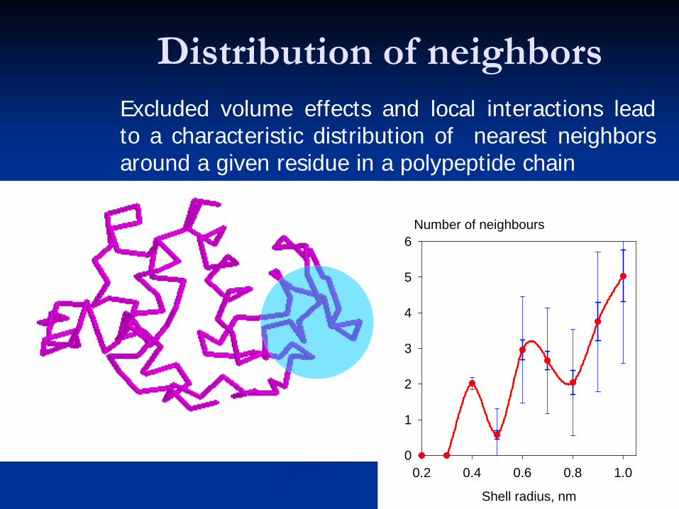
Distribution of neighborsExcluded volume effects and local interactions leadto a characteristic distribution of nearest neighborsaround a given residue in a polypeptide chain

Shell radius, nm

0.2 0.4 0.6 0.8 1.0

Number of neighbours

0

1

2

3

4

5

6

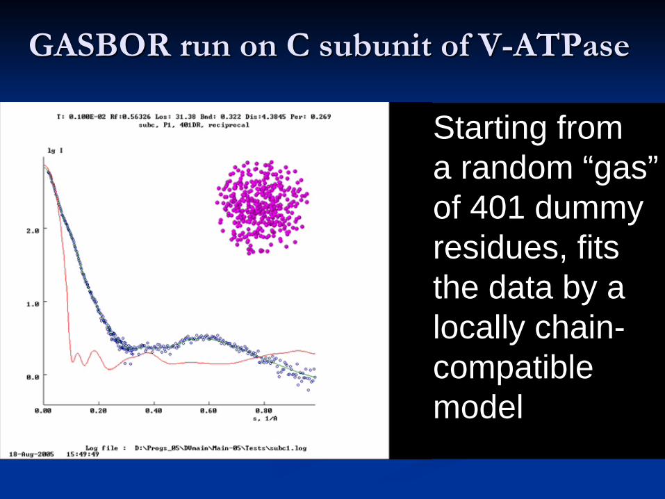
GASBOR run on C subunit of V-ATPase

Starting from a random “gas” of 401 dummy residues, fits the data by a locally chain-compatible model

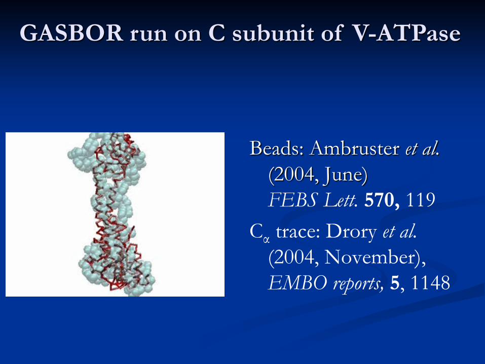
Beads: Ambruster et al.(2004, June) FEBS Lett. 570, 119

Cα trace: Drory et al. (2004, November), EMBO reports, 5, 1148

GASBOR run on C subunit of V-ATPase

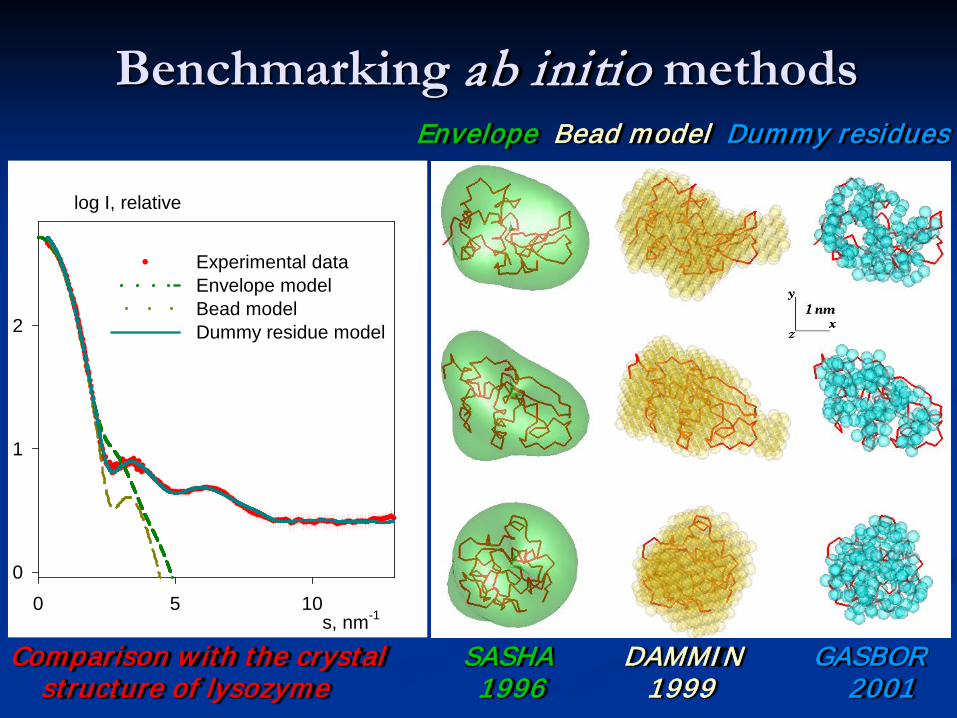
Benchmarking ab initio methods

s, nm-10 5 10

log I, relative

0

1

2

Experimental dataEnvelope modelBead model Dummy residue model

Comparison w ith the crystal SASHA DAMMIN GASBOR structure of lysozyme 1996 1999 2001

Envelope Bead model Dummy residues

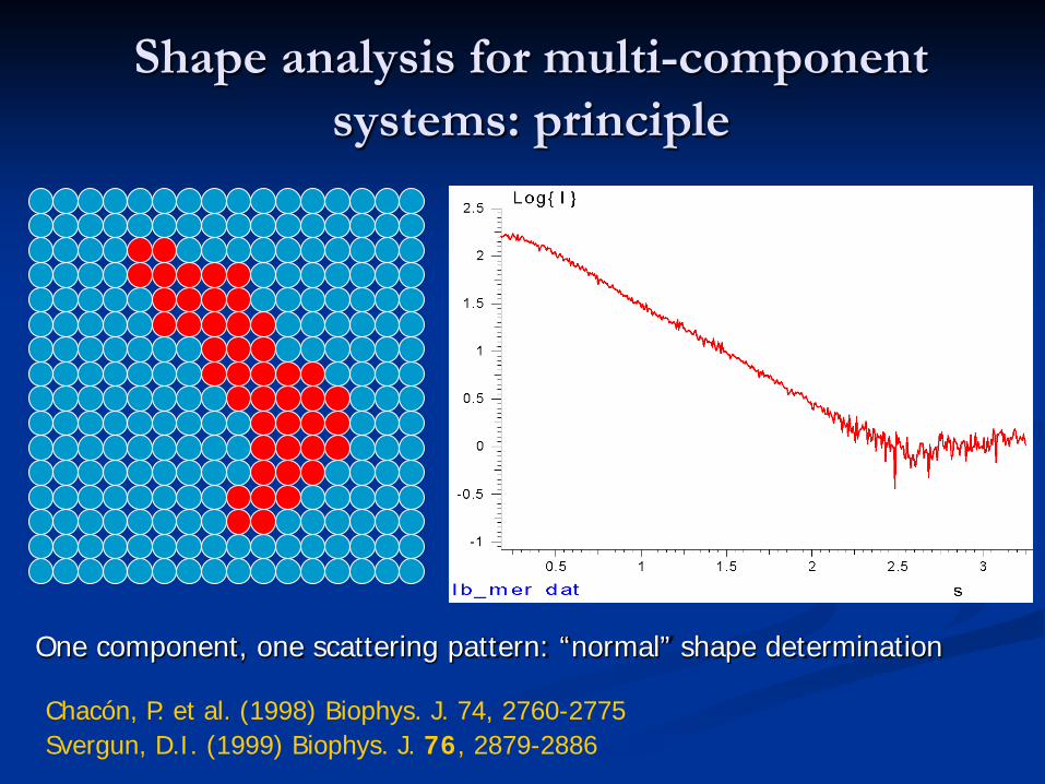
Shape analysis for multi-component systems: principle

One component, one scattering pattern: “normal” shape determination

Chacón, P. et al. (1998) Biophys. J. 74, 2760-2775Svergun, D.I. (1999) Biophys. J. 76, 2879-2886

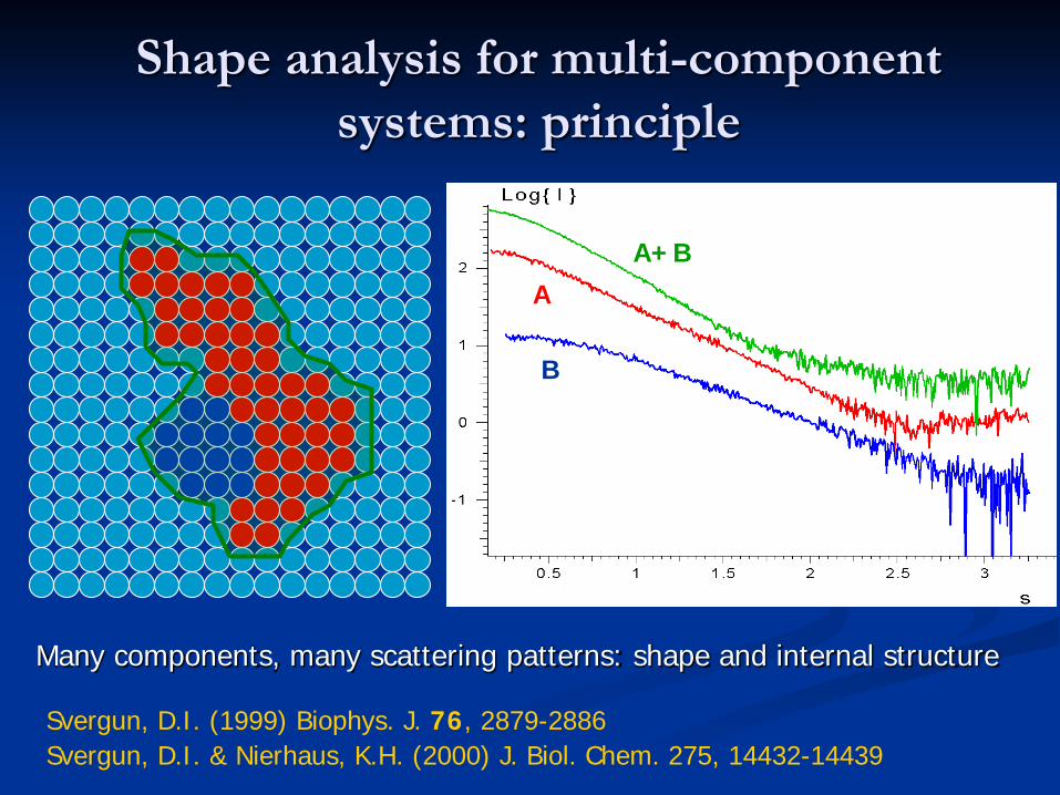
Shape analysis for multi-component systems: principle

Many components, many scattering patterns: shape and internal structure

Svergun, D.I. (1999) Biophys. J. 76, 2879-2886Svergun, D.I. & Nierhaus, K.H. (2000) J. Biol. Chem. 275, 14432-14439

A+BA

B

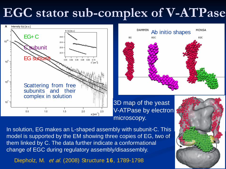
EGC stator sub-complex of V-ATPase

Diepholz, M. et al. (2008) Structure 16, 1789-1798

In solution, EG makes an L-shaped assembly with subunit-C. This model is supported by the EM showing three copies of EG, two of them linked by C. The data further indicate a conformational change of EGC during regulatory assembly/disassembly.

EG+C

C subunit

EG subunit

Scattering from freesubunits and theircomplex in solution

3D map of the yeast V-ATPase by electron microscopy.

Ab initio shapes

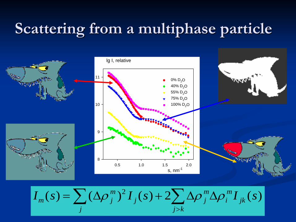
Scattering from a multiphase particle

s, nm-10.5 1.0 1.5 2.0

lg I, relative

8

9

10

11 0% D2O40% D2O55% D2O75% D2O100% D2O

∑∑>

∆∆+∆=kj

jkmi

mj

jj

mjm sIsIsI )(2)()()( 2 ρρρ

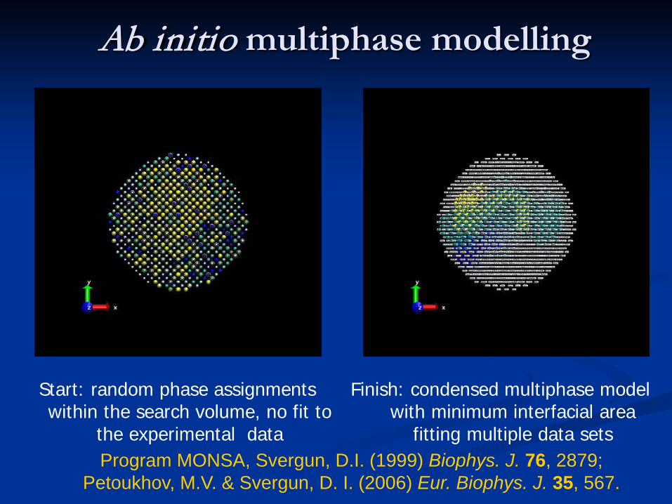
Ab initio multiphase modelling

Start: random phase assignments within the search volume, no fit to

the experimental data

Finish: condensed multiphase model with minimum interfacial area

fitting multiple data setsProgram MONSA, Svergun, D.I. (1999) Biophys. J. 76, 2879;

Petoukhov, M.V. & Svergun, D. I. (2006) Eur. Biophys. J. 35, 567.

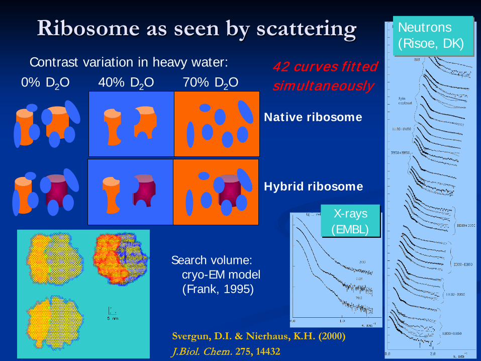
Ribosome as seen by scattering

X-rays(EMBL)

Neutrons(Risoe, DK)

Svergun, D.I. & Nierhaus, K.H. (2000) J.Biol. Chem. 275, 14432

42 curves fittedsimultaneously

Search volume: cryo-EM model (Frank, 1995)

Contrast variation in heavy water:0% D2O 40% D2O 70% D2O

Native ribosome

Hybrid ribosome

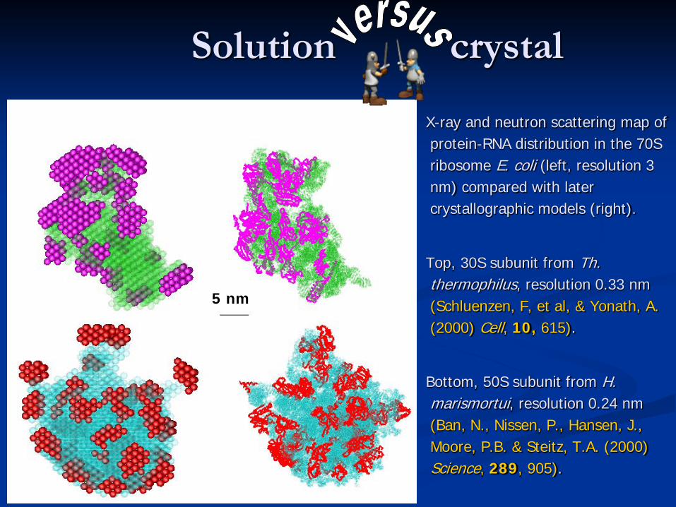
Solution crystal

X-ray and neutron scattering map of protein-RNA distribution in the 70S ribosome E. coli (left, resolution 3 nm) compared with later crystallographic models (right).

Top, 30S subunit from Th. thermophilus, resolution 0.33 nm (Schluenzen, F, et al, & Yonath, A. (2000) Cell, 10, 615).

Bottom, 50S subunit from H. marismortui, resolution 0.24 nm (Ban, N., Nissen, P., Hansen, J., Moore, P.B. & Steitz, T.A. (2000) Science, 289, 905).

5 nm

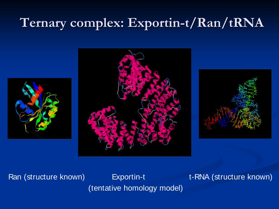
Ternary complex: Exportin-t/Ran/tRNA

Ran (structure known) Exportin-t t-RNA (structure known)(tentative homology model)

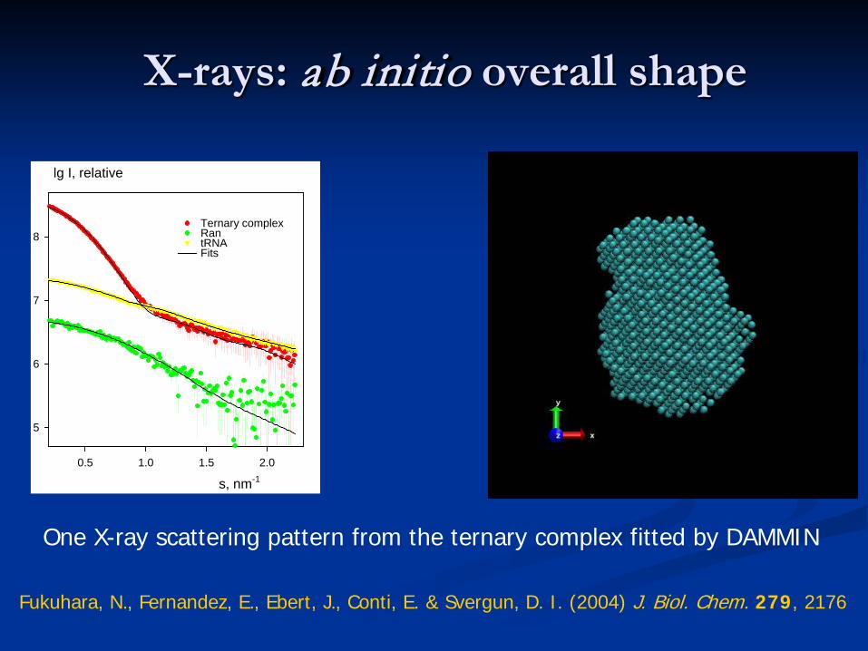
X-rays: ab initio overall shape

s, nm-1

0.5 1.0 1.5 2.0

lg I, relative

5

6

7

8Ternary complexRantRNAFits

One X-ray scattering pattern from the ternary complex fitted by DAMMIN

Fukuhara, N., Fernandez, E., Ebert, J., Conti, E. & Svergun, D. I. (2004) J. Biol. Chem. 279, 2176

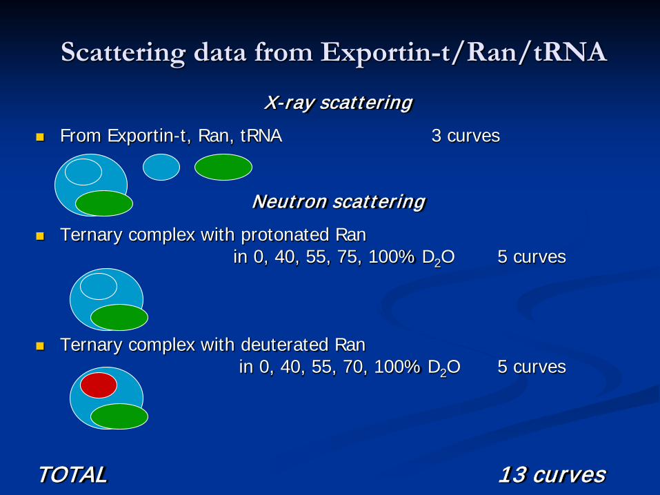
Scattering data from Exportin-t/Ran/tRNA

X-ray scattering From Exportin-t, Ran, tRNA 3 curves

Neutron scattering Ternary complex with protonated Ran

in 0, 40, 55, 75, 100% D2O 5 curves

Ternary complex with deuterated Ranin 0, 40, 55, 70, 100% D2O 5 curves

TOTAL 13 curves

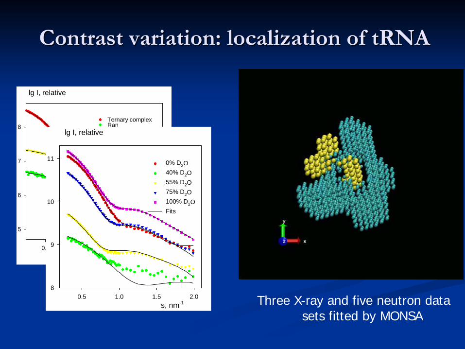
Contrast variation: localization of tRNA

s, nm-1

0.5 1.0 1.5 2.0

lg I, relative

5

6

7

8Ternary complexRantRNAFits

s, nm-10.5 1.0 1.5 2.0

lg I, relative

8

9

10

11 0% D2O40% D2O55% D2O75% D2O100% D2OFits

Three X-ray and five neutron data sets fitted by MONSA

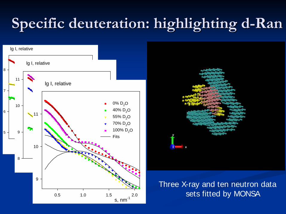
Specific deuteration: highlighting d-Ran

s, nm-1

0.5 1.0 1.5 2.0

lg I, relative

5

6

7

8Ternary complexRantRNAFits

s, nm-10.5 1.0 1.5 2.0

lg I, relative

8

9

10

11 0% D2O40% D2O55% D2O75% D2O100% D2OFits

s, nm-10.5 1.0 1.5 2.0

lg I, relative

9

10

11

0% D2O40% D2O55% D2O70% D2O100% D2OFits

Three X-ray and ten neutron data sets fitted by MONSA

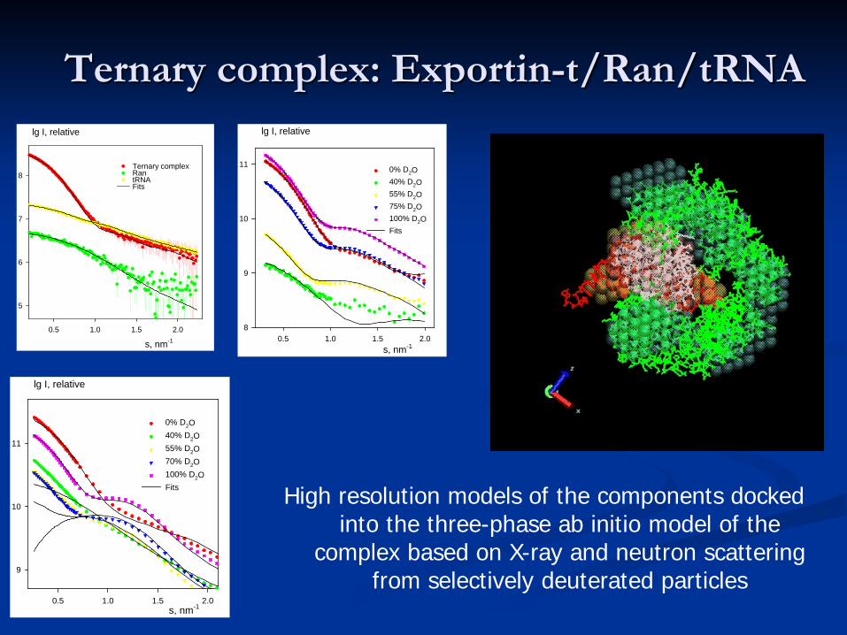
Ternary complex: Exportin-t/Ran/tRNA

s, nm-1

0.5 1.0 1.5 2.0

lg I, relative

5

6

7

8Ternary complexRantRNAFits

s, nm-10.5 1.0 1.5 2.0

lg I, relative

8

9

10

11 0% D2O40% D2O55% D2O75% D2O100% D2OFits

s, nm-10.5 1.0 1.5 2.0

lg I, relative

9

10

11

0% D2O40% D2O55% D2O70% D2O100% D2OFits High resolution models of the components docked

into the three-phase ab initio model of the complex based on X-ray and neutron scattering

from selectively deuterated particles

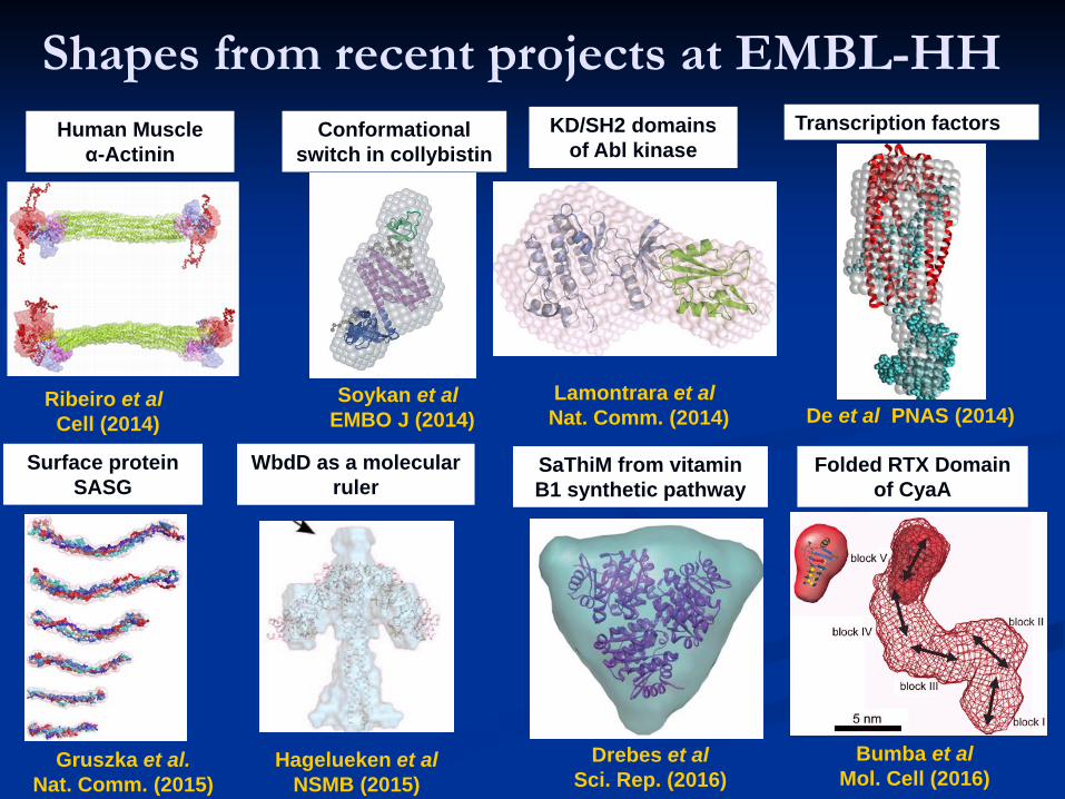
Shapes from recent projects at EMBL-HHKD/SH2 domains

of Abl kinase

Lamontrara et al Nat. Comm. (2014)

Ribeiro et al Cell (2014)

Human Muscle α-Actinin

WbdD as a molecular ruler

Hagelueken et al NSMB (2015)

Gruszka et al.Nat. Comm. (2015)

Surface protein SASG

Soykan et al EMBO J (2014)

Conformational switch in collybistin

SaThiM from vitamin B1 synthetic pathway

Drebes et al Sci. Rep. (2016)

Folded RTX Domain of CyaA

Bumba et al Mol. Cell (2016)

Transcription factors

De et al PNAS (2014)

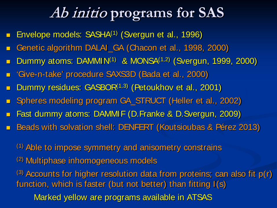
Ab initio programs for SAS Envelope models: SASHA(1) (Svergun et al., 1996) Genetic algorithm DALAI_GA (Chacon et al., 1998, 2000) Dummy atoms: DAMMIN(1) & MONSA(1,2) (Svergun, 1999, 2000) ‘Give-n-take’ procedure SAXS3D (Bada et al., 2000) Dummy residues: GASBOR(1,3) (Petoukhov et al., 2001) Spheres modeling program GA_STRUCT (Heller et al., 2002) Fast dummy atoms: DAMMIF (D.Franke & D.Svergun, 2009) Beads with solvation shell: DENFERT (Koutsioubas & Pérez 2013)

(1) Able to impose symmetry and anisometry constrains(2) Multiphase inhomogeneous models (3) Accounts for higher resolution data from proteins; can also fit p(r) function, which is faster (but not better) than fitting I(s)

Marked yellow are programs available in ATSAS

Some words of caution

Or Always remember about ambiguity!

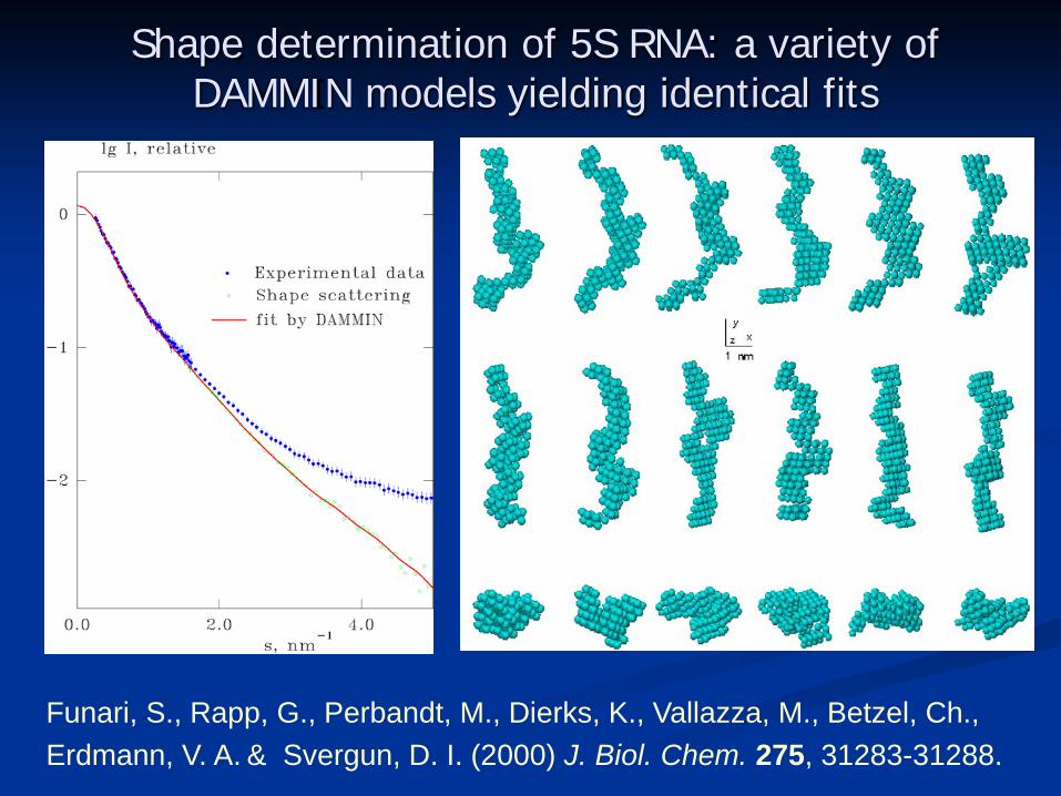
Shape determination of 5S RNA: a variety of DAMMIN models yielding identical fits

Funari, S., Rapp, G., Perbandt, M., Dierks, K., Vallazza, M., Betzel, Ch., Erdmann, V. A. & Svergun, D. I. (2000) J. Biol. Chem. 275, 31283-31288.

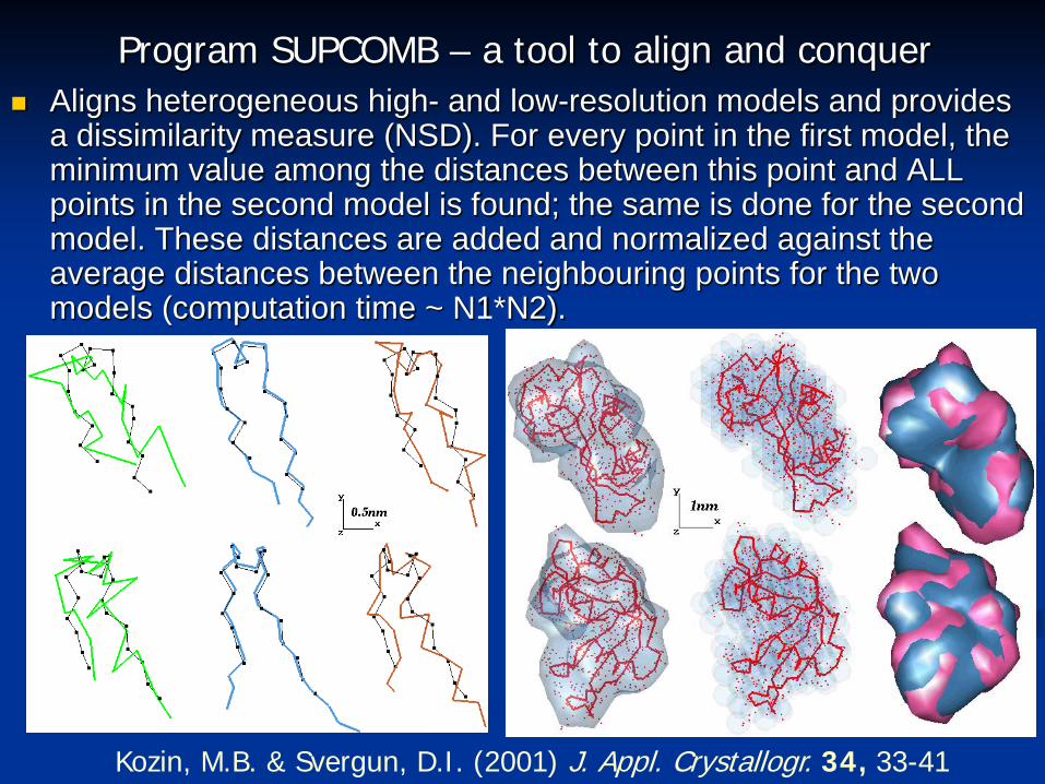
Kozin, M.B. & Svergun, D.I. (2001) J. Appl. Crystallogr. 34, 33-41

Program SUPCOMB – a tool to align and conquer Aligns heterogeneous high- and low-resolution models and provides

a dissimilarity measure (NSD). For every point in the first model, the minimum value among the distances between this point and ALL points in the second model is found; the same is done for the second model. These distances are added and normalized against the average distances between the neighbouring points for the two models (computation time ~ N1*N2).

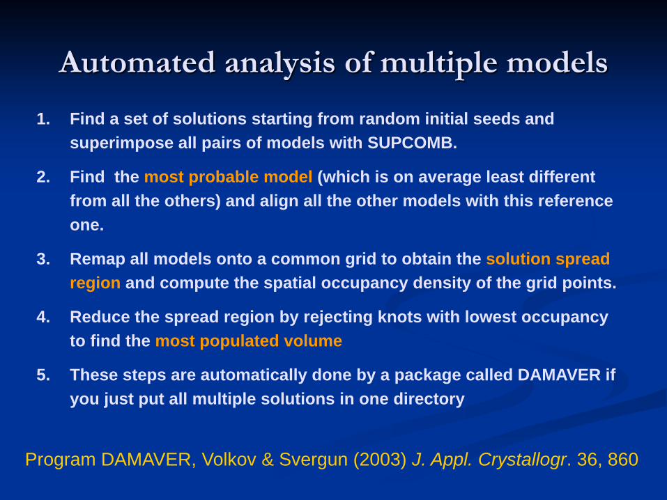
1. Find a set of solutions starting from random initial seeds and superimpose all pairs of models with SUPCOMB.

2. Find the most probable model (which is on average least different from all the others) and align all the other models with this reference one.

3. Remap all models onto a common grid to obtain the solution spread region and compute the spatial occupancy density of the grid points.

4. Reduce the spread region by rejecting knots with lowest occupancy to find the most populated volume

5. These steps are automatically done by a package called DAMAVER if you just put all multiple solutions in one directory

Automated analysis of multiple models

Program DAMAVER, Volkov & Svergun (2003) J. Appl. Crystallogr. 36, 860

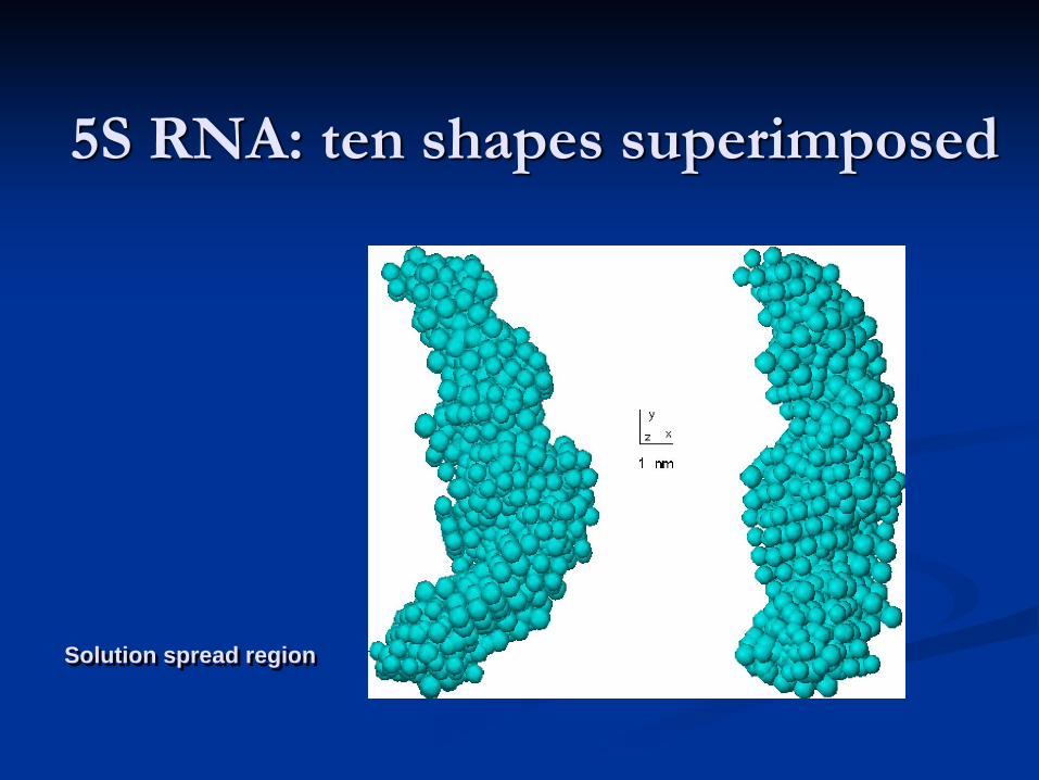
5S RNA: ten shapes superimposed

Solution spread region

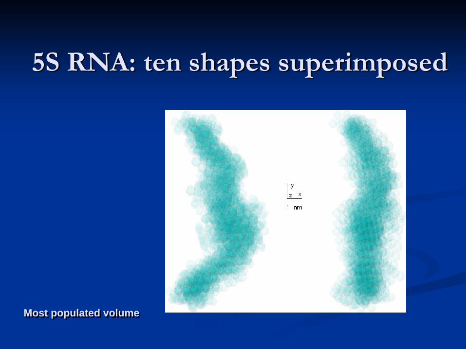
5S RNA: ten shapes superimposed

Most populated volume

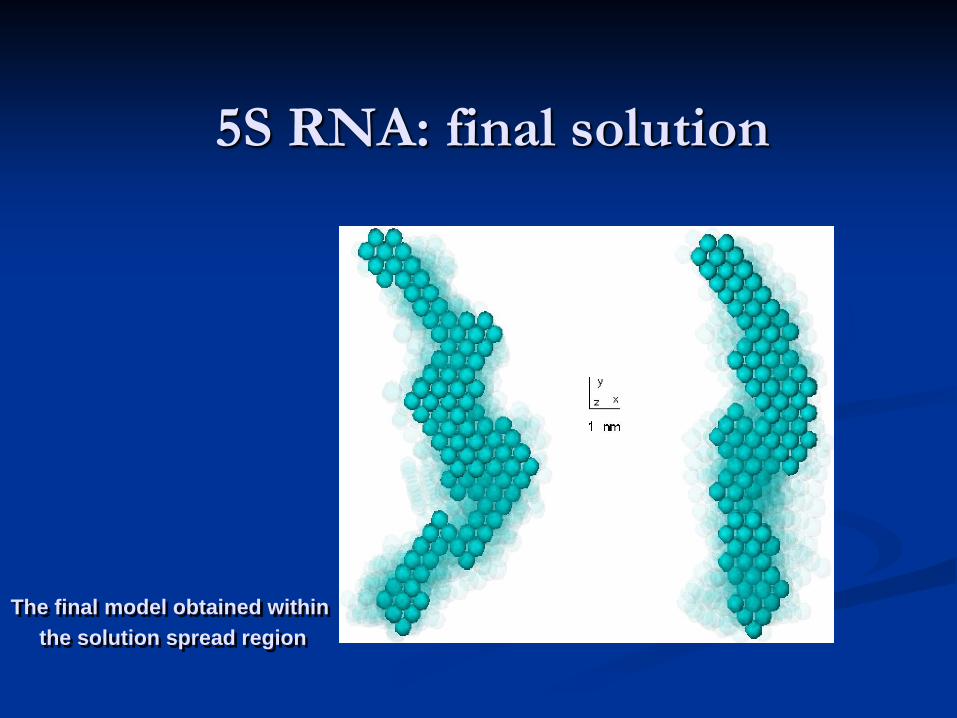
5S RNA: final solution

The final model obtained within the solution spread region

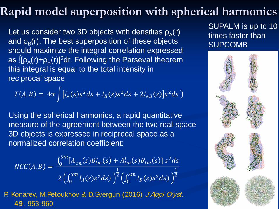
Rapid model superposition with spherical harmonics

Using the spherical harmonics, a rapid quantitative measure of the agreement between the two real-space 3D objects is expressed in reciprocal space as a normalized correlation coefficient:

P. Konarev, M.Petoukhov & D.Svergun (2016) J Appl Cryst. 49, 953-960

Let us consider two 3D objects with densities ρA(r) and ρB(r). The best superposition of these objects should maximize the integral correlation expressed as ∫[ρA(r)+ρB(r)]2dr. Following the Parseval theorem this integral is equal to the total intensity in reciprocal space

𝑇𝑇 𝐴𝐴,𝐵𝐵 = 4𝜋𝜋 𝐼𝐼𝐴𝐴 𝑠𝑠 𝑠𝑠2𝑑𝑑𝑠𝑠 + 𝐼𝐼𝐵𝐵 𝑠𝑠 𝑠𝑠2𝑑𝑑𝑠𝑠 + 2𝐼𝐼𝐴𝐴𝐵𝐵 𝑠𝑠 𝑠𝑠2𝑑𝑑𝑠𝑠

𝑁𝑁𝑁𝑁𝑁𝑁 𝐴𝐴,𝐵𝐵 =∫0𝑆𝑆𝑆𝑆[𝐴𝐴𝑙𝑙𝑆𝑆 𝑠𝑠 𝐵𝐵𝑙𝑙𝑆𝑆∗ 𝑠𝑠 + 𝐴𝐴𝑙𝑙𝑆𝑆∗ 𝑠𝑠 𝐵𝐵𝑙𝑙𝑆𝑆 𝑠𝑠 ] 𝑠𝑠2𝑑𝑑𝑠𝑠

2 ∫0𝑆𝑆𝑆𝑆 𝐼𝐼𝐴𝐴(𝑠𝑠)𝑠𝑠2𝑑𝑑𝑠𝑠)

12 ∫0

𝑆𝑆𝑆𝑆 𝐼𝐼𝐵𝐵(𝑠𝑠)𝑠𝑠2𝑑𝑑𝑠𝑠)12

SUPALM is up to 10 times faster than SUPCOMB

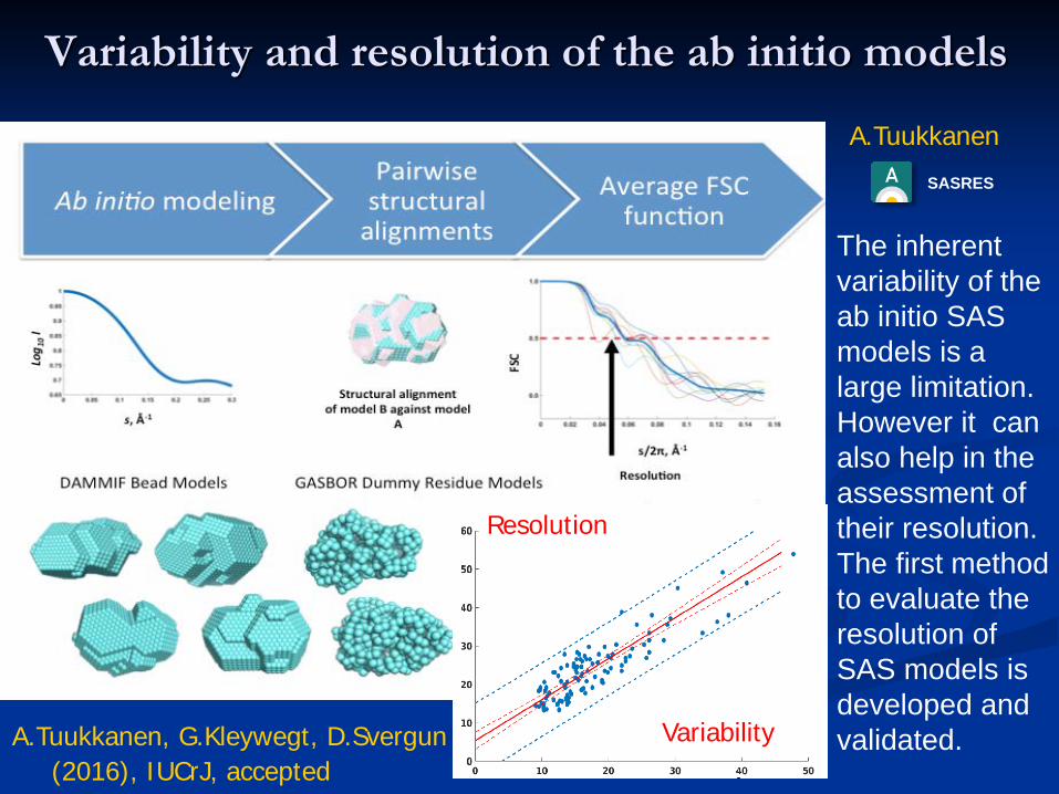
Variability and resolution of the ab initio models

The inherent variability of the ab initio SAS models is a large limitation. However it can also help in the assessment of their resolution. The first method to evaluate the resolution of SAS models is developed and validated.

A.TuukkanenSASRES

A.Tuukkanen, G.Kleywegt, D.Svergun(2016), IUCrJ, accepted

Resolution

Variability

0.0 0.2 0.4 0.6 0.8 1.0

10-4

10-3

10-2

10-1

100

s

I

data SASHA DAMMIN

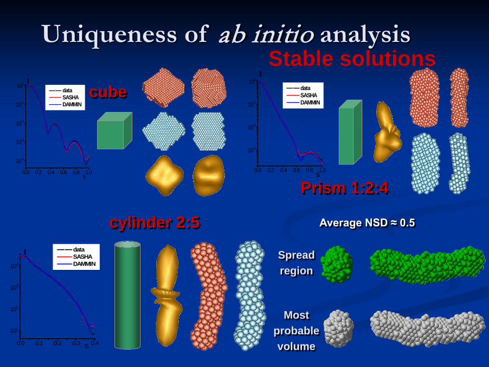
Stable solutions

0.0 0.2 0.4 0.6 0.8 1.0

10-3

10-2

10-1

100

s

I

data SASHA DAMMIN

0.0 0.1 0.2 0.3 0.4

101

102

103

104

s

I

data SASHA DAMMIN

cylinder 2:5

cube

Prism 1:2:4

Spread region

Most probable volume

Average NSD ≈ 0.5

Uniqueness of ab initio analysis

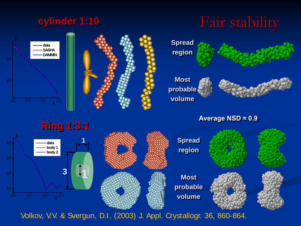
Fair stability

0.0 0.1 0.2 0.3

103

104

s

I

data SASHA DAMMIN

0.0 0.1 0.2 0.3

102

103

104

105

s

I

data body 1 body 2

3

1

1

cylinder 1:10

Ring 1:3:1

Spread region

Most probable volume

Spread region

Most probable volume

Average NSD ≈ 0.9

Volkov, V.V. & Svergun, D.I. (2003) J. Appl. Crystallogr. 36, 860-864.

0.0 0.1 0.2 0.3101

102

103

104

105

s

I

data SASHA DAMMIN

0.0 0.1 0.2 0.3

103

104

s

I

data SASHA DAMMIN

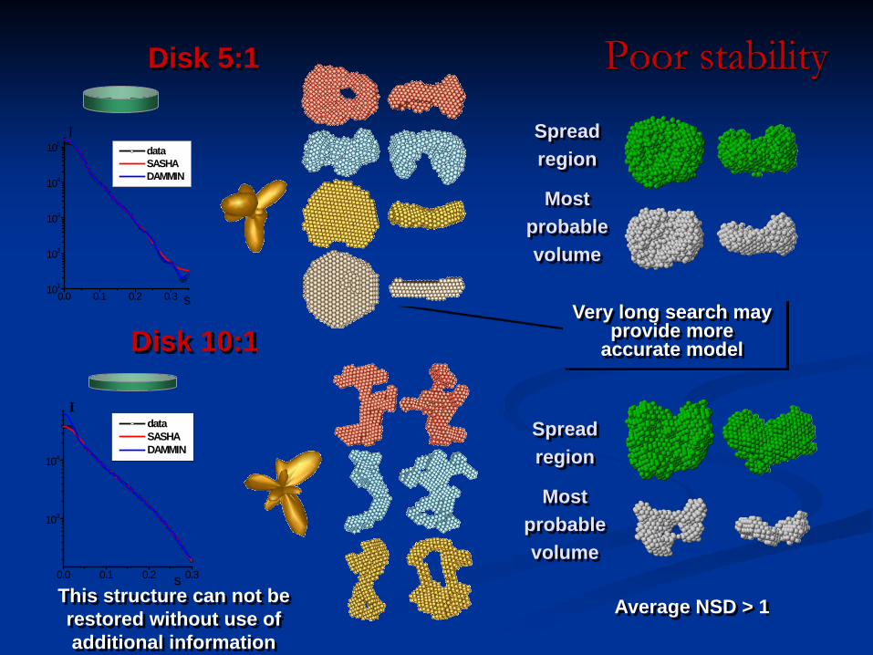
Poor stability

Spread region

Most probable volume

Spread region

Most probable volume

Disk 10:1

Disk 5:1

Very long search may provide more

accurate model

This structure can not be restored without use of additional information

Average NSD > 1

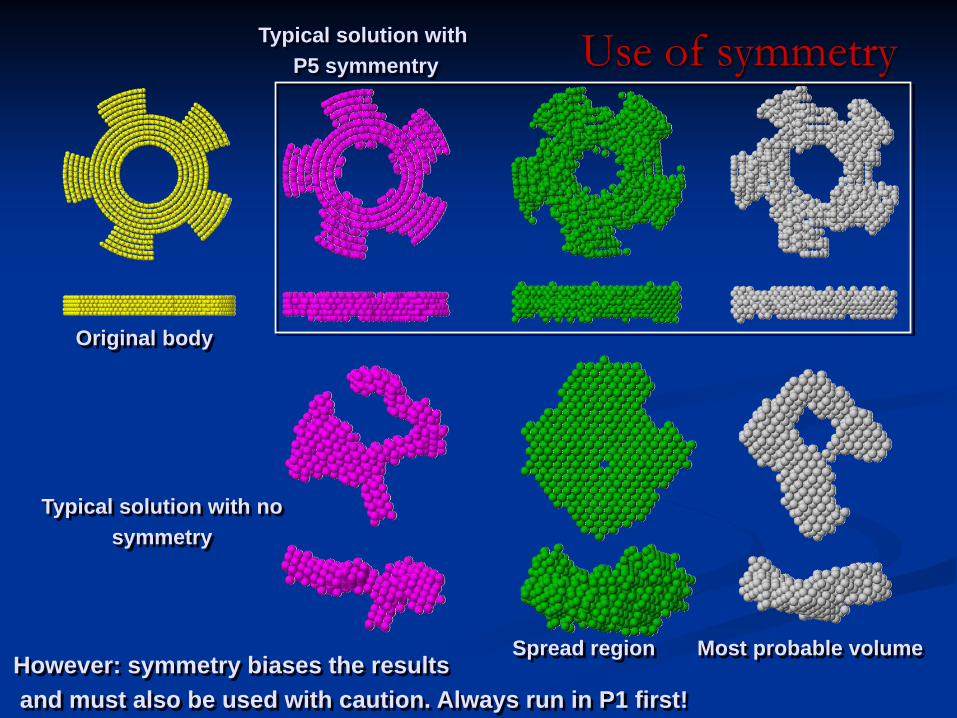
Use of symmetry

Original body

Typical solution with P5 symmentry

Typical solution with no symmetry

Spread region Most probable volumeHowever: symmetry biases the resultsand must also be used with caution. Always run in P1 first!

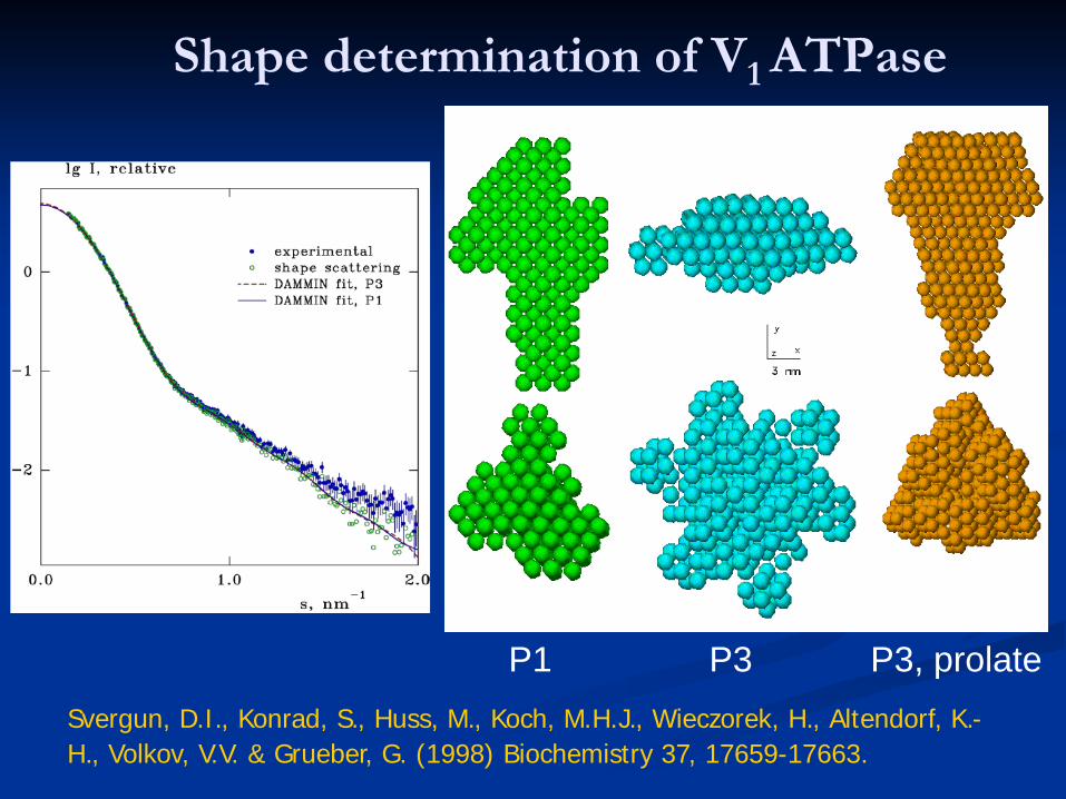
Shape determination of V1 ATPase

P1 P3 P3, prolateSvergun, D.I., Konrad, S., Huss, M., Koch, M.H.J., Wieczorek, H., Altendorf, K.-H., Volkov, V.V. & Grueber, G. (1998) Biochemistry 37, 17659-17663.

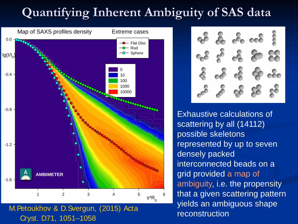
Quantifying Inherent Ambiguity of SAS data

Exhaustive calculations of scattering by all (14112) possible skeletons represented by up to seven densely packed interconnected beads on a grid provided a map of ambiguity, i.e. the propensity that a given scattering pattern yields an ambiguous shape reconstruction

Map of SAXS profiles density

s*Rg1 2 3 4 5 6

lg(I/I0)

-1.6

-1.2

-0.8

-0.4

0.0

010 100 1000 10000

Extreme cases

Flat DiscRodSphere

M.Petoukhov & D.Svergun, (2015) ActaCryst. D71, 1051–1058

AMBIMETER

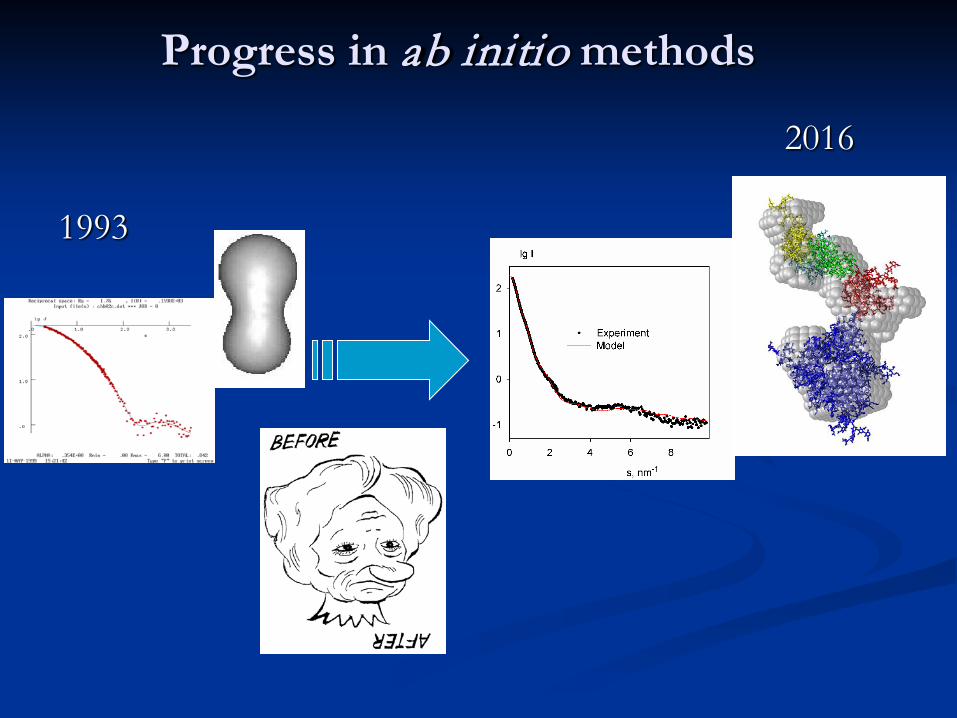
Progress in ab initio methods

2016

1993