A SYMBOL-BASED ALGORITHM FOR DECODING BAR CODES · The multiplier α lumps the conversion from...

SIAM J. IMAGING SCIENCES c© 20XX Society for Industrial and Applied MathematicsVol. 0, pp. 000-000

A SYMBOL-BASED ALGORITHM FOR DECODING BAR CODES∗

Mark A. Iwen†, Fadil Santosa‡§, and Rachel Ward¶

Abstract. We investigate the problem of decoding a bar code from a signal measured with a hand-held laser-based scanner. Rather than formulating the inverse problem as one of binary image reconstruction,we instead incorporate the symbology of the bar code into the reconstruction algorithm directly,and search for a sparse representation of the UPC bar code with respect to this known dictionary.Our approach significantly reduces the degrees of freedom in the problem, allowing for accuratereconstruction that is robust to noise and unknown parameters in the scanning device. We pro-pose a greedy reconstruction algorithm and provide robust reconstruction guarantees. Numericalexamples illustrate the insensitivity of our symbology-based reconstruction to both imprecise modelparameters and noise on the scanned measurements.

Key words. Bar code decoding, symbol-based method, deconvolution, parameter estimation, inverse problem.

AMS subject classifications. AAA-xxx-00

1. Introduction. This work concerns an approach for decoding bar code signals. While itis true that bar code scanning is essentially a solved problem in many domains, as evidenced byits prevalent use, there is still a need for more reliable decoding algorithms in situations wherethe signals are highly corrupted and the scanning takes place in less than ideal situations. Itis under these conditions that traditional bar code scanning algorithms often fail.

The problem of bar code decoding may be viewed as the deconvolution of a binary one-dimensional image involving unknown parameters in the blurring kernel that must be esti-mated from the signal [6]. Esedoglu [6] was the first to provide a mathematical analysis ofthe bar code decoding problem in this context, and he established the first uniqueness resultof its kind for this problem. He further showed that the blind deconvolution problem canbe formulated as a well-posed variational problem. An approximation, based on the Modica-Mortola energy [11], is the basis for the computational approach. The approach has recentlybeen given further analytical treatment in [7].

A recent work [2] addresses the case where the blurring is not very severe. Indeed theauthors were able to treat the signal as if it has not been blurred. They showed rigorouslythe variational framework can recover the true bar code image even if this parameter is notknown. A later paper [3] consider the case where blurring is large and its parameter valueknown. However, none of these papers deal rigorously with noise although their numerical

∗Submitted to SIIMS on DATE.†Mathematics Department, Duke University, Durham, NC 27708 ([email protected]). The research of

this author was supported in part by ONR N00014-07-1-0625 and NSF DMS DMS-0847388.§School of Mathematics, University of Minnesota, Minneapolis, MN 55455 ([email protected]). The re-

search of this author was supported in part by NSF DMS-0807856.¶Department of Mathematics, University of Texas at Austin, 2515 Speedway, Austin, TX, 78712

([email protected]). The research of this author was supported in part by the NSF Postdoctoral ResearchFellowship and the Donald D. Harrington Faculty Fellowship.

1

2 M. A. IWEN, F. SANTOSA, AND R. WARD

simulations included noise. For an analysis of the deblurring problem where the blur is largeand noise is present, the reader is referred to [7].

The approach presented in this work departs from the above image-based approaches. Wetreat the unknown as a finite-dimensional code and develop a model that relates the code tothe measured signal. We show that by exploiting the symbology – the language of the barcode – a bar code can be identified with a sparse representation in the symbology dictionary.We develop a recovery algorithm that fits the observed signal to a code from the symbologyin a greedy fashion, iterating in one pass from left to right. We prove that the algorithm cantolerate a significant level of blur and noise. We also verify insensitivity of the reconstructionto imprecise parameter estimation of the blurring function.

We were unable to find any previous symbol-based methods for bar code decoding inthe open literature. In a related approach [4], a genetic algorithm is utilized to representpopulations of candidate barcodes together with likely blurring and illumination parametersfrom the observed image data. Successive generations of candidate solutions are then spawnedfrom those best matching the input data until a stopping criterion is met. That work differsfrom the current article in that it uses a different decoding method and does not utilize therelationship between the structure of the barcode symbology and the blurring kernel.

We note that there is a symbol-based approach for super-resolving scanned images [1].However, that work is statistical in nature whereas the method we present is deterministic.Both this work and the super-resolution work are similar in spirit to lossless data compressionalgorithms known as ‘dictionary coding’ (see, e.g., [12]) which involve matching strings of textto strings contained in an encoding dictionary.

The outline of the paper is as follows. We start by developing a model for the scanningprocess. In Section 3, we study the properties of the UPC (Universal Product Code) barcode and provide a mathematical representation for the code. Section 4 develops the relationbetween the code and the measured signal. An algorithm for decoding bar code signals ispresented in Section 5. Section 6 is devoted to the analysis of the algorithm proposed. Resultsfrom numerical experiments are presented in Section 7, and a final section concludes the workwith a discussion.

2. A scanning model and associated inverse problem. A bar code is scanned by shininga narrow laser beam across the black-and-white bars at constant speed. The amount of lightreflected as the beam moves is recorded and can be viewed as a signal in time. Since the barcode consists of black and white segments, the reflected energy is large when the beam is onthe white part, and small when the beam is on the black part. The reflected light energy at agiven position is proportional to the integral of the product of the beam intensity, which canbe modeled as a Gaussian1, and the bar code image intensity (white is high intensity, blackis low). The recorded data are samples of the resulting continuous time signal.

Let us write the Gaussian beam intensity as a function of time:

g(t) = α1√2πσ

e−(t2/2σ2). (2.1)

1This Gaussian model has also been utilized in many previous treatments of the bar code decoding problem.See, e.g., [8] and references therein.

SYMBOL-BASED BAR CODE DECODING 3

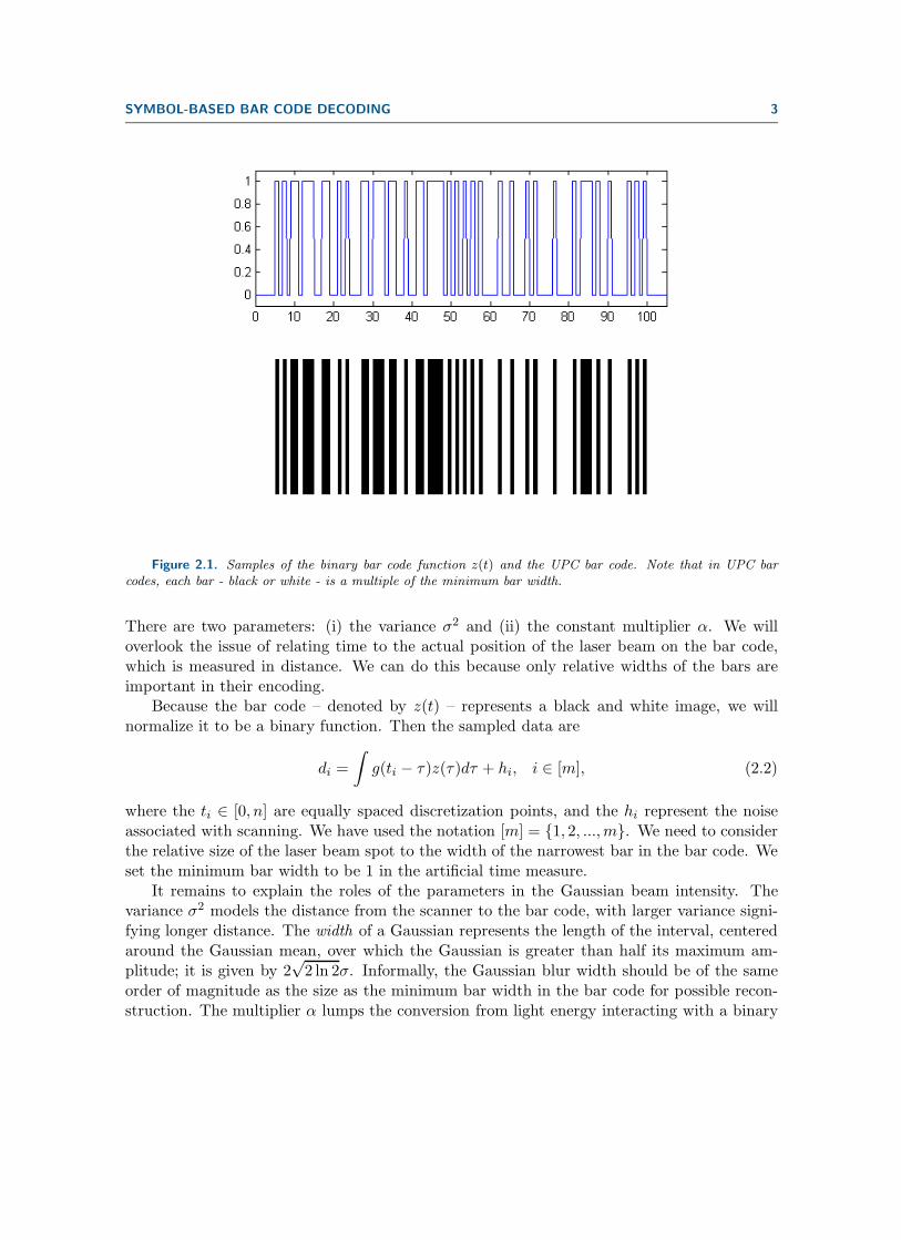
Figure 2.1. Samples of the binary bar code function z(t) and the UPC bar code. Note that in UPC barcodes, each bar - black or white - is a multiple of the minimum bar width.

There are two parameters: (i) the variance σ2 and (ii) the constant multiplier α. We willoverlook the issue of relating time to the actual position of the laser beam on the bar code,which is measured in distance. We can do this because only relative widths of the bars areimportant in their encoding.

Because the bar code – denoted by z(t) – represents a black and white image, we willnormalize it to be a binary function. Then the sampled data are

di =

∫g(ti − τ)z(τ)dτ + hi, i ∈ [m], (2.2)

where the ti ∈ [0, n] are equally spaced discretization points, and the hi represent the noiseassociated with scanning. We have used the notation [m] = {1, 2, ...,m}. We need to considerthe relative size of the laser beam spot to the width of the narrowest bar in the bar code. Weset the minimum bar width to be 1 in the artificial time measure.

It remains to explain the roles of the parameters in the Gaussian beam intensity. Thevariance σ2 models the distance from the scanner to the bar code, with larger variance signi-fying longer distance. The width of a Gaussian represents the length of the interval, centeredaround the Gaussian mean, over which the Gaussian is greater than half its maximum am-plitude; it is given by 2

√2 ln 2σ. Informally, the Gaussian blur width should be of the same

order of magnitude as the size as the minimum bar width in the bar code for possible recon-struction. The multiplier α lumps the conversion from light energy interacting with a binary


bar code image to the measurement. Since the distance to the bar code is unknown and theintensity-to-voltage conversion depends on ambient light and properties of the laser/detector,these parameters are assumed to be unknown.

To develop the model further, consider the characteristic function

χ(t) =

{1 for 0 ≤ t ≤ 1,0 else.

Then the bar code function can be written as

z(t) =

n∑

j=1

cjχ(t− (j − 1)), (2.3)

where the coefficients cj are either 0 or 1 (see, e.g., Figure 2.1). The sequence

c1, c2, · · · , cn,

represents the information stored in the bar code, with a ‘0’ corresponding to a white bar ofunit width and a ‘1’ corresponding to a black bar of unit width. For UPC bar codes, the totalnumber of unit widths, n, is fixed to be 95 for a 12-digit code (further explanations in thesubsequent).

Remark 2.1.One can think of the sequence {c1, c2, · · · , cn} as an instruction for printing abar code. Every ci is a command to lay out a white bar if ci = 0, or a black bar if otherwise.

Substituting the bar code representation (2.3) back in (2.2), the sampled data can be repre-sented as follows:

di =

∫g(ti − t)

n∑

j=1

cjχ(t− (j − 1))

dt+ hi

=

n∑

j=1

[∫ j

(j−1)g(ti − t)dt

]cj + hi.

In terms of the matrix G = G(σ) with entries

Gkj =1√2πσ

∫ j

(j−1)e−

(tk−t)2

2σ2 dt, k ∈ [m], j ∈ [n], (2.4)

the bar code determination problem reads

d = αG(σ)c + h. (2.5)

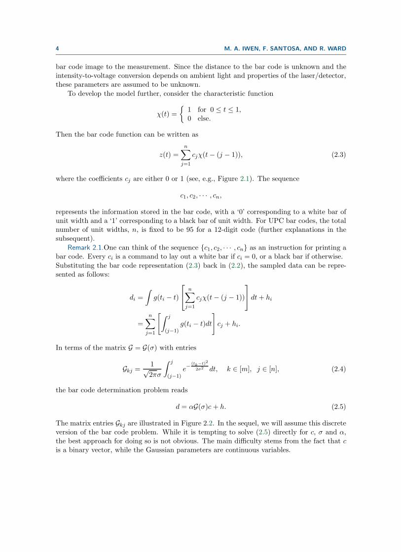
The matrix entries Gkj are illustrated in Figure 2.2. In the sequel, we will assume this discreteversion of the bar code problem. While it is tempting to solve (2.5) directly for c, σ and α,the best approach for doing so is not obvious. The main difficulty stems from the fact that cis a binary vector, while the Gaussian parameters are continuous variables.


tk

0 1 2 3 4 5 6 7 8 9 10t

Figure 2.2. The matrix element Gkj is calculated by placing a scaled Gaussian over the bar code grid andintegrating over each of the bar code intervals.

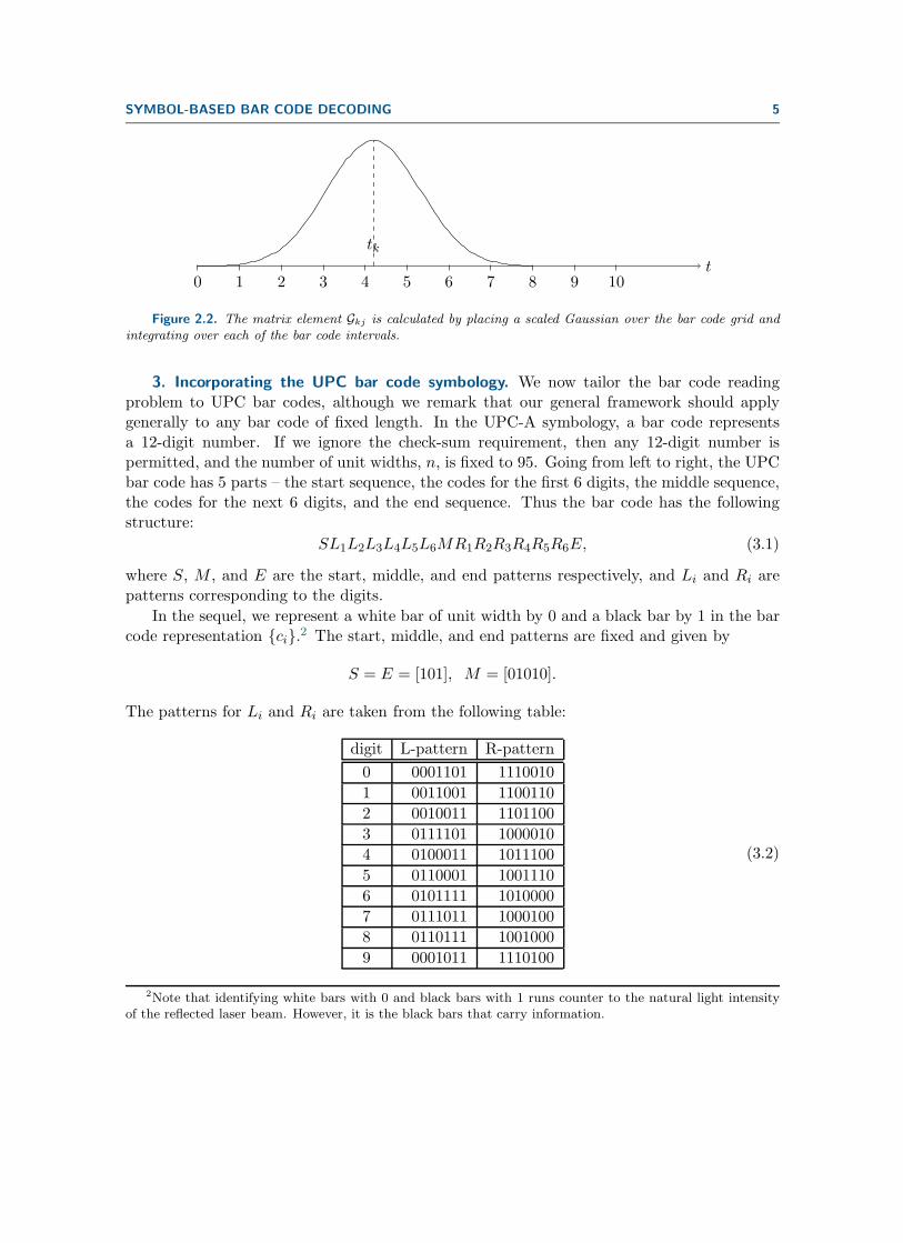
3. Incorporating the UPC bar code symbology. We now tailor the bar code readingproblem to UPC bar codes, although we remark that our general framework should applygenerally to any bar code of fixed length. In the UPC-A symbology, a bar code representsa 12-digit number. If we ignore the check-sum requirement, then any 12-digit number ispermitted, and the number of unit widths, n, is fixed to 95. Going from left to right, the UPCbar code has 5 parts – the start sequence, the codes for the first 6 digits, the middle sequence,the codes for the next 6 digits, and the end sequence. Thus the bar code has the followingstructure:

SL1L2L3L4L5L6MR1R2R3R4R5R6E, (3.1)

where S, M , and E are the start, middle, and end patterns respectively, and Li and Ri arepatterns corresponding to the digits.

In the sequel, we represent a white bar of unit width by 0 and a black bar by 1 in the barcode representation {ci}.2 The start, middle, and end patterns are fixed and given by

S = E = [101], M = [01010].

The patterns for Li and Ri are taken from the following table:

digit L-pattern R-pattern

0 0001101 1110010

1 0011001 1100110

2 0010011 1101100

3 0111101 1000010

4 0100011 1011100

5 0110001 1001110

6 0101111 1010000

7 0111011 1000100

8 0110111 1001000

9 0001011 1110100

(3.2)

2Note that identifying white bars with 0 and black bars with 1 runs counter to the natural light intensityof the reflected laser beam. However, it is the black bars that carry information.


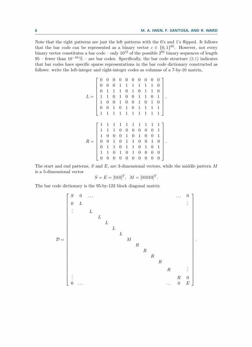
Note that the right patterns are just the left patterns with the 0’s and 1’s flipped. It followsthat the bar code can be represented as a binary vector c ∈ {0, 1}95. However, not everybinary vector constitutes a bar code – only 1012 of the possible 295 binary sequences of length95 – fewer than 10−16% – are bar codes. Specifically, the bar code structure (3.1) indicatesthat bar codes have specific sparse representations in the bar code dictionary constructed asfollows: write the left-integer and right-integer codes as columns of a 7-by-10 matrix,

L =

0 0 0 0 0 0 0 0 0 00 0 0 1 1 1 1 1 1 00 1 1 1 0 1 0 1 1 01 1 0 1 0 0 1 1 0 11 0 0 1 0 0 1 0 1 00 0 1 0 1 0 1 1 1 11 1 1 1 1 1 1 1 1 1

,

R =

1 1 1 1 1 1 1 1 1 11 1 1 0 0 0 0 0 0 11 0 0 0 1 0 1 0 0 10 0 1 0 1 1 0 0 1 00 1 1 0 1 1 0 1 0 11 1 0 1 0 1 0 0 0 00 0 0 0 0 0 0 0 0 0

.

The start and end patterns, S and E, are 3-dimensional vectors, while the middle pattern Mis a 5-dimensional vector

S = E = [010]T , M = [01010]T .

The bar code dictionary is the 95-by-123 block diagonal matrix

D =

S 0 . . . . . . 0

0 L...

... LL

LL

LM

RR

RR

R...

... R 00 . . . . . . 0 E

.


The bar code (3.1), expanded in the bar code dictionary, has the form

c = Dx, x ∈ {0, 1}123 , (3.3)

where

1. The 1st, 62nd and the 123rd entries of x, corresponding to the S, M , and E patterns,are 1.

2. Among the 2nd through 11th entries of x, exactly one entry – the entry correspondingto the first digit in c = Dx – is nonzero. The same is true for 12th through 22nd entries,etc, until the 61st entry. This pattern starts again from the 63rd entry through the122th entry. In all, x has exactly 15 nonzero entries.

That is, x must take the form

xT = [1, vT1 , · · · , vT6 , 1, vT7 , · · · , vT12, 1], (3.4)

where vj , for j = 1, · · · , 12, are vectors in {0, 1}10 having only one nonzero element. In thisnew representation, the bar code reconstruction problem (2.5) reads

d = αG(σ)Dx+ h, (3.5)

where d ∈ Rm is the measurement vector, the matrices G(σ) ∈ R

m×95 and D ∈ {0, 1}95×123

are as defined in (2.4) and (3.3) respectively, and h ∈ Rm is additive noise. Note that D has

fewer rows than columns, while G will generally have more rows than columns; we will refer tothe ratio of rows to columns as the oversampling ratio and denote it by r = m/n. Given thedata d ∈ R

m, our objective is to return a valid bar code x ∈ {0, 1}123 as reliably and quicklyas possible.

4. Properties of the forward map. Incorporating the bar code dictionary into the inverseproblem (3.5), we see that the map between the bar code and observed data is representedby the matrix P = αG(σ)D ∈ R

m×123. We will refer to P, which is a function of the modelparameters α and σ, as the forward map.

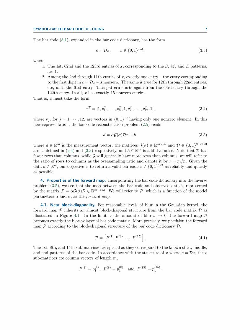
4.1. Near block-diagonality. For reasonable levels of blur in the Gaussian kernel, theforward map P inherits an almost block-diagonal structure from the bar code matrix D asillustrated in Figure 4.1. In the limit as the amount of blur σ → 0, the forward map Pbecomes exactly the block-diagonal bar code matrix. More precisely, we partition the forwardmap P according to the block-diagonal structure of the bar code dictionary D,

P =[P (1) P (2) . . . P (15)

]. (4.1)

The 1st, 8th, and 15th sub-matrices are special as they correspond to the known start, middle,and end patterns of the bar code. In accordance with the structure of x where c = Dx, thesesub-matrices are column vectors of length m,

P (1) = p(1)1 , P (8) = p

(8)1 , and P (15) = p

(15)1 .


The remaining sub-matrices are blurred versions of the left-integer and right-integer codes Land R, represented as m-by-10 nonnegative real matrices. We write each of them as

P (j) =[p(j)1 p

(j)2 . . . p

(j)10

], j 6= 1, 8, 15, (4.2)

where each p(j)k , k = 1, 2, ..., 10, is a column vector of length m.

Figure 4.1. A representative bar code forward map P = αG(σ)D corresponding to oversampling parameterr = 10, amplitude α = 1, and Gaussian standard deviation σ = 1.5. The lone column vectors at the start,middle, and end account for the known start, middle, and end patterns in the bar code.

Recall that the over-sampling rate r = m/n indicates the number of time samples perminimal bar code width. Given r, we can partition the rows of P into 15 blocks, each blockwith index set Ij of size |Ij |, so that each sub-matrix is well-localized within a single block.We know that if P (1) and P (15) correspond to samples of the 3-bar sequence “101” or “black-white-black”, so |I1| = |I15| = 3r. The sub-matrix P (8) corresponds to samples from themiddle 5 bar-sequence so |I8| = 5r. Each remaining sub-matrix corresponds to samples froma digit of length 7 bars, therefore |Ij | = 7r for j 6= 1, 8, 15.

We can now give a quantitative measure describing how ‘block-diagonal’ the forward mapis. To this end, let ε be the infimum of all ǫ > 0 satisfying both

∥∥∥∥p(j)k

∣∣∣[m]\Ij

∥∥∥∥1

< ǫ, for all j ∈ [15], k ∈ [10], (4.3)

and∥∥∥∥∥∥∥

15∑

j′=j+1

p(j′)kj′

∣∣∣∣∣∣Ij

∥∥∥∥∥∥∥1

< ǫ, for all j ∈ [15], and all choices of kj+1, . . . , k15 ∈ [10]. (4.4)

The magnitude of ε indicates to what extent the energy of each column of P is localized withinits proper block. If there were no blur, there would be no overlap between blocks and ǫ = 0.


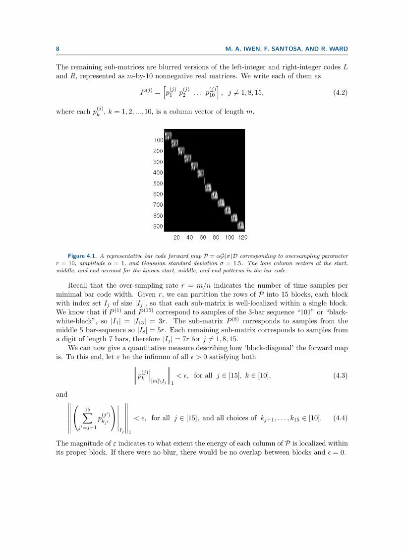
Simulation results such as those in Figure 4.2 suggest that for α = 1, the value of ε in theforward map P can be expressed in terms of the oversampling ratio r and Gaussian standarddeviation σ according to the formula ε = (2/5)σr, at least over the relevant range of blur0 ≤ σ ≤ 1.5. By linearity of the forward map with respect to the amplitude α, this impliesthat more generally ε = (2/5)ασr.

Figure 4.2. For oversampling ratios r = 10 (left) and r = 20 (right) and α = 1, the thick line represents theminimal value of ε satisfying (4.3) and (4.4) in terms of σ. The thin line in each plot represents the function(2/5)σr.

4.2. Column incoherence. We now highlight another property of the forward map P thatallows for robust bar code reconstruction. The left-integer and right-integer codes for the UPCbar code, as enumerated in Table (3.2), are well-separated by design: the ℓ1-distance betweenany two distinct codes is greater than or equal to 2. Consequently, if Dk are the columns ofthe bar code dictionary D, then mink1 6=k2 ‖Dk1−Dk2‖1 = 2. This implies for the forward mapP = αG(σ)D that when there is no blur, i.e. σ = 0,

µ := minj,k1 6=k2

∥∥∥p(j)k1− p

(j)k2

∥∥∥1= min

j,k1 6=k2

∥∥∥∥p(j)k1

∣∣∣Ij− p

(j)k2

∣∣∣Ij

∥∥∥∥1

= 2αr, (4.5)

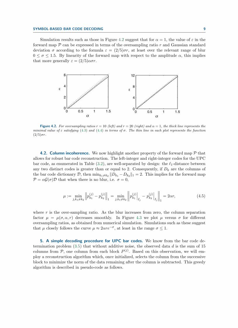
where r is the over-sampling ratio. As the blur increases from zero, the column separationfactor µ = µ(σ, α, r) decreases smoothly. In Figure 4.3 we plot µ versus σ for differentoversampling ratios, as obtained from numerical simulation. Simulations such as these suggestthat µ closely follows the curve µ ≈ 2αre−σ , at least in the range σ ≤ 1.

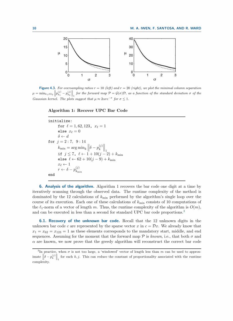
5. A simple decoding procedure for UPC bar codes. We know from the bar code de-termination problem (3.5) that without additive noise, the observed data d is the sum of 15columns from P, one column from each block P (j). Based on this observation, we will em-ploy a reconstruction algorithm which, once initialized, selects the column from the successiveblock to minimize the norm of the data remaining after the column is subtracted. This greedyalgorithm is described in pseudo-code as follows.


Figure 4.3. For oversampling ratios r = 10 (left) and r = 20 (right), we plot the minimal column separation

µ = mink1 6=k2

∥∥∥p(j)k1− p

(j)k2

∥∥∥1for the forward map P = G(σ)D, as a function of the standard deviation σ of the

Gaussian kernel. The plots suggest that µ ≈ 2αre−σ for σ ≤ 1.

Algorithm 1: Recover UPC Bar Code

initialize:

for ℓ = 1, 62, 123, xℓ = 1else xℓ = 0δ ← d

for j = 2 : 7, 9 : 14

kmin = argmink

∥∥∥δ − p(j)k

∥∥∥1

if j ≤ 7, ℓ← 1 + 10(j − 2) + kmin

else ℓ← 62 + 10(j − 9) + kmin

xℓ ← 1r ← δ − p

(j)kmin

end

6. Analysis of the algorithm. Algorithm 1 recovers the bar code one digit at a time byiteratively scanning through the observed data. The runtime complexity of the method isdominated by the 12 calculations of kmin performed by the algorithm’s single loop over thecourse of its execution. Each one of these calculations of kmin consists of 10 computations ofthe ℓ1-norm of a vector of length m. Thus, the runtime complexity of the algorithm is O(m),and can be executed in less than a second for standard UPC bar code proportions.3

6.1. Recovery of the unknown bar code. Recall that the 12 unknown digits in theunknown bar code c are represented by the sparse vector x in c = Dx. We already know thatx1 = x62 = x123 = 1 as these elements corresponds to the mandatory start, middle, and endsequences. Assuming for the moment that the forward map P is known, i.e., that both σ andα are known, we now prove that the greedy algorithm will reconstruct the correct bar code

3In practice, when σ is not too large, a ‘windowed’ vector of length less than m can be used to approx-

imate∥∥∥δ − p

(j)k

∥∥∥1for each k, j. This can reduce the constant of proportionality associated with the runtime

complexity.


from noisy data d = Px + h as long as P is sufficiently block-diagonal and if its columns aresufficiently incoherent. In the next section we will extend the analysis to the case where σand α are unknown.

Theorem 1.Suppose I1, . . . , I15 ⊂ [m] and ε ∈ R satisfy the conditions (4.3)-(4.4). Then,Algorithm 1 will correctly recover a bar code signal x from noisy data d = Px + h providedthat ∥∥∥∥p

(j)k1

∣∣∣Ij− p

(j)k2

∣∣∣Ij

∥∥∥∥1

> 2(∥∥h|Ij

∥∥1+ 2ε

)(6.1)

for all j ∈ [15] and k1, k2 ∈ [10] with k1 6= k2.

Proof:

Suppose that

d = Px+ h =

15∑

j=1

p(j)kj

+ h.

Furthermore, denoting kj = kmin in the for-loop in Algorithm 1, suppose that k2, . . . , kj′−1

have already been correctly recovered. Then the residual data, δ, at this stage of the algorithmwill be

δ = p(j′)kj′

+ δj′ + h,

where δj′ is defined to be

δj′ =

15∑

j=j′+1

p(j)kj

.

We will now show that the j′th execution of the for-loop will correctly recover p(j′)kj′

, thereby

establishing the desired result by induction.

Suppose that the j′th execution of the for-loop incorrectly recovers kerr 6= kj′ . Thishappens if ∥∥∥δ − p

(j′)kerr

∥∥∥1≤∥∥∥δ − p

(j′)kj′

∥∥∥1.

In other words, we have that

∥∥∥δ − p(j′)kerr

∥∥∥1=

∥∥∥∥δ∣∣Ij′− p

(j′)kerr

∣∣∣Ij′

∥∥∥∥1

+

∥∥∥∥∥δ∣∣Icj′− p

(j′)kerr

∣∣∣Icj′

∥∥∥∥∥1

≥∥∥∥∥p

(j′)kj′

∣∣∣Ij′− p

(j′)kerr

∣∣∣Ij′

∥∥∥∥1

−∥∥∥δj′

∣∣Ij′

∥∥∥1−∥∥∥h∣∣Ij′

∥∥∥1

+

∥∥∥∥δj′∣∣Icj′+ h∣∣Icj′

∥∥∥∥1

−∥∥∥∥∥p

(j′)k′j

∣∣∣Icj′

∥∥∥∥∥1

−∥∥∥∥∥p

(j′)kerr

∣∣∣Icj′

∥∥∥∥∥1

≥∥∥∥∥p

(j′)kj′

∣∣∣Ij′− p

(j′)kerr

∣∣∣Ij′

∥∥∥∥1

+

∥∥∥∥δj′∣∣Icj′+ h∣∣Icj′

∥∥∥∥1

−∥∥∥h∣∣Ij′

∥∥∥1− 3ε


from conditions (4.3) and (4.4). To finish, we simply simultaneously add and subtract ‖δj′ |Ij′+h|Ij′‖1 from the last expression to arrive at a contradiction to the supposition that kerr 6= kj′ :

∥∥∥δ − p(j′)kerr

∥∥∥1≥(∥∥∥∥p

(j′)kj′

∣∣∣Ij′− p

(j′)kerr

∣∣∣Ij′

∥∥∥∥1

− 2∥∥∥h∣∣Ij′

∥∥∥1− 4ε

)+∥∥δj′ + h

∥∥1

=

(∥∥∥∥p(j′)kj′

∣∣∣Ij′− p

(j′)kerr

∣∣∣Ij′

∥∥∥∥1

− 2∥∥∥h∣∣Ij′

∥∥∥1− 4ε

)+∥∥∥δ − p

(j′)kj′

∥∥∥1

>∥∥∥δ − p

(j′)kj′

∥∥∥1. (6.2)

�Remark 6.1. Equation (4.3) implies that

minj,k1 6=k2

∥∥∥∥p(j)k1

∣∣∣Ij− p

(j)k2

∣∣∣Ij

∥∥∥∥1

≥ minj,k1 6=k2

∥∥∥p(j)k1− p

(j)k2

∥∥∥1− 2ε = µ− 2ε.4

Thus, the recovery condition (6.1) in Theorem 1 will hold whenever

µ− 2ε > 2(∥∥h|Ij

∥∥1+ 2ε

).

Using the empirical relationships ε = (2/5)αrσ and µ = 2αre−σ , we obtain the followingupper bound on the level of sufficient noise for successful recovery:

maxj∈[12]

∥∥h|Ij∥∥1< αr(e−σ − (6/5)σ). (6.3)

In practice the Gaussian blur width 2√

2 ln(2)σ does not exceed the minimum width of thebar code, which we have normalized to be 1. This translates to a maximal standard deviationof σ ≈ .425, and a noise ceiling in (6.3) of

maxj∈[12]

∥∥h|Ij∥∥1≤ .144αr. (6.4)

This should be compared to the ℓ1-norm of the bar code signal over a block; the average ℓ1norm between the left-integer and right-integer codes is 3.5α.

Remark 6.2. In practice it may be beneficial to apply Algorithm 1 several times, each timechanging the order in which the digits are decoded. For example, if the distribution of thenoise is known in advance, it would be beneficial to to initialize the algorithm in regions ofthe bar code with less noise.

6.2. Stability of the greedy algorithm with respect to parameter estimation.

Insensitivity to unknown α. In the previous section we assumed a known Gaussian con-volution matrix αG(σ). In fact, this is generally not the case. In practice both σ and α mustbe estimated since these parameters depend on the distance from the scanner to the bar code,the reflectivity of the scanned surface, the ambient light, etc. This means that in practice,

4See equation (4.5) for the definition of µ.


Algorithm 1 will be decoding bar codes using only an approximation to αG(σ). Suppose thatthe true standard deviation generating a sampled sequence d is σ, but that Algorithm 1 usesa different value σ̂ for reconstruction. We can regard the error incurred by σ̂ as additionaladditive noise in our sensitivity analysis, setting h′ = h + α

(G(σ) − G(σ̂)

)Dx and rewriting

the inverse problem as

d = αG(σ)Dx + h

= αG(σ̂)Dx+(h+ α

(G(σ)− G(σ̂)

)Dx)

= αG(σ̂)Dx+ h′. (6.5)

We now describe a procedure for estimating α. Note that the middle portion of the observeddata of length 5r, dmid = d|I8 , represents a blurry image of the known middle pattern M =[01010]. Let P = G(σ̂)D be the forward map generated by the estimate σ̂ when α = 1, andconsider the sub-matrix

pmid = P (8)∣∣∣I8

which is also a vector of length 5r. If σ̂ = σ or σ̂ ≈ σ,5 we expect a good estimate for α to bethe least squares solution

α̂ = argmina‖apmid − dmid‖2 = pTmiddmid/‖ pmid‖22. (6.6)

Dividing both sides of the equation (6.5) by α̂, the inverse problem becomes

d

α̂=

α

α̂G(σ̂)Dx+

1

α̂h′. (6.7)

Suppose that 1 − γ ≤ α/α̂ ≤ 1 + γ for some 0 < γ < 1. Then fixing the data to bed̂ = d/α̂ and fixing forward map to be P = G(σ̂)D, the recovery conditions (4.3), (4.4), and(6.1) become respectively

1.

∥∥∥∥p(j)k

∣∣∣[m]\Ij

∥∥∥∥1

< ε1+γ for all j ∈ [15] and k ∈ [10].

2.

∥∥∥∥(∑15

j′=j+1 p(j′)kj′

)∣∣∣Ij

∥∥∥∥1

< ε1+γ for all j ∈ [14] and valid kj′ ∈ [10].

3.

∥∥∥∥p(j)k1

∣∣∣Ij− p

(j)k2

∣∣∣Ij

∥∥∥∥1

> 2(

1α

∥∥∥h|Ij∥∥∥1+∥∥∥(G(σ) − G(σ̂)

)Dx∣∣Ij

∥∥∥1+ 2ε

1−γ

)

Consequently, if σ ≈ σ̂ and 1 / α ≈ α̂, the conditions for correct bar code reconstruction donot change much.

Insensitivity to unknown σ. We have seen that one way to estimate the scaling α is toguess a value for σ and perform a least-squares fit of the observed data. In doing so, we foundthat the sensitivity of the recovery process with respect to σ is proportional to the quantity

∥∥∥(G(σ) − G(σ̂))Dx|Ij∥∥∥1

(6.8)

5Here we have assumed that the noise level is low. In noisier settings it should be possible to develop moreeffective methods for estimating α by incorporating the characteristics of the scanning noise.


in the third condition immediately above. Note that all the entries of the matrix G(σ)−G(σ̂)will be small whenever σ̂ ≈ σ. Thus, Algorithm 1 should be able to tolerate small parameterestimation errors as long as the “almost” block diagonal matrix formed using σ̂ exhibits asizable difference between any two of its digit columns which might (approximately) appearin any position of a given UPC bar code.

To get a sense of the size of the term (6.8), let us further investigate the expressionsinvolved. Recall that using the dictionary matrix D, a bar code sequence of 0’s and 1’s isgiven by c = Dx. When put together with the bar code function representation (2.3), we seethat

[G(σ)Dx]i =∫

gσ(ti − t)z(t)dt,

where

gσ(t) =1√2πσ

e−( t2

2σ2 ).

Therefore, we have

[G(σ)Dx]i =n∑

j=1

cj

∫ j

j−1gσ(ti − t)dt. (6.9)

Now, using the definition for the cumulative distribution function for normal distributions

Φ(x) =1√2π

∫ x

−∞e−t2/2dt,

we see that ∫ j

j−1gσ(ti − t)dt = Φ

(ti − j + 1

σ

)− Φ

(ti − j

σ

).

and we can now rewrite (6.9) as

[G(σ)Dx]i =n∑

j=1

cj

[Φ

(ti − j + 1

σ

)− Φ

(ti − j

σ

)].

We now isolate the term we wish to analyze:

[(G(σ) − G(σ̂))Dx]i

=n∑

j=1

cj

[Φ

(ti − j + 1

σ

)− Φ

(ti − j + 1

σ̂

)− Φ

(ti − j

σ

)+Φ

(ti − j

σ̂

)].

We are interested in the error

|[(G(σ)− G(σ̂))Dx]i|

≤n∑

j=1

cj

∣∣∣∣Φ(ti − j + 1

σ

)− Φ

(ti − j + 1

σ̂

)− Φ

(ti − j

σ

)+Φ

(ti − j

σ̂

)∣∣∣∣

≤n∑

j=1

∣∣∣∣Φ(ti − j + 1

σ

)− Φ

(ti − j + 1

σ̂

)∣∣∣∣+∣∣∣∣Φ(ti − j

σ

)− Φ

(ti − j

σ̂

)∣∣∣∣ ,

≤ 2n∑

j=0

∣∣∣∣Φ(ti − j

σ

)− Φ

(ti − j

σ̂

)∣∣∣∣ .


Suppose that ξ = (ξk) is the vector of values |ti − j| for fixed i, running j, sorted in orderof increasing magnitude. Note that ξ1 and ξ2 are less than or equal to 1, and ξ3 ≤ ξ1 + 1,ξ4 ≤ ξ2 + 1, and so on. We can center the previous bound around ξ1 and ξ2, giving

|[(G(σ) − G(σ̂))Dx]i| ≤n∑

j=0

∣∣∣∣Φ(ξ1 + j

σ

)−Φ

(ξ1 + j

σ̂

)∣∣∣∣+∣∣∣∣Φ(ξ2 + j

σ

)− Φ

(ξ2 + j

σ̂

)∣∣∣∣ .(6.10)

Next we simply majorize the expression

f(x) = Φ(xσ

)− Φ

(xσ̂

).

To do so, we take the derivative and find the critical points, which turn out to be

x∗ = ±√2σσ̂

√log σ − log σ̂

σ2 − σ̂2.

Therefore, each term in the summand (6.10) can be bounded by

∣∣∣∣Φ(ξ + j

σ

)− Φ

(ξ + j

σ̂

)∣∣∣∣ ≤∣∣∣∣∣Φ(√2σ̂


σ2 − σ̂2

)− Φ

(√2σ


σ2 − σ̂2

)∣∣∣∣∣:= △1(σ, σ̂). (6.11)

On the other hand, the terms in the sum decrease exponentially as j increases. To seethis, recall the simple bound

1− Φ(x) =1√2π

∫ ∞

xe−t2/2dt ≤ 1√

2π

∫ ∞

x

t

xe−t2/2dt =

e−x2/2

x√2π

.

Writing σmax = max{(σ, σ̂)}, and noting that Φ(x) is a positive, increasing function, we havefor ξ ∈ [0, 1)

∣∣∣∣Φ(ξ + j

σ

)− Φ

(ξ + j

σ̂

)∣∣∣∣ ≤ 1− Φ

(ξ + j

σmax

)

≤ σmax

(ξ + j)√2π

e−(ξ+j)2/(2σ2max)

≤ σmax

(ξ + j)√2π

e−(ξ+j)/(2σ2max) if j ≥ 1

=σmax

(ξ + j)√2π

(e−(2σ2

max)−1)ξ+j

≤ σmax

j√2π

(e−(2σ2

max)−1)j

:= ∆2(σmax, j). (6.12)

Combining the bounds (6.11) and (6.12),∣∣∣∣Φ(ξ + j

σ

)−Φ

(ξ + j

σ̂

)∣∣∣∣ ≤ min((△1(σ, σ̂),△2(σmax, j)

).


Suppose that j1 is the smallest integer in absolute value such that △2(σmax, j1) ≤ △1(σ, σ̂).Then from this term on, the summands in (6.10) can be bounded by a geometric series:

n∑

j≥j1

∣∣∣∣Φ(ξ + j

σ

)− Φ

(ξ + j

σ̂

)∣∣∣∣ ≤2σmax

j1√2π

∑

j≥j1

aj, a = e−(2σ2max)

−1

≤ 2σmax

j1√2π· aj1(1− a)−1.

We then arrive at the bound

|[(G(σ)− G(σ̂))Dx]i| ≤ 2 · j1△1(σ, σ̂) +4σmax · aj1(1− a)−1

j1√2π

=: B(σ, σ̂). (6.13)

The term (6.8) can then be bounded according to

∥∥∥(G(σ)− G(σ̂))Dx|Ij∥∥∥1≤ |Ij|B(σ, σ̂) ≤ 7rB(σ, σ̂), (6.14)

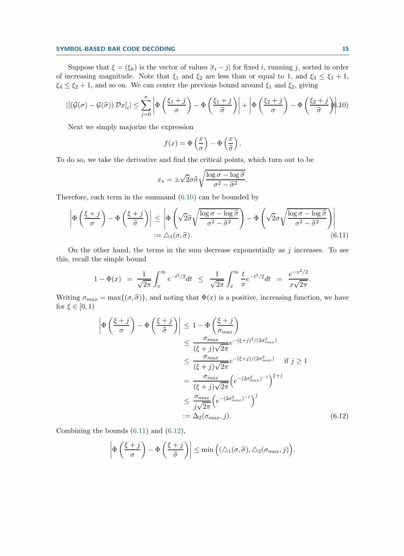
where r = m/n is the over-sampling rate.Recall that in practice the width 2

√2 ln(2)σ of the Gaussian kernel is on the order of the

minimum bar width in the bar code, which we normalized to 1. When the blur exactly equalsthe minimum bar width, we arrive at σ ≈ .425. Below, we compute the error bound B(σ, σ̂)for σ = .425 and several values of σ̂.

σ̂ 0.2 0.4 .5 0.6 .8

B(.425, σ̂) .3453 .0651 .1608 .3071 .589

While the bound (6.14) is very rough, note that the tabulated error bounds incurred byinaccurate σ are at least roughly the same order of magnitude as the empirical noise leveltolerance for the greedy algorithm, as discussed in Remark 6.1.

7. Numerical Evaluation. In this section we illustrate with numerical examples the ro-bustness of the greedy algorithm to signal noise and imprecision in the α and σ parameterestimates. We assume that neither α nor σ is known a priori, but that we have an estimateσ̂ for σ. We then compute an estimate α̂ from σ̂ by solving the least-squares problem (6.6).

The phase diagrams in Figure 7.1 demonstrate the insensitivity of the greedy algorithm torelatively large amounts of noise. These diagrams were constructed by executing Algorithm1 on many trial input signals of the form d = αG(σ)Dx + h, where h is mean zero Gaussiannoise. More specifically, each trial signal, d, was formed as follows: a 12 digit number was firstgenerated uniformly at random, and its associated blurred bar code, αG(σ)Dx, was formedusing the oversampling ratio r = m/n = 10. Second, a noise vector n with independentand identically distributed entries nj ∼ N (0, 1) was generated and then rescaled to form

the additive noise vector h = ν‖αG(σ)Dx‖2 (n/‖n‖2). Hence, the parameter ν = ‖h‖2‖αG(σ)Dx‖2

represents the noise-to-signal ratio of each trial input signal d.We note that in laser-based scanners, there are two major sources of noise: electronic noise

[9], which is often modeled as 1/f noise [5], and speckle noise [10], caused by the roughness


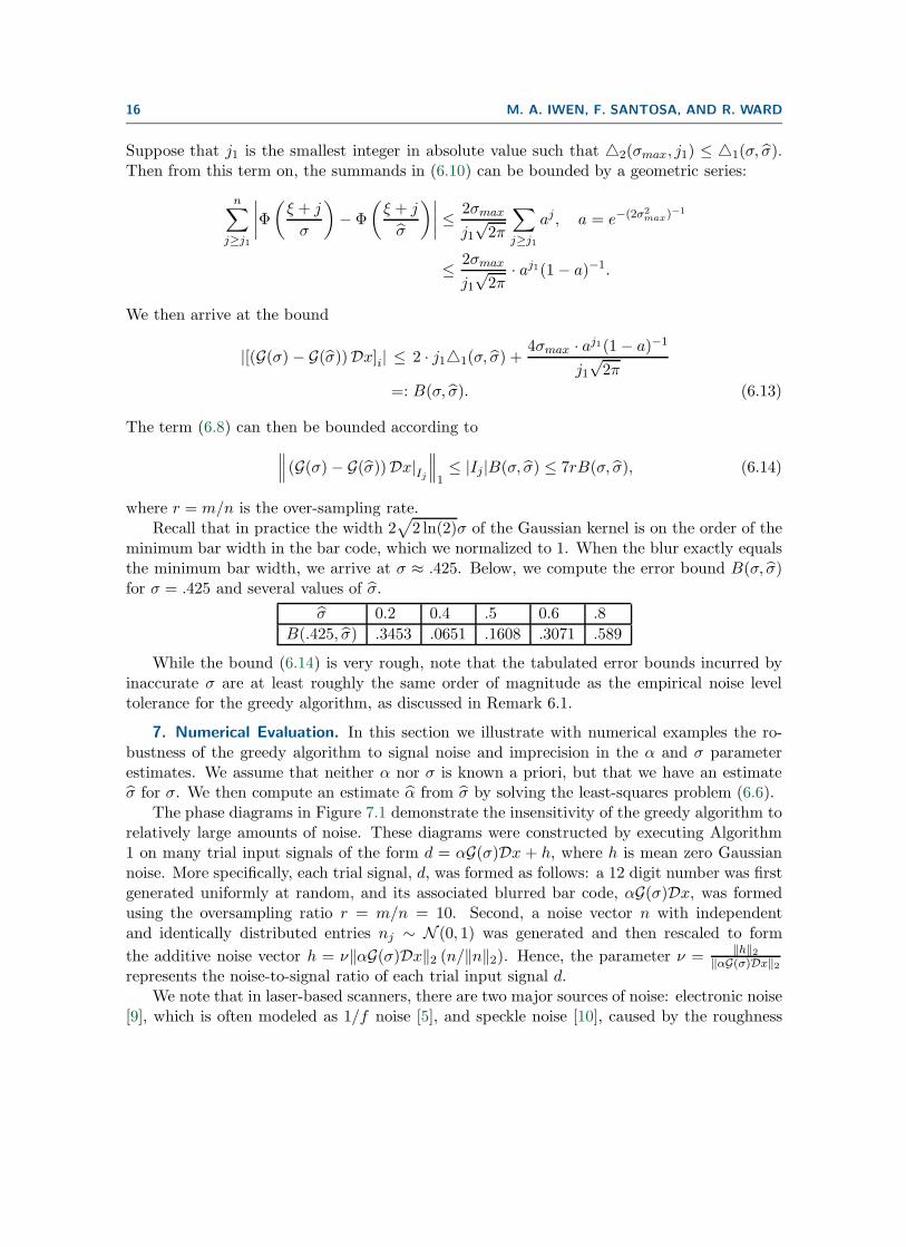
(a) True parameter values: σ = .45, α = 1. (b) True parameter values: σ = .75, α = 1

Figure 7.1. Recovery Probabilities when α = 1 for two true σ settings. The shade in each phase diagramcorresponds to the probability that the greedy algorithm will correctly recover a randomly selected bar code, asa function of the relative noise-to-signal level, ν = ‖h‖2

‖αG(σ)Dx‖2, and the σ estimate, σ̂. Black represents correct

bar code recovery with probability 1, while pure white represents recovery with probability 0. Each data point’sshade (i.e., probability estimate) is based on 100 random trials.

of the paper. However, the Gaussian noise used in our numerical experiments is sufficient forthe purpose of this work.

To create the phase diagrams in Figure 7.1, the greedy recovery algorithm was run on 100independently generated trial input signals for each of at least 100 equally spaced (σ̂, ν) gridpoints (a 10 × 10 mesh was used for Figure 7.1(a), and a 20 × 20 mesh for Figure 7.1(b)).The number of times the greedy algorithm successfully recovered the original UPC bar codedetermined the color of each region in the (σ̂, ν)-plane. The black regions in the phase diagramsindicate regions of parameter values where all 100 of the 100 randomly generated bar codeswere correctly reconstructed. The pure white parameter regions indicate where the greedyrecovery algorithm failed to correctly reconstruct any of the 100 randomly generated bar codes.

Looking at Figure 7.1 we can see that the greedy algorithm appears to be highly robust toadditive noise. For example, when the σ estimate is accurate (i.e., when σ̂ ≈ σ) we can see thatthe algorithm can tolerate additive noise with Euclidean norm as high as 0.25‖αG(σ)Dx‖2 .Furthermore, as σ̂ becomes less accurate the greedy algorithm’s accuracy appears to degradesmoothly.

The phase diagrams in Figures 7.2 and 7.3 more clearly illustrate how the reconstructioncapabilities of the greedy algorithm depend on σ, α, the estimate of σ, and on the noiselevel. We again consider Gaussian additive noise on the signal, i.e. we consider the inverseproblem d = αG(σ)Dx + h, with independent and identically distributed hj ∼ N (0, ξ2), forseveral noise standard deviation levels ξ ∈ [0, .63]. Note that E

( ∥∥h|Ij∥∥1

)= 7rξ

√2/π.6 Thus,

the numerical results are consistent with the bounds in Remark 6.1. Each phase diagramcorresponds to different underlying parameter values (σ, α), but in all diagrams we fix theoversampling ratio at r = m/n = 10. As before, the black regions in the phase diagramsindicate parameter values (σ̂, ξ) for which 100 out of 100 randomly generated bar codes werereconstructed, and white regions indicate parameter values for which 0 out of 100 randomlygenerated bar codes were reconstructed.

Comparing Figures 7.2(a) and 7.3(a) with Figures 7.2(b) and 7.3(b), respectively, we can

6This follows from the fact that the first raw absolute moment of each hj , E(|hj |), is ξ√

2/π.


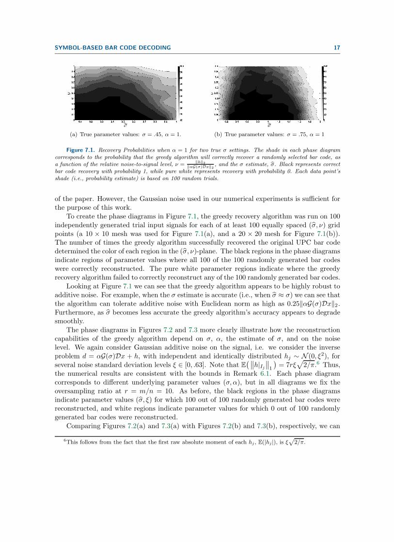
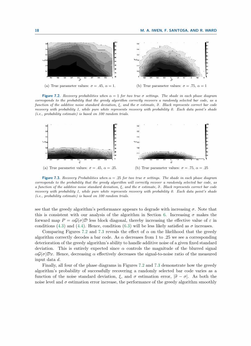
(a) True parameter values: σ = .45, α = 1. (b) True parameter values: σ = .75, α = 1

Figure 7.2. Recovery probabilities when α = 1 for two true σ settings. The shade in each phase diagramcorresponds to the probability that the greedy algorithm correctly recovers a randomly selected bar code, as afunction of the additive noise standard deviation, ξ, and the σ estimate, σ̂. Black represents correct bar coderecovery with probability 1, while pure white represents recovery with probability 0. Each data point’s shade(i.e., probability estimate) is based on 100 random trials.

(a) True parameter values: σ = .45, α = .25. (b) True parameter values: σ = .75, α = .25

Figure 7.3. Recovery Probabilities when α = .25 for two true σ settings. The shade in each phase diagramcorresponds to the probability that the greedy algorithm will correctly recover a randomly selected bar code, asa function of the additive noise standard deviation, ξ, and the σ estimate, σ̂. Black represents correct bar coderecovery with probability 1, while pure white represents recovery with probability 0. Each data point’s shade(i.e., probability estimate) is based on 100 random trials.

see that the greedy algorithm’s performance appears to degrade with increasing σ. Note thatthis is consistent with our analysis of the algorithm in Section 6. Increasing σ makes theforward map P = αG(σ)D less block diagonal, thereby increasing the effective value of ε inconditions (4.3) and (4.4). Hence, condition (6.3) will be less likely satisfied as σ increases.

Comparing Figures 7.2 and 7.3 reveals the effect of α on the likelihood that the greedyalgorithm correctly decodes a bar code. As α decreases from 1 to .25 we see a correspondingdeterioration of the greedy algorithm’s ability to handle additive noise of a given fixed standarddeviation. This is entirely expected since α controls the magnitude of the blurred signalαG(σ)Dx. Hence, decreasing α effectively decreases the signal-to-noise ratio of the measuredinput data d.

Finally, all four of the phase diagrams in Figures 7.2 and 7.3 demonstrate how the greedyalgorithm’s probability of successfully recovering a randomly selected bar code varies as afunction of the noise standard deviation, ξ, and σ estimation error, |σ̂ − σ|. As both thenoise level and σ estimation error increase, the performance of the greedy algorithm smoothly


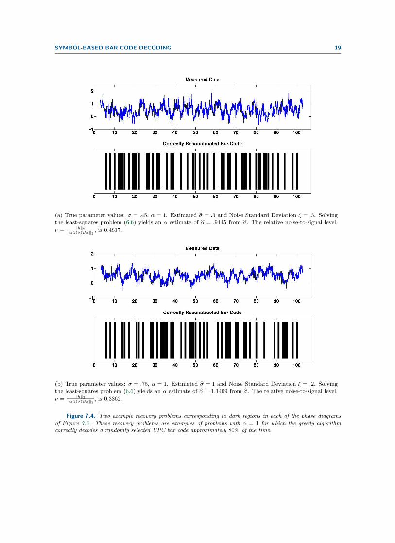
(a) True parameter values: σ = .45, α = 1. Estimated σ̂ = .3 and Noise Standard Deviation ξ = .3. Solvingthe least-squares problem (6.6) yields an α estimate of α̂ = .9445 from σ̂. The relative noise-to-signal level,

ν = ‖h‖2‖αG(σ)Dx‖2

, is 0.4817.

(b) True parameter values: σ = .75, α = 1. Estimated σ̂ = 1 and Noise Standard Deviation ξ = .2. Solvingthe least-squares problem (6.6) yields an α estimate of α̂ = 1.1409 from σ̂. The relative noise-to-signal level,

ν = ‖h‖2‖αG(σ)Dx‖2

, is 0.3362.

Figure 7.4. Two example recovery problems corresponding to dark regions in each of the phase diagramsof Figure 7.2. These recovery problems are examples of problems with α = 1 for which the greedy algorithmcorrectly decodes a randomly selected UPC bar code approximately 80% of the time.


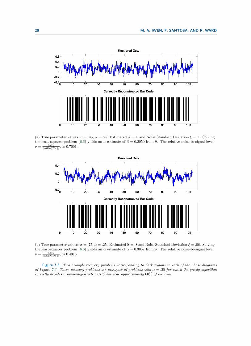
(a) True parameter values: σ = .45, α = .25. Estimated σ̂ = .5 and Noise Standard Deviation ξ = .1. Solvingthe least-squares problem (6.6) yields an α estimate of α̂ = 0.2050 from σ̂. The relative noise-to-signal level,

ν = ‖h‖2‖αG(σ)Dx‖2

, is 0.7001.

(b) True parameter values: σ = .75, α = .25. Estimated σ̂ = .8 and Noise Standard Deviation ξ = .06. Solvingthe least-squares problem (6.6) yields an α estimate of α̂ = 0.3057 from σ̂. The relative noise-to-signal level,

ν = ‖h‖2‖αG(σ)Dx‖2

, is 0.4316.

Figure 7.5. Two example recovery problems corresponding to dark regions in each of the phase diagramsof Figure 7.3. These recovery problems are examples of problems with α = .25 for which the greedy algorithmcorrectly decodes a randomly-selected UPC bar code approximately 60% of the time.


degrades. Most importantly, we can see that the greedy algorithm is relatively robust toinaccurate σ estimates at low noise levels. When ξ ≈ 0 the greedy algorithm appears to sufferonly a moderate decline in reconstruction rate even when |σ̂ − σ| ≈ σ.

Figure 7.4 gives examples of two bar codes which the greedy algorithm correctly recoverswhen α = 1, one for each value of σ presented in Figure 7.2. In each of these examples thenoise standard deviation, ξ, and estimated σ value, σ̂, were chosen so that they correspondto dark regions of the example’s associated phase diagram in Figure 7.2. Hence, these twoexamples represent noisy recovery problems for which the greedy algorithm correctly decodesthe underlying UPC bar code with relatively high probability.7 Similarly, Figure 7.5 gives twoexamples of two bar codes which the greedy algorithm correctly recovered when α = 0.25.Each of these examples has parameters that correspond to a dark region in one of the Figure 7.3phase diagrams.

8. Discussion. In this work, we present a greedy algorithm for the recovery of bar codesfrom signals measured with a laser-based scanner. So far we have shown that the method isrobust to both additive Gaussian noise and parameter estimation errors. There are severalissues that we have not addressed that deserve further investigation.

First, we assumed that the start of the signal is well determined. By the start of thesignal, we mean the time on the recorded signal that corresponds to when the laser firststrikes a black bar. This assumption may be overly optimistic if there is a lot of noise in thesignal. Preliminary numerical experiments suggest that the algorithm is not overly sensitiveto uncertainties in the start time, and we are currently working on the development of a fastpreprocessing algorithm for locating the start position from the samples.

Second, while our investigation shows that the algorithm is not sensitive to the parameterσ in the model, we did not address the best means for obtaining reasonable approximationsto σ. In applications where the scanner distance from the bar code may vary (e.g., withhandheld scanners) other techniques for determining σ̂ will be required. Given the robustnessof the algorithm to parameter estimation errors it may be sufficient to simply fix σ̂ to be theexpected optimal σ parameter value in such situations. In situations where more accuracy isrequired, the hardware might be called on to provide an estimate of the scanner distance fromthe bar code it is scanning, which could then be used to help produce a reasonable σ̂ value.In any case, we leave more careful consideration of methods for estimating σ to future work.

The final assumption we made was that the intensity distribution is well modeled by aGaussian. This may not be sufficiently accurate for some distances between the scanner andthe bar code. Since intensity profile as a function of distance can be measured, one canconceivably refine the Gaussian model to capture the true behavior of the intensities.

REFERENCES

[1] M. Bern and D. Goldberg, Scanner-model-based document image improvement, Proceedings. 2000International Conference on Image Processing, IEEE, 2000, 582–585.

7The ξ and σ̂ values were chosen to correspond to dark regions in a Figure 7.2 phase diagram, not necessarilyto purely black regions.


[2] R. Choksi and Y. van Gennip, Deblurring of one-dimensional bar codes via total variation energyminimisation, SIAM J. Imaging Sciences, 3-4 (2010), pp. 735–764.

[3] R. Choksi, Y. van Gennip, and A. Oberman, Anisotropic total variation regularized L1-approximationand denoising/deblurring of 2D bar codes, Inverse Problems and Imaging, 5 (2011), 591–617.

[4] L. Dumas, M. El Rhabi and G. Rochefort, An evolutionary approach for blind deconvolution ofbarcode images with nonuniform illumination, IEEE Congress on Evolutionary Computation, 2011,2423–2428.

[5] P. Dutta and P. M. Horn, Low-frequency fluctuations in solids: 1/f noise, Rev. Mod. Phys., 53-3(1981), 497–516.

[6] S. Esedoglu, Blind deconvolution of bar code signals, Inverse Problems, 20 (2004), 121–135.[7] S. Esedoglu and F. Santosa, Error estimates for a bar code reconstruction method, to appear in

Discrete and Continuous Dynamical Systems B.[8] J. Kim and H. Lee, Joint nonuniform illumination estimation and deblurring for bar code signals, Optic

Express, 15-22 (2007), 14817–14837.[9] S. Kogan, Electronic Noise and Fluctuations in Solids, Cambridge University Press, 1996.

[10] E. Marom, S. Kresic-Juric and L. Bergstein, Analysis of speckle noise in bar-code scanning systems,J. Opt. Soc. Am., 18 (2001), 888–901.

[11] L. Modica and S. Mortola, Un esempio di Γ–convergenza, Boll. Un. Mat. Ital., 5-14 (1977), 285–299.[12] D. Salomon, Data Compression: The Complete Reference, Springer-Verlag New York Inc, 2004.

A SYMBOL-BASED ALGORITHM FOR DECODING BAR CODES · The multiplier α lumps the conversion from...

Documents

Transcript of A SYMBOL-BASED ALGORITHM FOR DECODING BAR CODES · The multiplier α lumps the conversion from...