1

`

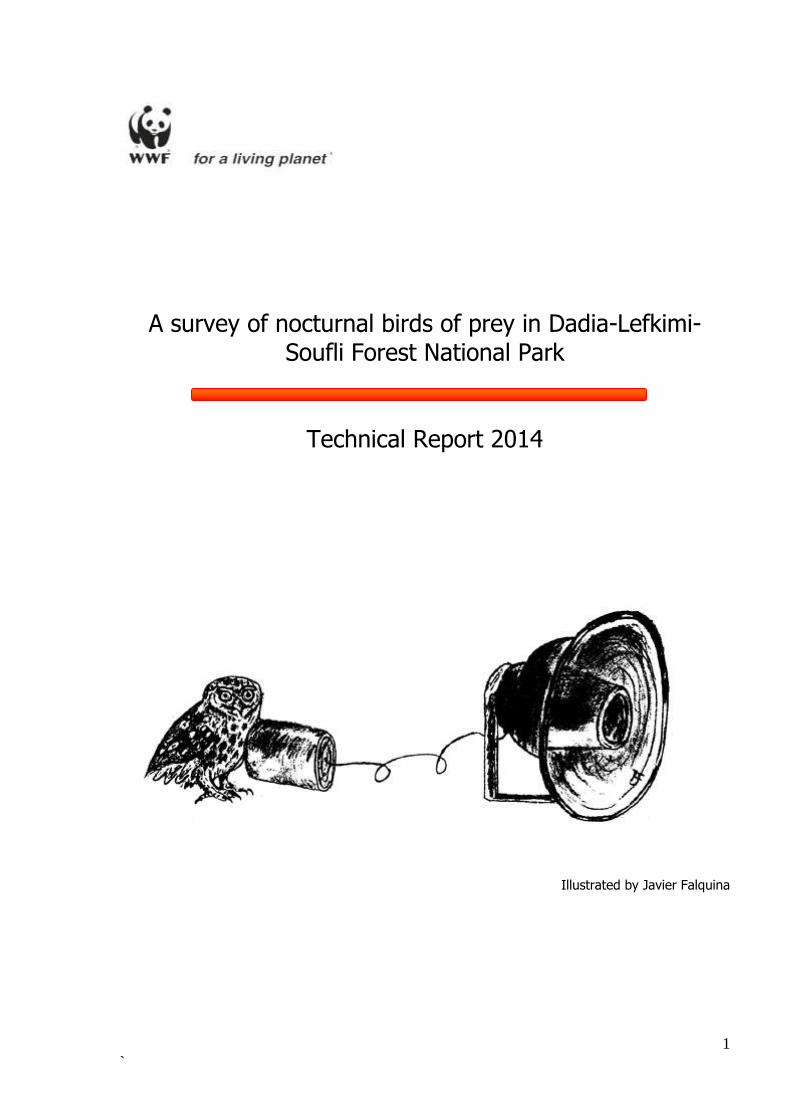
A survey of nocturnal birds of prey in Dadia-Lefkimi-Soufli Forest National Park

Technical Report 2014

Illustrated by Javier Falquina

2

`

WWF Greece 21 Lempesi str. GR- 117 43 ΑTHENS Τel: 0030 2103314893 WWF Greece Evros Project, Dadia, GR- 684 00 Soufli Τel: 0030 2554032210, e-mail : ecodadia@otenet.gr

The present report was carried out with the generous support of the A.G. Leventis Foundation.

This report should be referenced as follows: Kret, E., Pomarède, L., Ruiz, C., Skartsi, Th. & Poirazidis, K. 2014. A survey of nocturnal birds of prey in Dadia-Lefkimi-Soufli Forest National Park. Technical Report 2014, pp. 45. WWF Greece, Athens.

3

`

CONTENTS

0. SUMMARY 1. INTRODUCTION 2. METHODS 2.1. STUDY AREA AND DURATION 2.2. SURVEY POINTS 2.3. FIELD SURVEY 2.4. HABITAT SUITABILTY MODELING

3. RESULTS 3.1. SPECIES DISTRIBUTION 3.2. HABITAT SUITABILTY MODELING 3.2.1. EVALUATION OF THE MODELS 3.2.2. MODEL PER SPECIES

4. DISCUSSION AND RECOMMENDATIONS 4.1. HABITAT PREFERENCES 4.2. THE PLAYBACK METHOD EFFICIENCY 4.3. RECOMMENDATIONS ON SURVEY METHODS FOR FUTURE APPLICATION

5. REFERENCES 6. APPENDICES

4

`

0. SUMMARY The populations of birds of prey are one of the most important ecological features of Dadia-Lefkimi–Soufli Forest National Park. Birds of prey are considered as important ecological indicators revealing the quality of the ecosystem, indicating environmental pollution as well as habitat degradation and destruction. This survey was focused strictly on nocturnal owls and was carried out between January 2012 and March 2013. We searched for six species of owls, which occurred and bred in the study area. In order to obtain representative samples across all habitat types, 50 randomly derived survey points were chosen using a stratified random selection method. Villages were excluded from the study area. Individual territorial owls were detected by their vocalizations, which occurred either spontaneously or as a response to a playback call that simulated a territorial intrusion. The potential distribution of owls was modelled with the software Maxent v.3.2.1 using environmental variables representing topography, landscape characteristics and disturbance.

During the entire survey effort the following 5 species were detected: Eurasian Eagle Owl (Bubo bubo), Eurasian Scops Owl (Otus scops), Little Owl (Athene noctua), Long-eared Owl (Asio otus) and Tawny Owl (Strix aluco). Our results showed that the most abundant owl species across all habitats was the Tawny Owl and that the richest communities occurred in farmland habitats as well as in broadleaved and mixed forests. All habitat suitability models resulted in high Area Under Curve values (AUC > 0.8) indicating a high predictive power. A proximity to rocky areas in the lowlands was found to explain more than 50% of the Eurasian Eagle Owl habitat preferences. The Tawny Owl preferred forests with very mature trees in areas with less steep slopes, but at high altitudes it avoided areas with Eurasian Eagle Owl nesting sites. The most important factor positively affecting the presence of the Little Owl was the proximity to human settlements in cultivated areas. The Long-eared Owl and the Eurasian Scops Owl were found to prefer open habitats.

Maintaining mature forest stands in landscape mosaics and the preservation of traditional agricultural practices are the main management measures needed to protect nocturnal birds of prey in the National Park. The playback method should be combined with other active efforts for owl detection in order to achieve a more accurate assessment of population sizes.

5

`

1. INTRODUCTION

The populations of birds of prey are one of the most important ecological features of the Dadia-Lefkimi–Soufli Forest National Park (DNP) (Adamakopoulos et al., 1995), as far as conservation priorities are concerned. Birds of prey are considered to be important ecological indicators by revealing the quality of the ecosystem. The presence or absence of certain species can indicate environmental pollution, as well as habitat degradation and destruction. The dynamic status and distribution of birds of prey are key elements for the efficient management of protected areas. A comparison of the status of present and past populations is a prerequisite for stakeholders to make appropriate management decisions (Inventory methods for raptors, 2001). The monitoring plan for the DNP (Poirazidis et al., 2002) used only diurnal birds of prey as subjects for monitoring (Schindler et al., 2003, Schindler et al., 2004; Schindler et al., 2005; Ruiz & Pomarède, 2012).

From 2012 to 2013 WWF Greece carried out a survey focused on nocturnal birds of prey in the DNP. Previously, a survey focused on the Eurasian Eagle Owl located six active nests in the DNP (Papageorgiou et al., 1993). However, owls are secretive and elusive which makes them hard to detect and consequently they are one of the most difficult groups of birds to be researched (Proudfoot & Beasom, 1996). Moreover there are difficulties when surveying populations in large areas, such as in the DNP. Consequently, data collection in the field has high requirements in personnel and time and is therefore costly.

Taking advantage of the habit of owl species to advertise their territory occupancy, researchers and managers frequently survey them by broadcasting or vocally imitating conspecific calls to elicit a territorial response (Proudfoot & Beasom, 1996; Zuberogoitia & Campos, 1998; Martinez & Zuberogoitia, 2002). This technique, referred to as the acoustic lure, is often used to estimate the relative abundance of owls in different areas or forest types, the total number of territorial owls present in a particular area or changes in abundance over time (Reid et al., 1999).

This document presents the methods and results of a first survey of nocturnal birds of prey in DNP. In addition, based on the results, habitat suitability models were constructed for every recorded species.

6

`

PEOPLE INVOLVED The following people participated in the field work and the preparation of the present report: Carlos Ruiz: General supervision of the study, design of the methodology, field work & writing of the technical report. Lise Pomarède: Coordination of the survey, field work & writing of the technical report. Elzbieta Kret: Field work, data analysis & writing of the technical report. Theodora Skartsi: Field work & writing of the technical report. Konstantinos Poirazidis: Habitat suitability analysis. Michael de Courcy Williams: Linguistic corrections. Malte Burhs: Data entry onto database & field work. Alkis Kafetzis, Marta Canales, Marisa Weber, Julia Meis, Teresa Rius, Maria García, Jorge García, José María Rodríguez, Giacomo Biasi Bony Van Puyvelde, María Pita, Jasmin Zoll, Elisabeth Navarette, Lavrentis Sidiropoulos, Beatriz Cárcamo, Kostas Kalogeros, Adonis Venetakis, Katerina Demiri: Field work. Javier Falquina: Illustrations.

2. METHODS

2.1. Study area and duration

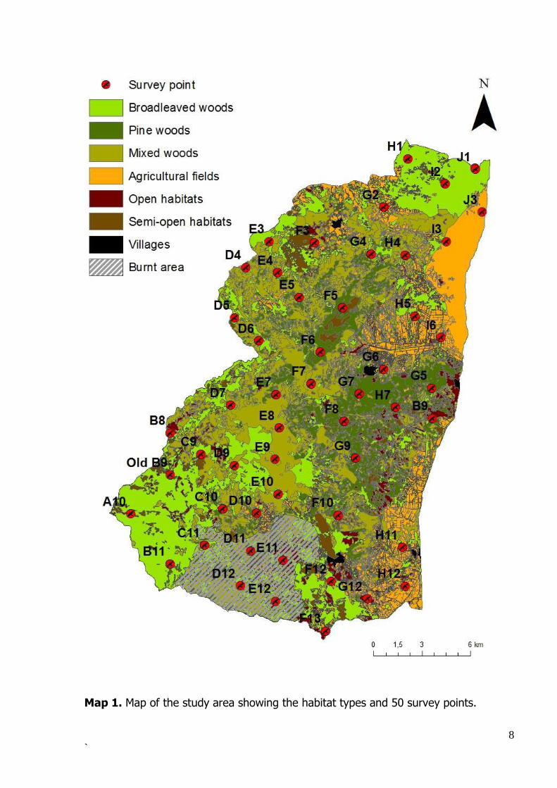
The Dadia-Lefkimi-Soufli Forest National Park is situated in the Evros Prefecture, Northeastern Greece (Map 1). It consists of a forest complex that extends over 43.000 ha (hereafter called the study area) including two zones of strict protection (core areas), which cover a total of 7.250 ha. The study area is characterized by gently sloping valleys covered by oak (Quercus frainetto, Q. cerris, Q. pubescens) and pine (Pinus brutia and P. nigra) forests and includes a variety of other habitats such as fields, pastures, torrents and rocky outcrops (Adamakopoulos et al., 1995). A change in the habitat coverage of the National Park was caused by a large forest fire that occurred in 2011. It affected the south-central part of the area and burned 6200 ha, of which 63.22% (3920 ha) were within the limits of the DNP (WWF Greece, 2011).

The Dadia- Lefkimi- Soufli Forest National Park is acknowledged for its high

ornithological interest, as it is used for nesting, wintering and passage by a wide diversity of birds of prey (Poirazidis et al., 1996; Poirazidis et al., 2011). In total, out

7

`

of the 39 raptor species occurring in Europe, 36 have been observed in the area. It is unique because the area hosts the last breeding population in the Balkans of the Black Vulture (Aegypius monachus) (Skartsi et al., 2010). It is also considered to be the last stronghold of the Egyptian Vulture (Neophron percnopterus) in the country, a species that recently has declined dramatically (Kret, 2011). The populations of other bird of prey species are very large in the reserve and comprise important parts of their populations in Greece. Examples include the Lesser Spotted Eagle (Aquila pomarina), the Booted Eagle (Aquila pennata) and the Short-toed Eagle (Circaetus gallicus) (Ruiz & Pomarède, 2012).

The study was carried out between January 2012 and March 2013. We

searched for the following six species that occurred and bred in the study area: Barn Owl (Tyto alba), Eurasian Eagle Owl (Bubo bubo), Eurasian Scops Owl (Otus scops), Little Owl (Athene noctua), Long-eared Owl (Asio otus) and Tawny Owl (Strix aluco) (Catsadorakis & Kallander, 2010).

2.2. Survey points

In order to obtain a representative sample of all habitats that occur in DNP, the

study area was divided into a grid of 78 equal squares (2.5 x 2.5 km). The percentage of different habitats in each square was calculated and for simplicity up to three habitat categories were assigned to each square. Based on the appropriate habitat type, 50 survey points were selected randomly using a stratified random design, filtered additionally by road accessibility and avoidance of the bottom of valleys and the top of hills (Table 1 & Map 1). Villages were excluded from the study area due to logistic reasons and because they require different survey methods.

Table 1. Habitat categories and the number of survey points

Habitat Surface (ha) Percentage Number of survey

points

Broad-leaved woods

11577 26.7 13

Agricultural fields 6816 15.7 8

Open habitats 1586 3.7 2

Pine woods 5360 12.4 6

Semi-open habitats

2036 4.7 2

Mixed woods 11756 27.2 14

Burnt area 4016 9.3 5

8

`

Map 1. Map of the study area showing the habitat types and 50 survey points.

9

`

2.3. Field survey

Territorial individuals were detected by means of their vocalizations, occurring either spontaneously or as a response to a playback call that simulates a territorial intrusion. For each survey point data collection was divided into three main phases (Martínez & Zuberogoita, 2002):

1. Spontaneous calls (SC). At the beginning of each census a period of silence

was maintained in order to detect spontaneous calls.

2. Playback calls (PBC). Recorded calls of territorial males were broadcast to

simulate a territorial intrusion and to provoke an answer by any territorial

individuals. In the 2nd survey, where more than one species was recorded, the

sequence of vocalization followed that of an increasing owl species size in order

to minimize the disturbance caused by other owl species leading to inter-

specific competition and predation (Mikkola, 1983).

3. Post playback period (PPP). At the end of the census a final period of silence

was kept. This final period of silence was done to detect individuals that may

become active vocally after a potential owl intruder leaves the area.

Survey equipment included an mp³ player, a GPS receiver, a torch and a compass. The following data were recorded prior to the onset of survey activities at every survey point (Appendix I):

Observers‟ names Start and end time

Temperature Survey point number Habitat code

When an individual owl was detected the following data were collected:

Species Sex (when possible)

Time of the first calling in the different census phases (SC, PBC and PPP) Visual contact Direction from which the bird calls originate Comments

Collected data were stored in a database for use with the GIS software in order to be analysed subsequently.

Because reproductive period differed from species to species and in order to

survey the period of highest calling activity for each species three different surveys were completed.

10

`

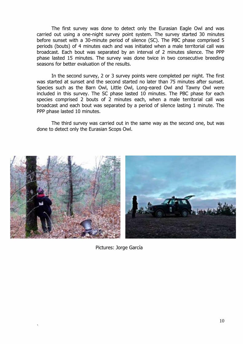
The first survey was done to detect only the Eurasian Eagle Owl and was carried out using a one-night survey point system. The survey started 30 minutes before sunset with a 30-minute period of silence (SC). The PBC phase comprised 5 periods (bouts) of 4 minutes each and was initiated when a male territorial call was broadcast. Each bout was separated by an interval of 2 minutes silence. The PPP phase lasted 15 minutes. The survey was done twice in two consecutive breeding seasons for better evaluation of the results.

In the second survey, 2 or 3 survey points were completed per night. The first was started at sunset and the second started no later than 75 minutes after sunset. Species such as the Barn Owl, Little Owl, Long-eared Owl and Tawny Owl were included in this survey. The SC phase lasted 10 minutes. The PBC phase for each species comprised 2 bouts of 2 minutes each, when a male territorial call was broadcast and each bout was separated by a period of silence lasting 1 minute. The PPP phase lasted 10 minutes.

The third survey was carried out in the same way as the second one, but was done to detect only the Eurasian Scops Owl.

Pictures: Jorge García

11

`

2.4. Habitat suitability modeling

Species distribution models (SDMs) based on presence-only occurrence data have been widely used in the last few decades to model ecological niches, to investigate biogeographical distributions as well as for conservation planning (Hirzel et al., 2002; Phillips et al., 2006; Peterson et al., 2011). In this report we analyzed the potential distribution of each owl species based on the station vocalization data using the software Maxent (Phillips et al., 2006). We chose Maxent v.3.3 as it is a commonly used modelling software and it has been found to perform well for (a) small sample sizes and noisy data (Shcheglovitova & Anderson, 2013); (b) categorical data and (c) modelling interactions (Phillips et al., 2006).

We modelled the distribution of owls using 24 environmental variables

representing topography, landscape features and disturbance (Table 2). For topographic features (12 variables) a digital terrain model with a resolution of ~ 27 m (Aster GDEM) was used and rescaled to 30m. The derived topographic variables (mean altitude, % slope, hill shade and standard deviation of the elevation) were calculated within a moving window of radius 250m and 500m. A Topographic Position Index was initially classified into either three or five classes (using natural break intervals) to represent the lowest, middle and upper regions of the landscape. The majority of the classes were calculated using the previously mentioned circles of 250m and 500m. Modelling was done at these two spatial scales (250m and 500m) to determine whether different factors operate at different scales. The scales were chosen based on the average distances over which it is possible for the owls to be heard by observers.

Landscape was represented by seven variables. A contemporaneously acquired

Landsat 8 image (28 July 2013) was used to create a forest-cover mask by classification using supervised algorithms (Maxlike). All forest types were classified as forest region and all open habitats (agricultural zone, forest openings) as open region. Both regions were merged in a binary image (0,1) and the percentage of forest cover was calculated at scales of 250m and 500m. A 300 x 300 m grid was overlaid on a high-resolution satellite image of the area and the presence of mature trees was determined using a visual 7th scale ordinal estimation, where 0 = no mature trees and 6 = maximum coverage of the square by mature trees. In the analysis, this variable was used both as categorical data as well as the percentage presence of mature trees at both spatial scales (250m and 500m). In this case all the squares scored with a 0 value were reclassified as "0" and all the squares scored with values of 1-6 were reclassified as "1". The landscape structure was represented by two Principal Component Factors to characterise the diversity and fragmentation of habitats respectively and these were based on a previous specific study of the area (Schindler et al., 2008). The hexagons of the initial study (Schindler et al., 2008) were first reformatted to be point features and secondly were interpolated in the study area using an Inverse Weighted Analysis.

Five variables based on distance characteristics were used in this study. The

first three (main streams, all streams and rocky sites) represented ecological features of the habitats and the last two (distance to known Eurasian Eagle Owl nests and

12

`

distance to the nearest urban location) represented potential disturbance characteristics for the owl species.

All datasets were transformed to the Greek Geodetic Reference System. Table 2. The variables used in the habitat suitability models

To avoid over-fitting of the models, only one variable of scale (250m or 500m)

was used in the final analysis for each species. The variable was selected using a Jackknife test based on a very low added „cumulative gain‟ in preliminary Maxent runs to indicate its relative importance. Further reduction of the datasets was avoided as correlations are frequent in ecology and essential information might thus accidentally be discarded in the process (Burnam & Anderson, 1998).

Variable Description

Topographical

Elevation (m) Calculated at two spatial scales: 250m and 500m

Slope (%) Calculated at two spatial scales: 250m and 500m

Hillshade (0-255) Calculated at two spatial scales: 250m and 500m

SDDem Standard Deviation of Elevation (measure of topographic

roughness) = “(meanDEM” – “DEM”) / “rangeDEM”, calculated at two spatial scales: 250m and 500m

Topo_index Topographic Position Index (terrain ruggedness metric and

a local elevation index) = (“DEM″ – “minDEM”) / (“maxDEM” – “minDEM”), rescaled in 3 categories and in 5

categories, both calculated at two spatial scales: 250m and 500m

Landscape

Forest2013 Forest coverage (%), including all types of forest in Landsat image (July 2013) calculated at two spatial scales:

250m and 500m

old forest Categorical variable in 7 classes representing the amount

of old (mature) forest in squares of 300 m (0=no old forest

and 6=maximum)

land factor 1 Principal component factor representing the diversity of

Dadia landscape (Schindler at al. 2008)

land factor 2 Principal component factor representing the fragmentation of Dadia landscape (Schindler at al. 2008)

Distance

dst_rocks Distance to the nearest rocky area

dst_main streams Distance to the nearest main stream

dst_streams Distance to the nearest stream

dst_urban Distance to the nearest urban area

dst_bubo bubo Distance to the nearest Eurasian Eagle Owl nest (used for

all species, except the Eurasian Eagle Owl)

13

`

We followed the default setting parameters of the software (e.g. 10,000 randomly chosen background pixels from the predictor grids), but we checked for model over-fitting by calculating three values of the regularization. This tool reduces the iterative gain and helps to avoid over-fitting of the model especially if few presence records are available. A higher regularization value leads to a wider predicted distribution. By "default" the software used the value of 1, but in this study we also analysed the model effect by using regularization values of "0.75" and "1.5". The relative importance of each predictor was determined by the Jackknife method, and the threshold-independent Receiver Operator Characteristic (ROC) was employed because it yielded the Area Under Curve (AUC) value as a single indicator of model performance (Hirzel & Guisan, 2002; Phillips et al., 2006). Response Curves of the most important variables were also calculated in order to understand the effect of this variable on the probability of species occurence.

14

`

3. RESULTS

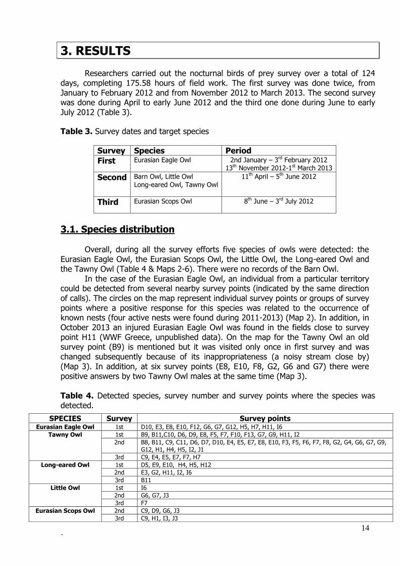
Researchers carried out the nocturnal birds of prey survey over a total of 124 days, completing 175.58 hours of field work. The first survey was done twice, from January to February 2012 and from November 2012 to March 2013. The second survey was done during April to early June 2012 and the third one done during June to early July 2012 (Table 3).

Table 3. Survey dates and target species

Survey Species Period

First Eurasian Eagle Owl 2nd January – 3rd February 2012 13th November 2012-1st March 2013

Second Barn Owl, Little Owl

Long-eared Owl, Tawny Owl

11th April – 5th June 2012

Third Eurasian Scops Owl 8th June – 3rd July 2012

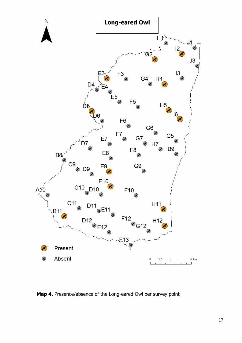
3.1. Species distribution Overall, during all the survey efforts five species of owls were detected: the

Eurasian Eagle Owl, the Eurasian Scops Owl, the Little Owl, the Long-eared Owl and the Tawny Owl (Table 4 & Maps 2-6). There were no records of the Barn Owl.

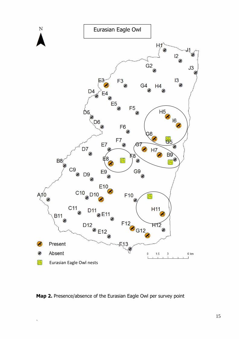
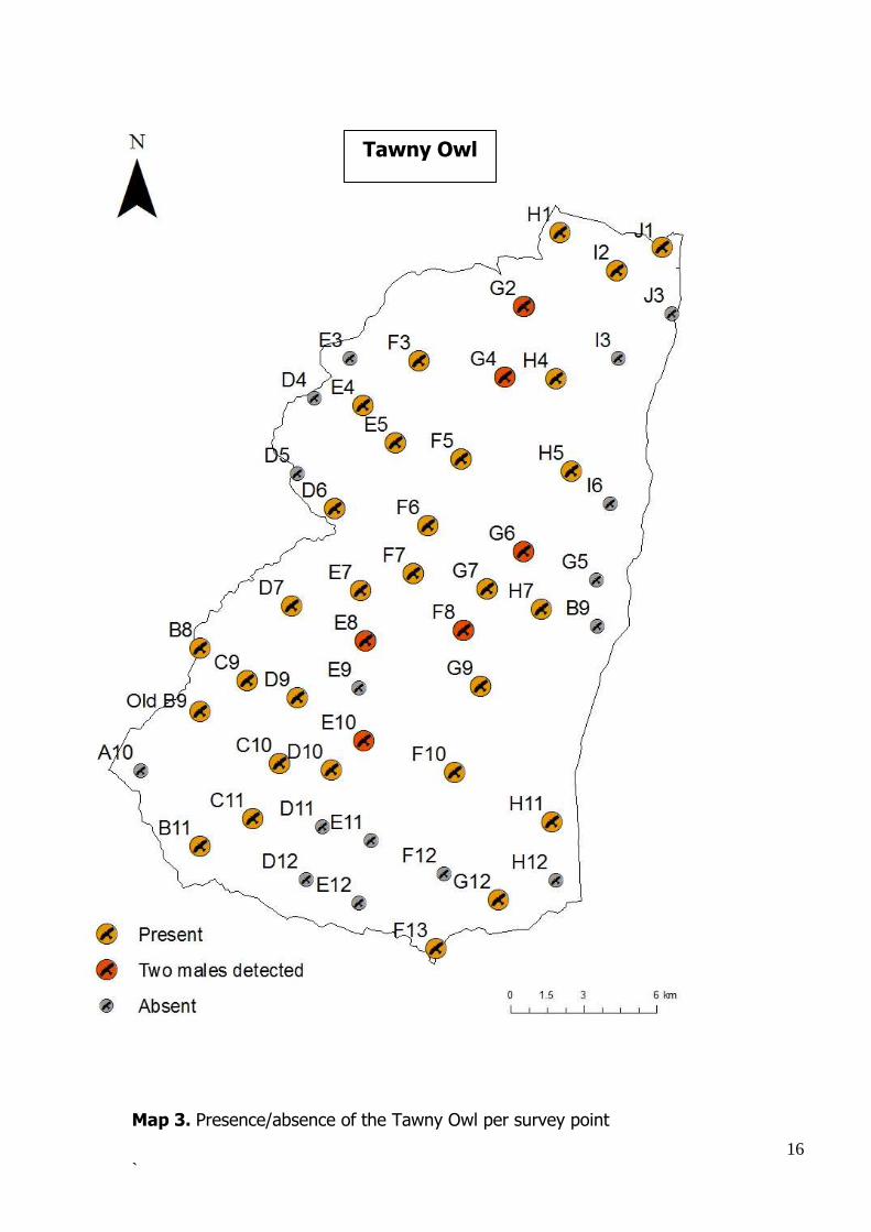
In the case of the Eurasian Eagle Owl, an individual from a particular territory could be detected from several nearby survey points (indicated by the same direction of calls). The circles on the map represent individual survey points or groups of survey points where a positive response for this species was related to the occurrence of known nests (four active nests were found during 2011-2013) (Map 2). In addition, in October 2013 an injured Eurasian Eagle Owl was found in the fields close to survey point H11 (WWF Greece, unpublished data). On the map for the Tawny Owl an old survey point (B9) is mentioned but it was visited only once in first survey and was changed subsequently because of its inappropriateness (a noisy stream close by) (Map 3). In addition, at six survey points (E8, E10, F8, G2, G6 and G7) there were positive answers by two Tawny Owl males at the same time (Map 3).

Table 4. Detected species, survey number and survey points where the species was detected.

SPECIES Survey Survey points Eurasian Eagle Owl 1st D10, E3, E8, E10, F12, G6, G7, G12, H5, H7, H11, I6

Tawny Owl

1st B9, B11,C10, D6, D9, E8, F5, F7, F10, F13, G7, G9, H11, I2

2nd B8, B11, C9, C11, D6, D7, D10, E4, E5, E7, E8, E10, F3, F5, F6, F7, F8, G2, G4, G6, G7, G9, G12, H1, H4, H5, I2, J1

3rd C9, E4, E5, E7, F7, H7

Long-eared Owl

1st D5, E9, E10, H4, H5, H12

2nd E3, G2, H11, I2, I6

3rd B11

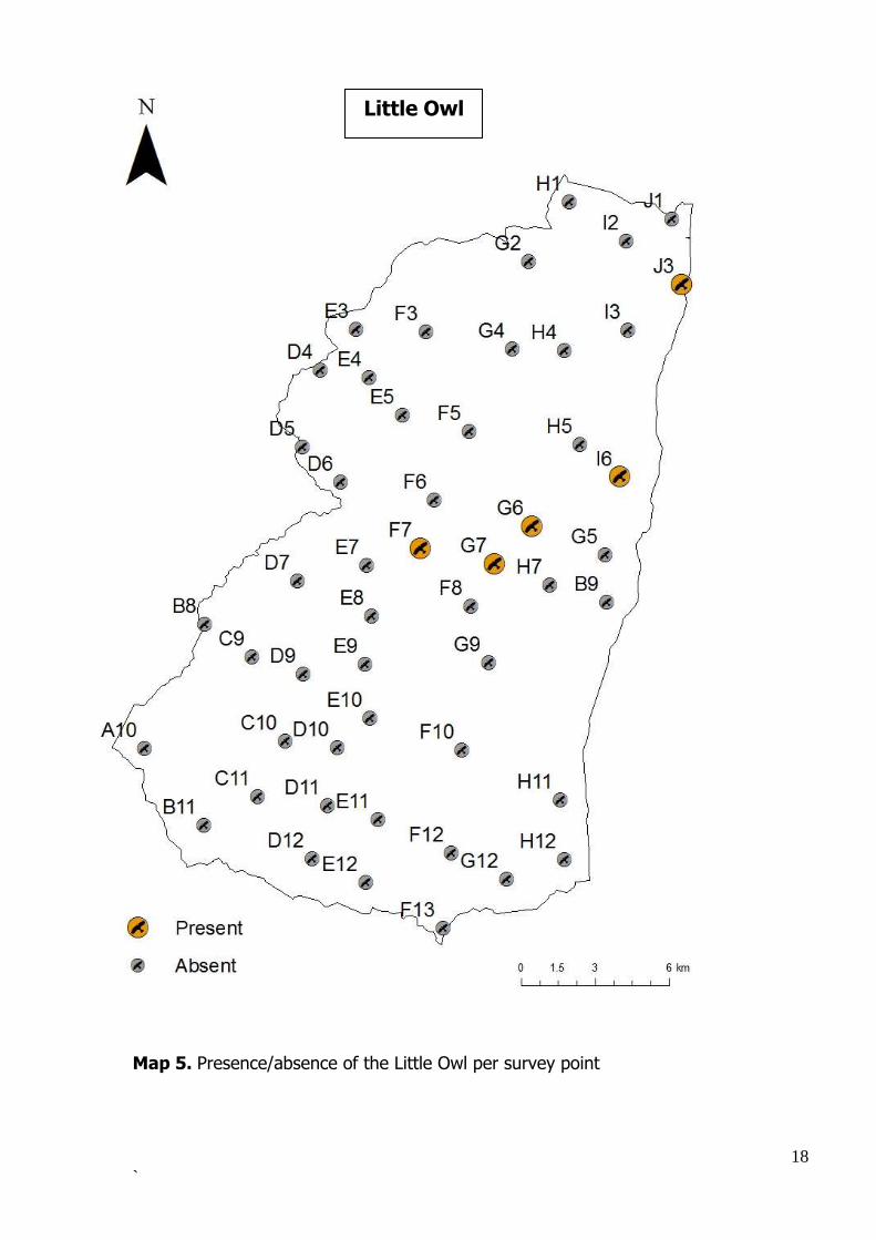
Little Owl

1st I6

2nd G6, G7, J3

3rd F7

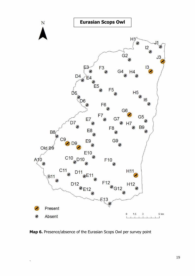
Eurasian Scops Owl

2nd C9, D9, G6, J3

3rd C9, H1, I3, J3

15

`

Map 2. Presence/absence of the Eurasian Eagle Owl per survey point

Eurasian Eagle Owl

Eurasian Eagle Owl nests

16

`

Map 3. Presence/absence of the Tawny Owl per survey point

Tawny Owl

17

`

Map 4. Presence/absence of the Long-eared Owl per survey point

Long-eared Owl

18

`

Map 5. Presence/absence of the Little Owl per survey point

Little Owl

19

`

Map 6. Presence/absence of the Eurasian Scops Owl per survey point

Eurasian Scops Owl

20

`

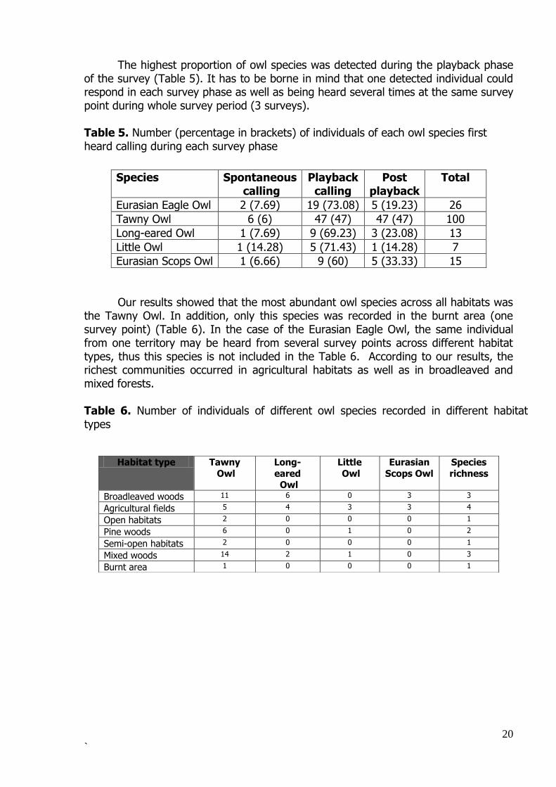
The highest proportion of owl species was detected during the playback phase of the survey (Table 5). It has to be borne in mind that one detected individual could respond in each survey phase as well as being heard several times at the same survey point during whole survey period (3 surveys). Table 5. Number (percentage in brackets) of individuals of each owl species first heard calling during each survey phase

Species Spontaneous

calling Playback

calling Post

playback Total

Eurasian Eagle Owl 2 (7.69) 19 (73.08) 5 (19.23) 26

Tawny Owl 6 (6) 47 (47) 47 (47) 100

Long-eared Owl 1 (7.69) 9 (69.23) 3 (23.08) 13

Little Owl 1 (14.28) 5 (71.43) 1 (14.28) 7

Eurasian Scops Owl 1 (6.66) 9 (60) 5 (33.33) 15

Our results showed that the most abundant owl species across all habitats was

the Tawny Owl. In addition, only this species was recorded in the burnt area (one survey point) (Table 6). In the case of the Eurasian Eagle Owl, the same individual from one territory may be heard from several survey points across different habitat types, thus this species is not included in the Table 6. According to our results, the richest communities occurred in agricultural habitats as well as in broadleaved and mixed forests. Table 6. Number of individuals of different owl species recorded in different habitat types

Habitat type Tawny

Owl

Long-

eared Owl

Little

Owl

Eurasian

Scops Owl

Species

richness

Broadleaved woods 11 6 0 3 3

Agricultural fields 5 4 3 3 4

Open habitats 2 0 0 0 1

Pine woods 6 0 1 0 2

Semi-open habitats 2 0 0 0 1

Mixed woods 14 2 1 0 3

Burnt area 1 0 0 0 1

21

`

3.2. Habitat suitability modeling

3.2.1. Evaluation of the models

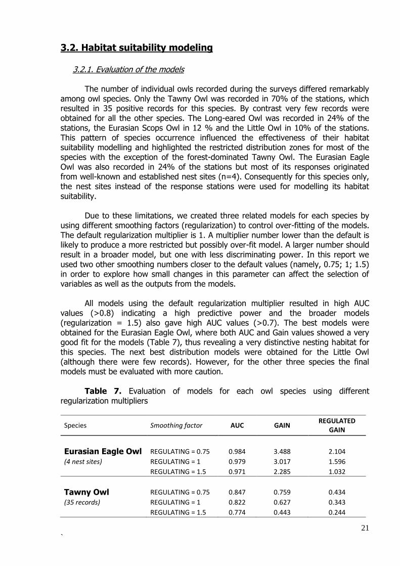
The number of individual owls recorded during the surveys differed remarkably among owl species. Only the Tawny Owl was recorded in 70% of the stations, which resulted in 35 positive records for this species. By contrast very few records were obtained for all the other species. The Long-eared Owl was recorded in 24% of the stations, the Eurasian Scops Owl in 12 % and the Little Owl in 10% of the stations. This pattern of species occurrence influenced the effectiveness of their habitat suitability modelling and highlighted the restricted distribution zones for most of the species with the exception of the forest-dominated Tawny Owl. The Eurasian Eagle Owl was also recorded in 24% of the stations but most of its responses originated from well-known and established nest sites (n=4). Consequently for this species only, the nest sites instead of the response stations were used for modelling its habitat suitability.

Due to these limitations, we created three related models for each species by

using different smoothing factors (regularization) to control over-fitting of the models. The default regularization multiplier is 1. A multiplier number lower than the default is likely to produce a more restricted but possibly over-fit model. A larger number should result in a broader model, but one with less discriminating power. In this report we used two other smoothing numbers closer to the default values (namely, 0.75; 1; 1.5) in order to explore how small changes in this parameter can affect the selection of variables as well as the outputs from the models.

All models using the default regularization multiplier resulted in high AUC values (>0.8) indicating a high predictive power and the broader models (regularization = 1.5) also gave high AUC values (>0.7). The best models were obtained for the Eurasian Eagle Owl, where both AUC and Gain values showed a very good fit for the models (Table 7), thus revealing a very distinctive nesting habitat for this species. The next best distribution models were obtained for the Little Owl (although there were few records). However, for the other three species the final models must be evaluated with more caution.

Table 7. Evaluation of models for each owl species using different

regularization multipliers

Species Smoothing factor AUC GAIN REGULATED

GAIN

Eurasian Eagle Owl REGULATING = 0.75 0.984 3.488 2.104

(4 nest sites) REGULATING = 1 0.979 3.017 1.596

REGULATING = 1.5 0.971 2.285 1.032

Tawny Owl REGULATING = 0.75 0.847 0.759 0.434

(35 records) REGULATING = 1 0.822 0.627 0.343

REGULATING = 1.5 0.774 0.443 0.244

22

`

Long-eared Owl REGULATING = 0.75 0.813 0.666 0.407

(12 records) REGULATING = 1 0.809 0.611 0.329

REGULATING = 1.5 0.785 0.483 0.214

Eurasian Scops Owl REGULATING = 0.75 0.829 0.799 0.47

(6 records) REGULATING = 1 0.806 0.73 0.37

REGULATING = 1.5 0.799 0.601 0.217

Little Owl REGULATING = 0.75 0.938 1.27 0.671

(5 records) REGULATING = 1 0.915 0.971 0.521

REGULATING = 1.5 0.867 0.712 0.361

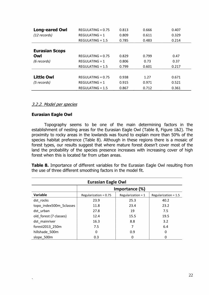
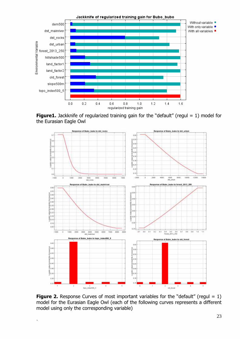
3.2.2. Model per species Eurasian Eagle Owl

Topography seems to be one of the main determining factors in the establishment of nesting areas for the Eurasian Eagle Owl (Table 8, Figure 1&2). The proximity to rocky areas in the lowlands was found to explain more than 50% of the species habitat preference (Table 8). Although in these regions there is a mosaic of forest types, our results suggest that where mature forest doesn‟t cover most of the land the probability of the species presence increases with increasing cover of high forest when this is located far from urban areas. Table 8. Importance of different variables for the Eurasian Eagle Owl resulting from the use of three different smoothing factors in the model fit.

Eurasian Eagle Owl

Importance (%) Variable Regularization = 0.75 Regularization = 1 Regularization = 1.5

dst_rocks 23.9 25.3 40.2

topo_index500m_5classes 11.8 23.4 23.2

dst_urban 27.8 19 7.5

old_forest (7 classes) 12.4 15.5 19.5

dst_mainriver 16.3 8.8 3.2

forest2013_250m 7.5 7 6.4

hillshade_500m 0 0.9 0

slope_500m 0.3 0 0

23

`

Figure1. Jackknife of regularized training gain for the “default” (regul = 1) model for the Eurasian Eagle Owl Figure 2. Response Curves of most important variables for the “default” (regul = 1) model for the Eurasian Eagle Owl (each of the following curves represents a different model using only the corresponding variable)

24

`

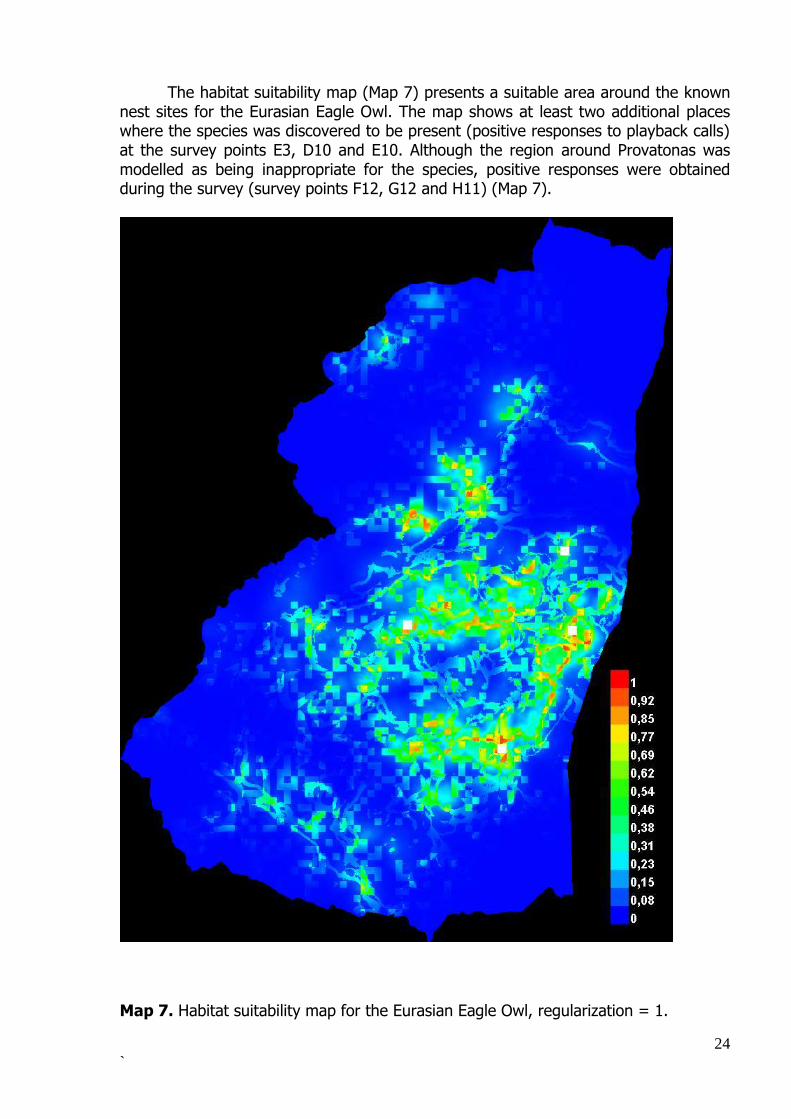
The habitat suitability map (Map 7) presents a suitable area around the known nest sites for the Eurasian Eagle Owl. The map shows at least two additional places where the species was discovered to be present (positive responses to playback calls) at the survey points E3, D10 and E10. Although the region around Provatonas was modelled as being inappropriate for the species, positive responses were obtained during the survey (survey points F12, G12 and H11) (Map 7).

Map 7. Habitat suitability map for the Eurasian Eagle Owl, regularization = 1.

25

`

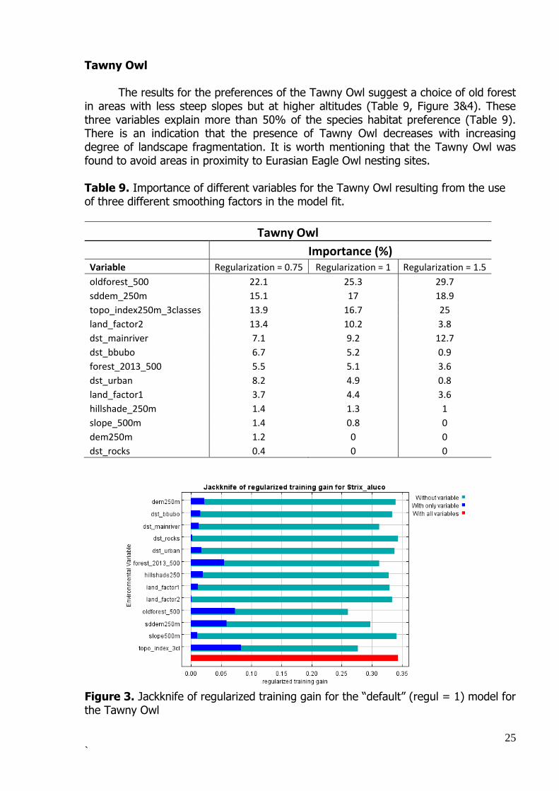
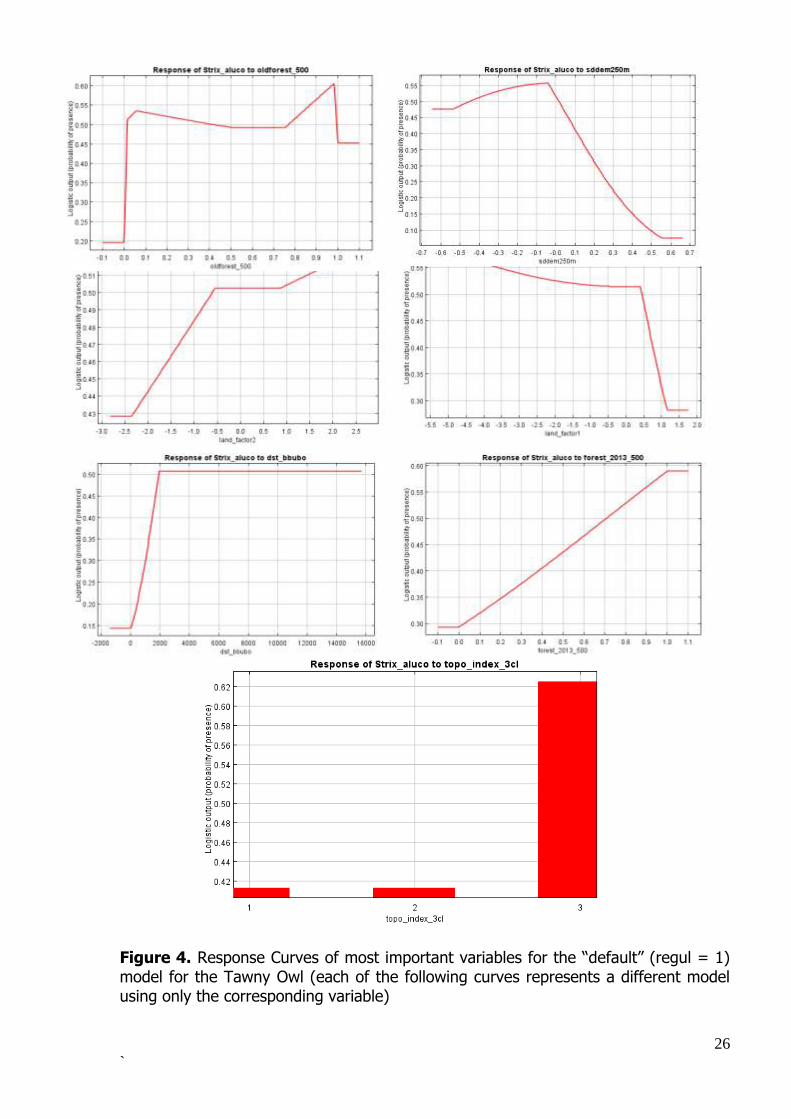
Tawny Owl

The results for the preferences of the Tawny Owl suggest a choice of old forest in areas with less steep slopes but at higher altitudes (Table 9, Figure 3&4). These three variables explain more than 50% of the species habitat preference (Table 9). There is an indication that the presence of Tawny Owl decreases with increasing degree of landscape fragmentation. It is worth mentioning that the Tawny Owl was found to avoid areas in proximity to Eurasian Eagle Owl nesting sites. Table 9. Importance of different variables for the Tawny Owl resulting from the use of three different smoothing factors in the model fit.

Tawny Owl

Importance (%) Variable Regularization = 0.75 Regularization = 1 Regularization = 1.5

oldforest_500 22.1 25.3 29.7

sddem_250m 15.1 17 18.9

topo_index250m_3classes 13.9 16.7 25

land_factor2 13.4 10.2 3.8

dst_mainriver 7.1 9.2 12.7

dst_bbubo 6.7 5.2 0.9

forest_2013_500 5.5 5.1 3.6

dst_urban 8.2 4.9 0.8

land_factor1 3.7 4.4 3.6

hillshade_250m 1.4 1.3 1

slope_500m 1.4 0.8 0

dem250m 1.2 0 0

dst_rocks 0.4 0 0

Figure 3. Jackknife of regularized training gain for the “default” (regul = 1) model for the Tawny Owl

26

`

0

0 0251690496

Figure 4. Response Curves of most important variables for the “default” (regul = 1) model for the Tawny Owl (each of the following curves represents a different model using only the corresponding variable)

27

`

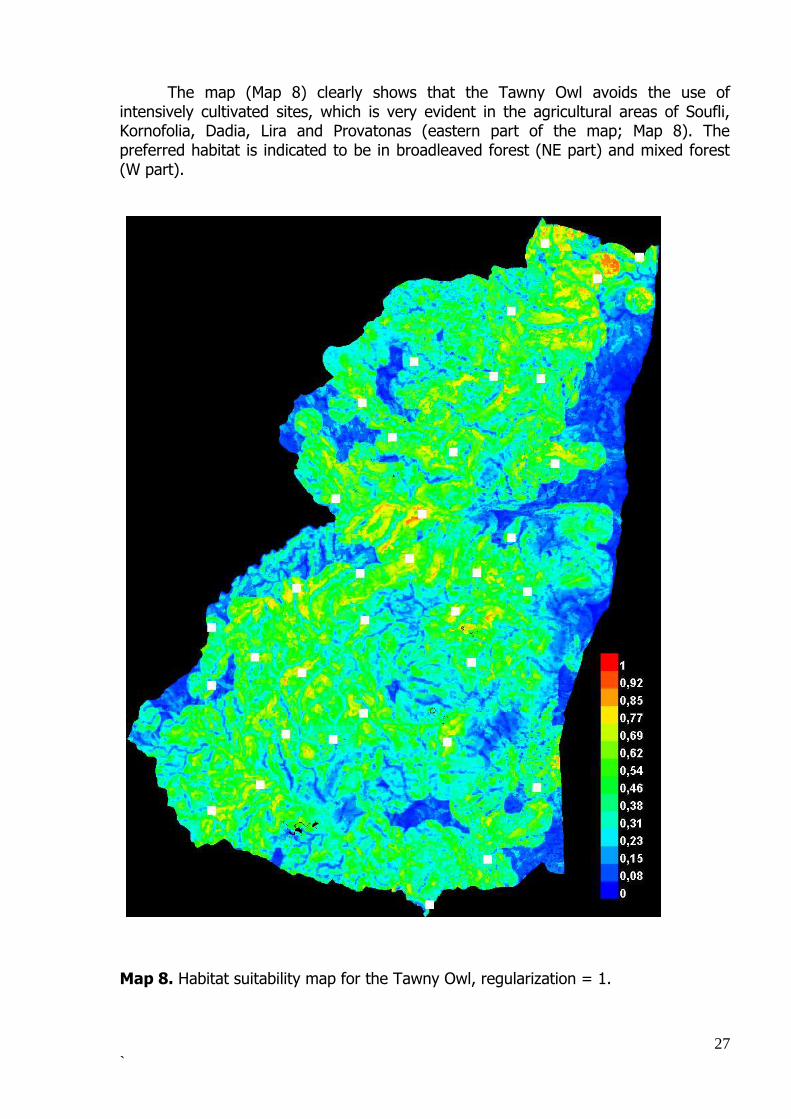
The map (Map 8) clearly shows that the Tawny Owl avoids the use of intensively cultivated sites, which is very evident in the agricultural areas of Soufli, Kornofolia, Dadia, Lira and Provatonas (eastern part of the map; Map 8). The preferred habitat is indicated to be in broadleaved forest (NE part) and mixed forest (W part). Map 8. Habitat suitability map for the Tawny Owl, regularization = 1.

28

`

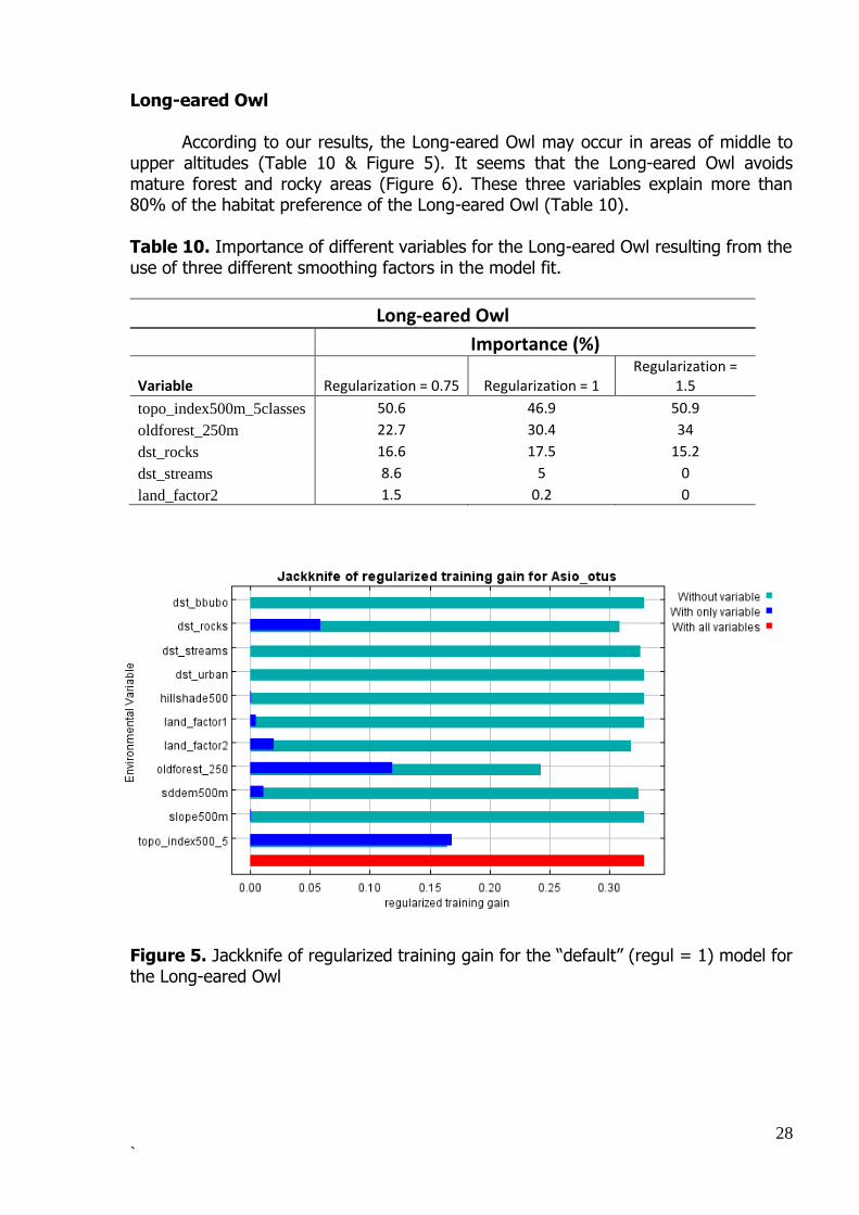
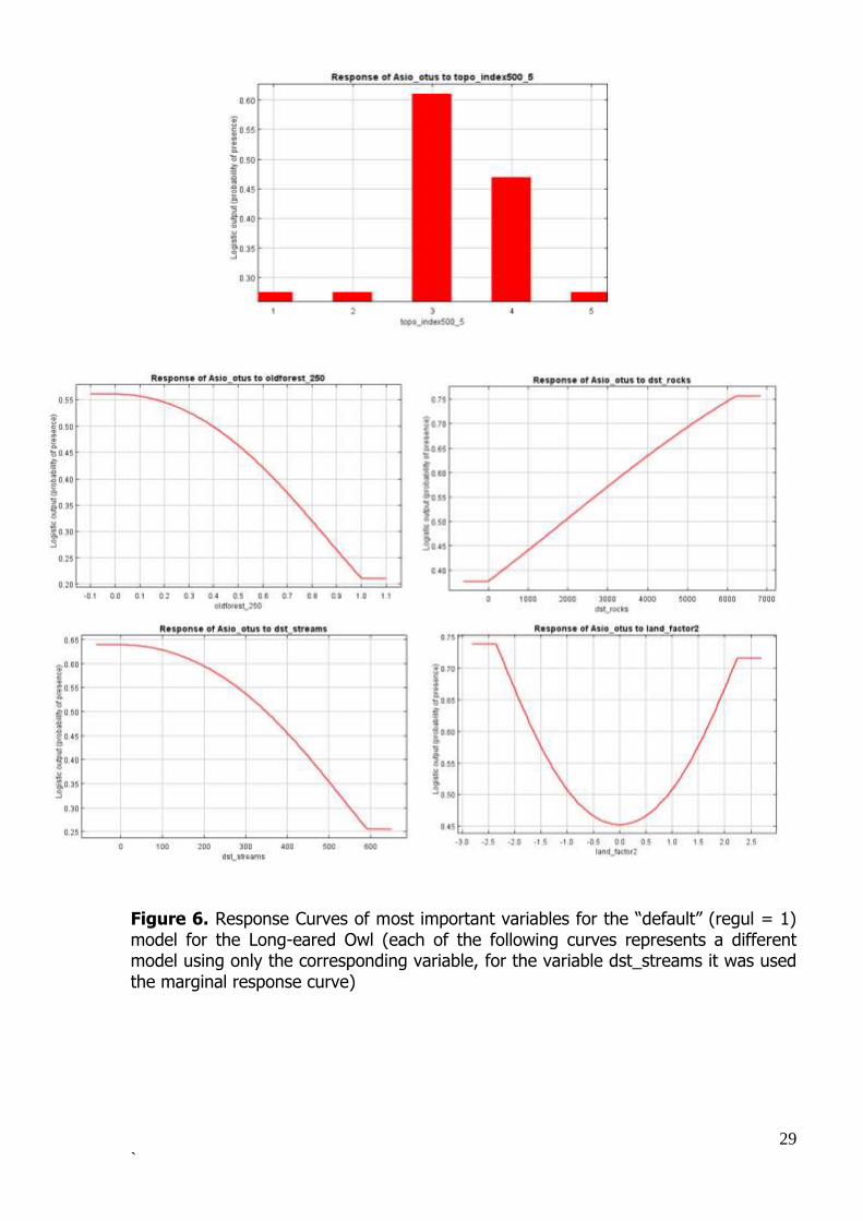
Long-eared Owl

According to our results, the Long-eared Owl may occur in areas of middle to upper altitudes (Table 10 & Figure 5). It seems that the Long-eared Owl avoids mature forest and rocky areas (Figure 6). These three variables explain more than 80% of the habitat preference of the Long-eared Owl (Table 10). Table 10. Importance of different variables for the Long-eared Owl resulting from the use of three different smoothing factors in the model fit.

Long-eared Owl

Importance (%)

Variable Regularization = 0.75 Regularization = 1 Regularization =

1.5

topo_index500m_5classes 50.6 46.9 50.9

oldforest_250m 22.7 30.4 34

dst_rocks 16.6 17.5 15.2

dst_streams 8.6 5 0

land_factor2 1.5 0.2 0

Figure 5. Jackknife of regularized training gain for the “default” (regul = 1) model for the Long-eared Owl

29

`

0

0

Figure 6. Response Curves of most important variables for the “default” (regul = 1) model for the Long-eared Owl (each of the following curves represents a different model using only the corresponding variable, for the variable dst_streams it was used the marginal response curve)

30

`

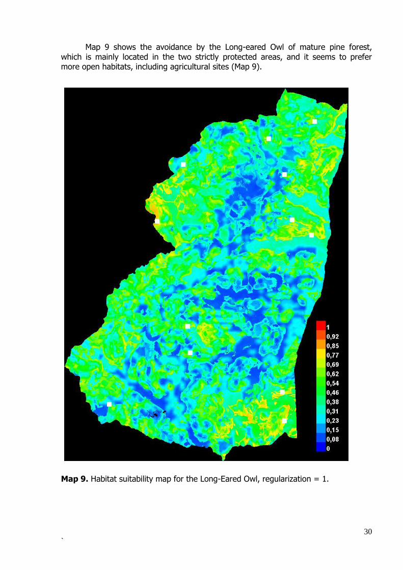
Map 9 shows the avoidance by the Long-eared Owl of mature pine forest, which is mainly located in the two strictly protected areas, and it seems to prefer more open habitats, including agricultural sites (Map 9). Map 9. Habitat suitability map for the Long-Eared Owl, regularization = 1.

31

`

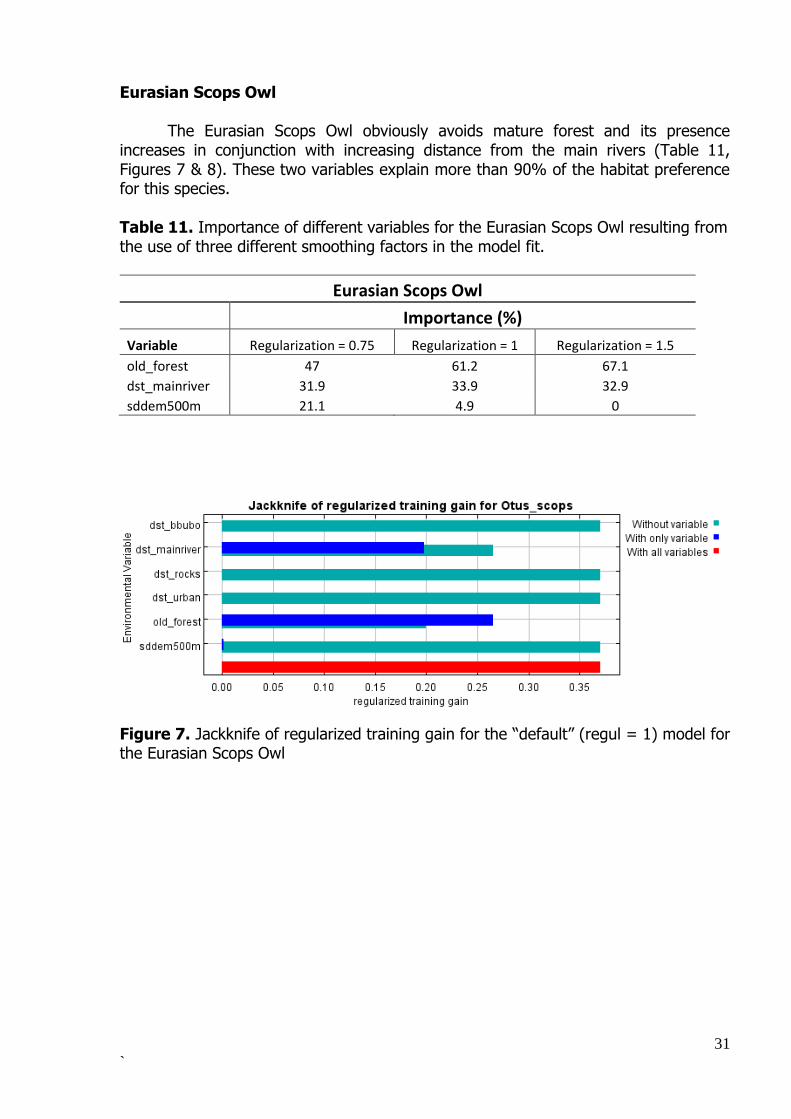
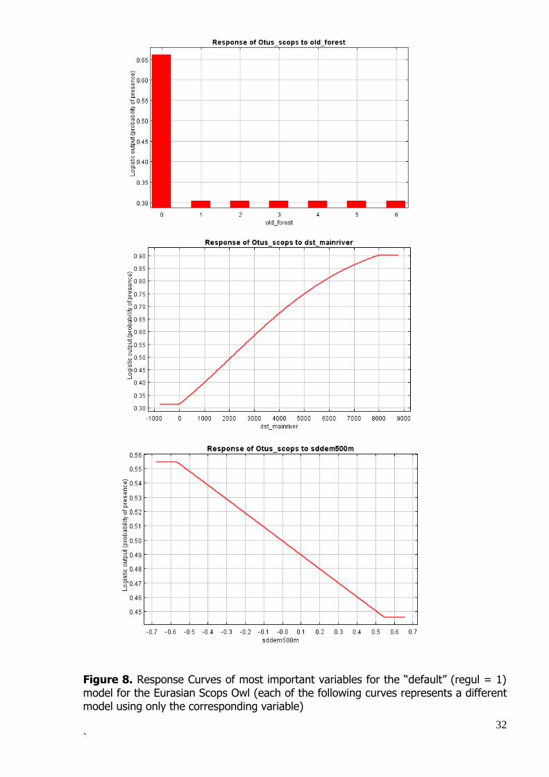
Eurasian Scops Owl The Eurasian Scops Owl obviously avoids mature forest and its presence increases in conjunction with increasing distance from the main rivers (Table 11, Figures 7 & 8). These two variables explain more than 90% of the habitat preference for this species. Table 11. Importance of different variables for the Eurasian Scops Owl resulting from the use of three different smoothing factors in the model fit.

Eurasian Scops Owl

Importance (%)

Variable Regularization = 0.75 Regularization = 1 Regularization = 1.5

old_forest 47 61.2 67.1

dst_mainriver 31.9 33.9 32.9

sddem500m 21.1 4.9 0

Figure 7. Jackknife of regularized training gain for the “default” (regul = 1) model for the Eurasian Scops Owl

32

`

Figure 8. Response Curves of most important variables for the “default” (regul = 1) model for the Eurasian Scops Owl (each of the following curves represents a different model using only the corresponding variable)

33

`

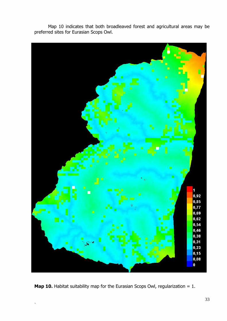
Map 10 indicates that both broadleaved forest and agricultural areas may be preferred sites for Eurasian Scops Owl. Map 10 Habitat suitability map of the Long-eared owl, regularization = 1. Map 10. Habitat suitability map for the Eurasian Scops Owl, regularization = 1.

34

`

Little Owl

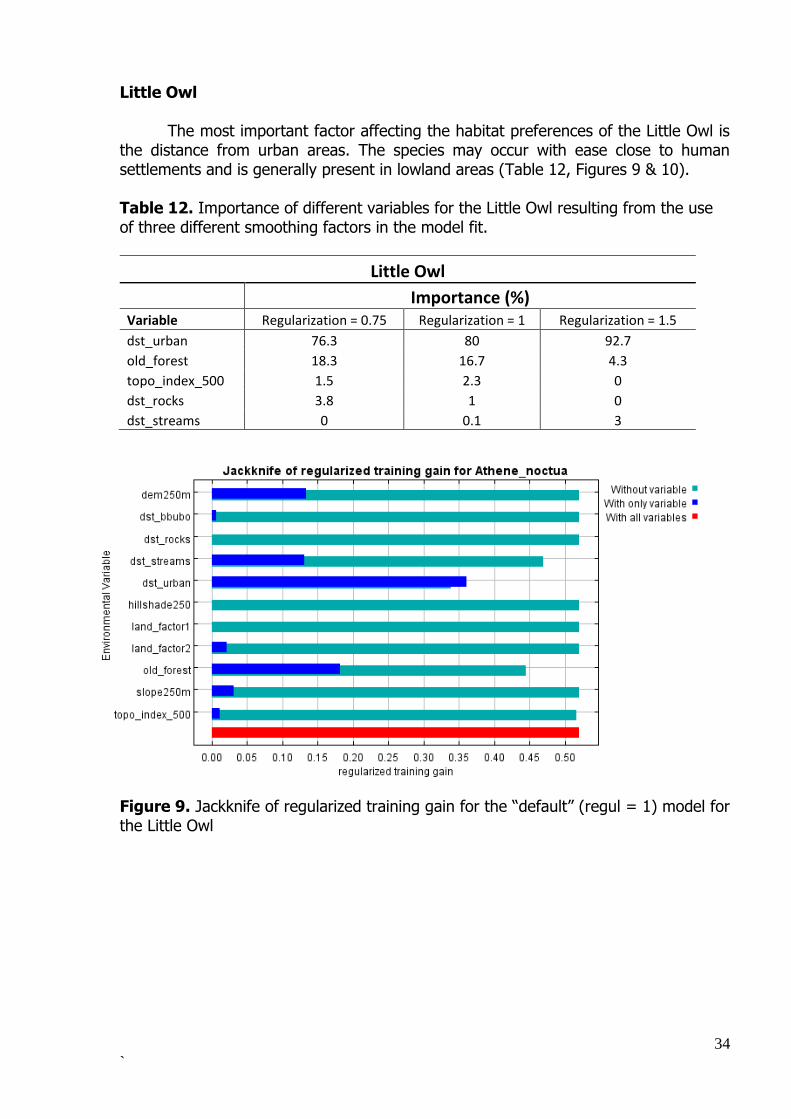
The most important factor affecting the habitat preferences of the Little Owl is the distance from urban areas. The species may occur with ease close to human settlements and is generally present in lowland areas (Table 12, Figures 9 & 10). Table 12. Importance of different variables for the Little Owl resulting from the use of three different smoothing factors in the model fit.

Little Owl

Importance (%) Variable Regularization = 0.75 Regularization = 1 Regularization = 1.5

dst_urban 76.3 80 92.7

old_forest 18.3 16.7 4.3

topo_index_500 1.5 2.3 0

dst_rocks 3.8 1 0

dst_streams 0 0.1 3

Figure 9. Jackknife of regularized training gain for the “default” (regul = 1) model for the Little Owl

35

`

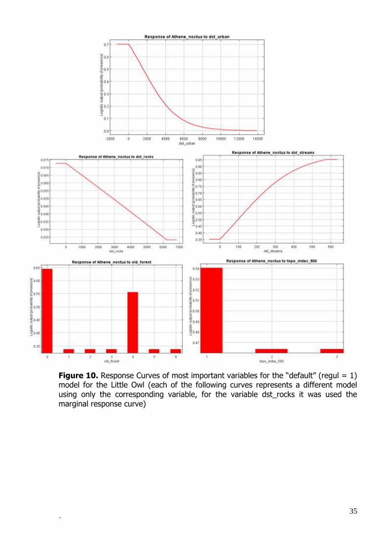
Figure 10. Response Curves of most important variables for the “default” (regul = 1) model for the Little Owl (each of the following curves represents a different model using only the corresponding variable, for the variable dst_rocks it was used the marginal response curve)

36

`

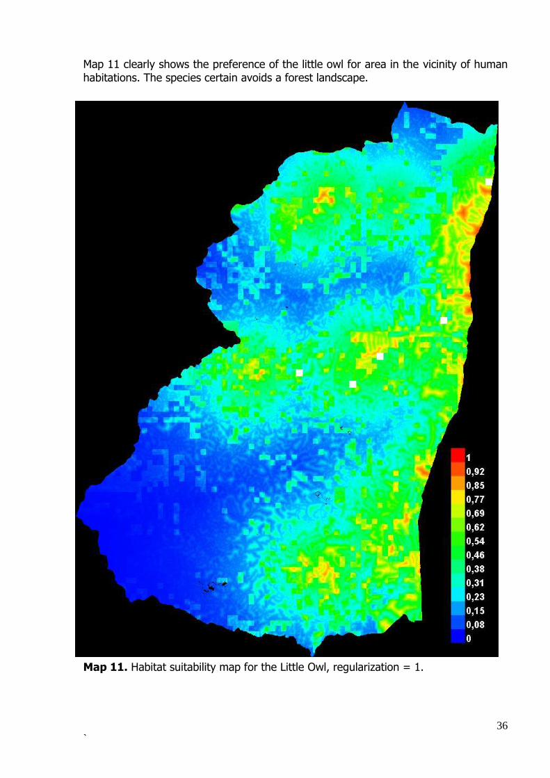
Map 11 clearly shows the preference of the little owl for area in the vicinity of human habitations. The species certain avoids a forest landscape.

Map 11. Habitat suitability map for the Little Owl, regularization = 1.

37

`

4. DISCUSSION & RECOMMENDATIONS

4.1. Habitat preferences Eurasian Eagle Owl

In our study the Eurasian Eagle Owl was detected mostly frequently in forested habitats. The modelling results showed that rocky areas at lower altitudes that also had a high percentage of forest cover were the most suitable habitat for the Eurasian Eagle Owl. This finding is in agreement with other studies on the species (Martinez et al., 2003). In this study the areas with suitable cliffs for nesting sites are present mainly in the forested landscape. Another important variable was distance to urban area, which showed that the presence of Eurasian Eagle Owl decreased with proximity to human habitation. Similar results to these were shown by Martinez et al. (2003), although their predictive models of species habitat preference were done using larger spatial scales than in this study. They suggested that the avoidance of urban areas might be related to the species persistence in safe breeding places, which are free of the systematic killing of adults. Tawny Owl

According to our results the Tawny Owl tends to be the most abundant owl generally and occurs in all habitat types of the DNP, even in the burnt area. Likewise, the species is the most common and widespread owl in Europe (Mikkola, 1983). It seems that the most preferable habitat for the Tawny Owl is broadleaved and mixed forest with a high number of mature trees. According to Redpath (1995) it prefers open-woodlands due to its dependency on trees for roosting, nesting and hunting. Hunting in the woodland areas of this study may be negatively affected by the ongoing forest expansion and consequential increasing density of forest cover. Forest expansion is one of the main threats to the DNP and its biodiversity, especially for birds of prey (Catsadorakis et al., 2010). In addition, the habitat suitability models revealed that Tawny Owls avoided areas with nesting sites of Eurasian Eagle Owl. The Eurasian Eagle Owl has been recorded as feeding on the young and adults of almost all European raptors, including the Tawny Owl (Newton, 1979, Penteriani et al. 2006). Long-eared Owl

The Long-eared Owl was found only in broadleaved and mixed woods as well as in agricultural landscapes. It requires wooded areas for daytime roosting with adjacent open areas to forage (Mikkola, 1983). The models showed that the species avoids old mature trees, which are located mostly in areas of extensive forest coverage that also have fewer openings. According to Martinez & Zuberogoitia (2004), the Long-eared Owl may be less likely to be found in large forests and they, as well as other authors (Goszczynski, 1997), explain this as arising from a possibility of there being reduced hunting grounds due to the small size of edge-ratios in homogeneous forests (the size of edges among habitats is small).

38

`

Little Owl

As a rule, the Little Owl tends to favour open areas and to be more abundant in agricultural landscapes than in forested ones (Martinez & Zuberogoitia, 2004). In our study the Little Owl was more frequent in agricultural habitats (but there were few records overall for the species). Martinez & Zuberogoitia (2004) suggested that the positive response to cultivated land seems to reflect the availability of old country houses and linear structures, such as stone walls, for breeding, most of which are in state of decay or dereliction (Martinez & Zuberogoitia, 2004). Our models predicted that the species might prefer the proximity of human neighbourhoods to that of less disturbed areas. The positive response to urban areas is related to the use by the Little Owl of different infrastructures (houses, old buildings, farms etc.) for nest sites.

Eurasian Scops Owl

The Eurasian Scops Owl inhabits agro-pastoral mosaics in many parts of their European range (Martinez et al., 2006). Despite the fact that there were only a few records of the Eurasian Scops Owl, it seems that suitable habitats for the species are broadleaved forest and cultivated lands. According to Marchesi & Sergio (2005) changes in the traditional land use of mosaic landscapes may affect adversely the abundance of this species. Nevertheless, it is important to mention that we are concerned about the lack of appropriate variables in the models relating to the ecological requirements of the Eurasian Scops Owl in DNP. Species richness

The highest species richness was found to occur in broadleaved and mixed

woods as well as in agricultural landscapes. This indicates that the owl species present in the study area may use forested habitats for nesting and agricultural habitats provide suitable places for foraging and hunting. Mikkola (1983) stated that the home range of many owl species includes different patches of habitats for breeding and foraging. This indicates that there is a need to conserve both patches of cultivated lands and forests habitats in DNP. We believe that the two main management measures needed to protect nocturnal birds of prey in DNP are the maintenance of mature forest stands within mosaic landscapes that include open areas and the preservation of traditional agricultural practices.

Only one species, and at only one survey point, was detected in the burnt area.

Because there has been no previous owl survey carried out within the DNP, no comparison can be made with the past. Our results suggest that those owl species dependent on forested habitats simply abandoned the burnt area, since it could not provide them with their necessary needs for roosting, nesting and hiding on trees. However, the recently burnt area now includes many new openings and these may be used subsequently for foraging and hunting by owls.

39

`

4.2 The playback method efficiency

According to Zuberogoita & Campos (1998) for species such as the Tawny Owl, Barn Owl and Little Owl the playback method is the most effective method and provides the best results. Nevertheless some studies disagree with this conclusion and therefore the first owl survey in DNP may demonstrate an underestimated presence of some species. There was no detection of any Barn Owl during the survey, which may be in the line with Sará & Zanca (1989) who implied that the playback method is not appropriate for this species. In addition, Zuberogoita & Campos (1998) revealed that a survey for the Barn Owl using the playback method might be affected adversely by bad weather conditions or the season in which it is undertaken. Very few positive responses from the Eurasian Scops Owl may suggest that there are only few pairs in the study area. The Eurasian Scops Owl reacts very well to the playback method most of the time (Zuberogoita & Campos, 1998). The playback technique for the Long-eared Owl seems to be less successful due to the fact that the species may not respond at all (Sará & Zanca, 1989; Taylor, 1992; Zuberogoita & Campos, 1998). Thus, there is a possibility that in several survey points the presence of the Long-eared Owl was not detected even though the species may have been present. Martínez et al. (2002) suggested that in some territories, owls were not vocally active but may fly silently around a survey point and remain unnoticed by the researchers. In addition, female Long-eared Owls that also demonstrate higher vocal activity may be incubating on the nest that time (Martínez et al., 2002). For the Eurasian Eagle Owl use of a playback detects mainly the fraction of the population that have already formed pairs (Martínez & Zuberogoita, 2002). It is likely that because pair bonds had already established and males were less likely to invest energy in spontaneous calling (Martínez & Zuberogoitia, 2002).

4.3. Recommendation on survey methods for future application

Villages were excluded from the study area and consequently there were no

records of the Barn Owl and only few records of the Little Owl. Because a higher concentration of these species occurs in urban areas any future owl surveys in DNP should include all villages and use a suitable methodology. It is suggested that the calling method should be used in conjunction with an active search for nests in derelict buildings, barns, churches etc. as well as doing interviews with the inhabitants of villages or listening for the calls of nestlings. A first attempt at this was carried out in the breeding season of 2014 where the following six villages of DNP were included: Dadia, Soufli, Lefkimi, Kornofolia, Provatonas and Giannouli (Falquina, 2014, WWF Greece report in progress).

Apart from the Eurasian Eagle Owl this survey was carried out on only one

occasion for every other species. In order to improve both collection of field data and subsequent analysis, increased efforts are suggested particularly for certain species. In situations when owls do not respond as expected, several return visits to the same survey point may be needed to determine the actual presence or absence of owl species (Zuberogoitia & Campos, 1998). Martínez et al. (2006) in their study referring

40

`

to the Eurasian Scops Owls considered a territory as being occupied only when a calling male was heard again at least one month after its first detection. It is therefore recommended that a survey be done during two consecutive breeding seasons to strengthen the positive indication of owl presence by data comparison.

Zuberogoita & Campos (1998) advised that the use of the playback method should be the main technique for surveying and monitoring owl populations, especially in large areas. However, the playback method should be combined with other active efforts to detect owls in order to provide a better estimate of population size (Zuberogoita & Campos, 1997). Detection of nest sites and the determination of food remains are suggested additional survey methods.

Species included in Annex I of the Habitats Directive such as the Eurasian Eagle

Owl should be monitored with greater effort. The number of breeding pairs in DNP may be recorded and monitored by searching for nests on suitable cliffs.

In addition, an increased sampling effort is needed to obtain more accurate distributional maps of sites occupied by different owl species. The maps produced from the habitat modelling results of this report should be used as baseline maps to facilitate any future surveys by helping to reduce costs, time and effort.

41

`

5. REFERENCES Adamakopoulos, Τ., Gatzoyiannis, S. & Poirazidis, K. (eds.), 1995. Special Environmental Study of Dadia Forest (Unpublished study). Athens, WWF Greece, pp. 440. Burnam, P. & Anderson, R. 1998. Model Selection and Inference. A practical Information-Theoretic Approach. , New York, Springer Verlag. Catsadorakis, G. & Kallander, H. (eds.) 2010. The Dadia – Lefkimi – Soufli Forest National Park, Greece: Biodiversity, Management and Conservation. WWF Greece, Athens. Catsadorakis, G., Kati, V., Liarikos, C., Poirazidis, K., Skartsi, T., Vasilakis, D. & Karavellas, D. 2010. Conservation and managment issues for the Dadia-Lefkimi-Soufli Forest National Park, 265-279. In: Catsadorakis, G. & Kallander, H. (eds.). The Dadia – Lefkimi – Soufli Forest National Park, Greece: Biodiversity, Management and Conservation. WWF Greece, Athens. Goszczynski, J. 1997. Density and productivity of Common Buzzard Buteo buteo and Goshawk Accipiter gentilis population in Rogów, Central Poland. Acta Ornithologica 32: 149–155. Hirzel, A. & Guisan, A. 2002. Which is the optimal sampling strategy for habitat suitability modelling. Ecological Modelling, 157, 331-341.

Hirzel, H., Hausser, J., Chessel, D. & Perrin, N. 2002. Ecological-niche factor analysis: How to compute habitat-suitability maps without absence data? Ecology, 83, 2027-2036. Inventory Methods for Raptors. Standards for Components of British Columbia's Biodiversity No. 11. Prepared by Ministry of Sustainable Resource Management Environment Inventory Branch for the Terrestrial Ecosystems Task Force Resources Inventory Committee October 2001. Version 2.0. Available at: http://www.for.gov.bc.ca/hts/risc/pubs/tebiodiv/raptors/version2/rapt_ml_v2.pdf Kret, E. 2011. Egyptian Vulture Μonitoring in Thrace. Annual Technical Report 2011, pp. 33. WWF Greece, Athens. Marchesi, L. & Sergio, F. 2005. Distribution, density, diet and productivity of the Scops Owl Otus scops in the Italian Alps. Ibis 147, 176–187. Martinez, J.A. & Zuberogoitia, I. 2002. Factors affecting the vocal behaviour of eagle owls Bubo bubo: effects of sex and territorial status. Ardeola, 49: 1-9. Martinez, J.A., Zuberogoitia, I., Colas, J. & Macia J. 2002. Use of recorder calls for detecting Long-eared Owls Asio otus. Ardeola 49(1), 97-101.

42

`

Martínez, J. A., Serrano, D. and Zuberogoitia, I. 2003. Predictive models of habitat preferences for the Eurasian eagle owl Bubo bubo: a multiscale approach. – Ecography 26: 21–28. Martinez, J.A. & Zuberogoitia, I. 2004. Habitat preferences for Long-eared Owls Asio otus and Little Owls Athene noctua in semi-arid environments at three spatial scales. Bird Study 51: 163–169. Martinez, J.A., Zuberogoitia, I., Zabala, J. & Calvo, J.F. 2006. Patterns of territory settlement by Eurasian scops-owls (Otus scops) in altered semi-arid landscapes. Journal of Arid Environments 69: 400–409. Mikkola, H. 1983. Owls of Europe. Poyser & Carton, London. Newton, I. 1979. Population ecology of raptors. pp.399. T & A D Poyser, Berkhamsted.

Papageorgiou, N., Vlachos, C.. & Bakaloudis, D. 1993. Diet and nest site characteristics of Eagle Owl (Bubo bubo) breeding in two different habitats in north-eastern Greece. Avocetta No 17: 49-54.

Penteriani, V., Gallardo, M. & Roche, P. 2006. Landscape structure and food supply affect eagle owl (Bubo bubo) density and breeding performance: a case of intra-population heterogeneity. Journal of Zoology, 257 (3): 365–372.

Peterson, T., Sober, J., Pearson, G., Anderson, P., Martınez-Meyer, E., Nakamura, M. & Araujo, B. 2011. Ecological niches and geographic distributions. Princeton University Press, Princeton, NJ. Phillips, J., Anderson, P. & Schapire, R. E. 2006. Maximum entropy modeling of species geographic distributions. Ecological Modelling, 190 , 231-259. Poirazidis, K., Skartsi, T. & Katsadorakis, G., 2002. Monitoring Plan for the Dadia-Lefkimi-Soufli Forest Protected Area. Final Edition, WWF Greece, Athens. 113 pp. Poirazidis, K., Skartsi, Th., Pistolas, K. & Babakas, P. 1996. Nesting habitat of raptors in Dadia reserve, NE Greece.-In: Muntaner,J. And Mayol, J. (eds). VI Congress on Biology and Conservation of Mediterranean Raptors. Monografias, No. 4. SEO, Madrid, pp.327-333. Poirazidis, K., Skartsi, Th. & Catsadorakis, G. 2002. A Monitoring Plan for the Dadia-Lefkimi-Soufli Nature Reserve. WWf Greece, Athens. Poirazidis, K., Schindler, S., Kakalis, E., Ruiz C., Bakaloudis, D., Scandolara C., Eastham, C., Hristov H. & Catsadorakis G. 2011. Population estimates for the diverse raptor assemblage of Dadia National Park, Greece. Ardeola 58 (1):3-17. Proudfoot, G.A. & Beasom, L. 1996. Responsiveness of cactus ferruginous pygmy-owls to broadcasted conspecific calls. Wildlife Society Bulletin 24: 294-297.

43

`

Redpath, S.M. 1995. Habitat fragmentation and the individual: tawny owls Strix aluco in woodland patches. Journal of animal ecology, 64: 652-661. Reid, J.A., Horn, R.B. & Forsman, E.D. 1999. Detection rates of spotted owls based on acoustic-lure and live-lure surveys. Wildlife Society Bulletin, Vol. 27, 4: 986-990. Ruiz C. & Pomarède L. 2012. Raptor Monitoring in the National Park of Dadia-Lefkimi-Soufli Forest. Technical Report 2012. WWF Greece, Athens. Sará, M. and Zanca, L. 1989. Considerazioni sul censimento degli strigiformi. Riv. Ital. Orn., Milano, 59:3-16 Schindler, S., Scandolara, C. & Poirazidis, K. 2003. Raptor Monitoring in the Dadia Forest Reserve. Technical Report 2003. WWF Greece, Athens. Schindler, S., Ruiz, C. & Poirazidis, K. 2004. Raptor Monitoring in the National Park of Dadia-Lefkimi-Soufli Forest. Technical Report 2004. WWF Greece, Athens. Schindler, S., Ruiz, C. & Poirazidis, K. 2005. Raptor Monitoring in the National Park of Dadia-Lefkimi-Soufli Forest. Technical Report 2005. WWF Greece, Athens.

Schindler, S., Poirazidis, K. & Wrbka, T. 2008. Towards a core set of landscape metrics for biodiversity assessments: A case study from Dadia National Park, Greece. Ecological Indicators 8:502-514. Shcheglovitova, M. & Anderson, R.P. 2013. Estimating optimal complexity for ecological niche models: A jackknife approach for species with small sample size. Ecological Modelling 269: 9-17. Skartsi, T., Elorriaga, J. & Vasiliakis, D. 2010. Population trends and conservation of vultures in the Dadia-Lefkimi-Soufli Forest National Park, 183-194. In: Catsadorakis, G. & Källander, H. (eds.). The Dadia – Lefkimi – Soufli Forest National Park, Greece: Biodiversity, Management and Conservation. WWF Greece, Athens. Taylor, I. R. 1992. An assessment of the significance of anual variations in snow cover in determining short term population cahnges in field voles Microtus agrestis and Barn Owls Tyto alba in Britain. In C.A. Galbraith, I. R. Taylor and Percival (Eds.): The ecology and conservation of European owls. Pp. 32-38. Peterborough, Joint Nature Conservation Committee. (UK Nature Conservation, No 5). WWF Greece 2011. Forest Fire in Central Evros-August 2011: Ecological assessment of the fire. General data, impact, proposals. WWF Greece, October 2011, pp 42, in Greek. Zuberogoita, I. and Campos, L. F. 1997. Intensive census of nocturnal raptors in Biscay. Munibe 49: 117-127.

44

`

Zuberogoitia, I. & Campos, L.F. 1998. Censusing owls in large areas: a comparison between methods, 1998. Ardeola, 45: 47-53.

45

`

APPENDICES

Appendix I. Example of field protocol from the second owl survey.