3-12-2015 Collectivization of Vascular Smooth Muscle Cells ...
Econometrica, Vol. 73, No. 6 (November, 2005), 1849–1892
A SMOOTH MODEL OF DECISION MAKING UNDER AMBIGUITY
BY PETER KLIBANOFF, MASSIMO MARINACCI, AND SUJOY MUKERJI1
We propose and characterize a model of preferences over acts such that the decisionmaker prefers act f to act g if and only if Eµφ(Eπu f ) ≥ Eµφ(Eπu g), where E isthe expectation operator, u is a von Neumann–Morgenstern utility function, φ is an in-creasing transformation, and µ is a subjective probability over the set Π of probabilitymeasures π that the decision maker thinks are relevant given his subjective informa-tion. A key feature of our model is that it achieves a separation between ambiguity,identified as a characteristic of the decision maker’s subjective beliefs, and ambiguityattitude, a characteristic of the decision maker’s tastes. We show that attitudes towardpure risk are characterized by the shape of u, as usual, while attitudes toward ambi-guity are characterized by the shape of φ Ambiguity itself is defined behaviorally andis shown to be characterized by properties of the subjective set of measures Π. Oneadvantage of this model is that the well-developed machinery for dealing with risk atti-tudes can be applied as well to ambiguity attitudes. The model is also distinct from manyin the literature on ambiguity in that it allows smooth, rather than kinked, indifferencecurves. This leads to different behavior and improved tractability, while still sharingthe main features (e.g., Ellsberg’s paradox). The maxmin expected utility model (e.g.,Gilboa and Schmeidler (1989)) with a given set of measures may be seen as a limit-ing case of our model with infinite ambiguity aversion. Two illustrative portfolio choiceexamples are offered.
KEYWORDS: Ambiguity, uncertainty, Knightian uncertainty, ambiguity aversion, un-certainty aversion, Ellsberg paradox, ambiguity attitude.
1. INTRODUCTION
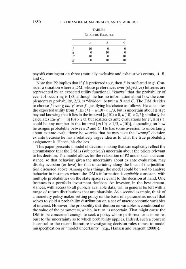
SAVAGE’S AXIOM P2, often referred to as the sure thing principle, states that,if two acts are equal on a given event, then it should not matter (for rank-ing the acts in terms of preferences) what they are equal to on that event. Ithas been observed, however, that there is at least one kind of circumstancewhere a decision maker (DM) might find the principle less persuasive—if theDM were worried by cognitive or informational constraints that leave him un-certain about what odds apply to the payoff relevant events. Ellsberg (1961)presented examples inspired by this observation; Table I is a stylized descrip-tion of one of those examples. The table shows four acts, fg f ′, and g′, with
1We thank N. Al-Najjar, E. Dekel, D. Fudenberg, S. Grant, Y. Halevy, I. Jewitt, B. Lipman,F. Maccheroni, S. Morris, R. Nau, K. Nehring, W. Neilson, K. Roberts, U. Segal, A. Shneyerov,J.-M. Tallon, R. Vohra, P. Wakker, and especially L. Epstein, I. Gilboa, M. Machina, andT. Strzalecki for helpful discussions and suggestions. We also thank three referees and the co-editor for offering very useful comments and advice. We also thank a number of seminar andconference audiences. We thank MEDS at Northwestern University, ICER at the University ofTorino, and Eurequa at the University of Paris 1 for their hospitality during visits when part ofthe research was completed. Mukerji gratefully acknowledges financial support from the ESRCResearch Fellowship Award award R000 27 1065 and Marinacci gratefully acknowledges the fi-nancial support of MIUR. Tomasz Strzalecki provided excellent research assistance.
1849
1850 P. KLIBANOFF, M. MARINACCI, AND S. MUKERJI
TABLE I
ELLSBERG EXAMPLE
A B C
f 10 0 0g 0 10 0f ′ 10 0 10g′ 0 10 10
payoffs contingent on three (mutually exclusive and exhaustive) events, A, B,and C .
Note that P2 implies that if f is preferred to g, then f ′ is preferred to g′. Con-sider a situation where a DM, whose preferences over (objective) lotteries arerepresented by an expected utility functional, “knows” that the probability ofevent A occurring is 1/3, although he has no information about how the com-plementary probability, 2/3, is “divided” between B and C . The DM decidesto choose f over g but g′ over f ′, justifying his choice as follows. He calculatesthe expected utility from f , Eu(f )= u(10)× 1/3, but is uncertain about Eu(g)beyond knowing that it lies in the interval [u(10)×0u(10)×2/3]; similarly, hecalculates Eu(g′)= u(10)×2/3, but realizes ex ante evaluations for f ′, Eu(f ′),could be any number in the interval [u(10)× 1/3u(10)], depending on howhe assigns probability between B and C . He has some aversion to uncertaintyabout ex ante evaluations: he worries that he may take the “wrong” decisionex ante because he has a relatively vague idea as to what the true probabilityassignment is. Hence, his choices.
This paper presents a model of decision making that can explicitly reflect thecircumstance that the DM is (subjectively) uncertain about the priors relevantto his decision. The model allows for the relaxation of P2 under such a circum-stance, so that behavior, given the uncertainty about ex ante evaluation, maydisplay aversion (or love) for that uncertainty along the lines of the justifica-tion discussed above. Among other things, the model could be used to analyzebehavior in instances where the DM’s information is explicitly consistent withmultiple probabilities on the state space relevant to the decision at hand. Oneinstance is a portfolio investment decision. An investor, in the best circum-stances, with access to all publicly available data, will in general be left with arange of return distributions that are plausible. As a second example, think ofa monetary policy maker setting policy on the basis of a parametric model thatsolves to yield a probability distribution on a set of macroeconomic variablesof interest. However, the probability distribution on variables is conditional onthe value of the parameters, which, in turn, is uncertain. That might cause theDM to be concerned enough to seek a policy whose performance is more ro-bust to the uncertainty as to which probability applies. Indeed, such a concernis central to the recent literature investigating decision rules robust to modelmisspecification or “model uncertainty” (e.g., Hansen and Sargent (2000)).
DECISION MAKING UNDER AMBIGUITY 1851
Preferences characterized in this paper are shown to be represented by afunctional of the double expectational form,
V (f )=∫∆
φ
(∫S
u(f )dπ
)dµ≡ Eµφ(Eπu f )(1)
where f is a real-valued function defined on a state space S (an “act”), u is avon Neumann–Morgenstern (vN–M) utility function, π is a probability mea-sure on S, and φ is a map from reals to reals. There may be subjective uncer-tainty about what the “right” probability on S is: µ is the DM’s subjective priorover ∆, the set of possible probabilities π over S, and therefore measures thesubjective relevance of a particular π as the “right” probability. While u, asusual, characterizes attitude toward pure risk, we show that ambiguity attitudeis captured by φ. In particular, a concave φ characterizes ambiguity aversion,which we define to be an aversion to mean preserving spreads in µf , whereµf is the distribution over expected utility values induced by µ and f . Thedistribution µf represents the uncertainty about ex ante evaluation; it showsthe probabilities of different evaluations of the act f We define behaviorallywhat it means for a DM’s belief about an event to be ambiguous and go on toshow that, in our model, this definition is essentially equivalent to the DM be-ing uncertain about the probability of the event, thereby identifying ambiguitywith uncertainty/multiplicity with respect to relevant priors and, hence, ex anteevaluations. It is worth noting that this preference model does not, in general,impose reduction between µ and the π’s in the support of µ. Such reductionoccurs only when φ is linear, a situation that we show is identified with ambi-guity neutrality and wherein the preferences are observationally equivalent tothose of a subjective expected utility maximizer. The idea of modeling ambigu-ity attitude by relaxing reduction between first and second order probabilitiesfirst appeared in Segal (1987) and inspires the analysis in this paper.
The basic structure of the model and assumptions are as follows. Our focusof interest is the DM’s preferences over acts on the state space S. This set ofacts is assumed to include a special subset of acts that we call lotteries, i.e.,acts measurable with respect to a partition of S over which probabilities areassumed to be objectively given (or unanimously agreed upon). We start by as-suming preferences over these lotteries are expected utility preferences. Frompreferences over lotteries, the DM’s risk preferences are revealed, representedby vN–M index u. We then consider preferences over acts each of whose payoffis contingent on which prior (on S) is the “right” probability: we call these actssecond order acts. For the moment, to fix ideas, think of these acts as “betsover the right prior.” Our second assumption states that preferences over sec-ond order acts are subjective expected utility (SEU) preferences. The point ofdefining second order acts and imposing Assumption 2 is to model explicitlythe uncertainty about the “right probability” and uncover the DM’s subjectivebeliefs with respect to this uncertainty and attitude to this uncertainty. Indeed,
1852 P. KLIBANOFF, M. MARINACCI, AND S. MUKERJI
following this assumption, we recover µ and v: the former is a probability mea-sure over possible priors on S that reveal the DM’s beliefs, whereas the latteris the vN–M index that summarizes the DM’s attitude toward the uncertaintyover the “right” prior. Our third assumption connects preferences over secondorder acts to preferences over acts on S. The assumption identifies an act f ,defined on S, with a second order act that yields, for each prior π on S, the cer-tainty equivalent of the lottery induced by f and π. Upon setting φ≡ v u−1,the three assumptions lead to the representation given in (1).
Intuitively, ambiguity averse DMs prefer acts whose evaluation is more ro-bust to the possible variation in probabilities. In our model that is translated asan aversion to mean preserving spreads in the induced distribution of expectedutilities, µf . This is shown to be equivalent to concavity of φ and to the DMbeing more averse to the subjective uncertainty about priors than he is to therisk in lotteries. In an investment problem, we may think of second order actsas bets on which return distribution is right. It is as if we imagine an ambiguityaverse DM to be thinking as follows: “My best guess of the chance that thereturn distribution is ‘π’ is 20%. However, this is based on ‘softer’ informationthan knowing that the chance of a particular outcome in an objective lotteryis 20%. Hence, I would like to behave with more caution with respect to theformer risk.”
Apart from providing (what we think is) a clarifying perspective on ambi-guity and ambiguity attitude, this functional representation will be particularlyuseful in economic modeling to answer comparative statics questions that in-volve ambiguity. Take an economic model where agents’ beliefs reflect someambiguity. Next, without perturbing the information structure, suppose wewanted to ask how the equilibrium would change if the extent of ambiguityaversion were to decrease; e.g., if we were to replace ambiguity aversion withambiguity neutrality, holding information and risk attitude fixed. Another use-ful comparative statics exercise is to hold ambiguity attitudes fixed and askhow the equilibrium is affected if the perceived ambiguity is varied. Workingout such comparative statics properly requires a model that allows a concep-tual/parametric separation of (possibly) ambiguous beliefs and ambiguity atti-tude, analogous to the distinction usually made between risk and risk attitude.The model and functional representation in the paper allow this separation,whereas such a separation is not evident in the pioneering and most popu-lar decision making models that incorporate ambiguity, namely, the maxminexpected utility (MEU) preferences (Gilboa and Schmeidler (1989)) and theChoquet expected utility model of Schmeidler (1989). A more recent contri-bution, Ghirardato, Maccheroni, and Marinacci (2004), axiomatizes a modeltermed α-MEU wherein it is possible in a certain sense to differentiate am-biguity attitude from ambiguity. A more detailed discussion of this model isdeferred until Section 5.1. As will be explained in that discussion, the α-MEUmodel does not, in general, facilitate the first comparative static exercise men-tioned above.
DECISION MAKING UNDER AMBIGUITY 1853
To illustrate how our model can facilitate comparative statics, we include, inthe final section of the paper, an (numerical) analysis of two simple portfoliochoice problems. The analysis considers how the choice of an optimal portfoliois affected when ambiguity attitude is varied. This allows a comparison of theeffects of risk attitude in expected utility with that of ambiguity attitude.
The rest of the paper is organized as follows. Section 2 states our main as-sumptions and derives the representation. Section 3 defines ambiguity attitudeand characterizes it in terms of the representation. Section 4 gives a behavioraldefinition of an ambiguous event and relates this definition to the representa-tion. Section 5 discusses related literature. Finally, Section 6 presents the sim-ple portfolio choice problems. There is a brief concluding section. All proofs,unless otherwise noted in the text, appear in the Appendix.
2. ASSUMPTIONS AND REPRESENTATION
2.1. Preliminaries
Let A be the Borel σ-algebra of a separable metric space Ω and let B1 bethe Borel σ-algebra of (01]. Consider the state space S =Ω× (01], endowedwith the product σ-algebra Σ ≡ A ⊗ B1. For the remainder of this paper, allevents will be assumed to belong to Σ unless stated otherwise.
We denote by f :S → C a Savage act, where C is the set of consequences.We assume C to be an interval in R that contains the interval [−11]. Givena preference on the set of Savage acts, F denotes the set of all boundedΣ-measurable Savage acts; i.e., f ∈ F if s ∈ S : f (s) x ∈ Σ for each x ∈ Cand if there exist x′x′′ ∈ C such that x′ f x′′.
The space (01] is introduced simply to model a rich set of lotteries as a set ofSavage acts. An act l ∈F is said to be a lottery if l depends only on (01]—i.e.,l(ω1 r) = l(ω2 r) for any ω1ω2 ∈ Ω and r ∈ (01]—and it is Riemann inte-grable. The set of all such lotteries is L. If f ∈ L and r ∈ (01], we sometimeswrite f (r), meaning f (ω r) for any ω ∈Ω.2
Given the Lebesgue measure λ :B1 → [01], let π :Σ→ [01] be a count-ably additive product probability such that π(A×B)= π(A× (01])λ(B) forA ∈A and B ∈ B1. The set of all such probabilities π is denoted by ∆. LetC(S) be the set of all continuous (with respect to (w.r.t.) the product topologyof S) and bounded real-valued functions on S. Using C(S) we can equip ∆ with
2Our modeling of lotteries in this way and use of a product state space is similar to the “single-stage” approach in Sarin and Wakker (1992, 1997) and to Anscombe–Aumann-style models. Bythe phrase “a rich set of lotteries,” we simply mean that, for any probability p ∈ [01], we mayconstruct an act that yields a consequence with that probability. While this richness is not requiredin the statement of our axioms or in our representation result, it is invoked later in the paper inTheorems 2 and 3.
1854 P. KLIBANOFF, M. MARINACCI, AND S. MUKERJI
the vague topology, that is, the coarsest topology on ∆ that makes the followingfunctionals continuous:
π →∫ψdπ for each ψ ∈C(S) and π ∈ ∆
Throughout the paper we assume ∆ to be endowed with the vague topol-ogy. Let σ(∆) be the Borel σ-algebra on ∆ generated by the vague topology.Lemma 5 in the Appendix shows a property of σ(∆) that we use to guaranteethat the integrals in our main representation theorem are well defined.
Since we wish to allow ∆ to be another domain of uncertainty for the DMapart from S, we model it explicitly as such. Does the DM regard this domainas uncertain and if so, what are the DM’s beliefs? To formally identify this,we look at preferences over second order acts, which assign consequences toelements of ∆.
DEFINITION 1: A second order act is any bounded σ(∆)-measurable functionf :∆→ C that associates an element of ∆ to a consequence. We denote by F theset of all second order acts.
Let 2 be the DM’s preference ordering over F. The main focus of the modelis , a preference relation defined on F (the set of acts on S) It might behelpful at this point to relate our structure to a more standard Savage-likeone. Consider a product state space S × ∆ In a Savage-type theory with thisstate space, the objects of choice—Savage acts—would be all (appropriatelymeasurable) functions from S × ∆ to an outcome space C. The theory wouldthen take as primitive preferences over Savage acts. In contrast, our theoryconcerns preferences over only two subsets of Savage acts—those acts thatdepend either only on S or only on ∆We do not consider any acts that dependon both nor do we explicitly consider preferences between these two subsets.
While, formally, our second order acts may be considered to be a subsetof Savage acts, there is a question whether preferences with respect to theseacts are observable. The mapping from observable events to events in ∆ maynot always be evident. When it is not evident we may need something richerthan behavioral data, perhaps cognitive data or thought experiments, to helpus reveal the DM’s beliefs over ∆.
However, we would like to suggest that second order acts are not as strangeor unfamiliar as they might first appear. Consider any parametric setting, i.e.,a finite dimensional parameter space Θ, such that ∆ = πθθ∈Θ. Second orderacts would simply be bets on the value of the parameter. In a parametric port-folio investment example, these could be bets about the parameter values thatcharacterize the asset returns, e.g., means, variances, and covariances. Simi-larly, in model uncertainty applications, second order acts are bets about thevalues of the relevant parameters in the underlying model. Closer to decisiontheory, for an Ellsberg urn, second order acts may be viewed as bets on thecomposition of the urn.
DECISION MAKING UNDER AMBIGUITY 1855
2.2. Main Assumptions
Next we describe three assumptions on the preference orderings and 2.The first assumption applies to the preference ordering when restricted tothe domain of lottery acts. Preferences over the lotteries are assumed to havean expected utility representation.
ASSUMPTION 1 —Expected Utility on Lotteries: There exists a unique u :C→ R continuous, strictly increasing, and normalized so that u(0) = 0 andu(1) = 1 such that, for all fg ∈ L, f g if and only if
∫(01] u(f (r))dr ≥∫
(01] u(g(r))dr
In the standard way, the utility function, u, represents the DM’s attitudetoward risk generated from the lottery part of the state space. 3 The next as-sumption is on 2, the preferences over second order acts. These preferencesare assumed to have a subjective expected utility representation.
ASSUMPTION 2—Subjective Expected Utility on Second Order Acts: Thereexists a countably additive probability µ :σ(∆)→ [01] with some J ∈ σ(∆) suchthat 0 < µ(J) < 1 and a continuous, strictly increasing v :C → R, such that, forall fg ∈ F,
f 2 g ⇐⇒∫∆
v(f(π))dµ≥∫∆
v(g(π))dµ
Moreover, µ is unique and v is unique up to positive affine transformations.
We denote by Π the support of µ, that is, the smallest closed (w.r.t. thevague topology) subset of ∆ whose complement has measure zero; Π is thesubset of ∆ that the DM subjectively considers relevant. Given any E ⊆Π, weinterpret µ(E) as the DM’s subjective assessment of the likelihood that therelevant probability lies in E; hence, µ may be thought of as a “second orderprobability” over the first order probabilities π.4 Notice that Π may well be afinite subset of ∆. Finally, the utility function v represents the DM’s attitudetoward risk generated by payoffs contingent on events in ∆.
3An alternative approach to deriving risk attitude, suggested to us by Mark Machina, would beto assume appropriate smoothness of our preferences and apply Machina (2004) to identify riskattitudes with preferences over “almost-objective” acts. It may be verified, given our representa-tion, that such preferences are entirely determined by u(·)
4We assume that µ is countably additive to avoid going into technicalities that involve the sup-port. In any case, this is likely to be assumed in any application and, as a matter of theory, Arrow(1971) showed that countably additive probabilities can be derived in an SEU model by addinga monotone continuity axiom. As Arrow (1971, p. 48) remarked, “the assumption of MonotoneContinuity seems, I believe correctly, to be the harmless simplification almost inevitable in theformalization of any real-life problem.” Furthermore, the foundations for Assumption 2 that wecite in the next paragraph also show how to deliver countable additivity.
1856 P. KLIBANOFF, M. MARINACCI, AND S. MUKERJI
Each of the first two assumptions could be replaced by more primitive as-sumptions on and 2, respectively, that deliver the expected utility rep-resentations. For example, Assumption 1 can be derived along the lines ofGrandmont (1972) by identifying lottery acts with their respective distribu-tions. Theorem V.6.1 of Wakker (1989) applied to 2 over second order actscan be used to deliver Assumption 2. This theorem is an axiomatic characteri-zation of continuous subjective expected utility for acts that map from generalstate spaces to suitably rich consequence spaces. The key axiom in Wakker’streatment is a condition that requires consistency of trade-offs revealed bypreferences. These or any other axioms applied to second order acts may notalways be easily verifiable, because the payoffs of these acts are contingent onelements of ∆ As observed earlier, in some instances it may not be possibleto empirically verify which element in ∆ actually obtains. On the other hand,such empirical verification may be relatively simple in experimental settings: inEllsberg urn experiments, all you would need to do is dump the urn and verifythe proportion of balls in it. Verification may also be possible if one has theopportunity to wait and observe a sufficiently long run of data generated byrepeated realizations from the π ∈ ∆ that obtains. For instance, a finance pro-fessional using a parametric model to evaluate portfolios, where parametersdetermine the relevant stochastic process on returns, may obtain (economet-ric) estimates of the true parameter value if there is enough stationarity in thedata generating process.
Even when verifiability is an issue, preference axioms provide a useful con-ceptual underpinning to choice criteria. For example, economists often applythe subjective expected utility model to a variety of situations characterized bylimited verifiability. For instance, consider an investor’s portfolio choice prob-lem. The relevant states of the world for a particular stock may include eventsthat take place inside the firm and in the wider market. It cannot be claimedthat it is easy to verify, if at all, which of these relevant states actually obtain.Similarly, subjective expected utility is used to model agents in situations ofasymmetric information, in a Bayesian game for example, where agents havebeliefs about private signals and even beliefs about other players’ beliefs. Be-cause signals and beliefs are private, it may not be possible for an observer toverify which of them actually are realized. Nevertheless, in such situations pref-erence axioms are commonly invoked to justify the use of the expected utilitycriterion and play a useful role in understanding the meaning of this criterion.In much the same way, we believe axioms on second order acts provide a sen-sible foundation for our assumption of subjective expected utility over secondorder acts. It is an open question whether an identical representation could bederived using only preferences over acts in F .
Our final main assumption requires the preference ordering of primary in-terest, , to be consistent with Assumptions 1 and 2 in a certain way. Beforestating the assumption, we require a few preliminaries. An act f and a prob-ability π induce a probability distribution πf on consequences. To define this
DECISION MAKING UNDER AMBIGUITY 1857
formally, denote by Bc the Borel σ-algebra of C and define πf :Bc → [01] byπf(B) = π(f−1(B)) for all B ∈ Bc . The next lemma shows that each distribu-tion πf can be “replicated” by a suitable lottery act.
LEMMA 1: Given any f ∈ F and any π ∈ ∆, there exists a (nondecreasing)lottery act lf (π) ∈L that has the same distribution as πf , i.e., such that λ(lf (π) ∈B)= πf(B) for all B ∈ Bc .
NOTATION 1: In what follows, δx denotes the constant act with consequencex ∈ C and cf (π) denotes the certainty equivalent of the lottery act lf (π); i.e.,δcf (π) ∼ lf (π)
Notice that since u is continuous and strictly increasing (Assumption 1), lot-tery acts have a unique certainty equivalent.
Since f together with a possible probability π generates a distribution overconsequences identical to those generated by lf (π), we assume (for consistencywith Assumption 1) that the certainty equivalent of f , given π, is the same asthe certainty equivalent of lf (π). Thus, as the certainty equivalent of f dependson which π is the right probability law, facing f is like facing a second order act,f 2, yielding cf (π) for each particularπ This motivates the following definition.
DEFINITION 2: Given f ∈ F , f 2 ∈ F denotes a second order act associatedwith f defined as
f 2(π)= cf (π) for all π ∈ ∆The assumption below says that the DM agrees with the reasoning above
and therefore orders acts f ∈F identically to the associated second order actsf 2 ∈ F
ASSUMPTION 3—Consistency with Preferences over Associated Second Or-der Acts: Given fg ∈F and f 2 g2 ∈ F,
f g ⇐⇒ f 2 2 g2
2.3. The Representation
The preceding three assumptions are basic to our model in that they areall that we invoke to obtain our representation result. Theorem 1 shows thatgiven these assumptions, is represented by a functional that is an “expectedutility over expected utilities.” Evaluation of f ∈F proceeds in two stages: first,compute all possible expected utilities of f , each expected utility correspondingto a π in the support of µ; next, compute the expectation (with respect to themeasure µ) of the expected utilities obtained in the first stage, each expectedutility transformed by the increasing function φ.
1858 P. KLIBANOFF, M. MARINACCI, AND S. MUKERJI
As will be shown in subsequent analysis, this representation allows a decom-position of the DM’s tastes and beliefs: u determines risk attitude toward acts,φ determines ambiguity attitude in the sense that a concave (convex)φ impliesambiguity aversion (ambiguity loving), and µ determines the subjective belief,including any ambiguity perceived therein by the DM.
NOTATION 2: Let U denote the range u(x) :x ∈ C of the utility function u
THEOREM 1: Given Assumptions 1, 2, and 3, there exists a continuous andstrictly increasing φ :U → R such that is represented by the preference func-tional V :F → R given by
V (f )=∫∆
φ
[∫S
u(f (s))dπ
]dµ≡ Eµφ(Eπu f )(2)
Given u, the function φ is unique up to positive affine transformations. Moreover,if u= αu+β, α> 0, then the associated φ is such that φ(αy+β)=φ(y), wherey ∈ U .
PROOF: By Assumption 3, f g⇔ f 2 2 g2. By Assumption 2, f 2 2 g2 ⇔∫v(cf (π))dµ≥ ∫
v(cg(π))dµ Hence,
f g ⇐⇒∫v(cf (π))dµ≥
∫v(cg(π))dµ(3)
Since v and u are strictly increasing, v(cf (π))=φ(u(cf (π))) for some strictlyincreasing φ. Since v and u are continuous, so is φ. Substituting for v(cf (π))in (3), we get
f g ⇐⇒∫φ
(u(cf (π))
)dµ≥
∫φ
(u(cg(π))
)dµ(4)
Now, recall,
δcf (π) ∼ lf (π) ⇐⇒ u(cf (π))=∫(01]
u(lf (π)(r))dr
So,
u(cf (π))=∑
x∈supp(πf )
u(x)πf (x)=∫S
u(f (s))dπ(5)
Thus, substituting (5) into (4),
f g ⇐⇒∫φ
(∫S
u(f (s))dπ
)dµ≥
∫φ
(∫S
u(g(s))dπ
)dµ
DECISION MAKING UNDER AMBIGUITY 1859
This proves the representation claim in the theorem. To see the uniquenessproperties of φ, notice that
v(cf (π))=φ(u(cf (π))
) ⇐⇒ φ(y)= v(u−1(y))
Let u= αu+β and let y ∈ U Then
(u−1)(αy +β)= x : u(x)= αy +β= x :αu(x)+β= αy +β= x :u(x)= y= u−1(y)
Hence, ∀ y ∈ U , φ(αy +β)= (v u−1)(αy +β)= (v u−1)(y)=φ(y). Finally,v is unique up to positive affine transformations according to Assumption 2,so, fixing u, φ is as well. Q.E.D.
The integrals in (2) are well defined because of Lemma 5 in the Appendix,which guarantees their existence. Hereafter, when we write a preference rela-tion , we assume that it satisfies the conditions in Theorem 1. This theoremcan be viewed as a part of a more comprehensive representation result (re-ported in Section A.2 as Theorem 4) for the two orderings and 2 in whichAssumptions 1, 2, and 3 are both necessary and sufficient. Theorem 4 also notesexplicitly an important point evident in the proof of Theorem 1, that φ equalsv u−1. The functional representation is also invariant to positive affine trans-forms of the vN–M utility index that applies to the lotteries. That is, when u istranslated by a positive affine transformation to u′, the class of associated φ′ issimply the class of φ with domain shifted by the positive affine transformation.
We close this subsection by observing that, though Assumption 1 imposedexpected utility preferences on lotteries, we could relax that assumption byallowing the preferences over lotteries to be rank dependent expected util-ity preferences (see Quiggin (1993)) with a suitable probability distortionϕ : [01] → [01]. Then the representation of preferences over acts in F is asgiven in the following corollary.
COROLLARY 1: Suppose there exists a continuous and nondecreasing functionϕ : [01] → [01] such that, for all fg ∈ L, f g if and only if
∫(01] u(f (r))×
dϕ(λ)≥ ∫(01] u(g(r))dϕ(λ). If satisfies Assumptions 2 and 3, then (2) of The-
orem 1 becomes
V (f )=∫∆
φ
[∫S
u(f (s))dϕ(π)
]dµ(6)
PROOF: It is enough to observe that here (5) becomes u(cf (π)) =∫Su(f (s))dϕ(π).
1860 P. KLIBANOFF, M. MARINACCI, AND S. MUKERJI
The rest of the proof is identical to that of Theorem 1. Q.E.D.
Note that while the outer integral is the usual one, the inner integral in (6) isa Choquet integral, and the inner and outer integrals are well defined becauseof Lemma 5.
3. AMBIGUITY ATTITUDE
In this section we first provide a definition of a DM’s ambiguity attitude andshow that this ambiguity attitude is characterized by properties ofφ, one of thefunctions from our representation above. Comparison of ambiguity attitudesacross preference relations is dealt with in Section 3.2. Finally, Section 3.3 de-scribes a useful regularity condition on ambiguity attitudes. It also shows thatthis condition is implied by our other assumptions if φ is twice continuouslydifferentiable.
3.1. Characterizing Ambiguity Attitude
To discuss ambiguity attitude, we first require an additional assumption. Inthe classical theory, it is commonly implicitly or explicitly assumed or derivedthat a given individual will display the same risk attitude across settings inwhich she might hold different subjective beliefs. We would like to assumethe same. In the context of our theory, this entails the assumption that riskattitudes derived from lotteries and risk attitudes derived from second orderacts are independent of an individual’s beliefs. In fact, a weaker assumptionsuffices for our purposes: the assumption that the two risk attitudes u and v donot vary with Π, the support of an individual’s belief µ.
To state this formally in our setting, consider a family Π2ΠΠ⊆∆ of pairs
of preference relations (over acts and over second order acts, respectively) thatcharacterize each DM. There is a pair of preference relations that correspondto each possible support Π, that is, to each possible state of information theDM may have about which probabilities π (over S) are relevant to his de-cision problem. Assumptions 4 and 5, which follow here and in Section 3.3,require certain properties of preferences to hold across the different pairsΠ2
ΠΠ⊆∆. We emphasize that these assumptions are of a somewhat differ-ent nature than the three assumptions of the previous section. While the earlierassumptions operate only within pairs of preferences (Π2
Π), Assumptions4 and 5 operate across the entire family of pairs of preferences.
For all the definitions, assumptions, and results to come, it would be enoughif everywhere that we state something about an entire family Π2
ΠΠ⊆∆ ofpairs of preference relations, we limit our statement to the pair of original pref-erences (2) and a pair Π2
Π withΠ that contains exactly two measures
DECISION MAKING UNDER AMBIGUITY 1861
that have disjoint support.5 While we stick with the stronger formulations thatuse all Π for ease of statement, this observation indicates that many fewerpairs of preference relations need to be considered (two rather than an infinitenumber) than the stronger versions would lead one to think.
ASSUMPTION 4—Separation of Tastes and Beliefs: Fix a family of preferencerelationships Π2
ΠΠ⊆∆ for a given DM.(i) The restriction of Π to lottery acts remains the same for every support
Π ⊆ ∆.(ii) The same invariance with respect toΠ holds for the risk preferences derived
from 2Π
Imposing Assumption 4 in addition to the earlier assumptions guaranteesthat as the support of a DM’s subjective belief varies (say, due to conditioningon different information), the DM’s attitude toward risk in lotteries, as em-bodied in u (from Assumption 1), and attitude toward risk on the space ∆, asembodied in v (from Assumption 2), remain unchanged. Importantly, this willalso mean that the same φmay be used to represent each Π for a DM. To seethis, recall that φ is v u−1.
Notice that there is no restriction on the DM’s belief associated with each Π
and 2Π except that of having support Π. Although we do not need to assume
it for our results, a natural possibility is that all such beliefs are connected viaconditioning from some “original” common belief.
We now proceed to develop a formal notion of ambiguity attitude. Recallthat an act f together with a probability π induces a distribution πf on conse-quences. Each such distribution is naturally associated with a lottery lf (π) ∈L,which has a certainty equivalent cf (π). Fixing an act f , the probability µ maythen be used to induce a measure µf on u(cf (π)) :π ∈Π, the set of expectedutility values generated by f corresponding to the different π’s inΠ (using theutility function u from Assumption 1). When necessary, we denote the beliefassociated with Π by µΠ and the corresponding µf by µΠf To introduce µfformally, we need the following lemma. Here Bu denotes the Borel σ-algebraof U and u(B)= u(x) :x ∈ B.6
LEMMA 2: We have Bu = u(B) :B ∈ Bc.
5The significance of two measures with disjoint support is that they allow the entire spaceof pairs of expected utility values to be generated by varying the act under consideration. Thisrichness is needed for preference over acts to fully pin down convexity properties of φ. Suchrichness comes for free in expected utility theory because acts are not summed over states beforethe utility function is applied.
6Since U is an interval, Bu coincides with the restriction on U of the Borel σ-algebra B ofthe real line. The same applies to B1 and Bc , which are the restrictions of B on (01] and C,respectively.
1862 P. KLIBANOFF, M. MARINACCI, AND S. MUKERJI
By Lemma 2, µf is defined on Bu.
DEFINITION 3: Given f ∈ F , the induced distribution µf :Bu → [01] isgiven by
µf(u(B))≡ µ((f 2)−1(B)
)for each B ∈ Bc
Given an act f , the derived (subjective) probability distribution over ex-pected utilities, µf , smoothly aggregates the information the DM has aboutthe relevant π’s and how each such π evaluates f without imposing reductionbetween µ and the π’s. In this framework the induced distribution µf repre-sents the DM’s subjective uncertainty about the “right” (ex ante) evaluationof an act. The greater the spread in µf , the greater the uncertainty about theex ante evaluation. In our model it is this uncertainty through which ambigu-ity about beliefs may affect behavior: ambiguity aversion is an aversion to thesubjective uncertainty about ex ante evaluations. Analogous to risk aversion,aversion to this uncertainty is taken to be the same as disliking a mean preserv-ing spread in µf .7 Just as in the theory of risk aversion, this may be expressedas a preference for getting a sure “average” to getting the act that induces µf .To state this formally, we need notation for the mean of µf , i.e., for the averageexpected utility from f
NOTATION 3: Let e(µf )≡ ∫U xdµf . Notice u−1(e(µf )) ∈ C
Thus δu−1(e(µf ))is the constant act valued at the average utility of f .
DEFINITION 4: A DM displays smooth ambiguity aversion at (fΠ) if
δu−1(e(µf ))Π f
where µ has support Π A DM displays smooth ambiguity aversion if she dis-plays smooth ambiguity aversion at (fΠ) for all f ∈F and all supportsΠ ⊆ ∆.
In a similar way, we can define smooth ambiguity love and neutrality. Theproposition below shows that smooth ambiguity aversion is characterized inthe representing functional by the concavity of φ. The proposition also showsthat smooth ambiguity aversion is equivalent to the DM being more risk averseto the subjective uncertainty about the right prior on S than he is to the riskgenerated by lotteries (whose probabilities are objectively known). A resultcharacterizing smooth ambiguity love by convexity of φ follows from the sameargument. Similarly, smooth ambiguity neutrality is characterized by φ linear.
7It is important to keep in mind the distinction between µ and µf : while µ is a measure onprobabilities and does not vary with f , µf is a measure on utilities and depends on f .
DECISION MAKING UNDER AMBIGUITY 1863
It is worth noting that a straightforward adaptation of the proof of the analo-gous result in risk theory does not suffice here. The reason is that the neededdiversity of associated second order acts is not guaranteed in general.
PROPOSITION 1: Under Assumptions 1–4, the following conditions are equiva-lent:
(i) The function φ :U → R is concave.(ii) Attitude v is a concave transform of u.(iii) The DM displays smooth ambiguity aversion.
The proposition has the following corollary (whose simple proof is omitted),which shows that the usual reduction (between µ and π) applies wheneverambiguity neutrality holds. In that case, we are back to subjective expectedutility. An ambiguity neutral DM, though informed of the multiplicity of π’s, isindifferent to the spread in the ex ante evaluation of an act caused by this mul-tiplicity; the DM only cares about the evaluation using the “expected prior” η.
COROLLARY 2: Under Assumptions 1–4, the following properties are equiva-lent:
(i) The DM is smoothly ambiguity neutral.(ii) The function φ is linear.(iii) The preference functional V (f ) = ∫
Su(f (s))dη, where η(E) =∫
∆π(E)dµ for all E ∈ Σ.
REMARK 1: An ambiguity averse DM in this model prefers the lottery act,, that pays x with an objective probability p (and 0 with probability 1 −p) tothe second order act, f 2, that pays x contingent on an event E ⊆ ∆ to whichthe DM assigns a subjective prior µ(E)= p (and pays 0 elsewhere). These twooptions expose the DM to the same uncertainty over payoffs generated in twodifferent ways. Ambiguity aversion is the relative dislike of payoff uncertaintygenerated by subjective beliefs over probability distributions on S compared topayoff uncertainty generated by lotteries.
Notice that this model does not deal with objective probabilities on ∆; µ isa subjective measure. However, it may be useful to suggest one interpreta-tion of how an “objective µ” might be viewed by the DM. Suppose the DM isinformed that each π ∈ ∆ obtains with an objective probability p(π), gener-ated, for example, by a randomizing device, such as a roulette wheel. It seemsplausible that the DM would then view the second order act f 2 as equivalentto the lottery act The interpretation seems appropriate since f 2 and areidentified with identical objective probability distributions over consequences.More generally, in such a case second order acts can be regarded as lotteries,so there is no motivation to distinguish between v and u, i.e., v = u Hence
1864 P. KLIBANOFF, M. MARINACCI, AND S. MUKERJI
φ is the identity and the DM evaluates acts by expected utility. Needless tosay this is only an interpretation. Being strictly formal, lotteries and secondorder acts are different objects. Hence, it is possible that v could be more con-cave than u even with objective probabilities. For some recent experimentalevidence on this point, see Halevy (2004). These interpretations are limited tothe case where the uncertainty about second order acts is wholly objective; it isfar from obvious what an appropriate interpretation is if this uncertainty werea combination of objective and subjective.
3.2. Comparison of Ambiguity Attitudes
In this section we study differences in ambiguity aversion across DMs. As inthe previous section, we identify each DM with a family of preferences Π2ΠΠ⊆∆, parametrized byΠ. Throughout the section, we assume Assumption 4
holds in addition to the first three assumptions. Hence, ambiguity attitudes donot depend on the support Π of µ.
We begin with our definition of what makes one preference order more am-biguity averse than another.
DEFINITION 5: Let A and B be two DMs whose families of preferencesshare the same probability measures µΠ for each support Π. We say that A ismore ambiguity averse than B if
f AΠ l ⇒ f B
Π l(7)
for every f ∈F , every l ∈L, and every support Π ⊆ ∆.
The idea behind this definition is that if two DMs, A and B, share the samebeliefs but B prefers an uncertain act over a (purely) risky act wheneverA doesso, then this must be due to B’s comparatively lower aversion to ambiguity.Given a lottery l, the set of uncertain acts that B prefers to l is larger thanA’s preferred set of uncertain acts. Since A and B share the same beliefs, theonly factor that could explain the larger set preferred by B is difference inattitudes to the uncertainty. However, differing attitudes toward lotteries (i.e.,risk) cannot be the reason. Given that the act f in preference condition (7) mayitself be a lottery act and that the condition holds for every l ∈L, it essentiallyfollows thatA and Bmust rank lotteries the same way, hence leaving ambiguityattitude as the only factor that may explain the difference in preferences.
We can now state our comparative result, which shows that differences inambiguity aversion across DMs who share the same belief µ are completelycharacterized by the relative concavity of their functions φ. Significantly, theresult shows that Definition 5 implies that ambiguity aversion is comparable
DECISION MAKING UNDER AMBIGUITY 1865
across two DMs only if their risk attitudes coincide.8 Note that the relative con-cavity of φ plays here a role analogous to the role of the relative concavity ofutility functions in standard risk theory.
THEOREM 2: LetA and B be two DMs whose families of preferences share thesame probability µΠ for each supportΠ. ThenA is more ambiguity averse than Bif and only if they share the same (normalized) vN–M utility function u and
φA = h φBfor some strictly increasing and concave h :φB(U)→ R.
Using results from standard risk theory, we get the following corollary as animmediate consequence of Theorem 2.
COROLLARY 3: Suppose the hypothesis of Theorem 2 holds. If φA and φB aretwice continuously differentiable, then A is more ambiguity averse than B if andonly if they share the same (normalized) vN–M utility function u and, for everyx ∈ U ,
−φ′′A(x)
φ′A(x)
≥ −φ′′B(x)
φ′B(x)
Analogous to risk theory, we will call the ratio
α(x)= −φ′′(x)φ′(x)
the coefficient of ambiguity aversion at x ∈ U .
COROLLARY 4: A DM’s preferences are represented using a concave φ if andonly if he is more ambiguity averse than some expected utility DM (i.e., a DM allof whose associated preferences Π are expected utility).
REMARK 2: Corollary 4 connects our definition of smooth ambiguity aver-sion (Definition 4) to the comparative notion of ambiguity aversion in Defi-nition 5. It shows that they agree, with expected utility taken as the dividingline between ambiguity aversion and ambiguity loving. It can also be shown(see Klibanoff, Marinacci, and Mukerji (2003)) that if our Assumption 5 (pre-sented in the next section) holds, nothing would change if we were to takeprobabilistic sophistication, rather than expected utility, as the benchmark.
8This feature, that comparison of ambiguity attitudes is restricted to DMs with the same riskattitude, is shared by the α-MEU type models. See, for instance, Proposition 6 in Ghirardato,Maccheroni, and Marinacci (2004). It is also present in the approaches to comparative ambiguityaversion developed in Epstein (1999) and Ghirardato and Marinacci (2002).
1866 P. KLIBANOFF, M. MARINACCI, AND S. MUKERJI
We close this section by considering the two important special cases of con-stant and extreme ambiguity attitudes. We begin by defining a notion of con-stant ambiguity attitude.
DEFINITION 6: We say that the DM displays constant ambiguity attitude if,for each support Π ⊆ ∆,
f Π g ⇐⇒ f ′ Π g′
whenever acts f , g, f ′, and g′ are such that, for some k ∈ R and for each s ∈ S,
u(f ′(s))= u(f (s))+ k(8)
u(g′(s))= u(g(s))+ kRecall that under Assumption 1 (or a Grandmont (1972) style axiomatiza-
tion thereof) u may be recovered from preferences on lotteries only up to nor-malization. However, this is enough for the definition to be meaningful, sinceany quadruple of acts satisfies the conditions in the definition with u if and onlyif it satisfies such conditions with any renormalization u= αu+β for any α> 0and β ∈ R (the particular values of k relating the acts may change, but this isimmaterial).
To see the spirit of the definition, notice that by bumping up utility (not theraw payoffs) in each state by a constant amount we achieve a uniform shift inthe induced distribution over ex ante evaluations, i.e.,
µf ′(z+ k)= µf(z) and µg′(z+ k)= µg(z)The intuition of constant ambiguity attitude is that the DM views the “ambi-guity content” in µf and its “translation” µf ′ to be the same, and so rankingthem the same through preferences reveals ambiguity attitude unchanged bythe shift in well being. Next we show that constant ambiguity attitudes are char-acterized by an exponentialφ. It is of some interest to note that the propositiondoes not assume that φ is differentiable.
PROPOSITION 2: The DM displays constant ambiguity attitude if and only ifeither φ(x) = x for all x ∈ U or there exists an α = 0 such that φ(x) = − 1
αe−αx
for all x ∈ U , up to positive affine transformations.
We now turn to extreme ambiguity attitudes. The next proposition showsthat when ambiguity aversion is taken to infinity our model essentially exhibitsa maxmin expected utility behavior à la Gilboa and Schmeidler (1989), whereΠ is the given set of measures.9
9Tomasz Strzalecki helped us improve this result from that in an earlier version and provideda key step in its proof. Observe that when C is bounded, then by the Dini theorem, condition (iii)can be weakened to limn αn(x)= +∞ for all x ∈ U .
DECISION MAKING UNDER AMBIGUITY 1867
NOTATION 4: Set ess infΠ Eπu(f )= supt ∈ R :µΠ(π : Eπu(f ) < t)= 0.PROPOSITION 3: Let An be any sequence of DMs such that:
(i) all An share the same measures µΠ ;(ii) for all n, An+1 is more ambiguity averse than An;(iii) limn(infx∈U αn(x))= +∞;(iv) each φAn is everywhere twice continuously differentiable.Given any f and g in F , if f An
Π g for all n sufficiently large, then
ess infΠ
Eπu(f )≥ ess infΠ
Eπu(g)
Moreover,
ess infΠ
Eπu(f ) > ess infΠ
Eπu(g)
implies that, for all n large enough, f AnΠ g.
To make the connection to MEU, observe that when Π is finite, theness infΠ Eπu(f ) = minπ∈Π Eπu(f ). This also holds under standard topologicalassumptions, as the next lemma shows.
LEMMA 3: If f is upper semicontinuous (i.e., all preference intervals f xare closed), then ess infΠ Eπu(f ) = infΠ Eπu(f ). If, in addition, Π is compactand f is continuous, then ess infΠ Eπu(f )= minπ∈Π Eπu(f ).
We have claimed that our representation of preferences over acts in F allowsa separation of beliefs and tastes. We now make explicit the sense in which thisis so. In the representation, subjective beliefs (or information) are capturedby µ, including the ambiguity in the beliefs, as the results and discussion inSection 4 explain. With respect to tastes, three conceptually distinct attitudesare present in our model: risk attitude on acts in F , risk attitude on secondorder acts in F, and ambiguity attitude on acts in F . To what extent are therepresentations of these attitudes separately embodied in uv, and φ, respec-tively? It is clear from Assumption 1 that u represents risk attitude on lotteries(a subset of acts in F). However, given our three main assumptions, certaintyequivalents of acts in F given a probability π over S are the same as those ofthe corresponding lotteries. In this sense, u also represents risk attitude for allacts in F and not simply lotteries. (See footnote 3 for an additional justificationthat u represents risk attitude toward acts in F ) Assumption 2 guarantees thatv represents risk attitude on second order acts in F. Proposition 1 shows thatφ represents absolute ambiguity attitude on acts in F ; i.e., the shape of φ com-pletely determines whether the DM is ambiguity averse, ambiguity loving, orambiguity neutral. Theorem 2 shows the sense in which φ represents compara-tive ambiguity attitude; the comparison of ambiguity attitudes of two DMs who
1868 P. KLIBANOFF, M. MARINACCI, AND S. MUKERJI
share the same information, µ, is completely determined by the comparativeconcavity of the respective φ’s; however, the ambiguity attitudes of two DMsare not comparable if they do not share the same risk attitude, as representedby u. To claim a complete separation of these three attitudes and beliefs, itwould have to be possible to meaningfully compare properties of preferenceswith representations involving (arbitrarily) different specifications of µφ u,and v However, our separation is not complete in this sense because of twolimitations, which are explained next.
First, it is clear that a three-way separation of taste “parameters” φ, v, and uis not possible, because they are related by the equation φ= v u−1 Neverthe-less, it is equally clear that any two of these three parameters φ, v, and u maybe specified independently when using the model. For example, any φ may becombined with any u (and then v will be φ u). We are primarily interested inbehavior toward acts in F ; hence, the fact that we are able to specify φ and u(which, unlike v, represent attitudes toward acts in F) independently is ar-guably “good enough.” For instance, much of the impact of the well-knownpreference model due to Epstein and Zin (1989) rests on the fact that they,unlike standard models, allow a separation of intertemporal substitution fromintratemporal risk aversion. However, just as here, there are three attitudinalaspects of preference in their model: willingness to intertemporally substitute,intratemporal risk aversion, and preference over the timing of the resolutionof risk. Moreover, only two aspects may be specified separately, and once thisis done, the third is constrained. Nonetheless, it is customarily accepted thatin their model there is an effective separation of the two attitudes of pri-mary interest—intertemporal substitution and intratemporal risk aversion—and that this separation is good enough for economic modeling where one isless often interested in the third attitude.
A second limitation arises due to the fact that even though we may specifyφ, u, and µ independently of each other, our results limit the extent to whichwe may infer ambiguity attitude on the basis of φ when comparing preferencesacross these specifications. Comparing preferences of two DMs, we can infer(using Proposition 1) whether each DM is ambiguity averse or ambiguity lovingor neutral purely by looking at the shape of the φ’s in the respective specifica-tions, irrespective of the u’s and µ’s involved. However, Theorem 2 allows usto rank the two DMs in terms of their comparative ambiguity aversion on thebasis of the relative concavity of φ only when the DMs share the same µ and,furthermore, shows that we can only compare ambiguity aversion across thetwo when they share the same risk attitude, u (although there is no restrictionon the shared µ and u). As noted earlier, our approach is not unique in havingthis last feature.
Separation of this kind, with the two limitations mentioned, is neverthelessa significant advance in terms of what it allows in economic modeling. In par-ticular, it allows a comparison of two DMs who share the same beliefs and riskattitude toward acts, but one of whom is sensitive to expected utility (thus is
DECISION MAKING UNDER AMBIGUITY 1869
ambiguity neutral) and the other is sensitive to ambiguity, say ambiguity averse.This comparative static is important because it is precisely what is needed toanswer a question such as, “What is the pure effect of introducing ambiguitysensitivity into a given economic situation?” This is a most basic question andyet this cannot even be posed, let alone answered, within the framework ofthe other models of decision making that incorporate ambiguity such as MEU,CEU, and α-MEU. (See Section 5.1 for further clarification of this point.)
3.3. A Regularity Assumption on Ambiguity Attitude
In this section, we state a restriction on the DM’s preferences that requiresambiguity attitude to be “well behaved.” This good behavior will be useful inthe next section when we discuss ambiguous events and acts. In words, the re-striction is that if a preference is not neutral to ambiguity, then there existsat least one interval over which we require that the DM display either strictambiguity aversion or strict ambiguity love, but not both. What is ruled out isthe possibility that the DM’s ambiguity attitude everywhere flits between am-biguity aversion and ambiguity love, continuously from one point to the next.Note that it is entirely permissible that there be several intervals, over someof which the DM is ambiguity averse, while over others he is ambiguity loving.The statement of the assumption is immediately followed by a proposition thatgives an equivalent characterization in terms of φ
ASSUMPTION 5 —Consistent Ambiguity Attitude over Some Interval: TheDM’s family of preferences satisfies at least one of the following three conditions:
(i) Smooth ambiguity neutrality holds everywhere.(ii) There exists an open interval J ⊆ U such that smooth ambiguity aversion
holds strictly at all (fΠ) for which supp(µΠf ) is a nonsingleton subset of J.(iii) There exists an open intervalK ⊆ U such that smooth ambiguity love holds
strictly when limited to all (fΠ) for which supp(µΠf ) is a nonsingleton subsetof K.
PROPOSITION 4: Under Assumptions 1–4, we have the following:1. Assumption 5(i) holds if and only if φ linear.2. Assumption 5(ii) holds if and only ifφ strictly concave on some open interval
J ⊆ U .3. Assumption 5(iii) holds if and only if φ strictly convex on some open interval
K ⊆ U .
The following lemma and remark show that if φ were twice continuouslydifferentiable, as it is likely to be in any application, then Assumption 5 wouldactually be implied by the other assumptions and is not an additional assump-tion.
1870 P. KLIBANOFF, M. MARINACCI, AND S. MUKERJI
LEMMA 4: Suppose φ is twice continuously differentiable. If φ is not linear,then φ is either strictly concave or convex over some open interval.
REMARK 3: It follows immediately from Proposition 4 and Lemma 4 thatunder twice continuous differentiability of φ, Assumptions 1–4 imply Assump-tion 5. Note that the conclusion of Lemma 4 may not hold if the hypothesis isweakened to simply φ continuous.
4. AMBIGUITY
We have mentioned that an attractive feature of our model is that it allowsone to separate ambiguity from ambiguity attitude. In this section we concen-trate on the ambiguity part. First, we propose a preference based definition ofambiguity. We then show that this notion of ambiguity has a particularly simplecharacterization in our model. Finally, we briefly comment on the relationshipwith other notions of ambiguity.
What makes an event ambiguous or unambiguous by our definition rests ona test of behavior, with respect to bets on the event, inspired by the Ellsbergtwo-color experiment (Ellsberg (1961)). The role corresponding to bets on thedraw from the urn with the known mixture of balls is played here by bets onevents in Ω × B1. We say an event E ∈ Σ is ambiguous if, analogous to themodal behavior observed in the Ellsberg experiment, betting on E is less de-sirable than betting on some event B in Ω × B1, and betting on Ec is alsoless desirable than betting on Bc Similarly, we would also say E is ambiguousif both comparisons were reversed or if one were indifference and the otherwere not.
NOTATION 5: If x y ∈ C and A ∈ Σ, xAy denotes the binary act that pays xif s ∈A and y otherwise.
DEFINITION 7: An event E ∈ Σ is unambiguous if, for each event B ∈Ω × B1 and for each x y ∈ C such that δx δy either [xEy xBy andyEx ≺ yBx], [xEy ≺ xBy and yEx yBx], or [xEy ∼ xBy and yEx ∼ yBx]An event is ambiguous if it is not unambiguous.
The next proposition shows a shorter form of the definition that is equivalentto the original given our first three assumptions. Although this form lacks im-mediate identification with the Ellsberg experiment, it helps in understandingwhat makes an event unambiguous: an event is unambiguous if it is possible tocalibrate the likelihood of the event with respect to events in Ω ×B1.
PROPOSITION 5: Assume satisfies the conditions in Theorem 1. An eventE ∈ Σ is unambiguous if and only if for each x and y with δx δy ,
xEy ∼ xBy ⇐⇒ yEx∼ yBx(9)
DECISION MAKING UNDER AMBIGUITY 1871
whenever B ∈ Ω ×B1.
Our definition and the analogy with Ellsberg is most compelling when theevents in Ω × B1 are themselves unambiguous. Given any particular prefer-ence relation, it may be checked using our definition whether this is so. Ob-serve that if satisfies Assumption 1, then all events in Ω × B1 are indeedunambiguous.10
The next theorem relates ambiguity of an event to event probabilities in ourrepresentation.
THEOREM 3: Assume satisfies the conditions in Theorem 1. If the event Eis ambiguous according to Definition 7, then there exist µ-nonnull sets Π′Π′′ ∈σ(∆) and γ ∈ (01), such that π(E) < γ for all π ∈ Π′ and π(E) > γ for allπ ∈Π′′. If the event E is unambiguous according to Definition 7, then, provided satisfies Assumptions 4 and 5 and is not smoothly ambiguity neutral, there existsa γ ∈ [01] such that π(E)= γ, µ-almost-everywhere.
Thus, in our model, if there is agreement about an event’s probability, thenthat event is unambiguous. Furthermore, if has some range over which itis either strictly smooth ambiguity averse or strictly smooth ambiguity loving,then disagreement about an event’s probability implies that the event is am-biguous. When the supportΠ of µ is finite, the meaning of disagreement aboutan event’s probability in the theorem above simplifies to: there exist ππ ′ ∈Πsuch that π(E) = π ′(E).
To understand why conditions are needed for one direction of the theorem,think of the case of ambiguity neutrality, i.e., φ linear. Recall that in this case,even if the measures in Π disagree on the probability of an event, the DM be-haves as if he assigns that event its µ-average probability. Recall that Lemma 4and Remark 3 showed that under conditions likely to be assumed in any appli-cation (twice continuous differentiability of the function φ and Assumption 4),ambiguity neutrality is the only case where there will fail to be a range of strictambiguity aversion (or love) and so is the only case where disagreement aboutan event’s probability will not imply that the event is ambiguous.
REMARK 4: Epstein and Zhang (2001) and Ghirardato and Marinacci(2002) have proposed behavioral notions of ambiguity meant to apply to awide range of preferences. In the context of our model, how do their notionscompare to the one presented above? It can be shown that Ghirardato and
10Note that the role of B1 in our definition may be played equally well by some other rich setof events over which preferences display a likelihood relation representable by a convex-rangedprobability measure. Furthermore, the product structure of our state space also does not playan essential role in formulating such a definition. In general, replace Ω × B1 with the desiredalternative set.
1872 P. KLIBANOFF, M. MARINACCI, AND S. MUKERJI
Marinacci (2002) would identify the same set of ambiguous and unambigu-ous events as we do, while Epstein and Zhang (2001) would yield a somewhatdifferent classification. These results, a discussion of nonconstant ambiguityattitude as a source of difference from Epstein and Zhang (2001), and furthercharacterizations and discussion of our definition can be found in Klibanoff,Marinacci, and Mukerji (2003). A result relevant to this discussion also provedin that paper is that, given Assumptions 1–4, the only departures from expectedutility that may arise in this model are also departures from probabilistic so-phistication.
5. RELATED LITERATURE
5.1. MEU and Related Models
Schmeidler (1989) was seminal in formalizing a decision theoretic modelof ambiguity. It introduced the Choquet expected utility (CEU) model, whichmodels uncertainty with nonadditive measures, with respect to which one takesthe Choquet integral of the utility function. The MEU model of Gilboa andSchmeidler (1989) suggests that a DM entertains a set of priors, and computesthe minimal expected utility for each act, where the prior ranges on this set.In general, the two models are distinct, but for a convex nonadditive measure(taking the set of priors to be the core of this measure), the two models givethe same decision rule. The CEU and MEU models have been influential andhave been applied in a variety of economic settings. Many applications of CEUuse convex nonadditive measures, so they can be viewed as using either CEUor MEU. However, observers have criticized the MEU/CEU model with thequestion, “Why evaluate acts by their minimal expected utility? Isn’t this tooextreme?” One could argue that it is not as extreme as it might first appear:the minimum is taken over a set of priors, but this need not be the set of priorsthat is literally deemed possible by the DM. However, this argument under-mines the attractive cognitive interpretation of the set of priors as the am-biguous information the DM has. For instance, take two DMs who share thesame information, i.e., they both think a certain set of priors is possible. Oneis less cautious than the other, however. Suppose the first evaluates an actionby the minimum expected utility over the literal set of priors, while the otheruses the expected utility at the 25th percentile rather than the minimum. TheMEU sets of priors that represent the two DMs’ preferences would be differ-ent and thus at least one must differ from the literal set of priors. In contrastto the CEU/MEU model, the present paper offers a model that allows for aset of priors that may be interpreted literally without necessarily implying themaxmin criterion.
Next we consider the relationship with a generalization of the maxmin func-tional to the α-maxmin EU model (α-MEU):
V (f )= αmaxπ∈Π
Eπ(u f )+ (1 − α)minπ∈Π
Eπ(u f )(10)
DECISION MAKING UNDER AMBIGUITY 1873
As in the MEU model, Π still might not be the literal set of priors, althoughthere is more flexibility with α-MEU in capturing the ambiguity attitude (pa-rameterized by α) of the DM. If one does interpret the Π literally, the modelshares with MEU the limitation that it does not smoothly aggregate how the actperforms under each possible π, but only looks at the extremal performancevalues (the best and the worst). For instance, take two acts f and g that sharethe same extremal valuations (i.e., maxπ∈Π Eπ(u f ) = maxπ∈Π Eπ(u g) andminπ∈Π Eπ(u f )= minπ∈Π Eπ(u g)) but for “almost all” probabilities in Π,Eπ(u f ) > Eπ(u g) The α-maxmin rule must rank the acts equally, whileour model would not. For a recent axiomatization and extension of the α-MEUmodel and a discussion of the extent to which it may offer a separation betweenambiguity and ambiguity attitude, see Ghirardato, Maccheroni, and Marinacci(2004).
We have remarked that a unique contribution of the smooth ambiguitymodel is that it provides a formal way to compare the choice of two DMs,both of whom share the same information and the same risk attitude towardlotteries, but one of whom is ambiguity sensitive (say, ambiguity averse) whilethe other is ambiguity neutral (i.e., SEU). This comparative static is of primaryimportance, since it identifies the pure effect of introducing ambiguity attitudeinto a model. In contrast, the extent of separation of ambiguity and ambiguityattitude achieved in the α-MEU model is not strong enough to address thiscomparative static question. To see this, consider the class of preferences rep-resented by V (f ) which share a given set of priors Π but with α ranging overthe interval [01]. This class of preferences may not, in general, include anSEU preference, since for a nonsingleton set Π there may not exist an α thatcorresponds to an SEU preference. (The same is also true of the generalizationof α-MEU in Ghirardato, Maccheroni, and Marinacci (2004).)
Finally, we remark that it may be helpful to think of another difference be-tween the model in this paper and models such as CEU, MEU, and α-MEUas analogous to that between models of first and second order risk aversion(Segal and Spivak (1990), Loomes and Segal (1994)). Models such as MEUand α-MEU display ambiguity sensitive behavior only when the correspondingindifference curves in the utility space are kinked (behavior that may be calledfirst order ambiguity sensitivity). The model in this paper focuses on incorpo-rating sensitivity to ambiguity even when the indifference curves are not kinked(“second order ambiguity sensitivity”), thus the moniker “a smooth theory.”
5.2. Models that Relax Reduction
A key idea in the present paper, relaxing reduction between first and sec-ond order probabilities to accommodate ambiguity sensitive preferences, owesits inspiration to the research reported in Segal (1987, 1990). The former pa-per presented a model of decision making under uncertainty that assumes aunique second order probability over a set of given first order probabilities,
1874 P. KLIBANOFF, M. MARINACCI, AND S. MUKERJI
but relaxes reduction and weights the probabilities nonlinearly. Using exam-ples, Segal observed that such a model would be flexible enough to accom-modate both Allais- and Ellsberg-type behavior. While ambiguity aversion isnot defined per se, Theorem 4.2 in that paper, which gives conditions (on theweighting function on the probabilities) under which a (binary) “nonambigu-ous lottery is preferred to an ambiguous one,” appears to conceptualize aver-sion to ambiguity as an aversion to spreads in the second order probability.In our model the second order probability is µ. For general acts, aversion tospreads in µ and aversion to spreads in µf are distinct. Recall from Section 3that we define ambiguity aversion as aversion to spreads in µf . Segal (1990)developed the key idea of relaxing reduction further in the context of choiceunder risk and obtained a novel axiomatization of the anticipated utility model.
Neilson (1993) uses lack of reduction to axiomatize a model of ambiguityattitude with a functional form identical to ours. This work, of which we wereunaware while writing this paper, also contains the idea of using an Arrow–Pratt-type index to measure ambiguity aversion. The axiomatic setup differsfrom ours and the nature of ambiguity (as opposed to ambiguity attitude) isnot explored. Another paper that relaxes reduction is Nau (2003) (a revisedand expanded version of Nau (2001)). The paper presents an axiomatic modelof partially separable preferences where the DM may satisfy the independenceaxiom selectively within partitions of the state space whose elements have “sim-ilar degrees of uncertainty.” The axiomatization makes no attempt to uniquelyseparate beliefs from state-dependent utilities. Section 5 of that paper dis-cusses, without axiomatization, a functional form like ours with separate firstand second order probabilities as a special case of the state-dependent utilityform. A major contribution of the paper is to present an intuitive notion ofambiguity aversion in a state-dependent utility framework.
Ergin and Gul (2002) considers a preference framework very analogous toNau’s and obtains a representation that, at least in a special case, is essentiallythe same as obtained in this paper. Just as Nau’s framework has two possi-ble partitions of the state space with the DM being (possibly) differently riskaverse on one partition as compared to the other, Ergin and Gul’s frameworkis a product state space. Their key axiom permits the DM to have different riskattitudes on different ordinates of the product space. A significant feature ofErgin and Gul’s model is that it allows probabilistically sophisticated nonex-pected utility preference conditional on each ordinate. Unlike Nau, Ergin andGul do not allow for state dependence.
An important difference between our paper and Ergin and Gul is the domainover which preferences are defined. Ergin and Gul denote their product spaceΩa ×Ωb. The objects of choice in their theory are the full set of Savage actsthat map Ωa ×Ωb to an outcome space. How does this relate to our structure?First, observe that it is not the case thatΩa×Ωb corresponds to S×∆; rather itcorresponds to (01]×∆ in our model. We derive a recursive representation ofpreferences over acts on S that is completely determined by preferences over
DECISION MAKING UNDER AMBIGUITY 1875
acts that depend only on ∆ and acts that depend only on (01], while Ergin andGul derive a recursive representation of preferences over acts on Ωa ×Ωb thatis completely determined by preferences over acts that depend only on Ωb andacts that depend only on Ωa. This difference in the domain of acts over whicha recursive representation is derived has strong implications for the modelingof ambiguity. Specifically, if the domain is Ωa × Ωb as in Ergin and Gul, forany preferences either (1) preference is globally probabilistically sophisticatedand all events are unambiguous; or (2) all nonnull events that do not dependexclusively on either Ωa or Ωb alone are ambiguous (in the sense of our de-finition in Section 4). Thus, if ambiguity is present in their model, its scopeis determined entirely by the exogenous structure of the state space. In con-trast, in our model, the events in the Ω part of S may display a wide variety ofpatterns of ambiguity/unambiguity. The DM’s preferences reveal which eventsare ambiguous and which are not, offering flexibility in modeling ambiguityand (partially) endogenizing its domain.
The seminal work of Kreps and Porteus (1978) is not concerned with am-biguity, or indeed with subjective probabilities, but is related to our modelingapproach in that the representation we derive has a two-stage recursive formwith expected utility at each stage. Grant, Kajii, and Polak (2001) gives an in-teresting application of such a recursive expected utility framework. In this ap-plication, reduction is relaxed, replaced by a recursive formulation, to modelthe idea that agents may not want to “conflate” probabilistic information fromtwo different sources of uncertainty. Halevy and Feltkamp (2005) try to “ratio-nalize” ambiguity aversion by assuming that a DM mistakenly views his choiceof an action as determining payoffs for two positively related replications ofthe same environment, rather than simply for a single environment. If he isrisk averse and has expected utility preferences over a single instance, thenthis “bundling” of problems results in violations of reduction and may lead toEllsberg-type behavior. Chew and Sagi (2003) presents a model with endoge-nously defined “domains” within which the DM has the same risk attitude butacross which they do not. Their approach involves domain-specific applicationsof the independence axiom that lead to “domain recursive” preferences.
6. PORTFOLIO CHOICE EXAMPLES
In this section we consider two examples of simple portfolio choice prob-lems. The examples are intended both as a concrete illustration of our frame-work and as suggestive of the potential of our approach in applications. Wefocus, in particular, on comparative statics in ambiguity attitude and a compar-ison with comparative statics in risk attitude.
The environment for the examples is as follows. The space Ω contains twoelements,ω1 andω2 The measure µ assigns probability 1/2 to both π1 and π2,which yield marginals on Ω of
π1(ω1)= 14 π1(ω2)= 3
4 and π2(ω1)= 34 π2(ω2)= 1
4
1876 P. KLIBANOFF, M. MARINACCI, AND S. MUKERJI
respectively. The function u is given by
u(x)=
1 + x1−ρ − 121−ρ − 1
if ρ≥ 0, ρ = 1,
1 + ln(x)ln(2)
if ρ= 1.
This utility function displays constant relative risk aversion with ρ as the co-efficient of relative risk aversion, and is normalized so that u(1) = 1 andu(2)= 2.11 The function φ is given by
φ(x)=
1 − e−αx
1 − e−α if α> 0,
x if α= 0.
This function may be said to display constant ambiguity aversion with this ter-minology justified by Proposition 2 in Section 3. Thus α is the coefficient ofambiguity aversion.
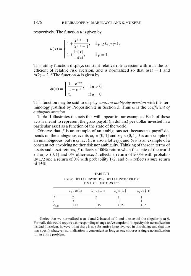
Table II illustrates the acts that will appear in our examples. Each of theseacts is meant to represent the gross payoff (in dollars) per dollar invested in aparticular asset as a function of the state of the world.
Observe that f is an example of an ambiguous act, because its payoff de-pends on the ambiguous events ω1 × (01] and ω2 × (01]; l is an example ofan unambiguous, but risky, act (it is also a lottery); and δ115 is an example of aconstant act, involving neither risk nor ambiguity. Thinking of these in terms ofassets and asset returns, f reflects a 100% return when the state of the worlds ∈ ω1 × (01] and 0% otherwise; l reflects a return of 200% with probabil-ity 1/2 and a return of 0% with probability 1/2; and δ115 reflects a sure returnof 15%.
TABLE II
GROSS DOLLAR PAYOFF PER DOLLAR INVESTED FOREACH OF THREE ASSETS
ω1 × (0 12 ] ω1 × ( 1
2 1] ω2 × (0 12 ] ω2 × ( 1
2 1]
f 2 2 1 1l 3 1 3 1δ115 1.15 1.15 1.15 1.15
11Notice that we normalized u at 1 and 2 instead of 0 and 1 to avoid the singularity at 0.Formally this would require a corresponding change to Assumption 1 to specify this normalizationinstead. It is clear, however, that there is no substantive issue involved in this change and that onemay specify whatever normalization is convenient as long as one chooses a single normalizationfor an entire problem.
DECISION MAKING UNDER AMBIGUITY 1877
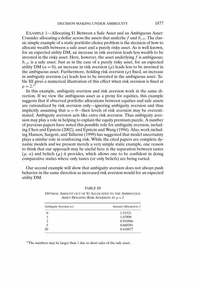
EXAMPLE 1—Allocating $1 Between a Safe Asset and an Ambiguous Asset:Consider allocating a dollar across the assets that underlie f and δ115. The clas-sic simple example of a static portfolio choice problem is the decision of how toallocate wealth between a safe asset and a purely risky asset. As is well known,for an expected utility DM, an increase in risk aversion leads less wealth to beinvested in the risky asset. Here, however, the asset underlying f is ambiguous;δ115 is a safe asset. Just as in the case of a purely risky asset, for an expectedutility DM (α= 0), an increase in risk aversion (ρ) leads less to be invested inthe ambiguous asset. Furthermore, holding risk aversion (ρ) fixed, an increasein ambiguity aversion (α) leads less to be invested in the ambiguous asset. Ta-ble III gives a numerical illustration of this effect when risk aversion is fixed atρ= 2.12
In this example, ambiguity aversion and risk aversion work in the same di-rection. If we view the ambiguous asset as a proxy for equities, this examplesuggests that if observed portfolio allocations between equities and safe assetsare rationalized by risk aversion only—ignoring ambiguity aversion and thusimplicitly assuming that α = 0—then levels of risk aversion may be overesti-mated. Ambiguity aversion acts like extra risk aversion. Thus ambiguity aver-sion may play a role in helping to explain the equity premium puzzle. A numberof previous papers have noted this possible role for ambiguity aversion, includ-ing Chen and Epstein (2002), and Epstein and Wang (1994). Also, work includ-ing Hansen, Sargent, and Tallarini (1999) has suggested that model uncertaintyplays a similar role in reinforcing risk. While the cited papers are complete dy-namic models and we present merely a very simple static example, one reasonto think that our approach may be useful here is the separation between tastes(ρ, α) and beliefs (µ) it provides, which allows one to be confident in doingcomparative statics where only tastes (or only beliefs) are being varied.
Our second example will show that ambiguity aversion does not always pushbehavior in the same direction as increased risk aversion would for an expectedutility DM.
TABLE III
OPTIMAL AMOUNT OUT OF $1 ALLOCATED TO THE AMBIGUOUSASSET HOLDING RISK AVERSION AT ρ= 2
Ambiguity Aversion (α) Amount Allocated to f
0 1.315211 1.078092 0.9169665 0.660381
20 0.418877
12The numbers may be larger than 1 due to short sales of the safe asset.
1878 P. KLIBANOFF, M. MARINACCI, AND S. MUKERJI
EXAMPLE 2—Allocating $1 Between a Safe Asset, a Risky Asset, and an Am-biguous Asset: Here we consider the allocation problem where the risky (butunambiguous) asset that underlies l is available in addition to the ambiguousand safe assets of the previous example. Notice that l has a higher expectedreturn than f . For an expected utility DM, as risk aversion increases, the agentwill want to diversify into both the safe asset and the ambiguous asset f (sinceit is not perfectly correlated with l), trading off expected return against risk.In particular, the ratio of holdings of f to l increases. On the other hand, asambiguity aversion increases, holding risk aversion fixed, the ambiguity aboutthe payoff from f drives the agent away from it as f becomes a less effective di-versifier and less valuable. Hence the ratio of holdings of f to l decreases. Riskaversion and ambiguity aversion are working in opposite directions in terms ofthe composition of the risky part of the agent’s portfolio. Tables IV and V givenumerical illustrations of these effects.13,14
In this case, if such behavior is examined, ignoring ambiguity aversion, notonly will the amount allocated to the safe asset seem to indicate higher riskaversion, as in the previous example, but an examination of the mix of riskyassets (ratio of holdings of f to l) would appear to reveal a lower level of riskaversion than the agent possesses. This suggests that ambiguity may play a rolein explaining the underdiversification puzzle—the finding that the portfoliosof risky assets that individuals hold are not diversified as much as plausiblelevels of risk aversion say they should be. Note that such a story relies on the
TABLE IV
OPTIMAL AMOUNT OUT OF $1 ALLOCATED TO THE RISKY (l) ANDAMBIGUOUS (f ) ASSETS AS RISK AVERSION INCREASES
ASSUMING AMBIGUITY NEUTRALITY (α= 0)
Risk Amount Amount RatioAversion (ρ) Allocated to l Allocated to f f/l
0.75 4.47151 2.07989 0.465141.25 2.36052 1.86083 0.788312 1.19612 1.2136 1.01465 0.357606 0.444743 1.2437
20 0.0761992 0.102747 1.3484
13It is worth noting that the direction of these numerical comparative statics on the ratio ofholdings of f to l as ambiguity aversion increases is unchanged when the safe asset is elimatedfrom this example, when f rather than l has the higher average payoff (switch the 3’s and 2’s), orwhen f and l yield the same average payoff (replace the 3’s with 2’s). However the risk aversionresult for EU is sensitive to the direction of diversification. If f and l have the same expectedreturn, then the ratio is constant in risk aversion under EU. If f has the higher expected return,risk aversion in EU pushes the ratio toward l just as ambiguity aversion does, so that this casewould be similar to the first portfolio example.
14The numbers in a row may sum to more than 1 due to short sales of the safe asset.
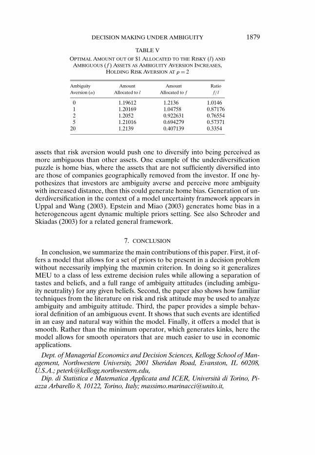
DECISION MAKING UNDER AMBIGUITY 1879
TABLE V
OPTIMAL AMOUNT OUT OF $1 ALLOCATED TO THE RISKY (l) ANDAMBIGUOUS (f ) ASSETS AS AMBIGUITY AVERSION INCREASES,
HOLDING RISK AVERSION AT ρ= 2
Ambiguity Amount Amount RatioAversion (α) Allocated to l Allocated to f f/l
0 1.19612 1.2136 1.01461 1.20169 1.04758 0.871762 1.2052 0.922631 0.765545 1.21016 0.694279 0.57371
20 1.2139 0.407139 0.3354
assets that risk aversion would push one to diversify into being perceived asmore ambiguous than other assets. One example of the underdiversificationpuzzle is home bias, where the assets that are not sufficiently diversified intoare those of companies geographically removed from the investor. If one hy-pothesizes that investors are ambiguity averse and perceive more ambiguitywith increased distance, then this could generate home bias. Generation of un-derdiversification in the context of a model uncertainty framework appears inUppal and Wang (2003). Epstein and Miao (2003) generates home bias in aheterogeneous agent dynamic multiple priors setting. See also Schroder andSkiadas (2003) for a related general framework.
7. CONCLUSION
In conclusion, we summarize the main contributions of this paper. First, it of-fers a model that allows for a set of priors to be present in a decision problemwithout necessarily implying the maxmin criterion. In doing so it generalizesMEU to a class of less extreme decision rules while allowing a separation oftastes and beliefs, and a full range of ambiguity attitudes (including ambigu-ity neutrality) for any given beliefs. Second, the paper also shows how familiartechniques from the literature on risk and risk attitude may be used to analyzeambiguity and ambiguity attitude. Third, the paper provides a simple behav-ioral definition of an ambiguous event. It shows that such events are identifiedin an easy and natural way within the model. Finally, it offers a model that issmooth. Rather than the minimum operator, which generates kinks, here themodel allows for smooth operators that are much easier to use in economicapplications.
Dept. of Managerial Economics and Decision Sciences, Kellogg School of Man-agement, Northwestern University, 2001 Sheridan Road, Evanston, IL 60208,U.S.A.; [email protected],
Dip. di Statistica e Matematica Applicata and ICER, Università di Torino, Pi-azza Arbarello 8, 10122, Torino, Italy; [email protected],
1880 P. KLIBANOFF, M. MARINACCI, AND S. MUKERJI
andDept. of Economics, University of Oxford, Manor Road Building, Manor Road,
Oxford OX1 3UQ, U.K.; and ICER, Torino, Italy; [email protected].
Manuscript received April, 2003; final revision received May, 2005.
APPENDIX: PROOFS AND RELATED MATERIAL
A.1. Preliminaries
Denote by∫ψdϕ(π) the standard Choquet integral, i.e.,
∫ψdϕ(π)=
∫ +∞
0ϕ(π(ψ≥ t))dt +
∫ 0
−∞
(1 −ϕ(π(ψ≥ t)))dt
w.r.t. the set function ϕ(π) :Σ→ [01] induced by a continuous and nonde-creasing function ϕ : [01] → R.
LEMMA 5: Given a continuous and nondecreasing function ϕ : [01] → R anda ψ ∈ B(Σ), the map
π →∫ψdϕ(π)
from ∆ to R, is σ(∆)-measurable.
PROOF: The case ϕ(x)= x for each x ∈ [01] is a standard result (see, e.g.,Aliprantis and Border (1999, p. 483)). Let ϕ : [01] → R be any continuousand nondecreasing function. Given ψ ∈ B(Σ), let Iψ :∆→ R and Lψ :∆→ R
be given by Iψ(π) = ∫ψdϕ(π) and Lψ(π) = ∫
ψdπ, respectively. Supposefirst that ψ= 1E for E ∈ Σ. In this case I1E(π)= ϕ(π(E)) and L1E (π)= π(E),and so I1E = ϕ L1E . Hence, I1E is σ(∆)-measurable since L1E is.
Now, suppose ψ is a simple Σ-measurable function. Then ψ can be writtenas ψ= α0 + ∑n
i=1 αi1Ei with αini=1 ⊆ R+ and E1 ⊆ · · · ⊆ En. Hence,
Iψ(π)=∫ψdϕ(π)= α0 +
n∑i=1
αiϕ(π(Ei))
= α0 +n∑i=1
αiI1Ei (π) ∀π ∈ ∆
and so Iψ is σ(∆)-measurable since each I1Ei is.Finally, suppose ψ is any function in B(Σ). Then there exists a sequence
ψnn of simple Σ-measurable functions that uniformly converge to ψ. Hence,
DECISION MAKING UNDER AMBIGUITY 1881
limn Iψn(π) = Iψ(π) for each π ∈ ∆ and so Iψ is σ(∆)-measurable since each
Iψn is. Q.E.D.
The lottery act lf (π) of Lemma 1 is constructed as follows: define a Borelprobability measure ρ :B → [01] by ρ(B) = πf(B ∩ C) for all Borel subsetsof R and set
F(x)= ρ((−∞x]) for all x ∈ R
Define its generalized inverse F−1 : (01] → R by
F−1(r)= infx ∈ R :F(x)≥ r for each r ∈ (01]Since f is bounded, supp(πf )= supp(ρ) is a compact subset of R and so F−1(r)is well defined for all r ∈ (01]. The desired lottery lf (π) is then given bylf (π)(ω r)= F−1(r) for each r ∈ (01] and each ω ∈Ω.
For example, consider a simple act f , that is, an act taking on a finite num-ber of values. In this case, supp(πf ) is finite, say supp(πf )= x1 xn, withx1 < · · ·< xn. It is easily seen that here lf (π) is given by
lf (π)(ω r)= F−1(r)
=
x1 if r ∈ (0πf (x1)],x2 if r ∈ (πf (x1)πf (x2)+πf(x1)],
xn if r ∈(n−1∑i=1
πf(xi)
n∑i=1
πf(xi)= 1
]
for each r ∈ (01] and each ω ∈Ω.
PROOF OF LEMMA 1: For each x ∈ R we have F−1(r) ≤ x if and only ifF(x)≥ r, so that
λ(r ∈ (01] :F−1(r)≤ x) = λ((0F(x)]) = F(x)= ρ((−∞x])
In turn, this implies λ(r ∈ (01] :F−1(r) ∈ B)= ρ(B) for all B ∈ B, and so
λ(r ∈ (01] :F−1(r) ∈ B) = πf(B) for all B ∈ Bc
(see, e.g., Aliprantis and Border (1999, p. 611)). We conclude that the desiredlottery act lf (π) is given by lf (ω r)= F−1(r) for each r ∈ (01] and eachω ∈Ω(notice that F−1 is nondecreasing and so it is Riemann integrable). Q.E.D.
1882 P. KLIBANOFF, M. MARINACCI, AND S. MUKERJI
A.2. Representation Theorem
We state the more comprehensive representation result mentioned right af-ter Theorem 1 in which the assumptions are both necessary and sufficient.
THEOREM 4: Let and 2 be two binary relations on F and F, respectively.The following statements are equivalent:
(i) Assumptions 1, 2, and 3 hold.(ii) There exists a continuous, strictly increasing φ :U → R, a unique count-
ably additive probability µ :σ(∆)→ [01], and continuous and strictly increasingutility functions v :C → R and u :C → R such that
(a) φ= v u−1;(b) 2 is represented by the preference functional V 2 :F → R given by
V 2(f)=∫∆
v(f)dµ;
(c) is represented by the preference functional V :F → R given by
V (f )=∫Uφ(x)dµf =
∫∆
φ
[∫S
u(f )dπ
]dµ≡ Eµφ(Eπu f )
Moreover, v and u are unique up to positive affine transformations, and if u=αu+β, α> 0, then the associated φ is such that φ(αy+β)=φ(y), where y ∈ U .
A.3. Results on Ambiguity Attitude
PROOF OF LEMMA 2: First notice that, since both C and U are Borel sub-sets of R, both Bc and Bu coincide with the restrictions of the Borel σ-algebraof R on C and U , respectively. Since u is injective and Borel measurable,each set u(B), with B ∈ Bc , belongs to Bu (see, e.g., Corollary 15.2 of Kechris(1995)). Hence, u(B) :B ∈ Bc ⊆ Bu. On the other hand, let B ∈ Bu. Since u isBorel measurable, u−1(B) ∈ Bc . Hence, B= u(u−1(B)) ∈ u(B) :B ∈ Bc, as de-sired. Q.E.D.
We next state a lemma (see Theorems 88 and 91 in Hardy, Littlewood, andPolya (1952)) useful in several proofs to follow.
LEMMA 6: Let φ :A⊆ R → R be a continuous function defined on a convexset A. Then φ is concave (strictly concave) if and only if there exists λ ∈ (01)such that, for all x y ∈A with x = y ,
φ(λx+ (1 − λ)y)≥ (>) λφ(x)+ (1 − λ)φ(y)(11)
DECISION MAKING UNDER AMBIGUITY 1883
PROOF OF PROPOSITION 1: Part (i) implies (iii): By the Jensen inequality,φ(
∫xdµΠf )≥ ∫
φ(x)dµΠf . Thus, φ(e(µΠf ))≥ ∫φ(x)dµΠf , which in turn
implies δu−1(e(µΠf ))Π f by Theorem 1.
Part (iii) implies (i): SupposeΠ consists of two mutually singular probabilitymeasures π ′ and π ′′, i.e., there is some event E with π ′(E)= 1 and π ′′(E)= 0.Given any x y ∈ U , let a = u−1(x) and b = u−1(y). Hence, ab ∈ C and sof ≡ aEb ∈ F . Then u(cf (π ′))= u(a)= x and u(cf (π ′′))= u(b)= y . Since, bydefinition, µΠ has full support on Π, there is λ ∈ (01) such that µΠ(π ′) = λand µΠ(π ′′) = 1 − λ. Thus, µΠf (x) = λ and µΠf (y) = 1 − λ. By (iii) and therepresentation,
φ(λx+ (1 − λ)y)≥ λφ(x)+ (1 − λ)φ(y)(12)
so there exists λ ∈ (01) such that, given any x y ∈ U , (12) holds. By Lemma 6,φ is concave. Finally, by Assumption 4, φ is independent of the choice of Πabove.
That part (i) is equivalent to (ii) follows from the fact that φ = v u−1 andthus v=φ u up to a positive affine transformation. Q.E.D.
PROOF OF THEOREM 2: The “if” part follows easily from the Jensen in-equality.
As to the “only if” part, we first show that A and B share the same vN–Mutility function u. Let L∗ be the set of all lottery acts that are step functionsof the form
∑n
i=1 xi1(ri−1ri], with r0 = 0, rn = 1, xi ∈ C for each i= 1 n, andx1 < · · ·< xn. Such lottery acts are in one-to-one correspondence with simpleprobability measures p on C, i.e., measures such that p(A)= 1 for some finiteset A⊆ C. In fact, each such p induces a unique lp ∈L∗ given by
lp(ω r)=
x1 if r ∈ (0p(x1)],x2 if r ∈ (
p(x1)p(x2)+p(x1)],
xn if r ∈(n−1∑i=1
p(xi)
n∑i=1
p(xi)= 1
],
where x1 xn is the support of p, with x1 < · · ·< xn. On the other hand,each l ∈ L∗ induces a unique simple probability measure pl on C with supportx1 xn given by p(xi)= λ(l−1(xi)) for each i= 1 n.
Let P be the set of all simple probability measures on C. Define AΠ on P by
pAΠ q ⇐⇒ lp A
Π lq(13)
In a similar way, define BΠ on P . Both A
Π and BΠ are well defined by what
was just observed. Moreover, defineUA :P → R byUA(p)= ∑x∈supp(p) uA(x)×
1884 P. KLIBANOFF, M. MARINACCI, AND S. MUKERJI
p(x), where uA is the vN–M utility index given by Assumption 1. In a similarway, define UB :P → R.
Clearly, UA(p) = ∫(01] u(lp(r))dr for all p ∈ P , and so Assumption 1
and (13) imply that pAΠ q if and only if UA(p)≥UA(q) for all pq ∈P .
Let l l′ ∈L∗. By (7),
l AΠ l
′ ⇒ l BΠ l
′
Hence, for all pq ∈P ,
pAΠ q ⇒ pB
Π q
Since UA and UB are nonconstant affine functionals on P , by Corollary B.3of Ghirardato, Maccheroni, and Marinacci (2004) there exist α > 0 and β ∈ R
such that UA = αUB +β. Hence, uA = αuB +β. Along with the normalizationuA(0)= uB(0)= 0 and uA(1)= uB(1)= 1, this implies uA = uB, as desired.
Set u = uA = uB and h(x) = (φA φ−1B )(x) for all x ∈ U . The function h is
clearly strictly increasing. Moreover, since (φ−1A φA)(x)= x= (φ−1
B φB)(x)for all x ∈ U , we have φA = h φB. We want to show that h is concave if andonly if A is more ambiguity averse than B.
By Definition 5,∫φA dµf ≥ φA(u(x)) implies
∫φB dµf ≥ φB(u(x)) for all
f ∈ F and x ∈ C. Since U is an interval, given any f ∈ F there exists xf ∈ Csuch that
∫φA dµf = φA(u(xf )). Hence, f ∼1 δxf and so, by (7),
∫φB dµf ≥
φB(u(xf )). In turn this implies that, for all f ∈F ,
φ−1B
(∫φB dµf
)≥φ−1
A
(∫φA dµf
)
and so
h
(∫φB dµf
)≥
∫φA dµf =
∫(h φB)dµf (14)
Let φB(x)φB(y) ∈ φB(U). By proceeding as in the proof of Proposition 1,there is a set Π, an act f , and a λ ∈ (01) such that µΠf (x)= λ and µΠf (y)=1 − λ. Hence, (14) reduces to
h(λφ(x)+ (1 − λ)φ(y)) ≥ λh(φ(x))+ (1 − λ)h(φ(y))
Since φB(U) is an interval, by Lemma 6 we conclude that h is concave.Q.E.D.
PROOF OF PROPOSITION 2: Without loss of generality, assume that U =[01]. Let k ∈ (01) and set Uk = [01−k]. Let Ck ⊆ C be such that u(Ck)= Ukand consider
Fk = f ∈F : f (s) ∈ Ck for each s ∈ S
DECISION MAKING UNDER AMBIGUITY 1885
Define kΠ on Fk as f k
Π g if and only if
∫φk
(∫u(f (s))dπ
)dµΠ ≥
∫φk
(∫u(g(s))dπ
)dµΠ
where φk(x) = φ(x + k) for each x ∈ Uk. For any f ∈ Fk, l ∈ L ∩ Fk andcorresponding f ′ and l′ as in Definition 6, we have
f kΠ l ⇐⇒
∫φk
(∫u(f (s))dπ
)dµΠ ≥φk
(∫(01]
u(l(r))dr
)
⇐⇒∫φ
(∫ (u(f (s))+ k)
dπ
)dµΠ
≥φ(∫
(01]
(u(l(r))+ k)
dr
)
⇐⇒∫φ
(∫u(f ′(s))dπ
)dµΠ ≥φ
(∫(01]
u(l′(r))dr)
⇐⇒ f ′ Π l′ ⇐⇒ f Π l
where the last equivalence follows from Definition 6. Hence, k is as ambiguityaverse as when restricted to Fk. By Theorem 2, there exist a(k) > 0 andb(k) ∈ R such that, for all x ∈ [01 − k],
φ(x+ k)=φk(x)= a(k)φ(x)+ b(k)(15)
Since k was arbitrary, we conclude that the functional equation (15) holdsfor all k ∈ (01) and all x ∈ (01) such that x + k ≤ 1. This is a variation ofCauchy’s functional equation (see p. 150 of Aczel (1966)), and its only strictlyincreasing solutions are (up to positive affine transformations) φ(x) = x orφ(x)= − 1
αe−αx, α = 0. Q.E.D.
PROOF OF PROPOSITION 3: We begin with a couple of lemmas. The first oneis proved in Maccheroni, Marinacci, and Rustichini (2004), and is a variationon a result of Donsker and Varadhan (see, e.g., Proposition 1.4.1 of Dupuisand Ellis (1997)).
LEMMA 7: Given any bounded σ(∆)-measurable function ψ :∆→ R and anyfinitely additive probability measure η on σ(∆), we have
limn→+∞
−1n
log∫∆
e−nψ dη= ess infψ
1886 P. KLIBANOFF, M. MARINACCI, AND S. MUKERJI
Observe that, if we set φn(x)= −e−nx for all x ∈ψ(∆), we can write
φ−1n
(∫∆
φn(ψ)dη
)= −1
nlog
∫∆
e−nψ dη
where φ−1n (x) = −(1/n) log(−x) for all x ∈ φn(ψ(∆)) ⊆ (−∞0). Next we
generalize Lemma 7 to general sequences of functions φn.
LEMMA 8: Let ψ be a bounded σ(∆)-measurable function ψ :∆→ R and letη be a finitely additive probability measure on σ(∆). Suppose φnn is a sequenceof real-valued functions φn : I → R defined on an interval I of R with Arrow–Pratt coefficients αn : I → R such that limn→∞(infx∈I αn(x))= +∞ and αn(x) ≤αn+1(x) for each x ∈ I and each n. Then
limn→+∞
φ−1n
(∫∆
φn(ψ)dη
)= ess infψ(16)
PROOF: Given any strictly increasing function χ : I → R, we have∫∆χ(ψ)×
dη≥ χ(ess infψ) and so
χ−1
(∫∆
χ(ψ)dη
)≥ ess infψ(17)
Now let χ1 : I → R and χ2 : I → R be any two concave and strictly increasingfunctions with Arrow–Pratt coefficients α1 and α2 such that α1(x)≥ α2(x) foreach x ∈ I. Since I is an interval and α1 ≥ α2, by Theorem 1 of Pratt (1964) thefunction (χ1 χ−1
2 )(t) is concave in t. Hence, by the Jensen inequality,∫∆
χ1(ψ)dη=∫∆
(χ1 χ−12 χ2)(ψ)dη=
∫∆
(χ1 χ−12 )(χ2(ψ))dη
≤ (χ1 χ−12 )
(∫∆
χ2(ψ)dη
)
so that, being χ1 strictly increasing,
χ−11
(∫∆
χ1(ψ)dη
)≤ χ−1
2
(∫∆
χ2(ψ)dη
)(18)
In particular, given any m and n with m> n, (18) implies
φ−1m
(∫∆
φm(ψ)dη
)≤φ−1
n
(∫∆
φn(ψ)dη
)(19)
Hence, limn→+∞φ−1n (
∫∆φn(ψ)dη) exists.

DECISION MAKING UNDER AMBIGUITY 1887
By (17) with χ(x) = −e−nx, we have − 1n
log∫∆e−nψ dη ≥ ess infψ for each
n≥ 1. Hence, given any ε > 0, by Lemma 7 there is nε ≥ 1 such that
− 1nε
log∫∆
exp(−nεψ)dη− ess infψ≤ ε
Since limn→∞(infx∈U αn(x))= +∞, there exists nε ≥ 1 such that infx∈U αn(x)≥ nεfor each n ≥ nε. Hence, if n ≥ nε, the Arrow–Pratt coefficient αn of each φnis larger than nε, which is the Arrow–Pratt coefficient of −exp(−nεx). As aresult, (18) implies
φ−1n
(∫∆
φn(ψ)dη
)≤ − 1
nεlog
∫∆
exp(−nεψ)dη ∀n≥ nε
and so
φ−1n
(∫∆
φn(ψ)dη
)− ess infψ
≤ − 1nε
log∫∆
exp(−nεψ)dη− ess infψ≤ ε ∀n≥ nε
Since ε was arbitrary, this implies
limn→+∞
φ−1n
(∫∆
φn(ψ)dη
)≤ ess infψ
On the other hand, since each φn : I → R is strictly increasing, by (17) wehave φ−1
n (∫∆φn(ψ)dη) ≥ ess infψ for each n ≥ 1 and we conclude that (16)
holds. Q.E.D.
We can now prove Proposition 3. Let AnΠ be the orderings on F that
share the same measures µΠ . Since, for all n, An+1 is more ambiguity aversethanAn, Theorem 2 implies that all the An
Π share the same vN–M utility func-tion u. Given fg ∈ F , set F(π)= ∫
u(f )dπ and G(π)= ∫u(g)dπ for each
π ∈ ∆. Since u(f ), u(g) are in B(Σ), by Lemma 5 both F and G are boundedσ(∆)-measurable functions. Suppose that, for some n0, f An
Π g for eachn≥ n0. Set φn =φAn . By Theorem 1,∫
∆
φn(F(π))dµΠ ≥∫∆
φn(G(π))dµΠ ∀n≥ n0
and so
φ−1n
(∫∆
φn(F(π))dµΠ
)≥φ−1
n
(∫∆
φn(G(π))dµΠ
) ∀n≥ n0
1888 P. KLIBANOFF, M. MARINACCI, AND S. MUKERJI
Since U is an interval, we can apply Lemma 8 and so we have ess infΠ F ≥ess infΠ G, as desired.
To complete the proof, suppose ess infΠ F > ess infΠ G. By Lemma 8, thereexists n0 large enough so that, for all n≥ n0,∣∣∣∣φ−1
n
(∫∆
φn(G(π))dµΠ
)− ess infΠ G
∣∣∣∣< ess infΠ F − ess infΠ G2
Hence, since φ−1n (
∫∆φn(F(π))dµΠ)≥ ess infΠ F ,
φ−1n
(∫∆
φn(F(π))dµΠ
)
>φ−1n
(∫∆
φn(G(π))dµΠ
) for all n≥ n0
which in turn implies f AnΠ g for all n≥ n0. Q.E.D.
PROOF OF LEMMA 3: Suppose f is upper semicontinuous. As u is contin-uous, then u(f ) as well is upper semicontinuous. Then the map π → Eπu(f )is upper semicontinuous in the vague topology of ∆ (see, e.g., Theorem 14.5in Aliprantis and Border (1999)). Clearly, µ(Eπu(f ) ≥ ess infΠ Eπu(f )) = 1.Since the map π → Eπu(f ) is upper semicontinuous, the set (Eπu(f ) ≥ess infΠ Eπu(f )) is closed in ∆ and so by the definition of support we haveΠ ⊆ (Eπu(f ) ≥ ess infΠ Eπu(f )). Hence, infΠ Eπu(f ) ≥ ess infΠ Eπu(f ). Onthe other hand, µ(Eπu(f ) < infΠ Eπu(f )) ≤ µ(Πc) = 0 and so, by the de-finition of ess infΠ Eπu(f ), infΠ Eπu(f ) ≤ ess infΠ Eπu(f ). We conclude thatinfΠ Eπu(f )= ess infΠ Eπu(f ), as desired.
Finally, if f is continuous and Π is compact, then the map π → Eπu(f ) iscontinuous on a compact set and so by the Weierstrass theorem it attains aminimum on Π. Q.E.D.
PROOF OF PROPOSITION 4: To prove part 1, apply Proposition 1 and its ana-logue for smooth ambiguity love, and note that φ both concave and convexis equivalent to φ linear. Now turn to the proof of part 2, where φ strictlyconcave on an open interval J ⊆ U implies φ(
∫xdµΠf ) >
∫φ(x)dµΠf for all
µΠf with nonsingleton supp(µΠf )⊆ J by the strict version of Jensen’s inequal-ity. Thus φ(e(µΠf )) >
∫φ(x)dµΠf , which in turn implies δu−1(e(µΠ))
Π f forall (fΠ) with nonsingleton supp(µΠf ) ⊆ J by Theorem 1. The reverse di-rection follows directly from the argument in the proof of Proposition 1 thatsmooth ambiguity aversion implies concavity of φ with the weak inequali-ties replaced by strict and attention limited to x y ∈ J ⊆ U . Part 3 followsexactly as 2 with concavity replaced by convexity, inequalities reversed, andx y ∈K ⊆ U . Q.E.D.
DECISION MAKING UNDER AMBIGUITY 1889
PROOF OF LEMMA 4: Suppose φ :U → R is twice continuously differen-tiable and is not linear. There exists x0 ∈ U such that φ′′(x0) = 0. Supposeper contra that φ′′(x) = 0 for all x ∈ U . Then φ′(x) = k ∈ R for all x ∈ U .Hence, φ(x) = kx + c for some k c ∈ R, a contradiction. We conclude thatthere is x0 ∈ U such that φ′′(x0) = 0. Since φ′′ is continuous, there exists an in-terval (αβ)⊆ U , with x0 ∈ [αβ], such thatφ′′(x)φ′′(x0) > 0 for all x ∈ (αβ),which implies the desired conclusion. Q.E.D.
A.4. Results on Ambiguity
PROOF OF PROPOSITION 5: Suppose (9) holds. Let E be such that xEy xBy . By Theorem 1, V (xBy)=φ(u(x)β+ u(y)(1 −β)), where β= π(B) forall π ∈Π. Since φ(u(y))≤ V (xEy)≤φ(u(x)), by the continuity of φ there isβ∗ ≥ β such that
φ(u(x)β∗ + u(y)(1 −β∗)
) = V (xEy)(20)
Since λ is nonatomic, there is Ω × B1 B∗ ⊇ B such that π(B∗) = β∗ forall π ∈Π. Hence, by (20) and by Theorem 1, xEy ∼ xB∗y . By (9), this impliesthat yEx∼ yB∗x. Whereasφ is strictly increasing,φ(u(x)(1−β∗)+u(y)β∗) <φ(u(x)(1 − β) + u(y)β) and so, by Theorem 1, yB∗x ≺ yBx. Hence, yEx ≺yBx and we conclude that
xEy xBy ⇒ yEx≺ yBxA similar argument proves the converse implication and so
xEy xBy ⇐⇒ yEx≺ yBxFinally, again a similar argument shows that
xEy ≺ xBy ⇐⇒ yEx yBxas desired. This completes the proof because the “only if” part is trivial.
Q.E.D.
PROOF OF THEOREM 3: By assumption, satisfies the conditions in Theo-rem 1 and so the representation there applies. Fix an eventE ∈ Σ. Suppose thatE is ambiguous. This means that there exists an event B ∈ Ω×B1 and x y ∈ Cwith δx δy such that either [xEy xBy and yEx yBx] or [xEy ≺ xBy andyEx yBx] or [xEy ∼ xBy and yEx yBx]. Let β denote π(B) (which is thesame for all π ∈ ∆). If π(E) were equal to some fixed α ∈ [01] for µ-almost-allπ, then, by the representation, for all wz ∈ C,
wEz wBz ⇐⇒ αu(w)+ (1 − α)u(z)≥ βu(w)+ (1 −β)u(z)
1890 P. KLIBANOFF, M. MARINACCI, AND S. MUKERJI
However, this makes it impossible for E to be ambiguous. Therefore π(E)must vary across ∆. Specifically, if γ = ∫
∆π(E)dµ, then there exist µ-nonnull
sets Π′ ∈ σ(∆) and Π′′ ∈ σ(∆) such that π(E) < γ for π ∈Π′ and π(E) > γfor π ∈Π′′, and the first claim in the theorem is proved.
Next, suppose that are not smoothly ambiguity neutral, Assumptions4 and 5 hold and E is unambiguous. Proposition 4 implies that φ is strictly con-cave (or strictly convex) on a nonempty open interval (u1u2)⊆ U . Fix k l ∈ Usuch that u1 <k< l < u2. Let γ = ∫
∆π(E)dµOne can think of γ as the DM’s
“expected” probability of the event E. According to our representation of pref-erences, the following equalities are true:
V(u−1(l)Ω × (0γ]u−1(k)
) =φ(γl+ (1 − γ)k)V
(u−1(l)Eu−1(k)
) =∫∆
φ(π(E)l+ (1 −π(E))k)
dµ
V(u−1(k)Ω × (0γ]u−1(l)
) =φ(γk+ (1 − γ)l)V
(u−1(k)Eu−1(l)
) =∫∆
φ(π(E)k+ (1 −π(E))l)dµ
Since φ is strictly concave (the strictly convex case follows similarly) on theinterval [k l], Jensen’s inequality (and the definition of γ) implies that
V(u−1(l)Eu−1(k)
) ≤ V (u−1(l)Ω × (0γ]u−1(k)
)and
V(u−1(k)Eu−1(l)
) ≤ V (u−1(k)Ω × (0γ]u−1(l)
)with both inequalities strict if it is not the case that π(E) takes on the samevalue everywhere (specifically, π(E) = γ for µ-almost-all π). Suppose thatboth inequalities are indeed strict. This says that
u−1(l)Eu−1(k)≺ u−1(l)Ω × (0γ]u−1(k)
and
u−1(k)Eu−1(l)≺ u−1(k)Ω × (0γ]u−1(l)
implying that E is ambiguous, a contradiction. Therefore, it must be thatπ(E) = γ µ-almost-everywhere and the second claim in the theorem isproved. Q.E.D.
REFERENCES
ACZEL, J. (1966): Lectures on Functional Equations and Their Applications. New York: AcademicPress.
DECISION MAKING UNDER AMBIGUITY 1891
ALIPRANTIS, C., AND K. BORDER (1999): Infinite Dimensional Analysis. Berlin: Springer-Verlag.ARROW, K. J. (1971): Essays in the Theory of Risk-Bearing. Chicago: Markham.CHEN, Z., AND L. G. EPSTEIN (2002): “Ambiguity, Risk, and Asset Returns in Continuous Time,”
Econometrica, 70, 1403–1443.CHEW, H. S., AND J. S. SAGI (2003): “Small Worlds: Modeling Attitudes Towards Sources of
Uncertainty,” Mimeo, available at http://faculty.haas.berkeley.edu/sagi/03SmallWorlds.pdf.DUPUIS, P., AND R. S. ELLIS (1997): A Weak Convergence Approach to the Theory of Large Devia-
tions. New York: John Wiley & Sons.ELLSBERG, D. (1961): “Risk, Ambiguity, and the Savage Axioms,” Quarterly Journal of Eco-
nomics, 75, 643–669.EPSTEIN, L. G. (1999): “A Definition of Uncertainty Aversion,” Review of Economic Studies, 66,
579–608.EPSTEIN, L. G., AND J. MIAO (2003): “A Two-Person Dynamic Equilibrium under Ambiguity,”
Journal of Economic Dynamics and Control, 27, 1253–1288.EPSTEIN, L. G., AND T. WANG (1994): “Intertemporal Asset Pricing under Knightian Uncer-
tainty,” Econometrica, 62, 283–322.EPSTEIN, L. G., AND J. ZHANG (2001): “Subjective Probabilities on Subjectively Unambiguous
Events,” Econometrica, 69, 265–306.EPSTEIN, L. G., AND S. E. ZIN (1989): “Substitution, Risk Aversion, and the Temporal Behavior
of Consumption and Asset Returns: A Theoretical Framework,” Econometrica, 57, 937–969.ERGIN, H., AND F. GUL (2002): “A Subjective Theory of Compound Lotteries,” Discussion Paper,
Princeton University.GHIRARDATO, P., F. MACCHERONI, AND M. MARINACCI (2004): “Differentiating Ambiguity and
Ambiguity Attitude,” Journal of Economic Theory, 118, 133–173.GHIRARDATO, P., AND M. MARINACCI (2002): “Ambiguity Made Precise: A Comparative Foun-
dation,” Journal of Economic Theory, 102, 251–289.GILBOA, I., AND D. SCHMEIDLER (1989): “Maxmin Expected Utility with a Non-Unique Prior,”
Journal of Mathematical Economics, 18, 141–153.GRANDMONT, J.-M. (1972): “Continuity Properties of a von Neumann–Morgenstern Utility,”
Journal of Economic Theory, 4, 45–57.GRANT, S., A. KAJII, AND B. POLAK (2001): “Third Down with a Yard to Go: Recursive Expected
Utility and the Dixit–Skeath Conundrum,” Economics Letters, 73, 275–286.HALEVY, Y. (2004): “Ellsberg Revisited: An Experimental Study,” available at http://www.econ.
ubc.ca/halevy.HALEVY, Y., AND V. FELTKAMP (2005): “A Bayesian Approach to Uncertainty Aversion,” Review
of Economic Studies, 72, 449–466.HANSEN, L., AND T. SARGENT (2000): “Wanting Robustness in Macroeconomics,” available at
http://home.uchicago.edu/~lhansen/.HANSEN, L. P., T. J. SARGENT, AND T. D. TALLARINI, JR. (1999): “Robust Permanent Income and
Pricing,” Review of Economic Studies, 66, 873–907.HARDY, G., J. E. LITTLEWOOD, AND G. POLYA (1952): Inequalities. Cambridge, U.K.: Cambridge
University Press.KECHRIS, A. S. (1995): Classical Descriptive Set Theory. New York: Springer-Verlag.KLIBANOFF, P., M. MARINACCI, AND S. MUKERJI (2003): “A Smooth Model of Decision Mak-
ing under Ambiguity,” Discussion Paper 113, Department of Economics, Oxford University,available at http://www.econ.ox.ac.uk/Research/wp/pdf/paper113.pdf.
KREPS, D., AND E. PORTEUS (1978): “Temporal Resolution of Uncertainty and Dynamic ChoiceTheory,” Econometrica, 46, 185–200.
LOOMES, G., AND U. SEGAL (1994): “Observing Orders of Risk Aversion,” Journal of Risk andUncertainty, 9, 239–256.
MACCHERONI, F., M. MARINACCI, AND A. RUSTICHINI (2004): “Variational Representation ofPreferences under Ambiguity,” Mimeo, available at http://web.econ.unito.it/gma/massimo.htm.
1892 P. KLIBANOFF, M. MARINACCI, AND S. MUKERJI
MACHINA, M. (2004): “Almost-Objective Uncertainty,” Economic Theory, 24, 1–54.NAU, R. (2001): “Uncertainty Aversion with Second-Order Probabilities and Utilities,” in Second
International Symposium on Imprecise Probabilities and Their Application. Ithaca, NY, 273–283;available at http://www.sipta.org/~isipta01/proceedings/index.html.
(2003): “Uncertainty Aversion with Second-Order Probabilities and Utilities,” Manage-ment Science, forthcoming.
NEILSON, W. S. (1993): “Ambiguity Aversion: An Axiomatic Approach Using Second Order Prob-abilities,” Mimeo, Texas A&M University.
PRATT, J. W. (1964): “Risk Aversion in the Small and in the Large,” Econometrica, 32, 122–136.QUIGGIN, J. (1993): Generalized Expected Utility Theory: The Rank-Dependent Expected Utility
Model. Dordrecht: Kluwer.SARIN, R., AND P. WAKKER (1992): “A Simple Axiomatization of Nonadditive Expected Utility,”
Econometrica, 60, 1255–1272.(1997): “A Single-Stage Approach to Anscombe and Aumann’s Expected Utility,” Review
of Economic Studies, 64, 399–409.SCHMEIDLER, D. (1989): “Subjective Probability and Expected Utility Without Additivity,”
Econometrica, 57, 571–587.SCHRODER, M., AND C. SKIADAS (2003): “Optimal Lifetime Consumption-Portfolio Strategies
under Trading Constraints and Generalized Recursive Preferences,” Stochastic Processes andTheir Applications, 108, 155–202.
SEGAL, U. (1987): “The Ellsberg Paradox and Risk Aversion: An Anticipated Utility Approach,”International Economic Review, 28, 175–202.
(1990): “Two-Stage Lotteries Without the Reduction Axiom,” Econometrica, 58,349–377.
SEGAL, U., AND A. SPIVAK (1990): “First Order versus Second Order Risk Aversion,” Journal ofEconomic Theory, 51, 111–125.
UPPAL, R., AND T. WANG (2003): “Model Misspecification and under Diversification,” Journal ofFinance, 58, 2465–2486.
WAKKER, P. (1989): Additive Representations of Preferences, a New Foundation of Decision Analysis.Dordrecht: Kluwer.