Study guide: Finite di�erence methods for vibration

problems

Hans Petter Langtangen1,2

Center for Biomedical Computing, Simula Research Laboratory1

Department of Informatics, University of Oslo2

Oct 12, 2015

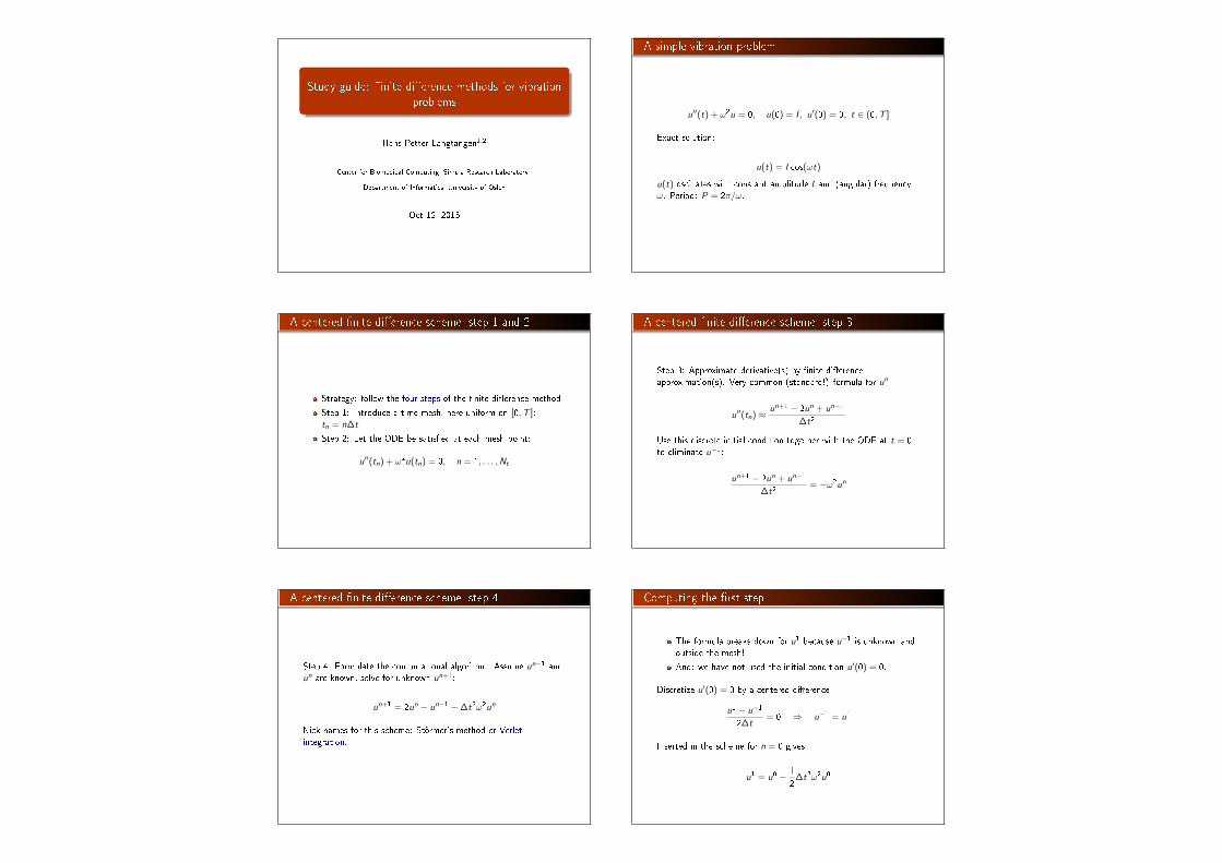
A simple vibration problem

u′′(t) + ω2u = 0, u(0) = I , u′(0) = 0, t ∈ (0,T ]

Exact solution:

u(t) = I cos(ωt)

u(t) oscillates with constant amplitude I and (angular) frequencyω. Period: P = 2π/ω.

A centered �nite di�erence scheme; step 1 and 2

Strategy: follow the four steps of the �nite di�erence method.

Step 1: Introduce a time mesh, here uniform on [0,T ]:tn = n∆t

Step 2: Let the ODE be satis�ed at each mesh point:

u′′(tn) + ω2u(tn) = 0, n = 1, . . . ,Nt

A centered �nite di�erence scheme; step 3

Step 3: Approximate derivative(s) by �nite di�erenceapproximation(s). Very common (standard!) formula for u′′:

u′′(tn) ≈ un+1 − 2un + un−1

∆t2

Use this discrete initial condition together with the ODE at t = 0to eliminate u−1:

un+1 − 2un + un−1

∆t2= −ω2un

A centered �nite di�erence scheme; step 4

Step 4: Formulate the computational algorithm. Assume un−1 andun are known, solve for unknown un+1:

un+1 = 2un − un−1 −∆t2ω2un

Nick names for this scheme: Störmer's method or Verletintegration.

Computing the �rst step

The formula breaks down for u1 because u−1 is unknown andoutside the mesh!

And: we have not used the initial condition u′(0) = 0.

Discretize u′(0) = 0 by a centered di�erence

u1 − u−1

2∆t= 0 ⇒ u−1 = u1

Inserted in the scheme for n = 0 gives

u1 = u0 − 1

2∆t2ω2u0

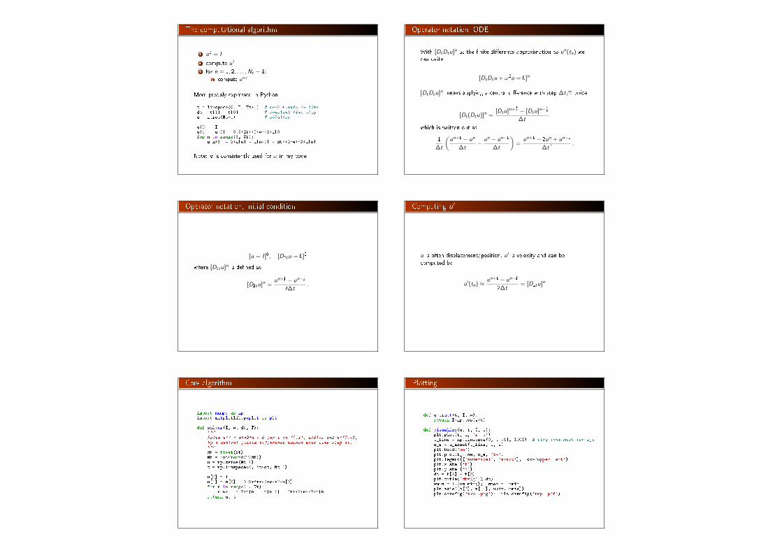
The computational algorithm

1 u0 = I

2 compute u1

3 for n = 1, 2, . . . ,Nt − 1:1 compute un+1

More precisly expressed in Python:

t = linspace(0, T, Nt+1) # mesh points in timedt = t[1] - t[0] # constant time step.u = zeros(Nt+1) # solution

u[0] = Iu[1] = u[0] - 0.5*dt**2*w**2*u[0]for n in range(1, Nt):

u[n+1] = 2*u[n] - u[n-1] - dt**2*w**2*u[n]

Note: w is consistently used for ω in my code.

Operator notation; ODE

With [DtDtu]n as the �nite di�erence approximation to u′′(tn) wecan write

[DtDtu + ω2u = 0]n

[DtDtu]n means applying a central di�erence with step ∆t/2 twice:

[Dt(Dtu)]n =[Dtu]n+ 1

2 − [Dtu]n−1

2

∆t

which is written out as

1

∆t

(un+1 − un

∆t− un − un−1

∆t

)=

un+1 − 2un + un−1

∆t2.

Operator notation; initial condition

[u = I ]0, [D2tu = 0]0

where [D2tu]n is de�ned as

[D2tu]n =un+1 − un−1

2∆t.

Computing u′

u is often displacement/position, u′ is velocity and can becomputed by

u′(tn) ≈ un+1 − un−1

2∆t= [D2tu]n

Core algorithm

import numpy as npimport matplotlib.pyplot as plt

def solver(I, w, dt, T):"""Solve u'' + w**2*u = 0 for t in (0,T], u(0)=I and u'(0)=0,by a central finite difference method with time step dt."""dt = float(dt)Nt = int(round(T/dt))u = np.zeros(Nt+1)t = np.linspace(0, Nt*dt, Nt+1)

u[0] = Iu[1] = u[0] - 0.5*dt**2*w**2*u[0]for n in range(1, Nt):

u[n+1] = 2*u[n] - u[n-1] - dt**2*w**2*u[n]return u, t

Plotting

def u_exact(t, I, w):return I*np.cos(w*t)

def visualize(u, t, I, w):plt.plot(t, u, 'r--o')t_fine = np.linspace(0, t[-1], 1001) # very fine mesh for u_eu_e = u_exact(t_fine, I, w)plt.hold('on')plt.plot(t_fine, u_e, 'b-')plt.legend(['numerical', 'exact'], loc='upper left')plt.xlabel('t')plt.ylabel('u')dt = t[1] - t[0]plt.title('dt=%g' % dt)umin = 1.2*u.min(); umax = -uminplt.axis([t[0], t[-1], umin, umax])plt.savefig('tmp1.png'); plt.savefig('tmp1.pdf')

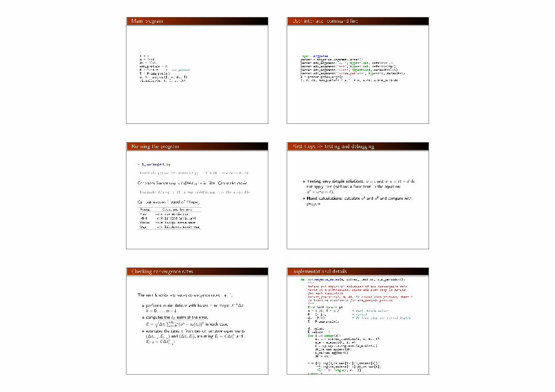
Main program

I = 1w = 2*pidt = 0.05num_periods = 5P = 2*pi/w # one periodT = P*num_periodsu, t = solver(I, w, dt, T)visualize(u, t, I, w, dt)

User interface: command line

import argparseparser = argparse.ArgumentParser()parser.add_argument('--I', type=float, default=1.0)parser.add_argument('--w', type=float, default=2*pi)parser.add_argument('--dt', type=float, default=0.05)parser.add_argument('--num_periods', type=int, default=5)a = parser.parse_args()I, w, dt, num_periods = a.I, a.w, a.dt, a.num_periods

Running the program

vib_undamped.py:

Terminal> python vib_undamped.py --dt 0.05 --num_periods 40

Generates frames tmp_vib%04d.png in �les. Can make movie:

Terminal> ffmpeg -r 12 -i tmp_vib%04d.png -c:v flv movie.flv

Can use avconv instead of ffmpeg.

Format Codec and �lename

Flash -c:v flv movie.flv

MP4 -c:v libx264 movie.mp4

Webm -c:v libvpx movie.webm

Ogg -c:v libtheora movie.ogg

First steps for testing and debugging

Testing very simple solutions: u = const or u = ct + d donot apply here (without a force term in the equation:u′′ + ω2u = f ).

Hand calculations: calculate u1 and u2 and compare withprogram.

Checking convergence rates

The next function estimates convergence rates, i.e., it

performs m simulations with halved time steps: 2−k∆t,k = 0, . . . ,m − 1,

computes the L2 norm of the error,

E =√

∆ti∑Nt−1

n=0 (un − ue(tn))2 in each case,

estimates the rates ri from two consecutive experiments(∆ti−1,Ei−1) and (∆ti ,Ei ), assuming Ei = C∆trii andEi−1 = C∆trii−1:

Implementational details

def convergence_rates(m, solver_function, num_periods=8):"""Return m-1 empirical estimates of the convergence ratebased on m simulations, where the time step is halvedfor each simulation.solver_function(I, w, dt, T) solves each problem, where Tis based on simulation for num_periods periods."""from math import piw = 0.35; I = 0.3 # just chosen valuesP = 2*pi/w # perioddt = P/30 # 30 time step per period 2*pi/wT = P*num_periods

dt_values = []E_values = []for i in range(m):

u, t = solver_function(I, w, dt, T)u_e = u_exact(t, I, w)E = np.sqrt(dt*np.sum((u_e-u)**2))dt_values.append(dt)E_values.append(E)dt = dt/2

r = [np.log(E_values[i-1]/E_values[i])/np.log(dt_values[i-1]/dt_values[i])for i in range(1, m, 1)]

return r

Result: r contains values equal to 2.00 - as expected!

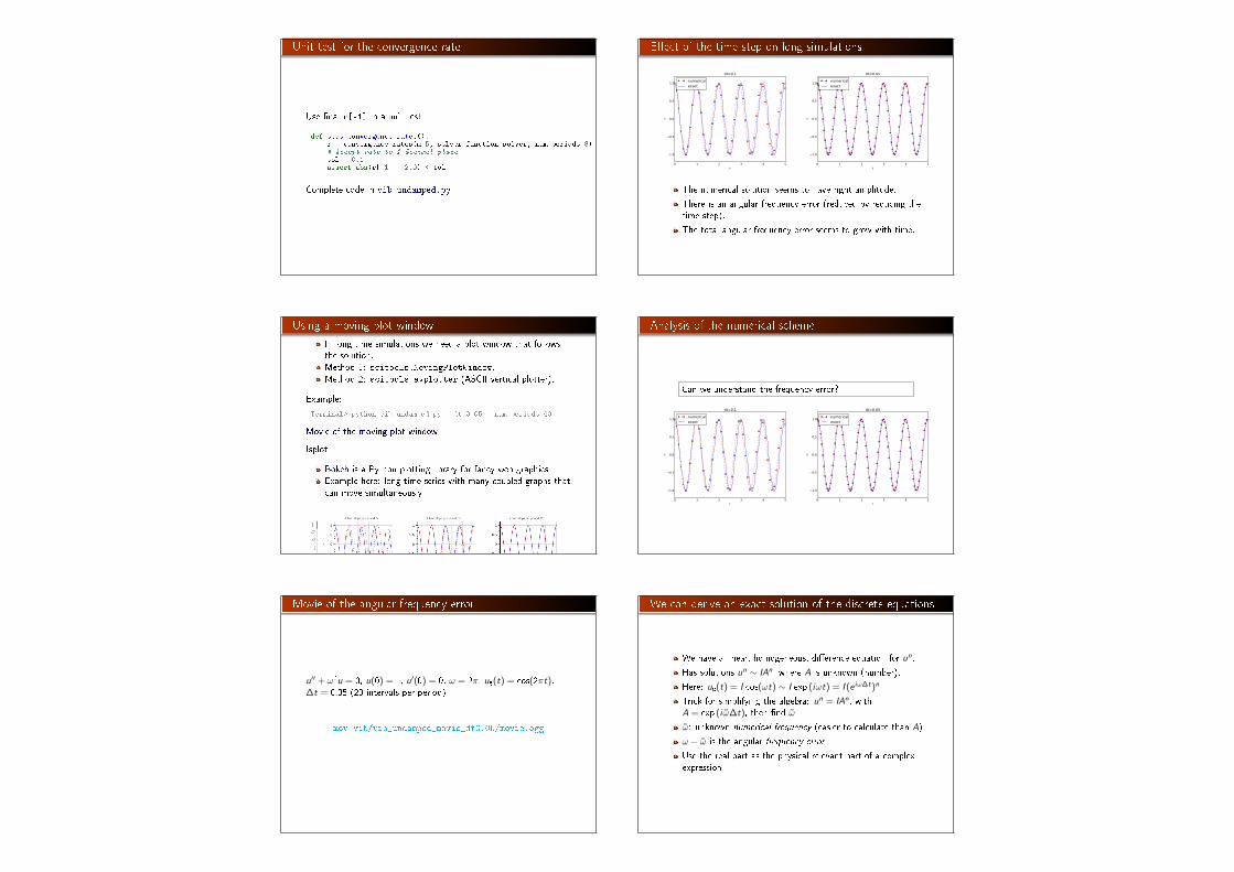
Unit test for the convergence rate

Use �nal r[-1] in a unit test:

def test_convergence_rates():r = convergence_rates(m=5, solver_function=solver, num_periods=8)# Accept rate to 1 decimal placetol = 0.1assert abs(r[-1] - 2.0) < tol

Complete code in vib_undamped.py.

E�ect of the time step on long simulations

0 1 2 3 4 5t

1.0

0.5

0.0

0.5

1.0

u

dt=0.1

numericalexact

0 1 2 3 4 5t

1.0

0.5

0.0

0.5

1.0

u

dt=0.05

numericalexact

The numerical solution seems to have right amplitude.

There is an angular frequency error (reduced by reducing thetime step).

The total angular frequency error seems to grow with time.

Using a moving plot window

In long time simulations we need a plot window that followsthe solution.Method 1: scitools.MovingPlotWindow.Method 2: scitools.avplotter (ASCII vertical plotter).

Example:

Terminal> python vib_undamped.py --dt 0.05 --num_periods 40

Movie of the moving plot window.

!splot

Bokeh is a Python plotting library for fancy web graphicsExample here: long time series with many coupled graphs thatcan move simultaneously

!splot

def bokeh_plot(u, t, legends, I, w, t_range, filename):"""Make plots for u vs t using the Bokeh library.u and t are lists (several experiments can be compared).legens contain legend strings for the various u,t pairs."""if not isinstance(u, (list,tuple)):

u = [u] # wrap in listif not isinstance(t, (list,tuple)):

t = [t] # wrap in listif not isinstance(legends, (list,tuple)):

legends = [legends] # wrap in list

import bokeh.plotting as pltplt.output_file(filename, mode='cdn', title='Comparison')# Assume that all t arrays have the same ranget_fine = np.linspace(0, t[0][-1], 1001) # fine mesh for u_etools = 'pan,wheel_zoom,box_zoom,reset,'\

'save,box_select,lasso_select'u_range = [-1.2*I, 1.2*I]font_size = '8pt'p = [] # list of plot objects# Make the first figurep_ = plt.figure(

width=300, plot_height=250, title=legends[0],x_axis_label='t', y_axis_label='u',x_range=t_range, y_range=u_range, tools=tools,title_text_font_size=font_size)

p_.xaxis.axis_label_text_font_size=font_sizep_.yaxis.axis_label_text_font_size=font_sizep_.line(t[0], u[0], line_color='blue')# Add exact solutionu_e = u_exact(t_fine, I, w)p_.line(t_fine, u_e, line_color='red', line_dash='4 4')p.append(p_)# Make the rest of the figures and attach their axes to# the first figure's axesfor i in range(1, len(t)):

p_ = plt.figure(width=300, plot_height=250, title=legends[i],x_axis_label='t', y_axis_label='u',x_range=p[0].x_range, y_range=p[0].y_range, tools=tools,title_text_font_size=font_size)

p_.xaxis.axis_label_text_font_size = font_sizep_.yaxis.axis_label_text_font_size = font_sizep_.line(t[i], u[i], line_color='blue')p_.line(t_fine, u_e, line_color='red', line_dash='4 4')p.append(p_)

# Arrange all plots in a grid with 3 plots per rowgrid = [[]]for i, p_ in enumerate(p):

grid[-1].append(p_)if (i+1) % 3 == 0:

# New rowgrid.append([])

plot = plt.gridplot(grid, toolbar_location='left')plt.save(plot)plt.show(plot)

Analysis of the numerical scheme

Can we understand the frequency error?

0 1 2 3 4 5t

1.0

0.5

0.0

0.5

1.0

u

dt=0.1

numericalexact

0 1 2 3 4 5t

1.0

0.5

0.0

0.5

1.0

u

dt=0.05

numericalexact

Movie of the angular frequency error

u′′ + ω2u = 0, u(0) = 1, u′(0) = 0, ω = 2π, ue(t) = cos(2πt),∆t = 0.05 (20 intervals per period)

mov-vib/vib_undamped_movie_dt0.05/movie.ogg

We can derive an exact solution of the discrete equations

We have a linear, homogeneous, di�erence equation for un.

Has solutions un ∼ IAn, where A is unknown (number).

Here: ue(t) = I cos(ωt) ∼ I exp (iωt) = I (e iω∆t)n

Trick for simplifying the algebra: un = IAn, withA = exp (i ω̃∆t), then �nd ω̃

ω̃: unknown numerical frequency (easier to calculate than A)

ω − ω̃ is the angular frequency error

Use the real part as the physical relevant part of a complexexpression

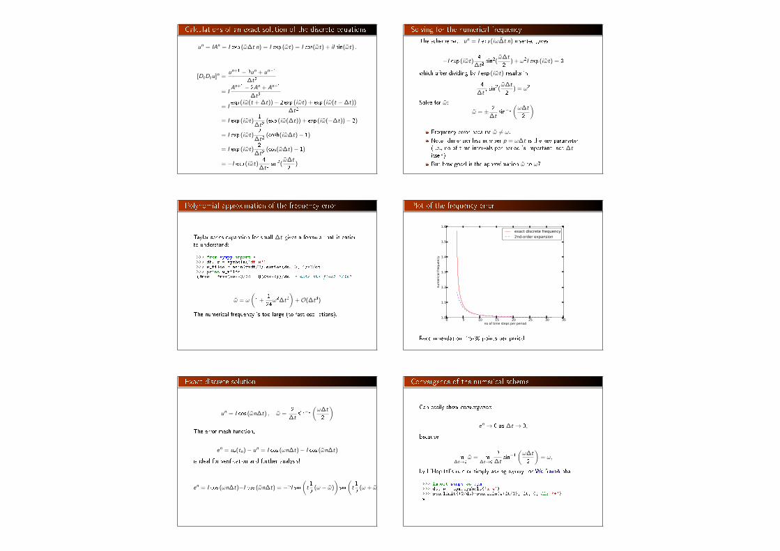
Calculations of an exact solution of the discrete equations

un = IAn = I exp (ω̃∆t n) = I exp (ω̃t) = I cos(ω̃t) + iI sin(ω̃t) .

[DtDtu]n =un+1 − 2un + un−1

∆t2

= IAn+1 − 2An + An−1

∆t2

= Iexp (i ω̃(t + ∆t))− 2 exp (i ω̃t) + exp (i ω̃(t −∆t))

∆t2

= I exp (i ω̃t)1

∆t2(exp (i ω̃(∆t)) + exp (i ω̃(−∆t))− 2)

= I exp (i ω̃t)2

∆t2(cosh(i ω̃∆t)− 1)

= I exp (i ω̃t)2

∆t2(cos(ω̃∆t)− 1)

= −I exp (i ω̃t)4

∆t2sin2(

ω̃∆t

2)

Solving for the numerical frequency

The scheme with un = I exp (iω∆̃t n) inserted gives

−I exp (i ω̃t)4

∆t2sin2(

ω̃∆t

2) + ω2I exp (i ω̃t) = 0

which after dividing by I exp (i ω̃t) results in

4

∆t2sin2(

ω̃∆t

2) = ω2

Solve for ω̃:

ω̃ = ± 2

∆tsin−1

(ω∆t

2

)

Frequency error because ω̃ 6= ω.

Note: dimensionless number p = ω∆t is the key parameter(i.e., no of time intervals per period is important, not ∆titself)

But how good is the approximation ω̃ to ω?

Polynomial approximation of the frequency error

Taylor series expansion for small ∆t gives a formula that is easierto understand:

>>> from sympy import *>>> dt, w = symbols('dt w')>>> w_tilde = asin(w*dt/2).series(dt, 0, 4)*2/dt>>> print w_tilde(dt*w + dt**3*w**3/24 + O(dt**4))/dt # note the final "/dt"

ω̃ = ω

(1 +

1

24ω2∆t2

)+O(∆t3)

The numerical frequency is too large (to fast oscillations).

Plot of the frequency error

0 5 10 15 20 25 30 35no of time steps per period

1.0

1.1

1.2

1.3

1.4

1.5

1.6

num

eric

al fr

eque

ncy

exact discrete frequency2nd-order expansion

Recommendation: 25-30 points per period.

Exact discrete solution

un = I cos (ω̃n∆t) , ω̃ =2

∆tsin−1

(ω∆t

2

)

The error mesh function,

en = ue(tn)− un = I cos (ωn∆t)− I cos (ω̃n∆t)

is ideal for veri�cation and further analysis!

en = I cos (ωn∆t)−I cos (ω̃n∆t) = −2I sin(t1

2(ω − ω̃)

)sin

(t1

2(ω + ω̃)

)

Convergence of the numerical scheme

Can easily show convergence:

en → 0 as ∆t → 0,

because

lim∆t→0

ω̃ = lim∆t→0

2

∆tsin−1

(ω∆t

2

)= ω,

by L'Hopital's rule or simply asking sympy: or WolframAlpha:

>>> import sympy as sym>>> dt, w = sym.symbols('x w')>>> sym.limit((2/dt)*sym.asin(w*dt/2), dt, 0, dir='+')w

Stability

Observations:

Numerical solution has constant amplitude (desired!), but anangular frequency error

Constant amplitude requires sin−1(ω∆t/2) to be real-valued⇒ |ω∆t/2| ≤ 1

sin−1(x) is complex if |x | > 1, and then ω̃ becomes complex

What is the consequence of complex ω̃?

Set ω̃ = ω̃r + i ω̃i

Since sin−1(x) has a *negative* imaginary part for x > 1,exp (iωt̃) = exp (−ω̃i t) exp (i ω̃r t) leads to exponential growthe−ω̃i t when −ω̃i t > 0

This is instability because the qualitative behavior is wrong

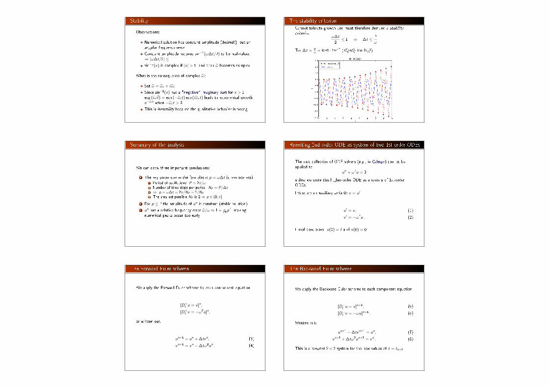
The stability criterion

Cannot tolerate growth and must therefore demand a stability

criterionω∆t

2≤ 1 ⇒ ∆t ≤ 2

ω

Try ∆t = 2ω + 9.01 · 10−5 (slightly too big!):

Summary of the analysis

We can draw three important conclusions:

1 The key parameter in the formulas is p = ω∆t (dimensionless)1 Period of oscillations: P = 2π/ω2 Number of time steps per period: NP = P/∆t3 ⇒ p = ω∆t = 2π/NP ∼ 1/NP

4 The smallest possible NP is 2 ⇒ p ∈ (0, π]

2 For p ≤ 2 the amplitude of un is constant (stable solution)

3 un has a relative frequency error ω̃/ω ≈ 1 + 124p

2, makingnumerical peaks occur too early

Rewriting 2nd-order ODE as system of two 1st-order ODEs

The vast collection of ODE solvers (e.g., in Odespy) cannot beapplied to

u′′ + ω2u = 0

unless we write this higher-order ODE as a system of 1st-orderODEs.

Introduce an auxiliary variable v = u′:

u′ = v , (1)

v ′ = −ω2u . (2)

Initial conditions: u(0) = I and v(0) = 0.

The Forward Euler scheme

We apply the Forward Euler scheme to each component equation:

[D+t u = v ]n,

[D+t v = −ω2u]n,

or written out,

un+1 = un + ∆tvn, (3)

vn+1 = vn −∆tω2un . (4)

The Backward Euler scheme

We apply the Backward Euler scheme to each component equation:

[D−t u = v ]n+1, (5)

[D−t v = −ωu]n+1 . (6)

Written out:

un+1 −∆tvn+1 = un, (7)

vn+1 + ∆tω2un+1 = vn . (8)

This is a coupled 2× 2 system for the new values at t = tn+1!

The Crank-Nicolson scheme

[Dtu = v t ]n+ 1

2 , (9)

[Dtv = −ωut ]n+ 1

2 . (10)

The result is also a coupled system:

un+1 − 1

2∆tvn+1 = un +

1

2∆tvn, (11)

vn+1 +1

2∆tω2un+1 = vn − 1

2∆tω2un . (12)

Comparison of schemes via Odespy

Can use Odespy to compare many methods for �rst-order schemes:

import odespyimport numpy as np

def f(u, t, w=1):u, v = u # u is array of length 2 holding our [u, v]return [v, -w**2*u]

def run_solvers_and_plot(solvers, timesteps_per_period=20,num_periods=1, I=1, w=2*np.pi):

P = 2*np.pi/w # duration of one perioddt = P/timesteps_per_periodNt = num_periods*timesteps_per_periodT = Nt*dtt_mesh = np.linspace(0, T, Nt+1)

legends = []for solver in solvers:

solver.set(f_kwargs={'w': w})solver.set_initial_condition([I, 0])u, t = solver.solve(t_mesh)

Forward and Backward Euler and Crank-Nicolson

solvers = [odespy.ForwardEuler(f),# Implicit methods must use Newton solver to convergeodespy.BackwardEuler(f, nonlinear_solver='Newton'),odespy.CrankNicolson(f, nonlinear_solver='Newton'),]

Two plot types:

u(t) vs t

Parameterized curve (u(t), v(t)) in phase space

Exact curve is an ellipse: (I cosωt,−ωI sinωt), closed andperiodic

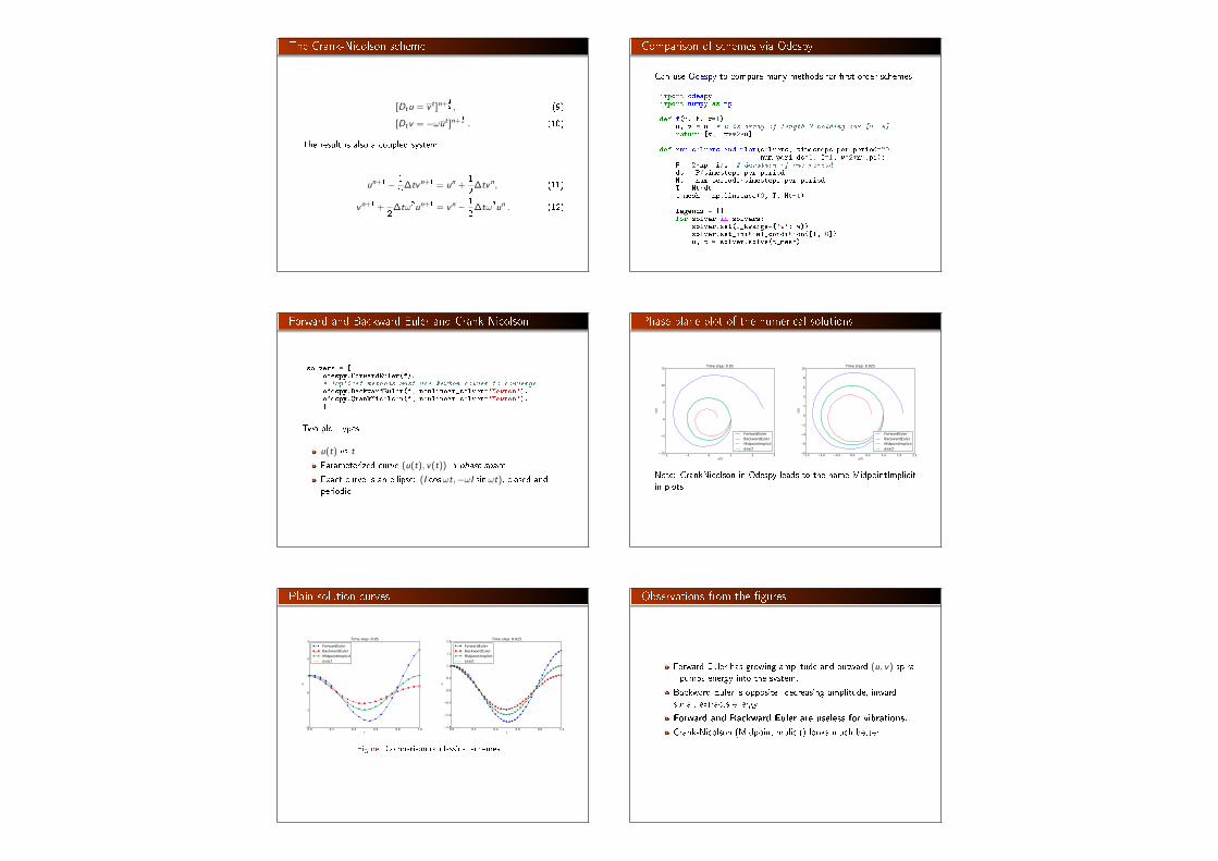
Phase plane plot of the numerical solutions

2 1 0 1 2 3u(t)

10

5

0

5

10

15

v(t

)

Time step: 0.05

ForwardEulerBackwardEulerMidpointImplicitexact

1.5 1.0 0.5 0.0 0.5 1.0 1.5 2.0u(t)

8

6

4

2

0

2

4

6

8

10

v(t

)

Time step: 0.025

ForwardEulerBackwardEulerMidpointImplicitexact

Note: CrankNicolson in Odespy leads to the name MidpointImplicitin plots.

Plain solution curves

0.0 0.2 0.4 0.6 0.8 1.0t

2

1

0

1

2

3

u

Time step: 0.05

ForwardEulerBackwardEulerMidpointImplicitexact

0.0 0.2 0.4 0.6 0.8 1.0t

1.5

1.0

0.5

0.0

0.5

1.0

1.5

2.0

u

Time step: 0.025

ForwardEulerBackwardEulerMidpointImplicitexact

Figure: Comparison of classical schemes.

Observations from the �gures

Forward Euler has growing amplitude and outward (u, v) spiral- pumps energy into the system.

Backward Euler is opposite: decreasing amplitude, inwardsprial, extracts energy.

Forward and Backward Euler are useless for vibrations.

Crank-Nicolson (MidpointImplicit) looks much better.

Runge-Kutta methods of order 2 and 4; short time series

1.5 1.0 0.5 0.0 0.5 1.0 1.5u(t)

8

6

4

2

0

2

4

6

8

v(t

)

Time step: 0.1

RK2RK4exact

1.5 1.0 0.5 0.0 0.5 1.0 1.5u(t)

8

6

4

2

0

2

4

6

8

v(t

)

Time step: 0.05

RK2RK4exact

0.0 0.2 0.4 0.6 0.8 1.0t

1.5

1.0

0.5

0.0

0.5

1.0

1.5

u

Time step: 0.1

RK2RK4exact

0.0 0.2 0.4 0.6 0.8 1.0t

1.5

1.0

0.5

0.0

0.5

1.0

1.5

u

Time step: 0.05

RK2RK4exact

Runge-Kutta methods of order 2 and 4; longer time series

8 6 4 2 0 2 4 6u(t)

50

40

30

20

10

0

10

20

30

40

v(t

)

Time step: 0.1

RK2RK4exact

1.5 1.0 0.5 0.0 0.5 1.0 1.5u(t)

8

6

4

2

0

2

4

6

8

v(t

)

Time step: 0.05

RK2RK4exact

0 2 4 6 8 10t

8

6

4

2

0

2

4

6

u

Time step: 0.1

RK2RK4exact

0 2 4 6 8 10t

1.5

1.0

0.5

0.0

0.5

1.0

1.5

u

Time step: 0.05

RK2RK4exact

Crank-Nicolson; longer time series

1.0 0.5 0.0 0.5 1.0u(t)

8

6

4

2

0

2

4

6

8

v(t

)

Time step: 0.1

MidpointImplicitexact

1.5 1.0 0.5 0.0 0.5 1.0 1.5u(t)

8

6

4

2

0

2

4

6

8

v(t

)

Time step: 0.05

MidpointImplicitexact

0 2 4 6 8 10t

1.0

0.5

0.0

0.5

1.0

u

Time step: 0.1

MidpointImplicitexact

0 2 4 6 8 10t

1.5

1.0

0.5

0.0

0.5

1.0

1.5

u

Time step: 0.05

MidpointImplicitexact

(MidpointImplicit means CrankNicolson in Odespy)

Observations of RK and CN methods

4th-order Runge-Kutta is very accurate, also for large ∆t.

2th-order Runge-Kutta is almost as bad as Forward andBackward Euler.

Crank-Nicolson is accurate, but the amplitude is not asaccurate as the di�erence scheme for u′′ + ω2u = 0.

Energy conservation property

The model

u′′ + ω2u = 0, u(0) = I , u′(0) = V ,

has the nice energy conservation property that

E (t) =1

2(u′)2 +

1

2ω2u2 = const .

This can be used to check solutions.

Derivation of the energy conservation property

Multiply u′′ + ω2u = 0 by u′ and integrate:

∫ T

0

u′′u′dt +

∫ T

0

ω2uu′dt = 0 .

Observing that

u′′u′ =d

dt

1

2(u′)2, uu′ =

d

dt

1

2u2,

we get

∫ T

0

(d

dt

1

2(u′)2 +

d

dt

1

2ω2u2)dt = E (T )− E (0),

where

E (t) =1

2(u′)2 +

1

2ω2u2

Remark about E (t)

E (t) does not measure energy, energy per mass unit.

Starting with an ODE coming directly from Newton's 2nd lawF = ma with a spring force F = −ku and ma = mu′′ (a:acceleration, u: displacement), we have

mu′′ + ku = 0

Integrating this equation gives a physical energy balance:

E (t) =1

2mv2

︸ ︷︷ ︸kinetic energy

+1

2ku2

︸ ︷︷ ︸potential energy

= E (0), v = u′

Note: the balance is not valid if we add other terms to the ODE.

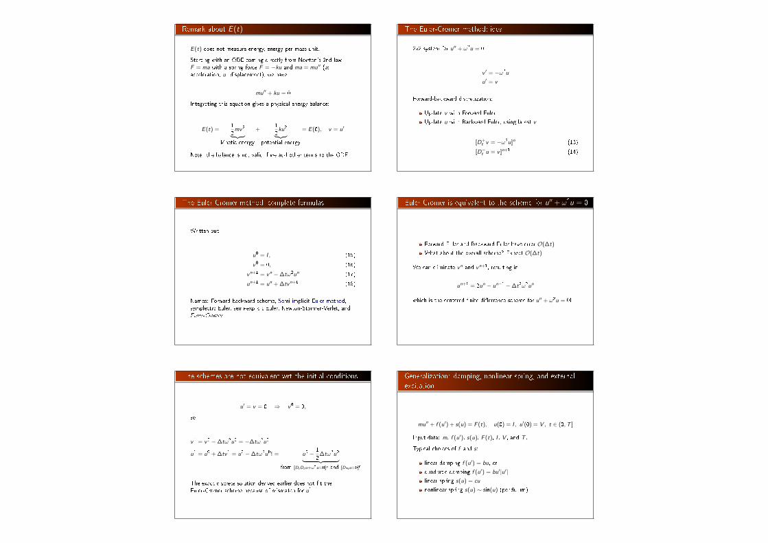
The Euler-Cromer method; idea

2x2 system for u′′ + ω2u = 0:

v ′ = −ω2u

u′ = v

Forward-backward discretization:

Update v with Forward Euler

Update u with Backward Euler, using latest v

[D+t v = −ω2u]n (13)

[D−t u = v ]n+1 (14)

The Euler-Cromer method; complete formulas

Written out:

u0 = I , (15)

v0 = 0, (16)

vn+1 = vn −∆tω2un (17)

un+1 = un + ∆tvn+1 (18)

Names: Forward-backward scheme, Semi-implicit Euler method,symplectic Euler, semi-explicit Euler, Newton-Stormer-Verlet, andEuler-Cromer.

Euler-Cromer is equivalent to the scheme for u′′ + ω2u = 0

Forward Euler and Backward Euler have error O(∆t)

What about the overall scheme? Expect O(∆t)...

We can eliminate vn and vn+1, resulting in

un+1 = 2un − un−1 −∆t2ω2un

which is the centered �nite di�errence scheme for u′′ + ω2u = 0!

The schemes are not equivalent wrt the initial conditions

u′ = v = 0 ⇒ v0 = 0,

so

v1 = v0 −∆tω2u0 = −∆tω2u0

u1 = u0 + ∆tv1 = u0 −∆tω2u0! = u0 − 1

2∆tω2u0

︸ ︷︷ ︸from [DtDtu+ω2u=0]n and [D2tu=0]0

The exact discrete solution derived earlier does not �t theEuler-Cromer scheme because of mismatch for u1.

Generalization: damping, nonlinear spring, and external

excitation

mu′′ + f (u′) + s(u) = F (t), u(0) = I , u′(0) = V , t ∈ (0,T ]

Input data: m, f (u′), s(u), F (t), I , V , and T .

Typical choices of f and s:

linear damping f (u′) = bu, or

quadratic damping f (u′) = bu′|u′|linear spring s(u) = cu

nonlinear spring s(u) ∼ sin(u) (pendulum)

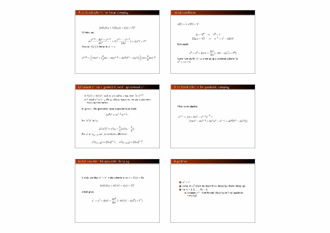
A centered scheme for linear damping

[mDtDtu + f (D2tu) + s(u) = F ]n

Written out

mun+1 − 2un + un−1

∆t2+ f (

un+1 − un−1

2∆t) + s(un) = F n

Assume f (u′) is linear in u′ = v :

un+1 =

(2mun + (

b

2∆t −m)un−1 + ∆t2(F n − s(un))

)(m+

b

2∆t)−1

Initial conditions

u(0) = I , u′(0) = V :

[u = I ]0 ⇒ u0 = I

[D2tu = V ]0 ⇒ u−1 = u1 − 2∆tV

End result:

u1 = u0 + ∆t V +∆t2

2m(−bV − s(u0) + F 0)

Same formula for u1 as when using a centered scheme foru′′ + ωu = 0.

Linearization via a geometric mean approximation

f (u′) = bu′|u′| leads to a quadratic equation for un+1

Instead of solving the quadratic equation, we use a geometricmean approximation

In general, the geometric mean approximation reads

(w2)n ≈ wn− 1

2wn+ 1

2 .

For |u′|u′ at tn:

[u′|u′|]n ≈ u′(tn +1

2)|u′(tn −

1

2)| .

For u′ at tn±1/2 we use centered di�erence:

u′(tn+1/2) ≈ [Dtu]n+ 1

2 , u′(tn−1/2) ≈ [Dtu]n−1

2

A centered scheme for quadratic damping

After some algebra:

un+1 =(m + b|un − un−1|

)−1×(2mun −mun−1 + bun|un − un−1|+ ∆t2(F n − s(un))

)

Initial condition for quadratic damping

Simply use that u′ = V in the scheme when t = 0 (n = 0):

[mDtDtu + bV |V |+ s(u) = F ]0

which gives

u1 = u0 + ∆tV +∆t2

2m

(−bV |V | − s(u0) + F 0

)

Algorithm

1 u0 = I

2 compute u1 (formula depends on linear/quadratic damping)3 for n = 1, 2, . . . ,Nt − 1:

1 compute un+1 from formula (depends on linear/quadraticdamping)

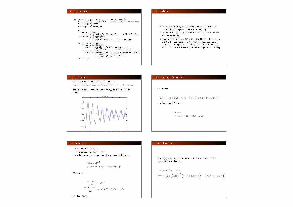
Implementation

def solver(I, V, m, b, s, F, dt, T, damping='linear'):dt = float(dt); b = float(b); m = float(m) # avoid integer div.Nt = int(round(T/dt))u = zeros(Nt+1)t = linspace(0, Nt*dt, Nt+1)

u[0] = Iif damping == 'linear':

u[1] = u[0] + dt*V + dt**2/(2*m)*(-b*V - s(u[0]) + F(t[0]))elif damping == 'quadratic':

u[1] = u[0] + dt*V + \dt**2/(2*m)*(-b*V*abs(V) - s(u[0]) + F(t[0]))

for n in range(1, Nt):if damping == 'linear':

u[n+1] = (2*m*u[n] + (b*dt/2 - m)*u[n-1] +dt**2*(F(t[n]) - s(u[n])))/(m + b*dt/2)

elif damping == 'quadratic':u[n+1] = (2*m*u[n] - m*u[n-1] + b*u[n]*abs(u[n] - u[n-1])

+ dt**2*(F(t[n]) - s(u[n])))/\(m + b*abs(u[n] - u[n-1]))

return u, t

Veri�cation

Constant solution ue = I (V = 0) ful�lls the ODE problemand the discrete equations. Ideal for debugging!

Linear solution ue = Vt + I ful�lls the ODE problem and thediscrete equations.

Quadratic solution ue = bt2 + Vt + I ful�lls the ODE problemand the discrete equations with linear damping, but not forquadratic damping. A special discrete source term can allowue to also ful�ll the discrete equations with quadratic damping.

Demo program

vib.py supports input via the command line:

Terminal> python vib.py --s 'sin(u)' --F '3*cos(4*t)' --c 0.03

This results in a moving window following the function on thescreen.

0 10 20 30 40 50 60t

1.0

0.5

0.0

0.5

1.0

u

dt=0.05

Euler-Cromer formulation

We rewrite

mu′′ + f (u′) + s(u) = F (t), u(0) = I , u′(0) = V , t ∈ (0,T ]

as a �rst-order ODE system

u′ = v

v ′ = m−1 (F (t)− f (v)− s(u))

Staggered grid

u is unknown at tn: un

v is unknown at tn+1/2: vn+ 1

2

All derivatives are approximated by centered di�erences

[Dtu = v ]n−1

2

[Dtv = m−1 (F (t)− f (v)− s(u))]n

Written out,

un − un−1

∆t= vn−

1

2

vn+ 1

2 − vn−1

2

∆t= m−1 (F n − f (vn)− s(un))

Problem: f (vn)

Linear damping

With f (v) = bv , we can use an arithmetic mean for bvn a laCrank-Nicolson schemes.

un = un−1 + ∆tvn−1

2 ,

vn+ 1

2 =

(1 +

b

2m∆t

)−1(vn−

1

2 + ∆tm−1(F n − 1

2f (vn−

1

2 )− s(un)

)).

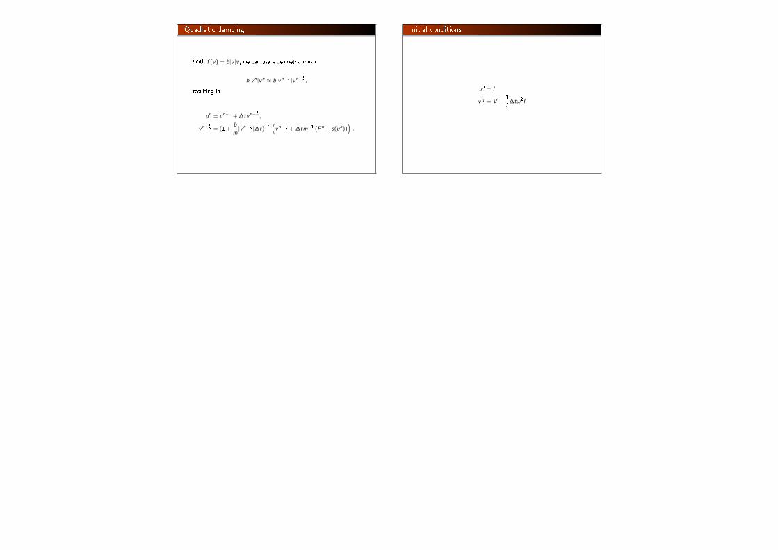
Quadratic damping

With f (v) = b|v |v , we can use a geometric mean

b|vn|vn ≈ b|vn− 1

2 |vn+ 1

2 ,

resulting in

un = un−1 + ∆tvn−1

2 ,

vn+ 1

2 = (1 +b

m|vn− 1

2 |∆t)−1(vn−

1

2 + ∆tm−1 (F n − s(un))).

Initial conditions

u0 = I

v1

2 = V − 1

2∆tω2I