A Simple Neural Network Approach to Software Cost Estimation · PDF fileA Simple Neural...

© 2013. Anupama Kaushik, A.K. Soni & Rachna Soni. This is a research/review paper, distributed under the terms of the Creative Commons Attribution-Noncommercial 3.0 Unported License http://creativecommons.org/licenses/by-nc/3.0/), permitting all non-commercial use, distribution, and reproduction inany medium, provided the original work is properly cited.

Global Journal of Computer Science and Technology Neural & Artificial Intelligence Volume 13 Issue 1 Version 1.0 Year 2013 Type: Double Blind Peer Reviewed International Research Journal Publisher: Global Journals Inc. (USA) Online ISSN: 0975-4172 & Print ISSN: 0975-4350

A Simple Neural Network Approach to Software Cost Estimation By Anupama Kaushik, A.K. Soni & Rachna Soni

Sharda University Greater Noida, India

Abstract - The effort invested in a software project is one of the most challenging task and most analyzed variables in recent years in the process of project management. Software cost estimation predicts the amount of effort and development time required to build a software system. It is one of the most critical tasks and it helps the software industries to effectively manage their software development process. There are a number of cost estimation models. Each of these models have their own pros and cons in estimating the development cost and effort. This paper investigates the use of Back-Propagation neural networks for software cost estimation. The model is designed in such a manner that accommodates the widely used COCOMO model and improves its performance. It deals effectively with imprecise and uncertain input and enhances the reliability of software cost estimates. The model is tested using three publicly available software development datasets. The test results from the trained neural network are compared with that of the COCOMO model. From the experimental results, it was concluded that using the proposed neural network model the accuracy of cost estimation can be improved and the estimated cost can be very close to the actual cost.

Keywords : artificial neural networks, back-propagation networks, COCOMO model, project management, soft computing techniques, software effort estimation.

GJCST-D Classification : B.2.m

A Simple Neural Network Approach to Software Cost Estimation

Strictly as per the compliance and regulations of:


Anupama Kaushik α, A.K. Soni σ & Rachna Soni ρ

Abstract - The effort invested in a software project is one of the most challenging task and most analyzed variables in recent years in the process of project management. Software cost estimation predicts the amount of effort and development time required to build a software system. It is one of the most critical tasks and it helps the software industries to effectively manage their software development process. There are a number of cost estimation models. Each of these models have their own pros and cons in estimating the development cost and effort. This paper investigates the use of Back-Propagation neural networks for software cost estimation. The model is designed in such a manner that accommodates the widely used COCOMO model and improves its performance. It deals effectively with imprecise and uncertain input and enhances the reliability of software cost estimates. The model is tested using three publicly available software development datasets. The test results from the trained neural network are compared with that of the COCOMO model. From the experimental results, it was concluded that using the proposed neural network model the accuracy of cost estimation can be improved and the estimated cost can be very close to the actual cost. Keywords : artificial neural networks, back-propagation networks, COCOMO model, project management, soft computing techniques, software effort estimation.

I. Introduction

oftware cost estimation is one of the most significant activities in software project management. It refers to the predictions of the

likely amount of effort, time and staffing levels required to build a software system. The effort prediction aspect of software is made at an early stage during project development, when the costing of the project is proposed for approval. It is concerned with the prediction of the person hour required to accomplish the task. However, estimates at the early stages of the development are the most difficult to obtain because very little is known about the project and the product at the beginning. So, estimating software development effort remains a complex problem and it continues to attract research attention. There are several cost estimation techniques proposed and they are grouped into two major categories: (1) Parametric models or Algorithmic models, which uses a mathematical formula Author α : Department of IT Maharaja Surajmal Institute of Tech. Delhi, India. E-mail : [email protected] Author σ : Department of IT Sharda University Greater Noida, India. Author ρ : Department of C.S. and Applications DAV College for Girls Yamuna Nagar, India.

to predict project cost based on the estimates of project size, the number of software engineers, and other process and product factors [1]. These models can be built by analysing the costs and attributes of completed projects and finding the closest fit formula to actual experience. (2) Non Parametric models or Non algorithmic models which are based on fuzzy logic (FL), artificial neural networks (ANN) and evolutionary computation (EC). In this paper, we focus on non parametric cost estimation models based on artificial neural networks, and particularly Back-Propagation networks. Neural networks have learning ability and are good at modelling complex nonlinear relationships. They also provide more flexibility to integrate expert knowledge into the model. There are many software cost estimation models that have been developed using neural networks over the years. The use of radial basis function neural networks for software effort estimation is well described by many researchers [2, 3 and 4]. The clustering algorithms used in those designs are the conventional algorithms.

K. Vinay Kumar et al. [5] Uses wavelet neural networks for predicting software development cost. B. Tirimula Rao et al. [6] provided a novel neural network approach for software cost estimation using functional link artificial neural network. G. Witting and G. Finnie [7] uses back propagation learning algorithms on a multilayer perceptron in order to predict development effort. N. Karunanitthi et al. [8] reports the use of neural networks for predicting software reliability including experiments with both feed forward and Jordan networks. N. Tadayon [9] also reports the use of neural network with a back propagation learning algorithm. However it was not clear how the dataset was divided for training and validation purposes. T.M. Khoshgoftaar et al.[10] presented a case study considering real time software to predict the testability of each module from source code static measures. Ch. Satyananda Reddy and KVSVN Raju [11] proposed a cost estimation model using multi layer feed forward neural network. Venkatachalam [12] also investigated the application of artificial neural network (ANN) to software cost estimation.

Artificial neural networks are the promising techniques to build predictive models. So, there is always a scope for developing effort estimation models with better predictive accuracy.

© 2013 Global Journals Inc. (US)

Globa

l Jo

urna

l of C

ompu

ter Sc

ienc

e an

d Te

chno

logy

V

olum

e XIII

Issu

e I V

ersio

n I

23

(DDDD DDDD

)Year

013

2D

S

II. Overview of the Models and Techniques sed

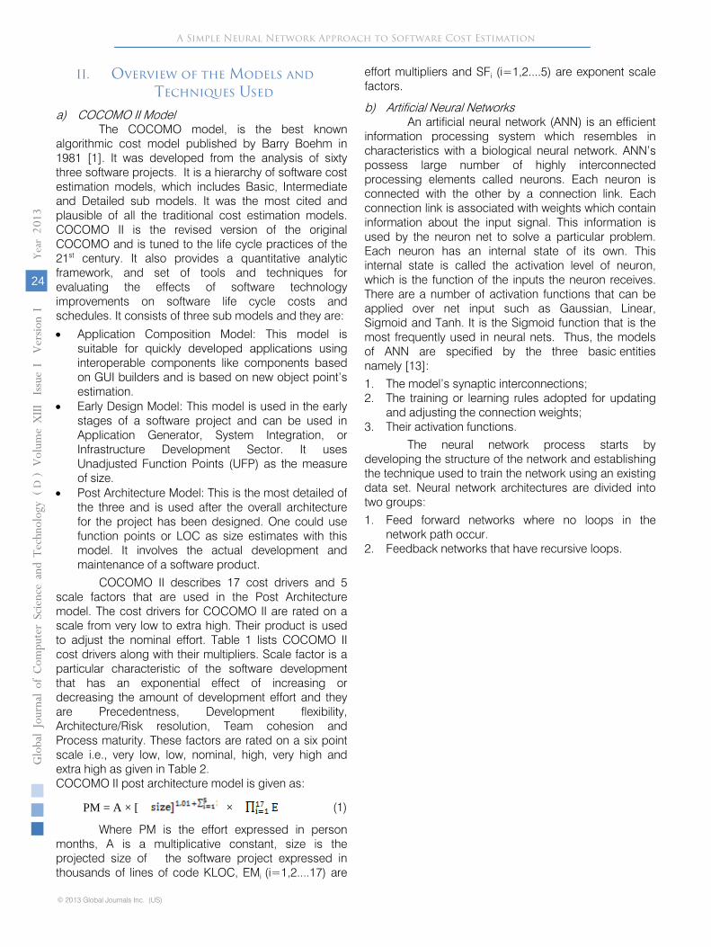
a) COCOMO II Model The COCOMO model, is the best known

algorithmic cost model published by Barry Boehm in 1981 [1]. It was developed from the analysis of sixty three software projects. It is a hierarchy of software cost estimation models, which includes Basic, Intermediate and Detailed sub models. It was the most cited and plausible of all the traditional cost estimation models. COCOMO II is the revised version of the original COCOMO and is tuned to the life cycle practices of the 21st century. It also provides a quantitative analytic framework, and set of tools and techniques for evaluating the effects of software technology improvements on software life cycle costs and schedules. It consists of three sub models and they are:

• Application Composition Model: This model is suitable for quickly developed applications using interoperable components like components based on GUI builders and is based on new object point’s estimation.

• Early Design Model: This model is used in the early stages of a software project and can be used in Application Generator, System Integration, or Infrastructure Development Sector. It uses Unadjusted Function Points (UFP) as the measure of size.

• Post Architecture Model: This is the most detailed of the three and is used after the overall architecture for the project has been designed. One could use function points or LOC as size estimates with this model. It involves the actual development and maintenance of a software product.

COCOMO II describes 17 cost drivers and 5 scale factors that are used in the Post Architecture model. The cost drivers for COCOMO II are rated on a scale from very low to extra high. Their product is used to adjust the nominal effort. Table 1 lists COCOMO II cost drivers along with their multipliers. Scale factor is a particular characteristic of the software development that has an exponential effect of increasing or decreasing the amount of development effort and they are Precedentness, Development flexibility, Architecture/Risk resolution, Team cohesion and Process maturity. These factors are rated on a six point scale i.e., very low, low, nominal, high, very high and extra high as given in Table 2. COCOMO II post architecture model is given as:

PM = A × [ × (1)

Where PM is the effort expressed in person months, A is a multiplicative constant, size is the projected size of the software project expressed in thousands of lines of code KLOC, EMi (i=1,2....17) are

effort multipliers and SFi (i=1,2....5) are exponent scale factors.

b) Artificial Neural Networks An artificial neural network (ANN) is an efficient

information processing system which resembles in characteristics with a biological neural network. ANN’s possess large number of highly interconnected processing elements called neurons. Each neuron is connected with the other by a connection link. Each connection link is associated with weights which contain information about the input signal. This information is used by the neuron net to solve a particular problem. Each neuron has an internal state of its own. This internal state is called the activation level of neuron, which is the function of the inputs the neuron receives. There are a number of activation functions that can be applied over net input such as Gaussian, Linear, Sigmoid and Tanh. It is the Sigmoid function that is the most frequently used in neural nets. Thus, the models of ANN are specified by the three basic entities namely [13]: 1. The model’s synaptic interconnections; 2. The training or learning rules adopted for updating

and adjusting the connection weights; 3. Their activation functions.

The neural network process starts by developing the structure of the network and establishing the technique used to train the network using an existing data set. Neural network architectures are divided into two groups: 1. Feed forward networks where no loops in the

network path occur. 2. Feedback networks that have recursive loops.


Globa

l Jo

urna

l of C

ompu

ter Sc

ienc

e an

d Te

chno

logy

V

olum

e XIII

Issu

e I V

ersio

n I

24

(DDDD

)


Year

013

2D

U

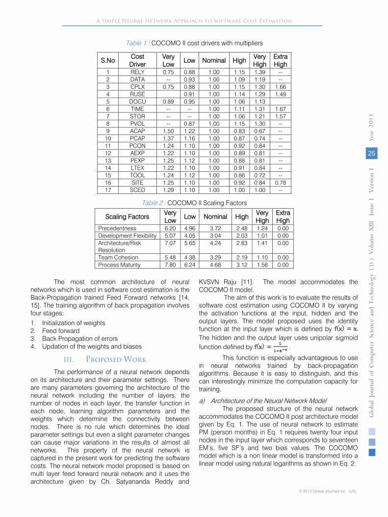
Table 1 : COCOMO II cost drivers with multipliers

Table 2 : COCOMO II Scaling Factors

The most common architecture of neural networks which is used in software cost estimation is the Back-Propagation trained Feed Forward networks [14, 15]. The training algorithm of back propagation involves four stages:

1.

Initialization of weights

2.

Feed forward

3.

Back Propagation of errors

4.

Updation of the weights and biases

III.

Proposed Work

The performance of a neural network depends on its architecture and their parameter settings. There are many parameters governing the architecture of the neural network including the number of layers, the number of nodes in each layer, the transfer function in each node, learning algorithm parameters and the weights which determine the connectivity between nodes. There is no rule which determines the ideal parameter settings but even a slight parameter changes can cause major variations in the results of almost

all

networks. This property of the neural network is captured in the present work for predicting the software costs. The neural network model proposed is based on multi layer feed forward neural network and it uses the architecture

given by

Ch. Satyananda Reddy and

KVSVN Raju [11]. The model accommodates the COCOMO II model.

The aim of this work is to evaluate the results of

software cost estimation using COCOMO II by varying the activation functions at the input, hidden and the output layers. The model proposed uses the identity function at the input layer which is defined by

The hidden and the output layer uses unipolar sigmoid function defined by

.

This function is especially advantageous to use in neural networks trained by back-propagation algorithms. Because it is easy to distinguish, and this can interestingly minimize the computation capacity for training.

a)

Architecture of the Neural Network Model

The proposed structure of the neural network accommodates the COCOMO II post architecture model given by Eq. 1. The use of neural network to estimate PM (person months) in Eq. 1 requires twenty four input nodes in the input layer which corresponds to seventeen EM’s, five SF’s and two bias values. The COCOMO model which is a non linear model is transformed into a linear model using natural logarithms as shown in Eq. 2.

S.No Cost Driver

Very Low

Low Nominal High Very High

Extra High

1 RELY 0.75 0.88 1.00 1.15 1.39 -- 2 DATA -- 0.93 1.00 1.09 1.19 -- 3 CPLX 0.75 0.88 1.00 1.15 1.30 1.66 4 RUSE 0.91 1.00 1.14 1.29 1.49 5 DOCU 0.89 0.95 1.00 1.06 1.13 6 TIME -- -- 1.00 1.11 1.31 1.67 7 STOR -- -- 1.00 1.06 1.21 1.57 8 PVOL -- 0.87 1.00 1.15 1.30 -- 9 ACAP 1.50 1.22 1.00 0.83 0.67 --

10 PCAP 1.37 1.16 1.00 0.87 0.74 -- 11 PCON 1.24 1.10 1.00 0.92 0.84 -- 12 AEXP 1.22 1.10 1.00 0.89 0.81 -- 13 PEXP 1.25 1.12 1.00 0.88 0.81 -- 14 LTEX 1.22 1.10 1.00 0.91 0.84 -- 15 TOOL 1.24 1.12 1.00 0.86 0.72 -- 16 SITE 1.25 1.10 1.00 0.92 0.84 0.78 17 SCED 1.29 1.10 1.00 1.00 1.00 --

Scaling Factors Very Low

Low Nominal High Very High

Extra High

Precedentness 6.20 4.96 3.72 2.48 1.24 0.00 Development Flexibility 5.07 4.05 3.04 2.03 1.01 0.00 Architecture/Risk Resolution

7.07 5.65 4.24 2.83 1.41 0.00

Team Cohesion 5.48 4.38 3.29 2.19 1.10 0.00 Process Maturity 7.80 6.24 4.68 3.12 1.56 0.00



Globa

l Jo

urna

l of C

ompu

ter Sc

ienc

e an

d Te

chno

logy

V

olum

e XIII

Issu

e I V

ersio

n I

25

(DDDD DDDD

)Year

013

2D

Ln (PM)=ln(A)+ln(EM1)+ln(EM2)+……+ln(EM17)+[1.01+SF1+……+SF5]*ln(size) (2)

The above equation becomes :

CPM = [b1+x1*z1+x2*z2+……+x17*z17]+ [b2+z18+……..+z22]*[yi+ln(size)] (3)

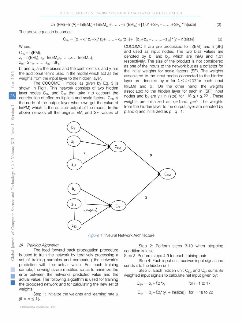
Where, CPM=ln(PM); z1=ln(EM1); z2=ln(EM2);……;z17=ln(EM17); z18=SF1;……..;z22=SF5; b1 and b2 are the biases and the coefficients xi and yi are the additional terms used in the model which act as the weights from the input layer to the hidden layer.

The COCOMO II model as given by Eq. 3 is shown in Fig.1. This network consists of two hidden layer nodes CEM and CSF that take into account the contribution of effort multipliers and scale factors. CPM is the node of the output layer where we get the value of ln(PM) which is the desired output of the model. In the above network all the original EMi and SFi values of

COCOMO II are pre processed to ln(EMi) and ln(SFi) and used as input nodes. The two bias values are denoted by b1 and b2, which are ln(A) and 1.01 respectively. The size of the product is not considered as one of the inputs to the network but as a cofactor for the initial weights for scale factors (SF). The weights associated to the input nodes connected to the hidden layer are denoted by xi for for each input ln(EMi) and b1. On the other hand, the weights associated to the hidden layer for each ln (SFi) input nodes and b2 are yi+ln (size) for . These weights are initialized as xi=1and yi=0. The weights from the hidden layer to the output layer are denoted by p and q and initialized as p=q=1.

Figure 1 : Neural Network Architecture

b) Training Algorithm The feed forward back propagation procedure

is used to train the network by iteratively processing a set of training samples and comparing the network’s prediction with the actual value. For each training sample, the weights are modified so as to minimize the error between the networks predicted value and the actual value. The following algorithm is used for training the proposed network and for calculating the new set of weights:

Step

2: Perform steps 3-10 when stopping condition is false.

Step 3: Perform steps 4-9 for each training pair.

Step 4: Each input unit receives input signal and sends it to the hidden unit.

Step

5: Each hidden unit CEM

and CSF sums its weighted input signals to calculate net input given by:

CEM

= b1+ zi*xi for i=1 to 17

CSF

= b2+ zi*(yi

+ ln(size)) for i=18 to 22

b1

z1

z17

b2

z18

z22

CEM

CSF

CPM

xi

yi+ln(size)

p

q


Globa

l Jo

urna

l of C

ompu

ter Sc

ienc

e an

d Te

chno

logy

V

olum

e XIII

Issu

e I V

ersio

n I

26

(DDDD

)


Year

013

2D

Step 1: Initialize the weights and learning rate α(

Apply sigmoidal activation function over CEM and CSF and send the output signal from the hidden unit to the input of output layer units.

Step 6: The output unit CPM, calculates the net input given by:

CPM =CEM*p+CSF*q

Apply sigmoidal activation function over CPM to compute the output signal Eest.

Step 7: Calculate the error correction term as: δ=Eact-Eest, where Eact is the actual effort from the dataset and Eest is the estimated effort from step 6. Step 8: Update the weights between hidden and the output layer as:

p(new)=p(old)+ α* δ* CEM

q(new)=q(old)+ α* δ* CSF

Step 9: Update the weights and bias between input and hidden layers as:

xi(new)=xi(old)+ α* δEM*zi for i=1 to 17 yi(new)=yi(old)+ α* δSF*zi for i=18 to 22 b1(new)=b1(old)+ α* δEM b2(new)=b2(old)+ α* δSF

The error is calculated as

δEM= δ*p; δSF= δ*q ;

Step 10: Check for the stopping condition. The stopping condition may be certain number of epochs reached or if the error is smaller than a specific tolerance.

Using this approach, we iterate forward and backward until the terminating condition is satisfied. The variable α used in the above formula is the learning rate, a constant, typically having a value between 0 and 1. The learning rate can be increased or decreased by the expert judgment indicating their opinion of the input effect. In other words the error should have more effect on the expert’s indication that a certain input had more contribution to the error propagation or vice versa. For each project, the expert estimator can identify the importance of the input value to the error in the estimation. If none selected by the expert, the changes in the weights are as specified by the learning algorithm. The network should also be trained according to correct inputs. For example, if during estimation ACAP (Analyst Capability) is set as high but after the end of the project, the management realizes that it was nominal or low, then the system should not consider this as a network error and before training the system, the better values of cost factors should be used to identify the estimated cost.

IV. Datasets and Evaluation Criteria

The data sets used in the present study comes from PROMISE Software Engineering Repository data

set [16] made publicly available for research purpose. The three datasets used are COCOMO 81 dataset, NASA 93 dataset and COCOMO_SDR.

The COCOMO 81 dataset consists of 63 projects which uses COCOMO model as described in section 2.1. Each project is described by its 17 cost drivers, 5 scale factors, the software size measured in KDSI (Kilo Delivered Source Instructions), the actual effort, total defects and the development time in months. The NASA 93 dataset consists of 93 NASA projects from different centres for various years. It consists of 26 attributes: 17 standard COCOMO-II cost drivers and 5 scale factors in the range Very_Low to Extra_High, lines of code measure (KLOC), the actual effort in person months, total defects and the development time in months.

The COCOMO_SDR dataset is from Turkish Software Industry. It consists of data from 12 projects and 5 different software companies in various domains. It has 24 attributes: 22 attributes from COCOMO II model, one being KLOC and the last being actual effort in man months.

The entire dataset is divided into two sets, training set and validation set in the ratio of 80:20 to get more accuracy of prediction. The proposed model is trained with the training data and tested with the test data.

The evaluation consists in comparing the accuracy of the estimated effort with the actual effort. A common criterion for the evaluation of cost estimation model is the Magnitude of Relative Error (MRE) and is defined as in Eq. 4.

MRE = (4)

The MRE values are calculated for each project in the validation set, while mean magnitude of relative error (MMRE) computes the average of MRE over N projects.

(5)

Another evaluation criterion is MdMRE, which measures the median of all MRE’s. MdMRE is less sensitive to extreme values. It exhibits a similar pattern to MMRE but it is more likely to select the true model if the underestimation is served.

Since MRE, MMRE and MdMRE are the most common evaluation criteria, they are adopted as the performance evaluators in the present paper.

V. Results and Discussion

This section presents and discusses the results obtained when applying the proposed neural network model to the COCOMO 81, NASA 93 and COCOMO_SDR datasets. The model is implemented in Matlab. The MRE, MMRE and MdMRE values are



Globa

l Jo

urna

l of C

ompu

ter Sc

ienc

e an

d Te

chno

logy

V

olum

e XIII

Issu

e I V

ersio

n I

27

(DDDD DDDD

)Year

013

2D

calculated for the projects in the validation set for all the three datasets. These values are then compared with the COCOMO model.

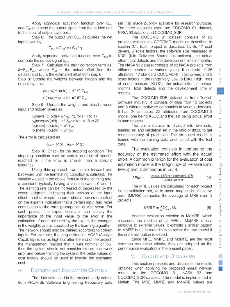
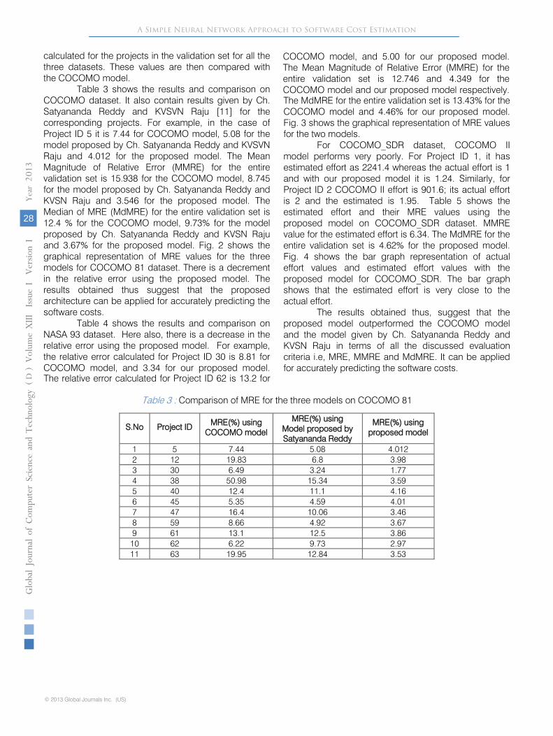
Table 3 shows the results and comparison on COCOMO dataset. It also contain results given by Ch. Satyananda Reddy and KVSVN Raju [11] for the corresponding projects. For example, in the case of Project ID 5 it is 7.44 for COCOMO model, 5.08 for the model proposed by Ch. Satyananda Reddy and KVSVN Raju and 4.012 for the proposed model. The Mean Magnitude of Relative Error (MMRE) for the entire validation set is 15.938 for the COCOMO model, 8.745 for the model proposed by Ch. Satyananda Reddy and KVSN Raju and 3.546 for the proposed model. The Median of MRE (MdMRE) for the entire validation set is 12.4 % for the COCOMO model, 9.73% for the model proposed by Ch. Satyananda Reddy and KVSN Raju and 3.67% for the proposed model. Fig. 2 shows the graphical representation of MRE values for the three models for COCOMO 81 dataset. There is a decrement in the relative error using the proposed model. The results obtained thus suggest that the proposed architecture can be applied for accurately predicting the software costs.

Table 4 shows the results and comparison on NASA 93 dataset. Here also, there is a decrease in the relative error using the proposed model. For example, the relative error calculated for Project ID 30 is 8.81 for COCOMO model, and 3.34 for our proposed model. The relative error calculated for Project ID 62 is 13.2 for

COCOMO model, and 5.00 for our proposed model. The Mean

Magnitude of Relative Error (MMRE) for the entire validation set is 12.746 and 4.349 for the COCOMO model and our proposed model

respectively. The MdMRE for the entire validation set is 13.43% for the COCOMO model and 4.46% for our proposed model. Fig. 3 shows the graphical representation of MRE values for the two models.

For COCOMO_SDR dataset, COCOMO II model performs very poorly. For Project ID 1, it has estimated effort as 2241.4 whereas the actual effort is 1 and with our proposed model it is 1.24. Similarly, for Project ID 2 COCOMO II effort is 901.6; its actual effort is 2 and the estimated is 1.95. Table 5 shows the estimated effort and their MRE values using the proposed model on COCOMO_SDR dataset. MMRE value for the estimated effort is 6.34. The

MdMRE for the entire validation set is 4.62% for the proposed model. Fig. 4 shows the bar graph representation of actual effort values and estimated effort values with the proposed model for COCOMO_SDR. The bar graph shows that the estimated effort is very close to the actual effort.

The results obtained thus, suggest that the proposed model outperformed the COCOMO model and the model given by Ch. Satyananda Reddy and KVSN

Raju in terms of all the discussed evaluation criteria i.e, MRE, MMRE and MdMRE. It can be applied for accurately predicting the software costs.

Table 3

:

Comparison of MRE for the three models on COCOMO 81

S.No

Project ID

MRE(%) using

COCOMO model

MRE(%) using

Model proposed by Satyananda Reddy

MRE(%) using proposed model

1

5

7.44

5.08

4.012

2

12

19.83

6.8

3.98

3

30

6.49

3.24

1.77

4

38

50.98

15.34

3.59

5

40

12.4

11.1

4.16

6

45

5.35

4.59

4.01

7

47

16.4

10.06

3.46

8

59

8.66

4.92

3.67

9

61

13.1

12.5

3.86

10

62

6.22

9.73

2.97

11

63

19.95

12.84

3.53


Globa

l Jo

urna

l of C

ompu

ter Sc

ienc

e an

d Te

chno

logy

V

olum

e XIII

Issu

e I V

ersio

n I

28

(DDDD

)


Year

013

2D

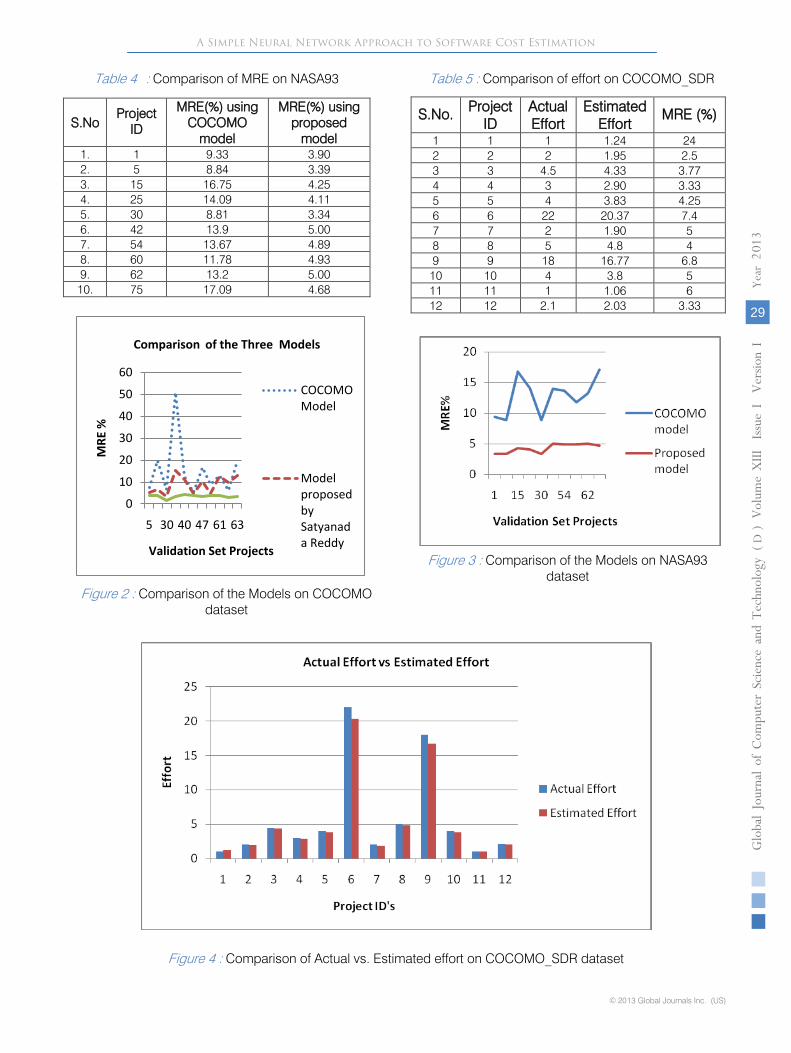
Table 4 : Comparison of MRE on NASA93 Table 5 : Comparison of effort on COCOMO_SDR

0

10

20

30

40

50

60

5 30 40 47 61 63

MRE

%

Validation Set Projects

Comparison of the Three Models

COCOMO Model

Model proposed by Satyanada Reddy

Figure 2 :

Comparison of the Models on COCOMO dataset

Figure 3 : Comparison of the Models on NASA93

dataset

Figure 4 : Comparison of Actual vs. Estimated effort on COCOMO_SDR dataset

S.No. Project ID

Actual Effort

Estimated Effort

MRE (%)

1 1 1 1.24 24 2 2 2 1.95 2.5 3 3 4.5 4.33 3.77 4 4 3 2.90 3.33 5 5 4 3.83 4.25 6 6 22 20.37 7.4 7 7 2 1.90 5 8 8 5 4.8 4 9 9 18 16.77 6.8

10 10 4 3.8 5 11 11 1 1.06 6 12 12 2.1 2.03 3.33

S.No Project

ID

MRE(%) using COCOMO

model

MRE(%) using proposed

model 1.

1

9.33

3.90 2.

5

8.84

3.39 3.

15

16.75

4.25 4.

25

14.09

4.11 5.

30

8.81

3.34 6.

42

13.9

5.00 7.

54

13.67

4.89 8.

60

11.78

4.93 9.

62

13.2

5.00 10.

75

17.09

4.68



Globa

l Jo

urna

l of C

ompu

ter Sc

ienc

e an

d Te

chno

logy

V

olum

e XIII

Issu

e I V

ersio

n I

29

(DDDD DDDD

)Year

013

2D

VI. Conclusion

Software development cost estimation is a challenging task for both the industrial as well as academic communities. The accurate predictions during the early stages of development of a software project can greatly benefit the development team. There are several effort estimation models that can be used in forecasting software development effort.

In the paper, Feed Forward Back Propagation model of neural network is used which maps the COCOMO model. The model used identity function at the input layer and sigmoidal function at the hidden and output layer. The model incorporates COCOMO dataset and COCOMO NASA 2 dataset to train and to test the network. Based on the experiments performed, it is observed that the proposed model outscored COCOMO model and the model proposed by Ch. Satyananda Reddy and KVSN Raju. Future research can replicate and confirm this estimation technique with other datasets for software cost estimation. Furthermore, the utilization of other neural networks architecture can also be applied for estimating software costs. This work can also be extended using Neuro Fuzzy approach.

References références referencias

1. Boehm, B.W., (1981) Software Engineering Economics, Prentice Hall, Englewood Cliffs, NJ.

2. Idri A.; Zakrani A.; Zahi A., (2010), Design of radial basis function neural networks for software effort estimation, IJCSI International Journal of Computer Science 7(4), 11-17.

3. Idri A.; Zahi A.; Mendes E.; Zakrani A., (2007), Software Cost Estimation Models using Radial Basis Function Neural Networks, International Conference on Software process and product measurements, 21-31.

4. Prasad Reddy P.V.G.D; Sudha K.R; Rama Sree P; Ramesh S.N.S.V.S.C, (2010) Software Effort Estimation using Radial Basis and Generalized Regression Neural Networks, Journal of computing 2(5), 87-92.

5. Vinay Kumar K.; Ravi V.; Mahil Carr; Raj Kiran N., (2008). Software development cost estimation using wavelet neural networks, The Journal of Systems and Software 81(11), 1853-1867.

6. Tirimula Rao B.; Sameet B.; Kiran Swathi G.; Vikram Gupta K.; Ravi Teja;Ch, Sumana S., (2009), A Novel Neural Network Approach for Software Cost Estimation using Functional Link Artificial Neural Network (FLANN), International Journal of Computer Science and Network Society 9(6), 126-131.

7. Witting G.; Finnie G.,(1994), Using Artificial Neural Networks and Function Points to estimate 4GL Software Development Effort, Journal of Information Systems,1(2), 87-94.

8. Karunanitthi N.; Whitely D.; and Malaiya Y.K., (1992), Using Neural Networks in Reliability Prediction. IEEE Software Engineering, 9(4), 53-59.

10. Khoshgoftaar T.M.; Allen E.B.; and Xu Z., (2000). Predicting testability of program modules using a neural network. Proceedings of 3rd IEEE Symposium on Application Specific Systems and Software Engineering Technology, 57-62.

11. Reddy C.S.; Raju KVSN, (2009). An Improved Fuzzy Approach for COCOMO’s Effort Estimation using Gaussian Membership Function. Journal of software 4(5), 452-459.

12. Venkatachalam A.R., (1993). Software Cost Estimation using artificial neural networks. Proceedings of the International Joint Conference on Neural Networks, 987-990.

13. Sivanandam S.N.; Deepa S.N., (2007). Principles of Soft Computing, Wiley, India.

14. Molokken K.; Jorgensen M., 2003. A review of software surveys on software effort estimation, Proceedings of IEEE International Symposium on Empirical Software Engineering ISESE, 223-230.

15. Huang S.; Chiu N., (2009). Applying fuzzy neural network to estimate software development effort, Proceedings of Applied Intelligence Journal 30(2), 73-83.

16. www.promisedata.org


Globa

l Jo

urna

l of C

ompu

ter Sc

ienc

e an

d Te

chno

logy

V

olum

e XIII

Issu

e I V

ersio

n I

30

(DDDD

)


Year

013

2D

9. Tadayon N., (2005). Neural Network Approach for Software Cost Estimation. Proceedings of the International Conference on Information Techno-logy: Coding and Computing (ITCC’05) 2(2), 815-818.

Global Journals Inc. (US)

Guidelines Handbook

www.GlobalJournals.org

A Simple Neural Network Approach to Software Cost Estimation · PDF fileA Simple Neural...

Documents

Transcript of A Simple Neural Network Approach to Software Cost Estimation · PDF fileA Simple Neural...