A SECOND-ORDER GRADIENT-LIKE DISSIPATIVE DYNAMICAL

SYSTEM with HESSIAN DRIVEN DAMPING.

Application to Optimization and Mechanics.

F. ALVAREZ ∗ H. ATTOUCH† J. BOLTE† P. REDONT †

Abstract

Given H a real Hilbert space and Φ : H → R a smooth C2 function, we study the dynamical system

(DIN) x(t) + αx(t) + β∇2Φ(x(t))x(t) +∇Φ(x(t)) = 0

where α and β are positive parameters. The inertial term x(t) acts as a singular perturbation and, in fact,regularization of the possibly degenerate classical Newton continuous dynamical system ∇2Φ(x(t))x(t)+∇Φ(x(t)) =0.

We show that (DIN) is a well-posed dynamical system. Due to their dissipative aspect, trajectories of (DIN)enjoy remarkable optimization properties. For example, when Φ is convex and argminΦ 6= ∅, then each trajectoryof (DIN) weakly converges to a minimizer of Φ. If Φ is real analytic, then each trajectory converges to a criticalpoint of Φ.

A remarkable feature of (DIN) is that one can produce an equivalent system which is first-order in time andwith no occurrence of the Hessian, namely

x(t) + c∇Φ(x(t)) + ax(t) + by(t) = 0y(t) + ax(t) + by(t) = 0

where a, b, c are parameters which can be explicitly expressed in terms of α and β. This allows to consider(DIN) when Φ is C1 only, or more generally, non-smooth or subject to constraints. This is first illustrated by agradient projection dynamical system exhibiting both viable trajectories, inertial aspects, optimization properties,and secondly by a mechanical system with impact.

Keywords: continuous Newton method, dissipative dynamical systems, asymptotic behaviour, gradient-like dy-namical systems, optimal control, second-order in time dynamical system, shocks in mechanics, gradient-projectionmethods.

AMS classification: 37Bxx, 37Cxx, 37Lxx, 37N40, 47H06.

1 Introduction

Let H be a real Hilbert space and Φ : H → R a smooth function whose gradient and Hessian are respectivelydenoted by ∇Φ and ∇2Φ. Our purpose is to study the following dynamical system

(DIN) x(t) + αx(t) + β∇2Φ(x(t))x(t) +∇Φ(x(t)) = 0,

where α and β are positive parameters. We use the following notations: t is the time variable, x ∈ H is the statevariable, trajectories in H are functions t 7→ x(t) whose first and second time derivatives are respectively denoted byx(t) and x(t).

∗Departamento de Ingenierıa Matematica, Centro de Modelamiento Matematico, Universidad de Chile, Blanco Encalada 2120, Santiago,Chile. Email: falvarez@dim.uchile.cl. Fax: (56-2) 688 3821. Partially supported by ECOS-CONICYT (C00E05), FONDAP in AppliedMathematics and FONDECYT 1990884.

†ACSIOM-CNRS FRE 2311, Departement de Mathematiques, case 51, Universite Montpellier II, Place Eugene Bataillon, 34095 Mont-pellier cedex 5, France

1

The above dynamical system will be referred to as the Dynamical Inertial Newton-like system, or (DIN) for short.This evolution problem comes naturally into play in various domains like optimization (minimization of Φ), mechanics(non-elastic shocks), control theory (asymptotic stabilization of oscillators) and PDE theory (damped wave equation).The terminology reflects the fact that (DIN) is a second order in time dynamical system, the acceleration x(t) beingassociated with inertial effects, while Newton’s dynamics refers to the action of the Hessian operator ∇2Φ(x(t)) onthe velocity vector x(t) (see (CN) below).

This paper focuses on the study of (DIN) as a dissipative dynamical system; accordingly, the investigation relies onLiapounov methods (for facts on dissipative systems see [17, 19, 35]). The convergence of the trajectories of (DIN), asthe time t goes to +∞, is established under various assumptions on Φ: Φ analytic (theorem 4.1), Φ convex (theorem5.1). Indeed, by following the trajectories of (DIN) as t goes to +∞, one expects to reach local minima of Φ (globalminima when Φ is convex), with clear applications to optimization and mechanics.

Let us discuss some motivations for the introduction of the (DIN) system.In recent years, numerous papers have been devoted to the study of dynamical systems that overcome some of the

drawbacks of the classical steepest descent method

(SD) x(t) +∇Φ(x(t)) = 0.

For instance, Alvarez and Perez study in [4] the Continuous Newton method

(CN) ∇2Φ(x(t))x(t) +∇Φ(x(t)) = 0

as a tool in optimization and show how to combine this dynamics with an approximation of Φ by smooth functionsΦε, when Φ is nonsmooth. On the other hand, Attouch, Goudou and Redont study in [11] the heavy ball with frictiondynamical system

(HBF) x(t) + αx(t) +∇Φ(x(t)) = 0,

where α > 0 can be interpreted as a viscous friction parameter. This dissipative dynamical system, which was firstintroduced by Polyak [31] and Antipin [6] enjoys remarkable optimization properties. For example, when Φ is convex,the trajectories of (HBF) weakly converge in H as t → +∞ to minimizers of Φ. This result, proved by Alvarez in[2], may be seen as an extension of the celebrated Bruck theorem for (SD) [16] to a second-order in time differentialdynamical system; see also [3] for an implicit discrete proximal version of their result.

There is a drastic difference between (SD) and (HBF). By contrast with (SD), (HBF) is no more a descent method:the function Φ(x(t)) does not decrease along the trajectories in general; it is the energy E(t) := 1

2 |x(t)|2 + Φ(x(t))that is decreasing. This confers to this system interesting properties for the exploration of local minima of Φ, see [11]for more details.

Both the Newton and the heavy ball with friction methods can be seen as second order extensions of (SD), thelatter in time (with x in addition to x) and the former in space (with ∇2Φ in addition to ∇Φ). Each one improves(SD) in some respects, but they also raise some new difficulties. In (CN), ∇2Φ(x(t)) may be degenerate and (CN) is nomore defined as a dynamical system, moreover ∇2Φ(x(t)) may be complicated to compute. In (HBF), the trajectoriesmay exhibit oscillations which are not desirable for a numerical optimization purpose.

If one combines the continuous Newton dynamical system with the heavy ball with friction system, the system soobtained,

(DIN) x + αx + β∇2Φ(x)x +∇Φ(x) = 0,

inherits most of the advantages of the two preceding systems and corrects both of the above-mentioned drawbacks: theterm ∇2Φ(x(t))x(t) is a clever geometric damping term, while the acceleration term x(t) makes (DIN) a well-poseddynamical system, even if ∇2Φ(x(t)) is degenerate; see Attouch and Redont [12] for a first study of this question.

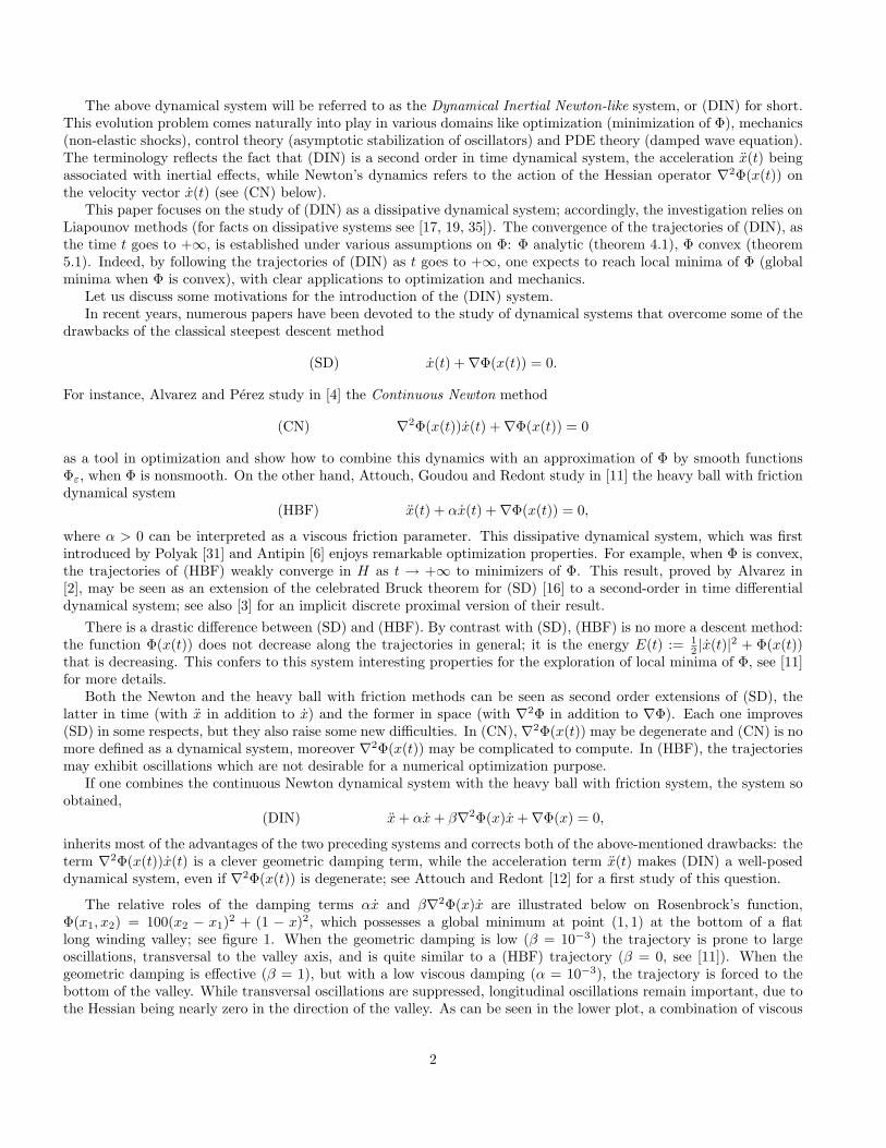
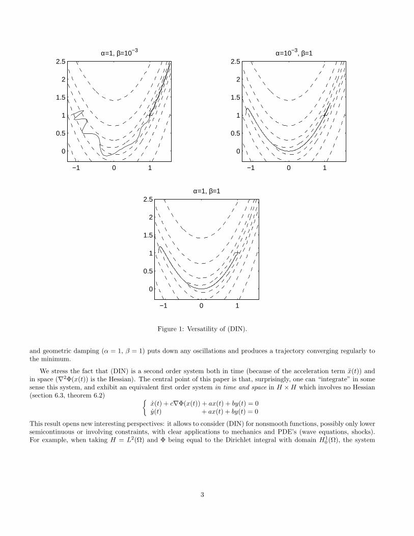
The relative roles of the damping terms αx and β∇2Φ(x)x are illustrated below on Rosenbrock’s function,Φ(x1, x2) = 100(x2 − x1)2 + (1 − x)2, which possesses a global minimum at point (1, 1) at the bottom of a flatlong winding valley; see figure 1. When the geometric damping is low (β = 10−3) the trajectory is prone to largeoscillations, transversal to the valley axis, and is quite similar to a (HBF) trajectory (β = 0, see [11]). When thegeometric damping is effective (β = 1), but with a low viscous damping (α = 10−3), the trajectory is forced to thebottom of the valley. While transversal oscillations are suppressed, longitudinal oscillations remain important, due tothe Hessian being nearly zero in the direction of the valley. As can be seen in the lower plot, a combination of viscous

2

−1 0 1

0

0.5

1

1.5

2

2.5α=1, β=10−3

−1 0 1

0

0.5

1

1.5

2

2.5α=10−3, β=1

−1 0 1

0

0.5

1

1.5

2

2.5α=1, β=1

Figure 1: Versatility of (DIN).

and geometric damping (α = 1, β = 1) puts down any oscillations and produces a trajectory converging regularly tothe minimum.

We stress the fact that (DIN) is a second order system both in time (because of the acceleration term x(t)) andin space (∇2Φ(x(t)) is the Hessian). The central point of this paper is that, surprisingly, one can “integrate” in somesense this system, and exhibit an equivalent first order system in time and space in H ×H which involves no Hessian(section 6.3, theorem 6.2)

x(t) + c∇Φ(x(t)) + ax(t) + by(t) = 0y(t) + ax(t) + by(t) = 0

This result opens new interesting perspectives: it allows to consider (DIN) for nonsmooth functions, possibly only lowersemicontinuous or involving constraints, with clear applications to mechanics and PDE’s (wave equations, shocks).For example, when taking H = L2(Ω) and Φ being equal to the Dirichlet integral with domain H1

0 (Ω), the system

3

(DIN) provides the following wave equation with higher order damping, which has been considered by Aassila in [1].

∂2u

∂t2+ α

∂u

∂t− β∆(

∂u

∂t)−∆u = 0 in Ω×]0, +∞[

u = 0 on ∂Ω×]0, +∞[

u(0) = u0,∂u

∂t(0) = u1 in Ω.

Another interesting situation corresponds to the case where Φ is proportional to the square of the distance functionto a convex set K: Φ(x) = ΨK,λ(x) = 1

2λdist2(x,K), λ > 0 (which is also the Moreau-Yosida approximation of theindicator function of K). In that case, (DIN), written under the form

xλ + 2ε√

λ∇2ΨK,λ(x)xλ +∇ΨK,λ(x) = −αxλ,

is closely related to a dynamical system introduced by Paoli and Schatzman [28] to model non-elastic shocks inmechanics.

Let us finally mention that the formulation of (DIN) as a first-order dynamical system which only involves thegradient of Φ, naturally suggests a way to define the second-order subdifferential ∂2Φ of non-smooth functions Φ. Itis certainly worthwile comparing this new aproach to ∂2Φ via dynamical systems, with the recent studies of R. T.Rockafellar [32], Mordukhovich-Outrata [26] and Kummer [22].

Clearly, a precise study of these quite involved questions is out of the scope of the present article. We just mentionthem in order to stress the importance and the versatility of the (DIN) system.

The paper is organized as follows. Section 2 gives the existence and the basic properties of the solution to (DIN).In section 3, we justify the terminology Dynamical Inertial Newton method by showing that (DIN) may be consideredas a perturbation of the continuous Newton method. The next two sections deal with the asymptotic behaviour of the(DIN) trajectories: convergence to a critical point is proved for an analytic function Φ (section 4), and convergence toa minimizer is proved for a convex function (section 5). Section 6 presents a first-order in time and space system thatis equivalent to (DIN). In section 7, constraints are introduced in that new system, which gives rise to a continuousgradient-projection system; the trajectories are shown to be viable and to enjoy optimizing properties. Section 8concludes the paper by an application to impact dynamics.

2 Global existence

Throughout this paper, H is a real Hilbert space with scalar product and norm denoted by 〈·, ·〉 and |·| respectively.Let Φ : H → R be a mapping satisfying:

(H)

Φ is bounded from below on HΦ is twice continuously differentiable on Hthe Hessian ∇2Φ is Lipschitz continuous on the bounded subsets of H.

Given two parameters α > 0 and β > 0 consider the following second order in time system in H

(DIN) x + αx + β∇2Φ(x)x +∇Φ(x) = 0.

Along every trajectory of (DIN), and for λ > 0 define

Eλ(t) = λΦ(x(t)) +12|x(t) + β∇Φ(x(t))|2. (1)

In particular, we will write for short

E(t) = Eαβ+1(t) = (αβ + 1)Φ(x(t)) +12|x(t) + β∇Φ(x(t))|2. (2)

Theorem 2.1 Let Φ satisfy (H). Then the following properties hold for (DIN), provided α > 0 and β > 0:

4

(i) For each (x0, x0) ∈ H × H, there exists a unique global solution x(t) of (DIN) satisfying the initial conditionsx(0) = x0 and x(0) = x0, with x ∈ C2([0,+∞[;H).

(ii) For every trajectory x(t) of (DIN) and λ ∈ [(1 − √αβ)2, (1 +√

αβ)2], the scalar function Eλ defined by (1) isbounded from below and decreasing on [0, +∞[, hence it converges as t → +∞. Moreover

• x and ∇Φ(x) belong to L2(0,+∞; H),

• limt→+∞ Φ(x(t)) exists,

• limt→+∞(x(t) + β∇Φx(t)) = 0.

(iii) Assuming moreover that x ∈ L∞(0, +∞; H), we have

• x, x, ∇Φ(x) and ∇2Φ(x) are bounded on [0, +∞[,

• limt→+∞∇Φ(x(t)) = limt→+∞ x(t) = limt→+∞ x(t) = 0.

Proof. (i) For any choice of initial conditions (x0, x0) ∈ H×H, the existence and uniqueness of a classic local solutionto (DIN) follow from the Cauchy-Lipschitz theorem applied to the equivalent first order in time system in the phasespace H ×H, Y = F (Y ), with

Y (t) =(

x(t)x(t)

)and F (u, v) =

(v

−αv − β∇2Φ(u)v −∇Φ(u)

).

Let x denote the maximal solution defined on some interval [0, Tmax[ with 0 < Tmax ≤ +∞. The regularity assumptionson Φ imply that x ∈ C2([0, Tmax[;H). Suppose, contrary to our claim, that Tmax < +∞. Differentiating E(t) (see(2)) and using (DIN), we successively obtain

E(t) = (αβ + 1)〈∇Φ(x(t)), x(t)〉+ 〈x(t) + β∇2Φ(x(t))x(t), x(t) + β∇Φ(x(t))〉= (αβ + 1)〈∇Φ(x(t)), x(t)〉 − 〈αx(t) +∇Φ(x(t)), x(t) + β∇Φ(x(t))〉= −α|x(t)|2 − β|∇Φ(x(t))|2. (3)

Hence E(t) is a Liapounov function for the trajectory x. Further, for all t ∈ [0, Tmax[

(αβ + 1)Φ(x(t)) +12|x(t) + β∇Φ(x(t))|2 + α

∫ t

0

|x(τ)|2dτ + β

∫ t

0

|∇Φ(x(τ))|2dτ = E(0). (4)

Since Φ is bounded from below and α, β > 0, we obtain that x and ∇Φ(x) belong to L2(0, Tmax; H). Therefore, forall 0 ≤ s ≤ t < Tmax

|x(t)− x(s)| ≤∫ t

s

|x(τ)|dτ ≤ √t− s

√∫ t

s

|x(τ)|2dτ ≤ √t− s ‖ x ‖L2(0,Tmax;H),

which shows that limt→Tmax x(t) exists. As a consequence, x is bounded on [0, Tmax[ and so is ∇2Φ(x) in view of theLipschitz continuity of ∇2Φ. Thus x = −αx + β∇2Φ(x)x − ∇Φ(x) belongs to L2(0, Tmax; H), and we have for all0 ≤ s ≤ t < Tmax

|x(t)− x(s)| ≤∫ t

s

|x(τ)|dτ ≤ √t− s ‖ x ‖L2(0,Tmax;H)

so that limt→Tmax x(t) exists. Applying the Cauchy-Lipschitz local existence theorem to (DIN) with initial data atTmax given by (limt→Tmax x(t), limt→Tmax x(t)), we can extend the maximal solution to an interval strictly larger than[0, Tmax[, which contradicts the maximality of the solution. Consequently, Tmax = +∞.

(ii) The point here is to realize that there is a whole family of Liapounov functions for the trajectory x. Indeed,setting for short (recall (1))

E±(t) = E1±√αβ = (1±√

αβ)2Φ(x(t)) +12|x(t) + β∇Φ(x(t))|2,

5

we obtainE±(t) = −|√αx(t)∓

√β∇Φ(x(t))|2.

Hence E+ and E− are two Liapounov functions for x, as well as any convex combination of them. As a result, for anyλ in [(1−√αβ)2, (1 +

√αβ)2], Eλ is decreasing on [0, +∞[, (e.g. E = Eαβ+1 = 1

2 (E+ + E−)). Further we have

(1±√

αβ)2Φ(x(t)) +12|x(t) + β∇Φ(x(t))|2 − E±(0) = −

∫ t

0

|√αx(τ)∓√

β∇Φ(x(τ))|2dτ.

Since Φ is bounded from below, we obtain that both |√αx−√β∇Φ(x)| and |√αx +√

β∇Φ(x)| belong to L2(0, +∞)and hence x and ∇Φ(x) are in L2(0, +∞;H). Now, since E+ and E− are decreasing and bounded from below,limt→+∞E+(t) and limt→+∞E−(t) exist. Therefore, Φ(x(t)) = 1

4√

αβ(E+(t)− E−(t)) admits a limit as t → +∞. As

a consequence, |x(t) + β∇Φ(x(t))| has a limit as t → +∞, which is zero because |x(t) + β∇Φ(x(t))| ∈ L2(0,+∞).

(iii) We now assume that x is in L∞(0, +∞; H). Then, by (H), ∇2Φ(x) and ∇Φ(x) are bounded on [0,+∞[; andso are x = (x + β∇Φ(x)) − β∇Φ(x) and x = −αx + β∇2Φ(x)x − ∇Φ(x). Set h(t) = 1

2 |∇Φ(x(t))|2 and note thath ∈ L1(0, +∞) and h = 〈∇2Φ(x)x,∇Φ(x)〉 ∈ L∞(0,+∞); then, by a standard argument, limt→+∞ h(t) = 0. Likewise,if we set k(t) = 1

2 |x(t)|2 then limt→+∞ k(t) = 0. It follows that x(t) → 0 as t → +∞.

Corollary 2.1 Assume that Φ : H → R satisfies (H) and is coercive, i.e. lim|x|→+∞ Φ(x) = +∞. Then the solutionx of (DIN) is in L∞(0,+∞; H). In particular, the properties in theorem 2.1(iii) hold.

Proof. It suffices to observe that (4) gives (αβ +1)Φ(x(t)) ≤ E(0). This estimate and the coerciveness of Φ imply thatthe trajectory x remains bounded.

3 (DIN) as a singular perturbation of Newton’s method

In this section we assume that Φ belongs to C2(H), with a Hessian Lipschitz continuous on bounded subsets, andthat Φ is coercive with ∇Φ strongly monotone on bounded subsets of H. More precisely, it is required that ∀R > 0,∃βR > 0 such that ∀x, y ∈ H

max|x|, |y| < R ⇒ 〈∇Φ(x)−∇Φ(y), x− y〉 ≥ βR|x− y|2. (5)

In particular, Φ is strictly convex and for all x ∈ H the Hessian operator ∇2Φ(x) is positive definite. Indeed, (5)yields ∀R > 0, ∃βR > 0: ∀x ∈ H, if |x| < R then ∀h ∈ H, 〈∇2Φ(x)h, h〉 ≥ βR|h|2. On the other hand, when H = Rn

and ∇2Φ(x) is positive definite for every x ∈ Rn, (5) holds with βR being a positive lower bound for the eigenvaluesof ∇2Φ(x) over the ball B(0, R).

For simplicity, take α = 0 and β = 1 and, for each ε > 0, consider a solution xε ∈ C2([0,∞[;H) to the initial valueproblem (xε does exist, see [12])

(ε-DIN)

εxε +∇2Φ(xε)xε +∇Φ(xε) = 0, t > 0,xε(0) = x0, xε(0) = x0,

where x0, x0 ∈ H are given. We are interested in the asymptotic behaviour of xε as ε → 0. Observe that (ε-DIN) maybe considered as a singular perturbation of the following evolution equation

(CN) ∇2Φ(x)x +∇Φ(x) = 0, t > 0,

x(0) = x0.

This is the Continuous Newton method for the minimization of Φ, which is a continuous version of the well-knownNewton iteration

∇2Φ(xk)(xk+1 − xk) +∇Φ(xk) = 0.

The unique solution x ∈ C2([0,∞[;H) of (CN) satisfies

d

dt[∇Φ(x(t))] = −∇Φ(x(t)),

6

which yields the following remarkable property of Newton’s trajectories

∇Φ(x(t)) = e−t∇Φ(x0). (6)

Moreover, since Φ is coercive, it follows from (5) and (6) that for an appropriate βR > 0, |x(t) − x| ≤ e−t

βR|∇Φ(x0)|,

where x is the unique minimizer of Φ. We refer the reader to [4, 13] for fuller treatments of the continuous Newtonmethod.

Proposition 3.1 There exists a constant C > 0 such that ∀t ≥ 0, |xε(t)−x(t)| ≤ C√

ε. Therefore, xε → x uniformlyon [0, +∞[.

Proof. Let us introduce the ε-energyUε(t) :=

ε

2|xε(t)|2 + Φ(xε(t)),

which satisfiesUε(t) = −〈∇2Φ(xε(t))xε(t), xε(t)〉 ≤ 0.

HenceUε(t) ≤ Uε(0) =

ε

2|x0|2 + Φ(x0), (7)

and consequently

sup0<ε≤1

supt≥0

Φ(xε(t)) ≤ 12|x0|2 + Φ(x0) =: α.

Since Φ is coercive, the sublevel set Γα(Φ) := x ∈ H : Φ(x) ≤ α is bounded and then sup0<ε≤1 supt≥0 |xε(t)| < R fora suitable constant R > 0. Similarly, we obtain that the solution x(t) of (CN) satisfies x(t) : t ≥ 0 ⊂ ΓΦ(x0)(Φ) ⊂Γα(Φ), so that we may assume that supt≥0 |x(t)| < R. By (5), we have

∀t > 0, |xε(t)− x(t)| ≤ 1βR|∇Φ(xε(t))−∇Φ(x(t))|. (8)

Notice that the differential equation in (ε-DIN) may be rewritten

d

dt[εxε(t) +∇Φ(xε(t))] +∇Φ(xε(t)) = 0.

Setting ωε(t) := εxε(t) +∇Φ(xε(t)), we obtain the nonhomogeneous initial value problem

ωε + ωε = εxε(t), t > 0,ωε(0) = εx0 +∇Φ(x0),

whose solution is given by

ωε(t) = e−t(εx0 +∇Φ(x0)) + ε

∫ t

0

e−(t−τ)xε(τ)dτ.

Thus

∇Φ(xε(t)) = e−t(εx0 +∇Φ(x0))− εxε(t) + ε

∫ t

0

e−(t−τ)xε(τ)dτ.

By (6) together with (8), we have

|xε(t)− x(t)| ≤ 1βR

(ε|x0|+ ε|xε(t)|+

∫ t

0

e−(t−τ)ε|xε(τ)|dτ

).

On the other hand, from the energy estimate (7), it follows that sup0<ε≤1 supt≥0 ε|xε(t)| ≤√

2ε(α− inf Φ). Conse-quently,

|xε(t)− x(t)| ≤ 1βR

(ε|x0|+ 2

√2ε(α− inf Φ)

)≤√

ε

βR

(|x0|+ 2

√2(α− inf Φ)

),

which completes the proof.

7

4 Convergence of the trajectories: Φ analytic

Since limt→+∞∇Φ(x(t)) = 0, it is natural to expect that for a sufficiently smooth Φ, trajectories will convergetowards a critical point of that function. Actually we show, in the finite-dimensional case, that if Φ is real analytic, xwill finally converge to x∞ ∈ H, with ∇Φ(x∞) = 0. The proof of this convergence result relies on an inequality dueto Lojasiewicz [25], linking Φ and ∇Φ in a neighbourhood of critical points. Lojasiewicz applied it in [24] to studythe asymptotic behaviour of a gradient-like system. More recently, Haraux and Jendoubi [20] showed that boundedtrajectories of HBF with an analytic potential converge towards critical points. This analyticity hypothesis is alsouseful for infinite dimensional systems with analytic nonlinearities, see Simon’s work [33] for the heat equation andHaraux [18] and Jendoubi [21] for the damped wave equation.

Let us recall the definition of a real analytic function.

Definition 4.1 Let Ω be an open subset of RN . A function Φ : Ω 7→ R is real analytic (in Ω), if for every pointξ = (ξ1, . . . , ξN ) in Ω there exist a neighbourhood U ⊆ Ω of ξ and real coefficients (cν1,...,νN

)(ν1,...,νN )∈NN such that

x = (x1, . . . , xN ) ∈ U ⇒ Φ(x) =∑

(ν1,...,νN )∈NN

cν1,...,νN(x1 − ξ1)ν1 . . . (xN − ξN )νN .

Lemma 4.1 (Lojasiewicz) Let Φ : RN → R be a function which is supposed to be analytic in a neighbourhood of acritical point a. Then, there exist σ > 0 and θ ∈]0, 1

2 [ such that 1

|x− a| < σ ⇒ |Φ(x)− Φ(a)|1−θ ≤ |∇Φ(x)|.

The next corollary extends the lemma to a compact connected set of critical points.

Corollary 4.1 Let Φ : Ω ⊆ RN → R be a function which is supposed to be analytic in the open set Ω. Let A be anonempty subset of Ω such that ∇Φ(a) = 0 for all a in A

1. If A is connected then Φ assumes a constant value on A, say ΦA.2. If A is connected and compact, then there exist σ > 0 and θ ∈]0, 1

2 [ such that

dist(x,A) < σ ⇒ |Φ(x)− ΦA|1−θ ≤ |∇Φ(x)|.

Proof. 1. Pick some a in A. After the lemma there exist σ > 0 and θ ∈]0, 12 [ such that

|x− a| < σ ⇒ |Φ(x)− Φ(a)|1−θ ≤ |∇Φ(x)|.

Hence if x belongs to A ∩ B(a, σ) where B(a, σ) is the open ball with center a and radius σ, then |Φ(x)− Φ(a)| = 0.As a consequence the set x ∈ A/Φ(x) = Φ(a) is open in A; as it is obviously closed in A and non-void it is equal toA.

2. Without restriction we may assume that Φ vanishes on A. According to Lojasiewicz’s lemma and owing to thecompactness of A, there exists a finite family (ai, σi, θi)i∈1,...,n with ai ∈ A, σi > 0, θi ∈]0, 1

2 [ such that- the balls B(ai, σi), build a finite open cover of A,- x ∈ Ω, |x− ai| < σi ⇒ |Φ(x)|1−θi ≤ |∇Φ(x)|.Resorting once more to the compactness of A, and to the continuity of Φ, we assert the existence of some σ > 0

such that

dist(x,A) < σ ⇒ x ∈ Ω, x ∈n⋃

i=1

B(ai, σi), |Φ(x)| ≤ 1.

If we set θ = min θi, then any x complying with dist(x, A) < σ verifies x ∈ Ω and x ∈ B(ai, σi) for some i ∈ 1, . . . , n;hence |Φ(x)|1−θ ≤ |Φ(x)|1−θi ≤ |∇Φ(x)|.

Theorem 4.1 Let x be a bounded solution of (DIN) and assume that Φ : RN 7→ R is analytic. Then x belongs toL1(0, +∞; H) and x(t) converges towards a critical point of Φ as t →∞.

1Originally ([25, p. 92]), the lemma states that θ lies in ]0, 1[; but it is harmless to suppose that σ satisfies |x−a| < σ ⇒ |Φ(x)−Φ(a)| ≤ 1,which, together with 0 < θ < 1, entails |Φ(x)− Φ(a)|1−θ/2 ≤ |Φ(x)− Φ(a)|1−θ; this justifies the assertion θ ∈]0, 1

2[.

8

Proof. Let ω(x) denote the ω-limit set of x. Classically ([19] e. g.), ω(x) is a compact connected set which consists ofcritical points of Φ. Moreover from theorem 2.1(ii) Φ assumes a constant value on ω(x), which we may suppose to be0. Further, dist(x(t), ω(x)) → 0 as t →∞.

After the corollary 4.1, there exist some T > 0 and some θ ∈]0, 12 [ such that

t ≥ T ⇒ |Φ(x(t))|1−θ ≤ |∇Φ(x(t))|. (9)

The proof of the convergence of x relies on the equality

− d

dtE(t)θ = −E(t)E(t)θ−1

and on lower bounds for −E(t) and E(t)θ−1 involving |x(t)|; recall that the energy E is defined by (2).First, we have (recall (3))

−E(t) ≥ 12

min(α, β)|x(t)|+ |∇Φ(x(t))|2. (10)

Further, for C = max(αβ + 1, β2), we have (recall (2))

E(t) ≤ C|Φ(x(t))|+ |x(t)|2 + |∇Φ(x(t))|2.Hence (using the inequality (r + s)1−θ ≤ r1−θ + s1−θ)

E(t)1−θ ≤ C1−θ|Φ(x(t))|1−θ + |x(t)|2(1−θ) + |∇Φ(x(t))|2(1−θ).Using (9), we have for t ≥ T

E(t)1−θ ≤ C1−θ|∇Φ(x(t))|+ |x(t)|2(1−θ) + |∇Φ(x(t))|2(1−θ).Since |∇Φ(x(t))| and |x(t)| tend to zero as t →∞ and since 2(1−θ) > 1, the quantities |∇Φ(x(t))|2(1−θ) and |x(t)|2(1−θ)

are negligible with respect to |∇Φ(x(t))| and |x(t)|. Therefore, there is some constant D > 0 such that for t ≥ T

E(t)1−θ ≤ D|∇Φ(x(t))|+ |x(t)|. (11)

If |∇Φ(x(t))|+ |x(t)| happens to vanish at some time t1 ≥ T , then owing to the unicity of the solution to (DIN), x(t)is equal to x(t1) for t ≥ t1, and the theorem is proved.

Else from (10) and (11) we obtain for t ≥ T

− d

dtE(t)θ ≥ 1

2Dmin(α, β)|∇Φ(x(t))|+ |x(t)|.

Since limt→∞E(t) exists, |x| belongs to L1([0, +∞[) and consequently limt→∞ x(t) exists.

5 Convergence of the trajectories: Φ convex

5.1 Weak convergence in the general convex case.

The proof of the asymptotic convergence in the convex case relies on the following lemma, which is essentially dueto Opial [27].

Lemma 5.1 (Opial) Let H be a Hilbert space and x : [0, +∞[ 7→ H a function such that there exists a nonempty setS ⊆ H verifying:

(a) if x(tn) x weakly in H for some tn → +∞ then x ∈ S,(b) ∀z ∈ S, limt→+∞ |x(t)− z| exists.

Then, x(t) weakly converges as t → +∞ to an element of S.

Theorem 5.1 Let Φ be a convex function satisfying (H) and assume that Argmin Φ 6= ∅. Let x be a solution of(DIN). Then for all z ∈ Argmin Φ, limt→+∞ |x(t)− z| exists, and x(t) weakly converges to a minimum point of Φ ast → +∞.

9

Proof. Write S = Argmin Φ and pick some z in S. In order to prove the existence of limt→+∞ |x(t)− z|, we introducean auxiliary energy

Eε(t) = E(t) + ε(α

2| x(t)− z |2 +〈x(t) + β∇Φ(x(t)), x(t)− z〉) (12)

where E is the energy defined by (2) and ε is a positive parameter. Let us show that, by choosing ε small enough, Eε

is a Liapounov function for (DIN). Thanks to (DIN) and (3), we have

Eε(t) = −(α− ε) | x(t) |2 −β | ∇Φ(x(t)) |2 −ε〈∇Φ(x(t)), x(t)− z〉+ ε〈β∇Φ(x(t)), x(t)〉.

Using the Young inequality for the last term, we obtain

Eε(t) ≤ −(α− 3ε

2) | x(t) |2 −β(1− εβ

2) | ∇Φ(x(t)) |2 −ε〈∇Φ(x(t)), x(t)− z〉. (13)

Take ε so small that each term in the previous expression is nonpositive (for the last term, use the fact that ∇Φ ismonotone and z ∈ S); then Eε is nonincreasing and we readily obtain

〈x(t) + β∇Φ(x(t)), x(t)− z〉+α

2| x(t)− z |2≤ 1

ε(Eε(0)− E(t)).

Since E(t) is bounded from below, because so is Φ, there exists some constant M such that

〈x(t) + β∇Φ(x(t)), x(t)− z〉+α

2| x(t)− z |2≤ M.

As x + β∇Φ(x) is bounded by theorem 2.1(ii), | x(t)− z | is bounded. Hence Eε(t), which is bounded from below anddecreasing, admits a limit as t → +∞. Moreover, theorem 2.1(ii-iii) asserts the following: limt→+∞E(t) exists andlimt→+∞ x(t) = limt→+∞∇Φ(x(t) = 0; hence, after (12), limt→+∞ |x(t)− z| exists.

In order to apply the Opial lemma we need to prove that the weak cluster points of the trajectory x are in S. Letx ∈ H and tn → +∞ be such that x(tn) x. Thanks to the convexity inequality, we have for any z ∈ S

Φ(z) = min Φ ≥ Φ(x(tn)) + 〈∇Φ(x(tn)), z − x(tn)〉.

Since ∇Φ(x(tn)) → 0 and Φ is lower semicontinuous, we obtain

minΦ ≥ lim infn→+∞

Φ(x(tn)) ≥ Φ(x),

which means that x ∈ S. The Opial lemma then applies, ensuring the weak convergence of x, and we also deduce thatΦ(x(t)) → minΦ as t →∞.

5.2 Strong convergence under int(Argmin Φ) 6= ∅.A counterexample due to Baillon [14] for the steepest descent equation x + ∇Φ(x) = 0 suggests that, likely,

convexity alone is not sufficient for the trajectories of (DIN) to converge strongly in H. Nevertheless, a result of Brezis[15, theorem 3.13] shows that the steepest descent trajectories do strongly converge under the additional hypothesisint(Argmin Φ) 6= ∅. This property also holds for (DIN) trajectories.

Proposition 5.1 Under the hypotheses of theorem 5.1, if moreover int(Argmin Φ) 6= ∅ then every trajectory of (DIN)converges to a minimizer of Φ with respect to the strong topology of H.

Proof. Fix z ∈ int(Argmin Φ) so that there exists ρ > 0 such that for every z′ ∈ H with |z′ − z| < ρ thenz′ ∈ int(Argmin Φ) and consequently ∇Φ(z′) = 0. By monotonicity of ∇Φ, we have

〈∇Φ(y), y − z〉 ≥ 〈∇Φ(y), z′ − z〉

for all y ∈ H and z′ ∈ H with ∇Φ(z′) = 0. Thus, for every y ∈ H

〈∇Φ(y), y − z〉 ≥ ρ|∇Φ(y)|.

10

Specialize y to x(t) to obtain for all t ≥ 0 and all z ∈ int(Argmin Φ)

〈∇Φ(x(t)), x(t)− z〉 ≥ ρ|∇Φ(x(t))|. (14)

Now, for ε > 0 small enough, the inequality (13) may be simplified to

0 ≤ ε〈∇Φ(x(t)), x(t)− z〉 ≤ −Eε(t);

integrating the latter yields

0 ≤ ε

∫ t

0

〈∇Φ(x(s)), x(s)− z〉ds ≤ Eε(0)− Eε(t).

Since limt→+∞Eε(t) exists, after the proof of theorem 5.1, we deduce that 〈∇Φ(x), x− z〉 belongs to L1(0, +∞), andso does |∇Φ(x)| in view of (14). If we now integrate (DIN)

x(t) + αx(t) + β∇Φ(x(t)) +∫ t

0

∇Φ(x(s))ds = x0 + αx0 + β∇Φ(x0),

we see that limt→+∞ x(t) exists in H, since limt→+∞ x(t) = limt→+∞∇Φ(x(t)) = 0, after theorem 2.1(iii).

5.3 Strong convergence under the symmetry property Φ(y) = Φ(−y).

Bruck [16] has shown that the convexity of Φ together with the symmetry assumption Φ(y) = Φ(−y) entailsthe strong convergence of the steepest descent trajectories. This result has been extended by Alvarez [2] to (HBF)trajectories and we extend it now to (DIN) trajectories.

Proposition 5.2 Under the hypotheses of Theorem 5.1, if moreover Φ is supposed to be even, i.e. ∀y ∈ H, Φ(y) =Φ(−y), then every trajectory of (DIN) converges to a minimizer of Φ with respect to the strong topology of H.

Proof. Let us successively consider the case αβ ≤ 1 and the case αβ > 1.

1. Case αβ ≤ 1. Fix t0 > 0 and define gt0 : [0, t0] 7→ R by

gt0(t) = |x(t)|2 − |x(t0)|2 − 12|x(t)− x(t0)|2.

We have gt0(t) = 〈x(t), x(t) + x(t0)〉 and gt0(t) = 〈x(t), x(t) + x(t0)〉+ |x(t)|2. From this we obtain

gt0(t) + αgt0(t) = 〈−β∇2Φ(x(t))x(t)−∇Φ(x(t)), x(t) + x(t0)〉+ |x(t)|2= d

dt 〈−β∇Φ(x(t)), x(t) + x(t0)〉+ 〈β∇Φ(x(t)), x(t)〉+ 1

β 〈−β∇Φ(x(t)), x(t) + x(t0)〉+ |x(t)|2= e−

1β t d

dte1β t〈−β∇Φ(x(t)), x(t) + x(t0)〉+ 〈x(t) + β∇Φ(x(t)), x(t)〉.

Set f(t) = 〈x(t) + β∇Φ(x(t)), x(t)〉. Since x and ∇Φ(x) are in L2(0,+∞; H), f belongs to L1(0, +∞). We have

d

dt[eαtgt0(t)] = e(α−1/β)t d

dte

1β t〈−β∇Φ(x(t)), x(t) + x(t0)〉+ eαtf(t)

and so, for every t ∈]0, t0]

eαtgt0(t)− gt0(0) =∫ t

0

e(α−1/β)τ d

ds[βes/βωt0(s)]s=τdτ +

∫ t

0

eατf(τ)dτ,

with ωt0(s) = 〈−∇Φ(x(s)), x(s) + x(t0)〉. An integration by parts yields

∫ t

0

e(α−1/β)τ d

ds[βes/βωt0(s)]s=τdτ = βeαtωt0(t)− βωt0(0) + (1− αβ)

∫ t

0

eατωt0(τ)dτ.

11

We conclude that

gt0(t) = 〈x0 + β∇Φ(x0), x0 + x(t0)〉e−αt + βωt0(t) +∫ t

0

e−α(t−τ)[(1− αβ)ωt0(τ) + f(τ)]dτ.

Set F (t) = 12 |x(t)|2+Φ(x(t)), which is nonincreasing because Φ is convex (in fact, F (t) = −α|x(t)|2−β〈∇2Φ(x(t))x(t), x(t)〉 ≤

0). Then, for all t ∈ [0, t0]

F (t) ≥ F (t0) =12|x(t0)|2 + Φ(x(t0)) =

12|x(t0)|2 + Φ(−x(t0)).

By convexity of ΦΦ(−x(t0)) ≥ Φ(x(t)) + 〈∇Φ(x(t)),−x(t0)− x(t)〉

and consequently

ωt0(t) = 〈−∇Φ(x(t)), x(t) + x(t0)〉 ≤ 12|x(t)|2.

Therefore

gt0(t) ≤ 〈x0 + β∇Φ(x0), x0 + x(t0)〉e−αt +β

2|x(t)|2 +

∫ t

0

e−α(t−τ)h(τ)dτ,

where h(t) = 1−αβ2 |x(t)|2 + |f(t)| ∈ L1(0,∞). Hence, for all t ∈ [0, t0]

gt0(t0)− gt0(t) ≤1α〈x0 + β∇Φ(x0), x0 + x(t0)〉(e−αt − e−αt0) +

β

2

∫ t0

t

|x(τ)|2dτ +∫ t0

t

∫ θ

0

e−α(θ−τ)h(τ)dτdθ

which gives

12|x(t0)− x(t)|2 ≤ |x(t)|2 − |x(t0)|2 +

1α〈x0 + β∇Φ(x0), x0 + x(t0)〉(e−αt − e−αt0) +

∫ t0

t

p(θ)dθ,

where p ∈ L1(0,∞). We know that x(t) x∞ as t → ∞ where x∞ ∈ ArgminΦ. Moreover, for all z ∈ ArgminΦthere exists some lz ∈ R such that |x(t)− z|2 → lz, as t →∞ (see theorem 5.1). Since Φ is even, 0 is a minimizer of Φso that there is some l0 ∈ R such that limt→∞ |x(t)|2 = l0. From the inequality above it follows that x(t) : t → ∞is a Cauchy net in H, hence x(t) → x∞ strongly in H.

2. Case αβ > 1. The conclusion follows in this case from a well-known result of Bruck [16] applied to an equivalentgradient-type first order system defined on H ×H (see section 6.3).

Remark. If Φ(x) = 12 〈Ax, x〉 where A : H 7→ H is a positive self-adjoint and bounded linear operator, then

ArgminΦ = KerA = z ∈ H : Az = 0 and x(t) strongly converges in H to the projection of x0 + 1α x0 on KerA.

Indeed, for every z ∈ KerA and t > 0 we have

〈x(t) + αx(t)− x0 − αx0, z〉 =∫ t

0〈−β∇2Φ(x(τ))x(τ)−∇Φ(x(τ)), z〉dτ

=∫ t

0〈−βAx(τ)−Ax(τ), z〉dτ

=∫ t

0〈−βx(τ)− x(τ), Az〉dτ = 0.

Since x(t) → 0 and x(t) → x∞ ∈ KerA strongly, we deduce that 〈x∞ − x0 − 1α x0, z〉 = 0 for all z ∈ KerA, which

proves our claim.

6 (DIN) as a first order in time gradient-like system

This part is devoted to establishing two remarkable properties of (DIN):- actually (DIN) proves to be equivalent to a system of first order in time with no occurrence of the Hessian of Φ,- further, if the positive parameters α and β satisfy αβ > 1, then (DIN) is a gradient system.

12

6.1 (DIN) as a system of first order in time and with no occurrence of the Hessian ofΦ

In this section, the requirements on the constants α, β and on the function Φ in (DIN) may be relaxed to β 6= 0and Φ ∈ C2(H) only.

Let x be a solution of (DIN), and define the function y by

x + β∇Φ(x) + (α− 1β

)x +1β

y = 0. (15)

Differentiate (15) to obtain

β[x + β∇2Φ(x)x + (α− 1β

)x] + y = 0,

which, in view of (DIN), yields

β[−∇Φ(x)− 1β

x] + y = 0. (16)

Adding (15) and (16) gives

(α− 1β

)x + y +1β

y = 0. (17)

Collecting (15) and (17) gives the first-order system

x + β∇Φ(x) +(α− 1β

)x +1β

y = 0

y +(α− 1β

)x +1β

y = 0(18)

Conversely, let (x, y) be a solution of (18). Combining the two lines of (18) yields

y = x + β∇Φ(x)

while differentiating the first equation yields

x + β∇2Φ(x)x + (α− 1β

)x +1β

y = 0.

Substituting the value of y in the above equation gives (DIN) again. Thus (DIN) is equivalent to (18).It is natural now to introduce the following first-order sytem (where g stands for generalized)

(g-DIN)

x + β∇Φ(x) +ax + by = 0y +ax + by = 0

which is a slight generalization of (18); indeed (g-DIN) is (18) if we set

a = α− 1β

, b =1β

(19)

The following theorem summarizes the above computation, and emphasizes the equivalence of (DIN), which is of secondorder in time and involves the Hessian of Φ, with a system which is of first order in time and with no occurrence ofthe Hessian.

Theorem 6.1 Suppose Φ ∈ C2(H), and let the constants α, β, a, b satisfy β 6= 0 and (19). The systems (DIN) and(g-DIN) are equivalent in the sense that x is a solution of (DIN) if and only if there exists y ∈ C2([0,+∞[,H) suchthat (x, y) is a solution of (g-DIN).

13

6.2 Existence and asymptotic behaviour of the solutions of (g-DIN)

Beyond being of first order in time, the system (g-DIN) is interesting because it does not involve the Hessian ofΦ. As a first consequence, the numerical solution of (DIN) is highly simplified, since it may be performed on (g-DIN)and only requires approximating the gradient of Φ. As a second consequence, (g-DIN) allows to give a sense to (DIN)when Φ is of class C1 only, or when Φ is nonsmooth or involves constraints, provided that a notion of generalizedgradient is available (e.g. the subdifferential set for a convex function Φ). But that remark would be of little utilityif (g-DIN) did not have good existence and convergence properties under the sole assumption Φ ∈ C1(H); recall that(DIN), as studied in the previous sections, requires Φ ∈ C2(H). Actually (g-DIN) enjoys the same properties as (DIN)does, at least if Φ ∈ C1,1(H), and theorems similar to theorems 2.1 and 5.1 can be stated about (g-DIN).

Theorem 6.2 Assume that Φ : H 7→ R is bounded from below, differentiable with ∇Φ Lipschitz continuous on thebounded subsets of H; assume further β > 0, b > 0, b + a > 0 in (g-DIN). Then the following properties hold:

(i) For each (x0, y0) in H×H, there exists a unique solution (x, y) of (g-DIN) defined on the whole interval [0, +∞[,which belongs to C1(0,∞; H)× C2(0,∞;H) and satisfies the initial conditions x(0) = x0 and y(0) = y0.

(ii) For any λ ∈ [β(√

a + b −√

b)2, β(√

a + b +√

b)2] the function Fλ : (x, y) ∈ H × H 7→ λΦ(x) + 12 |ax + by|2 is

a Liapounov function of (g-DIN); for every solution (x, y) the energy Fλ(x(t), y(t)) is decreasing on [0, +∞[,bounded from below and hence it converges to some real value as t → +∞. Moreover

• x and ∇Φ(x) belong to L2(0,+∞; H),

• limt→+∞ Φ(x(t)) exists,

• limt→+∞(x(t) + β∇Φx(t)) = 0.

(iii) Assuming moreover that x is in L∞(0, +∞; H), then we have

• x, ∇Φ(x) are bounded on [0, +∞[,

• limt→+∞∇Φ(x(t)) = limt→+∞ x(t) = 0.

Theorem 6.3 In addition to the hypotheses of theorem 6.2, assume that Φ is convex, and that ArgminΦ, the set ofminimizers of Φ on H, is nonempty. Then for any solution (x, y)) of (g-DIN), x(t) weakly converges to a minimizerof Φ on H as t goes to infinity.

The proof follows the lines of theorems 2.1 and 5.1 and will not be given. Besides, a more general situation will beexaminated in section 7 (cf. theorems 7.1 and 7.2).

Theorem 2.1 is a mere corollary of theorems 6.1 and 6.2. Indeed suppose that Φ and α, β meet the assumptionsof theorem 2.1: Φ satisfies (H) and α > 0, β > 0. Then ∇Φ is Lipschitz continuous on the bounded subsets of H, andthe constants a = α − 1/β and b = 1/β satisfy a + b > 0, b > 0. So the assumptions of theorem 6.2 are met; in viewof the equivalence between (DIN) and (g-DIN) given by theorem 6.1, the conclusions of theorem 6.2 apply to (DIN).

Further if Φ ∈ C2(H) meets the assumptions of theorem 6.2, the system (DIN) makes sense but theorem 2.1 doesnot apply since ∇2Φ need not be Lipschitz continuous. Yet we can resort to theorems 6.1 and 6.2 to assert the existenceof a solution to (DIN) enjoying the properties stated in theorem 6.2. Consequently the assumptions of theorem 2.1may be weakened, while its conclusions remain valid, as far as x and ∇2Φ, which need not exist in a classical sense,are not concerned.

Likewise theorem 5.1 is a corollary of theorems 6.1 and 6.3 and its hypotheses may be weakened.

6.3 (DIN) as a gradient system if αβ > 1

Suppose Φ ∈ C1(H) and a > 0, b > 0 in (g-DIN). Rescaling the variable y by y =√

ab z transforms (g-DIN) into

the equivalent system x + β∇Φ(x) +ax +

√abz = 0

z +√

abx + bz = 0(20)

We note that (20) is exactly the gradient system

X +∇E(X) = 0 (21)

14

where X = (x, z) and E : H ×H 7→ R is defined by

E(X) = βΦ(x) +12|√ax +

√bz|2.

Suppose now that Φ belongs to C2(H) and let us turn to (DIN) which we know is equivalent to (g-DIN) witha = α − 1/β, b = 1/β. If α, β satisfy αβ > 1 in addition to α > 0, β > 0, then a, b satisfy a > 0, b > 0. As aconsequence (DIN) is equivalent to the gradient system (20); using the parameters α, β the expression of E is

E(X) = E(x, z) = βΦ(x) +12β|√

αβ − 1x + z|2 (22)

We state as a proposition that remarkable property of (DIN).

Proposition 6.1 Suppose Φ ∈ C2(H), α > 0, β > 0 and αβ > 1. The system (DIN) is equivalent to the gradientsystem (21) with E given by (22).

Since the functional E equals βΦ plus a positive quadratic form, it inherits most of the eventual properties of Φ:boundedness from below, coercivity, regularity, analyticity, convexity. . . Moreover if (x, z) is a critical (or minimum)point of E then x is a critical (or minimum) point of Φ. Thus the equivalence of (DIN) with the gradient system (21)allows properties of gradient systems to pass to (DIN).

For example, if Φ is analytic then so is E . Further, if x is a bounded solution of (DIN) then x is bounded (theorem2.1(iii)) and (x, z) is a bounded solution of (21) which is known to converge to a critical point of E [33, 24]. Hence xconverges to a critical point of Φ.

Likewise, in the convex case, theorem 5.1, and propositions 5.1 and 5.2 are consequences of theorems of Bruck [16]and Brezis [15]; that remark completes the proof of proposition 5.2 where the case αβ > 1 was pending.

6.4 Remarks

1. Structure of (DIN) when αβ < 1. Suppose Φ ∈ C1(H) and a < 0, b > 0 in (g-DIN). Rescaling the variable y

by y =√−ab z transforms (g-DIN) into the equivalent system

x + β∇Φ(x) +ax +

√−abz = 0

z −√−abx + bz = 0

(23)

Set X = (x, z) and define the functional F : H ×H 7→ R by F(X) = βΦ(x) + 12 (a|x|2 + b|z|2), and the linear operator

J : H ×H 7→ H ×H by J(X) =√−ab(z,−x). Then (23) can be written

X +∇F(X) + J(X) = 0 (24)

which appears as a gradient system perturbed by the monotone operator J . Unfortunately, properties such as convexityor boundedness from below do not pass from Φ to F since the quadratic form 1

2 (a|x|2 + b|z|2) is not positive.As to (DIN), if we suppose Φ ∈ C2(H), α > 0, β > 0 and αβ < 1, then the equivalent (g-DIN) system verifies

a < 0, b > 0, and (DIN) turns to be equivalent to (24) too.

The system (g-DIN) can be given another equivalent form if we suppose a < 0 and a + b > 0 2. Indeed make thechange of variable y = 1

b (√−a(a + b)z − ax); then (g-DIN) becomes

x + β∇Φ(x) +√−a(a + b)z = 0

z − β

√ −a

a + b∇Φ(x) +(a + b)z = 0

(25)

Introduce the function G(X) = G(x, z) = βΦ(x) + 12 |z|2 and the linear monotone operator J(x, z) =

√−aa+b (z,−x),

then (25) becomesX + (1 + J)∇G(X) = 0. (26)

2We are indebted to our colleague X. Goudou for pointing out this fact to us.

15

Turning back to (DIN), if we suppose Φ ∈ C2(H), α > 0, β > 0 and αβ < 1, then we have a < 0 and a + b > 0 inthe system (g-DIN) associated via (19), and hence (DIN) is equivalent to (26).

Unfortunately, systems (24) and (26) are not easy to deal with, and when αβ < 1 in (DIN) (or a < 0 in (g-DIN))the only results remain those given in sections 2, 4, 5 (or by theorems 6.2, 6.3).

2. The change of coordinates in (15), which allows to transform (DIN) into the first order system (g-DIN), mayappear as a trick. Yet, when investigating the minimum (or critical) points of Φ, there often appears a functionof the form Ψ(x, y) = Φ(x) + 1

2 |ax + by|2 (x, y in H and a, b real) the decrease of which lies at the root of theanalysis. One recognizes in Ψ the energy functional of (DIN) or (HBF), and perhaps more subtly the function(x, y) 7→ Φ(x) + 1

2λ |x− y|2 (λ > 0) which occurs in the minimization of Φ by the proximal algorithm [23]

xn+1 = argminx∈HΦ(x) +12λ|x− xn|2.

Applying the continuous steepest descent method to Ψ is then tempting; it yields a first order system such as (g-DIN), and eliminating y gives (DIN). Performing the computations backward, and generalizing them, leads to thedevelopments of sections 6.1 and 6.2.

3. (DIN) can be written as an integro-differential equation

x(t) + β∇Φ(x(t)) = (αβ − 1)∫ t

0

∇Φ(x(s)) exp (α(s− t)) ds + (x0 + β∇Φ(x0)) exp(−αt).

Thus, if αβ = 1, one obtains the non autonomous first order gradient system

x(t) + β∇Φ(x(t)) = (x0 + β∇Φ(x0)) exp(−αt).

7 Application to constrained optimization.

The equivalence between (DIN) and (g-DIN) suggests a method to solve constrained optimization problems withthe help of a dynamical system like (g-DIN); that is the subject of this section.

Fix C a non empty closed convex set of H. In the following we suppose that Φ is C1 with ∇Φ Lipschitz continuouson bounded sets and we consider the following problem

(P) infC

Φ.

When we want to solve (P) with a second order in time dynamical system, we have to face a major difficulty :how can we both force the orbits starting in C to lie in C and to keep their inertial aspects? In many practical casessuch a viability property is of interest. Those problems of viability are easier to handle when we deal with first ordersystems. If we consider, for example, the following system initiated by Antipin [5, 6]

(S1)

x(t) + x(t)− PC [x(t)− µ∇Φ(x(t))] = 0x(0) = x0 ∈ C

where PC is the projection on C and µ > 0, then the viability property is obvious since the corresponding vectorfield enters the set of constraints. This dynamics provides moreover orbits that enjoy nice asymptotic properties: ifwe suppose Φ to be convex then trajectories weakly converge towards a minimum of Φ on C, even if we only assumex0 ∈ C. This system has also been studied in its second order in time form, namely

(S2)

x(t) + αx(t) + x(t)− PC [x(t)− µ∇Φ(x(t))] = 0x(0) = x0 ∈ C, x(0) = x0 ∈ H

but in that case the viability property is no longer maintained. This naturally leads to strong hypotheses on thepotential Φ to obtain a proper optimizing system, see for example [6, 7, 8].

16

We propose in the following theorem to combine (g-DIN) and (S1) to solve (P). More precisely, given realparameters β, a and b such that β > 0, a 6= 0, b > 0 and b + a > 0, we consider the first order system in H ×H

(c-DIN)

x(t) +x(t)− PC [x(t)− β∇Φ(x(t))− ax(t)− by(t)] = 0y(t) +ax(t) + by(t) = 0

with initial conditionsx(0) = x0 ∈ C, y(0) = y0 ∈ H. (27)

Of course, (c-DIN) reduces to (g-DIN) if C = H. The functional Φ is required to satisfy the following hypotheses

(H-c)

Φ is defined and continuously differentiable on an open neighbourhood of the closed convex set CΦ is bounded from below on Cthe gradient ∇Φ is Lipschitz continuous on the bounded subsets of C.

If (x, y) is a solution to (c-DIN), and for λ > 0, let us define

Eλ(t) = λΦ(x(t)) +12|ax(t) + by(t)|2. (28)

A theorem similar to theorem 2.1 can be stated and proved for (c-DIN).

Theorem 7.1 Let Φ satisfy the hypotheses (H-c) and assume β > 0, a 6= 0, b > 0 and b + a > 0. Then the followingproperties hold:

(i) For each (x0, y0) ∈ C × H, there exists a unique solution (x(t), y(t)) of (c-DIN) defined on the whole interval[0,+∞[ which satisfies the initial conditions x(0) = x0, y(0) = y0; (x, y) belongs to C1(0,+∞; H)×C2(0,+∞;H)and x is viable, that is x(t) lies in C for all t ≥ 0.

(ii) For every trajectory (x(t), y(t)) of (c-DIN) and for λ ∈ [β(√

b − √b + a)2, β(√

b +√

b + a)2], the energy Eλ isdecreasing on [0, +∞[, bounded from below and hence converges to some real value as t → +∞. Moreover

• x and y belong to L2(0,+∞;H),

• limt→+∞ Φ(x(t)) exists,

• limt→+∞ y(t) = 0.

(iii) Assuming in addition that x is in L∞(0, +∞;H), we have

• ∇Φ(x), y, x are bounded on [0, +∞[,

• limt→+∞ x(t) = 0.

The proof essentially goes along the same lines as in theorem 2.1. The nonlinearity caused by the projection PC iscompensated by the characteristic inequality 〈v − PCu, u − PCu〉 ≤ 0 for all (u, v) in H × C. The natural quantitiesupon which the calculations rely are x and y (rather than x and ∇Φ(x) in the proof of theorem 2.1).

Proof of theorem 7.1.(i) Since the projection PC is a Lipschitz continuous operator, the local existence and the uniqueness of a solution

to (c-DIN) with initial conditions (27) follow from the Cauchy-Lipschitz theorem. Let (x, y) denote the maximalsolution defined on some interval [0, Tmax[ with 0 ≤ Tmax ≤ +∞.

First let us show that x is viable for t ∈ [0, Tmax[. Define p : [0, Tmax[ 7→ C by p(t) = PC [x(t)−β∇Φ(x(t))−ax(t)−by(t)] and integrate the equation x + x = p on [0, t] ⊂ [0, Tmax[

x(t) =∫ t

0

e−(t−s)p(s)ds + e−tx0.

Observe that ξ(t) =∫ t

0e−(t−s)

1−e−t p(s)ds belongs to C, as the weight function s 7→ e−(t−s)

1−e−t is positive and its integral over[0, t] is 1. Now writing x(t) = (1− e−t)ξ(t) + e−tx0 shows that x(t) belongs to C.

17

Next, the viability of x and the convexity of C are used to derive the following inequality on [0, Tmax[

〈x− PC(x− β∇Φ(x) + y), x− β∇Φ(x) + y − PC(x− β∇Φ(x) + y)〉 ≤ 0,

which, in view of (c-DIN), successively reduces to

〈−x,−x− β∇Φ(x) + y〉 ≤ 0,

β〈x,∇Φ(x)〉 ≤ −|x|2 + 〈x, y〉. (29)

Further, in order to apply classical energy arguments, we show that Eλ, defined by (28), is decreasing along thetrajectory (x, y), at least for some value of λ. Indeed we have (using the second equation in (c-DIN))

Eλ = λ〈x,∇Φ(x)〉 − b|y|2 − a〈x, y〉.Taking (29) into account, we obtain

Eλ ≤ −λ

β|x|2 − b|y|2 + (

λ

β− a)〈x, y〉. (30)

In particular, if we choose λ = β(a + 2b) (this last quantity is positive), we have

Eβ(a+2b) ≤ −(a + b)|x|2 − b|x− y|2. (31)

Integrating this inequality over [0, t] ⊂ [0, Tmax[ we obtain

β(a+2b)Φ(x(t))+12|ax(t)+by(t)|2+(a+b)

∫ t

0

|x(τ)|2dτ +b

∫ t

0

|x(τ)− y(τ)|2dτ ≤ β(a+2b)Φ(x0)+12|ax0+by0|2. (32)

Finally, to prove that (x, y) is defined over [0, +∞[, we suppose that Tmax < +∞ and argue by contradiction. Sincex is viable and Φ is bounded from below, (32) shows that y = −(ax+by) is bounded on [0, Tmax[; hence limt→Tmax y(t)exists. As a consequence y and x = − 1

a (y + by) are bounded, and so is ∇Φ(x) in view of (H-c). Then (c-DIN) showsthat x is bounded too. Hence limt→Tmax x(t) exists. This classically yields a contradiction, and Tmax must be equalto +∞.

The last assertion, (x, y) ∈ C1(0, +∞;H)× C2(0, +∞;H), immediately follows from (c-DIN).

(ii) Set q(λ) = −λβ |x|2 − b|y|2 + (λ

β − a)〈x, y〉, λmin = β(√

b − √b + a)2, and λmax = β(

√b +

√b + a)2. The

inequality (30) yields

Eλmin ≤ q(λmin) = −|(√

b−√

b + a)x +√

by|2Eλmax ≤ q(λmax) = −|(

√b +

√b + a)x−

√by|2

Since q is an affine function of λ, for every λ ∈ [λmin, λmax], Eλ lies between q(λmin) and q(λmax) and hence isnonpositive. The energy Eλ is then decreasing on [0,+∞[ and converges since Φ is bounded from below on C.

The inequality (32) shows that x and y belong to L2(0, +∞; H).Now, considering two different values λ, λ′ in [λmin, λmax] shows that Φ(x) = 1

λ′−λ (Eλ′ − Eλ) admits a limit ast → +∞.

Hence |y|2 = |ax + by|2 = 2(Eλ − λΦ(x)) also admits a limit which necessarily is zero since |y| belongs toL2(0, +∞; H).

(iii) If x is bounded, then∇Φ(x) is bounded (after (H−c)), and y = − 1b (ax+y) is bounded (recall y → 0, t → +∞).

Further x is bounded in view of (c-DIN). Since x and y are bounded, x and y are Lipschitz continuous, which shows, inview of (c-DIN), that x itself is Lipschitz continuous. But x belongs to L2(0,+∞; H), hence, according to a classicalargument, x(t) → 0 as t → +∞.

Theorem 7.2 In addition to the hypotheses of theorem 7.1, assume that Φ is convex, and that ArgminCΦ, the setof minimizers of Φ on C, is nonempty. Then for any solution (x(t), y(t)) of (c-DIN), x(t) weakly converges to aminimizer of Φ on C as t goes to infinity.

18

Proof. First, let us establish some useful inequalities. Let x∗ be a minimizer of Φ on C. Use the characteristicinequality for PC to write (it is implicit that the time variable t varies in [0, +∞[ in the following)

〈x∗ − PC(x− β∇Φ(x) + y), x− β∇Φ(x) + y − PC(x− β∇Φ(x) + y)〉 ≤ 0.

In view of (c-DIN) we derive〈x∗ − x− x,−x− β∇Φ(x) + y〉 ≤ 0,

〈x∗ − x, y − x〉+ β〈x,∇Φ(x)〉 ≤ 〈x∗ − x, β∇Φ(x)〉 − |x|2. (33)

But 〈x∗ − x,∇Φ(x∗)−∇Φ(x)〉 is nonnegative since Φ is convex; and 〈x∗ − x,−∇Φ(x∗)〉 is nonnegative because x∗ isa minimizer of Φ on C. Hence 〈x∗ − x,−∇Φ(x)〉 is nonnegative and (33) entails

〈x∗ − x, y − x〉+ β〈x,∇Φ(x)〉 ≤ −|x|2. (34)

Our aim now is to introduce an energy functional involving the term |x∗ − x|. Set

F (t) = 〈x∗ − x(t), ax(t) + by(t)〉+12(b + a)|x∗ − x(t)|2 + bβΦ(x(t)).

We haveF = b(〈x∗ − x, y − x〉+ 〈x, β∇Φ(x)〉) + 〈x, y〉.

And in view of (34) we obtain

F ≤ 〈 x, y〉 − b|x|2 ≤ −(b− 32)|x|2 +

12|y − x|2. (35)

In view of (31) and (35) we may fix some ε > 0 so small that the function E : R 7→ H defined by

E = Ea+2b + εF = (a + 2b + εbβ)Φ(x) +12|ax + by|2 + ε〈x∗ − x, ax + by〉+

ε

2(a + b)|x∗ − x|2

is decreasing and hence bounded above. Since Φ(x) is bounded from below on C, the quantity −|ax + by||x∗ − x| +12 (b + a)|x − x∗|2, which is less than 〈x∗ − x, ax + by〉 + 1

2 (b + a)|x∗ − x|2, is bounded from above; hence |x∗ − x| isbounded because y = ax + by is bounded (theorem (7.1)(ii)). From that we deduce that E is bounded below andadmits a limit as t → +∞. Now in the expression of E the first three terms are known to have a limit, as t → +∞,hence |x∗ − x| has a limit.

In order to apply Opial’s lemma, we now show that any weak limit point x∞ of x belongs to ArgminCΦ. Let x∗

be an element of ArgminCΦ. Invoking the convexity of Φ and inequality (33) we have

Φ(x∗) ≥ Φ(x(t)) + 〈x∗ − x,∇Φ(x)〉

Φ(x∗) ≥ Φ(x(t)) +1β〈x∗ − x, y − x〉+

1β〈x, x + β∇Φ(x)〉.

Since |x|+ |y| → 0 as t → +∞, and since (x∗ − x) and (x + β∇Φ(x)) are bounded we have

〈x∗ − x, y − x〉+ 〈x, x + β∇Φ(x)〉 → 0, t → +∞.

So, if tn is a sequence going to infinity such that x(tn) weakly converges to x∞, we have Φ(x∗) ≥ lim inf Φ(x(tn)) ≥Φ(x∞). Hence x∞ is a minimizer of Φ on C, and Opial’s lemma entails that x(t) weakly converges to x∞.

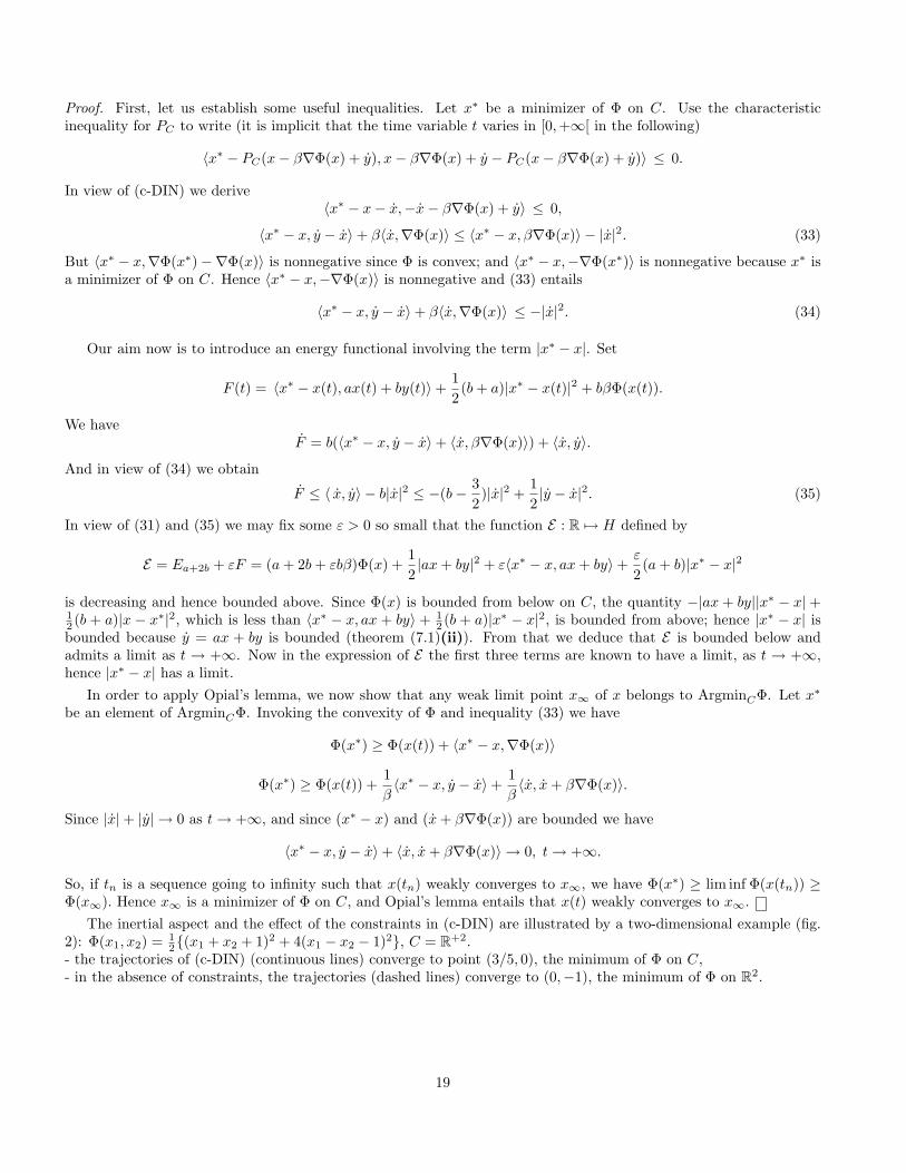
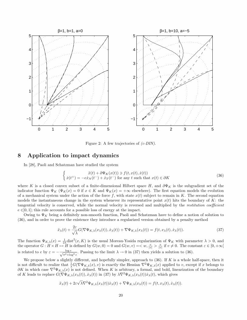
The inertial aspect and the effect of the constraints in (c-DIN) are illustrated by a two-dimensional example (fig.2): Φ(x1, x2) = 1

2(x1 + x2 + 1)2 + 4(x1 − x2 − 1)2, C = R+2.- the trajectories of (c-DIN) (continuous lines) converge to point (3/5, 0), the minimum of Φ on C,- in the absence of constraints, the trajectories (dashed lines) converge to (0,−1), the minimum of Φ on R2.

19

0 1 2 3 4 5

−1

0

1

2

3

4

5β=1, b=1, a=0

0 1 2 3 4 5

−1

0

1

2

3

4

5β=1, b=10, a=−5

Figure 2: A few trajectories of (c-DIN).

8 Application to impact dynamics

In [28], Paoli and Schatzman have studied the system

x(t) + ∂ΨK(x(t)) 3 f(t, x(t), x(t))x(t+) = −exN (t−) + xT (t−) for any t such that x(t) ∈ ∂K

(36)

where K is a closed convex subset of a finite-dimensional Hilbert space H, and ∂ΨK is the subgradient set of theindicator function ΨK (ΨK(x) = 0 if x ∈ K and ΨK(x) = +∞ elsewhere). The first equation models the evolutionof a mechanical system under the action of the force f , with state x(t) subject to remain in K. The second equationmodels the instantaneous change in the system whenever its representative point x(t) hits the boundary of K: thetangential velocity is conserved, while the normal velocity is reversed and multiplied by the restitution coefficiente ∈]0, 1]; this rule accounts for a possible loss of energy at the impact.

Owing to ΨK being a definitely non-smooth function, Paoli and Schatzman have to define a notion of solution to(36), and in order to prove the existence they introduce a regularized version obtained by a penalty method

xλ(t) +2ε√λ

G(∇ΨK,λ(xλ(t)), xλ(t)) +∇ΨK,λ(xλ(t)) = f(t, xλ(t), xλ(t)). (37)

The function ΨK,λ(x) = 12λdist2(x, K) is the usual Moreau-Yosida regularization of ΨK with parameter λ > 0, and

the operator G : H×H 7→ H is defined by G(w, 0) = 0 and G(w, v) =< w, v|v| > v

|v| if v 6= 0. The constant ε ∈ [0,+∞[

is related to e by ε = − log e√π2+log2 e

. Passing to the limit λ → 0 in (37) then yields a solution to (36).

We propose below a slightly different, and hopefully simpler, approach to (36). If K is a whole half-space, then itis not difficult to realize that 1

λG(∇ΨK,λ(x), v) is exactly the Hessian ∇2ΨK,λ(x) applied to v, except if x belongs to∂K in which case ∇2ΨK,λ(x) is not defined. When K is arbitrary, a formal, and bold, linearization of the boundaryof K leads to replace G(∇ΨK,λ(xλ(t)), xλ(t)) in (37) by λ∇2ΨK,λ(xλ(t))xλ(t), which gives

xλ(t) + 2ε√

λ∇2ΨK,λ(xλ(t))xλ(t) +∇ΨK,λ(xλ(t)) = f(t, xλ(t), xλ(t)).

20

For simplicity, assume henceforth that the exterior force reduces to a viscous friction: f(t, xλ(t), xλ(t)) = −αxλ(t),α ≥ 0. The preceding equation becomes

xλ + αxλ + 2ε√

λ∇2ΨK,λ(x)xλ +∇ΨK,λ(x) = 0.

This is (DIN) with β = 2ε√

λ. But this equation has to be given a sense since ΨK,λ is not twice differentiableeverywhere. The cure is to write it in the form (g-DIN) which is of first order in time and space (recall β = 2ε

√λ)

xλ + β∇ΨK,λ(xλ) +(α− 1β

)xλ +1β

yλ = 0

yλ +(α− 1β

)xλ +1β

yλ = 0(38)

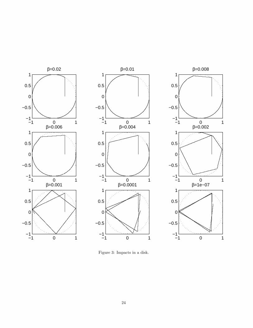
This system is numerically solvable as it stands. A few numerical experiments are reported in figure 3: K is theunit disk, α = 0, λ = 10−4, the system representative point starts from position (0.5, 0) with velocity (0, 0.1); thecoefficient β = 2ε

√λ runs through 0.02, 0.01, 0.008, 0.006, 0.004, 0.002, 0.001, 0.0001, 10−7, and correspondingly

the restitution coefficient e runs through 0, 0.16, 0.25, 0.37, 0.53, 0.73, 0.85, 0.98, 0.99998.The experiments display the whole range of possible shocks:

- completely anelastic shocks for β = 0.02: after the first shock the trajectory follows the boundary,- nearly perfectly elastic shocks for β = 10−7 (the theoretical trajectory in the disk - without penalization - is anequilateral triangle),- shocks with partial restitution of energy for intermediate values of β.

The purpose of these experiments is to illustrate the behaviour of the solutions of (38) and to suggest the latter asa theoretical regularization of (36). The numerical solution of (38) is prone to stiffness as λ becomes smaller (see [29]in this respect).

References

[1] M. Aassila, A new approach of strong stabilization of distributed systems, Differential and Integral Equations 11,n 2 (1998), 369-376.

[2] F. Alvarez, On the minimizing property of a second order dissipative system in Hilbert space, SIAM J. on Controland Optimization, 38, n 4, (2000), 1102-1119.

[3] F. Alvarez, H. Attouch, An Inertial Proximal Method for Maximal Monotone Operators via Discretization of aNonlinear Oscillator with Damping, Set-Valued Analysis, 9, Issue 1/2, March 2001, pp. 3-11.

[4] F. Alvarez and J.M. Perez, A dynamical system associated with Newton’s method for parametric approximationsof convex minimization problems, Applied Mathematics & Optimization, 38 (1998), 193-217.

[5] A. S. Antipin, Linearization method, in Nonlinear dynamic systems: Qualitative analysis and control (in Russian),Proc. ISA Russ. Acad. Sci., n 2, pp. 4-20, 1994; (english translation: Computational Mathematics and Modeling,n 1, 8, pp. 1-15, Jan. 1997).

[6] A. S. Antipin, Minimization of convex functions on convex sets by means of differential equations (in Russian),Differentsialnye Uravneniya, 30, n 9, pp. 1475-1486, Sep. 1994; (english translation: Differential Equations, 30,n 9, pp. 1365-1375, 1994).

[7] A. S. Antipin, A. Nedich, Continuous second-order linearization method for convex programming problems,Computational Mathematics and Cybernetics, Moscow University, 2, pp. 1-9, 1996.

[8] H. Attouch, F. Alvarez, The heavy ball with friction dynamical system for convex constrained minimizationproblems. Optimization (Namur, 1998), 25–35, Lecture Notes in Econom. and Math. Systems, 481, Springer,Berlin, 2000.

[9] H. Attouch, A. Cabot, P. Redont, The dynamics of elastic shocks via epigraphical regularization of a differentialinclusion. Barrier and penalty approximations, to appear in Advances in Mathematical Sciences and Applications,12, n 1 (2002).

21

[10] H. Attouch and R. Cominetti, A dynamical approach to convex minimization coupling approximation with thesteepest descent method, J. Differential Equations, 128 (2), (1996), 519-540.

[11] H. Attouch, X. Goudou and P. Redont, The heavy ball with friction method, I. The continuous dynamical system:global exploration of the global minima of a real-valued function by asymptotic analysis of a dissipative dynamicalsystem, Communications in Contemporary Mathematics, 2, n 1 (2000), 1-34.

[12] H. Attouch, P. Redont, The second-order in time continuous Newton method, Approximation Optimization andMathematical Economics, M. Lassonde ed., Proceedings of the Fifth International Conference on Approximationand Optimization in the Caribbean, Physica-Verlag, 2001, 25-36.

[13] J.P. Aubin and A. Cellina, Differential Inclusions: Set-Valued Maps and Viability Theory, Springer-Verlag, Berlin,1984.

[14] J.-B. Baillon, Un exemple concernant le comportement asymptotique de la solution du probleme du/dt+∂ϕ(u) =0, Journal of Functional Analysis, 28, 369-376 (1978).

[15] H. Brezis, Operateurs maximaux monotones, Mathematics Studies 5, North-Holland-American Elsevier, 1973.

[16] R.E. Bruck, Asymptotic convergence of nonlinear contraction semigroups in Hilbert space, Journal of FunctionalAnalysis, 18, (1975), 15-26.

[17] J. K. Hale, Asymptotic behavior of dissipative systems, Mathematical Surveys and Monographs 25, A.M.S.,Providence, R. I. (1987).

[18] A. Haraux, Semilinear hyperbolic problems in bounded domains, in Mathematical Reports (J. Dieudonne ed.) 3,Part I, Harwood Academic, Reading, UK, 1987.

[19] A. Haraux, Systemes dynamiques dissipatifs et applications, RMA 17, Masson, Paris, (1991).

[20] A. Haraux, M. Jendoubi, Convergence of solutions of second-order gradient-like systems with analytic nonlinear-ities, Journal of Differential Equations, 144, n 2 (1998).

[21] M. Jendoubi, Convergence of bounded and global solutions of the wave equation with linear dissipation andanalytic nonlinearity, J. Differential Equations, 144 (1998), 302-312.

[22] B. Kummer, Generalized Newton and NCP Methods: convergence, regularity, actions, Discussiones Mathemati-cae, Differential Inclusions, Control and Optimization, 20 (2000), 209-244.

[23] C. Lemarechal, J.-B. Hiriart-Urruty, Convex Analysis and Minimization Algorithms II: Advanced Theory andBundle Methods, Springer-Verlag, Berlin, 1993.

[24] S. Lojasiewicz, Une propriete topologique des sous-ensembles analytiques reels, in Colloques Internationaux duC.N.R.S. Les equations aux derivees partielles, 117 (1963).

[25] S. Lojasiewicz, Ensembles semi-analytiques, I.H.E.S. Notes, (1965).

[26] B. Mordukhovich, J. Outrata, On second-order subdifferentials and their applications, SIAM J. Optim., 12, N

1, pp. 139-169.

[27] Z. Opial, Weak convergence of the sequence of successive approximations for nonexpansive mappings, Bull. of theAmerican Math. Society, 73 (1967), 591-597.

[28] L. Paoli, M. Schatzman, Mouvement a un nombre fini de degres de liberte avec contraintes unilaterales: cas avecperte d’energie, Mod. Math. Anal. Num., 27 (1993), 673-717.

[29] L. Paoli, M. Schatzman, Ill-posedness in vibro-impact and its numerical consequences, ECOMAS conference 2000,Proceedings, to appear.

[30] J. Palis, W. de Melo, Geometric theory of dynamical systems, Springer, 1982.

22

[31] B. T. Polyak, Introduction to Optimization, Optimization Software, New York, 1987.

[32] R. Rockfellar, R. Wets, Variational Analysis, Springer, Berlin, 1998.

[33] L. Simon, Asymptotics for a class of non-linear evolution equations, with applications to geometric problems,Ann. of Math., 118, (1983), 525-571.

[34] S. Smale, A convergent process of price adjustment and global Newton methods, Journal of Mathematical Eco-nomics, 3 (1976), 107-120.

[35] R. Temam, Infinite dimensional dynamical systems in mechanics and physics, Applied mathematical sciences, 68,Springer, 1997.

23

−1 0 1−1

−0.5

0

0.5

1β=0.02

−1 0 1−1

−0.5

0

0.5

1β=0.01

−1 0 1−1

−0.5

0

0.5

1β=0.008

−1 0 1−1

−0.5

0

0.5

1β=0.006

−1 0 1−1

−0.5

0

0.5

1β=0.004

−1 0 1−1

−0.5

0

0.5

1β=0.002

−1 0 1−1

−0.5

0

0.5

1β=0.001

−1 0 1−1

−0.5

0

0.5

1β=0.0001

−1 0 1−1

−0.5

0

0.5

1β=1e−07

Figure 3: Impacts in a disk.

24