Kuramoto dynamics, glassy synchronization and rare regions in the human connectome - Pablo Villegas
Shinshu University
A Search for the Rare Leptonic DecaysB+ → µ+ νµ and B+ → e+ νe
Doctor Thesis
March 2007
Norihiko Satoyama
Division of Science and Technology,Shinshu University


�������
B� � � � �
B+ → µ+ νµ � B+ → e+ νe �� � � �
2007 � 3 �� � � �
� � � � � � � � ! " # $

Abstract
This thesis presents a search for the B+ → µ+νµ and B+ → e+νe decays followingΥ(4S )→ B+B−. In the Standard Model (SM) for the elementary particle physics, thesedecays proceed by annihilation to a virtual W boson, and these branching fractions areexpected. Search for these decays, therefore, can provide sensitivity to the SM param-eters and also act as a probe of physics beyond the SM. The data used in this analysiswere collected with the Belle detector at KEKB e+ (3.5 GeV) e− (8 GeV) asymmetric-energy collider. The data sample consists of an integrated luminosity of 253 fb−1 ac-cumulated at the Υ(4S ) resonance. The data sample corresponds to 276.6 × 10⁶ BBpairs.
As B+ → µ+νµ and B+ → e+νe decays are two-body decays, the signal chargedleptons have a fixed momentum in the signal B meson rest frame, which is higher thanmomenta of tracks from all other B decays. The lepton with high momentum is as-signed to the signal candidate lepton. All other particles are inclusively reconstructedto the companion B meson, which is the opposite side B meson of the signal side B me-son. The dominant background arises from the continuum processes and semileptonicB meson decays. In order to reduce such backgrounds, we use differences of eventtopology between signal and background events, and require a higher momentum trackfor signal candidate lepton and so on.
After the evetnt selection, we can find 12 (15) events in the signal region for themuon (electron) mode. There is no significant evidence for the both modes taking intoaccount the number of the background events we expected in the same region. We canset 90 % confidence level upper limits of the branching fractions to B(B+ → µ+νµ) <1.7 × 10⁻⁶ and B(B+ → e+νe) < 9.8 × 10⁻⁷. These upper limits are consistent with thepredictions of the SM. The upper limits are the best results to date.


Acknowledgements
First of all I would like to thank Prof. T. Takeshita and associate Prof. Y. Hasegawafor giving me the chance of join to Belle collaboration and I want to thank all of themembers in HE lab. in Shinshu University.
I would like to thank every member of the Belle collaboration and KEKB who hasbeen working hard to make the experiment run smoothly and successfully. This thesiswould not have been possible without their efforts. Especially I wish to thank everyonewho give me great suggestions for my study. When I started to analyze this decay modein 2003, I has very limited knowledge about experimental particle physics. They hasbeen always patient with me and guided me through every step of the way. I especiallythanks: T. Iijima, K. Ikado, K. Okabe and T. Hokuue in Nagoya University, I neverforget the days of meeting to report status at Nagoya University and via TV. I wouldlike to thank: S. Villa, I. Nakamura, G. R. Moloney, K. Abe, Y. Sakai, T. Browderand Simon I. Eidelman, the journal paper, which is required to submit this PhD thesis,could not been completed without your great helps. I am also grateful to Y. Miyazakifor your advises to carry on my study.
Last but least, I would like to thank my wife Ryoko, my daughter Nagomi, andmy parents Takashi and Yoshiko for always having faith in me and always being theresupporting me.
Norihiko Satoyama

Contents
1 Introduction 1
2 Leptonic Decay on Charged B Meson System 32.1 Standard Model . . . . . . . . . . . . . . . . . . . . . . . . . . . . . . . . . . . 32.2 Leptonic Decay of Charged B Meson . . . . . . . . . . . . . . . . . . . . . . . . 4
2.2.1 CKM Matrix . . . . . . . . . . . . . . . . . . . . . . . . . . . . . . . . 52.2.2 The Origin of the CKM Matrix . . . . . . . . . . . . . . . . . . . . . . . 52.2.3 Parametrization of the CKM Matrix . . . . . . . . . . . . . . . . . . . . 72.2.4 Unitarity Conditions of the CKM Matrix . . . . . . . . . . . . . . . . . 82.2.5 Constraining the Unitarity Triangle . . . . . . . . . . . . . . . . . . . . 92.2.6 Magnitude of Vub . . . . . . . . . . . . . . . . . . . . . . . . . . . . . . 112.2.7 SM Prediction . . . . . . . . . . . . . . . . . . . . . . . . . . . . . . . 122.2.8 Recent Result of Other Leptonic Decays . . . . . . . . . . . . . . . . . . 122.2.9 Theory Beyond the Standard Model . . . . . . . . . . . . . . . . . . . . 12
3 The Belle Experiments 153.1 The KEKB . . . . . . . . . . . . . . . . . . . . . . . . . . . . . . . . . . . . . 153.2 The Belle Detector . . . . . . . . . . . . . . . . . . . . . . . . . . . . . . . . . 17
3.2.1 Coordinate Systems . . . . . . . . . . . . . . . . . . . . . . . . . . . . 173.2.2 Beam Pipe . . . . . . . . . . . . . . . . . . . . . . . . . . . . . . . . . 183.2.3 Silicon Vertex Detector (SVD) . . . . . . . . . . . . . . . . . . . . . . . 193.2.4 Central Drift Chamber (CDC) . . . . . . . . . . . . . . . . . . . . . . . 213.2.5 Aerogel Cherenkov Counter (ACC) . . . . . . . . . . . . . . . . . . . . 243.2.6 Time of Flight Counter (TOF) . . . . . . . . . . . . . . . . . . . . . . . 273.2.7 Electromagnetic Calorimeter (ECL) . . . . . . . . . . . . . . . . . . . . 283.2.8 KL/µ Detector (KLM) . . . . . . . . . . . . . . . . . . . . . . . . . . . 313.2.9 Solenoid Magnet . . . . . . . . . . . . . . . . . . . . . . . . . . . . . . 333.2.10 Extreme Forward Calorimeter (EFC) . . . . . . . . . . . . . . . . . . . 34
3.3 Trigger and Data Acquisition System . . . . . . . . . . . . . . . . . . . . . . . . 343.3.1 Trigger . . . . . . . . . . . . . . . . . . . . . . . . . . . . . . . . . . . 343.3.2 Data Acquisition System . . . . . . . . . . . . . . . . . . . . . . . . . . 36
3.4 Monte Carlo Simulation . . . . . . . . . . . . . . . . . . . . . . . . . . . . . . 383.4.1 Event Generators . . . . . . . . . . . . . . . . . . . . . . . . . . . . . . 393.4.2 Simulation of Detector Response . . . . . . . . . . . . . . . . . . . . . . 39
3.5 Particle Reconstruction . . . . . . . . . . . . . . . . . . . . . . . . . . . . . . . 393.5.1 Reconstruction of Charged Particle Tracks . . . . . . . . . . . . . . . . . 393.5.2 Reconstruction of Photon Clusters . . . . . . . . . . . . . . . . . . . . . 40
v
vi CONTENTS
3.5.3 Charged Particle Identification . . . . . . . . . . . . . . . . . . . . . . . 403.5.4 Muon Identification . . . . . . . . . . . . . . . . . . . . . . . . . . . . . 403.5.5 Electron Identification . . . . . . . . . . . . . . . . . . . . . . . . . . . 413.5.6 Identification of Charged Hadrons: K/π Separation . . . . . . . . . . . . 42
4 Data Sets 47
5 Analysis 495.1 Particle Identification . . . . . . . . . . . . . . . . . . . . . . . . . . . . . . . . 49
5.1.1 KS reconstruction . . . . . . . . . . . . . . . . . . . . . . . . . . . . . . 495.1.2 Reconstruction of γ Conversion . . . . . . . . . . . . . . . . . . . . . . 515.1.3 Identification of Charged Particle . . . . . . . . . . . . . . . . . . . . . 515.1.4 Identification of Gamma (γ) . . . . . . . . . . . . . . . . . . . . . . . . 525.1.5 Signal Lepton Selection . . . . . . . . . . . . . . . . . . . . . . . . . . 535.1.6 Companion B Meson Reconstruction . . . . . . . . . . . . . . . . . . . 53
5.2 Event Selection . . . . . . . . . . . . . . . . . . . . . . . . . . . . . . . . . . . 545.2.1 Pre-selection . . . . . . . . . . . . . . . . . . . . . . . . . . . . . . . . 545.2.2 Definition of Regions . . . . . . . . . . . . . . . . . . . . . . . . . . . . 565.2.3 Signal Candidate Lepton . . . . . . . . . . . . . . . . . . . . . . . . . . 565.2.4 Continuum Suppression . . . . . . . . . . . . . . . . . . . . . . . . . . 595.2.5 Neutrino Reconstruction . . . . . . . . . . . . . . . . . . . . . . . . . . 605.2.6 Selection Optimization . . . . . . . . . . . . . . . . . . . . . . . . . . . 61
5.3 Signal Extraction . . . . . . . . . . . . . . . . . . . . . . . . . . . . . . . . . . 645.3.1 Probability Density Functions . . . . . . . . . . . . . . . . . . . . . . . 645.3.2 Likelihood Function . . . . . . . . . . . . . . . . . . . . . . . . . . . . 705.3.3 Unbinned Maximum Likelihood Fit . . . . . . . . . . . . . . . . . . . . 70
5.4 Systematic Uncertainties . . . . . . . . . . . . . . . . . . . . . . . . . . . . . . 715.4.1 Systematic Uncertainty of Signal Yield . . . . . . . . . . . . . . . . . . 715.4.2 Systematic Uncertainty of Mbc Distribution Shape . . . . . . . . . . . . 775.4.3 Summary of the Systematic Uncertainties . . . . . . . . . . . . . . . . . 77
5.5 Limits on Branching Fraction . . . . . . . . . . . . . . . . . . . . . . . . . . . . 775.5.1 Expected Sensitivity . . . . . . . . . . . . . . . . . . . . . . . . . . . . 80
6 Conclusion and Discussion 836.1 Conclusion . . . . . . . . . . . . . . . . . . . . . . . . . . . . . . . . . . . . . 836.2 Discussion . . . . . . . . . . . . . . . . . . . . . . . . . . . . . . . . . . . . . . 83
A Limits on Branching Fraction by Other Methods 87A.1 Additional Systematic Uncertainties . . . . . . . . . . . . . . . . . . . . . . . . 87
A.1.1 Systematic Uncertainty for Background Estimation . . . . . . . . . . . . 87A.2 Counting Method . . . . . . . . . . . . . . . . . . . . . . . . . . . . . . . . . . 91A.3 Unbinned Fit in the Signal Region . . . . . . . . . . . . . . . . . . . . . . . . . 92A.4 Sensitivities on Upper Limits . . . . . . . . . . . . . . . . . . . . . . . . . . . . 93
List of Figures
2.1 Feynman diagram for the leptonic decay on the charged Bd meson based on SMprediction. . . . . . . . . . . . . . . . . . . . . . . . . . . . . . . . . . . . . . . 4
2.2 The rescaled Unitarity Triangle . . . . . . . . . . . . . . . . . . . . . . . . . . . 92.3 Schematic view of the Unitarity Triangle and determination of its upper vertex,
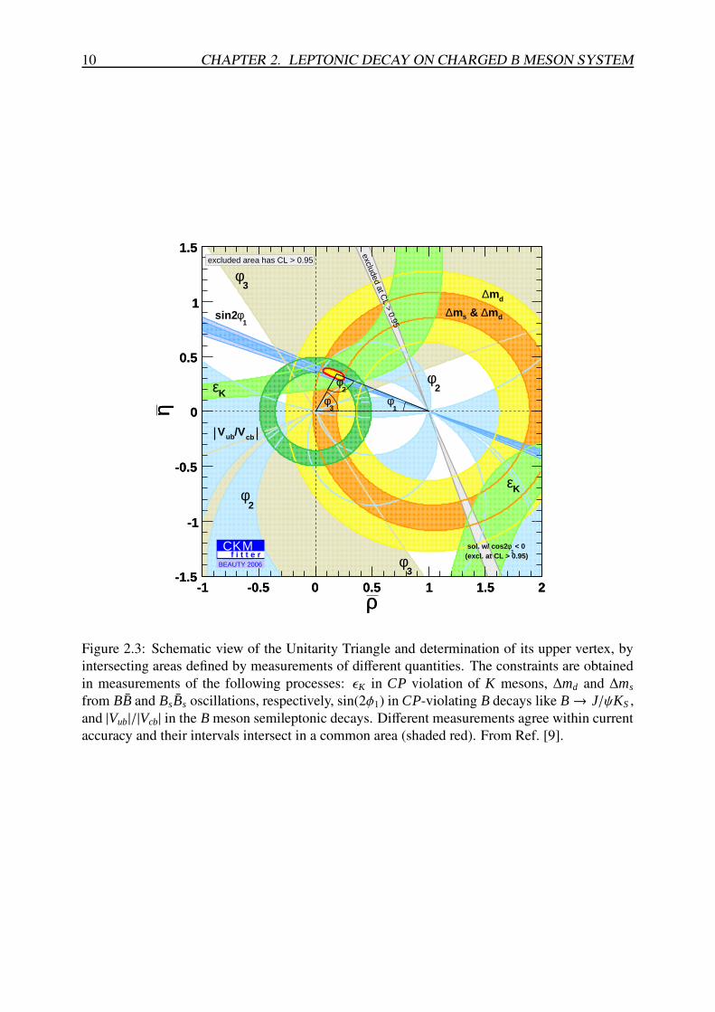
by intersecting areas defined by measurements of different quantities. The con-straints are obtained in measurements of the following processes: εK in CP vio-lation of K mesons, ∆md and ∆ms from BB and BsBs oscillations, respectively,sin(2φ1) in CP-violating B decays like B → J/ψKS , and |Vub|/|Vcb| in the B me-son semileptonic decays. Different measurements agree within current accuracyand their intervals intersect in a common area (shaded red). From Ref. [9]. . . . 10
2.4 Feynman diagram for the leptonic decay of the charged Bd meson via Higgsdoublet based on MSSM prediction. . . . . . . . . . . . . . . . . . . . . . . . . 13
3.1 The KEKB Storage rings, LER and HER, with the IP located in Tsukuba Exper-imental Hall. . . . . . . . . . . . . . . . . . . . . . . . . . . . . . . . . . . . . 16
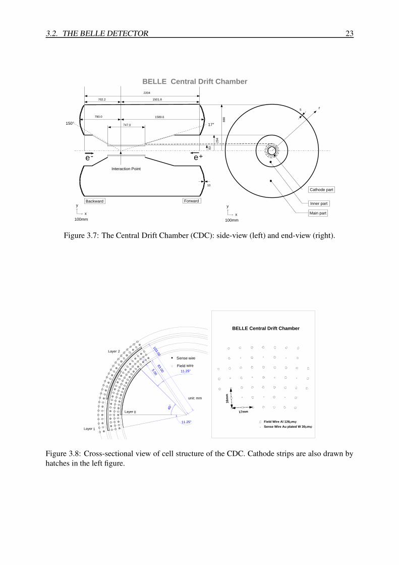
3.2 Cross section of e+e− → hadrons in a invariant mass range of 9.44− 10.62 GeV/c2. 173.3 Side view of the Belle detector. . . . . . . . . . . . . . . . . . . . . . . . . . . . 183.4 The cross section of the beryllium beam pipe at the interaction point. . . . . . . . 193.5 Schematic view of a Double Sided Silicon Detector. . . . . . . . . . . . . . . . . 203.6 Silicon vertex detector configurations for the SVD1 and the SVD2. . . . . . . . . 223.7 The Central Drift Chamber (CDC): side-view (left) and end-view (right). . . . . . 233.8 Cross-sectional view of cell structure of the CDC. Cathode strips are also drawn
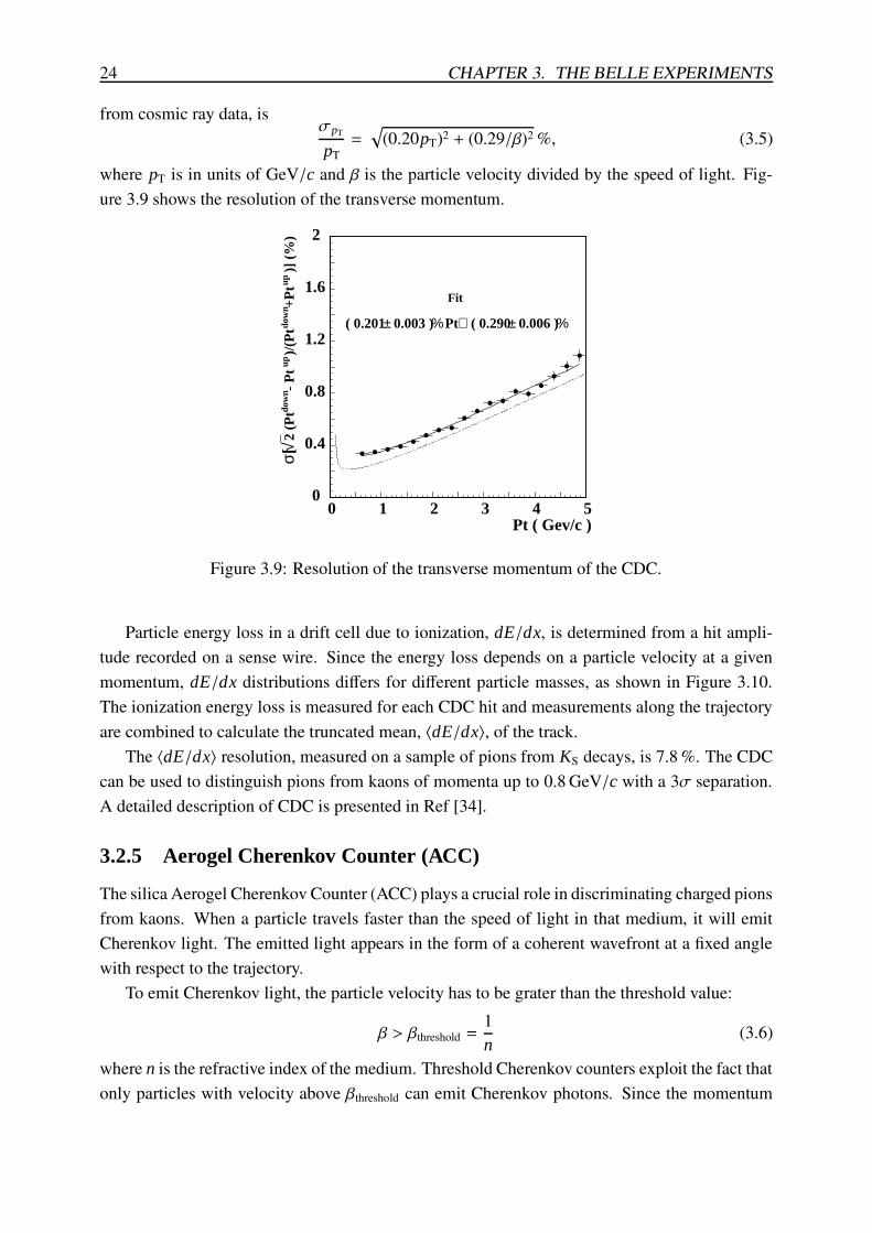
by hatches in the left figure. . . . . . . . . . . . . . . . . . . . . . . . . . . . . . 233.9 Resolution of the transverse momentum of the CDC. . . . . . . . . . . . . . . . 243.10 Truncated mean of dE/dx versus momentum The points are measurements taken
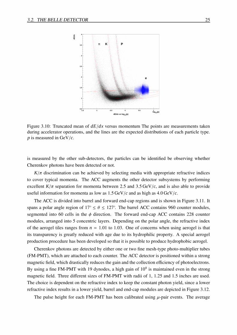
during accelerator operations, and the lines are the expected distributions of eachparticle type. p is measured in GeV/c. . . . . . . . . . . . . . . . . . . . . . . . 25
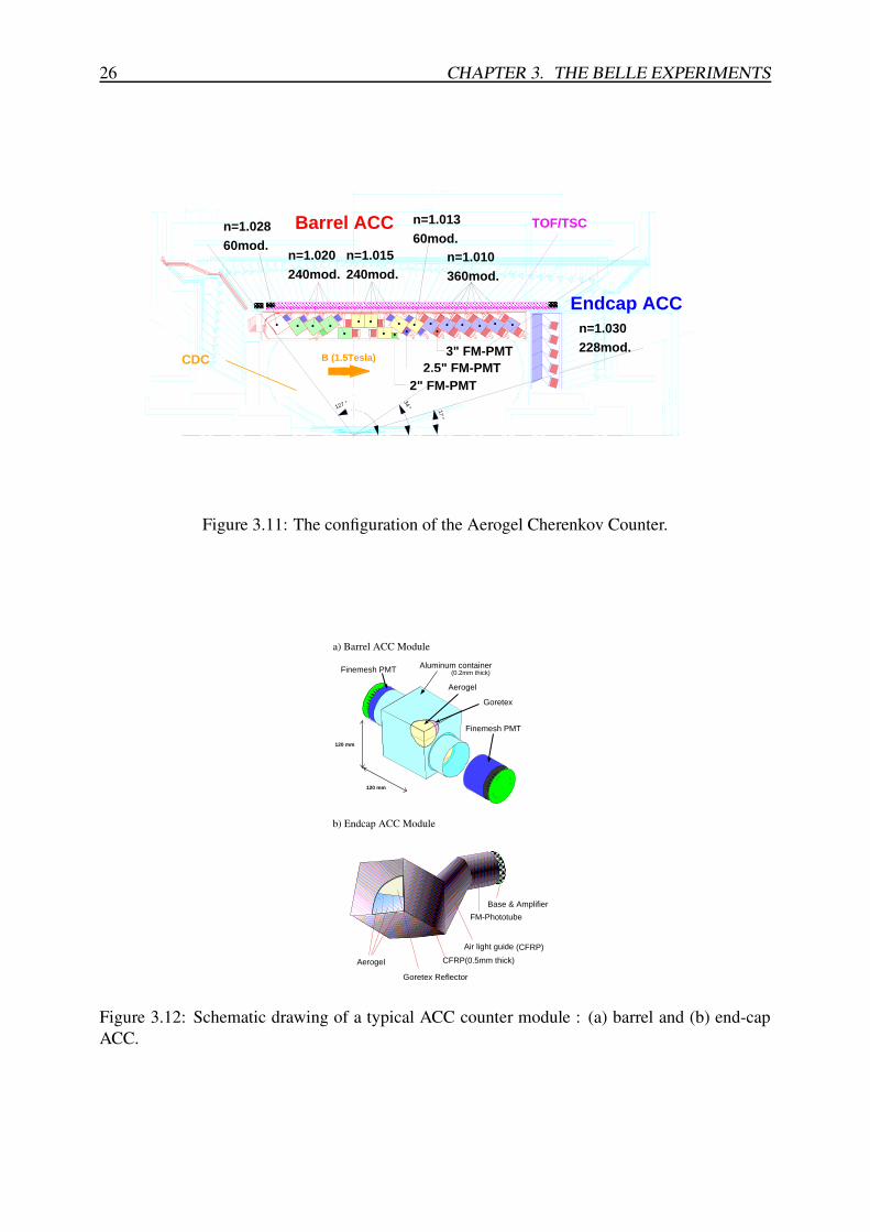
3.11 The configuration of the Aerogel Cherenkov Counter. . . . . . . . . . . . . . . . 263.12 Schematic drawing of a typical ACC counter module : (a) barrel and (b) end-cap
ACC. . . . . . . . . . . . . . . . . . . . . . . . . . . . . . . . . . . . . . . . . 263.13 Kaon efficiency and pion fake rate, measured with D∗+ → D0(→ Kπ)+π+ decays,
for the barrel region of the ACC. . . . . . . . . . . . . . . . . . . . . . . . . . . 273.14 Structure of the TOF/TSC module. The numbers in the figure are in units of mm. 28
vii
viii LIST OF FIGURES
3.15 Performance of TOF. (a) K/π separation performance of the TOF as a functionof momentum (µπ and µK are pion and kaon hypothesis probabilities, respec-tively). (b) Mass distribution from TOF measurements for particle momentabelow 1.2 GeV/c. The CDC momentum measurement and the velocity measure-ment by TOF are used. . . . . . . . . . . . . . . . . . . . . . . . . . . . . . . . 29
3.16 The configuration of Electromagnetic Calorimeter, with annular-shaped forwardand backward end-caps. . . . . . . . . . . . . . . . . . . . . . . . . . . . . . . . 30
3.17 Mechanical assembly of the ECL detector. . . . . . . . . . . . . . . . . . . . . . 30
3.18 Distribution of the energy deposit by electrons (dotted line), by positive pions(dashed line) and by negative pions (solid line) at 1 GeV/c. . . . . . . . . . . . . 31
3.19 Cross section of a KLM super-layer, consisting of two Resistive Plate Counterslayers. Ionizing particles instigate a discharge of HV plates, which induces sig-nals in the pickup strips. . . . . . . . . . . . . . . . . . . . . . . . . . . . . . . 32
3.20 A schematic diagram of Resistive Plate Counters in the KLM detector. . . . . . . 33
3.21 Contour plot of the measured magnetic field strength in the Belle detector. . . . . 33
3.22 An isometric view of the BGO crystals of the forward and backward EFC detectors. 35
3.23 The overview of the Level 1 trigger system. . . . . . . . . . . . . . . . . . . . . 37
3.24 The overview of the Belle DAQ system. . . . . . . . . . . . . . . . . . . . . . . 38
3.25 The efficiency for muon selection (left) and the pion fake rate (right) in the barrelas a function of the lab momentum, measured in e+e− → e+e−, µ+µ−. Opencircles for Prob(µ) > 0.1, closed circles for Prob(µ) > 0.9. From Ref [46]. . . . . 41
3.26 (a) Ratio of energy deposit to track momentum, E/p, (b) Transverse energyshape, E9/E25, (c) Rate of ionization energy loss dE/dx, for electrons (solidline) and pions (broken line). (d) The electron likelihood, Prob(e), for electrons(solid line) and pions (broken line). From Ref. [47]. . . . . . . . . . . . . . . . 43
3.27 The efficiency for electron selection (left) and the pion fake rate (right) as a func-tion of the momentum in the laboratory frame, measured in radiative Bhabhaevents. From Ref. [47]. . . . . . . . . . . . . . . . . . . . . . . . . . . . . . . . 44
3.28 Momentum coverage of kaon/pion separation at the Belle detector. . . . . . . . . 44
5.1 Particle identification (PID) flow chart: The boxes included MDST show theMDST data classes. The round boxes represent PID criteria. A particle namein a box shows an identified particle. The normal arrows show flows of particleidentification. Dash arrows show that two connected (round) boxes are related. . 50
5.2 Schema of duplicated tracks with a same charge track and an opposite chargetrack. Thick curve shows an original track and dashed curves show duplicatedtracks. Small x marks show hits for the CDC track finder. A large x mark showsthe IP position. . . . . . . . . . . . . . . . . . . . . . . . . . . . . . . . . . . . 52
5.3 pB` distribution for the signal MC samples, where pB
` represents the lepton mo-mentum in the B rest frame. . . . . . . . . . . . . . . . . . . . . . . . . . . . . . 54
LIST OF FIGURES ix
5.4 Mbc distributions of the companion B meson for the muon mode (right) and theelectron mode (left) just after the pre-selection have been applied. Points showthe on-resonance data, and solid histograms show the expected background dueto rare B→ Xu`ν decays (hatched, from MC); other BB events, mainly B→ Xc`ν
decays (cross-hatched, also from MC); and continuum events (light shaded, takenfrom scaled off-resonance data). The dashed histograms represent the signal aspredicted by the MC with arbitrary normalization. The following similar his-tograms have the same style. . . . . . . . . . . . . . . . . . . . . . . . . . . . . 55
5.5 ∆E distributions for the muon mode (right) and the electron mode (left) just afterpre-selection have been applied. The style of these histograms are the same asFigure 5.4. . . . . . . . . . . . . . . . . . . . . . . . . . . . . . . . . . . . . . 55
5.6 Two-dimensional distribution of ∆E vs Mbc for the signal MC events. The solidbox shows the fit region, the long-dashed box is the signal region and the short-dashed box is the Mbc sideband region. . . . . . . . . . . . . . . . . . . . . . . 56
5.7 The signal candidate lepton momentum in the B rest frame after the pre-selectionhave been applied. The arrows show the selection criteria. The histograms forthe signal MC are normalized to make thm visible. . . . . . . . . . . . . . . . . 57
5.8 Distributions of the cosine of the polar angle of the signal lepton direction. Thearrows show the selection criteria. We require the signal candidate lepton goesto the barrel region. . . . . . . . . . . . . . . . . . . . . . . . . . . . . . . . . . 58
5.9 The probability distribution of a charged kaon for a muon candidate after cos θµselection criterion have been applied. This selection is only for the muon mode. . 58
5.10 Event topology. . . . . . . . . . . . . . . . . . . . . . . . . . . . . . . . . . . . 595.11 Optimized Fisher discriminate momenta distribution. Dashed histogram shows
the signal MC. Light shaded histogram shows the qq (q = u, d, s, c) MC samples. 605.12 SFW distributions for the muon mode (left) and for the electron mode (right). . . 605.13 Distributions of the cosine of poler angle of the missing momentum in the labo-
ratory frame for the muon mode(left) and the electron mode(right). . . . . . . . 615.14 Transverse missing momentum distribution for the muon mode (left) and for the
electron mode (right). The selection criteria for cos θ` and cos θmissing have beenalready applied to these histograms. . . . . . . . . . . . . . . . . . . . . . . . . 62
5.15 Scatter plot of the significance (NS /√
NS + NB) vs the signal efficiency . . . . . . 625.16 Mbc − ∆E scatter plots for the on-resonance data for the muon mode (left) and
for the electron mode (right). Boxes are the signal regions and dotted boxes arethe fit regions. . . . . . . . . . . . . . . . . . . . . . . . . . . . . . . . . . . . 64
5.17 Mbc distributions in the fit region for the muon mode (left) and for the electron(right) after all selection criteria have been applied. The arrows show the signalregion. . . . . . . . . . . . . . . . . . . . . . . . . . . . . . . . . . . . . . . . 65
5.18 Signal PDF distributions for the muon mode (left) and for the electron mode(right). The points show the signal MC in the fit region after all the selectioncriteria have been applied. The solid lines show the signal PDF by fitting thesignal MC by the Crystal Ball function. . . . . . . . . . . . . . . . . . . . . . . 66
5.19 The background PDF for the muon mode (left) and for the electron mode (right).Theplots show the combined histograms for the background MC and off-resonancedata. . . . . . . . . . . . . . . . . . . . . . . . . . . . . . . . . . . . . . . . . . 68
x LIST OF FIGURES
5.20 Mbc distribution after all selection criteria have been applied. Dots show the MCsamples of the B meson decay in B → Xu`ν` background. Dashed lines are thesignal MC. Arrows indicate the edge of the signal region in Mbc. . . . . . . . . . 69
5.21 Mbc distribution for the on-resonance data in the ∆E sideband region after allselection criteria have been applied. The solid curves show the results fittedby the ARGUS function and the light curves show the curves of the ARGUSfunction with the 1-σ errors of the shape parameters. . . . . . . . . . . . . . . . 69
5.22 Fitted Mbc distribution in the Mbc sideband region by the ARGUS function as thebackground PDF. Dots show the on-resonance data. Hatched region is the Mbcsideband region and cross-hatched region is the signal region. . . . . . . . . . . 70
5.23 Likelihood distributions of the signal yield. The horizontal lines show the onesigma error of the signal yield. . . . . . . . . . . . . . . . . . . . . . . . . . . . 71
5.24 Mbc distributions for the events in the ∆E signal region, together with the fitresults (dotted lines). The solid curves are the background contributions. Thedashed curves are the signal contributions. The signal contribution in the electronmode is multiplied by a factor of −4 to make it visible on the plot. . . . . . . . . 72
5.25 The cos θ` distribution for the signal MC after the other selection criteria havebeen applied. . . . . . . . . . . . . . . . . . . . . . . . . . . . . . . . . . . . . 73
5.26 Pion momentum spectrum : These histogram show the momentum in the B restframe. Dashed histogram shows the muon momentum for B→ µν MC. . . . . . 74
5.27 Mbc distributions of companion B mesons for the combined sample of the MCevents and the off-resonance data. Entries of left figure are accepted by the muonmode selection criteria. Entries of right figure are rejected by the muon modeselection criteria. Dotted is the MC + off-resonance combined sample. Solidcurves show the fitted results by the combined function of the ARGUS functionand the Crystal Ball function. Dashed curves show the background component(ARGUS part). Light curves are the signal component by the Crystal Ball func-tion. . . . . . . . . . . . . . . . . . . . . . . . . . . . . . . . . . . . . . . . . . 75
5.28 Mbc distributions of companion B mesons for the on-resonance sample. Dottedshows the on-resonance data sample. The other configurations and styles are thesame as Figure 5.27. . . . . . . . . . . . . . . . . . . . . . . . . . . . . . . . . 75
5.29 Mbc distributions of companion B mesons for the combined sample of the MCevents and the off-resonance data. sample. The selection criteria for the elec-tron mode are applied. The other configurations and styles are the same as Fig-ure 5.27. . . . . . . . . . . . . . . . . . . . . . . . . . . . . . . . . . . . . . . 76
5.30 Mbc distributions of companion B mesons for the on-resonance sample. Dottedshows the on-resonance data sample. The selection criteria for the electron modeare applied. The other configurations and styles are the same as Figure 5.27. . . 76
5.31 Likelihood function dependence on the branching fractions. The solid and dottedcurves represent the likelihood functions without and with the inclusion of sys-tematic uncertainties, respectively. The arrows indicate the upper limits on thebranching fractions at 90 % confidence level. . . . . . . . . . . . . . . . . . . . 79
5.32 Confidence level versus branching fraction distribution for the muon mode (left)and for the electron mode (right). . . . . . . . . . . . . . . . . . . . . . . . . . . 80
5.33 Generated number of toy MC samples distributions as a function of events con-tained in a sample. The means indicate the expected number of the backgroundin the fit region in a sample and the RMS indicate its statistical errors. . . . . . . 81

LIST OF FIGURES xi
5.34 Computed upper limits of the branching fraction for the muon mode (left) andthe electron mode (right). . . . . . . . . . . . . . . . . . . . . . . . . . . . . . . 81
6.1 Changes of the upper limits of the branching fractions. The thick texts are theupper limits of the branching fractions with publication and the light texts arepreliminary results. . . . . . . . . . . . . . . . . . . . . . . . . . . . . . . . . . 84
A.1 Mbc − ∆E plane plot for the on-resonance data with the looser selection criteria. . 88A.2 Fitted Mbc distributions for the MC + off-resonance samples with the looser se-
lection criteria of the muon mode (left) and the electron mode (right). Solid linerepresents the fitting by the ARGUS function. Light lines correspond to errorsof the shape parameters. . . . . . . . . . . . . . . . . . . . . . . . . . . . . . . 89
A.3 Fitted Mbc distribution for the on-resonance sample with the looser selection cri-teria. Solid curve represents the fitting by the ARGUS function. Gray curvescorrespond to errors of the shape parameters. . . . . . . . . . . . . . . . . . . . 90
A.4 Fitted Mbc distribution for the on-resonance sample with the standard selectioncriteria. Solid curve represents the fitting by the ARGUS function. Gray curvescorrespond to errors of the shape parameters. . . . . . . . . . . . . . . . . . . . 90
A.5 Likelihood vs branching fraction for the muon mode(left) and the electron mode(right).Dashed curves are likelihood distributions of the branching fraction. The 90% C.L.arrows indeicate the branching fraction up to which the integration is 0.9. . . . . 92
A.6 Confidence level vs upper limit of the branching fraction for the muon mode(left) and the electron mode (right). Solid curves and light curves represent thecurves without and with smearing by systematic uncertainty. . . . . . . . . . . . 93
A.7 Toy MC study for the counting method : The trial is 3000 times. . . . . . . . . . 94A.8 Distributions of the expected upper limits of the branching fractions for the un-
binned maximum likelihood fit in the signal region. . . . . . . . . . . . . . . . . 95

List of Tables
3.1 Characteristics of the SVD1 and the SVD2 . . . . . . . . . . . . . . . . . . . . . 203.2 Main parameters of the solenoid magnet. . . . . . . . . . . . . . . . . . . . . . . 34
4.1 Table of data sets used for the analysis. The luminosities of the signal MC assumethat cross sections are 4.7 × 10⁻⁷ for the muon decay and 1.0 × 10⁻¹² for theelectron decay. . . . . . . . . . . . . . . . . . . . . . . . . . . . . . . . . . . . 47
5.1 Reconstruction criteria of KS mesons for various KS momentum ranges . . . . . . 495.2 Summary table of the signal region and the fit region . . . . . . . . . . . . . . . 575.3 Accumulated efficiencies for the muon decay mode [%]. We applied from the
top to the bottom of the event selection criteira in turn. “fit region” and “signalregion”, which are defined in section 5.2.2, show the efficiencies in the regionsafter all selection criteria have been applied. . . . . . . . . . . . . . . . . . . . 63
5.4 Accumulated efficiencies for the electron decay mode [%]. We applied from thetop to the bottom of the event selection criteria in turn. “fit region” and “signalregion”, which are defined in section 5.2.2, show the efficiencies in the regionsafter all selection criteria have been applied. . . . . . . . . . . . . . . . . . . . 63
5.5 Parameters determined by the fit in the Crystal Ball function for the muon modeand the electron mode. . . . . . . . . . . . . . . . . . . . . . . . . . . . . . . . 66
5.6 Looser selection criteria. . . . . . . . . . . . . . . . . . . . . . . . . . . . . . . 675.7 The background components’ ratio. . . . . . . . . . . . . . . . . . . . . . . . . 675.8 Signal yield summary table. . . . . . . . . . . . . . . . . . . . . . . . . . . . . 715.9 Systematic uncertainties of the lepton identification dependent on the lepton mo-
mentum (p` [GeV/c]) and the direction (θ) with respect to the beam axis. . . . . . 735.10 Comparison of efficiencies for fully reconstructed B→ Dπ samples . . . . . . . 775.11 Parameter errors for the signal PDF (Crystal Ball function) and background PDF
(ARGUS) and their contributions for the signal yield. Total systematic uncer-tainty is calculated from the square-root of the quadratic sum of the contributions. 78
5.12 Summary of systematic uncertainties . . . . . . . . . . . . . . . . . . . . . . . . 78
A.1 Uncertainties for the background estimation by statistics of the MC + off-resonancesample with the looser selection criteria. . . . . . . . . . . . . . . . . . . . . . . 88
A.2 Uncertainties for the background estimation from the on-resonance data statisticsuncertainties. . . . . . . . . . . . . . . . . . . . . . . . . . . . . . . . . . . . . 88
A.3 Ratio of the integration values of the signal region and the sideband region withthe looser and the standard selection criteria for the muon mode. . . . . . . . . . 90
A.4 Ratio of the integration values of the signal region and the sideband region withthe looser and the standard selection criteria for the electron mode. . . . . . . . . 91
xiii

LIST OF TABLES i
A.5 Uncertainties for the background estimation from the statistics uncertainties ofthe on-resonance sample. . . . . . . . . . . . . . . . . . . . . . . . . . . . . . . 91
A.6 Sensitivities of the upper-limit-extraction methods. . . . . . . . . . . . . . . . . 94

Chapter 1
Introduction
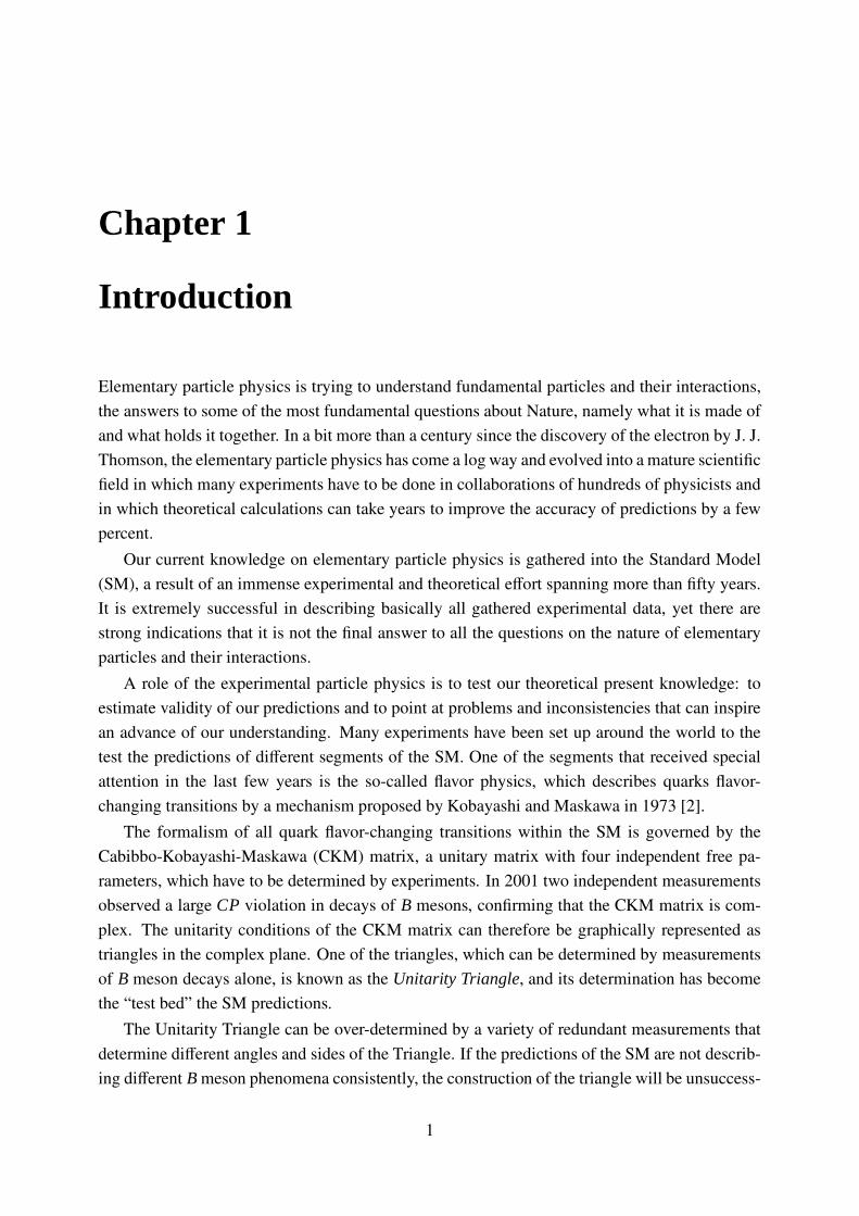
Elementary particle physics is trying to understand fundamental particles and their interactions,the answers to some of the most fundamental questions about Nature, namely what it is made ofand what holds it together. In a bit more than a century since the discovery of the electron by J. J.Thomson, the elementary particle physics has come a log way and evolved into a mature scientificfield in which many experiments have to be done in collaborations of hundreds of physicists andin which theoretical calculations can take years to improve the accuracy of predictions by a fewpercent.
Our current knowledge on elementary particle physics is gathered into the Standard Model(SM), a result of an immense experimental and theoretical effort spanning more than fifty years.It is extremely successful in describing basically all gathered experimental data, yet there arestrong indications that it is not the final answer to all the questions on the nature of elementaryparticles and their interactions.
A role of the experimental particle physics is to test our theoretical present knowledge: toestimate validity of our predictions and to point at problems and inconsistencies that can inspirean advance of our understanding. Many experiments have been set up around the world to thetest the predictions of different segments of the SM. One of the segments that received specialattention in the last few years is the so-called flavor physics, which describes quarks flavor-changing transitions by a mechanism proposed by Kobayashi and Maskawa in 1973 [2].
The formalism of all quark flavor-changing transitions within the SM is governed by theCabibbo-Kobayashi-Maskawa (CKM) matrix, a unitary matrix with four independent free pa-rameters, which have to be determined by experiments. In 2001 two independent measurementsobserved a large CP violation in decays of B mesons, confirming that the CKM matrix is com-plex. The unitarity conditions of the CKM matrix can therefore be graphically represented astriangles in the complex plane. One of the triangles, which can be determined by measurementsof B meson decays alone, is known as the Unitarity Triangle, and its determination has becomethe “test bed” the SM predictions.
The Unitarity Triangle can be over-determined by a variety of redundant measurements thatdetermine different angles and sides of the Triangle. If the predictions of the SM are not describ-ing different B meson phenomena consistently, the construction of the triangle will be unsuccess-
1

2 CHAPTER 1. INTRODUCTION
ful and would be a clear indication of physics beyond the SM. To spot inconsistencies betweenpredictions for different processes, however, the measurements have to achieve high accuracyand well understood errors.
The measurement of angle φ1 in 2001, which was determined by observed CP violation indecays of B mesons, opened a new theoretically clean way of testing the SM predictions. Theside of the Unitarity Triangle that lies opposite to the angle φ1 is determined by the measurementof the matrix element |Vub|, one of the smallest CKM matrix elements. While the measurementof φ1 includes loops in its Feynman diagrams that are sensitive to possible new contributions ofphysics beyond the SM, the measurement of |Vub| can be determined from tree-type diagramsthat are insensitive to new physics. Comparison of the measurements of φ1 and |Vub| is thereforean excellent opportunity to test the consistency of the SM predictions.
Two e+e− colliders with asymmetric energies of beams (so-called B factories), KEKB andPEP-II, have been set up at KEK (High Enegy Accelerator Research Organization) and SLAC(Stanford Linear Accelerator Center) respectively, to perform precise quantitative studies of B
mesons decays. They host the experiments Belle and BaBar, whose main goal is a precise mea-surement of CP asymmetries in B meson decays. The B mesons are produced in pairs fromdecays of the Υ(4S ) resonance, and the two experiments have so far managed to collect severalhundred million decays of B meson pairs. Such a large data sample enables the physicists to per-form a large set of various measurements and to search rare decays from B meson, The variousmeasurements and searches are also available to verify the SM and search for new physics. Theexperiments Belle and BaBar have already observed some new rare decays from B meson. How-ever there are many expected rare decays by the SM and they have not been observed yet. Thisthesis describes on the analysis of two rare decays from charged B meson which have not beenobserved yet, B+ → µ+νµ and B+ → e+νe, and the analysis described in the thesis was performedon a sample collected by the Belle detector at KEK in Japan.
The thesis is organized as follows: in the chapter 2 we first discuss the theory of the SMand the motivation for our study. In the chapter 3 we present the experimental environmentand the general event reconstruction techniques used at the Belle detector. We introduce datasamples analyzed in our study in the chapter 4. We describe our analysis in the chapter 5. Inthe section 5.1 in the analysis chapter, we present the techniques of the particle identificationand particle reconstructions. In the section 5.2 the event selection is described. After the eventselection, we mentioned how many the signal yields are expected and the method to extract thesignal yield in the section 5.3. The number of the expected backgrounds is also described in thesame section. The systematic uncertainties are described in the section 5.4. In the section 5.5,we set the upper limits on branching fractions for both modes as our analysis results. In the lastchapter 6 we come to the conclusion and review the results and propose future improvements.
Chapter 2
Leptonic Decay on Charged B MesonSystem
In this chapter we review why we try to search for the leptonic decay. The search is importantfor our understanding of the validity of the Standard Model (SM) predictions and may give thenew physics beyond the SM. The SM is firstly introduced and we explain the SM predictions forthe leptonic decay on charged B meson system. A theory beyond the SM is also introduced.
2.1 Standard Model
The Standard Model (SM) is a set of gauge theories that explain how elementary particles inter-act with each other through basic interactions. The elementary particles are, according to theirquantum-mechanical properties, separated into three groups: fermions, gauge bosons, and thepredicted Higgs particle. There are twelve elementary fermions (with their twelve antiparticles): six leptons and six quarks, which are grouped into three generations,
(
νe
e
) (
νµµ
) (
νττ
)
,
(
ud
) (
cs
) (
tb
)
.
The elementary particles in the SM interact through three interactions∗ : weak, strong andelectro-magnetic, by exchanging appropriate gauge bosons pertaining to the interaction. Thegauge group describing the interactions is S U(3)C × S U(2)L ×U(1)Y . The group S U(3) denotesQuantum Chromodynamics (QCD), which governs the strong interaction among quarks, whileunified electro-weak interactions are characterized by the gauge group S U(2)L × U(1)Y .
The SM is a result of a joint effort of theoretical and experimental physicists over the last 50years. Its predictions are continuously confronted by new data and experimental methods. Untilrecently, all the measured results could be described, within theoretical and experimental errors,
∗A unified theory including gravitational interaction has not been achieved yet. Since the gravitational interactionis much weaker than the other three at elementary particle level, its omission does not effect the applicability of theSM predictions to phenomena at the energies obtainable at accelerators today.
3

4 CHAPTER 2. LEPTONIC DECAY ON CHARGED B MESON SYSTEM
by the SM predictions. Nevertheless, physicists expect that the SM is not the final theory andthey will eventually observe physical processes which need to be described by theories beyondthe SM. Recently, the neutrino oscillations have been experimentally confirmed, and shown thatneutrinos are not massless particles: to include this, the SM needs to be extended. Other con-ceptual problems, for example the so-called gauge hierarchy problem, a large number of freeparameters of the SM and some cosmological observations hint at the possibility of physicalprocesses that cannot be satisfactorily explained and described by the SM.
There is a wide range of proposed elementary particle processes in which the contributionsbeyond the SM can arise, and there are important tests of the SM predictions. A set of tests iscurrently performed in the weak decays of heavy mesons, of which the search for rare decaysplays an important part.
2.2 Leptonic Decay of Charged B Meson
The leptonic decay of a charged B belongs to a weak decay. One way to test the SM predictionsis to look at the weak interaction. The weak interaction is described within the SM with anexchange of W± and Z0 bosons. Both quarks and leptons are affected by the weak interaction,and it is the only interaction of neutrinos. Weak decays are also the only ones to depend on quarkflavor. The leptonic decay on a meson system also indicates the annihilation of two quarks, ofwhich the meson consists, into a W± boson and pair creation of a lepton and a neutrino fromthe W± boson. Figure 2.1 shows the Feynman diagram for the leptonic decay of the charged B
meson based on the SM prediction.
W ∗
Vub, fB
b
u
B+
`+
ν`
Figure 2.1: Feynman diagram for the leptonic decay on the charged Bd meson based on SMprediction.
The amplitude for the Feynman diagram is of the form
M = GF√2
Vub[uγu(1 − γ5)b][`γu(1 − γ5)ν] (2.1)
where GF is the Fermi coupling constant, Vub is one of the Cabibbo-Kobayashi-Maskawa matrixelements and u, b, ` and ν correspond to the wave functions of themselves. The standard V-A
2.2. LEPTONIC DECAY OF CHARGED B MESON 5
term induces B+ → `+ν decay via axial-vector current, with
< 0|uγuγ5b|B+ >= i fBpµB. (2.2)
Equation 2.1 is given asM = GF√
2Vub fBm`[`γu(1 − γ5)ν], (2.3)
where this amplitude is proportional to lepton mass (m`) (helicity suppression). Then the branch-ing fraction is calculated from Equation 2.3 as
B(B+ → `+ν`) =G2
FmBm2`
8π
(
1 −m2`
m2B
)2
f 2B |Vub|2τB, (2.4)
where mB is B meson mass, |Vub| is the magnitude of one of the Cabibbo-Kobayashi-Maskawamatrix elements, and τB is the B+ lifetime. The Vub is introduced in the following sections.
2.2.1 CKM Matrix
Vub is one of the Cabibbo-Kobayashi-Maskawa (CKM) matrix elements. The theory of the CKMis introduced from this section.
The transformation property under the electroweak gauge group S U(2)L × U(1)Y is differentfor left and right-handed fermions. The right-handed components of the leptons and quarks aresinglets under the weak symmetry S U(2)L, while the left-handed components transform as weakS U(2)L doublets:
(
ud′
)
L
(
cs′
)
L
(
tb′
)
L
. (2.5)
The quark mass states are not eigen-states of the weak interaction, therefore the states coupledin the doublets need to be rotated into the weak eigen-state frame, where the rotated states aredenoted with a prime (see Equation 2.5). This rotation was first proposed by Cabibbo in 1963 [1]for the case of three quarks that were known at that time, and was later generalized for three quarkgenerations with six quark flavors by Kobayashi and Maskawa (1973) [2], by the introduction ofthe Cabibbo-Kobayashi-Maskawa (CKM) mixing matrix.
The model was proposed when only three quarks were known and was able to predict theexistence of six quarks. A large CP violation is arisen in B meson decays [3].
2.2.2 The Origin of the CKM Matrix
The elementary particles in the SM are massless, since mass terms in the Lagrangian break thelocal gauge invariance. But it was shown that by introducing scalar Higgs fields the particles can,after spontaneous symmetry breaking (SSB), acquire mass by coupling with the Higgs fields. Thederivation follows the steps described in Ref. [4].
The mass of a fermion is obtained from the Yukawa coupling between a fermionic fields(e, ν, u or d) and Higgs field (φ):
LY = −Cei j( ¯
iLφ)e′jR − Cui j(qiLφ
c)u′jR − Cdi j(qiLφ)d′jR + h.c., (2.6)
6 CHAPTER 2. LEPTONIC DECAY ON CHARGED B MESON SYSTEM
where u′ and d′ represent vectors of all up-type and down-type quarks, e is one of the chargedleptons, and ` and q represent one of the leptons and one of the quarks, respectively. The indicesi and j denote the generation of the quark or the lepton, and subscripts L and R denote theleft-handed and right-handed particle fields, respectively. The coefficients C i j are three 3 × 3matrices that determine the strength of the Yukawa couplings between fermions and Higgs fields( f represents either a charged lepton, an up-type quark or a down-type quark) and can be arbitrarycomplex matrices. After SSB with weak isospin doublet Higgs fields, the Higgs doublet can bewritten as follows:
φ(c) → 1√
2(v + H)χ(c), χ =
(
01
)
, (2.7)
where the Higgs field is split into its vacuum expectation value v and the remaining Higgs fieldH, which obtaines its mass in the process of SSB. Inserting Equation 2.7 into Equation 2.6 weobtain the following form of the Yukawa part of the Lagrangian:
LY = −(
1 + Hv
)
(e′LM′ee′R + u′LM′
uu′R + d′LM′dd′R + h.c.). (2.8)
The non-diagonal mass matrices are directly connected to the Yukawa coupling coefficients inEquation 2.6:
M′f =
v√
2C f
i j. (2.9)
Since the matrices representing the Yukawa coupling constants C fi j can be arbitrary, the mass
matrices are by default neither diagonal nor symmetric. The absence of right-handed neutrinosresults in a diagonalized mass matrix for leptons (M′
e), which means that the lepton fields inthe electroweak Lagrangian have also definite mass. This is not the case for quark fields: thequark fields u′ and d′ in the Yukawa Lagrangian in Equation 2.6 do not have definite mass. Toobtain the physical states with definite mass, we preform a unitary transformation using unitarymatrices S and T to diagonalize the quark mass matricesM′
q:
M′q = S †qMqS qTq. (2.10)
The matrices S q transform the gauge (interaction) quark eigen-statesψ′q into the mass eigen-statesψ f :
ψqL ≡ S qψ′qL (2.11)
ψqR ≡ S qTqψ′qR. (2.12)
The fact that the interaction quark eigen-states are not the same as the mass eigen-states has im-portant consequences on the electroweak interactions, which can be derived from the Lagrangianterm:
L = ΨLiγuDLµΨL + ΨRiγuDR
µΨR. (2.13)
After explicitly writing the covariant derivatives DLµ and DR
µ , we obtain three types of electroweakinteractions, weak charged, weak neutral and electromagnetic interactions. The weak neutral and
2.2. LEPTONIC DECAY OF CHARGED B MESON 7
electromagnetic interactions are not flavor-changing, therefore they have the same form in bothphysical and interaction bases.
The weak charged interaction, which plays the most important role in semileptonic decays, onthe other hand has a different form in the two bases. The corresponding term int the Lagrangianof the weak charged interaction is of the form:
Lw.c. = − g√
2(Jµ†Wµ + JµW†
µ), (2.14)
where the weak charged current Jµ is coupled to a charged massive boson field Wµ and thestrength of the interaction is determined by the coupling constant g.
The quark contribution to this charged current Jµw.c. is:
J†w.c. = u′Lγµd′L = uLγµS µS
†ddL = uLγµVCKMdL. (2.15)
We define the Cabibbo-Kobayashi-Maskawa matrix VCKM ≡ S uS †d, which is a unitary matrixintroduced by Kobayashi and Maskawa in 1973 [2] and rotating the down-type quark states,while leaving the up-type quarks unchanged: d′ = VCKMd.
d′
s′
b′
=
Vud Vus Vub
Vcd Vcs Vcb
Vtd Vts Vtb
dsb
, (2.16)
so that the charged current can be written as:
J†c.c. = (uct)L γµ
Vud Vus Vub
Vcd Vcs Vcb
Vtd Vts Vtb
dsb
L
. (2.17)
The weak charged interaction involves a change of quark flavor between the up-type and down-type quarks, and the VCKM matrix elements determine the strength of the coupling of up-typequarks to down-type quarks. The probability for a flavor transition of the i-th generation up-typequark to a j-th generation down-type quark is proportional to the CKM matrix element squared,|Vi j|2.
2.2.3 Parametrization of the CKM Matrix
The CKM matrix is in general a complex n × n matrix, where n is the number of generationsof elementary particles. In the case of three generations there are 18 parameters, but due tounitarity conditions only nine of them are independent, and further five phases can be removedby appropriate rotations of the quark fields, therefore 4 independent parameters remains. TheCKM matrix can thus be parameterized with four parameters (three real angles and one complexphase). These four parameters are free parameters of the SM.
The standard parameterization [5] of the matrix is given by:
VCKM =
c12c13 s12c13 s13eiδ
−s12c23 − c12s23s13eiδ c12c23 − s12s23s13eiδ s23c13
s12s23 − c12c23s13eiδ −s23c12 − s12c23s13eiδ c23c13
, (2.18)
8 CHAPTER 2. LEPTONIC DECAY ON CHARGED B MESON SYSTEM
where ci j = cos θi j, si j = sin θi j where i, j = 1, 2, 3 label the quark generation and δ is the phase.All of the ci j and si j can be chosen to be positive and δ may vary in the range 0 ≤ δ ≤ 2π.
One of the more common and illustrative parameterizations is the Wolfenstein parameteriza-tion [6], which takes into account the hierarchical structure of the sizes of CKM matrix elements:
VCKM =
1 − λ2
2 λ Aλ3(ρ − iη)−λ 1 − λ2
2 Aλ2
Aλ3(1 − ρ − iη) −Aλ2 1
+ O(λ4). (2.19)
It is an expansion in powers of λ ≡ |Vus| = 0.2200± 0.0026 [7]. A = 0.85± 0.09 and λ are knownto high precision, while %(≡ Aλ3ρ + O(λ4)), and η (Equation 2.21) are not well determined yet.If we define
s12 = λ; s23 = Aλ2; s13eiδ = Aλ3(% − iη), (2.20)
it follows that% =
s13
s12s23cos δ, η = s13
s12s23sin δ. (2.21)
We can write the CKM matrix parameterization that is correct to O(λ7) [8]:
VCKM =
1 − λ2
2 −18λ
4 λ + O(λ7) Aλ3(% − iη)−λ + 1
2 A2λ5[1 − 2(% + iη)] 1 − λ2
2 −18λ
4(1 + 4A2) Aλ2 + O(λ8)Aλ3(1 − % − iη) −Aλ2 + 1
2 Aλ4[1 + 2(% + iη)] 1 − 12 A2λ4
, (2.22)
where we have, by including the corrections of the order of λ2, defined two parameters:
% = %
(
1 − λ2
2
)
, η = η
(
1 − λ2
2
)
. (2.23)
2.2.4 Unitarity Conditions of the CKM Matrix
The CKM matrix VCKM is unitary by construction, VCKMV†CKM = I, which leads to the followingrelations amongst its elements:
∑
i
Vi jV∗ik = δ jk. (2.24)
Since the matrix elements of VCKM are in general complex, the unitarity conditions for differentrows ( j , k) can be illustrated as triangles in the complex plane. The triangle formed from theunitarity relation imposed on the first and third columns has specail significance since it is oneof the few such triangles with sides of roughly the same length (O(λ3)). The relation is given by
VudV∗ub + VcdV∗cb + VtdV∗tb = 0, (2.25)
and determines the so called Unitarity Triangle. For convenience, we normalize one of the sidesby dividing the relation in Equation 2.25 with |VcdV∗cb| and choose a phase convention so thatVcdV∗cb is real. The vertices along the normalized side are fixed at (0, 0) and (0, 1), while theremaining vertex has the coordinates (%, η), and needs to be determined by experiments (SeeFigure 2.2).
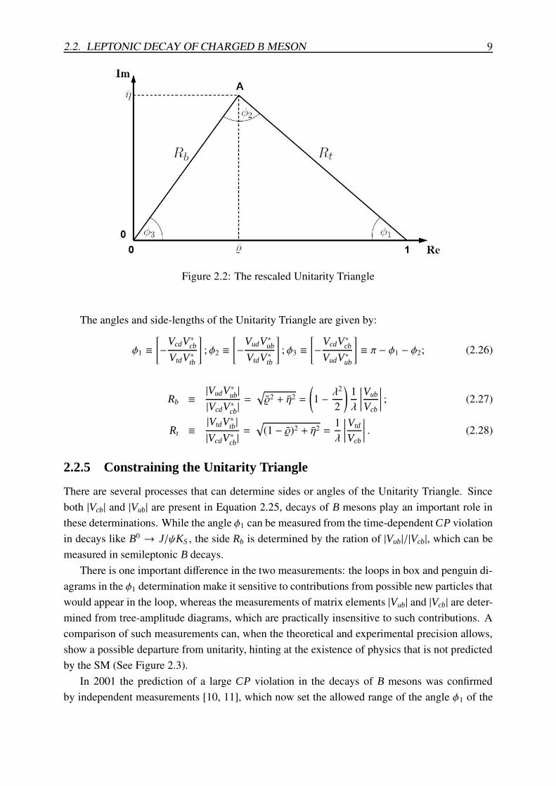
2.2. LEPTONIC DECAY OF CHARGED B MESON 9
Figure 2.2: The rescaled Unitarity Triangle
The angles and side-lengths of the Unitarity Triangle are given by:
φ1 ≡[
−VcdV∗cb
VtdV∗tb
]
; φ2 ≡[
−VudV∗ub
VtdV∗tb
]
; φ3 ≡[
−VcdV∗cb
VudV∗ub
]
≡ π − φ1 − φ2; (2.26)
Rb ≡|VudV∗ub||VcdV∗cb|
=√
%2 + η2 =
(
1 − λ2
2
)
1λ
∣
∣
∣
∣
∣
Vub
Vcb
∣
∣
∣
∣
∣
; (2.27)
Rt ≡|VtdV∗tb||VcdV∗cb|
=√
(1 − %)2 + η2 =1λ
∣
∣
∣
∣
∣
Vtd
Vcb
∣
∣
∣
∣
∣
. (2.28)
2.2.5 Constraining the Unitarity Triangle
There are several processes that can determine sides or angles of the Unitarity Triangle. Sinceboth |Vcb| and |Vub| are present in Equation 2.25, decays of B mesons play an important role inthese determinations. While the angle φ1 can be measured from the time-dependent CP violationin decays like B0 → J/ψKS , the side Rb is determined by the ration of |Vub|/|Vcb|, which can bemeasured in semileptonic B decays.
There is one important difference in the two measurements: the loops in box and penguin di-agrams in the φ1 determination make it sensitive to contributions from possible new particles thatwould appear in the loop, whereas the measurements of matrix elements |Vub| and |Vcb| are deter-mined from tree-amplitude diagrams, which are practically insensitive to such contributions. Acomparison of such measurements can, when the theoretical and experimental precision allows,show a possible departure from unitarity, hinting at the existence of physics that is not predictedby the SM (See Figure 2.3).
In 2001 the prediction of a large CP violation in the decays of B mesons was confirmedby independent measurements [10, 11], which now set the allowed range of the angle φ1 of the
10 CHAPTER 2. LEPTONIC DECAY ON CHARGED B MESON SYSTEM
ρ-1 -0.5 0 0.5 1 1.5 2
η
-1.5
-1
-0.5
0
0.5
1
1.5
2φ
1φ
3φ
ρ-1 -0.5 0 0.5 1 1.5 2
η
-1.5
-1
-0.5
0
0.5
1
1.5
3φ
3φ
2φ
2φ
dm∆
Kε
Kε
dm∆ & sm∆
cb/VubV
1φsin2
< 01
φsol. w/ cos2(excl. at CL > 0.95)
excluded area has CL > 0.95
excluded at CL > 0.95
BEAUTY 2006
CKMf i t t e r
Figure 2.3: Schematic view of the Unitarity Triangle and determination of its upper vertex, byintersecting areas defined by measurements of different quantities. The constraints are obtainedin measurements of the following processes: εK in CP violation of K mesons, ∆md and ∆ms
from BB and BsBs oscillations, respectively, sin(2φ1) in CP-violating B decays like B→ J/ψKS ,and |Vub|/|Vcb| in the B meson semileptonic decays. Different measurements agree within currentaccuracy and their intervals intersect in a common area (shaded red). From Ref. [9].
2.2. LEPTONIC DECAY OF CHARGED B MESON 11
Triangle (see Figure 2.3). The measurement of the angle φ1 is done by observing the time-dependent asymmetries between the decays of B and B mesons to a common final state. Theasymmetries arise due to the interference between the amplitudes for the direct decay and fora decay with the mixing of the B meson. The decay whose asymmetry is the most accuracypredicted by the theory B0 → J/ψKS. It is a decay with relatively large branching fraction inwhich only a single CKM phase appears in the leading decay amplitudes [10]. The averageof all measurements for sin 2φ1 is 0.686 ± 0.032 [12], with a total error of less than 5 %. It istherefore important to determine the side opposite to φ1 by an accurate measurements of the ratio|Vub|/|Vcb|.
2.2.6 Magnitude of Vub
The determination of |Vub| from inclusive B → Xu`ν decays suffers from large B → Xc`ν back-grounds, where Xc and Xu stand for the hadronic part including c and u quack, respectively. Inmost regions of phase space where the charm background is kinematically forbidden the hadronicphysics affects the detemination via unknown nonperturbative functions, so-called shape func-tions. At leading order in ΓQCD/mb there is only one shape function, which can be extracted fromthe photon energy spectrum in B → Xsγ [13, 14] and applied to several spectra in B → Xu`ν.The subleading shape functions are modeled in the current calculations. It is possible to choosephase space cuts in order that the rate does notdepend on the shape function [15].
The measurements of both hadronic and leptonic systems are important for an effective choiceof phase space. A different approach is to extend the measurements deeper into the B → Xc`ν
region to reduce the theoretical uncertainties. Analyses of the electron-energy endpoint forCLEO [16], BaBar [17] and Belle [18] quote B → Xueν partial rates for |~pe| ≥ 2.0 GeV/cand 1.9 GeV/c, which are well below the charm endpoint. The large and pure BB samples at theB factories permit the selection of B → Xu`ν decays in events where the other B is fully recon-structed [19]. With this full-reconstruction tag method the four-momenta of both the leptonicand hadronic systems can be measured. It also gives access to a wider kinematic region due toimproved signal purity.
To extract |Vub| from an exclusive channel, the form factors have to be known. Experimen-tally, better signal-to-background ratios are offset by smaller yields. The B → π`ν branchingfraction is now known to 8 %. The first unquenched lattice QCD calculations of the B → π`ν
form factor for q2 > 16 GeV2 appeared recently [20, 21]. Light-cone QCD sum rules are appli-cable for q2 < 14 GeV2 [22] and yield somewhat smaller |Vub|, (3.3+0.6
−0.4) × 10−3. The theoreticaluncertainties in extracting |Vub| from inclusive and exclusive decays are different. A combinationof the determinations is quoted by the Vcb and Vub mini-review as [23],
|Vub| = (4.31 ± 0.30) × 10−3, (2.29)
which is dominated by the inclusive measurement. In the previous edition of the RPP [24] theaverage was reported as |Vub| = (3.67 ± 0.47) × 10−3, with an uncertainty around 13 %. The
12 CHAPTER 2. LEPTONIC DECAY ON CHARGED B MESON SYSTEM
new average is 17 % larger, somewhat above the range favored by the measurement of sin 2φ1
discussed below.
2.2.7 SM Prediction
We have already mentioned the leptonic branching fraction in the SM. The Equation 2.4 is putagain
B(B+ → `+ν`) =G2
FmBm2`
8π
(
1 −m2`
m2B
)2
f 2B |Vub|2τB.
One of the Cabibbo-Kobayashi-Maskawa matrix elements, Vub have been also mentioned.They are summarized by the HPACD collaboration, then |Vub| = (4.39±0.33)×10−3 is determinedfrom inclusive charmless semileptonic B decay data [12]. The decay constant of B mesons ( fB)is 0.216 ± 0.022 GeV [12]. The lifetime of B mesons (τB) is 1.643 ± 0.010 ps [12]. Then we canget the branching fractions for the decays B+ → µ+νµ and B+ → e+νe in the SM as
B(B+ → µ+νµ) = (4.7 ± 0.7) × 10−7 (2.30)B(B+ → e+νe) = (1.1 ± 0.2) × 10−11 (2.31)
2.2.8 Recent Result of Other Leptonic Decays
The recent result of the leptonic decay of charged B meson B+ → τ+ντ have been published inRef. [25] by the Belle collaboration. The result is the first evidence of the leptonic decay in B
meson system and the first direct determination of the B decay constant. The branching fractionof B+ → τ+ντ is measured as
B(B+ → τ+ντ) =(
1.79+0.56−0.49(stat)+0.46
−0.51(syst))
× 10−4, (2.32)
and the B decay constant is
fB = 0.229+0.036−0.031(stat)+0.034
−0.037(syst) GeV. (2.33)
Other leptonic decays, B+ → µ+νµ and B+ → e+νe have not yet been observed. The moststringent current upper limits at 90 % confidence level for these modes are B(B+ → µ+νµ) <6.6 × 10⁻⁶ [26] and B(B+ → e+νe) < 1.5 × 10⁻⁵ [27]. Preliminary limits of B(B+ → µ+νµ) <2.0 × 10⁻⁶ [28] and B(B+ → e+νe) < 7.9 × 10⁻⁶ [29] are also available from the Belle and BaBarcollaborations, respectively.
2.2.9 Theory Beyond the Standard Model
We have just mentioned the decays of B mesons in the SM. However if there are any particleswhich are expected in a theory beyond the SM, the branching fractions would be enhanced. Inthis section, we briefly introduce one example of theories beyond the SM.

2.2. LEPTONIC DECAY OF CHARGED B MESON 13
In the Minimal Supersymmetric Standard Model (MSSM), the Higgs doublet(H±) which ispredicted to have electric charge and light mass can be created from annihilation of b and u
quarks and decay into a lepton and a neutrino [30]. Figure 2.4 shows the Feynman diagram ofthe leptonic decay of a B meson via a charged Higgs boson.
H±
b
u
B+
`+
ν`
Figure 2.4: Feynman diagram for the leptonic decay of the charged Bd meson via Higgs doubletbased on MSSM prediction.
In the MSSM, the Higgs doublet Yukawa coupling constants are controlled by the parametertan β = v2/v1, the ratio of the vacuum expectation values of the two doublets, normally expectedto be of order mt/mb. Then the Equation 2.1 are expanded as
M = GF√2
Vub[uγu(1 − γ5)b][`γu(1 − γ5)ν] − R`[u(1 + γ5)b][`(1 − γ5)ν], (2.34)
whereR` = tan2 β
(
mbm`
m2H+
)
. (2.35)
The standard V-A term induces B+ → `+ν decays via axial-vector current, with Equation 2.2,while the pseudoscalar coupling of the H± boson is simply related
< 0|uγ5b|B+ >= i fB
(
m2B
mb
)
, (2.36)
where we have ignored mu compared to mb. Equation 2.3 is also expanded and one easily arrivesat the amplitude
M = GF√2
Vub fB
[
m` − R`
(
m2B
mb
)]
[`γu(1 − γ5)ν], (2.37)
where the helicity suppression is in the SM term, while the charged Higgs term is proportionalto R`. Then the branching fraction is given as
BMSSM(B+ → `+ν`) = BSMrH, (2.38)
where BSM shows the Equation 2.4 and rH is given as
rH =
[
1 − tan2 β
(
m2B+
m2H+
)]
. (2.39)

14 CHAPTER 2. LEPTONIC DECAY ON CHARGED B MESON SYSTEM
The recent result of the analysis of B+ → τ+ντ shows that the measured branching fractionis consistent with the SM prediction within errors. In the SM prediction, the branching fractionof τ decay in a charged B meson is extracted as BSM(B+ → τ+ντ) = (1.59 ± 0.40) × 10−4. Themeasured branching fraction is compared with SM prediction and the rH is constrained as
rH =
[
1 − tan2 β
(
m2B+
m2H+
)]
= 1.13 ± 0.51. (2.40)
Chapter 3
The Belle Experiments
The Belle experiment is designed to perform precision quantitative studies of B mesons. It isconducted at the High Energy Accelerator Research Organization, known as KEK, which islocated in Tsukuba, Japan, as a joint effort of more than 350 physicists from 54 institutes and10 countries. Its main goal is a precise measurement of CP asymmetries of B meson decays.Studies of CP violation and rare B meson decays require a data sample of many millions of B
mesons. They are produced in collisions of electrons and positrons at KEKB, a B factory withasymmetric energies of beams set at the center-of-mass energy best corresponding to the massof the Υ(4S ) resonance. The Υ(4S ) resonance is a vector meson bb state, which decays withthe strong interaction to a BB meson pair. Since the energies of the beams are asymmetric, theparticles are boosted int the direction of the more energetic beam. This boost enables the studyof time-dependent CP violation by increasing the distances between decay vertices of the twoB mesons. The Belle detector is situated at the interaction region of the e+e− beams, covering alarge portion of the solid angle. Several detector sub-part systems enable reconstruction of tracksand identification of particles produced in the collision.
The KEKB accelerator commissioning began in December 1998, and six months after theBelle detector started its data-taking. Since then it managed to accumulate a data-sample of over400 million decays of B meson pairs. This chapter briefly describes the experimental apparatusof KEKB and Belle.
3.1 The KEKB
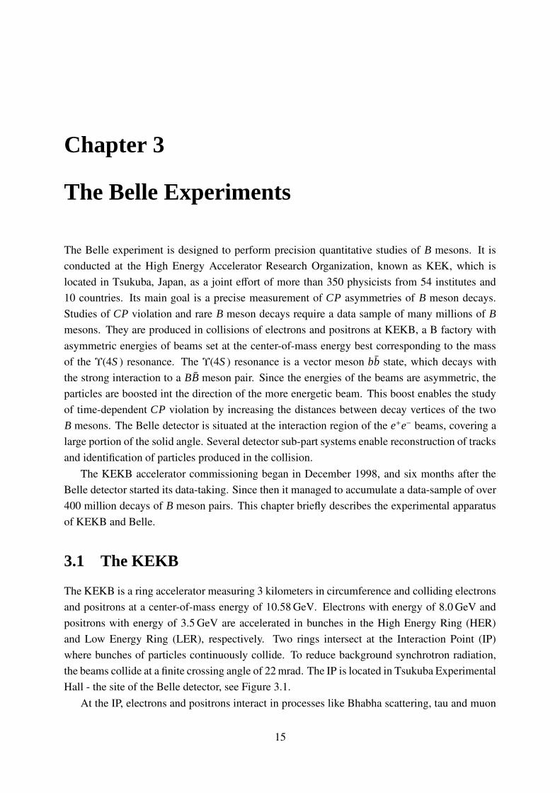
The KEKB is a ring accelerator measuring 3 kilometers in circumference and colliding electronsand positrons at a center-of-mass energy of 10.58 GeV. Electrons with energy of 8.0 GeV andpositrons with energy of 3.5 GeV are accelerated in bunches in the High Energy Ring (HER)and Low Energy Ring (LER), respectively. Two rings intersect at the Interaction Point (IP)where bunches of particles continuously collide. To reduce background synchrotron radiation,the beams collide at a finite crossing angle of 22 mrad. The IP is located in Tsukuba ExperimentalHall - the site of the Belle detector, see Figure 3.1.
At the IP, electrons and positrons interact in processes like Bhabha scattering, tau and muon
15
16 CHAPTER 3. THE BELLE EXPERIMENTS
Linac
TSUKUBA
OHO
FUJI
NIKKO
HER LER
HERLER
IP
RF
RF
RF
RF
e-e+
e+/e-
HER LER
RF
RF
WIGGLER
WIGGLER
(TRISTAN Accumulation Ring)
BYPASS
Figure 3.1: The KEKB Storage rings, LER and HER, with the IP located in Tsukuba Experimen-tal Hall.
pair production, quark pair production and two-photon events. Even though the center-of-massenergy is tailored for the Υ(4S ) resonance production as illustrated in Figure 3.2, only one Υ(4S )is produced in every e+e− interaction. The rate of the production, R is defined as the interactioncross section, σ, multiplied by the luminosity, L, measured in units of cm2 and cm−2s−1, respec-tively:
R = σL. (3.1)
The interaction cross section for the Υ(4S ) production at the center-of-mass energy 10.58 GeVis
σ(e+e− → Υ(4S )) = 1.1 nb, (3.2)
where the unit is barn, b ≡ 10−24cm2. The luminosity is a measure of the beam-colliding perfor-mance, and is given by
L = f · n · N1N2
A, (3.3)
where n bunches of N1 and N2 particles in opposing beams meet f times per second, and theoverlapping area of the beams is A.
The estimated maximum luminosity to be achieved in the proposal [31] was 1034 cm−2 sec−1,and has already been surpassed. A maximum luminosity of 1.7118 × 10 − 34cm−2 sec−1 wasachieved on November 15, 2006, and is currently the highest luminosity ever achieved by acollider. The measure of collected data is integrated luminosity (Lint):
Lint =
∫
Ldt. (3.4)
3.2. THE BELLE DETECTOR 17
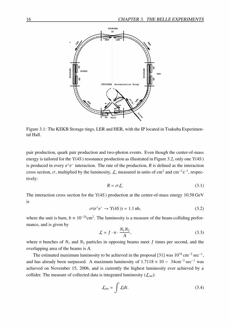
Figure 3.2: Cross section of e+e− → hadrons in a invariant mass range of 9.44 − 10.62 GeV/c2.
Taking the detector dead time into account, the Belle detector has accumulated the integratedluminosity of Lint = 710.254fb−1 on December 25, 2006.
3.2 The Belle Detector
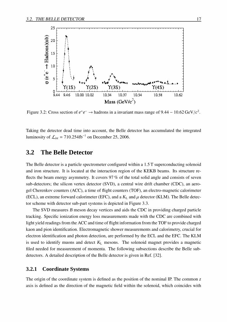
The Belle detector is a particle spectrometer configured within a 1.5 T superconducting solenoidand iron structure. It is located at the interaction region of the KEKB beams. Its structure re-flects the beam energy asymmetry. It covers 97 % of the total solid angle and consists of sevensub-detectors; the silicon vertex detector (SVD), a central wire drift chamber (CDC), an aero-gel Cherenkov counters (ACC), a time of flight counters (TOF), an electro-magnetic calorimeter(ECL), an extreme forward calorimeter (EFC), and a KL and µ detector (KLM). The Belle detec-tor scheme with detector sub-part systems is depicted in Figure 3.3.
The SVD measures B meson decay vertices and aids the CDC in providing charged particletracking. Specific ionization energy loss measurements made with the CDC are combined withlight yield readings from the ACC and time of flight information from the TOF to provide chargedkaon and pion identification. Electromagnetic shower measurements and calorimetry, crucial forelectron identification and photon detection, are performed by the ECL and the EFC. The KLMis used to identify muons and detect KL mesons. The solenoid magnet provides a magneticfiled needed for measurement of momenta. The following subsections describe the Belle sub-detectors. A detailed description of the Belle detector is given in Ref. [32].
3.2.1 Coordinate Systems
The origin of the coordinate system is defined as the position of the nominal IP. The common z
axis is defined as the direction of the magnetic field within the solenoid, which coincides with
18 CHAPTER 3. THE BELLE EXPERIMENTS
0 1 2 3 (m)
e- e+8.0 GeV 3.5 GeV
SVD
CDCCsI
KLMTOF
PID
150°
17°
EFC
Figure 3.3: Side view of the Belle detector.
the direction of the electron beam. The x and y axes are horizontal and vertical, respectively,and correspond to a right-handed coordinate system. The polar angle is measured relative to thepositive z axis. The azimuthal angle φ, laying in the x − y plane, is measured relative to thepositive x axis. The radius in the cylindrical coordinate system is defined as r =
√
x2 + y2.
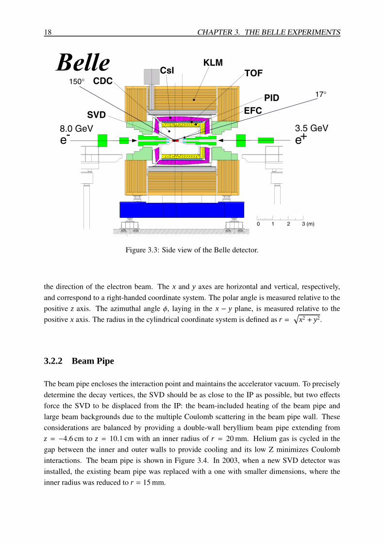
3.2.2 Beam Pipe
The beam pipe encloses the interaction point and maintains the accelerator vacuum. To preciselydetermine the decay vertices, the SVD should be as close to the IP as possible, but two effectsforce the SVD to be displaced from the IP: the beam-included heating of the beam pipe andlarge beam backgrounds due to the multiple Coulomb scattering in the beam pipe wall. Theseconsiderations are balanced by providing a double-wall beryllium beam pipe extending fromz = −4.6 cm to z = 10.1 cm with an inner radius of r = 20 mm. Helium gas is cycled in thegap between the inner and outer walls to provide cooling and its low Z minimizes Coulombinteractions. The beam pipe is shown in Figure 3.4. In 2003, when a new SVD detector wasinstalled, the existing beam pipe was replaced with a one with smaller dimensions, where theinner radius was reduced to r = 15 mm.
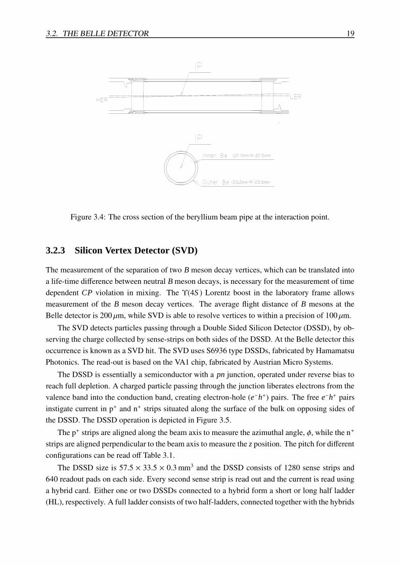
3.2. THE BELLE DETECTOR 19
Figure 3.4: The cross section of the beryllium beam pipe at the interaction point.
3.2.3 Silicon Vertex Detector (SVD)
The measurement of the separation of two B meson decay vertices, which can be translated intoa life-time difference between neutral B meson decays, is necessary for the measurement of timedependent CP violation in mixing. The Υ(4S ) Lorentz boost in the laboratory frame allowsmeasurement of the B meson decay vertices. The average flight distance of B mesons at theBelle detector is 200 µm, while SVD is able to resolve vertices to within a precision of 100 µm.
The SVD detects particles passing through a Double Sided Silicon Detector (DSSD), by ob-serving the charge collected by sense-strips on both sides of the DSSD. At the Belle detector thisoccurrence is known as a SVD hit. The SVD uses S6936 type DSSDs, fabricated by HamamatsuPhotonics. The read-out is based on the VA1 chip, fabricated by Austrian Micro Systems.
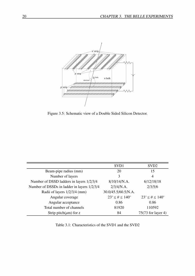
The DSSD is essentially a semiconductor with a pn junction, operated under reverse bias toreach full depletion. A charged particle passing through the junction liberates electrons from thevalence band into the conduction band, creating electron-hole (e−h+) pairs. The free e−h+ pairsinstigate current in p+ and n+ strips situated along the surface of the bulk on opposing sides ofthe DSSD. The DSSD operation is depicted in Figure 3.5.
The p+ strips are aligned along the beam axis to measure the azimuthal angle, φ, while the n+
strips are aligned perpendicular to the beam axis to measure the z position. The pitch for differentconfigurations can be read off Table 3.1.
The DSSD size is 57.5 × 33.5 × 0.3 mm3 and the DSSD consists of 1280 sense strips and640 readout pads on each side. Every second sense strip is read out and the current is read usinga hybrid card. Either one or two DSSDs connected to a hybrid form a short or long half ladder(HL), respectively. A full ladder consists of two half-ladders, connected together with the hybrids
20 CHAPTER 3. THE BELLE EXPERIMENTS
n bulk
strip+n
strip+p
electron
hole
stopp-
Figure 3.5: Schematic view of a Double Sided Silicon Detector.
SVD1 SVD2Beam-pipe radius (mm) 20 15
Number of layers 3 4Number of DSSD ladders in layers 1/2/3/4 8/10/14/N.A. 6/12/18/18
Number of DSSDs in ladder in layers 1/2/3/4 2/3/4/N.A. 2/3/5/6Radii of layers 1/2/3/4 (mm) 30.0/45.5/60.5/N.A.
Angular coverage 23◦≤ θ ≤ 140◦ 23◦≤ θ ≤ 140◦Angular acceptance 0.86 0.86
Total number of channels 81920 110592Strip pitch(µm) for z 84 75(73 for layer 4)
Table 3.1: Characteristics of the SVD1 and the SVD2
3.2. THE BELLE DETECTOR 21
at the ends. Full ladders are arranged in cylindrical layers.Two SVD configurations were used in the period of the data taking, the SVD1 (1998-2003)
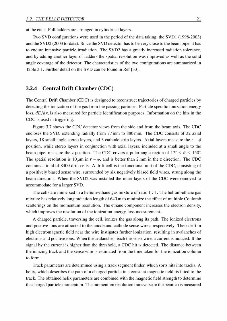
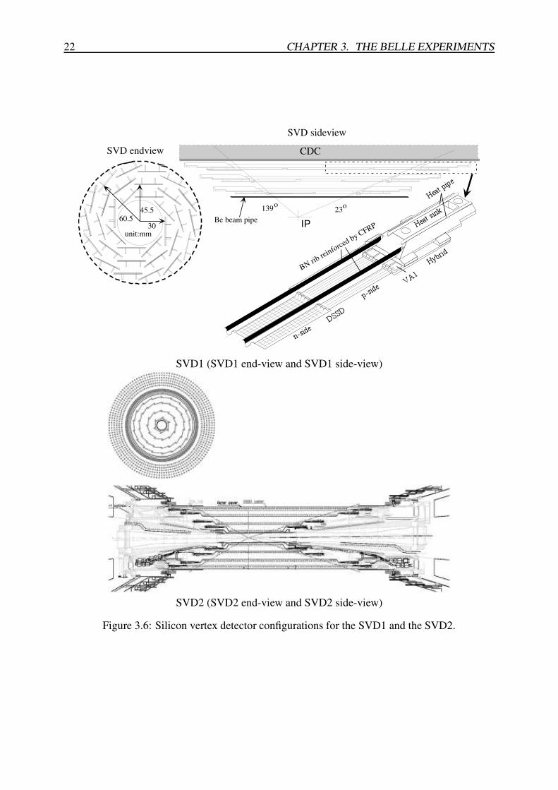
and the SVD2 (2003 to-date). Since the SVD detector has to be very close to the beam pipe, it hasto endure intensive particle irradiation. The SVD2 has a greatly increased radiation tolerance,and by adding another layer of ladders the spatial resolution was improved as well as the solidangle coverage of the detector. The characteristics of the two configurations are summarized inTable 3.1. Further detail on the SVD can be found in Ref [33].
3.2.4 Central Drift Chamber (CDC)
The Central Drift Chamber (CDC) is designed to reconstruct trajectories of charged particles bydetecting the ionization of the gas from the passing particles. Particle specific ionization energyloss, dE/dx, is also measured for particle identification purposes. Information on the hits in theCDC is used in triggering.
Figure 3.7 shows the CDC detector views from the side and from the beam axis. The CDCencloses the SVD, extending radially from 77 mm to 880 mm. The CDC consists of 32 axiallayers, 18 small angle stereo layers, and 3 cathode strip layers. Axial layers measure the r − φposition, while stereo layers in conjunction with axial layers, included at a small angle to thebeam pipe, measure the z position. The CDC covers a polar angle region of 17◦ ≤ θ ≤ 150◦.The spatial resolution is 10 µm in r − φ, and is better than 2 mm in the z direction. The CDCcontains a total of 8400 drift cells. A drift cell is the functional unit of the CDC, consisting ofa positively biased sense wire, surrounded by six negatively biased field wires, strung along thebeam direction. When the SVD2 was installed the inner layers of the CDC were removed toaccommodate for a larger SVD.
The cells are immersed in a helium-ethane gas mixture of ratio 1 : 1. The helium-ethane gasmixture has relatively long radiation length of 640 m to minimize the effect of multiple Coulombscatterings on the momentum resolution. The ethane component increases the electron density,which improves the resolution of the ionization-energy-loss measurement.
A charged particle, traversing the cell, ionizes the gas along its path. The ionized electronsand positive ions are attracted to the anode and cathode sense wires, respectively. Their drift inhigh electromagnetic field near the wire instigates further ionization, resulting in avalanches ofelectrons and positive ions. When the avalanches reach the sense wire, a current is induced. If thesignal by the current is higher than the threshold, a CDC hit is detected. The distance betweenthe ionizing track and the sense wire is estimated from the time taken for the ionization columnto form.
Track parameters are determined using a track segment finder, which sorts hits into tracks. Ahelix, which describes the path of a charged particle in a constant magnetic field, is fitted to thetrack. The obtained helix parameters are combined with the magnetic field strength to determinethe charged particle momentum. The momentum resolution transverse to the beam axis measured
22 CHAPTER 3. THE BELLE EXPERIMENTS
CDC
23o139o
IPBe beam pipe30
45.560.5
unit:mm
SVD sideview
SVD endview
BN rib reinforced by CFRP
SVD1 (SVD1 end-view and SVD1 side-view)
SVD2 (SVD2 end-view and SVD2 side-view)
Figure 3.6: Silicon vertex detector configurations for the SVD1 and the SVD2.
3.2. THE BELLE DETECTOR 23
747.0
790.0 1589.6
880
702.2 1501.8
BELLE Central Drift Chamber
5
10
r
2204
294
83
Cathode part
Inner part
Main part
ForwardBackward
eeInteraction Point
17°150°
y
x100mm
y
x100mm
- +
Figure 3.7: The Central Drift Chamber (CDC): side-view (left) and end-view (right).
11.25°
Layer
unit: mm
5.00103.00
Layer
83.00
Layer
2
1
45°
Field wire11.25°
Sense wire
0
Field Wire Al 126µmφSense Wire Au plated W 30µmφ
BELLE Central Drift Chamber
16m
m
17mm
Figure 3.8: Cross-sectional view of cell structure of the CDC. Cathode strips are also drawn byhatches in the left figure.
24 CHAPTER 3. THE BELLE EXPERIMENTS
from cosmic ray data, isσpT
pT=
√
(0.20pT)2 + (0.29/β)2 %, (3.5)
where pT is in units of GeV/c and β is the particle velocity divided by the speed of light. Fig-ure 3.9 shows the resolution of the transverse momentum.
2 (P
t
- P
t
)/(P
t
+P
t
)] (
%)
0
0.4
0.8
1.2
1.6
2
0 1 2 3 4 5Pt ( Gev/c )
Fit
( 0.201 ± 0.003 ) % Pt ⊕ ( 0.290 ± 0.006 ) %
dow
n
up
do
wn
up
σ[ √
Figure 3.9: Resolution of the transverse momentum of the CDC.
Particle energy loss in a drift cell due to ionization, dE/dx, is determined from a hit ampli-tude recorded on a sense wire. Since the energy loss depends on a particle velocity at a givenmomentum, dE/dx distributions differs for different particle masses, as shown in Figure 3.10.The ionization energy loss is measured for each CDC hit and measurements along the trajectoryare combined to calculate the truncated mean, 〈dE/dx〉, of the track.
The 〈dE/dx〉 resolution, measured on a sample of pions from KS decays, is 7.8 %. The CDCcan be used to distinguish pions from kaons of momenta up to 0.8 GeV/c with a 3σ separation.A detailed description of CDC is presented in Ref [34].
3.2.5 Aerogel Cherenkov Counter (ACC)
The silica Aerogel Cherenkov Counter (ACC) plays a crucial role in discriminating charged pionsfrom kaons. When a particle travels faster than the speed of light in that medium, it will emitCherenkov light. The emitted light appears in the form of a coherent wavefront at a fixed anglewith respect to the trajectory.
To emit Cherenkov light, the particle velocity has to be grater than the threshold value:
β > βthreshold =1n
(3.6)
where n is the refractive index of the medium. Threshold Cherenkov counters exploit the fact thatonly particles with velocity above βthreshold can emit Cherenkov photons. Since the momentum
3.2. THE BELLE DETECTOR 25
0.5
1
1.5
2
2.5
3
3.5
4
-1.5 -1 -0.5 0 0.5 1
dE/dx vs log10(p)log10(p)
dE
/dx
PK
e
π
Figure 3.10: Truncated mean of dE/dx versus momentum The points are measurements takenduring accelerator operations, and the lines are the expected distributions of each particle type.p is measured in GeV/c.
is measured by the other sub-detectors, the particles can be identified be observing whetherCherenkov photons have been detected or not.
K/π discrimination can be achieved by selecting media with appropriate refractive indicesto cover typical momenta. The ACC augments the other detector subsystems by performingexcellent K/π separation for momenta between 2.5 and 3.5 GeV/c, and is also able to provideuseful information for momenta as low as 1.5 GeV/c and as high as 4.0 GeV/c.
The ACC is divided into barrel and forward end-cap regions and is shown in Figure 3.11. Itspans a polar angle region of 17◦ ≤ θ ≤ 127◦. The barrel ACC contains 960 counter modules,segmented into 60 cells in the φ direction. The forward end-cap ACC contains 228 countermodules, arranged into 5 concentric layers. Depending on the polar angle, the refractive indexof the aerogel tiles ranges from n = 1.01 to 1.03. One of concerns when using aerogel is thatits transparency is greatly reduced with age due to its hydrophilic property. A special aerogelproduction procedure has been developed so that it is possible to produce hydrophobic aerogel.
Cherenkov photons are detected by either one or two fine mesh-type photo-multiplier tubes(FM-PMT), which are attached to each counter. The ACC detector is positioned within a strongmagnetic field, which drastically reduces the gain and the collection efficiency of photoelectrons.By using a fine FM-PMT with 19 dynodes, a high gain of 108 is maintained even in the strongmagnetic field. Three different sizes of FM-PMT with radii of 1, 1.25 and 1.5 inches are used.The choice is dependent on the refractive index to keep the constant photon yield, since a lowerrefractive index results in a lower yield, barrel and end-cap modules are depicted in Figure 3.12.
The pulse height for each FM-PMT has been calibrated using µ-pair events. The average
26 CHAPTER 3. THE BELLE EXPERIMENTS
B (1.5Tesla)
BELLE Aerogel Cherenkov Counter
3" FM-PMT2.5" FM-PMT
2" FM-PMT
17°
127 ° 34 °
Endcap ACC
885
R(BACC/inner)
1145
R(EACC/outer)
1622 (BACC)
1670 (EACC/inside)
1950 (EACC/outside)
854 (BACC)
1165
R(BACC/outer)
0.0m1.0m2.0m3.0m 2.5m 1.5m 0.5m
n=1.02860mod.
n=1.020240mod.
n=1.015240mod.
n=1.01360mod.
n=1.010360mod.
Barrel ACC
n=1.030228mod.
TOF/TSC
CDC
Figure 3.11: The configuration of the Aerogel Cherenkov Counter.
Aerogel
Goretex
Finemesh PMT
Finemesh PMT
120 mm
120 mm
Aluminum container (0.2mm thick)
a) Barrel ACC Module
Aerogel
Goretex Reflector
CFRP(0.5mm thick)
Air light guide
FM-Phototube
Base & Amplifier
(CFRP)
b) Endcap ACC Module
Figure 3.12: Schematic drawing of a typical ACC counter module : (a) barrel and (b) end-capACC.
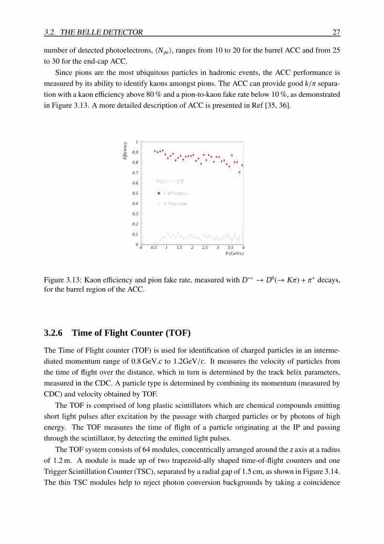
3.2. THE BELLE DETECTOR 27
number of detected photoelectrons, 〈Npe〉, ranges from 10 to 20 for the barrel ACC and from 25to 30 for the end-cap ACC.
Since pions are the most ubiquitous particles in hadronic events, the ACC performance ismeasured by its ability to identify kaons amongst pions. The ACC can provide good k/π separa-tion with a kaon efficiency above 80 % and a pion-to-kaon fake rate below 10 %, as demonstratedin Figure 3.13. A more detailed description of ACC is presented in Ref [35, 36].
0
0.1
0.2
0.3
0.4
0.5
0.6
0.7
0.8
0.9
1
0 0.5 1 1.5 2 2.5 3 3.5 4P (GeV/c)
Eff
icie
ncy
Figure 3.13: Kaon efficiency and pion fake rate, measured with D∗+ → D0(→ Kπ) + π+ decays,for the barrel region of the ACC.
3.2.6 Time of Flight Counter (TOF)
The Time of Flight counter (TOF) is used for identification of charged particles in an interme-diated momentum range of 0.8 GeV.c to 1.2GeV/c. It measures the velocity of particles fromthe time of flight over the distance, which in turn is determined by the track helix parameters,measured in the CDC. A particle type is determined by combining its momentum (measured byCDC) and velocity obtained by TOF.
The TOF is comprised of long plastic scintillators which are chemical compounds emittingshort light pulses after excitation by the passage with charged particles or by photons of highenergy. The TOF measures the time of flight of a particle originating at the IP and passingthrough the scintillator, by detecting the emitted light pulses.
The TOF system consists of 64 modules, concentrically arranged around the z axis at a radiusof 1.2 m. A module is made up of two trapezoid-ally shaped time-of-flight counters and oneTrigger Scintillation Counter (TSC), separated by a radial gap of 1.5 cm, as shown in Figure 3.14.The thin TSC modules help to reject photon conversion backgrounds by taking a coincidence
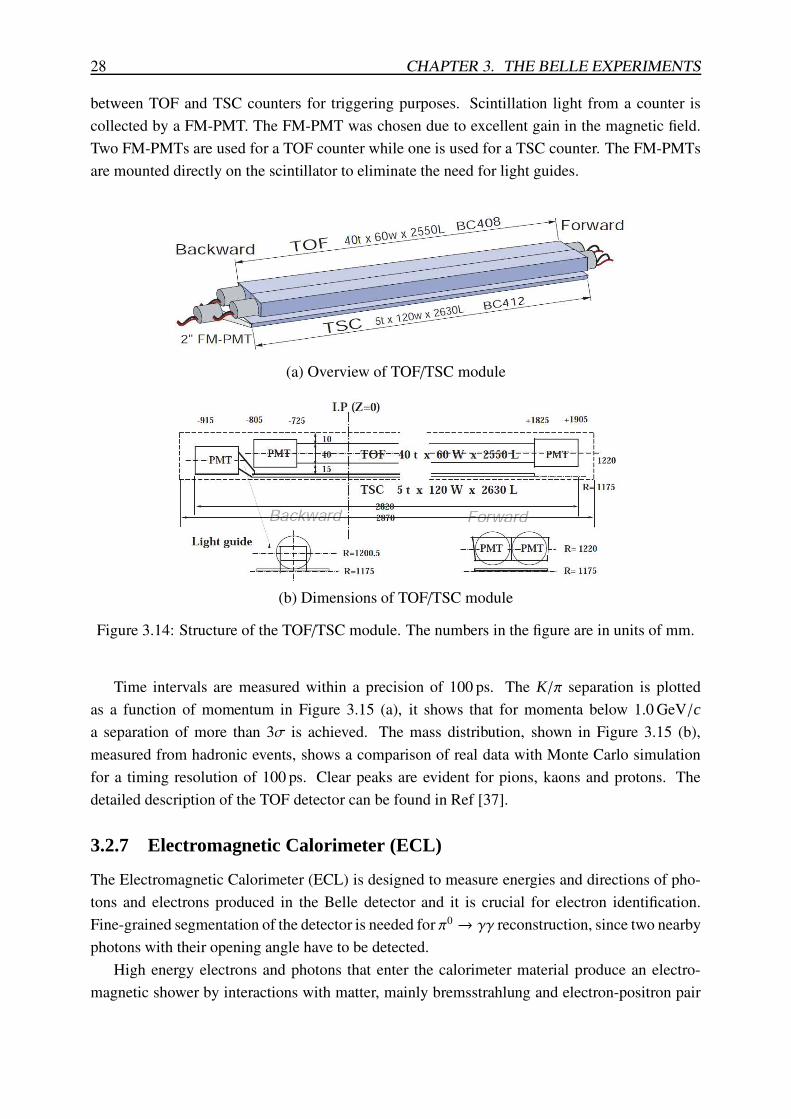
28 CHAPTER 3. THE BELLE EXPERIMENTS
between TOF and TSC counters for triggering purposes. Scintillation light from a counter iscollected by a FM-PMT. The FM-PMT was chosen due to excellent gain in the magnetic field.Two FM-PMTs are used for a TOF counter while one is used for a TSC counter. The FM-PMTsare mounted directly on the scintillator to eliminate the need for light guides.
(a) Overview of TOF/TSC module
(b) Dimensions of TOF/TSC module
Figure 3.14: Structure of the TOF/TSC module. The numbers in the figure are in units of mm.
Time intervals are measured within a precision of 100 ps. The K/π separation is plottedas a function of momentum in Figure 3.15 (a), it shows that for momenta below 1.0 GeV/ca separation of more than 3σ is achieved. The mass distribution, shown in Figure 3.15 (b),measured from hadronic events, shows a comparison of real data with Monte Carlo simulationfor a timing resolution of 100 ps. Clear peaks are evident for pions, kaons and protons. Thedetailed description of the TOF detector can be found in Ref [37].
3.2.7 Electromagnetic Calorimeter (ECL)
The Electromagnetic Calorimeter (ECL) is designed to measure energies and directions of pho-tons and electrons produced in the Belle detector and it is crucial for electron identification.Fine-grained segmentation of the detector is needed for π0 → γγ reconstruction, since two nearbyphotons with their opening angle have to be detected.
High energy electrons and photons that enter the calorimeter material produce an electro-magnetic shower by interactions with matter, mainly bremsstrahlung and electron-positron pair
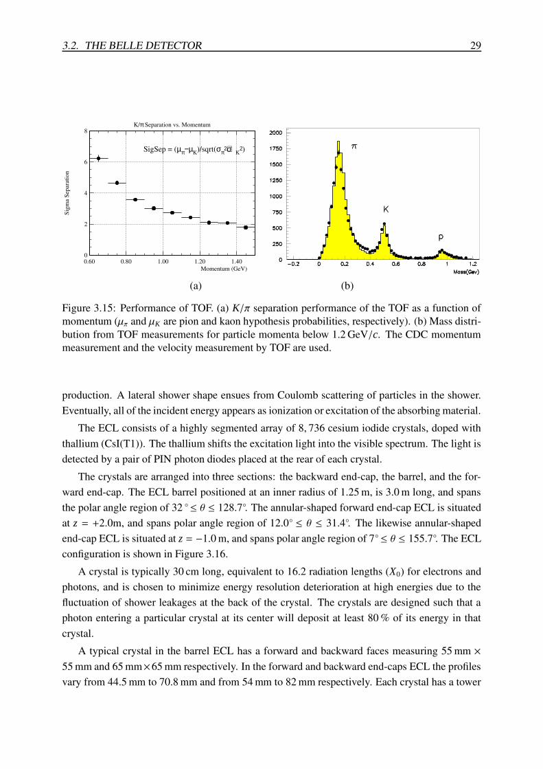
3.2. THE BELLE DETECTOR 29
K/π Separation vs. Momentum
0.60 0.80 1.00 1.20 1.40Momentum (GeV)
0
2
4
6
8
Sigm
a Se
para
tion
SigSep = (µπ−µK)/sqrt(σπ2+σK
2)
(a) (b)
Figure 3.15: Performance of TOF. (a) K/π separation performance of the TOF as a function ofmomentum (µπ and µK are pion and kaon hypothesis probabilities, respectively). (b) Mass distri-bution from TOF measurements for particle momenta below 1.2 GeV/c. The CDC momentummeasurement and the velocity measurement by TOF are used.
production. A lateral shower shape ensues from Coulomb scattering of particles in the shower.Eventually, all of the incident energy appears as ionization or excitation of the absorbing material.
The ECL consists of a highly segmented array of 8, 736 cesium iodide crystals, doped withthallium (CsI(T1)). The thallium shifts the excitation light into the visible spectrum. The light isdetected by a pair of PIN photon diodes placed at the rear of each crystal.
The crystals are arranged into three sections: the backward end-cap, the barrel, and the for-ward end-cap. The ECL barrel positioned at an inner radius of 1.25 m, is 3.0 m long, and spansthe polar angle region of 32 ◦≤ θ ≤ 128.7◦. The annular-shaped forward end-cap ECL is situatedat z = +2.0m, and spans polar angle region of 12.0◦ ≤ θ ≤ 31.4◦. The likewise annular-shapedend-cap ECL is situated at z = −1.0 m, and spans polar angle region of 7◦≤ θ ≤ 155.7◦. The ECLconfiguration is shown in Figure 3.16.
A crystal is typically 30 cm long, equivalent to 16.2 radiation lengths (X0) for electrons andphotons, and is chosen to minimize energy resolution deterioration at high energies due to thefluctuation of shower leakages at the back of the crystal. The crystals are designed such that aphoton entering a particular crystal at its center will deposit at least 80 % of its energy in thatcrystal.
A typical crystal in the barrel ECL has a forward and backward faces measuring 55 mm ×55 mm and 65 mm×65 mm respectively. In the forward and backward end-caps ECL the profilesvary from 44.5 mm to 70.8 mm and from 54 mm to 82 mm respectively. Each crystal has a tower
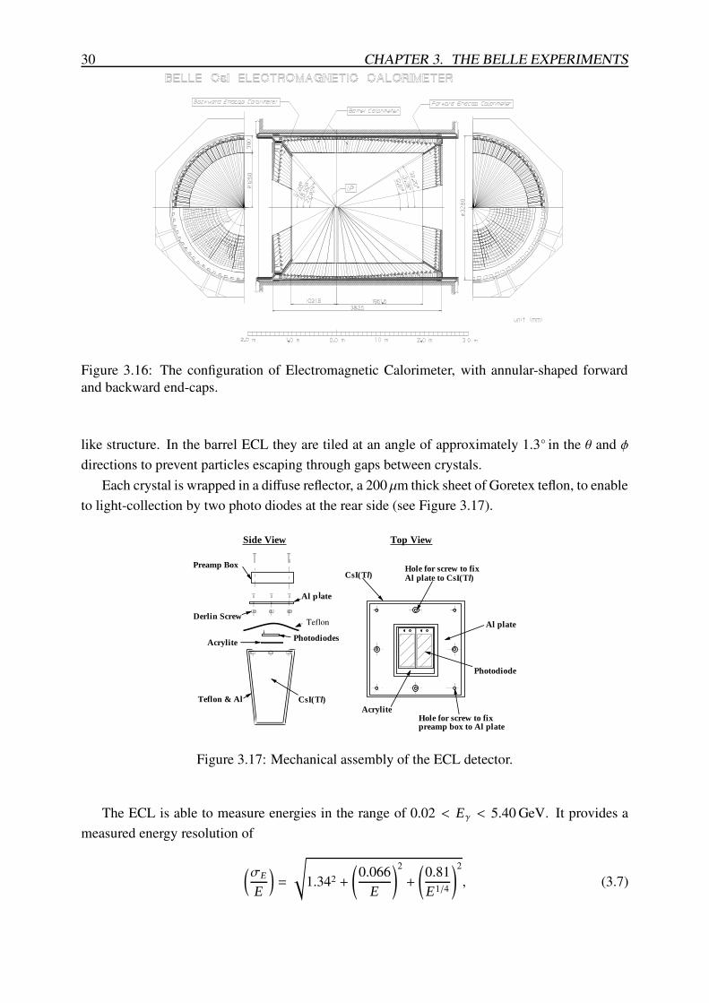
30 CHAPTER 3. THE BELLE EXPERIMENTS
Figure 3.16: The configuration of Electromagnetic Calorimeter, with annular-shaped forwardand backward end-caps.
like structure. In the barrel ECL they are tiled at an angle of approximately 1.3◦ in the θ and φdirections to prevent particles escaping through gaps between crystals.
Each crystal is wrapped in a diffuse reflector, a 200 µm thick sheet of Goretex teflon, to enableto light-collection by two photo diodes at the rear side (see Figure 3.17).
CsI(Tl)
l
Teflon & Al
Acrylite Photodiodes
Al p ate
Derlin Screw
Preamp Box
Photodiode
CsI(Tl)
Al plate
Acrylite
Hole for screw to fixAl plate to CsI(Tl)
Hole for screw to fixpreamp box to Al plate
Top ViewSide View
Teflon
Figure 3.17: Mechanical assembly of the ECL detector.
The ECL is able to measure energies in the range of 0.02 < Eγ < 5.40 GeV. It provides ameasured energy resolution of
(
σE
E
)
=
√
1.342 +
(
0.066E
)2
+
(
0.81E1/4
)2
, (3.7)
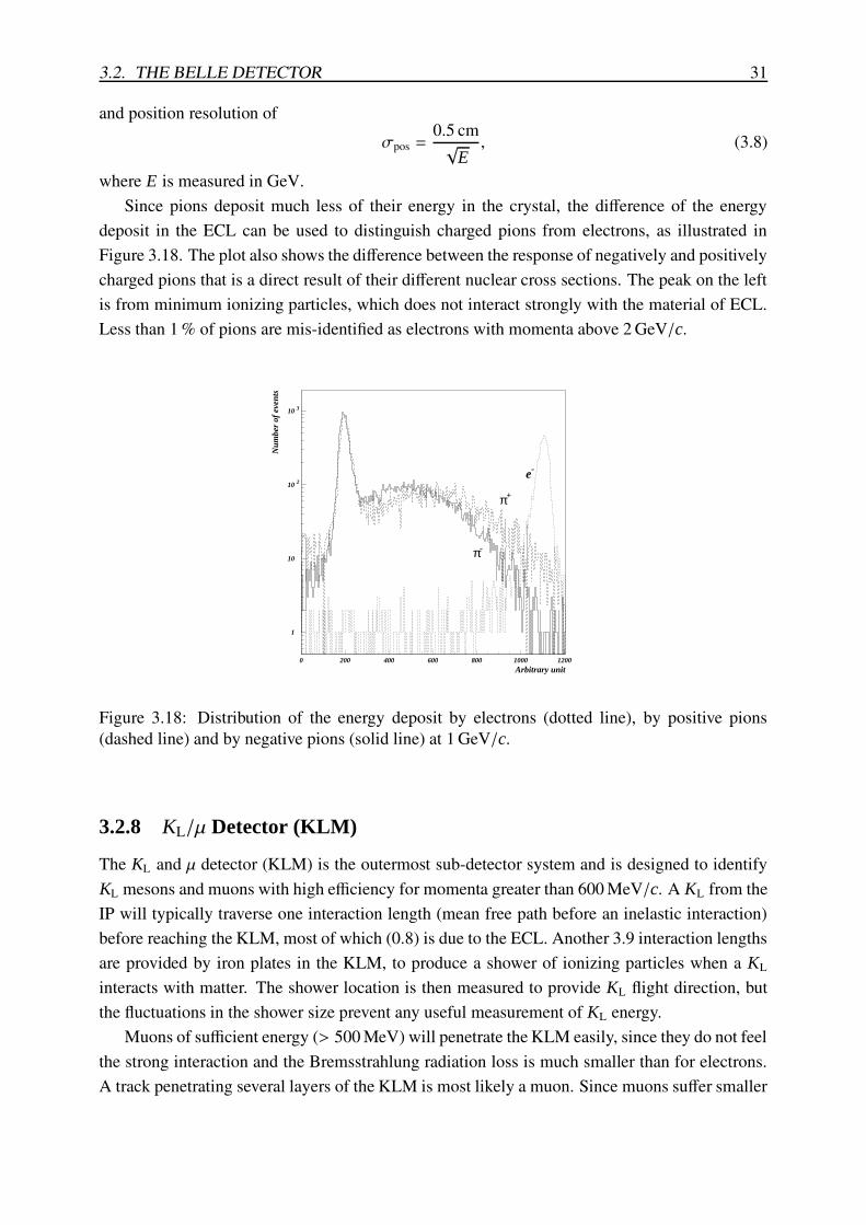
3.2. THE BELLE DETECTOR 31
and position resolution ofσpos =
0.5 cm√
E, (3.8)
where E is measured in GeV.Since pions deposit much less of their energy in the crystal, the difference of the energy
deposit in the ECL can be used to distinguish charged pions from electrons, as illustrated inFigure 3.18. The plot also shows the difference between the response of negatively and positivelycharged pions that is a direct result of their different nuclear cross sections. The peak on the leftis from minimum ionizing particles, which does not interact strongly with the material of ECL.Less than 1 % of pions are mis-identified as electrons with momenta above 2 GeV/c.
1
10
10 2
10 3
0 200 400 600 800 1000 1200Arbitrary unit
Num
ber
of e
vent
s
π-
π+
e-
Figure 3.18: Distribution of the energy deposit by electrons (dotted line), by positive pions(dashed line) and by negative pions (solid line) at 1 GeV/c.
3.2.8 KL/µ Detector (KLM)
The KL and µ detector (KLM) is the outermost sub-detector system and is designed to identifyKL mesons and muons with high efficiency for momenta greater than 600 MeV/c. A KL from theIP will typically traverse one interaction length (mean free path before an inelastic interaction)before reaching the KLM, most of which (0.8) is due to the ECL. Another 3.9 interaction lengthsare provided by iron plates in the KLM, to produce a shower of ionizing particles when a KL
interacts with matter. The shower location is then measured to provide KL flight direction, butthe fluctuations in the shower size prevent any useful measurement of KL energy.
Muons of sufficient energy (> 500 MeV) will penetrate the KLM easily, since they do not feelthe strong interaction and the Bremsstrahlung radiation loss is much smaller than for electrons.A track penetrating several layers of the KLM is most likely a muon. Since muons suffer smaller
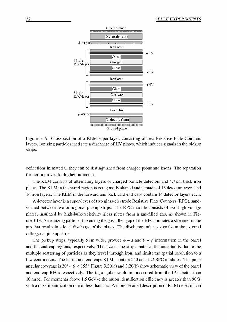
32 CHAPTER 3. THE BELLE EXPERIMENTS
Figure 3.19: Cross section of a KLM super-layer, consisting of two Resistive Plate Counterslayers. Ionizing particles instigate a discharge of HV plates, which induces signals in the pickupstrips.
deflections in material, they can be distinguished from charged pions and kaons. The separationfurther improves for higher momenta.
The KLM consists of alternating layers of charged-particle detectors and 4.7 cm thick ironplates. The KLM in the barrel region is octagonally shaped and is made of 15 detector layers and14 iron layers. The KLM in the forward and backward end-caps contain 14 detector layers each.
A detector layer is a super-layer of two glass-electrode Resistive Plate Counters (RPC), sand-wiched between two orthogonal pickup strips. The RPC module consists of two high-voltageplates, insulated by high-bulk-resistivity glass plates from a gas-filled gap, as shown in Fig-ure 3.19. An ionizing particle, traversing the gas-filled gap of the RPC, initiates a streamer in thegas that results in a local discharge of the plates. The discharge induces signals on the externalorthogonal pickup strips.
The pickup strips, typically 5 cm wide, provide φ − z and θ − φ information in the barreland the end-cap regions, respectively. The size of the strips matches the uncertainty due to themultiple scattering of particles as they travel through iron, and limits the spatial resolution to afew centimeters. The barrel and end-caps KLMs contain 240 and 122 RPC modules. The polarangular coverage is 20◦< θ < 155◦. Figure 3.20(a) and 3.20(b) show schematic view of the barreland end-cap RPCs respectively. The KL angular resolution measured from the IP is better than10 mrad. For momenta above 1.5 GeV/c the muon identification efficiency is greater than 90 %with a miss-identification rate of less than 5 %. A more detailed description of KLM detector can
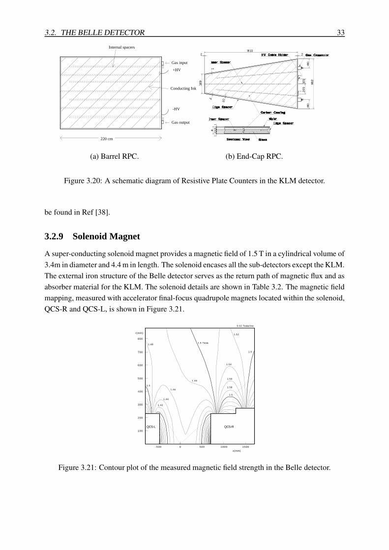
3.2. THE BELLE DETECTOR 33
Gas output
220 cm
+HV
-HV
Internal spacers
Conducting Ink
Gas input
(a) Barrel RPC. (b) End-Cap RPC.
Figure 3.20: A schematic diagram of Resistive Plate Counters in the KLM detector.
be found in Ref [38].
3.2.9 Solenoid Magnet
A super-conducting solenoid magnet provides a magnetic field of 1.5 T in a cylindrical volume of3.4m in diameter and 4.4 m in length. The solenoid encases all the sub-detectors except the KLM.The external iron structure of the Belle detector serves as the return path of magnetic flux and asabsorber material for the KLM. The solenoid details are shown in Table 3.2. The magnetic fieldmapping, measured with accelerator final-focus quadrupole magnets located within the solenoid,QCS-R and QCS-L, is shown in Figure 3.21.
0-500 500 1000 1500
1.5 Tesla
100
200
300
400
500
600
700
800
z(mm)
r(mm)
1.5
1.5
1.46
1.48
1.54
1.52
1.56
QCS-RQCS-L
1.44
1.42
1.48
1.58
1.6
0.02 Tesla/ line
Figure 3.21: Contour plot of the measured magnetic field strength in the Belle detector.
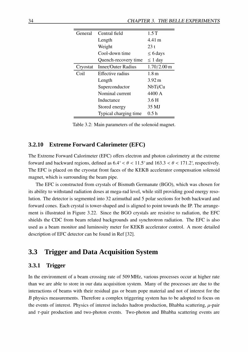
34 CHAPTER 3. THE BELLE EXPERIMENTS
General Central field 1.5 TLength 4.41 mWeight 23 tCool-down time ≤ 6 daysQuench-recovery time ≤ 1 day
Cryostat Inner/Outer Radius 1.70/2.00 mCoil Effective radius 1.8 m
Length 3.92 mSuperconductor NbTi/CuNominal current 4400 AInductance 3.6 HStored energy 35 MJTypical charging time 0.5 h
Table 3.2: Main parameters of the solenoid magnet.
3.2.10 Extreme Forward Calorimeter (EFC)
The Extreme Forward Calorimeter (EFC) offers electron and photon calorimetry at the extremeforward and backward regions, defined as 6.4◦< θ < 11.5◦ and 163.3 < θ < 171.2◦, respectively.The EFC is placed on the cryostat front faces of the KEKB accelerator compensation solenoidmagnet, which is surrounding the beam pipe.
The EFC is constructed from crystals of Bismuth Germanate (BGO), which was chosen forits ability to withstand radiation doses at mega-rad level, while still providing good energy reso-lution. The detector is segmented into 32 azimuthal and 5 polar sections for both backward andforward cones. Each crystal is tower-shaped and is aligned to point towards the IP. The arrange-ment is illustrated in Figure 3.22. Since the BGO crystals are resistive to radiation, the EFCshields the CDC from beam related backgrounds and synchrotron radiation. The EFC is alsoused as a beam monitor and luminosity meter for KEKB accelerator control. A more detaileddescription of EFC detector can be found in Ref [32].
3.3 Trigger and Data Acquisition System
3.3.1 Trigger
In the environment of a beam crossing rate of 509 MHz, various processes occur at higher ratethan we are able to store in our data acquisition system. Many of the processes are due to theinteractions of beams with their residual gas or beam pope material and not of interest for theB physics measurements. Therefore a complex triggering system has to be adopted to focus onthe events of interest. Physics of interest includes hadron production, Bhabha scattering, µ-pairand τ-pair production and two-photon events. Two-photon and Bhabha scattering events are
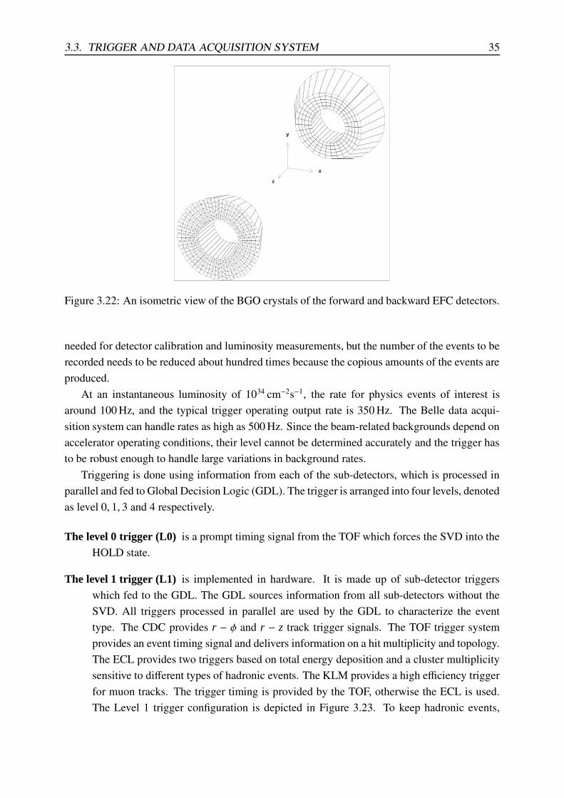
3.3. TRIGGER AND DATA ACQUISITION SYSTEM 35
x
y
z
Figure 3.22: An isometric view of the BGO crystals of the forward and backward EFC detectors.
needed for detector calibration and luminosity measurements, but the number of the events to berecorded needs to be reduced about hundred times because the copious amounts of the events areproduced.
At an instantaneous luminosity of 1034 cm−2s−1, the rate for physics events of interest isaround 100 Hz, and the typical trigger operating output rate is 350 Hz. The Belle data acqui-sition system can handle rates as high as 500 Hz. Since the beam-related backgrounds depend onaccelerator operating conditions, their level cannot be determined accurately and the trigger hasto be robust enough to handle large variations in background rates.
Triggering is done using information from each of the sub-detectors, which is processed inparallel and fed to Global Decision Logic (GDL). The trigger is arranged into four levels, denotedas level 0, 1, 3 and 4 respectively.
The level 0 trigger (L0) is a prompt timing signal from the TOF which forces the SVD into theHOLD state.
The level 1 trigger (L1) is implemented in hardware. It is made up of sub-detector triggerswhich fed to the GDL. The GDL sources information from all sub-detectors without theSVD. All triggers processed in parallel are used by the GDL to characterize the eventtype. The CDC provides r − φ and r − z track trigger signals. The TOF trigger systemprovides an event timing signal and delivers information on a hit multiplicity and topology.The ECL provides two triggers based on total energy deposition and a cluster multiplicitysensitive to different types of hadronic events. The KLM provides a high efficiency triggerfor muon tracks. The trigger timing is provided by the TOF, otherwise the ECL is used.The Level 1 trigger configuration is depicted in Figure 3.23. To keep hadronic events,

36 CHAPTER 3. THE BELLE EXPERIMENTS
the GDL typically relies on three main trigger classes; multi-tracks from the CDC, totalenergy deposition and isolated cluster counts from the ECL. Each provides more than96 % efficiency for hadronic events individually, and 99.5 % efficiency is achieved by thecombination.
The level 3 trigger (L3) is implemented in software in an online computer farm. Using an ultra-fast track finder it requires at least one track with an impact parameter in z less than 5.0 cmand the total energy deposit in the ECL to be greater than 3.0 GeV. The trigger reduces theevent rate by 50 − 60 % while retaining 99 % of events of interest.
The level 4 trigger (L4) is implemented in software and performed offline on a computer farmbefore full event reconstruction. Its purpose is to reduce the amount of data that goes tothe full event reconstruction, and its algorithms are optimized for speed. The conditionsthat activate the trigger are:
• Events are accepted in case that those are tagged by the hardware L1 trigger preselec-tion to be used for luminosity measurement, detector calibration or beam-backgroundstudies.
• A total ECL energy deposit is less than 4 GeV/c2 by the fast cluster-finder routine. Toreduce background from cosmic rays, this is vetoed by events with coincident KLMand ECL hits as encoded in L1 trigger information.
• At least one track with r and |z| distances to IP is less than 1.0 cm and 4.0 cm, respec-tively and pT is higher than 300 MeV/c.
• For monitoring purposes, 1 % of non-triggered events are kept.
The criteria retain hadronic events with an efficiency of 99.8 % while reducing the totalevent trigger rate by around 73 %.
3.3.2 Data Acquisition System
The Data Acquisition (DAQ) system manages and stores the data collected at the Belle detector.It is able to process data at the trigger rate of 500 Hz, while having a dead-time of less than 10 %.The system is shown in Figure 3.24. The data from each sub-detector are processed in sevenparallel sub-systems, and transformed into full event records by the Event Builder. The full eventrecords are sent to the online farm, where the data are filtered through the L3 software triggerand transformed into the offline event format suitable for offline analysis. A single event size isapproximately 30 kBytes of disk space, which translates into a data flow of 15 MBytes/s. Thedata is sent to the tape library at the computer center 2 km away, where it are written to tapes bya high-speed tape drive. The data monitoring system analyzes events at a rate of approximately20 Hz of events and can be plugged into the data stream without affecting it.
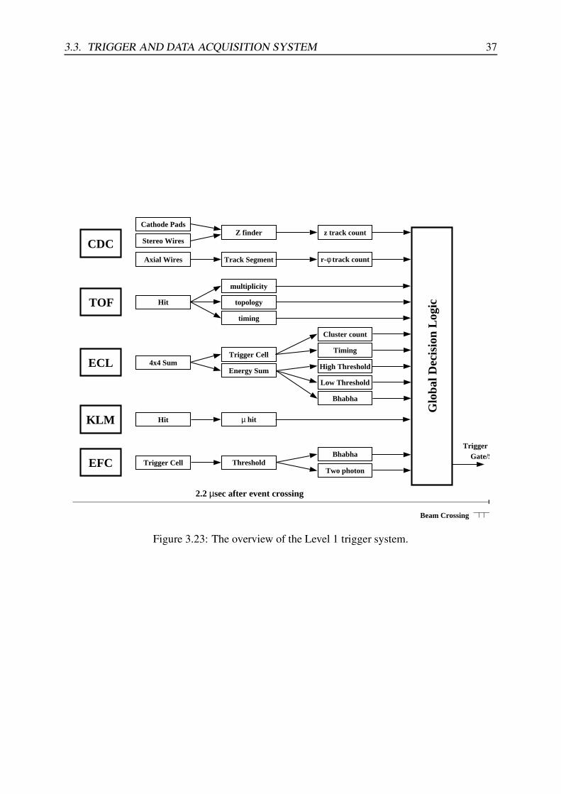
3.3. TRIGGER AND DATA ACQUISITION SYSTEM 37
Glo
bal D
ecis
ion
Log
ic
CDC
EFC
TOF
KLM
ECL
Cathode Pads
Stereo Wires
Axial Wires Track Segment
z track count
r-φ track count
Z finder
High Threshold
Trigger Cell ThresholdBhabha
Two photon
Hit
multiplicity
topology
timing
Hit µ hit
4x4 SumTrigger Cell
Energy Sum
Cluster count
Timing
Low Threshold
Bhabha
Trigger Signal Gate/Stop
Beam Crossing
2.2 µsec after event crossing
Figure 3.23: The overview of the Level 1 trigger system.
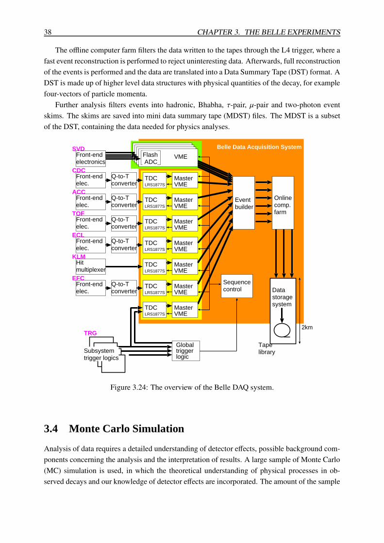
38 CHAPTER 3. THE BELLE EXPERIMENTS
The offline computer farm filters the data written to the tapes through the L4 trigger, where afast event reconstruction is performed to reject uninteresting data. Afterwards, full reconstructionof the events is performed and the data are translated into a Data Summary Tape (DST) format. ADST is made up of higher level data structures with physical quantities of the decay, for examplefour-vectors of particle momenta.
Further analysis filters events into hadronic, Bhabha, τ-pair, µ-pair and two-photon eventskims. The skims are saved into mini data summary tape (MDST) files. The MDST is a subsetof the DST, containing the data needed for physics analyses.
Front-endelec.
Q-to-Tconverter
MasterVME
MasterVME
MasterVME
Front-endelec.
Q-to-Tconverter
MasterVME
Front-endelec.
Q-to-Tconverter
MasterVME
MasterVME
Front-endelec.
Q-to-Tconverter
Eventbuilder
Onlinecomp.farm
Datastoragesystem
Tapelibrary
Sequencecontrol
Globaltriggerlogic
TDCLRS1877S
TDCLRS1877S
TDCLRS1877S
TDCLRS1877S
TDCLRS1877S
TDCLRS1877S
2km
SVD
CDC
ACC
TOF
KLM
ECL
VMEFlash ADC
Front-endelectronics
Subsystemtrigger logics
MasterVME
TDCLRS1877S
TRG
Belle Data Acquisition System
Front-endelec.
Q-to-Tconverter
EFC
Hitmultiplexer
Figure 3.24: The overview of the Belle DAQ system.
3.4 Monte Carlo Simulation
Analysis of data requires a detailed understanding of detector effects, possible background com-ponents concerning the analysis and the interpretation of results. A large sample of Monte Carlo(MC) simulation is used, in which the theoretical understanding of physical processes in ob-served decays and our knowledge of detector effects are incorporated. The amount of the sample
3.5. PARTICLE RECONSTRUCTION 39
is usually several times larger than that of data collected. Two levels of simulation are present,one focused on the physics of decays and the other on simulation of the interaction of particleswith the detector.
3.4.1 Event Generators
Event generators focus on the description of physical processes occurring at the decay of particlesproduced in the e+e− collision. The description includes decay chains of all the particles and thekinematical properties of their decays, such as position four-vectors of all decay vertices andmomentum four-vectors of all decaying particles.
Two event generators have been used in the simulation of the current analysis, QQ98 [39] andEVTGEN [40]. Both generators are dedicated for modeling B meson decays. Hadronic continuumevents, namely e+e− → qq interactions where q = (u, d, s, c) is a quark flavor, are generatedusing JETSET [41, 42] which is based on the LUND string fragmentation model [43]. QQ98 usesa decay table in which decay modes, their decay models, branching fractions, lifetimes and decayparameters are given by the user. The decay table information is usually composed from worldaverages. The EVTGEN event generator is also used in Belle analyses, and has the advantagein that it uses decay amplitudes instead of probabilities, and can simulate the entire decay treefrom the amplitudes of each branch. Both are phenomenological in nature and rely on a detaileddescription of decays of interest.
3.4.2 Simulation of Detector Response
After the decay chains are generated, they are passed to modules that propagate each particlethrough the detector. The detector geometry is described using GEANT [44] which simulates thepassage of elementary particles through the matter. A set of detector simulation modules basedon GEANT is grouped in GSIM which is framework to use the GEANT library. Detector parametersare continually updated with current experimental conditions and information from real datastudies.
3.5 Particle Reconstruction
3.5.1 Reconstruction of Charged Particle Tracks
Charged particles crossing the detector leave tracks in the tracking detectors, the CDC and theSVD (for the description see 3.2.4 and 3.2.3). The event timing by TOF and Level4 Triggeris used to discriminate between hits produced by tracks from beam background and tracks ofinterest. The tracks are first searched by using hit information obtained from the CDC, whereaxial wire hits provide r − φ coordinates, while stereo wire hits measure z coordinates. Since thedegree of non-uniformity of the magnetic field is small, the hits of these reconstructed tracks arefitted with a helix with the following parameters: κ, (the reciprocal to the transverse momentum),
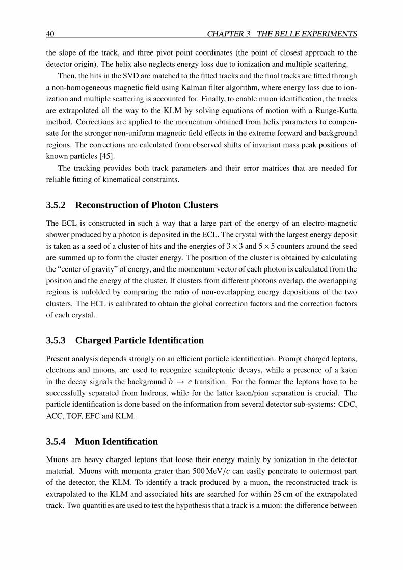
40 CHAPTER 3. THE BELLE EXPERIMENTS
the slope of the track, and three pivot point coordinates (the point of closest approach to thedetector origin). The helix also neglects energy loss due to ionization and multiple scattering.
Then, the hits in the SVD are matched to the fitted tracks and the final tracks are fitted througha non-homogeneous magnetic field using Kalman filter algorithm, where energy loss due to ion-ization and multiple scattering is accounted for. Finally, to enable muon identification, the tracksare extrapolated all the way to the KLM by solving equations of motion with a Runge-Kuttamethod. Corrections are applied to the momentum obtained from helix parameters to compen-sate for the stronger non-uniform magnetic field effects in the extreme forward and backgroundregions. The corrections are calculated from observed shifts of invariant mass peak positions ofknown particles [45].
The tracking provides both track parameters and their error matrices that are needed forreliable fitting of kinematical constraints.
3.5.2 Reconstruction of Photon Clusters
The ECL is constructed in such a way that a large part of the energy of an electro-magneticshower produced by a photon is deposited in the ECL. The crystal with the largest energy depositis taken as a seed of a cluster of hits and the energies of 3 × 3 and 5 × 5 counters around the seedare summed up to form the cluster energy. The position of the cluster is obtained by calculatingthe “center of gravity” of energy, and the momentum vector of each photon is calculated from theposition and the energy of the cluster. If clusters from different photons overlap, the overlappingregions is unfolded by comparing the ratio of non-overlapping energy depositions of the twoclusters. The ECL is calibrated to obtain the global correction factors and the correction factorsof each crystal.
3.5.3 Charged Particle Identification
Present analysis depends strongly on an efficient particle identification. Prompt charged leptons,electrons and muons, are used to recognize semileptonic decays, while a presence of a kaonin the decay signals the background b → c transition. For the former the leptons have to besuccessfully separated from hadrons, while for the latter kaon/pion separation is crucial. Theparticle identification is done based on the information from several detector sub-systems: CDC,ACC, TOF, EFC and KLM.
3.5.4 Muon Identification
Muons are heavy charged leptons that loose their energy mainly by ionization in the detectormaterial. Muons with momenta grater than 500 MeV/c can easily penetrate to outermost partof the detector, the KLM. To identify a track produced by a muon, the reconstructed track isextrapolated to the KLM and associated hits are searched for within 25 cm of the extrapolatedtrack. Two quantities are used to test the hypothesis that a track is a muon: the difference between
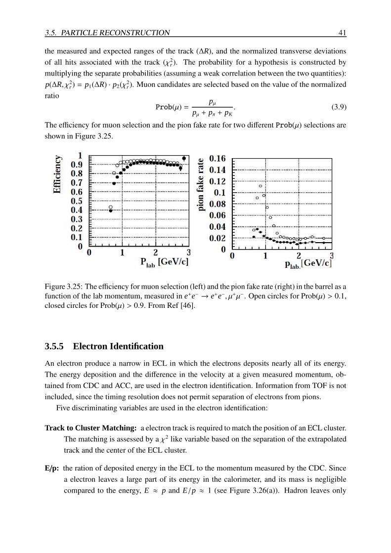
3.5. PARTICLE RECONSTRUCTION 41
the measured and expected ranges of the track (∆R), and the normalized transverse deviationsof all hits associated with the track (χ2
r ). The probability for a hypothesis is constructed bymultiplying the separate probabilities (assuming a weak correlation between the two quantities):p(∆R, χ2
r ) = p1(∆R) · p2(χ2r ). Muon candidates are selected based on the value of the normalized
ratioProb(µ) =
pµpµ + pπ + pK
. (3.9)
The efficiency for muon selection and the pion fake rate for two different Prob(µ) selections areshown in Figure 3.25.
Figure 3.25: The efficiency for muon selection (left) and the pion fake rate (right) in the barrel as afunction of the lab momentum, measured in e+e− → e+e−, µ+µ−. Open circles for Prob(µ) > 0.1,closed circles for Prob(µ) > 0.9. From Ref [46].
3.5.5 Electron Identification
An electron produce a narrow in ECL in which the electrons deposits nearly all of its energy.The energy deposition and the difference in the velocity at a given measured momentum, ob-tained from CDC and ACC, are used in the electron identification. Information from TOF is notincluded, since the timing resolution does not permit separation of electrons from pions.
Five discriminating variables are used in the electron identification:
Track to Cluster Matching: a electron track is required to match the position of an ECL cluster.The matching is assessed by a χ2 like variable based on the separation of the extrapolatedtrack and the center of the ECL cluster.
E/p: the ration of deposited energy in the ECL to the momentum measured by the CDC. Sincea electron leaves a large part of its energy in the calorimeter, and its mass is negligiblecompared to the energy, E ≈ p and E/p ≈ 1 (see Figure 3.26(a)). Hadron leaves only
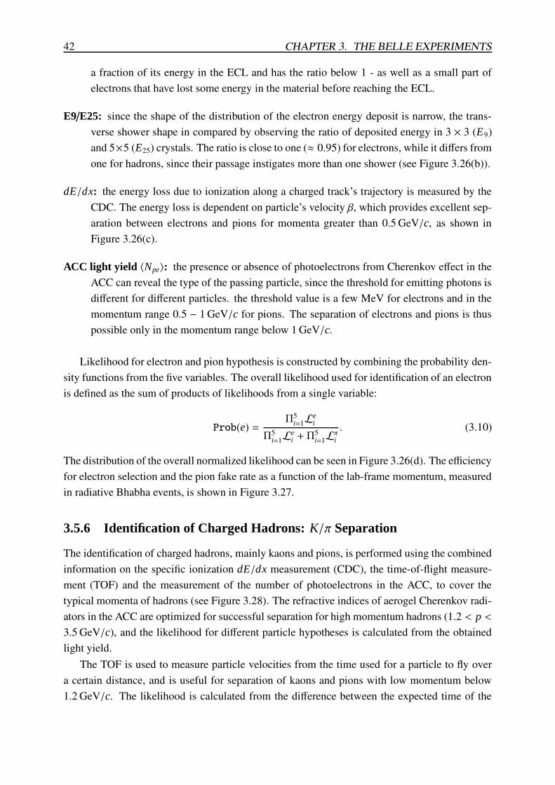
42 CHAPTER 3. THE BELLE EXPERIMENTS
a fraction of its energy in the ECL and has the ratio below 1 - as well as a small part ofelectrons that have lost some energy in the material before reaching the ECL.
E9/E25: since the shape of the distribution of the electron energy deposit is narrow, the trans-verse shower shape in compared by observing the ratio of deposited energy in 3 × 3 (E9)and 5×5 (E25) crystals. The ratio is close to one (≈ 0.95) for electrons, while it differs fromone for hadrons, since their passage instigates more than one shower (see Figure 3.26(b)).
dE/dx: the energy loss due to ionization along a charged track’s trajectory is measured by theCDC. The energy loss is dependent on particle’s velocity β, which provides excellent sep-aration between electrons and pions for momenta greater than 0.5 GeV/c, as shown inFigure 3.26(c).
ACC light yield 〈Npe〉: the presence or absence of photoelectrons from Cherenkov effect in theACC can reveal the type of the passing particle, since the threshold for emitting photons isdifferent for different particles. the threshold value is a few MeV for electrons and in themomentum range 0.5 − 1 GeV/c for pions. The separation of electrons and pions is thuspossible only in the momentum range below 1 GeV/c.
Likelihood for electron and pion hypothesis is constructed by combining the probability den-sity functions from the five variables. The overall likelihood used for identification of an electronis defined as the sum of products of likelihoods from a single variable:
Prob(e) =Π5
i=1Lei
Π5i=1Le
i + Π5i=1Lπi
. (3.10)
The distribution of the overall normalized likelihood can be seen in Figure 3.26(d). The efficiencyfor electron selection and the pion fake rate as a function of the lab-frame momentum, measuredin radiative Bhabha events, is shown in Figure 3.27.
3.5.6 Identification of Charged Hadrons: K/π Separation
The identification of charged hadrons, mainly kaons and pions, is performed using the combinedinformation on the specific ionization dE/dx measurement (CDC), the time-of-flight measure-ment (TOF) and the measurement of the number of photoelectrons in the ACC, to cover thetypical momenta of hadrons (see Figure 3.28). The refractive indices of aerogel Cherenkov radi-ators in the ACC are optimized for successful separation for high momentum hadrons (1.2 < p <
3.5 GeV/c), and the likelihood for different particle hypotheses is calculated from the obtainedlight yield.
The TOF is used to measure particle velocities from the time used for a particle to fly overa certain distance, and is useful for separation of kaons and pions with low momentum below1.2 GeV/c. The likelihood is calculated from the difference between the expected time of the
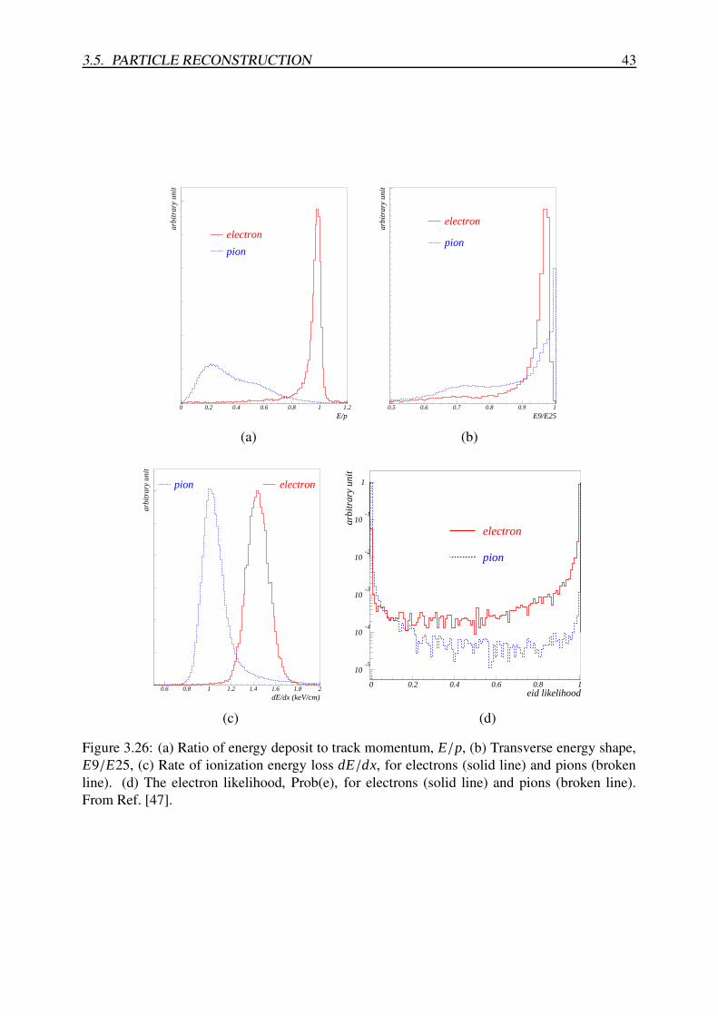
3.5. PARTICLE RECONSTRUCTION 43
0
0.02
0.04
0.06
0.08
0.1
0.12
0 0.2 0.4 0.6 0.8 1 1.2
electron
pion
E/p
arbi
trar
y un
it
0
0.025
0.05
0.075
0.1
0.125
0.15
0.175
0.2
0.5 0.6 0.7 0.8 0.9 1
electron
pion
E9/E25
arbi
trar
y un
it
(a) (b)
0
0.01
0.02
0.03
0.04
0.05
0.06
0.6 0.8 1 1.2 1.4 1.6 1.8 2
electronpion
dE/dx (keV/cm)
arbi
trar
y un
it
10-5
10-4
10-3
10-2
10-1
1
0 0.2 0.4 0.6 0.8 1
pion
electron
eid likelihood
arbi
trar
y un
it
(c) (d)
Figure 3.26: (a) Ratio of energy deposit to track momentum, E/p, (b) Transverse energy shape,E9/E25, (c) Rate of ionization energy loss dE/dx, for electrons (solid line) and pions (brokenline). (d) The electron likelihood, Prob(e), for electrons (solid line) and pions (broken line).From Ref. [47].
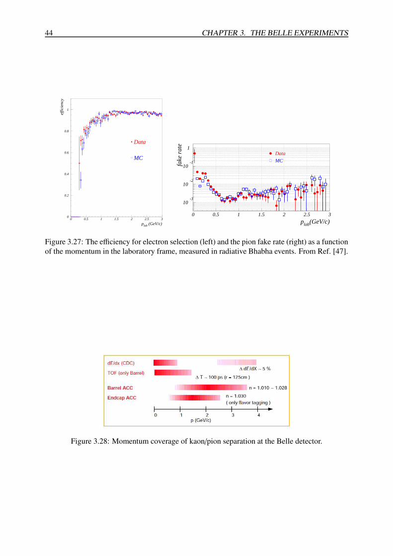
44 CHAPTER 3. THE BELLE EXPERIMENTS
0
0.2
0.4
0.6
0.8
1
0 0.5 1 1.5 2 2.5 3
Data
MC
plab (GeV/c)
effi
cien
cy
10-3
10-2
10-1
1
0 0.5 1 1.5 2 2.5 3
Data
MC
plab(GeV/c)
fake
rat
e
Figure 3.27: The efficiency for electron selection (left) and the pion fake rate (right) as a functionof the momentum in the laboratory frame, measured in radiative Bhabha events. From Ref. [47].
Figure 3.28: Momentum coverage of kaon/pion separation at the Belle detector.
3.5. PARTICLE RECONSTRUCTION 45
flight for a hypothesis and the measured time:
LTOF =e−
12χ
2TOF
√2πσTOF
, χ2TOF =
[
tmeas − thyp
σTOF
]2
. (3.11)
Similarly, the likelihood obtained from the measurement of ionization loss is obtained as:
LdE/dx =e−
12χ
2dE/dx
√2πσdE/dx
, χ2dE/dx =
[ (dE/dx)meas − (dE/dx)hyp
σdE/dx
]2
. (3.12)
The total likelihood of a hypothesis is obtained as the product of three kinds of the likelihood:
L = LACC(hyp) × LTOF(hyp) × LdE/dx(hyp). (3.13)
The separation of charged hadrons is achieved by calculating the probability .Prob(signal/background) of the signal particle hypothesis, when separating it from the
background particle. The probability is calculated from the likelihoods of signal and backgroundhypotheses:
Prob(signal/background) =L(signal)
L(signal) +L(background) . (3.14)
The signal and background particles can be any of the following: e, p,K, π. The kaon selectionefficiency and the pion fake rate for Prob(K/π) > 0.6 is shown in Figure 3.13.

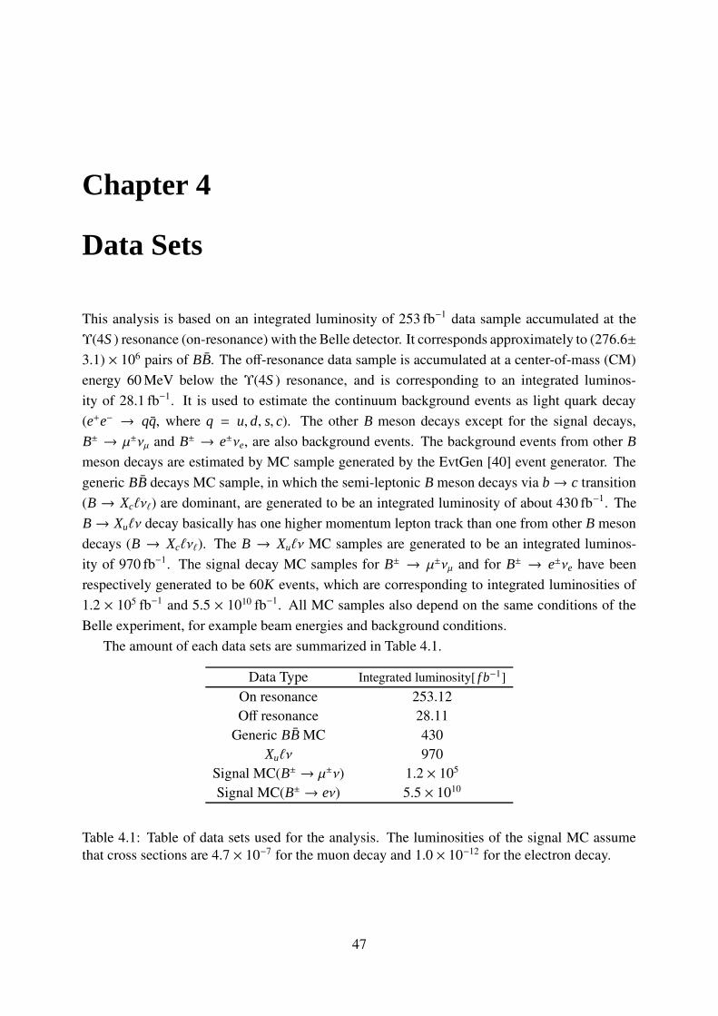
Chapter 4
Data Sets
This analysis is based on an integrated luminosity of 253 fb−1 data sample accumulated at theΥ(4S ) resonance (on-resonance) with the Belle detector. It corresponds approximately to (276.6±3.1) × 106 pairs of BB. The off-resonance data sample is accumulated at a center-of-mass (CM)energy 60 MeV below the Υ(4S ) resonance, and is corresponding to an integrated luminos-ity of 28.1 fb−1. It is used to estimate the continuum background events as light quark decay(e+e− → qq, where q = u, d, s, c). The other B meson decays except for the signal decays,B± → µ±νµ and B± → e±νe, are also background events. The background events from other B
meson decays are estimated by MC sample generated by the EvtGen [40] event generator. Thegeneric BB decays MC sample, in which the semi-leptonic B meson decays via b→ c transition(B → Xc`ν`) are dominant, are generated to be an integrated luminosity of about 430 fb−1. TheB → Xu`ν decay basically has one higher momentum lepton track than one from other B mesondecays (B → Xc`ν`). The B → Xu`ν MC samples are generated to be an integrated luminos-ity of 970 fb−1. The signal decay MC samples for B± → µ±νµ and for B± → e±νe have beenrespectively generated to be 60K events, which are corresponding to integrated luminosities of1.2 × 105 fb−1 and 5.5 × 10¹⁰ fb−1. All MC samples also depend on the same conditions of theBelle experiment, for example beam energies and background conditions.
The amount of each data sets are summarized in Table 4.1.
Data Type Integrated luminosity[ f b−1]On resonance 253.12Off resonance 28.11
Generic BB MC 430Xu`ν 970
Signal MC(B± → µ±ν) 1.2 × 10⁵
Signal MC(B± → eν) 5.5 × 10¹⁰
Table 4.1: Table of data sets used for the analysis. The luminosities of the signal MC assumethat cross sections are 4.7 × 10⁻⁷ for the muon decay and 1.0 × 10⁻¹² for the electron decay.
47

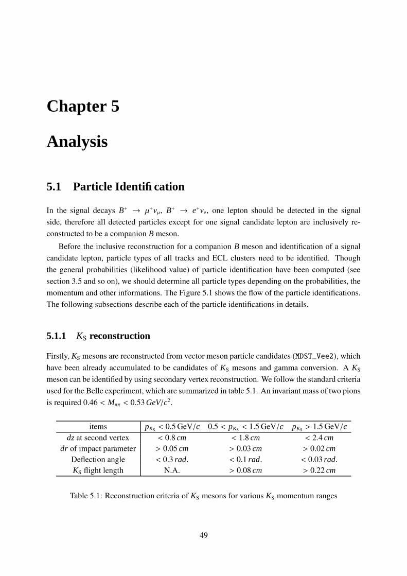
Chapter 5
Analysis
5.1 Particle Identification
In the signal decays B+ → µ+νµ, B+ → e+νe, one lepton should be detected in the signalside, therefore all detected particles except for one signal candidate lepton are inclusively re-constructed to be a companion B meson.
Before the inclusive reconstruction for a companion B meson and identification of a signalcandidate lepton, particle types of all tracks and ECL clusters need to be identified. Thoughthe general probabilities (likelihood value) of particle identification have been computed (seesection 3.5 and so on), we should determine all particle types depending on the probabilities, themomentum and other informations. The Figure 5.1 shows the flow of the particle identifications.The following subsections describe each of the particle identifications in details.
5.1.1 KS reconstruction
Firstly, KS mesons are reconstructed from vector meson particle candidates (MDST_Vee2), whichhave been already accumulated to be candidates of KS mesons and gamma conversion. A KS
meson can be identified by using secondary vertex reconstruction. We follow the standard criteriaused for the Belle experiment, which are summarized in table 5.1. An invariant mass of two pionsis required 0.46 < Mππ < 0.53 GeV/c2.
items pKS < 0.5 GeV/c 0.5 < pKS < 1.5 GeV/c pKS > 1.5 GeV/cdz at second vertex < 0.8 cm < 1.8 cm < 2.4 cm
dr of impact parameter > 0.05 cm > 0.03 cm > 0.02 cmDeflection angle < 0.3 rad. < 0.1 rad. < 0.03 rad.KS flight length N.A. > 0.08 cm > 0.22 cm
Table 5.1: Reconstruction criteria of KS mesons for various KS momentum ranges
49
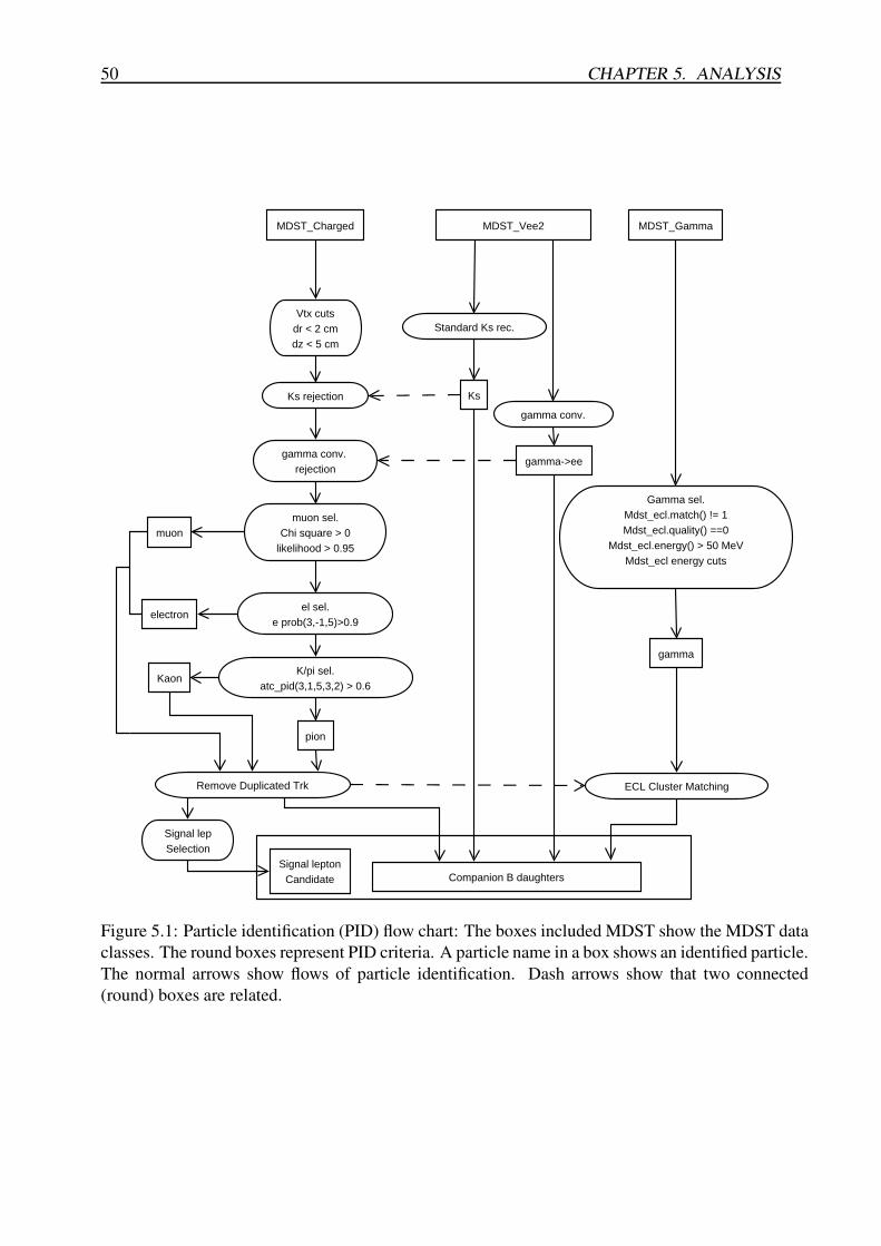
50 CHAPTER 5. ANALYSIS
MDST_Charged MDST_Vee2 MDST_Gamma
Vtx cutsdr < 2 cmdz < 5 cm
Ks rejection
gamma conv. rejection
muon sel.Chi square > 0
likelihood > 0.95
el sel.e prob(3,-1,5)>0.9
K/pi sel.atc_pid(3,1,5,3,2) > 0.6
muon
electron
Kaon
pion
Standard Ks rec.
gamma conv.
Companion B daughtersSignal lepton
Candidate
Gamma sel.Mdst_ecl.match() != 1Mdst_ecl.quality() ==0
Mdst_ecl.energy() > 50 MeVMdst_ecl energy cuts
Remove Duplicated Trk ECL Cluster Matching
Ks
gamma->ee
Signal lepSelection
gamma
Figure 5.1: Particle identification (PID) flow chart: The boxes included MDST show the MDST dataclasses. The round boxes represent PID criteria. A particle name in a box shows an identified particle.The normal arrows show flows of particle identification. Dash arrows show that two connected(round) boxes are related.

5.1. PARTICLE IDENTIFICATION 51
5.1.2 Reconstruction of γ Conversion
Some of γs passing through the Belle detector are converted into electron-positron pairs throughthe electromagnetic interaction. The events are called γ(photon) conversion. They are recon-structed from MDST_Vee2 An invariant mass of an electron-positron pair are required Mee <
0.1 GeV/c2.
5.1.3 Identification of Charged Particle
All charged tracks are accumulated in the MDST_Charged data. Charged tracks are classifiedfour kinds of particles, which are muon, electron, kaon and pion. If a charged track has beenreconstructed to be a KS meson or γ conversion, it is explicitly vetoed. We require tight iden-tification criteria for leptons in order to reject punch-through pions and kaons polluting leptonpurity in higher momentum region. The following criteria are required for charged tracks.
• length of radial direction cut : dr < 2.0 cm
• length of beam axis cut : dz < 5.0 cm
• Particles reconstructed to be KS and photon conversion are vetoed.
• Remove duplicated tracks (See next section)
The following criteria are required for the determination of particle type.
• µ : muon probability > 0.95 (see section 3.5.5)
• e : electron probability > 0.9 (see section 3.5.4)
• K : kaon probability > 0.6 (see section 3.5.6)
• π : otherwise failing the criteria for µ, e and K
Duplicated tracks
For the identified charged particles, we check whether they are the fake track or not. When thetransverse momentum(pT ) of the track is as low as it curls back inside of the CDC, and the trackfinder sometimes makes duplicated tracks (see Figure 5.2). The duplicated tracks may have thesame or opposite charge of the original track. A duplicated pair with the same charge have thealmost same transverse momentum and the opening angle (φ2tracks) between the original track andthe same charge duplicated track should be small. A duplicated pair with opposite charge havealmost same momentum but the opening angle is close to 180◦. We use information based on theimpact parameters. A pair of duplicated tracks are defined as follows:
• same charge : ∆pT < 0.1 GeV/c and cos φ2tracks < 0.9
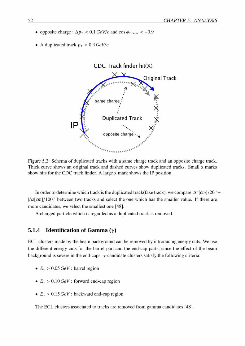
52 CHAPTER 5. ANALYSIS
• opposite charge : ∆pT < 0.1 GeV/c and cos φ2tracks < −0.9
• A duplicated track pT < 0.3 GeV/c
Figure 5.2: Schema of duplicated tracks with a same charge track and an opposite charge track.Thick curve shows an original track and dashed curves show duplicated tracks. Small x marksshow hits for the CDC track finder. A large x mark shows the IP position.
In order to determine which track is the duplicated track(fake track), we compare |∆r[cm]/20|2+|∆z[cm]/100|2 between two tracks and select the one which has the smaller value. If there aremore candidates, we select the smallest one [48].
A charged particle which is regarded as a duplicated track is removed.
5.1.4 Identification of Gamma (γ)
ECL clusters made by the beam background can be removed by introducing energy cuts. We usethe different energy cuts for the barrel part and the end-cap parts, since the effect of the beambackground is severe in the end-caps. γ-candidate clusters satisfy the following criteria:
• Eγ > 0.05 GeV : barrel region
• Eγ > 0.10 GeV : forward end-cap region
• Eγ > 0.15 GeV : backward end-cap region
The ECL clusters associated to tracks are removed from gamma candidates [48].
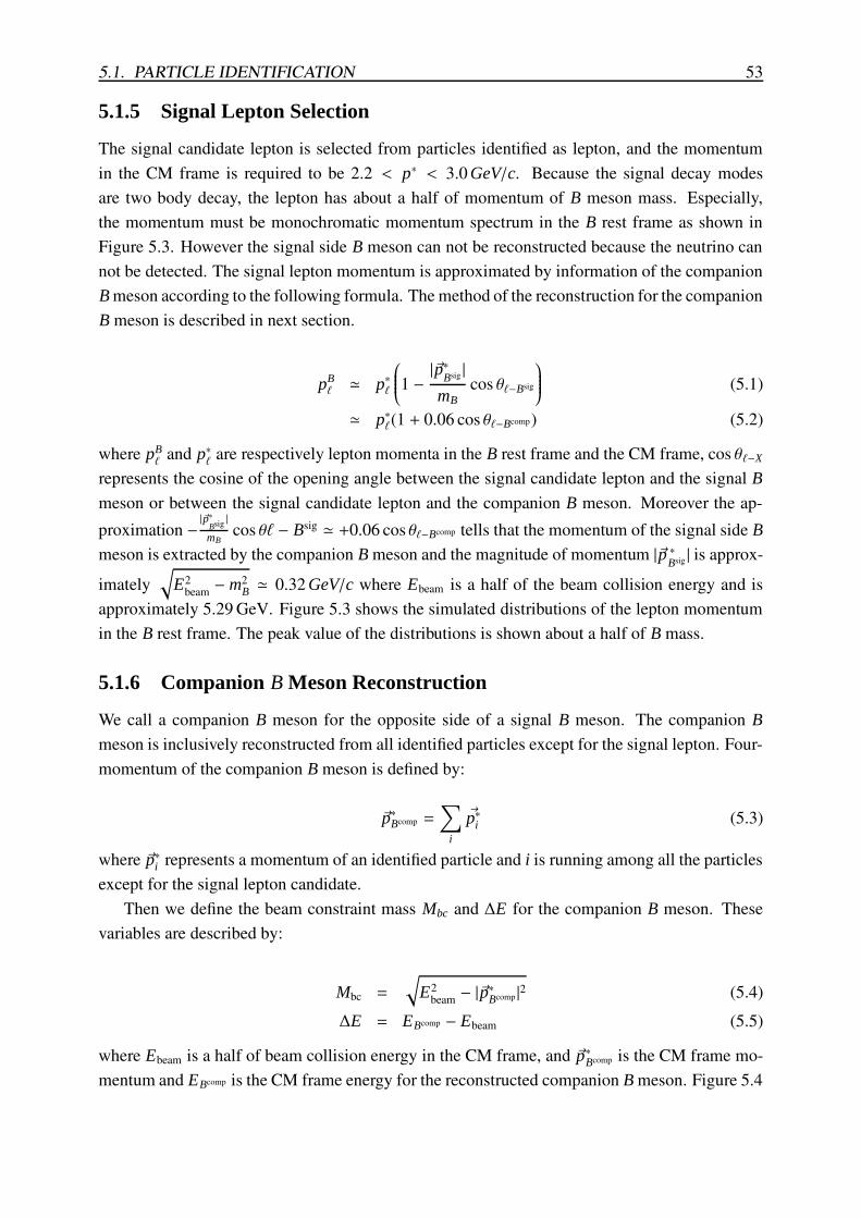
5.1. PARTICLE IDENTIFICATION 53
5.1.5 Signal Lepton Selection
The signal candidate lepton is selected from particles identified as lepton, and the momentumin the CM frame is required to be 2.2 < p∗ < 3.0 GeV/c. Because the signal decay modesare two body decay, the lepton has about a half of momentum of B meson mass. Especially,the momentum must be monochromatic momentum spectrum in the B rest frame as shown inFigure 5.3. However the signal side B meson can not be reconstructed because the neutrino cannot be detected. The signal lepton momentum is approximated by information of the companionB meson according to the following formula. The method of the reconstruction for the companionB meson is described in next section.
pB` ' p∗`
1 −|~p∗
Bsig |mB
cos θ`−Bsig
(5.1)
' p∗`(1 + 0.06 cos θ`−Bcomp) (5.2)
where pB` and p∗` are respectively lepton momenta in the B rest frame and the CM frame, cos θ`−X
represents the cosine of the opening angle between the signal candidate lepton and the signal B
meson or between the signal candidate lepton and the companion B meson. Moreover the ap-proximation −
|~p∗Bsig |mB
cos θ` − Bsig ' +0.06 cos θ`−Bcomp tells that the momentum of the signal side B
meson is extracted by the companion B meson and the magnitude of momentum |~p ∗Bsig | is approx-
imately√
E2beam − m2
B ' 0.32 GeV/c where Ebeam is a half of the beam collision energy and isapproximately 5.29 GeV. Figure 5.3 shows the simulated distributions of the lepton momentumin the B rest frame. The peak value of the distributions is shown about a half of B mass.
5.1.6 Companion B Meson Reconstruction
We call a companion B meson for the opposite side of a signal B meson. The companion B
meson is inclusively reconstructed from all identified particles except for the signal lepton. Four-momentum of the companion B meson is defined by:
~p∗Bcomp =∑
i
~p∗i (5.3)
where ~p∗i represents a momentum of an identified particle and i is running among all the particlesexcept for the signal lepton candidate.
Then we define the beam constraint mass Mbc and ∆E for the companion B meson. Thesevariables are described by:
Mbc =
√
E2beam − |~p∗Bcomp |2 (5.4)
∆E = EBcomp − Ebeam (5.5)
where Ebeam is a half of beam collision energy in the CM frame, and ~p∗Bcomp is the CM frame mo-mentum and EBcomp is the CM frame energy for the reconstructed companion B meson. Figure 5.4
54 CHAPTER 5. ANALYSIS
[GeV/c]BlP
2.1 2.2 2.3 2.4 2.5 2.6 2.7 2.8 2.9 3 3.1
arb
ito
rary
muon
electron
Figure 5.3: pB` distribution for the signal MC samples, where pB
` represents the lepton momentum inthe B rest frame.
and Figure 5.5 show the Mbc and ∆E distributions for each decay mode after pre-selections (seenext section) have been applied, respectively. If collection of the companion B mesons are cor-rect, the Mbc distribution have a peak at 5.28 GeV/c2 like a signal MC distribution.
5.2 Event Selection
In this section, we explain the event selection and its optimization. Firstly, the pre-selectionwhich have been already applied to all data samples at the event selection stage is described. Thedefinitions of the signal region, the fit region and the sideband region are also described. Afterthe above explanation have done, the event selection is described. The selection is classifiedinto three sections by the features of the selection. The event selection is constraints on thesignal candidate lepton, continuum suppression and neutrino reconstruction. They are explainedaccording to this order. Finally all selection criteria are determined by the results of the selectionoptimization.
5.2.1 Pre-selection
Most of the events collected by the Belle detector are obviously irrelevant events for this analysisand are removed in advance of the event selection. The number of tracks identified lepton islimited to one, the momentum of the signal candidate lepton in the CM frame is also limited andMbc is required as follows:
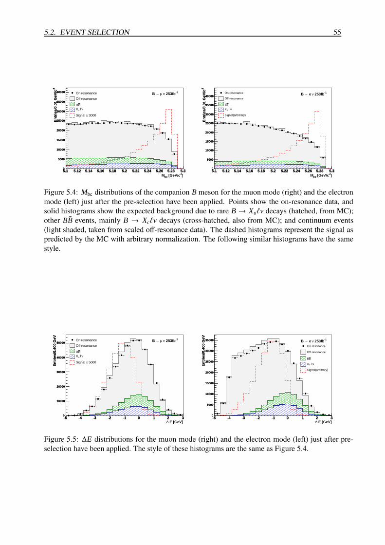
5.2. EVENT SELECTION 55
5.1 5.12 5.14 5.16 5.18 5.2 5.22 5.24 5.26 5.28 5.3
2E
ntr
ies/
0.01
GeV
/c
0
5000
10000
15000
20000
25000
30000
35000
40000
]2 [GeV/cbcM5.1 5.12 5.14 5.16 5.18 5.2 5.22 5.24 5.26 5.28 5.3
2E
ntr
ies/
0.01
GeV
/c
0
5000
10000
15000
20000
25000
30000
35000
40000 On resonance
Off resonance
BBν l uX
Signal x 3000
-1 253fbν µ →B
5.1 5.12 5.14 5.16 5.18 5.2 5.22 5.24 5.26 5.28 5.3
2E
ntr
ies/
0.01
GeV
/c
0
5000
10000
15000
20000
25000
30000
35000
40000
]2 [GeV/cbcM5.1 5.12 5.14 5.16 5.18 5.2 5.22 5.24 5.26 5.28 5.3
2E
ntr
ies/
0.01
GeV
/c
0
5000
10000
15000
20000
25000
30000
35000
40000On resonance
Off resonance
BB
ν l uX
Signal(arbitrary)
-1 253fbν e →B
Figure 5.4: Mbc distributions of the companion B meson for the muon mode (right) and the electronmode (left) just after the pre-selection have been applied. Points show the on-resonance data, andsolid histograms show the expected background due to rare B → Xu`ν decays (hatched, from MC);other BB events, mainly B → Xc`ν decays (cross-hatched, also from MC); and continuum events(light shaded, taken from scaled off-resonance data). The dashed histograms represent the signal aspredicted by the MC with arbitrary normalization. The following similar histograms have the samestyle.
-5 -4 -3 -2 -1 0 1 2 3
En
trie
s/0.
400
GeV
0
10000
20000
30000
40000
50000
E [GeV]∆-5 -4 -3 -2 -1 0 1 2 3
En
trie
s/0.
400
GeV
0
10000
20000
30000
40000
50000On resonance
Off resonance
BBν l uX
Signal x 5000
-1 253fbν µ →B
-5 -4 -3 -2 -1 0 1 2 3
En
trie
s/0.
400
GeV
0
5000
10000
15000
20000
25000
30000
35000
E [GeV]∆-5 -4 -3 -2 -1 0 1 2 3
En
trie
s/0.
400
GeV
0
5000
10000
15000
20000
25000
30000
35000
On resonance
Off resonance
BB
ν l uX
Signal(arbitrary)
-1 253fbν e →B
Figure 5.5: ∆E distributions for the muon mode (right) and the electron mode (left) just after pre-selection have been applied. The style of these histograms are the same as Figure 5.4.
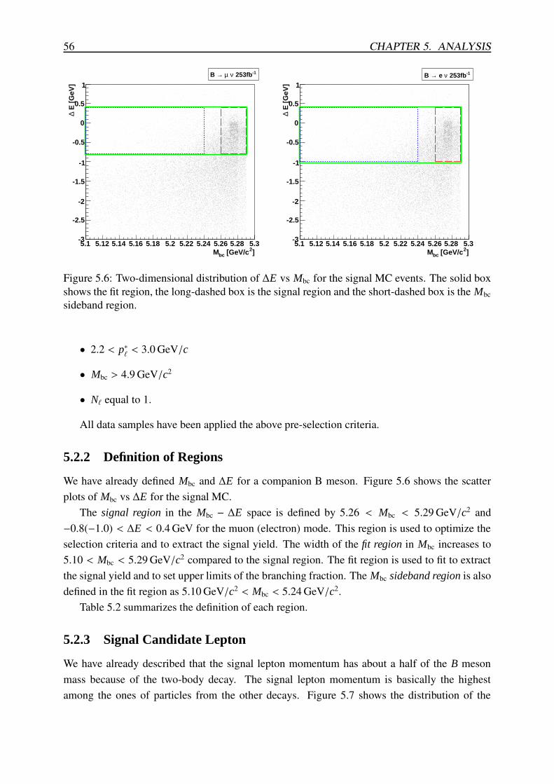
56 CHAPTER 5. ANALYSIS
]2 [GeV/cbcM5.1 5.12 5.14 5.16 5.18 5.2 5.22 5.24 5.26 5.28 5.3
E [
GeV
]∆
-3
-2.5
-2
-1.5
-1
-0.5
0
0.5
1
-1 253fbν µ →B
]2 [GeV/cbcM5.1 5.12 5.14 5.16 5.18 5.2 5.22 5.24 5.26 5.28 5.3
E [
GeV
]∆
-3
-2.5
-2
-1.5
-1
-0.5
0
0.5
1
-1 253fbν e →B
Figure 5.6: Two-dimensional distribution of ∆E vs Mbc for the signal MC events. The solid boxshows the fit region, the long-dashed box is the signal region and the short-dashed box is the Mbcsideband region.
• 2.2 < p∗` < 3.0 GeV/c
• Mbc > 4.9 GeV/c2
• N` equal to 1.
All data samples have been applied the above pre-selection criteria.
5.2.2 Definition of Regions
We have already defined Mbc and ∆E for a companion B meson. Figure 5.6 shows the scatterplots of Mbc vs ∆E for the signal MC.
The signal region in the Mbc − ∆E space is defined by 5.26 < Mbc < 5.29 GeV/c2 and−0.8(−1.0) < ∆E < 0.4 GeV for the muon (electron) mode. This region is used to optimize theselection criteria and to extract the signal yield. The width of the fit region in Mbc increases to5.10 < Mbc < 5.29 GeV/c2 compared to the signal region. The fit region is used to fit to extractthe signal yield and to set upper limits of the branching fraction. The Mbc sideband region is alsodefined in the fit region as 5.10 GeV/c2 < Mbc < 5.24 GeV/c2.
Table 5.2 summarizes the definition of each region.
5.2.3 Signal Candidate Lepton
We have already described that the signal lepton momentum has about a half of the B mesonmass because of the two-body decay. The signal lepton momentum is basically the highestamong the ones of particles from the other decays. Figure 5.7 shows the distribution of the
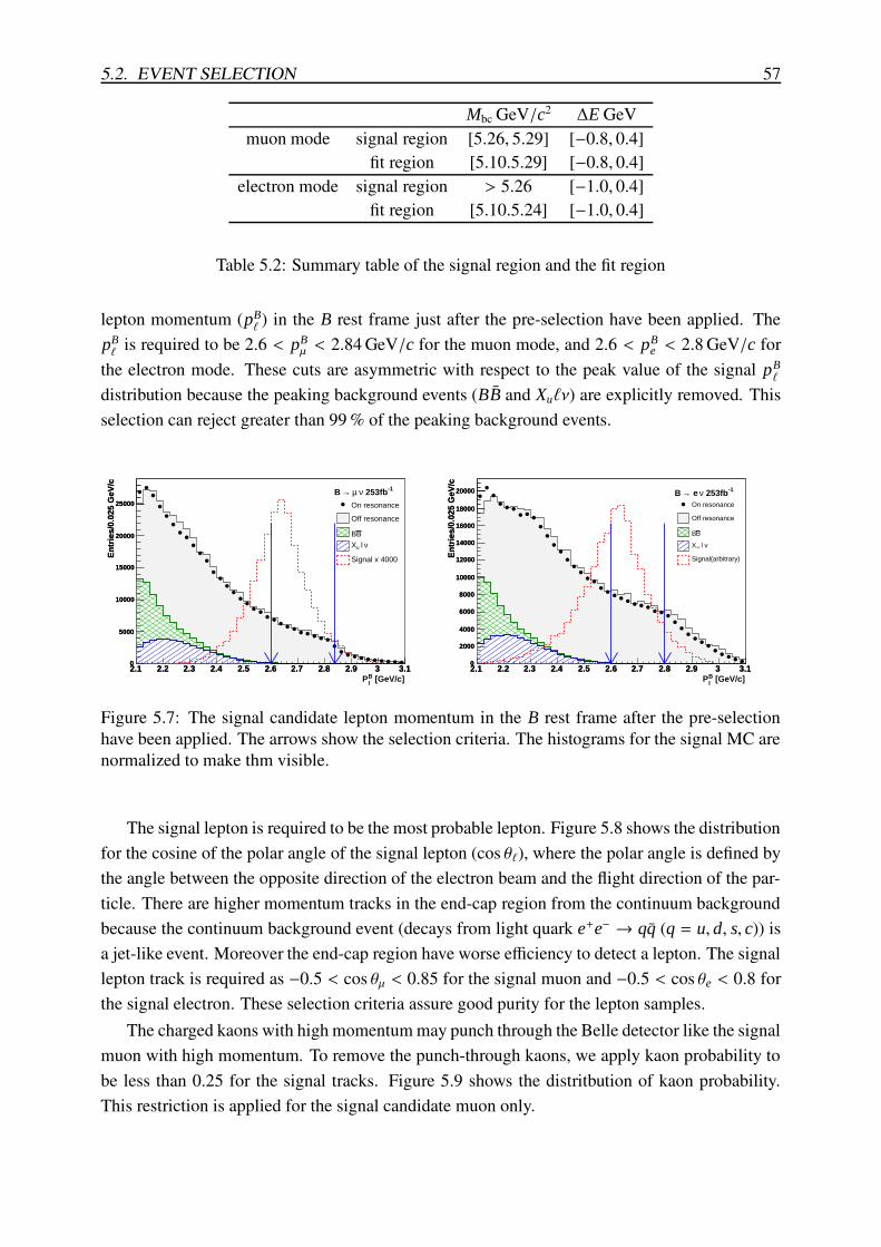
5.2. EVENT SELECTION 57
Mbc GeV/c2 ∆E GeVmuon mode signal region [5.26, 5.29] [−0.8, 0.4]
fit region [5.10.5.29] [−0.8, 0.4]electron mode signal region > 5.26 [−1.0, 0.4]
fit region [5.10.5.24] [−1.0, 0.4]
Table 5.2: Summary table of the signal region and the fit region
lepton momentum (pB` ) in the B rest frame just after the pre-selection have been applied. The
pB` is required to be 2.6 < pB
µ < 2.84 GeV/c for the muon mode, and 2.6 < pBe < 2.8 GeV/c for
the electron mode. These cuts are asymmetric with respect to the peak value of the signal pB`
distribution because the peaking background events (BB and Xu`ν) are explicitly removed. Thisselection can reject greater than 99 % of the peaking background events.
2.1 2.2 2.3 2.4 2.5 2.6 2.7 2.8 2.9 3 3.1
En
trie
s/0.
025
GeV
/c
0
5000
10000
15000
20000
25000
[GeV/c]BlP
2.1 2.2 2.3 2.4 2.5 2.6 2.7 2.8 2.9 3 3.1
En
trie
s/0.
025
GeV
/c
0
5000
10000
15000
20000
25000 On resonance
Off resonance
BB
ν l uX
Signal x 4000
-1 253fbν µ →B
2.1 2.2 2.3 2.4 2.5 2.6 2.7 2.8 2.9 3 3.1
En
trie
s/0.
025
GeV
/c
0
2000
4000
6000
8000
10000
12000
14000
16000
18000
20000
[GeV/c]BlP
2.1 2.2 2.3 2.4 2.5 2.6 2.7 2.8 2.9 3 3.1
En
trie
s/0.
025
GeV
/c
0
2000
4000
6000
8000
10000
12000
14000
16000
18000
20000
On resonance
Off resonance
BB
ν l uX
Signal(arbitrary)
-1 253fbν e →B
Figure 5.7: The signal candidate lepton momentum in the B rest frame after the pre-selectionhave been applied. The arrows show the selection criteria. The histograms for the signal MC arenormalized to make thm visible.
The signal lepton is required to be the most probable lepton. Figure 5.8 shows the distributionfor the cosine of the polar angle of the signal lepton (cos θ`), where the polar angle is defined bythe angle between the opposite direction of the electron beam and the flight direction of the par-ticle. There are higher momentum tracks in the end-cap region from the continuum backgroundbecause the continuum background event (decays from light quark e+e− → qq (q = u, d, s, c)) isa jet-like event. Moreover the end-cap region have worse efficiency to detect a lepton. The signallepton track is required as −0.5 < cos θµ < 0.85 for the signal muon and −0.5 < cos θe < 0.8 forthe signal electron. These selection criteria assure good purity for the lepton samples.
The charged kaons with high momentum may punch through the Belle detector like the signalmuon with high momentum. To remove the punch-through kaons, we apply kaon probability tobe less than 0.25 for the signal tracks. Figure 5.9 shows the distritbution of kaon probability.This restriction is applied for the signal candidate muon only.
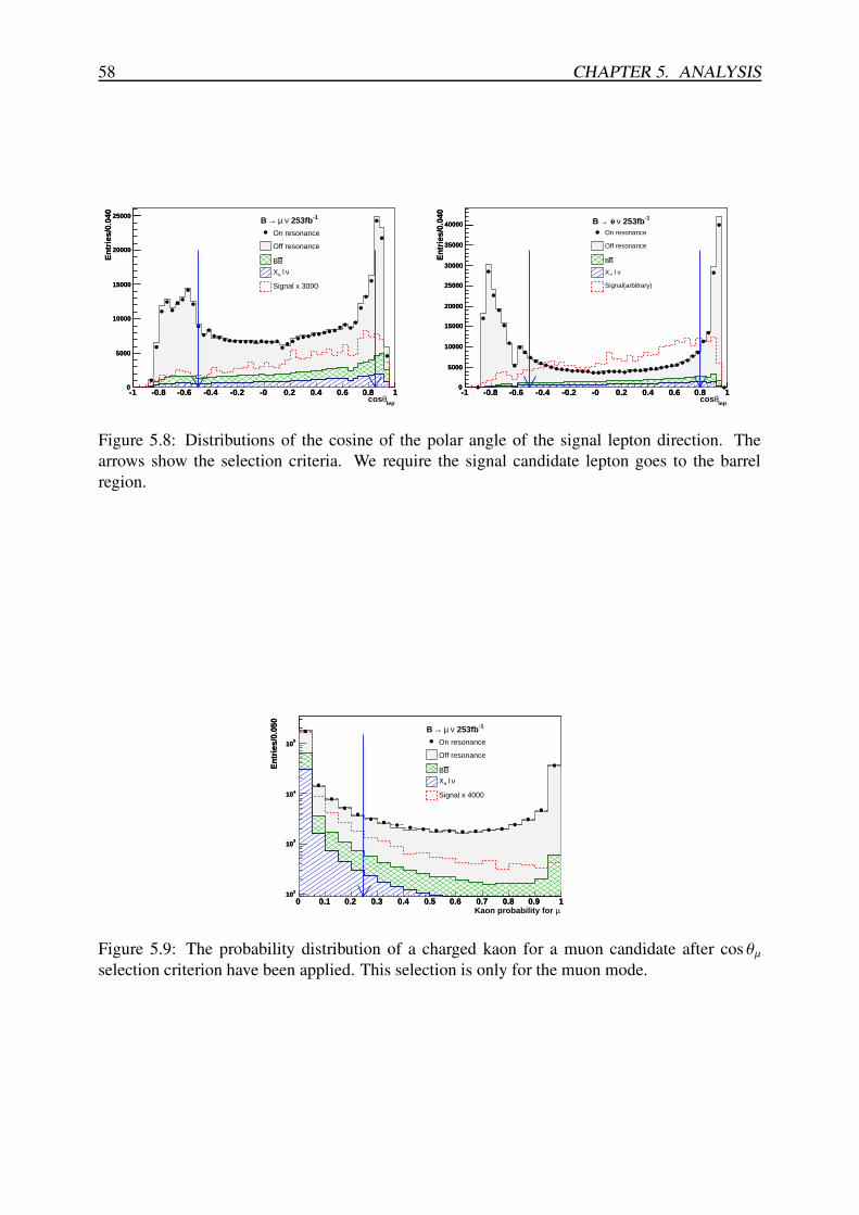
58 CHAPTER 5. ANALYSIS
-1 -0.8 -0.6 -0.4 -0.2 -0 0.2 0.4 0.6 0.8 1
En
trie
s/0.
040
0
5000
10000
15000
20000
25000
lepθcos-1 -0.8 -0.6 -0.4 -0.2 -0 0.2 0.4 0.6 0.8 1
En
trie
s/0.
040
0
5000
10000
15000
20000
25000
On resonance
Off resonance
BB
ν l uX
Signal x 3000
-1 253fbν µ →B
-1 -0.8 -0.6 -0.4 -0.2 -0 0.2 0.4 0.6 0.8 1
En
trie
s/0.
040
0
5000
10000
15000
20000
25000
30000
35000
40000
lepθcos-1 -0.8 -0.6 -0.4 -0.2 -0 0.2 0.4 0.6 0.8 1
En
trie
s/0.
040
0
5000
10000
15000
20000
25000
30000
35000
40000On resonance
Off resonance
BB
ν l uX
Signal(arbitrary)
-1 253fbν e →B
Figure 5.8: Distributions of the cosine of the polar angle of the signal lepton direction. Thearrows show the selection criteria. We require the signal candidate lepton goes to the barrelregion.
0 0.1 0.2 0.3 0.4 0.5 0.6 0.7 0.8 0.9 1
En
trie
s/0.
050
210
310
410
510
µKaon probability for 0 0.1 0.2 0.3 0.4 0.5 0.6 0.7 0.8 0.9 1
En
trie
s/0.
050
210
310
410
510 On resonance
Off resonance
BB
ν l uX
Signal x 4000
-1 253fbν µ →B
Figure 5.9: The probability distribution of a charged kaon for a muon candidate after cos θµselection criterion have been applied. This selection is only for the muon mode.
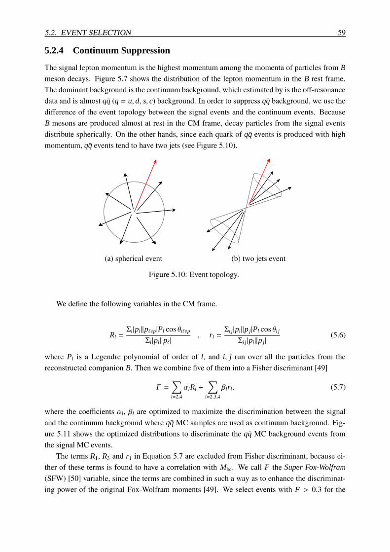
5.2. EVENT SELECTION 59
5.2.4 Continuum Suppression
The signal lepton momentum is the highest momentum among the momenta of particles from B
meson decays. Figure 5.7 shows the distribution of the lepton momentum in the B rest frame.The dominant background is the continuum background, which estimated by is the off-resonancedata and is almost qq (q = u, d, s, c) background. In order to suppress qq background, we use thedifference of the event topology between the signal events and the continuum events. BecauseB mesons are produced almost at rest in the CM frame, decay particles from the signal eventsdistribute spherically. On the other hands, since each quark of qq events is produced with highmomentum, qq events tend to have two jets (see Figure 5.10).
(a) spherical event (b) two jets event
Figure 5.10: Event topology.
We define the following variables in the CM frame.
Rl =Σi|pi||p`ep|Pl cos θi`ep
Σi|pi||p`|, rl =
Σi j|pi||p j|Pl cos θi j
Σi j|pi||p j|(5.6)
where Pl is a Legendre polynomial of order of l, and i, j run over all the particles from thereconstructed companion B. Then we combine five of them into a Fisher discriminant [49]
F =∑
l=2,4αlRl +
∑
l=2,3,4βlrl, (5.7)
where the coefficients αl, βl are optimized to maximize the discrimination between the signaland the continuum background where qq MC samples are used as continuum background. Fig-ure 5.11 shows the optimized distributions to discriminate the qq MC background events fromthe signal MC events.
The terms R1, R3 and r1 in Equation 5.7 are excluded from Fisher discriminant, because ei-ther of these terms is found to have a correlation with Mbc. We call F the Super Fox-Wolfram
(SFW) [50] variable, since the terms are combined in such a way as to enhance the discriminat-ing power of the original Fox-Wolfram moments [49]. We select events with F > 0.3 for the
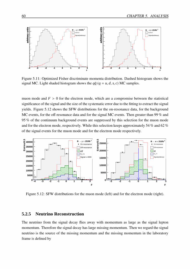
60 CHAPTER 5. ANALYSIS
-4 -3 -2 -1 0 1 2 3
arb
itra
ry u
nit
s
F-4 -3 -2 -1 0 1 2 3
arb
itra
ry u
nit
s
u,d,s,c
Signal(arbitrary)
-1 253fbν µ →B
-4 -3 -2 -1 0 1 2 3
arb
itra
ry u
nit
s
F-4 -3 -2 -1 0 1 2 3
arb
itra
ry u
nit
s
u,d,s,c
Signal(arbitrary)
-1 253fbν e →B
Figure 5.11: Optimized Fisher discriminate momenta distribution. Dashed histogram shows thesignal MC. Light shaded histogram shows the qq (q = u, d, s, c) MC samples.
muon mode and F > 0 for the electron mode, which are a compromise between the statisticalsignificance of the signal and the size of the systematic error due to the fitting to extract the signalyields. Figure 5.12 shows the SFW distributions for the on-resonance data, for the backgroundMC events, for the off-resonance data and for the signal MC events. Then greater than 99 % and95 % of the continuum background events are suppressed by this selection for the muon modeand for the electron mode, respectively. While this selection keeps approximately 54 % and 62 %of the signal events for the muon mode and for the electron mode respectively.
F
-4 -3 -2 -1 0 1 2 3
En
trie
s/0.
5
0
5000
10000
15000
20000
25000
30000
35000
40000On resonance
Off resonance
BBν l uX
Signal x 4000
-1 253fbν µ →B
F
-3 -2 -1 0 1 2 3
En
trie
s/0.
5
0
5000
10000
15000
20000
25000 On resonance
Off resonance
BB
ν l uX
Signal(arbitrary)
-1 253fbν e →B
Figure 5.12: SFW distributions for the muon mode (left) and for the electron mode (right).
5.2.5 Neutrino Reconstruction
The neutrino from the signal decay flies away with momentum as large as the signal leptonmomentum. Therefore the signal decay has large missing momentum. Then we regard the signalneutrino is the source of the missing momentum and the missing momentum in the laboratoryframe is defined by
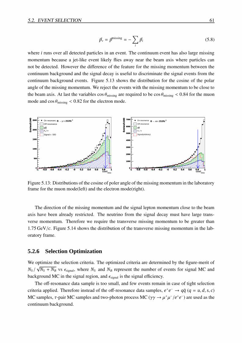
5.2. EVENT SELECTION 61
~pν = ~pmissing = −
∑
i
~pi (5.8)
where i runs over all detected particles in an event. The continuum event has also large missingmomentum because a jet-like event likely flies away near the beam axis where particles cannot be detected. However the difference of the feature for the missing momentum between thecontinuum background and the signal decay is useful to discriminate the signal events from thecontinuum background events. Figure 5.13 shows the distribution for the cosine of the polarangle of the missing momentum. We reject the events with the missing momentum to be close tothe beam axis. At last the variables cos θmissing are required to be cos θmissing < 0.84 for the muonmode and cos θmissing < 0.82 for the electron mode.
-1 -0.8 -0.6 -0.4 -0.2 -0 0.2 0.4 0.6 0.8 1
En
trie
s/0.
040
0
500
1000
1500
2000
2500
missθcos
-1 -0.8 -0.6 -0.4 -0.2 -0 0.2 0.4 0.6 0.8 1
En
trie
s/0.
040
0
500
1000
1500
2000
2500 On resonance
Off resonance
BBν l uX
Signal x 500
-1 253fbν µ →B
-1 -0.8 -0.6 -0.4 -0.2 -0 0.2 0.4 0.6 0.8 1
En
trie
s/0.
040
0
1000
2000
3000
4000
5000
6000
7000
missθcos
-1 -0.8 -0.6 -0.4 -0.2 -0 0.2 0.4 0.6 0.8 1
En
trie
s/0.
040
0
1000
2000
3000
4000
5000
6000
7000 On resonance
Off resonance
BB
ν l uX
Signal(arbitrary)
-1 253fbν e →B
Figure 5.13: Distributions of the cosine of poler angle of the missing momentum in the laboratoryframe for the muon mode(left) and the electron mode(right).
The direction of the missing momentum and the signal lepton momentum close to the beamaxis have been already restricted. The neutrino from the signal decay must have large trans-verse momentum. Therefore we require the transverse missing momentum to be greater than1.75 GeV/c. Figure 5.14 shows the distribution of the transverse missing momentum in the lab-oratory frame.
5.2.6 Selection Optimization
We optimize the selection criteria. The optimized criteria are determined by the figure-merit ofNS /√
NS + NB vs εsignal, where NS and NB represent the number of events for signal MC andbackground MC in the signal region, and εsignal is the signal efficiency.
The off-resonance data sample is too small, and few events remain in case of tight selectioncriteria applied. Therefore instead of the off-resonance data samples, e+e− → qq (q = u, d, s, c)MC samples, τ-pair MC samples and two-photon process MC (γγ → µ+µ−/e+e−) are used as thecontinuum background.
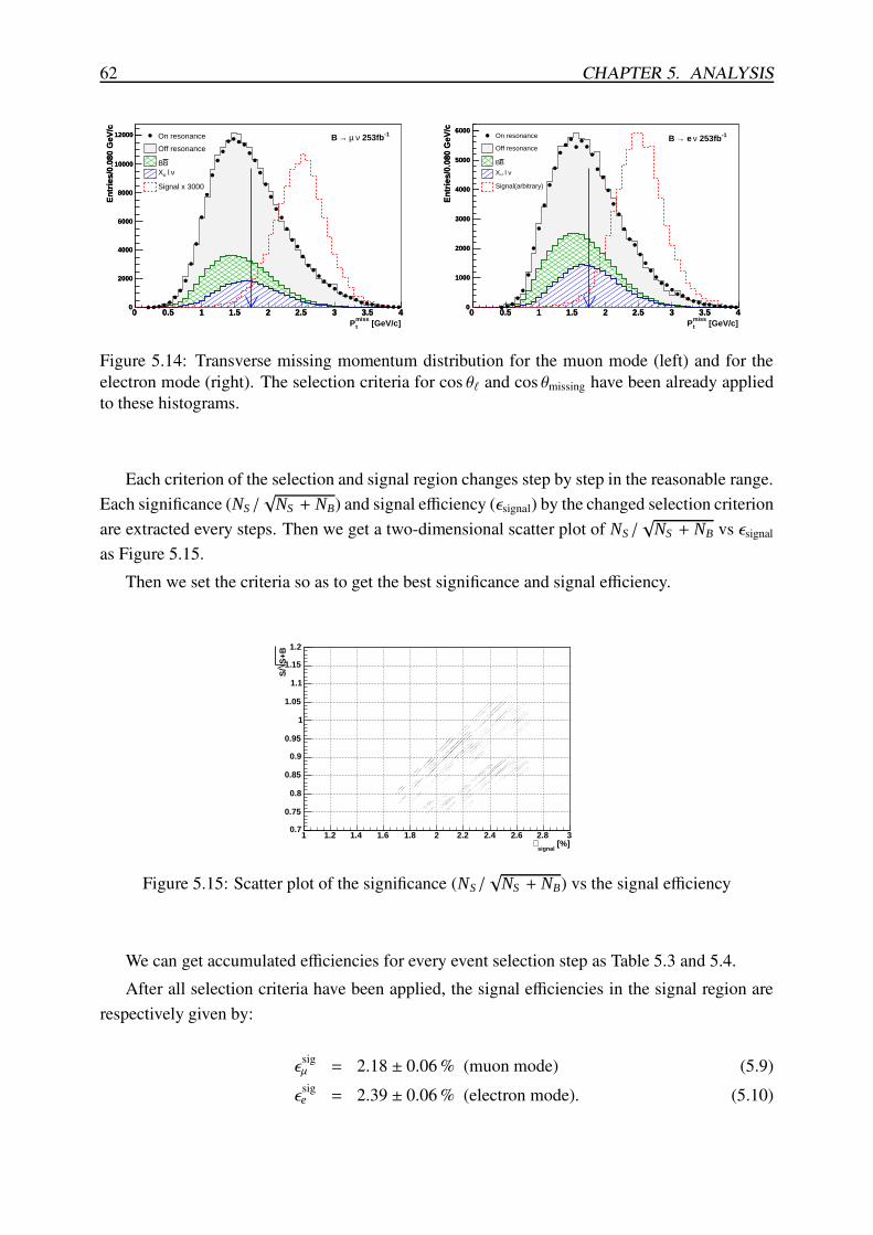
62 CHAPTER 5. ANALYSIS
0 0.5 1 1.5 2 2.5 3 3.5 4
En
trie
s/0.
080
GeV
/c
0
2000
4000
6000
8000
10000
12000
[GeV/c]misstP
0 0.5 1 1.5 2 2.5 3 3.5 4
En
trie
s/0.
080
GeV
/c
0
2000
4000
6000
8000
10000
12000 On resonance
Off resonance
BBν l uX
Signal x 3000
-1 253fbν µ →B
0 0.5 1 1.5 2 2.5 3 3.5 4
En
trie
s/0.
080
GeV
/c
0
1000
2000
3000
4000
5000
6000
[GeV/c]misstP
0 0.5 1 1.5 2 2.5 3 3.5 4
En
trie
s/0.
080
GeV
/c
0
1000
2000
3000
4000
5000
6000On resonance
Off resonance
BB
ν l uX
Signal(arbitrary)
-1 253fbν e →B
Figure 5.14: Transverse missing momentum distribution for the muon mode (left) and for theelectron mode (right). The selection criteria for cos θ` and cos θmissing have been already appliedto these histograms.
Each criterion of the selection and signal region changes step by step in the reasonable range.Each significance (NS /
√NS + NB) and signal efficiency (εsignal) by the changed selection criterion
are extracted every steps. Then we get a two-dimensional scatter plot of NS /√
NS + NB vs εsignal
as Figure 5.15.Then we set the criteria so as to get the best significance and signal efficiency.
[%]signal
∈1 1.2 1.4 1.6 1.8 2 2.2 2.4 2.6 2.8 3
S+B
S/
0.7
0.75
0.8
0.85
0.9
0.95
1
1.05
1.1
1.15
1.2
Figure 5.15: Scatter plot of the significance (NS /√
NS + NB) vs the signal efficiency
We can get accumulated efficiencies for every event selection step as Table 5.3 and 5.4.After all selection criteria have been applied, the signal efficiencies in the signal region are
respectively given by:
εsigµ = 2.18 ± 0.06 % (muon mode) (5.9)ε
sige = 2.39 ± 0.06 % (electron mode). (5.10)
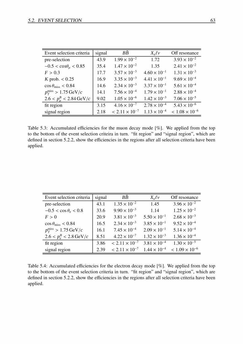
5.2. EVENT SELECTION 63
Event selection criteria signal BB Xu`ν Off resonancepre-selection 43.9 1.99 × 10⁻² 1.72 3.93 × 10⁻²
−0.5 < cosθµ < 0.85 35.4 1.47 × 10⁻² 1.35 2.41 × 10⁻²
F > 0.3 17.7 3.57 × 10⁻³ 4.60 × 10⁻¹ 1.31 × 10⁻³
K prob. < 0.25 16.9 3.35 × 10⁻³ 4.41 × 10⁻¹ 9.69 × 10⁻⁴
cos θmiss < 0.84 14.6 2.34 × 10⁻³ 3.37 × 10⁻¹ 5.61 × 10⁻⁴
pmissT > 1.75 GeV/c 14.1 7.56 × 10⁻⁴ 1.79 × 10⁻¹ 2.88 × 10⁻⁴
2.6 < pBµ < 2.84 GeV/c 9.02 1.05 × 10⁻⁶ 1.42 × 10⁻³ 7.06 × 10⁻⁵
fit region 3.15 4.16 × 10⁻⁷ 2.78 × 10⁻⁴ 5.43 × 10⁻⁶
signal region 2.18 < 2.11 × 10⁻⁷ 1.13 × 10⁻⁴ < 1.08 × 10⁻⁶
Table 5.3: Accumulated efficiencies for the muon decay mode [%]. We applied from the topto the bottom of the event selection criteira in turn. “fit region” and “signal region”, which aredefined in section 5.2.2, show the efficiencies in the regions after all selection criteria have beenapplied.
Event selection criteria signal BB Xu`ν Off resonancepre-selection 43.1 1.35 × 10⁻² 1.45 3.96 × 10⁻²
−0.5 < cos θe < 0.8 33.6 9.90 × 10⁻³ 1.14 1.25 × 10⁻²
F > 0 20.9 3.81 × 10⁻³ 5.50 × 10⁻¹ 2.68 × 10⁻³
cos θmiss < 0.84 16.5 2.34 × 10⁻³ 3.85 × 10⁻¹ 9.52 × 10⁻⁴
pmissT > 1.75 GeV/c 16.1 7.45 × 10⁻⁴ 2.09 × 10⁻¹ 5.14 × 10⁻⁴
2.6 < pBe < 2.8 GeV/c 8.51 4.22 × 10⁻⁷ 1.32 × 10⁻³ 1.36 × 10⁻⁴
fit region 3.86 < 2.11 × 10⁻⁷ 3.81 × 10⁻⁴ 1.30 × 10⁻⁵
signal region 2.39 < 2.11 × 10⁻⁷ 1.44 × 10⁻⁴ < 1.09 × 10⁻⁶
Table 5.4: Accumulated efficiencies for the electron decay mode [%]. We applied from the topto the bottom of the event selection criteria in turn. “fit region” and “signal region”, which aredefined in section 5.2.2, show the efficiencies in the regions after all selection criteria have beenapplied.
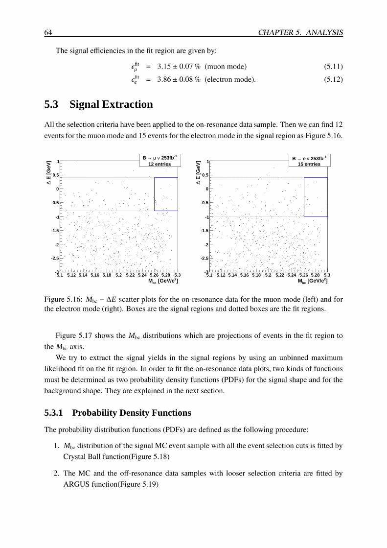
64 CHAPTER 5. ANALYSIS
The signal efficiencies in the fit region are given by:
εfitµ = 3.15 ± 0.07 % (muon mode) (5.11)εfit
e = 3.86 ± 0.08 % (electron mode). (5.12)
5.3 Signal Extraction
All the selection criteria have been applied to the on-resonance data sample. Then we can find 12events for the muon mode and 15 events for the electron mode in the signal region as Figure 5.16.
]2 [GeV/cbcM5.1 5.12 5.14 5.16 5.18 5.2 5.22 5.24 5.26 5.28 5.3
E [
GeV
]∆
-3
-2.5
-2
-1.5
-1
-0.5
0
0.5
1-1 253fbν µ →B
12 entries
]2 [GeV/cbcM5.1 5.12 5.14 5.16 5.18 5.2 5.22 5.24 5.26 5.28 5.3
E [
GeV
]∆
-3
-2.5
-2
-1.5
-1
-0.5
0
0.5
1-1 253fbν e →B
15 entries
Figure 5.16: Mbc − ∆E scatter plots for the on-resonance data for the muon mode (left) and forthe electron mode (right). Boxes are the signal regions and dotted boxes are the fit regions.
Figure 5.17 shows the Mbc distributions which are projections of events in the fit region tothe Mbc axis.
We try to extract the signal yields in the signal regions by using an unbinned maximumlikelihood fit on the fit region. In order to fit the on-resonance data plots, two kinds of functionsmust be determined as two probability density functions (PDFs) for the signal shape and for thebackground shape. They are explained in the next section.
5.3.1 Probability Density Functions
The probability distribution functions (PDFs) are defined as the following procedure:
1. Mbc distribution of the signal MC event sample with all the event selection cuts is fitted byCrystal Ball function(Figure 5.18)
2. The MC and the off-resonance data samples with looser selection criteria are fitted byARGUS function(Figure 5.19)
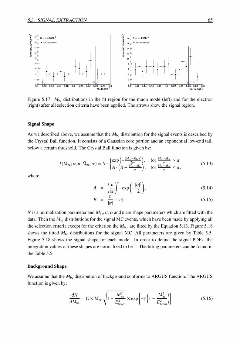
5.3. SIGNAL EXTRACTION 65
]2 [GeV/cbcM5.1 5.12 5.14 5.16 5.18 5.2 5.22 5.24 5.26 5.28 5.3
2E
ntr
ies/
0.01
0 G
eV/c
0
2
4
6
8
10
12
14
16
18
On resonance
-1 253fbν µ →B
]2 [GeV/cbcM5.1 5.12 5.14 5.16 5.18 5.2 5.22 5.24 5.26 5.28 5.3
2E
ntr
ies/
0.01
0 G
eV/c
0
2
4
6
8
10
12
14
16
18
On resonance
-1 253fbν e →B
Figure 5.17: Mbc distributions in the fit region for the muon mode (left) and for the electron(right) after all selection criteria have been applied. The arrows show the signal region.
Signal Shape
As we described above, we assume that the Mbc distribution for the signal events is described bythe Crystal Ball function. It consists of a Gaussian core portion and an exponential low-end tail,below a certain threshold. The Crystal Ball function is given by:
f (Mbc;α, n, Mbc, σ) = N ·
exp(
− (Mbc−Mbc)2
2σ2
)
, for Mbc−Mbcσ
> α
A ·(
B − Mbc−Mbcσ
)
, for Mbc−Mbcσ≤ α,
(5.13)
where
A =
(
n|α|
)n
· exp(
−|α|2
2
)
, (5.14)
B =n|α| − |α|. (5.15)
N is a normalization parameter and Mbc, σ, α and n are shape parameters which are fitted with thedata. Then the Mbc distributions for the signal MC events, which have been made by applying allthe selection criteria except for the criterion the Mbc, are fitted by the Equation 5.13. Figure 5.18shows the fitted Mbc distributions for the signal MC. All parameters are given by Table 5.5.Figure 5.18 shows the signal shape for each mode. In order to define the signal PDFs, theintegration values of these shapes are normalized to be 1. The fitting parameters can be found inthe Table 5.5.
Background Shape
We assume that the Mbc distribution of background conforms to ARGUS function. The ARGUSfunction is given by:
dNdMbc
= C × Mbc
√
1 −M2
bc
E2beam× exp
[
−ζ(
1 −M2
bc
E2beam
)]
(5.16)
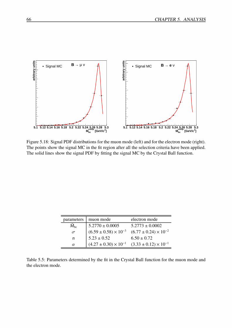
66 CHAPTER 5. ANALYSIS
]2 [GeV/ccompbcM
5.1 5.12 5.14 5.16 5.18 5.2 5.22 5.24 5.26 5.28 5.3
arb
itra
ry u
nit
s
Signal MC ν µ →B
]2 [GeV/ccompbcM
5.1 5.12 5.14 5.16 5.18 5.2 5.22 5.24 5.26 5.28 5.3ar
bit
rary
un
its
Signal MC ν e →B
Figure 5.18: Signal PDF distributions for the muon mode (left) and for the electron mode (right).The points show the signal MC in the fit region after all the selection criteria have been applied.The solid lines show the signal PDF by fitting the signal MC by the Crystal Ball function.
parameters muon mode electron modeMbc 5.2770 ± 0.0005 5.2773 ± 0.0002σ (6.59 ± 0.58) × 10−3 (6.77 ± 0.24) × 10−2
n 5.23 ± 0.52 6.50 ± 0.72α (4.27 ± 0.30) × 10−1 (3.33 ± 0.12) × 10−1
Table 5.5: Parameters determined by the fit in the Crystal Ball function for the muon mode andthe electron mode.
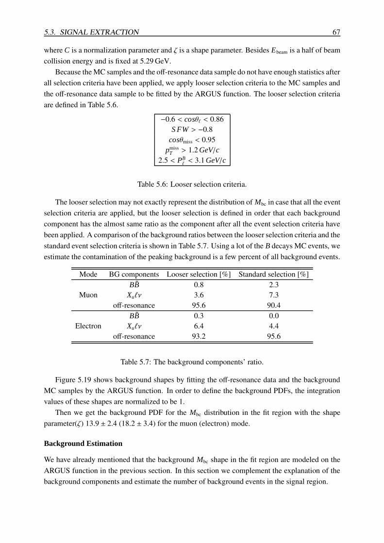
5.3. SIGNAL EXTRACTION 67
where C is a normalization parameter and ζ is a shape parameter. Besides Ebeam is a half of beamcollision energy and is fixed at 5.29 GeV.
Because the MC samples and the off-resonance data sample do not have enough statistics afterall selection criteria have been applied, we apply looser selection criteria to the MC samples andthe off-resonance data sample to be fitted by the ARGUS function. The looser selection criteriaare defined in Table 5.6.
−0.6 < cosθ` < 0.86S FW > −0.8
cosθmiss < 0.95pmiss
T > 1.2 GeV/c2.5 < PB
` < 3.1 GeV/c
Table 5.6: Looser selection criteria.
The looser selection may not exactly represent the distribution of Mbc in case that all the eventselection criteria are applied, but the looser selection is defined in order that each backgroundcomponent has the almost same ratio as the component after all the event selection criteria havebeen applied. A comparison of the background ratios between the looser selection criteria and thestandard event selection criteria is shown in Table 5.7. Using a lot of the B decays MC events, weestimate the contamination of the peaking background is a few percent of all background events.
Mode BG components Looser selection [%] Standard selection [%]
MuonBB 0.8 2.3
Xu`ν 3.6 7.3off-resonance 95.6 90.4
ElectronBB 0.3 0.0
Xu`ν 6.4 4.4off-resonance 93.2 95.6
Table 5.7: The background components’ ratio.
Figure 5.19 shows background shapes by fitting the off-resonance data and the backgroundMC samples by the ARGUS function. In order to define the background PDFs, the integrationvalues of these shapes are normalized to be 1.
Then we get the background PDF for the Mbc distribution in the fit region with the shapeparameter(ζ) 13.9 ± 2.4 (18.2 ± 3.4) for the muon (electron) mode.
Background Estimation
We have already mentioned that the background Mbc shape in the fit region are modeled on theARGUS function in the previous section. In this section we complement the explanation of thebackground components and estimate the number of background events in the signal region.
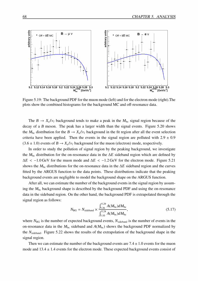
68 CHAPTER 5. ANALYSIS
]2 [GeV/ccompbcM
5.1 5.12 5.14 5.16 5.18 5.2 5.22 5.24 5.26 5.28 5.3
arb
itra
ry u
nit
s
MCBOff + Bν µ →B
]2 [GeV/ccompbcM
5.1 5.12 5.14 5.16 5.18 5.2 5.22 5.24 5.26 5.28 5.3
arb
itra
ry u
nit
s
MCBOff + B ν e →B
Figure 5.19: The background PDF for the muon mode (left) and for the electron mode (right).Theplots show the combined histograms for the background MC and off-resonance data.
The B → Xu`ν` background tends to make a peak in the Mbc signal region because of thedecay of a B meson. The peak has a larger width than the signal events. Figure 5.20 showsthe Mbc distribution for the B → Xu`ν` background in the fit region after all the event selectioncriteria have been applied. Then the events in the signal region are polluted with 2.9 ± 0.9(3.6 ± 1.0) events of B→ Xu`ν` background for the muon (electron) mode, respectively.
In order to study the pollution of signal region by the peaking background, we investigatethe Mbc distribution for the on-resonance data in the ∆E sideband region which are defined by∆E < −1.0 GeV for the muon mode and ∆E < −1.2 GeV for the electron mode. Figure 5.21shows the Mbc distributions for the on-resonance data in the ∆E sideband region and the curvesfitted by the ARGUS function to the data points. These distributions indicate that the peakingbackground events are negligible to model the background shape on the ARGUS function.
After all, we can estimate the number of the background events in the signal region by assum-ing the Mbc background shape is described by the background PDF and using the on-resonancedata in the sideband region. On the other hand, the background PDF is extrapolated through thesignal region as follows:
NBG = Nsideband ×∫ 5.29
5.26 A(Mbc)dMbc∫ 5.24
5.10 A(Mbc)dMbc
, (5.17)
where NBG is the number of expected background events, Nsideband is the number of events in theon-resonance data in the Mbc sideband and A(Mbc) shows the background PDF normalized bythe Nsideband. Figure 5.22 shows the results of the extrapolation of the background shape in thesignal region.
Then we can estimate the number of the background events are 7.4± 1.0 events for the muonmode and 13.4 ± 1.4 events for the electron mode. These expected background events consist of
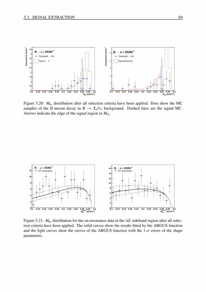
5.3. SIGNAL EXTRACTION 69
]2 [GeV/cbcM5.1 5.12 5.14 5.16 5.18 5.2 5.22 5.24 5.26 5.28 5.3
2E
ntr
ies/
0.01
GeV
/c
0
0.5
1
1.5
2
2.5
3
3.5
4
4.5
)ν Xl→Peaking(B
Signal x 3
-1 253fbν µ →B
]2 [GeV/cbcM5.1 5.12 5.14 5.16 5.18 5.2 5.22 5.24 5.26 5.28 5.3
2E
ntr
ies/
0.01
GeV
/c
0
1
2
3
4
5
)ν Xl→Peaking(B
Signal(arbitrary)
-1 253fbν e →B
Figure 5.20: Mbc distribution after all selection criteria have been applied. Dots show the MCsamples of the B meson decay in B → Xu`ν` background. Dashed lines are the signal MC.Arrows indicate the edge of the signal region in Mbc.
]2 [GeV/ccompbcM
5.1 5.12 5.14 5.16 5.18 5.2 5.22 5.24 5.26 5.28 5.30
2
4
6
8
10
12 On resonance
-1 253fbν µ →B
]2 [GeV/ccompbcM
5.1 5.12 5.14 5.16 5.18 5.2 5.22 5.24 5.26 5.28 5.30
2
4
6
8
10
12
14
16On resonance
-1 253fbν e →B
Figure 5.21: Mbc distribution for the on-resonance data in the ∆E sideband region after all selec-tion criteria have been applied. The solid curves show the results fitted by the ARGUS functionand the light curves show the curves of the ARGUS function with the 1-σ errors of the shapeparameters.
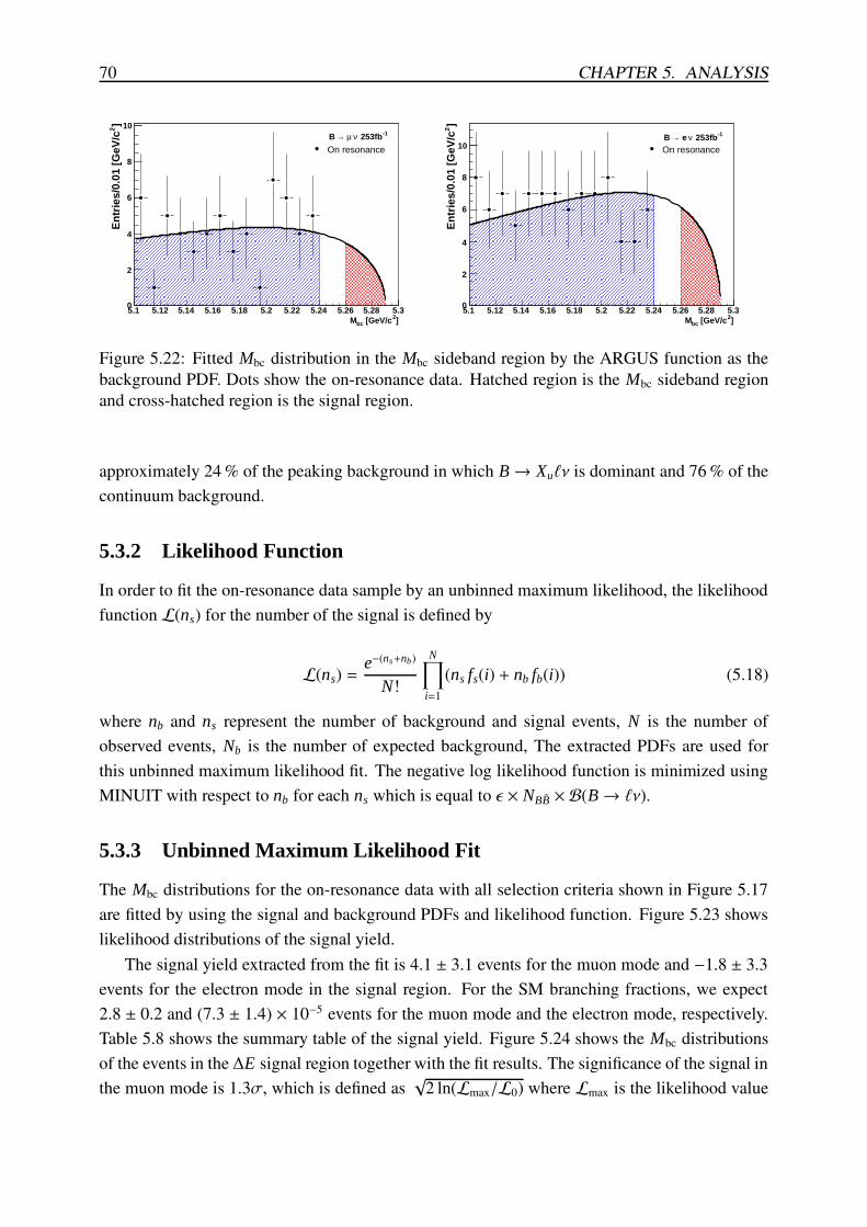
70 CHAPTER 5. ANALYSIS
]2 [GeV/cbcM5.1 5.12 5.14 5.16 5.18 5.2 5.22 5.24 5.26 5.28 5.3
]2
En
trie
s/0.
01 [
GeV
/c
0
2
4
6
8
10
On resonance
-1 253fbν µ →B
]2 [GeV/cbcM5.1 5.12 5.14 5.16 5.18 5.2 5.22 5.24 5.26 5.28 5.3
]2
En
trie
s/0.
01 [
GeV
/c
0
2
4
6
8
10 On resonance
-1 253fbν e →B
Figure 5.22: Fitted Mbc distribution in the Mbc sideband region by the ARGUS function as thebackground PDF. Dots show the on-resonance data. Hatched region is the Mbc sideband regionand cross-hatched region is the signal region.
approximately 24 % of the peaking background in which B→ Xu`ν is dominant and 76 % of thecontinuum background.
5.3.2 Likelihood Function
In order to fit the on-resonance data sample by an unbinned maximum likelihood, the likelihoodfunction L(ns) for the number of the signal is defined by
L(ns) =e−(ns+nb)
N!
N∏
i=1(ns fs(i) + nb fb(i)) (5.18)
where nb and ns represent the number of background and signal events, N is the number ofobserved events, Nb is the number of expected background, The extracted PDFs are used forthis unbinned maximum likelihood fit. The negative log likelihood function is minimized usingMINUIT with respect to nb for each ns which is equal to ε × NBB × B(B→ `ν).
5.3.3 Unbinned Maximum Likelihood Fit
The Mbc distributions for the on-resonance data with all selection criteria shown in Figure 5.17are fitted by using the signal and background PDFs and likelihood function. Figure 5.23 showslikelihood distributions of the signal yield.
The signal yield extracted from the fit is 4.1 ± 3.1 events for the muon mode and −1.8 ± 3.3events for the electron mode in the signal region. For the SM branching fractions, we expect2.8 ± 0.2 and (7.3 ± 1.4) × 10−5 events for the muon mode and the electron mode, respectively.Table 5.8 shows the summary table of the signal yield. Figure 5.24 shows the Mbc distributionsof the events in the ∆E signal region together with the fit results. The significance of the signal inthe muon mode is 1.3σ, which is defined as
√2 ln(Lmax/L0) where Lmax is the likelihood value
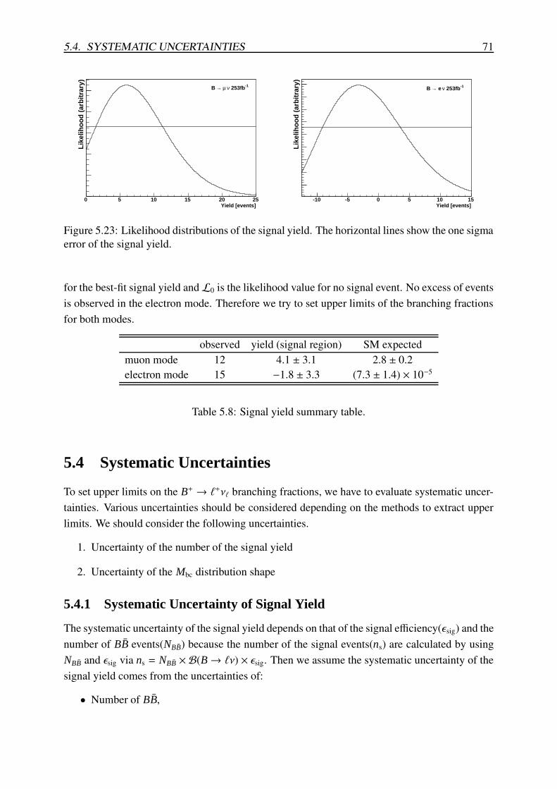
5.4. SYSTEMATIC UNCERTAINTIES 71
Yield [events]0 5 10 15 20 25
Lik
elih
oo
d (
arb
itra
ry)
-1 253fbν µ →B
Yield [events]-10 -5 0 5 10 15
Lik
elih
oo
d (
arb
itra
ry)
-1 253fbν e →B
Figure 5.23: Likelihood distributions of the signal yield. The horizontal lines show the one sigmaerror of the signal yield.
for the best-fit signal yield andL0 is the likelihood value for no signal event. No excess of eventsis observed in the electron mode. Therefore we try to set upper limits of the branching fractionsfor both modes.
observed yield (signal region) SM expectedmuon mode 12 4.1 ± 3.1 2.8 ± 0.2electron mode 15 −1.8 ± 3.3 (7.3 ± 1.4) × 10−5
Table 5.8: Signal yield summary table.
5.4 Systematic Uncertainties
To set upper limits on the B+ → `+ν` branching fractions, we have to evaluate systematic uncer-tainties. Various uncertainties should be considered depending on the methods to extract upperlimits. We should consider the following uncertainties.
1. Uncertainty of the number of the signal yield
2. Uncertainty of the Mbc distribution shape
5.4.1 Systematic Uncertainty of Signal Yield
The systematic uncertainty of the signal yield depends on that of the signal efficiency(εsig) and thenumber of BB events(NBB) because the number of the signal events(ns) are calculated by usingNBB and εsig via ns = NBB × B(B→ `ν) × εsig. Then we assume the systematic uncertainty of thesignal yield comes from the uncertainties of:
• Number of BB,
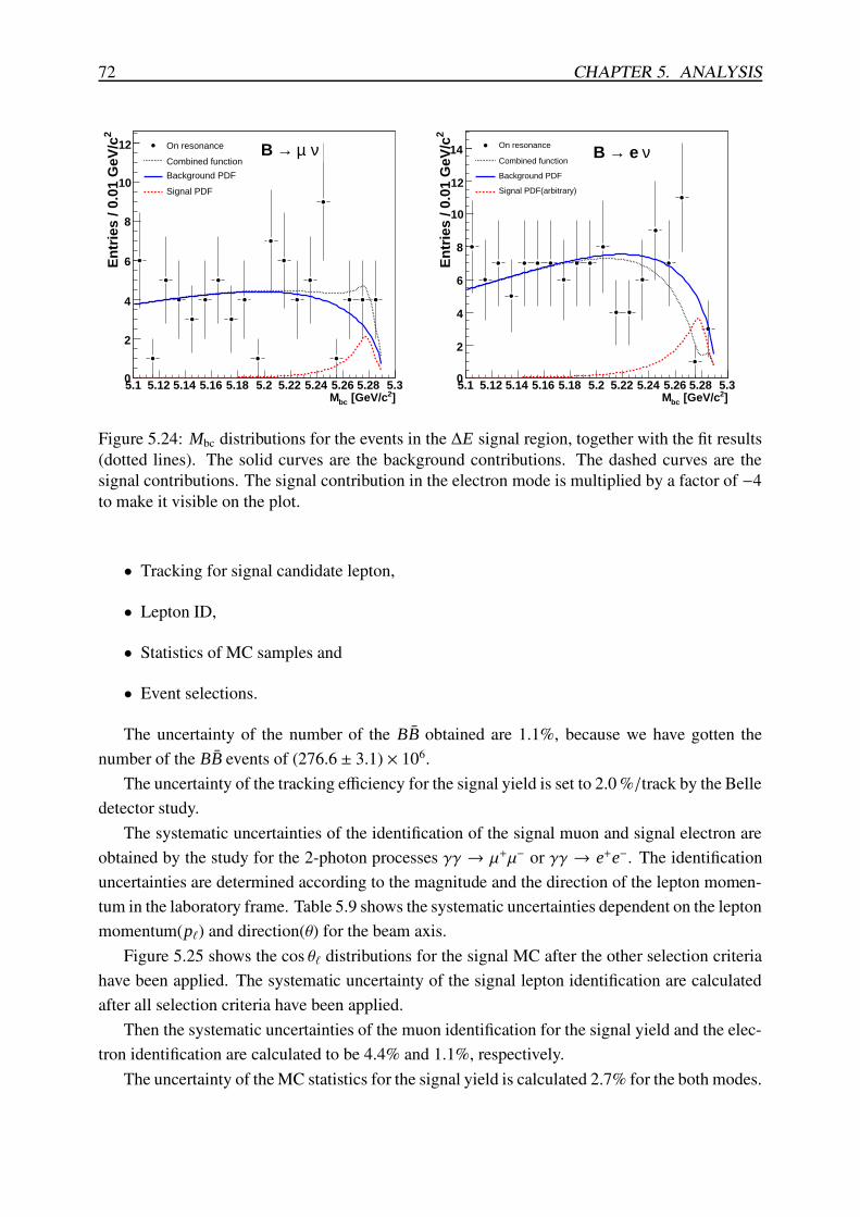
72 CHAPTER 5. ANALYSIS
]2 [GeV/cbcM5.1 5.12 5.14 5.16 5.18 5.2 5.22 5.24 5.26 5.28 5.3
2E
ntr
ies
/ 0.0
1 G
eV/c
0
2
4
6
8
10
12 On resonance
Combined function
Background PDF
Signal PDF
ν µ →B
]2 [GeV/cbcM5.1 5.12 5.14 5.16 5.18 5.2 5.22 5.24 5.26 5.28 5.3
2E
ntr
ies
/ 0.0
1 G
eV/c
0
2
4
6
8
10
12
14 On resonance
Combined function
Background PDF
Signal PDF(arbitrary)
ν e →B
Figure 5.24: Mbc distributions for the events in the ∆E signal region, together with the fit results(dotted lines). The solid curves are the background contributions. The dashed curves are thesignal contributions. The signal contribution in the electron mode is multiplied by a factor of −4to make it visible on the plot.
• Tracking for signal candidate lepton,
• Lepton ID,
• Statistics of MC samples and
• Event selections.
The uncertainty of the number of the BB obtained are 1.1%, because we have gotten thenumber of the BB events of (276.6 ± 3.1) × 106.
The uncertainty of the tracking efficiency for the signal yield is set to 2.0 %/track by the Belledetector study.
The systematic uncertainties of the identification of the signal muon and signal electron areobtained by the study for the 2-photon processes γγ → µ+µ− or γγ → e+e−. The identificationuncertainties are determined according to the magnitude and the direction of the lepton momen-tum in the laboratory frame. Table 5.9 shows the systematic uncertainties dependent on the leptonmomentum(p`) and direction(θ) for the beam axis.
Figure 5.25 shows the cos θ` distributions for the signal MC after the other selection criteriahave been applied. The systematic uncertainty of the signal lepton identification are calculatedafter all selection criteria have been applied.
Then the systematic uncertainties of the muon identification for the signal yield and the elec-tron identification are calculated to be 4.4% and 1.1%, respectively.
The uncertainty of the MC statistics for the signal yield is calculated 2.7% for the both modes.
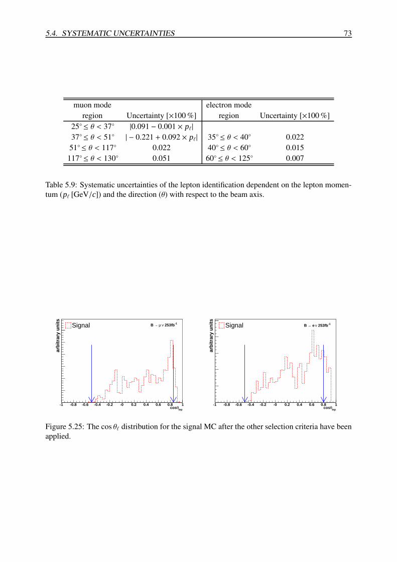
5.4. SYSTEMATIC UNCERTAINTIES 73
muon mode electron moderegion Uncertainty [×100 %] region Uncertainty [×100 %]
25◦≤ θ < 37◦ |0.091 − 0.001 × p` |37◦≤ θ < 51◦ | − 0.221 + 0.092 × p`| 35◦≤ θ < 40◦ 0.02251◦≤ θ < 117◦ 0.022 40◦≤ θ < 60◦ 0.015
117◦≤ θ < 130◦ 0.051 60◦≤ θ < 125◦ 0.007
Table 5.9: Systematic uncertainties of the lepton identification dependent on the lepton momen-tum (p` [GeV/c]) and the direction (θ) with respect to the beam axis.
lepθcos-1 -0.8 -0.6 -0.4 -0.2 -0 0.2 0.4 0.6 0.8 1
arb
itra
ry u
nit
s
Signal -1 253fbν µ →B
lepθcos-1 -0.8 -0.6 -0.4 -0.2 -0 0.2 0.4 0.6 0.8 1
arb
itra
ry u
nit
s
Signal -1 253fbν e →B
Figure 5.25: The cos θ` distribution for the signal MC after the other selection criteria have beenapplied.
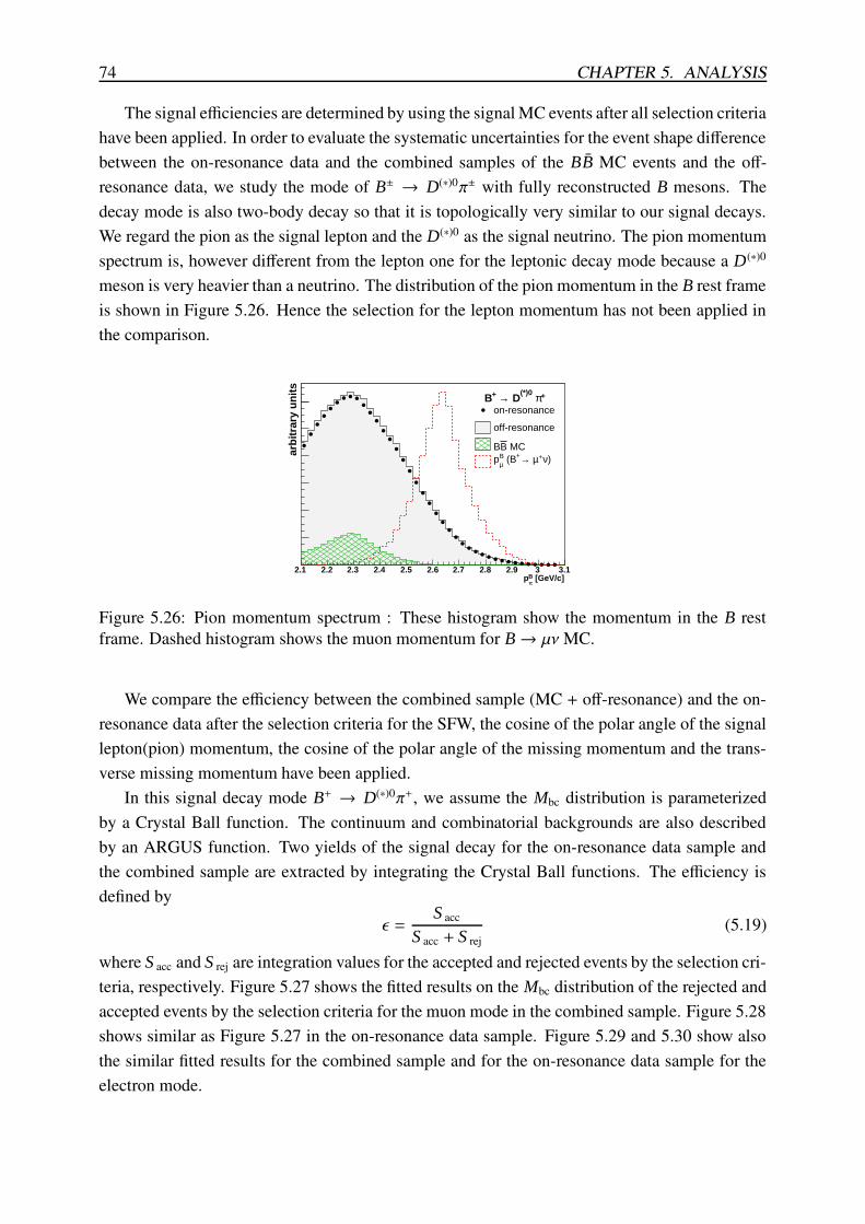
74 CHAPTER 5. ANALYSIS
The signal efficiencies are determined by using the signal MC events after all selection criteriahave been applied. In order to evaluate the systematic uncertainties for the event shape differencebetween the on-resonance data and the combined samples of the BB MC events and the off-resonance data, we study the mode of B± → D(∗)0π± with fully reconstructed B mesons. Thedecay mode is also two-body decay so that it is topologically very similar to our signal decays.We regard the pion as the signal lepton and the D(∗)0 as the signal neutrino. The pion momentumspectrum is, however different from the lepton one for the leptonic decay mode because a D(∗)0
meson is very heavier than a neutrino. The distribution of the pion momentum in the B rest frameis shown in Figure 5.26. Hence the selection for the lepton momentum has not been applied inthe comparison.
[GeV/c]Bπ
p2.1 2.2 2.3 2.4 2.5 2.6 2.7 2.8 2.9 3 3.1
arb
itra
ry u
nit
s
on-resonance
off-resonance
MCBB)ν+µ →+ (BB
µp
+π (*)0 D→ +B
Figure 5.26: Pion momentum spectrum : These histogram show the momentum in the B restframe. Dashed histogram shows the muon momentum for B→ µν MC.
We compare the efficiency between the combined sample (MC + off-resonance) and the on-resonance data after the selection criteria for the SFW, the cosine of the polar angle of the signallepton(pion) momentum, the cosine of the polar angle of the missing momentum and the trans-verse missing momentum have been applied.
In this signal decay mode B+ → D(∗)0π+, we assume the Mbc distribution is parameterizedby a Crystal Ball function. The continuum and combinatorial backgrounds are also describedby an ARGUS function. Two yields of the signal decay for the on-resonance data sample andthe combined sample are extracted by integrating the Crystal Ball functions. The efficiency isdefined by
ε =S acc
S acc + S rej(5.19)
where S acc and S rej are integration values for the accepted and rejected events by the selection cri-teria, respectively. Figure 5.27 shows the fitted results on the Mbc distribution of the rejected andaccepted events by the selection criteria for the muon mode in the combined sample. Figure 5.28shows similar as Figure 5.27 in the on-resonance data sample. Figure 5.29 and 5.30 show alsothe similar fitted results for the combined sample and for the on-resonance data sample for theelectron mode.
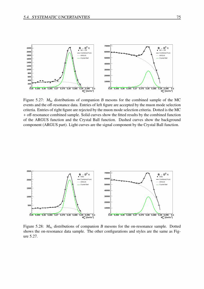
5.4. SYSTEMATIC UNCERTAINTIES 75
]2 [GeV/cπDbcM
5.25 5.255 5.26 5.265 5.27 5.275 5.28 5.285 5.29 5.295 5.30
200
400
600
800
1000
1200
1400
1600
1800
2000
2200MC + Off
Combined Func
ARGUS
Crystal Ball
π 0 D→B
]2 [GeV/cπDbcM
5.25 5.255 5.26 5.265 5.27 5.275 5.28 5.285 5.29 5.295 5.30
10000
20000
30000
40000
50000
60000
70000
MC + Off
Combined Func
ARGUS
Crystal Ball
π 0 D→B
Figure 5.27: Mbc distributions of companion B mesons for the combined sample of the MCevents and the off-resonance data. Entries of left figure are accepted by the muon mode selectioncriteria. Entries of right figure are rejected by the muon mode selection criteria. Dotted is the MC+ off-resonance combined sample. Solid curves show the fitted results by the combined functionof the ARGUS function and the Crystal Ball function. Dashed curves show the backgroundcomponent (ARGUS part). Light curves are the signal component by the Crystal Ball function.
]2 [GeV/cπDbcM
5.25 5.255 5.26 5.265 5.27 5.275 5.28 5.285 5.29 5.295 5.30
500
1000
1500
2000
2500
Data
Combined Func
ARGUS
Crystal Ball
π 0 D→B
]2 [GeV/cπDbcM
5.25 5.255 5.26 5.265 5.27 5.275 5.28 5.285 5.29 5.295 5.30
10000
20000
30000
40000
50000
60000
70000
Data
Combined Func
ARGUS
Crystal Ball
π 0 D→B
Figure 5.28: Mbc distributions of companion B mesons for the on-resonance sample. Dottedshows the on-resonance data sample. The other configurations and styles are the same as Fig-ure 5.27.
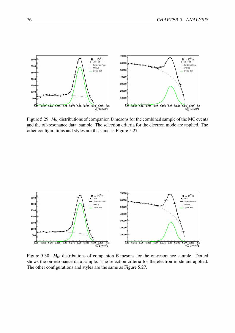
76 CHAPTER 5. ANALYSIS
]2 [GeV/cπDbcM
5.25 5.255 5.26 5.265 5.27 5.275 5.28 5.285 5.29 5.295 5.30
500
1000
1500
2000
2500
3000
3500MC + Off
Combined Func
ARGUS
Crystal Ball
π 0 D→B
]2 [GeV/cπDbcM
5.25 5.255 5.26 5.265 5.27 5.275 5.28 5.285 5.29 5.295 5.30
10000
20000
30000
40000
50000
60000
70000
MC + Off
Combined Func
ARGUS
Crystal Ball
π 0 D→B
Figure 5.29: Mbc distributions of companion B mesons for the combined sample of the MC eventsand the off-resonance data. sample. The selection criteria for the electron mode are applied. Theother configurations and styles are the same as Figure 5.27.
]2 [GeV/cπDbcM
5.25 5.255 5.26 5.265 5.27 5.275 5.28 5.285 5.29 5.295 5.30
500
1000
1500
2000
2500
3000
3500 Data
Combined Func
ARGUS
Crystal Ball
π 0 D→B
]2 [GeV/cπDbcM
5.25 5.255 5.26 5.265 5.27 5.275 5.28 5.285 5.29 5.295 5.30
10000
20000
30000
40000
50000
60000
70000
Data
Combined Func
ARGUS
Crystal Ball
π 0 D→B
Figure 5.30: Mbc distributions of companion B mesons for the on-resonance sample. Dottedshows the on-resonance data sample. The selection criteria for the electron mode are applied.The other configurations and styles are the same as Figure 5.27.
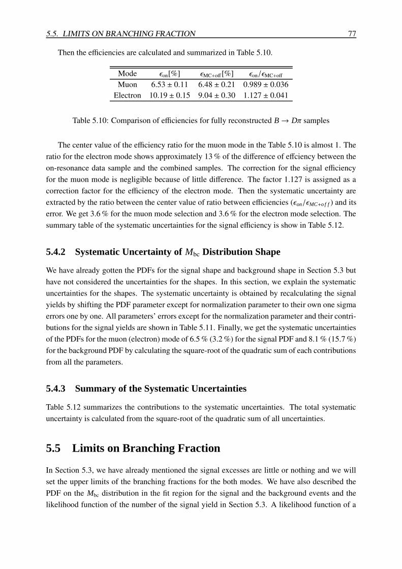
5.5. LIMITS ON BRANCHING FRACTION 77
Then the efficiencies are calculated and summarized in Table 5.10.
Mode εon[%] εMC+off[%] εon/εMC+off
Muon 6.53 ± 0.11 6.48 ± 0.21 0.989 ± 0.036Electron 10.19 ± 0.15 9.04 ± 0.30 1.127 ± 0.041
Table 5.10: Comparison of efficiencies for fully reconstructed B→ Dπ samples
The center value of the efficiency ratio for the muon mode in the Table 5.10 is almost 1. Theratio for the electron mode shows approximately 13 % of the difference of effciency between theon-resonance data sample and the combined samples. The correction for the signal efficiencyfor the muon mode is negligible because of little difference. The factor 1.127 is assigned as acorrection factor for the efficiency of the electron mode. Then the systematic uncertainty areextracted by the ratio between the center value of ratio between efficiencies (εon/εMC+o f f ) and itserror. We get 3.6 % for the muon mode selection and 3.6 % for the electron mode selection. Thesummary table of the systematic uncertainties for the signal efficiency is show in Table 5.12.
5.4.2 Systematic Uncertainty of Mbc Distribution Shape
We have already gotten the PDFs for the signal shape and background shape in Section 5.3 buthave not considered the uncertainties for the shapes. In this section, we explain the systematicuncertainties for the shapes. The systematic uncertainty is obtained by recalculating the signalyields by shifting the PDF parameter except for normalization parameter to their own one sigmaerrors one by one. All parameters’ errors except for the normalization parameter and their contri-butions for the signal yields are shown in Table 5.11. Finally, we get the systematic uncertaintiesof the PDFs for the muon (electron) mode of 6.5 % (3.2 %) for the signal PDF and 8.1 % (15.7 %)for the background PDF by calculating the square-root of the quadratic sum of each contributionsfrom all the parameters.
5.4.3 Summary of the Systematic Uncertainties
Table 5.12 summarizes the contributions to the systematic uncertainties. The total systematicuncertainty is calculated from the square-root of the quadratic sum of all uncertainties.
5.5 Limits on Branching Fraction
In Section 5.3, we have already mentioned the signal excesses are little or nothing and we willset the upper limits of the branching fractions for the both modes. We have also described thePDF on the Mbc distribution in the fit region for the signal and the background events and thelikelihood function of the number of the signal yield in Section 5.3. A likelihood function of a
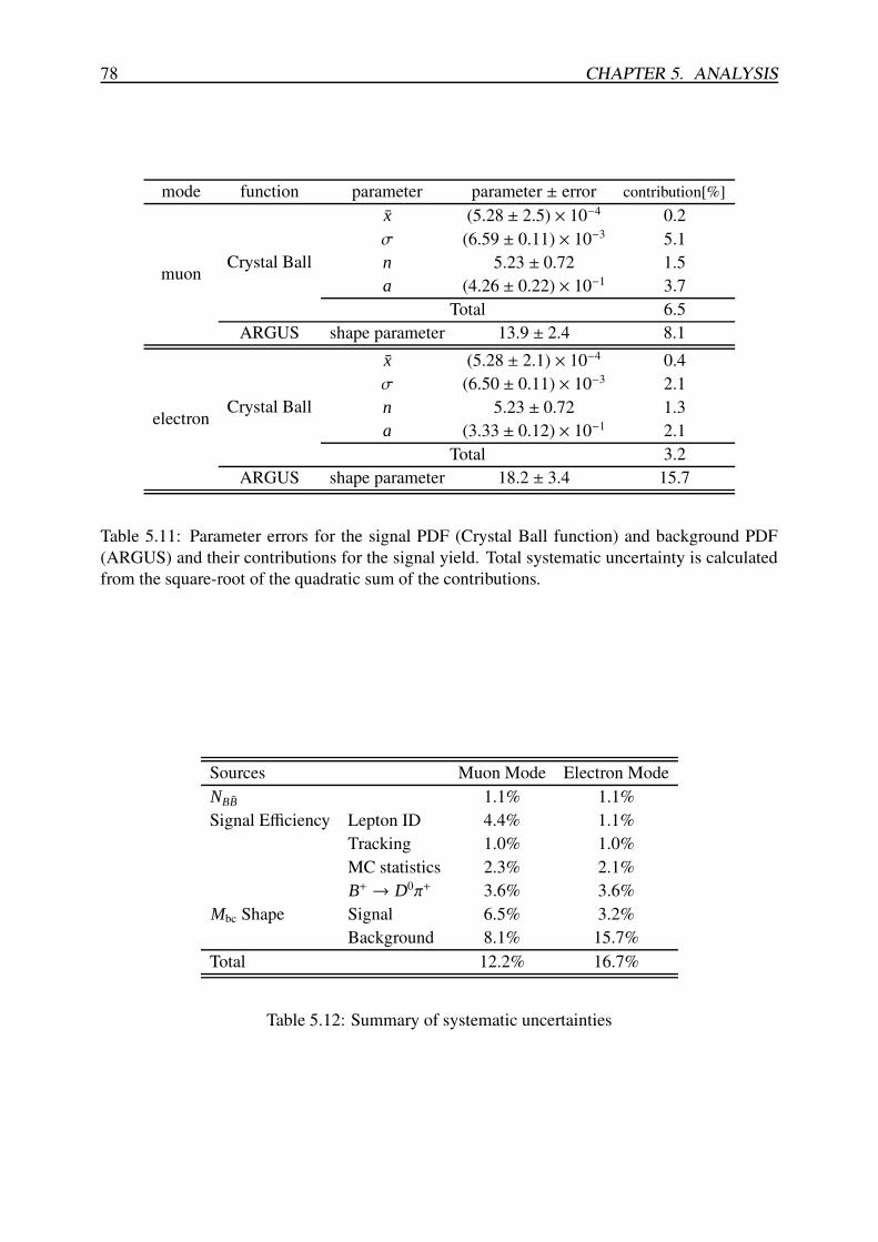
78 CHAPTER 5. ANALYSIS
mode function parameter parameter ± error contribution[%]
muon Crystal Ball
x (5.28 ± 2.5) × 10−4 0.2σ (6.59 ± 0.11) × 10−3 5.1n 5.23 ± 0.72 1.5a (4.26 ± 0.22) × 10−1 3.7
Total 6.5ARGUS shape parameter 13.9 ± 2.4 8.1
electron Crystal Ball
x (5.28 ± 2.1) × 10−4 0.4σ (6.50 ± 0.11) × 10−3 2.1n 5.23 ± 0.72 1.3a (3.33 ± 0.12) × 10−1 2.1
Total 3.2ARGUS shape parameter 18.2 ± 3.4 15.7
Table 5.11: Parameter errors for the signal PDF (Crystal Ball function) and background PDF(ARGUS) and their contributions for the signal yield. Total systematic uncertainty is calculatedfrom the square-root of the quadratic sum of the contributions.
Sources Muon Mode Electron ModeNBB 1.1% 1.1%Signal Efficiency Lepton ID 4.4% 1.1%
Tracking 1.0% 1.0%MC statistics 2.3% 2.1%B+ → D0π+ 3.6% 3.6%
Mbc Shape Signal 6.5% 3.2%Background 8.1% 15.7%
Total 12.2% 16.7%
Table 5.12: Summary of systematic uncertainties
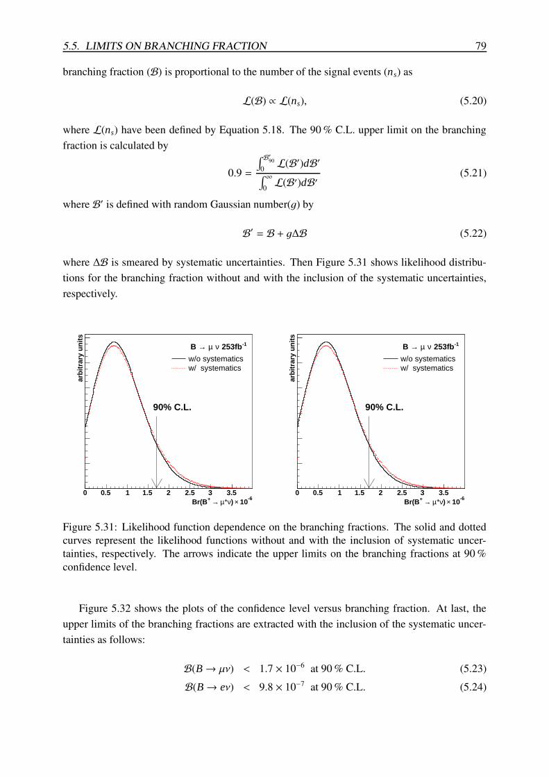
5.5. LIMITS ON BRANCHING FRACTION 79
branching fraction (B) is proportional to the number of the signal events (ns) as
L(B) ∝ L(ns), (5.20)
where L(ns) have been defined by Equation 5.18. The 90 % C.L. upper limit on the branchingfraction is calculated by
0.9 =
∫ B′900 L(B′)dB′∫ ∞
0 L(B′)dB′(5.21)
where B′ is defined with random Gaussian number(1) by
B′ = B + 1∆B (5.22)
where ∆B is smeared by systematic uncertainties. Then Figure 5.31 shows likelihood distribu-tions for the branching fraction without and with the inclusion of the systematic uncertainties,respectively.
-6 10×) ν+µ → +Br(B
0 0.5 1 1.5 2 2.5 3 3.5
arb
itra
ry u
nit
s
w/o systematicsw/ systematics
-1 253fbν µ →B
90% C.L.
-6 10×) ν+µ → +Br(B
0 0.5 1 1.5 2 2.5 3 3.5
arb
itra
ry u
nit
s
w/o systematicsw/ systematics
-1 253fbν µ →B
90% C.L.
Figure 5.31: Likelihood function dependence on the branching fractions. The solid and dottedcurves represent the likelihood functions without and with the inclusion of systematic uncer-tainties, respectively. The arrows indicate the upper limits on the branching fractions at 90 %confidence level.
Figure 5.32 shows the plots of the confidence level versus branching fraction. At last, theupper limits of the branching fractions are extracted with the inclusion of the systematic uncer-tainties as follows:
B(B→ µν) < 1.7 × 10⁻⁶ at 90 % C.L. (5.23)B(B→ eν) < 9.8 × 10⁻⁷ at 90 % C.L. (5.24)
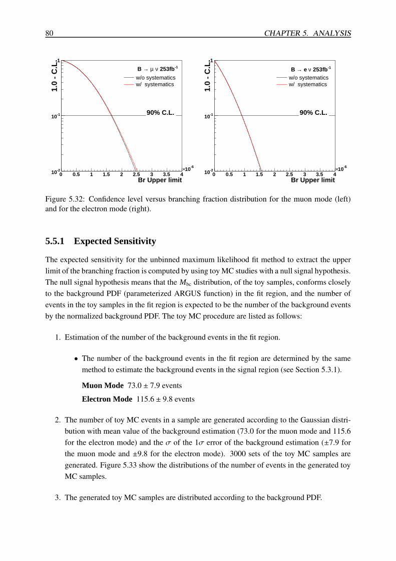
80 CHAPTER 5. ANALYSIS
Br Upper limit0 0.5 1 1.5 2 2.5 3 3.5 4
-610×
1.0
- C
.L.
-210
-110
1
w/o systematicsw/ systematics
-1 253fbν µ →B
90% C.L.
Br Upper limit0 0.5 1 1.5 2 2.5 3 3.5 4
-610×
1.0
- C
.L.
-210
-110
1
w/o systematicsw/ systematics
-1 253fbν e →B
90% C.L.
Figure 5.32: Confidence level versus branching fraction distribution for the muon mode (left)and for the electron mode (right).
5.5.1 Expected Sensitivity
The expected sensitivity for the unbinned maximum likelihood fit method to extract the upperlimit of the branching fraction is computed by using toy MC studies with a null signal hypothesis.The null signal hypothesis means that the Mbc distribution, of the toy samples, conforms closelyto the background PDF (parameterized ARGUS function) in the fit region, and the number ofevents in the toy samples in the fit region is expected to be the number of the background eventsby the normalized background PDF. The toy MC procedure are listed as follows:
1. Estimation of the number of the background events in the fit region.
• The number of the background events in the fit region are determined by the samemethod to estimate the background events in the signal region (see Section 5.3.1).
Muon Mode 73.0 ± 7.9 eventsElectron Mode 115.6 ± 9.8 events
2. The number of toy MC events in a sample are generated according to the Gaussian distri-bution with mean value of the background estimation (73.0 for the muon mode and 115.6for the electron mode) and the σ of the 1σ error of the background estimation (±7.9 forthe muon mode and ±9.8 for the electron mode). 3000 sets of the toy MC samples aregenerated. Figure 5.33 show the distributions of the number of events in the generated toyMC samples.
3. The generated toy MC samples are distributed according to the background PDF.
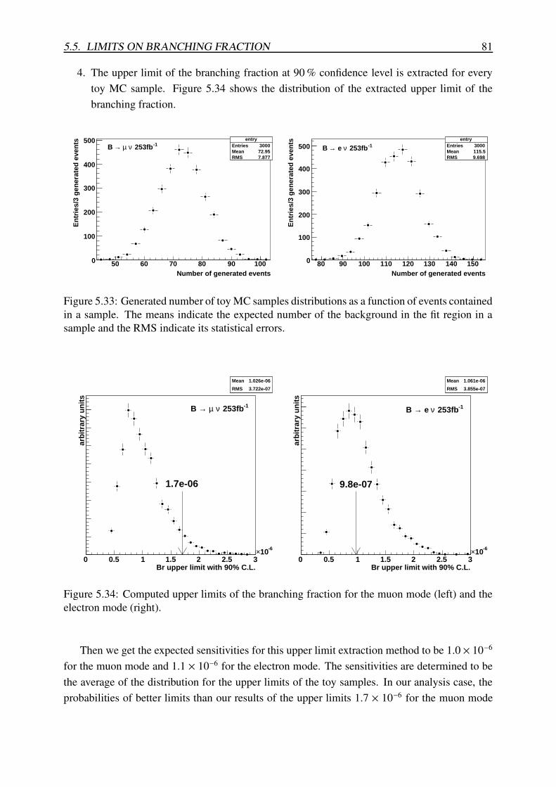
5.5. LIMITS ON BRANCHING FRACTION 81
4. The upper limit of the branching fraction at 90 % confidence level is extracted for everytoy MC sample. Figure 5.34 shows the distribution of the extracted upper limit of thebranching fraction.
entryEntries 3000Mean 72.95RMS 7.877
Number of generated events50 60 70 80 90 100
En
trie
s/3
gen
erat
ed e
ven
ts
0
100
200
300
400
500 entryEntries 3000Mean 72.95RMS 7.877
-1 253fbν µ →B entry
Entries 3000Mean 115.5RMS 9.698
Number of generated events80 90 100 110 120 130 140 150
En
trie
s/3
gen
erat
ed e
ven
ts
0
100
200
300
400
500entry
Entries 3000Mean 115.5RMS 9.698
-1 253fbν e →B
Figure 5.33: Generated number of toy MC samples distributions as a function of events containedin a sample. The means indicate the expected number of the background in the fit region in asample and the RMS indicate its statistical errors.
Mean 1.026e-06
RMS 3.722e-07
Br upper limit with 90% C.L.0 0.5 1 1.5 2 2.5 3
-610×
arb
itra
ry u
nit
s
Mean 1.026e-06
RMS 3.722e-07
-1 253fbν µ →B
1.7e-06
Mean 1.061e-06
RMS 3.855e-07
Br upper limit with 90% C.L.0 0.5 1 1.5 2 2.5 3
-610×
arb
itra
ry u
nit
s
Mean 1.061e-06
RMS 3.855e-07
-1 253fbν e →B
9.8e-07
Figure 5.34: Computed upper limits of the branching fraction for the muon mode (left) and theelectron mode (right).
Then we get the expected sensitivities for this upper limit extraction method to be 1.0 × 10⁻⁶
for the muon mode and 1.1 × 10⁻⁶ for the electron mode. The sensitivities are determined to bethe average of the distribution for the upper limits of the toy samples. In our analysis case, theprobabilities of better limits than our results of the upper limits 1.7 × 10⁻⁶ for the muon mode

82 CHAPTER 5. ANALYSIS
and 9.8 × 10⁻⁷ for the electron mode, are 94.3 % for the muon mode and 50.3 % for the electronmode, respectively. Our toy study indicate our result for the muon mode rare case.
Chapter 6
Conclusion and Discussion
6.1 Conclusion
We have searched for the purely leptonic decays B+ → µ+νµ and B+ → e+νe using the 253 fb−1
data collected by the Belle detector at the KEKB e+e− asymmetric-energy collider. We havefound no evidence of the signal in either decay mode. We set upper limits on the branchingfractions:
B(B+ → µ+νµ) < 1.7 × 10⁻⁶, (6.1)B(B+ → e+νe) < 9.8 × 10⁻⁷ (6.2)
at 90 % confidence level.In the following section, we discuss the result of the upper limits of the branching fraction
with other upper limits.
6.2 Discussion
Obtained upper limits are the most stringent to date and improve the previous published lim-its [26, 27] by a factor of 4 for B+ → µ+νµ and 15 for B+ → e+νe. Figure 6.1 shows the upperlimits’ changes and the branching fraction expected by the SM. Our results are consistent withthe SM predictions.
The B meson decay constant, fB can be only measured by the leptonic B meson decays.However we can not set the branching fractions but the upper limits. Therefore we just introducethe recent result of the fB by first direct measurement B+ → τ+ντ [25]. The fB has been also setin the paper as follows:
fB = 0.229+0.036−0.031(stat)+0.034
−0.037(syst) GeV. (6.3)
In our study, the signal yields are extracted as 4.1 ± 3.1 for the muon mode and −1.8 ±3.3 for the electron mode and the significance of the signal yield for the muon mode is 1.3σ.(see Section 5.3). For the muon mode, especially the ratio of the error for the signal yield isapproximately 75 %. Because this error of the signal yield dominantly come from data statistics,
83
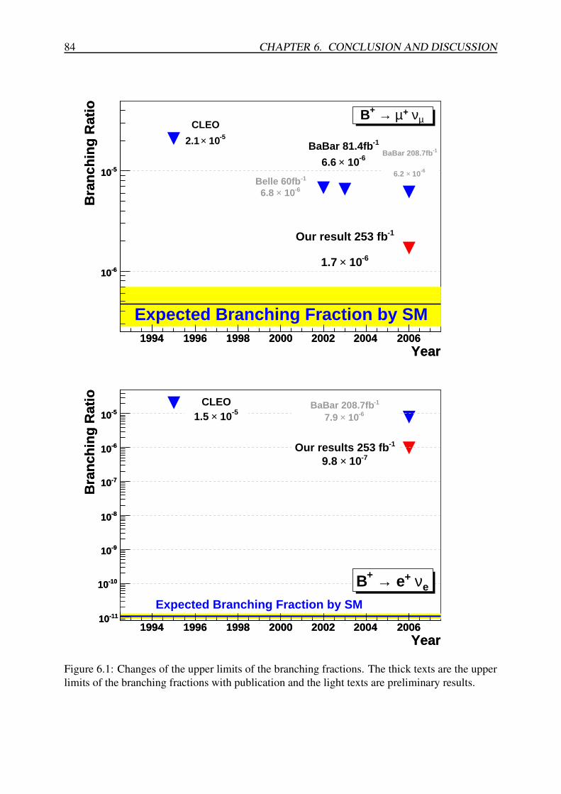
84 CHAPTER 6. CONCLUSION AND DISCUSSION
Year1994 1996 1998 2000 2002 2004 2006
Bra
nch
ing
Rat
io
-610
-510
Expected Branching Fraction by SM
CLEO-5 10×2.1
-1Belle 60fb-6 10×6.8
-1BaBar 81.4fb-6 10×6.6
-1BaBar 208.7fb
-6 10×6.2
-1Our result 253 fb
-6 10×1.7
µν +µ → +B
Year1994 1996 1998 2000 2002 2004 2006
Bra
nch
ing
Rat
io
-610
-510
Year1994 1996 1998 2000 2002 2004 2006
Bra
nch
ing
Rat
io
-1110
-1010
-910
-810
-710
-610
-510
Expected Branching Fraction by SM
CLEO-5 10×1.5
-1BaBar 208.7fb-6 10×7.9
-1Our results 253 fb-7 10×9.8
Year1994 1996 1998 2000 2002 2004 2006
Bra
nch
ing
Rat
io
-1110
-1010
-910
-810
-710
-610
-510
eν + e→ +B
Figure 6.1: Changes of the upper limits of the branching fractions. The thick texts are the upperlimits of the branching fractions with publication and the light texts are preliminary results.

6.2. DISCUSSION 85
if we could analyze 4 − 5 times the statistics of the data samples, we might be able to find theevidence of the B+ → µ+νµ decay by the same analysis method. However we might be ablenot to ignore the peaking background (B → X`ν) because of high statistics in the signal region.Therefore we could not discriminate whether the peak in the Mbc distribution is the signal and thepeaking background. Then the signal regions should be defined in the distribution of the leptonmomentum in the B rest frame (pB
` ) where the signal has peak distribution, or we should choiceother analysis methods.

Appendix A
Limits on Branching Fraction by OtherMethods
We have been set upper limits on the branching fraction by the likelihood function Equation 5.18.To compare the results in Section 5.5 with extractions by other methods, we explain about themin the following sections.
A.1 Additional Systematic Uncertainties
In order to extract the upper limits on the branching fraction by the other methods, we consideradditional systematic uncertainties which appear in the other methods. There are systematicuncertainties for the background estimation.
A.1.1 Systematic Uncertainty for Background Estimation
Background estimation is defined by
NBG = Nsideband ×S signal region
S sideband(A.1)
where Nsideband is the number of events in the Mbc sideband region and the ∆E signal region forthe on-resonance data to which all the selection criteria have been applied, and S signal region andS sideband indicate the integration values of the Mbc distribution in the Mbc signal region and theMbc sideband region, respectively.
We consider three sources of the systematic uncertainties from the background estimation.They are indicated as follows:
• The MC + off-resonance data statistics with the looser selection criteria to fit the ARGUSfunction.
• The on-resonance data statistics in the sideband region with the standard selection criteria.
• Difference for the efficiency between the looser selection criteria and the standard selectioncriteria.
87

88 APPENDIX A. LIMITS ON BRANCHING FRACTION BY OTHER METHODS
The first source is the statistics in the Mbc distribution for the MC sample and the off-resonance data sample after the looser selection criteria have been applied because S signal region/S sideband
is determined by the results of fitting to this Mbc distribution by the ARGUS function. The shapeparameter error and systematic uncertainty are shown in Table A.1.
Mode shape parameter S signal region/S sideband uncertainty[%]Muon 13.9 ± 2.4 0.128+0.012
−0.011 9.4Electron 18.2 ± 3.4 0.151+0.020
−0.018 13.2
Table A.1: Uncertainties for the background estimation by statistics of the MC + off-resonancesample with the looser selection criteria.
The second source the uncertainty source comes from a statistical error of Nsideband. It isshown in Table A.2.
Mode Data in Mbc side band uncertainty [%]Muon 58.0 ± 7.6 13.1Electron 89.0 ± 9.4 10.6
Table A.2: Uncertainties for the background estimation from the on-resonance data statisticsuncertainties.
The third source of the systematic uncertainty comes from the difference of the Mbc distribu-tions between with the looser selection criteria and with the standard selection criteria. Becausethe ∆E signal region is possible to contain the signal (see Figure A.1), the ∆E lower sidebandregion(see Figure A.1) in Mbc − ∆E plane is used to check the difference.
]2 [GeV/ccompbcM
5.1 5.12 5.14 5.16 5.18 5.2 5.22 5.24 5.26 5.28 5.3
[G
eV]
com
p E∆
-3
-2.5
-2
-1.5
-1
-0.5
0
0.5
1mBdE_lose
-1 253fbν µ →B
Figure A.1: Mbc − ∆E plane plot for the on-resonance data with the looser selection criteria.
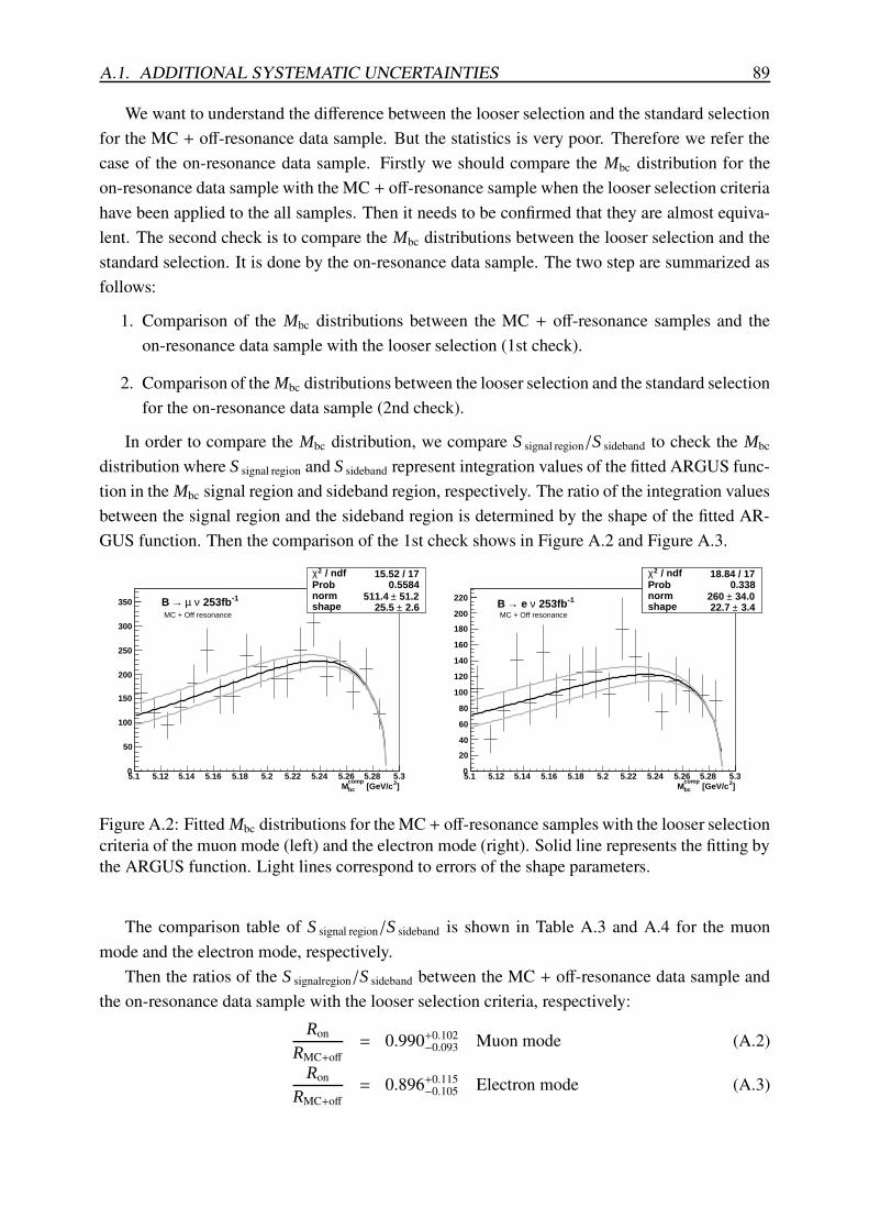
A.1. ADDITIONAL SYSTEMATIC UNCERTAINTIES 89
We want to understand the difference between the looser selection and the standard selectionfor the MC + off-resonance data sample. But the statistics is very poor. Therefore we refer thecase of the on-resonance data sample. Firstly we should compare the Mbc distribution for theon-resonance data sample with the MC + off-resonance sample when the looser selection criteriahave been applied to the all samples. Then it needs to be confirmed that they are almost equiva-lent. The second check is to compare the Mbc distributions between the looser selection and thestandard selection. It is done by the on-resonance data sample. The two step are summarized asfollows:
1. Comparison of the Mbc distributions between the MC + off-resonance samples and theon-resonance data sample with the looser selection (1st check).
2. Comparison of the Mbc distributions between the looser selection and the standard selectionfor the on-resonance data sample (2nd check).
In order to compare the Mbc distribution, we compare S signal region/S sideband to check the Mbc
distribution where S signal region and S sideband represent integration values of the fitted ARGUS func-tion in the Mbc signal region and sideband region, respectively. The ratio of the integration valuesbetween the signal region and the sideband region is determined by the shape of the fitted AR-GUS function. Then the comparison of the 1st check shows in Figure A.2 and Figure A.3.
/ ndf 2χ 15.52 / 17Prob 0.5584norm 51.2± 511.4 shape 2.6± 25.5
]2 [GeV/ccompbcM
5.1 5.12 5.14 5.16 5.18 5.2 5.22 5.24 5.26 5.28 5.30
50
100
150
200
250
300
350
/ ndf 2χ 15.52 / 17Prob 0.5584norm 51.2± 511.4 shape 2.6± 25.5
MC + Off resonance
-1 253fbν µ →B
/ ndf 2χ 18.84 / 17Prob 0.338norm 34.0± 260 shape 3.4± 22.7
]2 [GeV/ccompbcM
5.1 5.12 5.14 5.16 5.18 5.2 5.22 5.24 5.26 5.28 5.30
20
40
60
80
100
120
140
160
180
200
220
/ ndf 2χ 18.84 / 17Prob 0.338norm 34.0± 260 shape 3.4± 22.7
MC + Off resonance
-1 253fbν e →B
Figure A.2: Fitted Mbc distributions for the MC + off-resonance samples with the looser selectioncriteria of the muon mode (left) and the electron mode (right). Solid line represents the fitting bythe ARGUS function. Light lines correspond to errors of the shape parameters.
The comparison table of S signal region/S sideband is shown in Table A.3 and A.4 for the muonmode and the electron mode, respectively.
Then the ratios of the S signalregion/S sideband between the MC + off-resonance data sample andthe on-resonance data sample with the looser selection criteria, respectively:
Ron
RMC+off= 0.990+0.102
−0.093 Muon mode (A.2)
Ron
RMC+off= 0.896+0.115
−0.105 Electron mode (A.3)
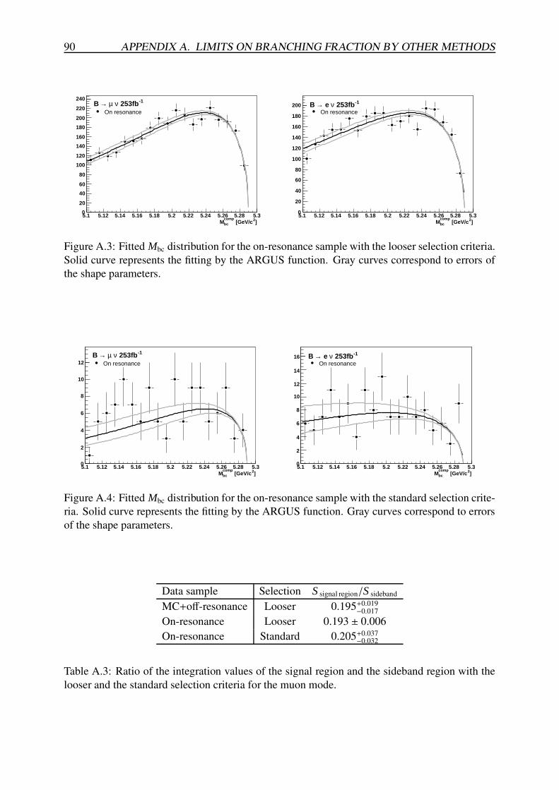
90 APPENDIX A. LIMITS ON BRANCHING FRACTION BY OTHER METHODS
]2 [GeV/ccompbcM
5.1 5.12 5.14 5.16 5.18 5.2 5.22 5.24 5.26 5.28 5.30
20
40
60
80
100
120
140
160
180
200
220
240
On resonance
-1 253fbν µ →B
]2 [GeV/ccompbcM
5.1 5.12 5.14 5.16 5.18 5.2 5.22 5.24 5.26 5.28 5.30
20
40
60
80
100
120
140
160
180
200On resonance
-1 253fbν e →B
Figure A.3: Fitted Mbc distribution for the on-resonance sample with the looser selection criteria.Solid curve represents the fitting by the ARGUS function. Gray curves correspond to errors ofthe shape parameters.
]2 [GeV/ccompbcM
5.1 5.12 5.14 5.16 5.18 5.2 5.22 5.24 5.26 5.28 5.30
2
4
6
8
10
12 On resonance
-1 253fbν µ →B
]2 [GeV/ccompbcM
5.1 5.12 5.14 5.16 5.18 5.2 5.22 5.24 5.26 5.28 5.30
2
4
6
8
10
12
14
16On resonance
-1 253fbν e →B
Figure A.4: Fitted Mbc distribution for the on-resonance sample with the standard selection crite-ria. Solid curve represents the fitting by the ARGUS function. Gray curves correspond to errorsof the shape parameters.
Data sample Selection S signal region/S sideband
MC+off-resonance Looser 0.195+0.019−0.017
On-resonance Looser 0.193 ± 0.006On-resonance Standard 0.205+0.037
−0.032
Table A.3: Ratio of the integration values of the signal region and the sideband region with thelooser and the standard selection criteria for the muon mode.
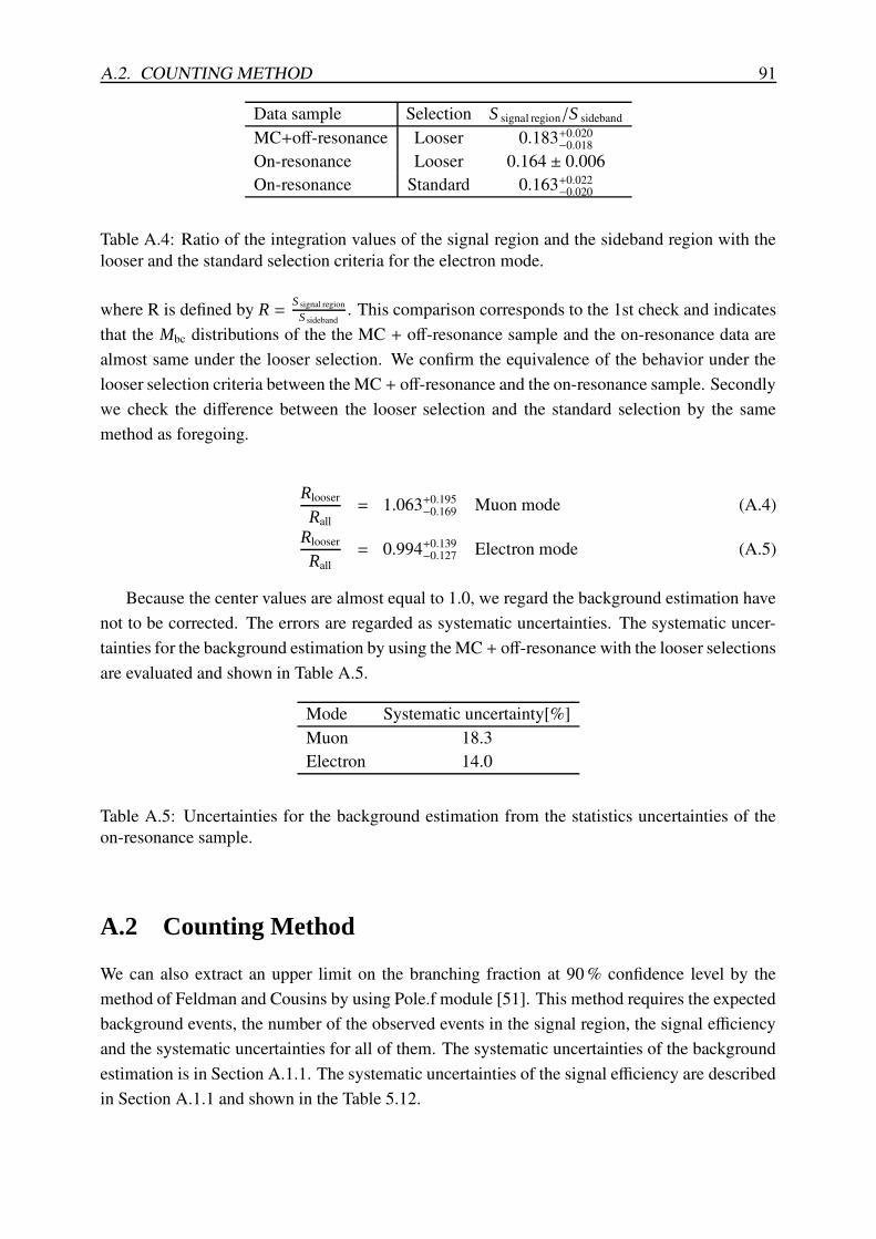
A.2. COUNTING METHOD 91
Data sample Selection S signal region/S sideband
MC+off-resonance Looser 0.183+0.020−0.018
On-resonance Looser 0.164 ± 0.006On-resonance Standard 0.163+0.022
−0.020
Table A.4: Ratio of the integration values of the signal region and the sideband region with thelooser and the standard selection criteria for the electron mode.
where R is defined by R =S signal region
S sideband. This comparison corresponds to the 1st check and indicates
that the Mbc distributions of the the MC + off-resonance sample and the on-resonance data arealmost same under the looser selection. We confirm the equivalence of the behavior under thelooser selection criteria between the MC + off-resonance and the on-resonance sample. Secondlywe check the difference between the looser selection and the standard selection by the samemethod as foregoing.
Rlooser
Rall= 1.063+0.195
−0.169 Muon mode (A.4)
Rlooser
Rall= 0.994+0.139
−0.127 Electron mode (A.5)
Because the center values are almost equal to 1.0, we regard the background estimation havenot to be corrected. The errors are regarded as systematic uncertainties. The systematic uncer-tainties for the background estimation by using the MC + off-resonance with the looser selectionsare evaluated and shown in Table A.5.
Mode Systematic uncertainty[%]Muon 18.3Electron 14.0
Table A.5: Uncertainties for the background estimation from the statistics uncertainties of theon-resonance sample.
A.2 Counting Method
We can also extract an upper limit on the branching fraction at 90 % confidence level by themethod of Feldman and Cousins by using Pole.f module [51]. This method requires the expectedbackground events, the number of the observed events in the signal region, the signal efficiencyand the systematic uncertainties for all of them. The systematic uncertainties of the backgroundestimation is in Section A.1.1. The systematic uncertainties of the signal efficiency are describedin Section A.1.1 and shown in the Table 5.12.
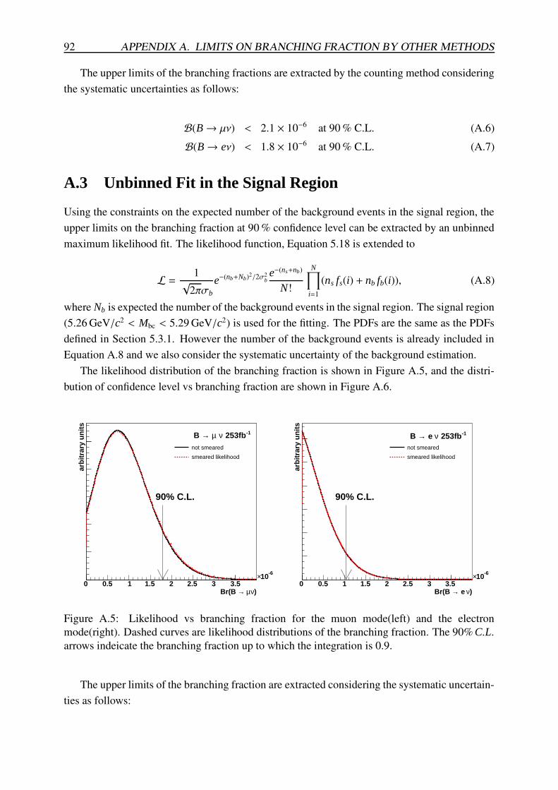
92 APPENDIX A. LIMITS ON BRANCHING FRACTION BY OTHER METHODS
The upper limits of the branching fractions are extracted by the counting method consideringthe systematic uncertainties as follows:
B(B→ µν) < 2.1 × 10⁻⁶ at 90 % C.L. (A.6)B(B→ eν) < 1.8 × 10⁻⁶ at 90 % C.L. (A.7)
A.3 Unbinned Fit in the Signal Region
Using the constraints on the expected number of the background events in the signal region, theupper limits on the branching fraction at 90 % confidence level can be extracted by an unbinnedmaximum likelihood fit. The likelihood function, Equation 5.18 is extended to
L = 1√
2πσb
e−(nb+Nb)2/2σ2be−(ns+nb)
N!
N∏
i=1(ns fs(i) + nb fb(i)), (A.8)
where Nb is expected the number of the background events in the signal region. The signal region(5.26 GeV/c2 < Mbc < 5.29 GeV/c2) is used for the fitting. The PDFs are the same as the PDFsdefined in Section 5.3.1. However the number of the background events is already included inEquation A.8 and we also consider the systematic uncertainty of the background estimation.
The likelihood distribution of the branching fraction is shown in Figure A.5, and the distri-bution of confidence level vs branching fraction are shown in Figure A.6.
)νµ →Br(B 0 0.5 1 1.5 2 2.5 3 3.5
-610×
arb
itra
ry u
nit
s
not smeared
smeared likelihood
-1 253fbν µ →B
90% C.L.
)ν e →Br(B 0 0.5 1 1.5 2 2.5 3 3.5
-610×
arb
itra
ry u
nit
s
not smeared
smeared likelihood
-1 253fbν e →B
90% C.L.
Figure A.5: Likelihood vs branching fraction for the muon mode(left) and the electronmode(right). Dashed curves are likelihood distributions of the branching fraction. The 90% C.L.arrows indeicate the branching fraction up to which the integration is 0.9.
The upper limits of the branching fraction are extracted considering the systematic uncertain-ties as follows:
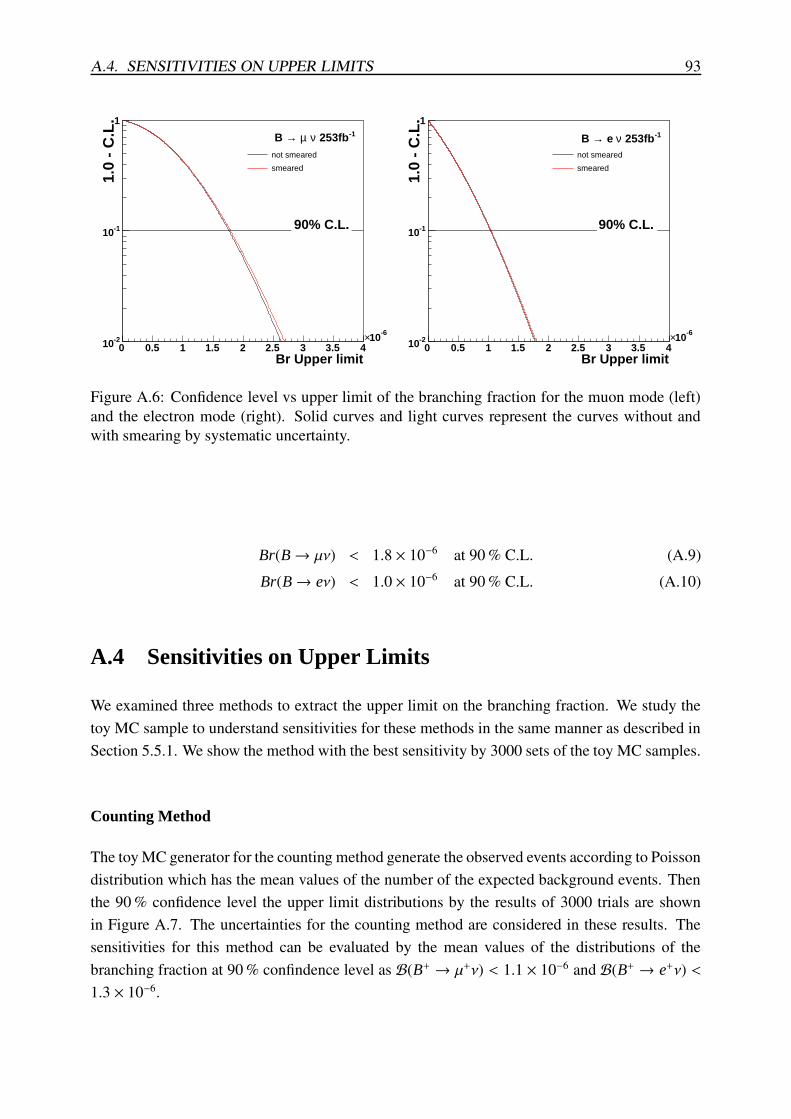
A.4. SENSITIVITIES ON UPPER LIMITS 93
Br Upper limit0 0.5 1 1.5 2 2.5 3 3.5 4
-610×
1.0
- C
.L.
-210
-110
1
not smeared
smeared
-1 253fbν µ →B
90% C.L.
Br Upper limit0 0.5 1 1.5 2 2.5 3 3.5 4
-610×
1.0
- C
.L.
-210
-110
1
not smeared
smeared
90% C.L.
-1 253fbν e →B
Figure A.6: Confidence level vs upper limit of the branching fraction for the muon mode (left)and the electron mode (right). Solid curves and light curves represent the curves without andwith smearing by systematic uncertainty.
Br(B→ µν) < 1.8 × 10⁻⁶ at 90 % C.L. (A.9)Br(B→ eν) < 1.0 × 10⁻⁶ at 90 % C.L. (A.10)
A.4 Sensitivities on Upper Limits
We examined three methods to extract the upper limit on the branching fraction. We study thetoy MC sample to understand sensitivities for these methods in the same manner as described inSection 5.5.1. We show the method with the best sensitivity by 3000 sets of the toy MC samples.
Counting Method
The toy MC generator for the counting method generate the observed events according to Poissondistribution which has the mean values of the number of the expected background events. Thenthe 90 % confidence level the upper limit distributions by the results of 3000 trials are shownin Figure A.7. The uncertainties for the counting method are considered in these results. Thesensitivities for this method can be evaluated by the mean values of the distributions of thebranching fraction at 90 % confindence level as B(B+ → µ+ν) < 1.1 × 10⁻⁶ and B(B+ → e+ν) <1.3 × 10⁻⁶.
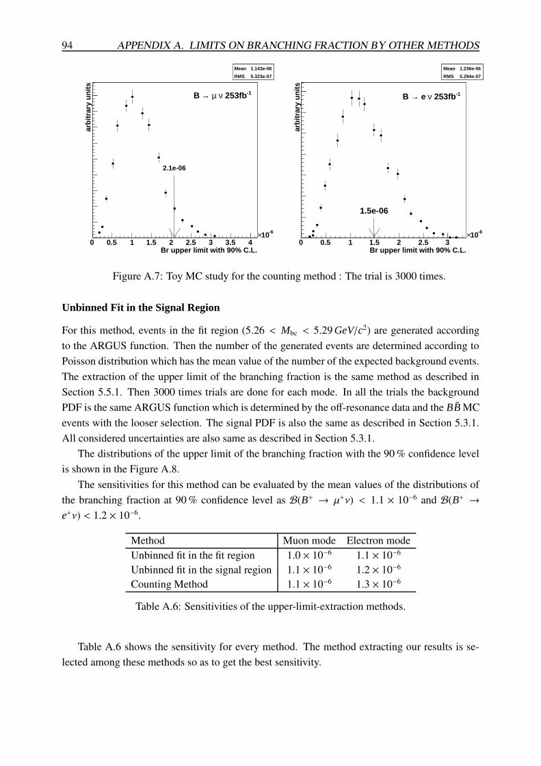
94 APPENDIX A. LIMITS ON BRANCHING FRACTION BY OTHER METHODS
Mean 1.143e-06
RMS 5.323e-07
Br upper limit with 90% C.L.0 0.5 1 1.5 2 2.5 3 3.5 4
-610×
arb
itra
ry u
nit
s
Mean 1.143e-06
RMS 5.323e-07
-1 253fbν µ →B
2.1e-06
Mean 1.236e-06
RMS 5.294e-07
Br upper limit with 90% C.L.0 0.5 1 1.5 2 2.5 3
-610×
arb
itra
ry u
nit
s
Mean 1.236e-06
RMS 5.294e-07
-1 253fbν e →B
1.5e-06
Figure A.7: Toy MC study for the counting method : The trial is 3000 times.
Unbinned Fit in the Signal Region
For this method, events in the fit region (5.26 < Mbc < 5.29 GeV/c2) are generated accordingto the ARGUS function. Then the number of the generated events are determined according toPoisson distribution which has the mean value of the number of the expected background events.The extraction of the upper limit of the branching fraction is the same method as described inSection 5.5.1. Then 3000 times trials are done for each mode. In all the trials the backgroundPDF is the same ARGUS function which is determined by the off-resonance data and the BB MCevents with the looser selection. The signal PDF is also the same as described in Section 5.3.1.All considered uncertainties are also same as described in Section 5.3.1.
The distributions of the upper limit of the branching fraction with the 90 % confidence levelis shown in the Figure A.8.
The sensitivities for this method can be evaluated by the mean values of the distributions ofthe branching fraction at 90 % confidence level as B(B+ → µ+ν) < 1.1 × 10⁻⁶ and B(B+ →e+ν) < 1.2 × 10⁻⁶.
Method Muon mode Electron modeUnbinned fit in the fit region 1.0 × 10⁻⁶ 1.1 × 10⁻⁶
Unbinned fit in the signal region 1.1 × 10⁻⁶ 1.2 × 10⁻⁶
Counting Method 1.1 × 10⁻⁶ 1.3 × 10⁻⁶
Table A.6: Sensitivities of the upper-limit-extraction methods.
Table A.6 shows the sensitivity for every method. The method extracting our results is se-lected among these methods so as to get the best sensitivity.
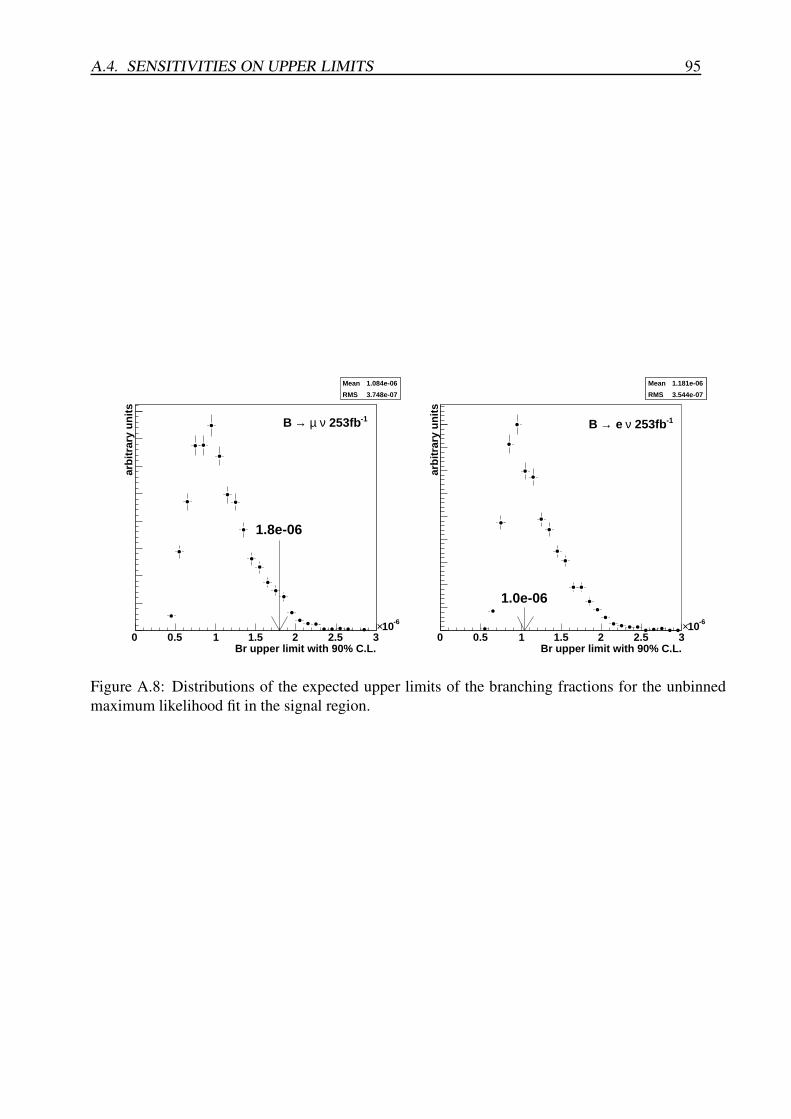
A.4. SENSITIVITIES ON UPPER LIMITS 95
Mean 1.084e-06
RMS 3.748e-07
Br upper limit with 90% C.L.0 0.5 1 1.5 2 2.5 3
-610×
arb
itra
ry u
nit
s
Mean 1.084e-06
RMS 3.748e-07
-1 253fbν µ →B
1.8e-06
Mean 1.181e-06
RMS 3.544e-07
Br upper limit with 90% C.L.0 0.5 1 1.5 2 2.5 3
-610×
arb
itra
ry u
nit
s
Mean 1.181e-06
RMS 3.544e-07
-1 253fbν e →B
1.0e-06
Figure A.8: Distributions of the expected upper limits of the branching fractions for the unbinnedmaximum likelihood fit in the signal region.

Bibliography
[1] N. Cabibbo, “Unitary Symmetry And Leptonic Decays,” Phys. Rev. Lett. 10, 531 (1963).
[2] M. Kobayashi and T. Maskawa, “CP Violation In The Renormalizeable Theory Of WeakInteraction,” Prog. Theor. Phys. 49, 652 (1973).
[3] A. B. Carter and A. I. Sanda, “CP Violation In B Meson Decays,” Phys. Rev. D 23, 1567(1981).
[4] Q. H. Kim, W. Y. Pham, “Elementary Particles and Their Interactions: Concepts and Phe-nomena,” Springer Verlag Berlin Heidelberg. (1998).
[5] L. L. Chau and W. Y. Keung, “Comments On The Parametrization Of The Kobayashi-Maskawa Matrix,” Phys. Rev. Lett. 53,1802 (1984).
[6] L. Wolfenstein, “Parameterization Of The Kobayashi-Maskawa Matrix,” Phys. Rev. Lett.51, 1945 (1983).
[7] S. Eidelman et al., [Particle Data Group], “Review of particle physics,” Phys. Lett. B 592 1(2004).
[8] M. Battaglia et al., “The CKM matrix and the unitarity triangle,” [arXiv:hep-ex/0304132].
[9] CKMfitter Group (J. Charles et al.), Eur. Phys. J. C41, 1-131 (2005) [hep-ph/0406184].
[10] A. Abashian et al., (Belle Collaboration), “Measurement of the CP violation parametersin(2φ1) in B0
d meson decays, Phys. Rev. Lett. 86, 2509 (2001) [arXiv:hep-ex/0102018].
[11] B. Aubert et al., (BaBar Collaboration), “Measurement of CP violating asymmetries in B0
decays to CP eigenstates,” Phys. Rev. Lett. 86, 2515 (2001) [arXiv:hep-ex/0102030].
[12] A. Gray et al. (HPQCD Collaboration), “The B meson decay constant from unquenchedlattice QCD,” Phys. Rev. Lett. 95, 212001 (2005). See also S. Hashimoto, “Recent resultsfrom lattice calculations,” Int. J. Mod. Phys. A 20, 5133 (2005), which quotes an averagevalue of 0.189 ± 0.027 GeV. QCD sum rules predict fB = 210 ± 19 MeV, see M. Jamin andB. O. Lange, “f(B) and f(B/s) from QCD sum rules,” Phys. Rev. D 65, 056005 (2002).
97
98 BIBLIOGRAPHY
[13] M. Neubert, “QCD Based Interpretation Of The Lepton Spectrum In Inclusive Anti-B → X(U) Lepton Anti-Neutrino Decays,” Phys. Rev. D 49, 3392 (1994) [arXiv:hep-ph/9311325].
[14] I. I. Y. Bigi et al., “On The Motion Of Heavy Quarks Inside Hadrons: Universal Distribu-tions And Inclusive Decays,” Int. J. Mod. Phys. A 9, 2467 (1994) [arXiv:hep-ph/9312311].
[15] C. W. Bauer et al., “A model independent determination of |Vub|,” Phys. Lett. B 479, 395(2000) [arXiv:hep-ph/0002161].
[16] A. Bornheim et al., (CLEO Collaboration), “Improved measurement of |Vub| with inclusivesemileptonic B decays,” Phys. Rev. Lett. 88, 231803 (2002) [arXiv:hep-ex/0202019].
[17] B. Aubert et al., (BaBar Collaboration), “Measurement of the inclusive electron spectrumin charmless semileptonic B decays near the kinematic endpoint and determination of |Vub|,”[arXiv:hep-ex/0408075].
[18] A. Limosani et al., (Belle Collaboration), “Measurement of inclusive charmless semilep-tonic B-meson decays at the endpoint of the electron momentum spectrum,” Phys. Lett. B621, 28 (2005) [arXiv:hep-ex/0504046].
[19] I. Bizjak et al., (Belle Collaboration), “Measurement of the inclusive charmless semilep-tonic partial branching fraction of B mesons and determination of |Vub| using the full recon-struction tag,” Phys. Rev. Lett. 95, 241801 (2005) [arXiv:/hep-ex/0504046]; B. Aubert et
al., (BaBar Collaboration), “Measurement of the inclusive charmless semileptonic branch-ing ratio of B mesons and determination of |Vub|,” Phys. Rev. Lett. 92, 071802 (2004)[arXiv:hep-ex/0307062].
[20] M. Okamoto et al., “Semileptonic D → π/K and B → πD decays in 2+1 flavor latticeQCD,” Nucl. Phys. Proc. Suppl. 140, 461 (2005) [arXiv:hep-lat/0409116].
[21] J. Shigemitsu et al., ‘Semileptonic B decays with N( f ) = 2 + 1 dynamical quarks,” Nucl.Phys. Proc. Suppl. 140, 464 (2005) [arXiv:hep-lat/0408019].
[22] P. Ball and R. Zwicky, ‘Semileptonic B decays with N(f) = 2+1 dynamical quarks,” Phys.Rev. D 71, 014015 (2005) [arXiv:hep-ph/0406232].
[23] R. Kowalewski and T. Mannel, “Determination of Vcb and Vub,” in W. M. Yao et al. [ParticleData Group], J. Phys. G 33, 867 (2006).
[24] M. Battaglia and L. Gibbons, “Determination of |Vub|,” in S. Eidelman et al., [Particle DataGroup], Phys. Lett. B 592, 793 (2004).
[25] K. Ikado et al. (Belle Collaboration), “Evidence of the purely leptonic decay B− → τ−ντ,”Phys. Rev. Lett. 97, 251802 (2006).
BIBLIOGRAPHY 99
[26] B. Aubert et al. (BaBar Collaboration), “Search for the rare leptonic decay B+ → µ+νµ,”Phys. Rev. Lett. 92, 221803 (2004).
[27] M. Artuso el al. (CLEO Collaboration), “A Search for B → lepton anti-lepton-neutrino,”Phys. Rev. Lett. 75, 785 (1995).
[28] K. Abe et al. (Belle Collaboration), “Search for B+ → µ+ν and B+ → `+νγ decays,” hep-ex/0408132 (2004).
[29] B. Aubert et al. (BaBar Collaboration), “A search for the decays B+ → e+νe and B+ → µ+νµ
using hadronic-tag reconstruction,” hep-ex/0607110 (2006).
[30] W. S. Hou, “Enhanced charged Higgs boson effects in B− → τντ, µ−νµ and B→ τνtau+X,”Phys. Rev. D 48, 2342 (1993).
[31] S. Kurokawa and E. Kikutani, “Overview of the KEKB accelerators,” Nucl. Instrum. Meth.A 499, 1 (2003).
[32] A. Abashian et al., (Belle Collaboration), “The Belle detector,” Nucl. Instrum. Meth. A479, 117 (2002).
[33] H. Aihara, “The Belle silicon vertex detector,” Nucl. Instrum. Meth. A 466, 268 (2001).[arXiv:hep-ex/0011028].
[34] H. Hirano el at., “A high resolution cylindrical drift chamber for the KEK B-factory,” Nucl.Instrum. Meth. A 455, 294 (2000).
[35] T. Sumiyoshi et al., “Silica aerogel Cherenkov counter for the KEK B-factory experiment,”Nucl. Instrum. Meth. A 433, 385 (1999).
[36] T. Iijima et al., “Aerogel Cherenkov counter for the BELLE detector,” Nucl. Instrum. Meth.A 453, 321 (2000).
[37] H. Kichimi et al., “The BELLE TOF system,” Nucl. Instrum. Meth. A 453, 321 (2000).
[38] A. Abashian et al., (Belle Collaboration) “The K(L)/mu detector subsystem for the BELLEexperiment at the KEKB factory,” Nucl. Instrum. Meth. A 449, 112 (2000).
[39] The CLEO QQ generator, see http://www.lns.cornell.edu/public/CLEO/soft/QQ/.
[40] D. J. Lange, “The EvtGen particle decay simulation package,” Nucl. Instrum. Meth. A 462,152 (2001).
[41] T. Sjostrand, “PYTHIA 5.7 and JETSET 7.4: Physics and manual,” arXiv:hep-ph/9508391.
[42] T. Sjostrand, P. Eden, C. Friberg, L. Lonnblad, G. Miu, S. Mrenna and E. Norrbin, “High-energy-physics event generation with PYTHIA 6.1,” Computer Physics Commun. 135 238(2001).

100 BIBLIOGRAPHY
[43] B. Andersson, G. Gustafson, G. Ingelman and T. Sjostrand, “Parton Fragmentation AndString Dynamics,” Phys. Repot. 97, 31 (1983).
[44] R. Brun, R. Hagelberg, M. Hanstroul, and J. C. Lasalle, “Geant: Simulation Program ForParticle Physics Experiments. User Guide And Reference Manual,” CERN-DD-78-2-REV; R. Brun et al., GEANT 3.21, CERN Report DD/EE/84-1 (1984).
[45] Tracking Group (Belle Collaboration), “Charged Particle Tracking in Belle,” Belle Note327 (2000).
[46] A. Abashian et al., (Belle Collaboration) “Muon identification in the Belle experiment atKEKB,” Nucl. Instrum. Meth. A 491, 69 (2002).
[47] K. Hanagaki, H. Kakuno, H. Ikeda, T. Iijima and T. Tsukamoto, “Electron identification inBelle,” Nucl. Instrum. Meth. A485, 490 (2002) arXiv:hep-ex/0108044.
[48] H. Kakuno, “Measurement of |Vub| through Charmless Semileptonic B-meson Decay,”Tokyo Institute of Technology, Doctor Thesis (2003).
[49] G. C. Fox and S. Wolfram, “Observables For The Analysis Of Event Shapes In e+e− Anni-hilation And Other Processes,” Phys. Rev. Lett. 41, 1581 (1978).
[50] K. Abe et al., (Belle Collaboration), “A measurement of the branching fraction for theinclusive B→ Xsγ decays with Belle,” Phys. Lett. B 511, 151 (2001).
[51] J.Conrad et al., “Including systematic uncertainties in confidence interval construction forPoisson statistics,” Phys. Rev. D 67, 012002 (2003).