A Review of SolutionTechniques for Unsteady

Incompressible Flow

David SilvesterSchool of Mathematics

University of Manchester

Zeist 2009 – p. 1/57

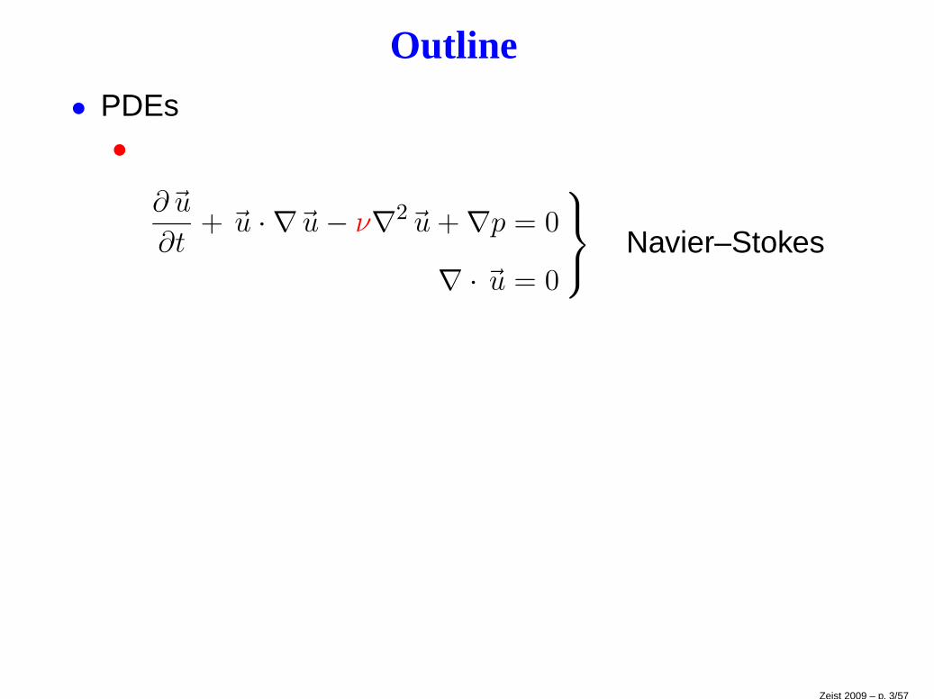
Outline

• PDEs

• Review : 1966 – 1999

• Update : 2000 – 2009

Zeist 2009 – p. 2/57

Outline

• PDEs•

∂~u

∂t+ ~u · ∇~u− ν∇2~u+ ∇p = 0

∇ · ~u = 0

Navier–Stokes

Zeist 2009 – p. 3/57

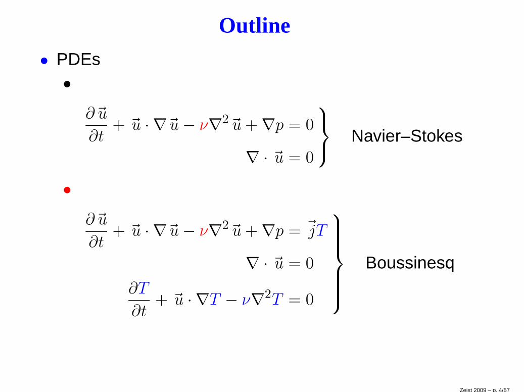
Outline

• PDEs•

∂~u

∂t+ ~u · ∇~u− ν∇2~u+ ∇p = 0

∇ · ~u = 0

Navier–Stokes

•∂~u

∂t+ ~u · ∇~u− ν∇2~u+ ∇p = ~jT

∇ · ~u = 0

∂T

∂t+ ~u · ∇T − ν∇2T = 0

Boussinesq

Zeist 2009 – p. 4/57

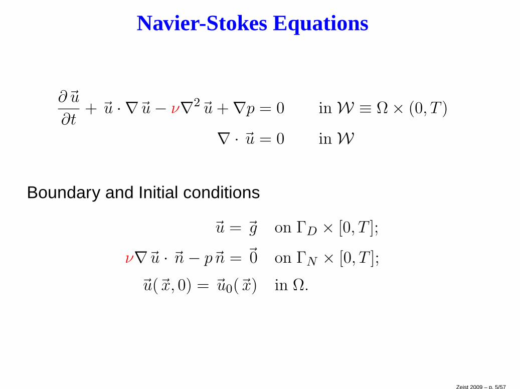
Navier-Stokes Equations

∂~u

∂t+ ~u · ∇~u− ν∇2~u+ ∇p = 0 in W ≡ Ω × (0, T )

∇ · ~u = 0 in W

Boundary and Initial conditions

~u = ~g on ΓD × [0, T ];

ν∇~u · ~n− p~n = ~0 on ΓN × [0, T ];

~u(~x, 0) = ~u0(~x) in Ω.

Zeist 2009 – p. 5/57

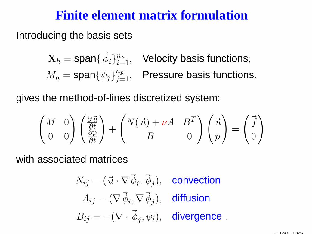
Finite element matrix formulation

Introducing the basis sets

Xh = span~φinu

i=1, Velocity basis functions;

Mh = spanψjnp

j=1, Pressure basis functions.

gives the method-of-lines discretized system:(

M 0

0 0

)(∂~u∂t∂p∂t

)

+

(

N(~u) + νA BT

B 0

)(

~u

p

)

=

(~f

0

)

with associated matrices

Nij = (~u · ∇~φi, ~φj), convection

Aij = (∇~φi,∇~φj), diffusion

Bij = −(∇ · ~φj , ψi), divergence .Zeist 2009 – p. 6/57

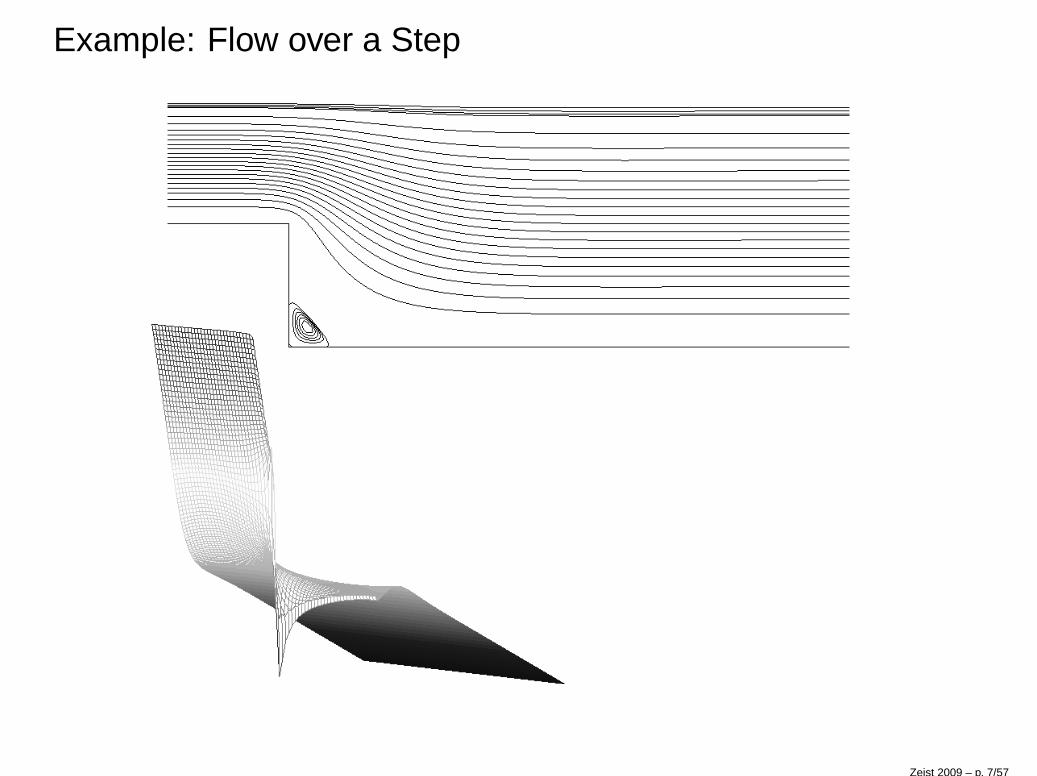
Example: Flow over a Step

Zeist 2009 – p. 7/57

Outline

• PDEs

• Review : 1966 – 1999

• Update : 2000 – 2009

Zeist 2009 – p. 8/57

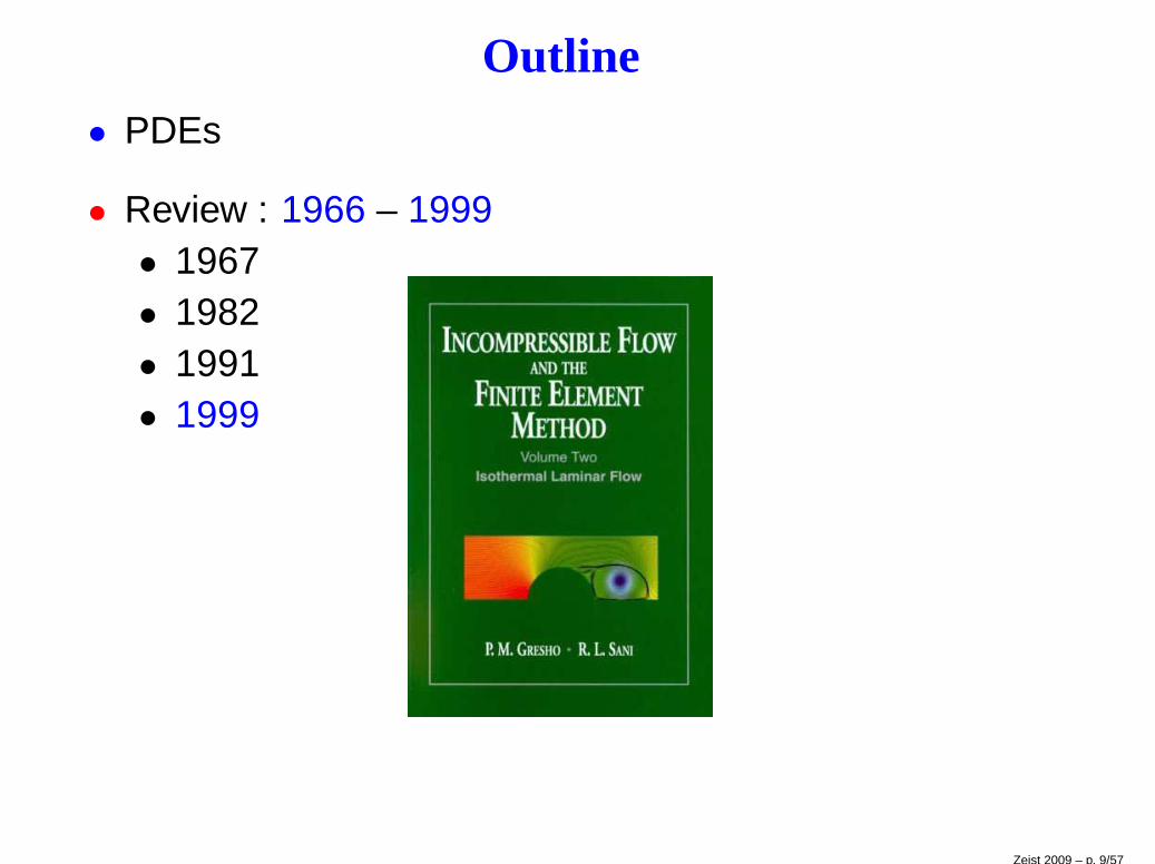
Outline

• PDEs

• Review : 1966 – 1999• 1967• 1982• 1991• 1999

Zeist 2009 – p. 9/57

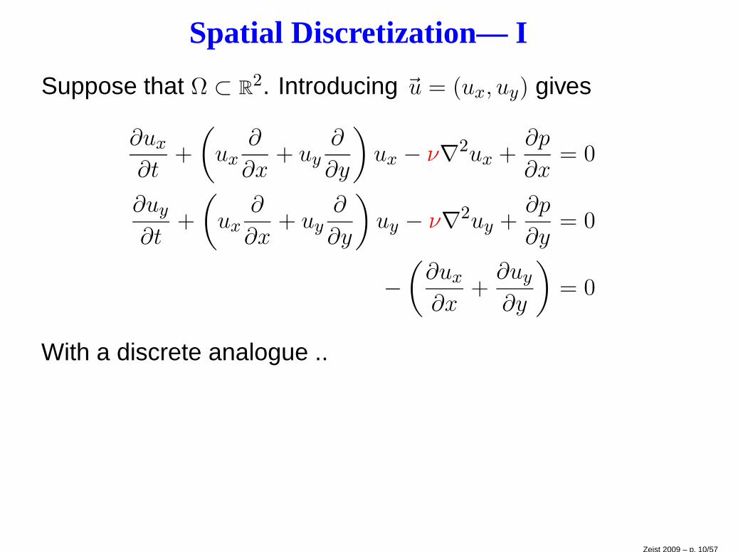
Spatial Discretization— I

Suppose that Ω ⊂ R2. Introducing ~u = (ux, uy) gives

∂ux

∂t+

(

ux∂

∂x+ uy

∂

∂y

)

ux − ν∇2ux +∂p

∂x= 0

∂uy

∂t+

(

ux∂

∂x+ uy

∂

∂y

)

uy − ν∇2uy +∂p

∂y= 0

−(∂ux

∂x+∂uy

∂y

)

= 0

With a discrete analogue ..

Zeist 2009 – p. 10/57

Spatial Discretization— I

Suppose that Ω ⊂ R2. Introducing ~u = (ux, uy) gives

∂ux

∂t+

(

ux∂

∂x+ uy

∂

∂y

)

ux − ν∇2ux +∂p

∂x= 0

∂uy

∂t+

(

ux∂

∂x+ uy

∂

∂y

)

uy − ν∇2uy +∂p

∂y= 0

−(∂ux

∂x+∂uy

∂y

)

= 0

With a discrete analogue ..

M 0 0

0 M 0

0 0 0

∂αx

∂t∂αy

∂t∂αp

∂t

+

F 0 BTx

0 F BTy

Bx By 0

αx

αy

αp

=

0

0

0

Zeist 2009 – p. 10/57

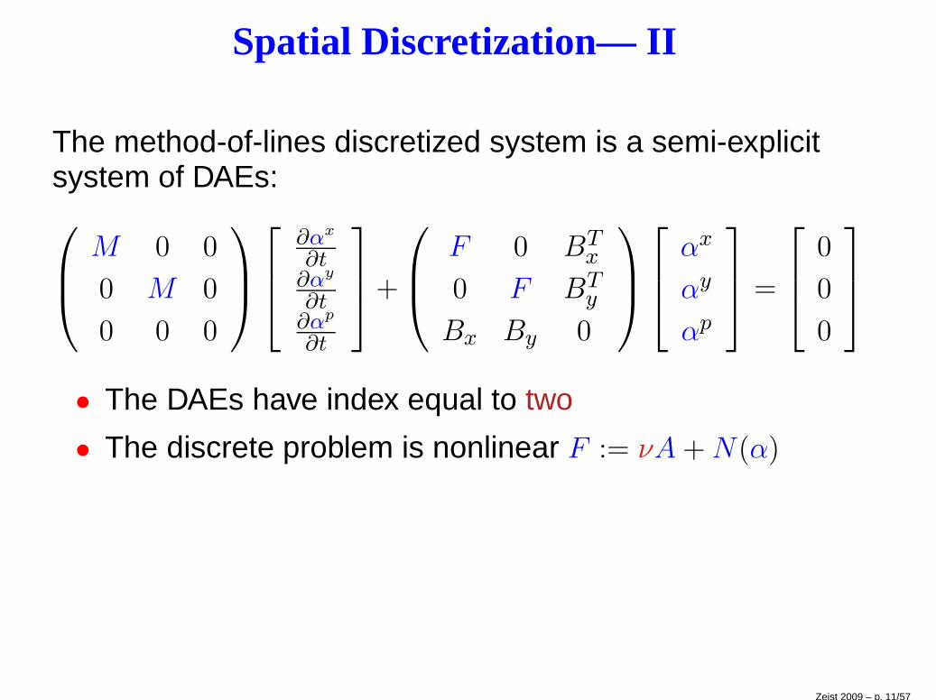
Spatial Discretization— II

The method-of-lines discretized system is a semi-explicitsystem of DAEs:

M 0 0

0 M 0

0 0 0

∂αx

∂t∂αy

∂t∂αp

∂t

+

F 0 BTx

0 F BTy

Bx By 0

αx

αy

αp

=

0

0

0

• The DAEs have index equal to two

• The discrete problem is nonlinear F := νA+N(α)

Zeist 2009 – p. 11/57

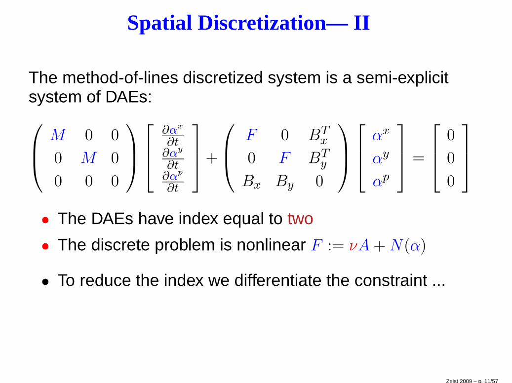
Spatial Discretization— II

The method-of-lines discretized system is a semi-explicitsystem of DAEs:

M 0 0

0 M 0

0 0 0

∂αx

∂t∂αy

∂t∂αp

∂t

+

F 0 BTx

0 F BTy

Bx By 0

αx

αy

αp

=

0

0

0

• The DAEs have index equal to two

• The discrete problem is nonlinear F := νA+N(α)

• To reduce the index we differentiate the constraint ...

Zeist 2009 – p. 11/57

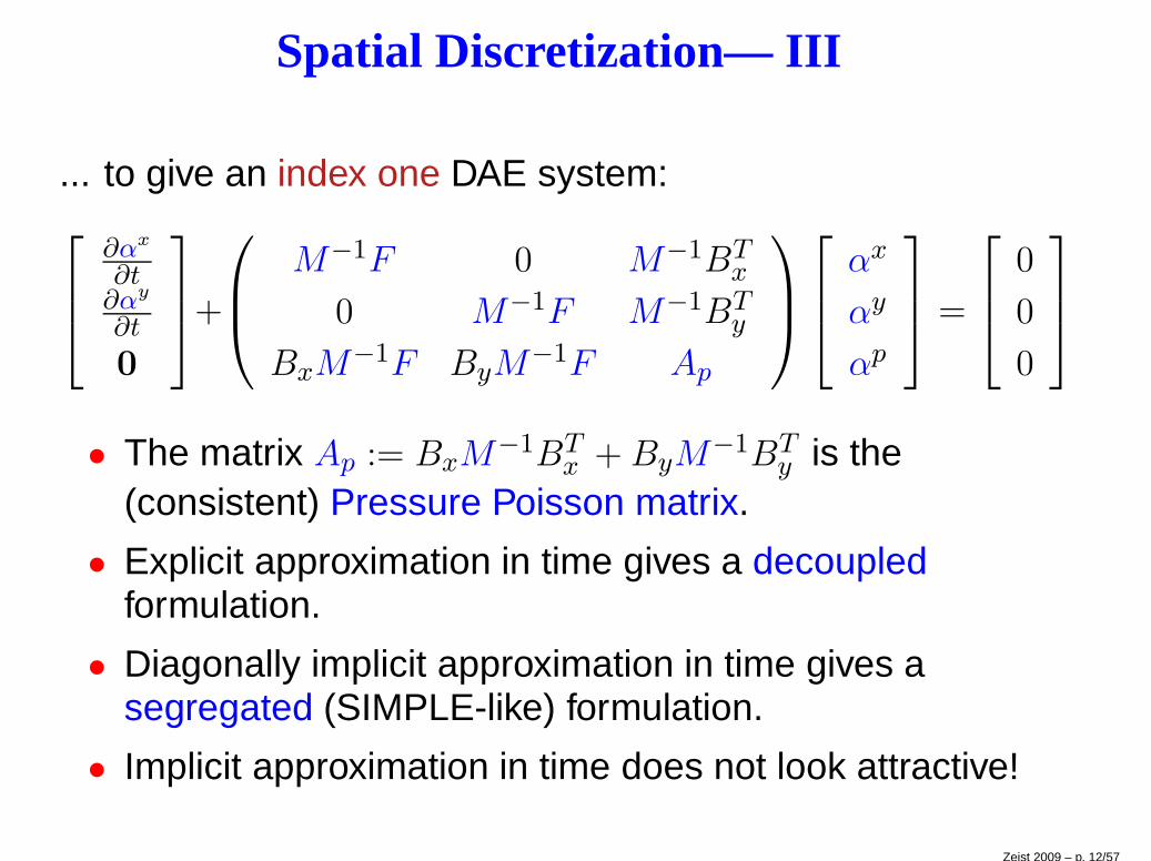
Spatial Discretization— III

... to give an index one DAE system:

∂αx

∂t∂αy

∂t

0

+

M−1F 0 M−1BTx

0 M−1F M−1BTy

BxM−1F ByM

−1F Ap

αx

αy

αp

=

0

0

0

• The matrix Ap := BxM−1BT

x + ByM−1BT

y is the(consistent) Pressure Poisson matrix.

• Explicit approximation in time gives a decoupledformulation.

• Diagonally implicit approximation in time gives asegregated (SIMPLE-like) formulation.

• Implicit approximation in time does not look attractive!

Zeist 2009 – p. 12/57

(

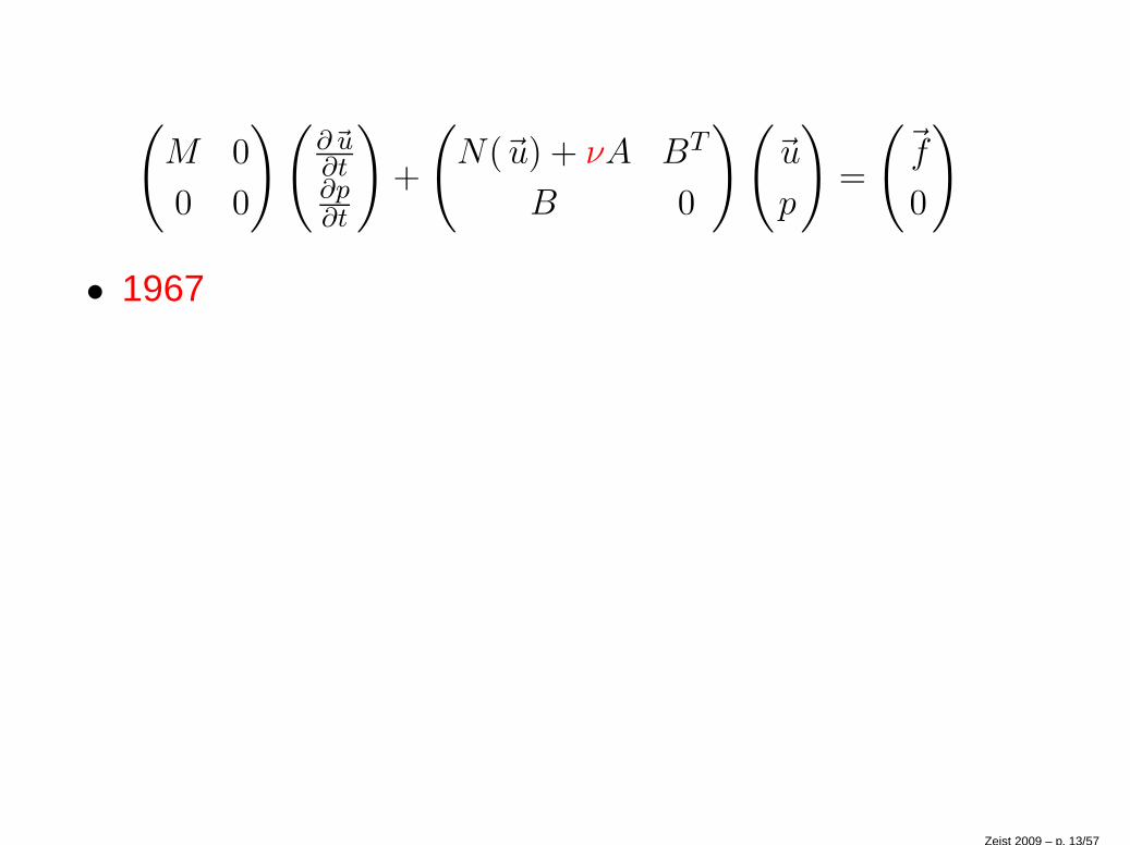
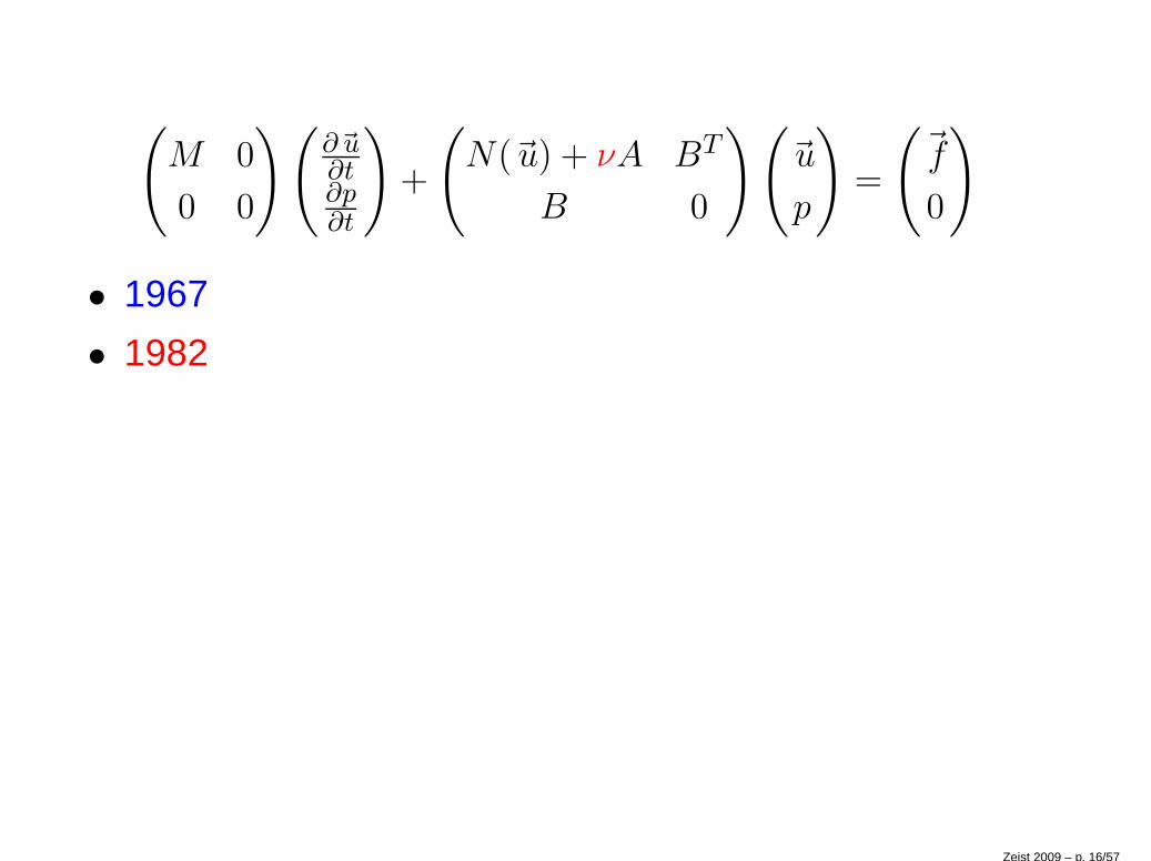
M 0

0 0

)(∂~u∂t∂p∂t

)

+

(

N(~u) + νA BT

B 0

)(

~u

p

)

=

(~f

0

)

• 1967

Zeist 2009 – p. 13/57

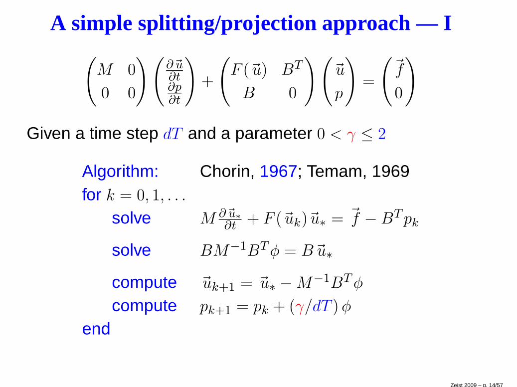
A simple splitting/projection approach — I(

M 0

0 0

)(∂~u∂t∂p∂t

)

+

(

F (~u) BT

B 0

)(

~u

p

)

=

(~f

0

)

Given a time step dT and a parameter 0 < γ ≤ 2

Algorithm: Chorin, 1967; Temam, 1969for k = 0, 1, . . .

solve M ∂~u∗

∂t + F (~uk)~u∗ = ~f − BTpk

solve BM−1BTφ = B~u∗

compute ~uk+1 = ~u∗ −M−1BTφ

compute pk+1 = pk + (γ/dT )φ

end

Zeist 2009 – p. 14/57

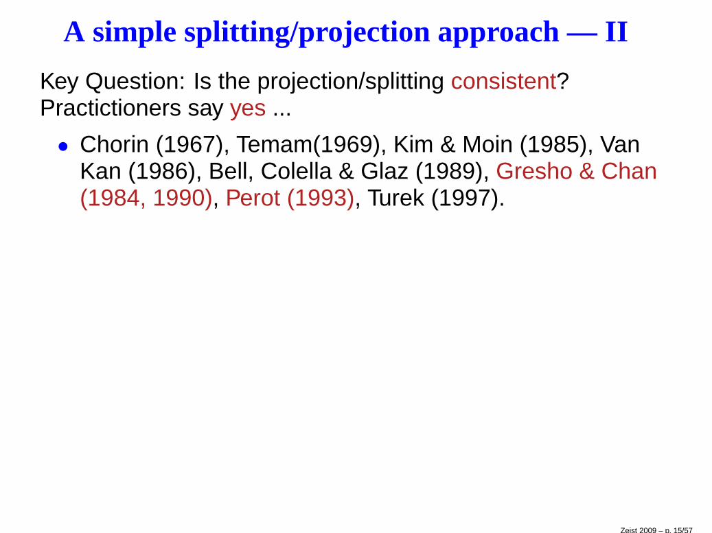
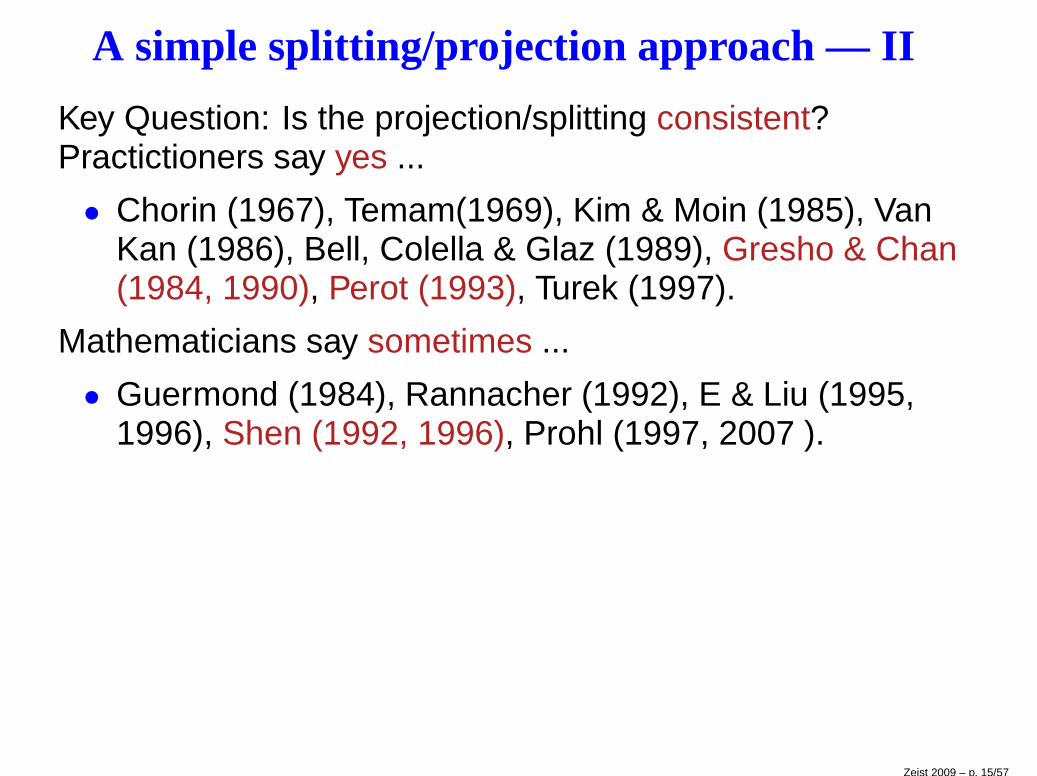
A simple splitting/projection approach — II

Key Question: Is the projection/splitting consistent?

Zeist 2009 – p. 15/57

A simple splitting/projection approach — II

Key Question: Is the projection/splitting consistent?Practictioners say yes ...

• Chorin (1967), Temam(1969), Kim & Moin (1985), VanKan (1986), Bell, Colella & Glaz (1989), Gresho & Chan(1984, 1990), Perot (1993), Turek (1997).

Zeist 2009 – p. 15/57

A simple splitting/projection approach — II

Key Question: Is the projection/splitting consistent?Practictioners say yes ...

• Chorin (1967), Temam(1969), Kim & Moin (1985), VanKan (1986), Bell, Colella & Glaz (1989), Gresho & Chan(1984, 1990), Perot (1993), Turek (1997).

Mathematicians say sometimes ...

• Guermond (1984), Rannacher (1992), E & Liu (1995,1996), Shen (1992, 1996), Prohl (1997, 2007 ).

Zeist 2009 – p. 15/57

(

M 0

0 0

)(∂~u∂t∂p∂t

)

+

(

N(~u) + νA BT

B 0

)(

~u

p

)

=

(~f

0

)

• 1967

• 1982

Zeist 2009 – p. 16/57

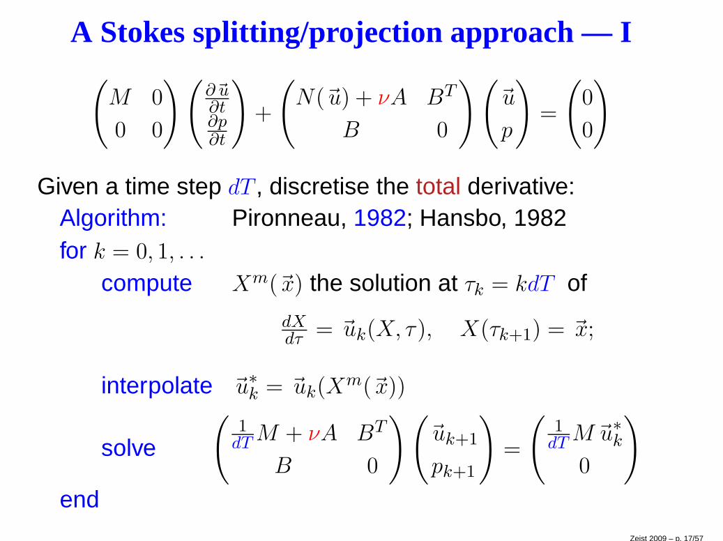
A Stokes splitting/projection approach — I(

M 0

0 0

)(∂~u∂t∂p∂t

)

+

(

N(~u) + νA BT

B 0

)(

~u

p

)

=

(

0

0

)

Given a time step dT , discretise the total derivative:Algorithm: Pironneau, 1982; Hansbo, 1982for k = 0, 1, . . .

compute Xm(~x) the solution at τk = kdT of

dXdτ = ~uk(X, τ), X(τk+1) = ~x;

interpolate ~u∗k = ~uk(Xm(~x))

solve

(1

dTM + νA BT

B 0

)(

~uk+1

pk+1

)

=

(1

dTM~u∗k0

)

endZeist 2009 – p. 17/57

A simple splitting/projection approach — II

Key1 Question: Is the total derivative approximation stablenumerically ?

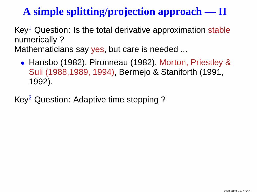
Zeist 2009 – p. 18/57

A simple splitting/projection approach — II

Key1 Question: Is the total derivative approximation stablenumerically ?Mathematicians say yes, but care is needed ...

• Hansbo (1982), Pironneau (1982), Morton, Priestley &Suli (1988,1989, 1994), Bermejo & Staniforth (1991,1992).

Zeist 2009 – p. 18/57

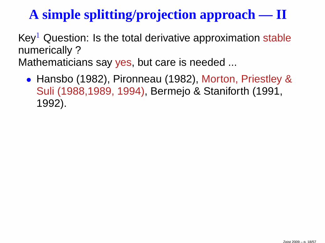
A simple splitting/projection approach — II

Key1 Question: Is the total derivative approximation stablenumerically ?Mathematicians say yes, but care is needed ...

• Hansbo (1982), Pironneau (1982), Morton, Priestley &Suli (1988,1989, 1994), Bermejo & Staniforth (1991,1992).

Key2 Question: Adaptive time stepping ?

Zeist 2009 – p. 18/57

(

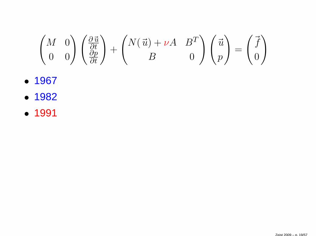
M 0

0 0

)(∂~u∂t∂p∂t

)

+

(

N(~u) + νA BT

B 0

)(

~u

p

)

=

(~f

0

)

• 1967

• 1982

• 1991

Zeist 2009 – p. 19/57

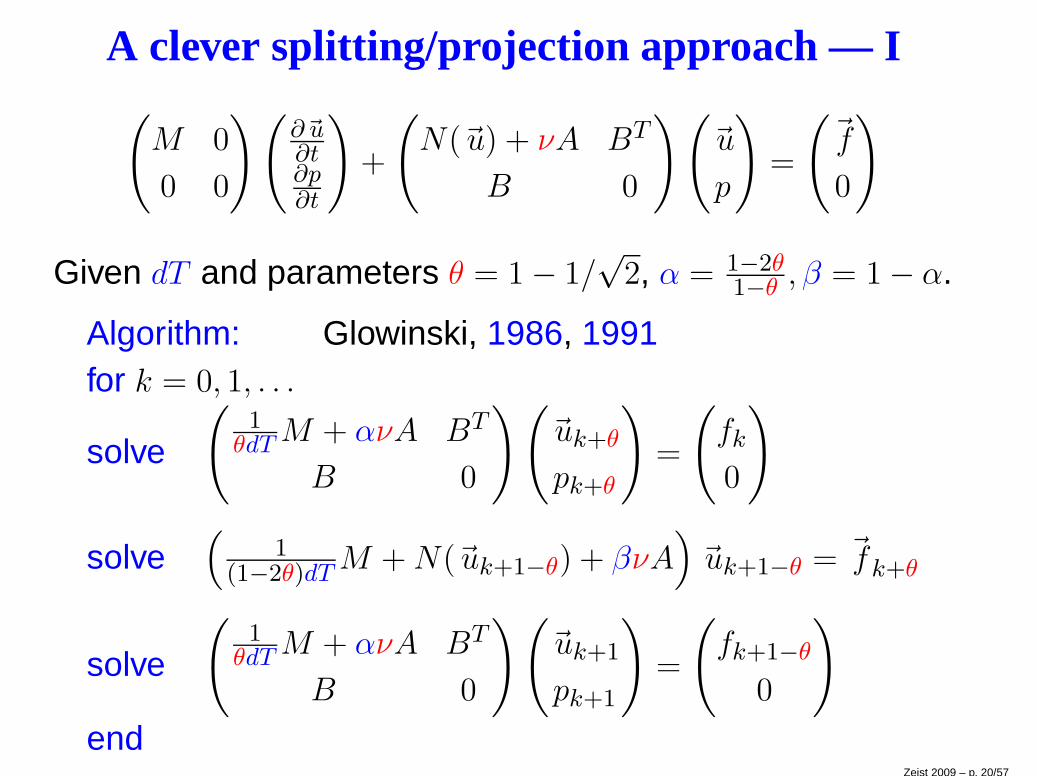
A clever splitting/projection approach — I(

M 0

0 0

)(∂~u∂t∂p∂t

)

+

(

N(~u) + νA BT

B 0

)(

~u

p

)

=

(~f

0

)

Given dT and parameters θ = 1 − 1/√

2, α = 1−2θ1−θ , β = 1 − α.

Algorithm: Glowinski, 1986, 1991for k = 0, 1, . . .

solve

(1

θdTM + ανA BT

B 0

)(

~uk+θ

pk+θ

)

=

(

fk

0

)

solve(

1(1−2θ)dTM +N(~uk+1−θ) + βνA

)

~uk+1−θ = ~fk+θ

solve

(1

θdTM + ανA BT

B 0

)(

~uk+1

pk+1

)

=

(

fk+1−θ

0

)

endZeist 2009 – p. 20/57

A clever splitting/projection approach — II

Key1 Question: Is the algorithm over-complicated?

Zeist 2009 – p. 21/57

A clever splitting/projection approach — II

Key1 Question: Is the algorithm over-complicated?Mathematicians say no, ...

• Glowinski & Dean (1984, 1993) , Bristeau et al. (1985),Rannacher (1989, 1990), Turek (1996), Smith &Silvester (1997).

Zeist 2009 – p. 21/57

A clever splitting/projection approach — II

Key1 Question: Is the algorithm over-complicated?Mathematicians say no, ...

• Glowinski & Dean (1984, 1993) , Bristeau et al. (1985),Rannacher (1989, 1990), Turek (1996), Smith &Silvester (1997).

Key2 Question: Adaptive time stepping ?

Zeist 2009 – p. 21/57

• Update : 2000 – 2009

Philip Gresho & David Griffiths & David SilvesterAdaptive time-stepping for incompressible flow; part I:scalar advection-diffusion, SIAM J. ScientificComputing, 30: 2018–2054, 2008.

David Kay & Philip Gresho & David Griffiths & DavidSilvester Adaptive time-stepping for incompressibleflow; part II: Navier-Stokes equations. MIMS Eprint2008.61.

Zeist 2009 – p. 22/57

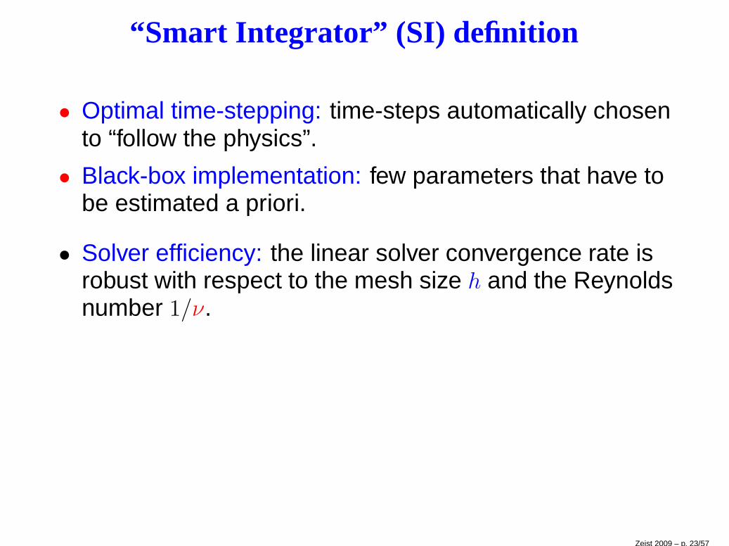
“Smart Integrator” (SI) definition

• Optimal time-stepping: time-steps automatically chosento “follow the physics”.

• Black-box implementation: few parameters that have tobe estimated a priori.

Zeist 2009 – p. 23/57

“Smart Integrator” (SI) definition

• Optimal time-stepping: time-steps automatically chosento “follow the physics”.

• Black-box implementation: few parameters that have tobe estimated a priori.

• Solver efficiency: the linear solver convergence rate isrobust with respect to the mesh size h and the Reynoldsnumber 1/ν.

Zeist 2009 – p. 23/57

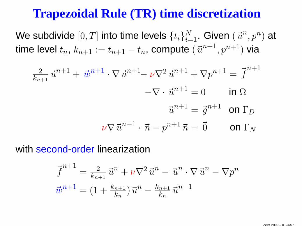
Trapezoidal Rule (TR) time discretization

We subdivide [0, T ] into time levels tiNi=1. Given (~un, pn) at

time level tn, kn+1 := tn+1 − tn, compute (~un+1, pn+1) via

2kn+1

~un+1 + ~wn+1 · ∇~un+1− ν∇2~un+1 + ∇pn+1 = ~fn+1

−∇ · ~un+1 = 0 in Ω

~un+1 = ~gn+1 on ΓD

ν∇~un+1 · ~n− pn+1~n = ~0 on ΓN

with second-order linearization

~fn+1

= 2kn+1

~un + ν∇2~un − ~un · ∇~un −∇pn

~wn+1 = (1 + kn+1

kn)~un − kn+1

kn~un−1

Zeist 2009 – p. 24/57

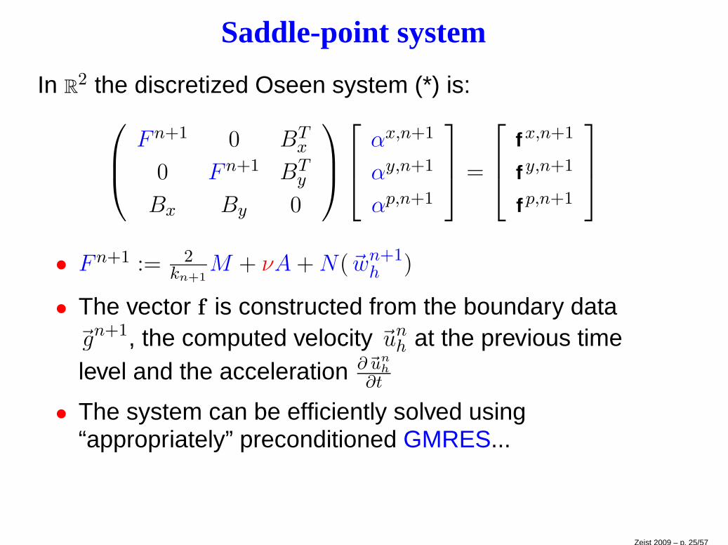
Saddle-point system

In R2 the discretized Oseen system (*) is:

Fn+1 0 BTx

0 Fn+1 BTy

Bx By 0

αx,n+1

αy,n+1

αp,n+1

=

f x,n+1

f y,n+1

f p,n+1

• Fn+1 := 2kn+1

M + νA+N(~wn+1h )

• The vector f is constructed from the boundary data~gn+1, the computed velocity ~un

h at the previous timelevel and the acceleration ∂~un

h

∂t

• The system can be efficiently solved using“appropriately” preconditioned GMRES...

Zeist 2009 – p. 25/57

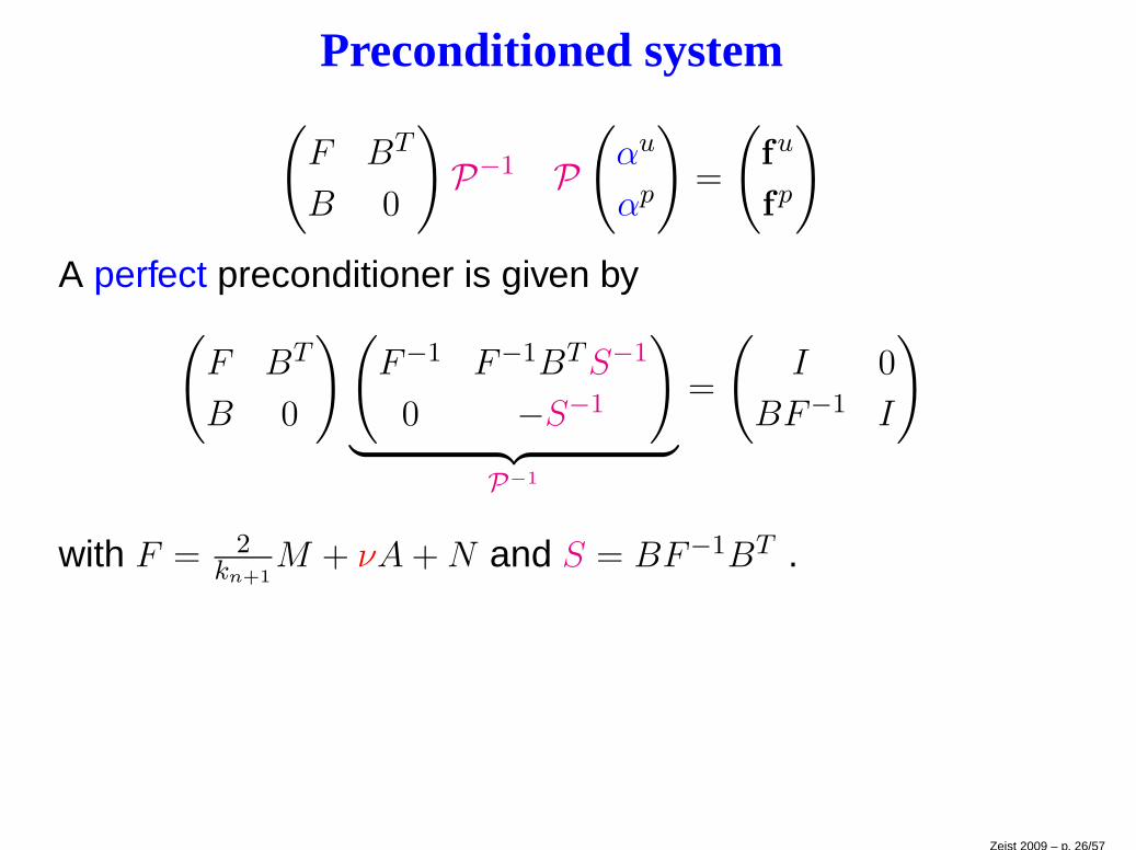
Preconditioned system(

F BT

B 0

)

P−1 P(

αu

αp

)

=

(

fu

fp

)

A perfect preconditioner is given by(

F BT

B 0

)(

F−1 F−1BTS−1

0 −S−1

)

︸ ︷︷ ︸

P−1

=

(

I 0

BF−1 I

)

with F = 2kn+1

M + νA+N and S = BF−1BT .

Zeist 2009 – p. 26/57

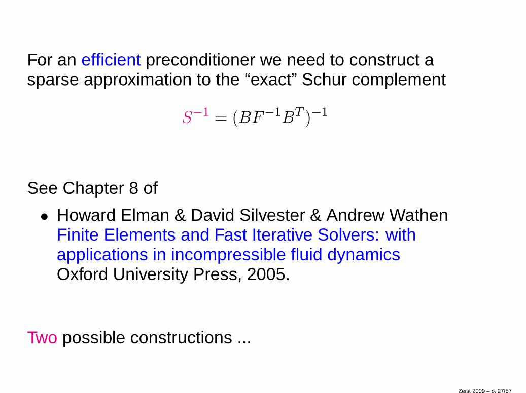
For an efficient preconditioner we need to construct asparse approximation to the “exact” Schur complement

S−1 = (BF−1BT )−1

See Chapter 8 of

• Howard Elman & David Silvester & Andrew WathenFinite Elements and Fast Iterative Solvers: withapplications in incompressible fluid dynamicsOxford University Press, 2005.

Two possible constructions ...

Zeist 2009 – p. 27/57

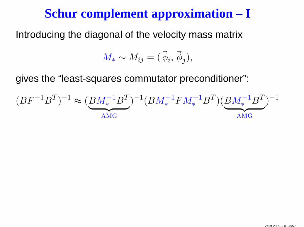
Schur complement approximation – I

Introducing the diagonal of the velocity mass matrix

M∗ ∼Mij = (~φi, ~φj),

gives the “least-squares commutator preconditioner”:

(BF−1BT )−1 ≈ (BM−1∗ BT

︸ ︷︷ ︸

amg

)−1(BM−1∗ FM−1

∗ BT )(BM−1∗ BT

︸ ︷︷ ︸

amg

)−1

Zeist 2009 – p. 28/57

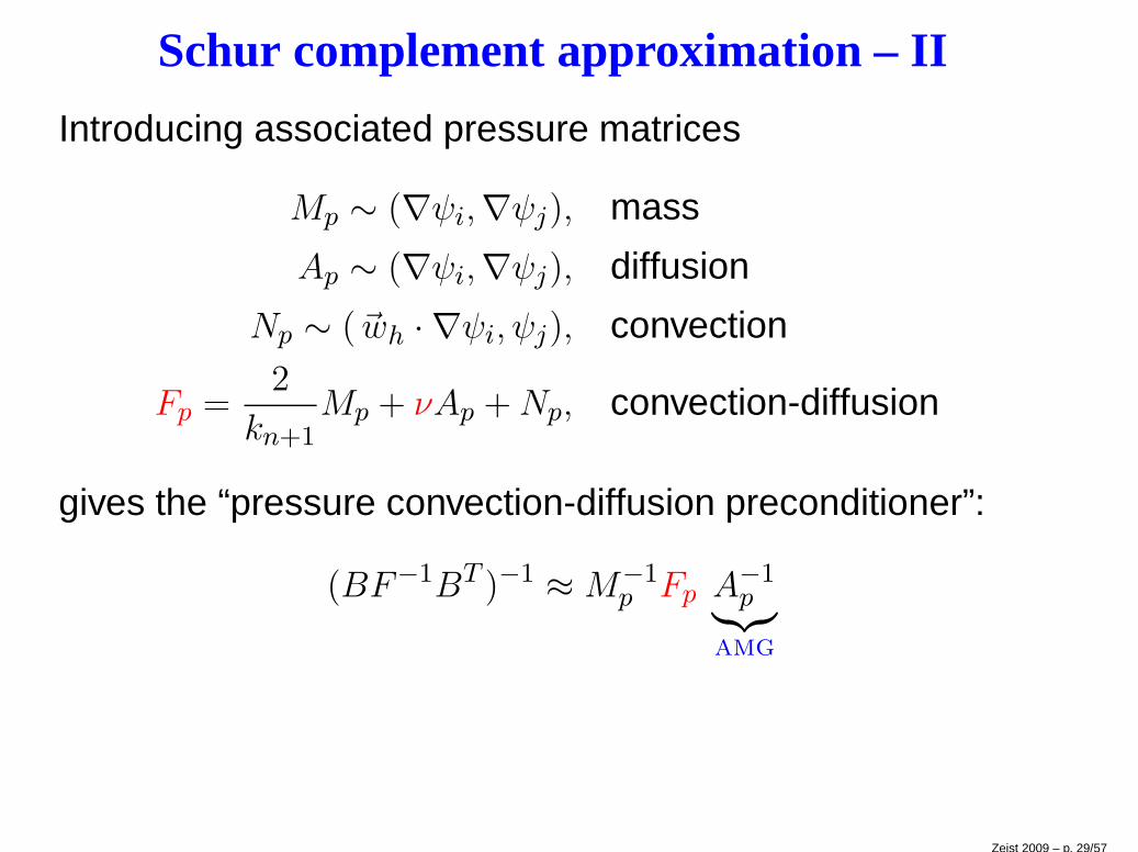
Schur complement approximation – II

Introducing associated pressure matrices

Mp ∼ (∇ψi,∇ψj), mass

Ap ∼ (∇ψi,∇ψj), diffusion

Np ∼ (~wh · ∇ψi, ψj), convection

Fp =2

kn+1Mp + νAp +Np, convection-diffusion

gives the “pressure convection-diffusion preconditioner”:

(BF−1BT )−1 ≈M−1p Fp A

−1p︸︷︷︸

amg

Zeist 2009 – p. 29/57

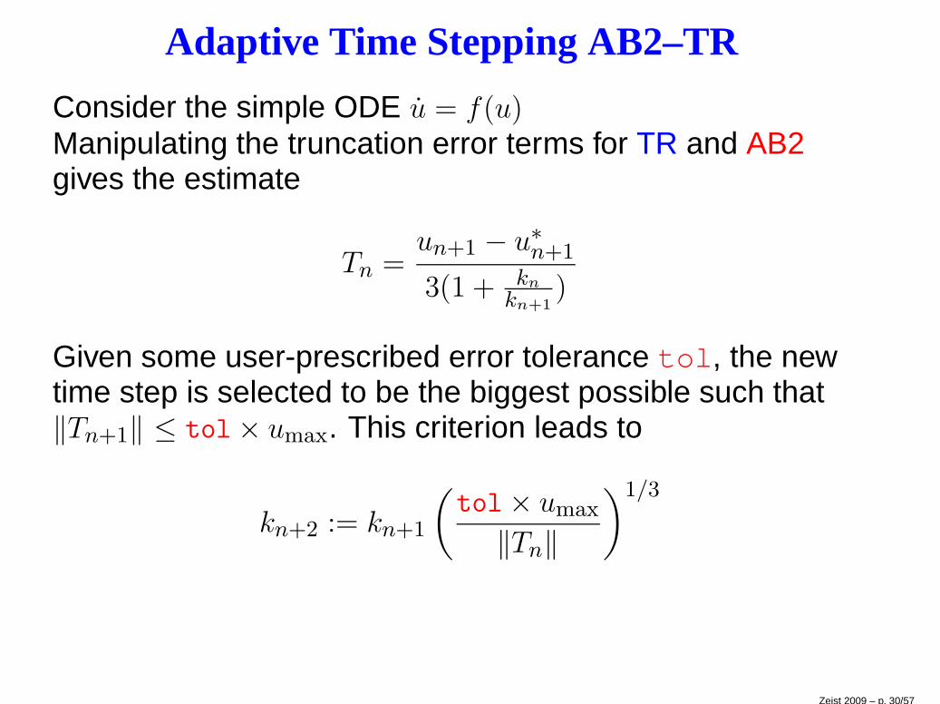
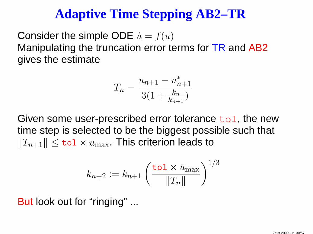
Adaptive Time Stepping AB2–TR

Consider the simple ODE u = f(u)Manipulating the truncation error terms for TR and AB2gives the estimate

Tn =un+1 − u∗n+1

3(1 + kn

kn+1)

Given some user-prescribed error tolerance tol, the newtime step is selected to be the biggest possible such that‖Tn+1‖ ≤ tol× umax. This criterion leads to

kn+2 := kn+1

(tol× umax

‖Tn‖

)1/3

Zeist 2009 – p. 30/57

Adaptive Time Stepping AB2–TR

Consider the simple ODE u = f(u)Manipulating the truncation error terms for TR and AB2gives the estimate

Tn =un+1 − u∗n+1

3(1 + kn

kn+1)

Given some user-prescribed error tolerance tol, the newtime step is selected to be the biggest possible such that‖Tn+1‖ ≤ tol× umax. This criterion leads to

kn+2 := kn+1

(tol× umax

‖Tn‖

)1/3

But look out for “ringing” ...

Zeist 2009 – p. 30/57

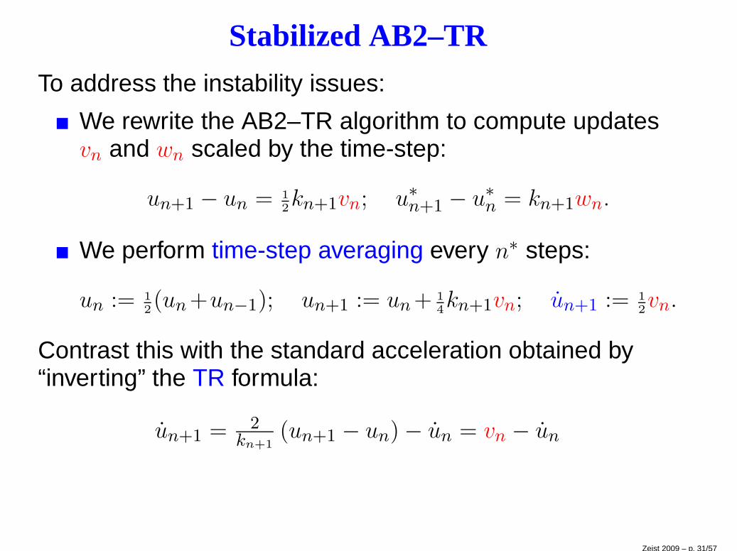
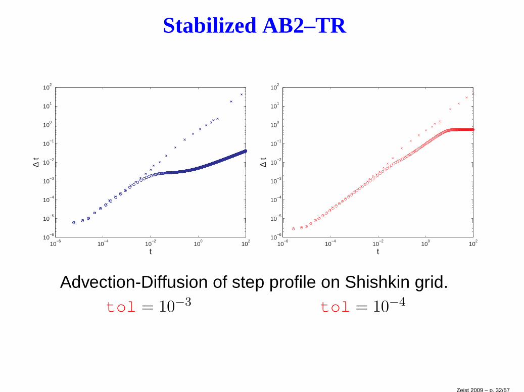
Stabilized AB2–TR

To address the instability issues:

We rewrite the AB2–TR algorithm to compute updatesvn and wn scaled by the time-step:

un+1 − un = 1

2kn+1vn; u∗n+1 − u∗n = kn+1wn.

We perform time-step averaging every n∗ steps:

un := 1

2(un +un−1); un+1 := un + 1

4kn+1vn; un+1 := 1

2vn.

Contrast this with the standard acceleration obtained by“inverting” the TR formula:

un+1 = 2kn+1

(un+1 − un) − un = vn − un

Zeist 2009 – p. 31/57

Stabilized AB2–TR

10−6

10−4

10−2

100

102

10−6

10−5

10−4

10−3

10−2

10−1

100

101

102

∆ t

t10

−610

−410

−210

010

210

−6

10−5

10−4

10−3

10−2

10−1

100

101

102

∆ t

t

Advection-Diffusion of step profile on Shishkin grid.tol = 10−3 tol = 10−4

Zeist 2009 – p. 32/57

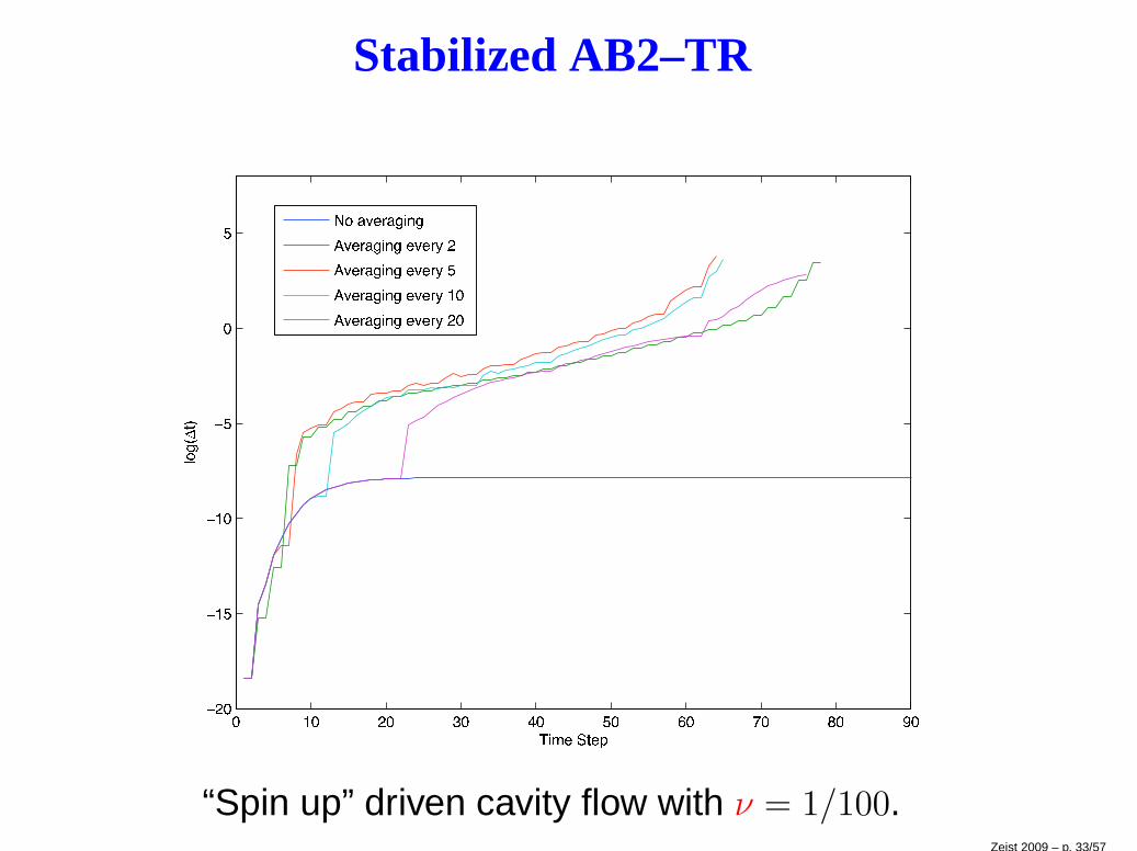
Stabilized AB2–TR

“Spin up” driven cavity flow with ν = 1/100.Zeist 2009 – p. 33/57

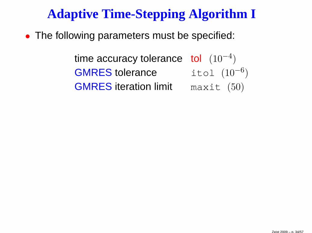
Adaptive Time-Stepping Algorithm I

• The following parameters must be specified:

time accuracy tolerance tol (10−4)

GMRES tolerance itol (10−6)

GMRES iteration limit maxit (50)

Zeist 2009 – p. 34/57

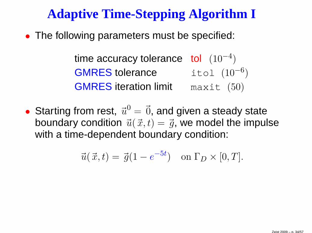
Adaptive Time-Stepping Algorithm I

• The following parameters must be specified:

time accuracy tolerance tol (10−4)

GMRES tolerance itol (10−6)

GMRES iteration limit maxit (50)

• Starting from rest, ~u0 = ~0, and given a steady stateboundary condition ~u(~x, t) = ~g, we model the impulsewith a time-dependent boundary condition:

~u(~x, t) = ~g(1 − e−5t) on ΓD × [0, T ].

Zeist 2009 – p. 34/57

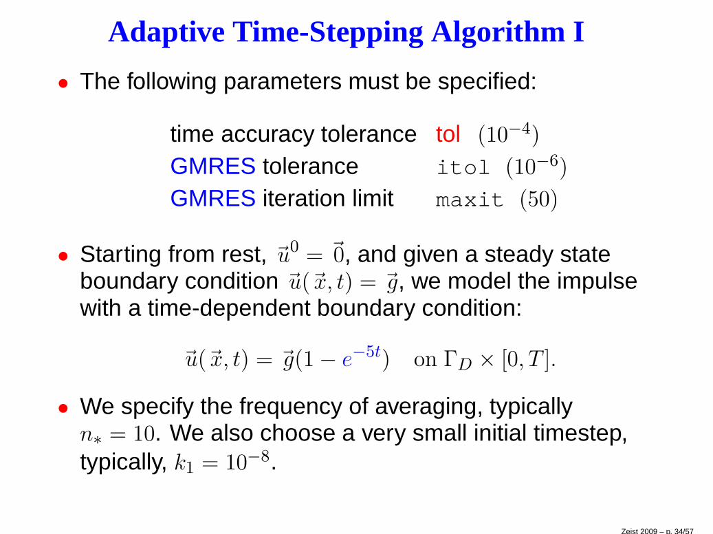
Adaptive Time-Stepping Algorithm I

• The following parameters must be specified:

time accuracy tolerance tol (10−4)

GMRES tolerance itol (10−6)

GMRES iteration limit maxit (50)

• Starting from rest, ~u0 = ~0, and given a steady stateboundary condition ~u(~x, t) = ~g, we model the impulsewith a time-dependent boundary condition:

~u(~x, t) = ~g(1 − e−5t) on ΓD × [0, T ].

• We specify the frequency of averaging, typicallyn∗ = 10. We also choose a very small initial timestep,typically, k1 = 10−8.

Zeist 2009 – p. 34/57

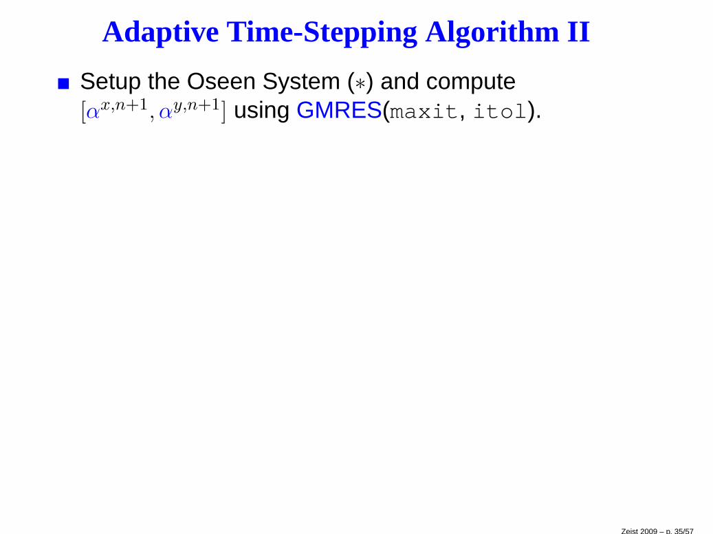
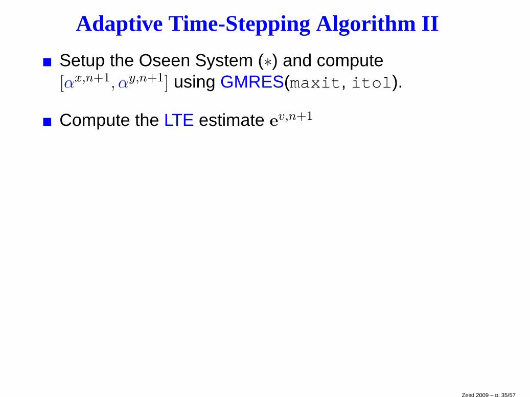
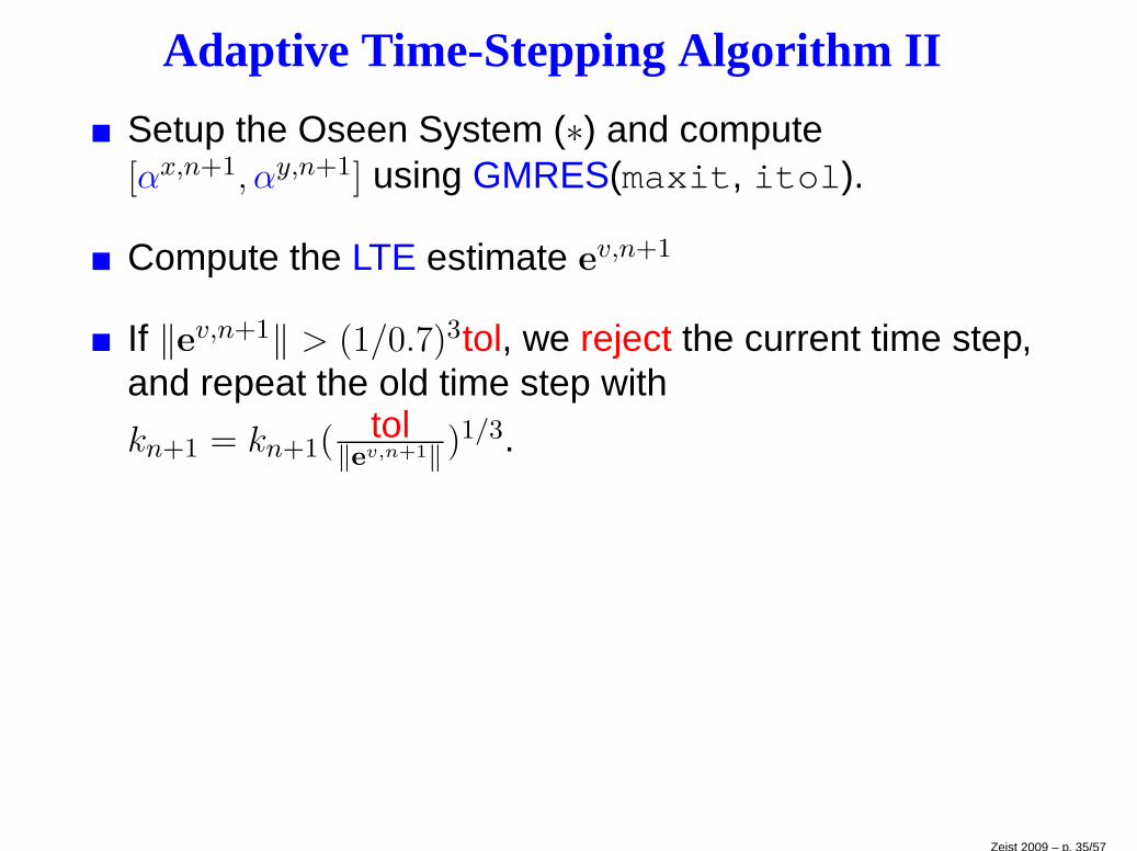
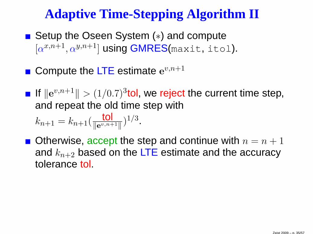
Adaptive Time-Stepping Algorithm II

Setup the Oseen System (∗) and compute[αx,n+1, αy,n+1] using GMRES(maxit, itol).

Zeist 2009 – p. 35/57

Adaptive Time-Stepping Algorithm II

Setup the Oseen System (∗) and compute[αx,n+1, αy,n+1] using GMRES(maxit, itol).

Compute the LTE estimate ev,n+1

Zeist 2009 – p. 35/57

Adaptive Time-Stepping Algorithm II

Setup the Oseen System (∗) and compute[αx,n+1, αy,n+1] using GMRES(maxit, itol).

Compute the LTE estimate ev,n+1

If ‖ev,n+1‖ > (1/0.7)3tol, we reject the current time step,and repeat the old time step with

kn+1 = kn+1(tol

‖ev,n+1‖ )1/3.

Zeist 2009 – p. 35/57

Adaptive Time-Stepping Algorithm II

Setup the Oseen System (∗) and compute[αx,n+1, αy,n+1] using GMRES(maxit, itol).

Compute the LTE estimate ev,n+1

If ‖ev,n+1‖ > (1/0.7)3tol, we reject the current time step,and repeat the old time step with

kn+1 = kn+1(tol

‖ev,n+1‖ )1/3.

Otherwise, accept the step and continue with n = n+ 1and kn+2 based on the LTE estimate and the accuracytolerance tol.

Zeist 2009 – p. 35/57

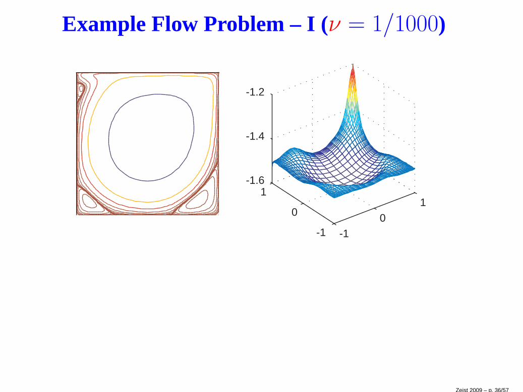
Example Flow Problem – I (ν = 1/1000)

-10

1

-1

0

1-1.6

-1.4

-1.2

Zeist 2009 – p. 36/57

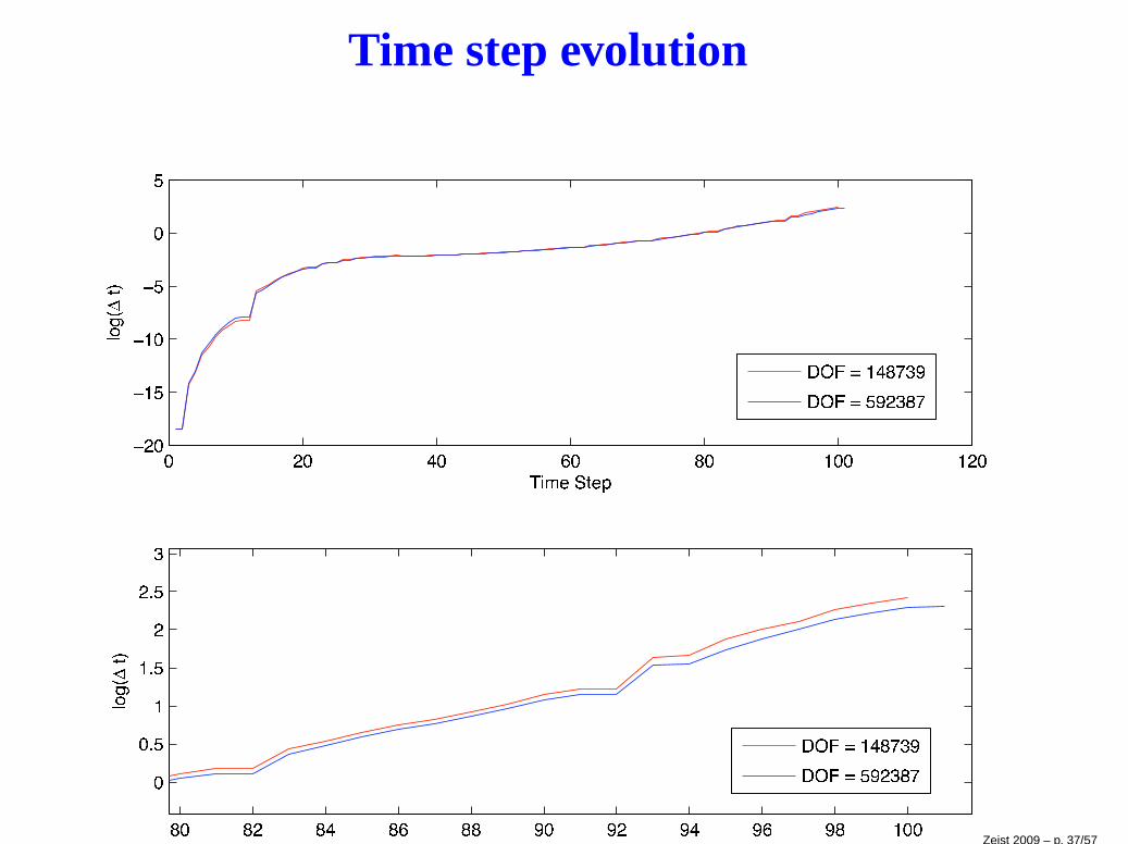
Time step evolution

Zeist 2009 – p. 37/57

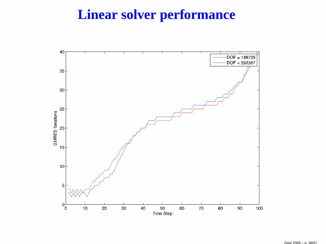
Linear solver performance

Zeist 2009 – p. 38/57

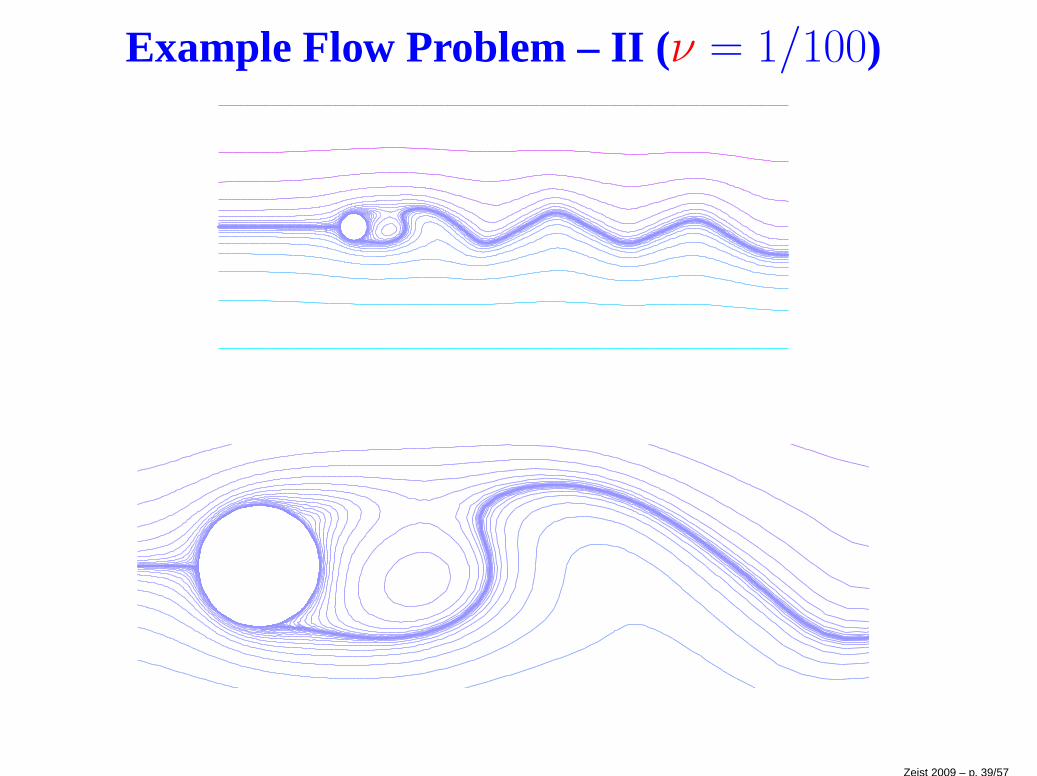
Example Flow Problem – II (ν = 1/100)

Zeist 2009 – p. 39/57

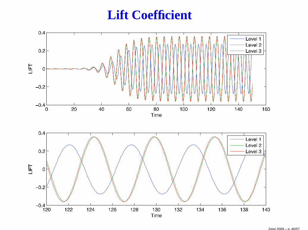
Lift Coefficient

Zeist 2009 – p. 40/57

Time step evolution

Zeist 2009 – p. 41/57

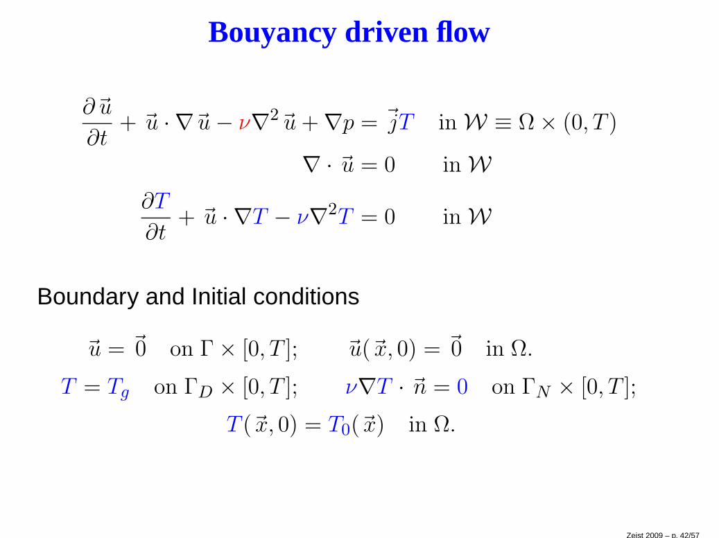
Bouyancy driven flow

∂~u

∂t+ ~u · ∇~u− ν∇2~u+ ∇p = ~jT in W ≡ Ω × (0, T )

∇ · ~u = 0 in W∂T

∂t+ ~u · ∇T − ν∇2T = 0 in W

Boundary and Initial conditions

~u = ~0 on Γ × [0, T ]; ~u(~x, 0) = ~0 in Ω.

T = Tg on ΓD × [0, T ]; ν∇T · ~n = 0 on ΓN × [0, T ];

T (~x, 0) = T0(~x) in Ω.

Zeist 2009 – p. 42/57

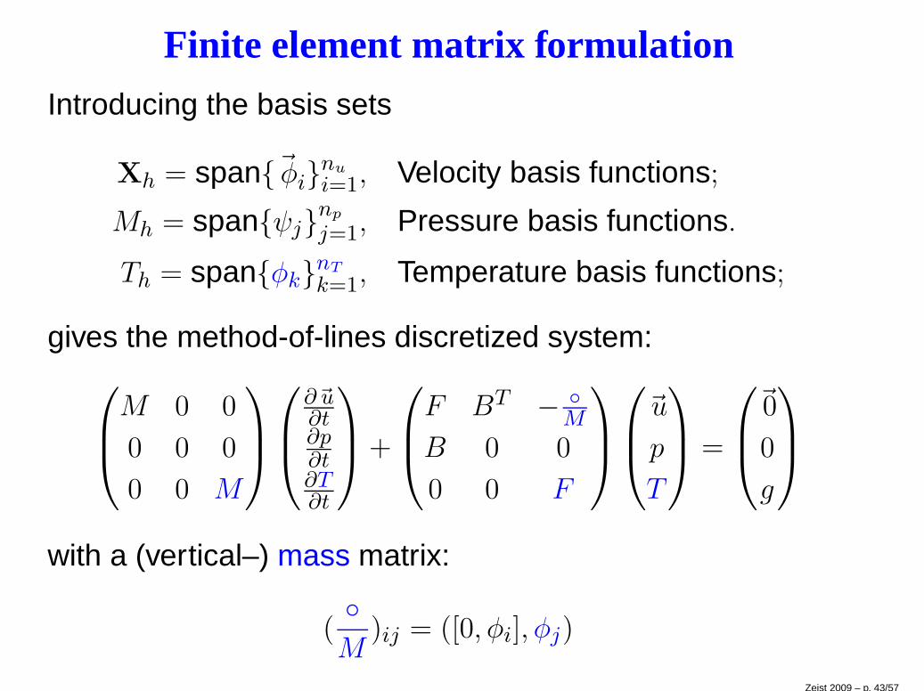
Finite element matrix formulation

Introducing the basis sets

Xh = span~φinu

i=1, Velocity basis functions;

Mh = spanψjnp

j=1, Pressure basis functions.

Th = spanφknT

k=1, Temperature basis functions;

gives the method-of-lines discretized system:

M 0 0

0 0 0

0 0 M

∂~u∂t∂p∂t∂T∂t

+

F BT − M

B 0 0

0 0 F

~u

p

T

=

~0

0

g

with a (vertical–) mass matrix:

(M

)ij = ([0, φi], φj)

Zeist 2009 – p. 43/57

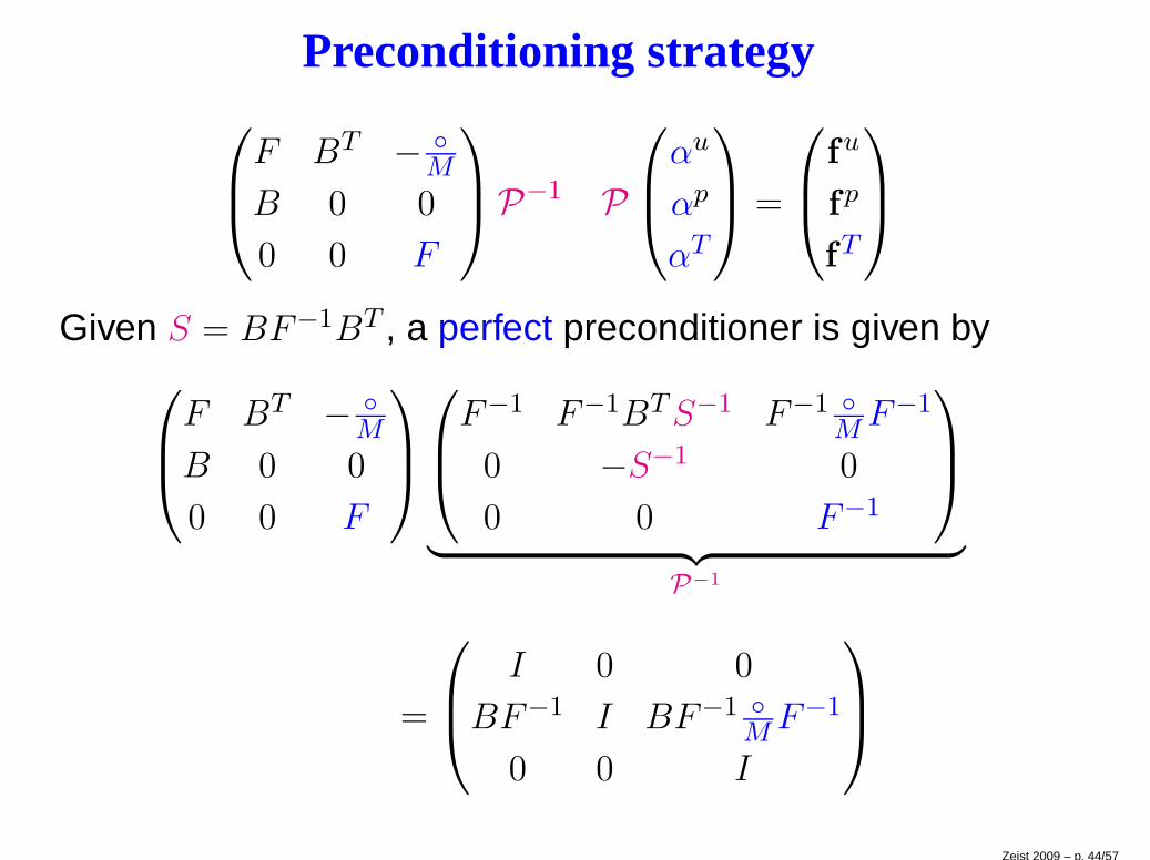
Preconditioning strategy

F BT − M

B 0 0

0 0 F

P−1 P

αu

αp

αT

=

fu

fp

fT

Given S = BF−1BT , a perfect preconditioner is given by

F BT − M

B 0 0

0 0 F

F−1 F−1BTS−1 F−1 MF−1

0 −S−1 0

0 0 F−1

︸ ︷︷ ︸

P−1

=

I 0 0

BF−1 I BF−1 MF−1

0 0 I

Zeist 2009 – p. 44/57

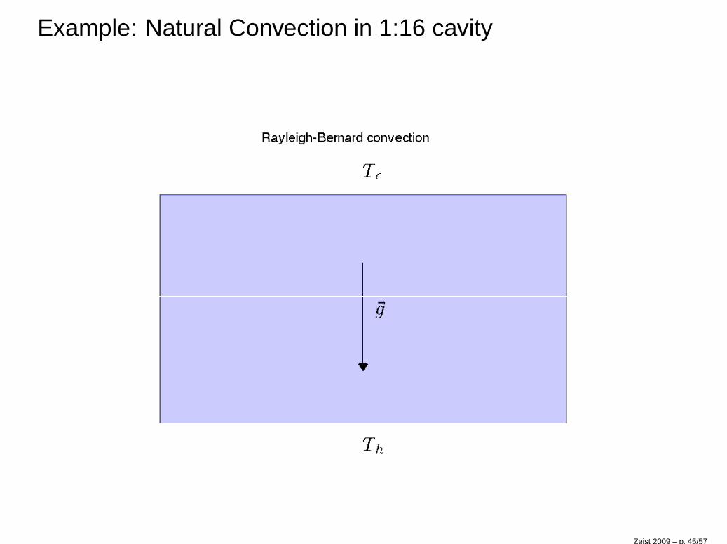
Example: Natural Convection in 1:16 cavity

Zeist 2009 – p. 45/57

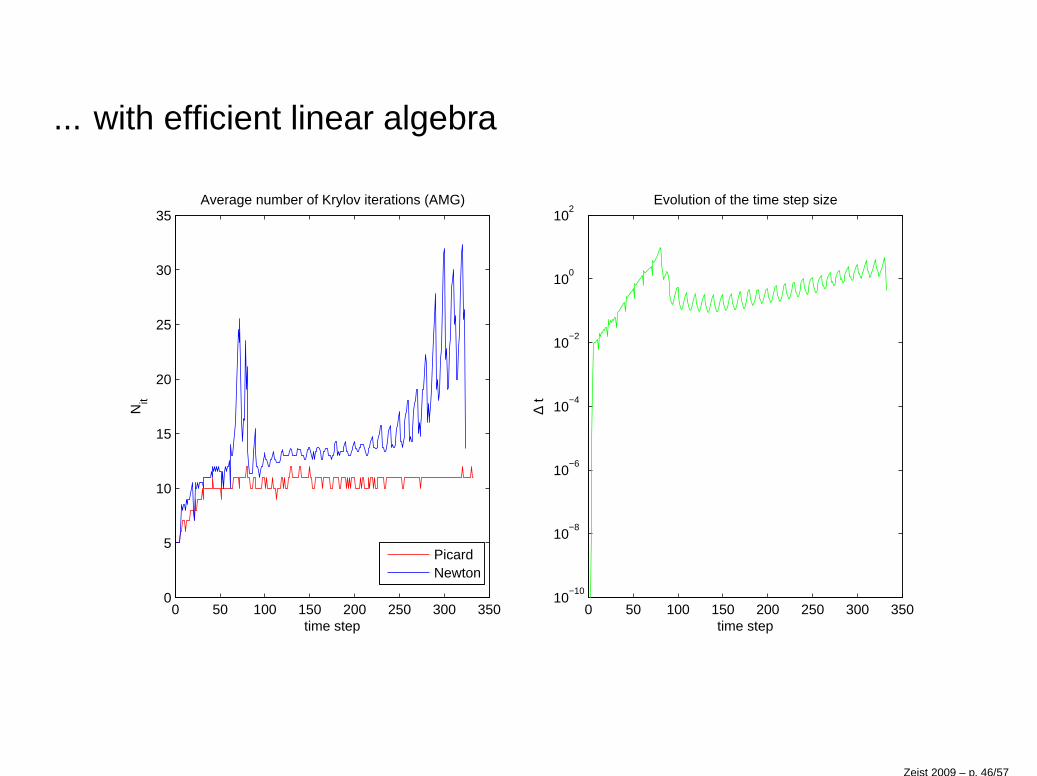
... with efficient linear algebra

0 50 100 150 200 250 300 3500

5

10

15

20

25

30

35

time step

Nit

Average number of Krylov iterations (AMG)

PicardNewton

0 50 100 150 200 250 300 35010

−10

10−8

10−6

10−4

10−2

100

102

time step

∆ t

Evolution of the time step size

Zeist 2009 – p. 46/57

What have we achieved?

• Black-box implementation: few parameters that have tobe estimated a priori.

• Optimal complexity: essentially O(n) flops per iteration,where n is dimension of the discrete system.

• Efficient linear algebra: convergence rate is (essentially)independent of h. Given an appropriate time accuracytolerance convergence is also robust with respect to ν

Zeist 2009 – p. 47/57

ReferencesSemi-Implicit, Fractional-Step, Pressure Projection — I

• A.J. ChorinA numerical method for solving incompressible viscousflow problems, J. Comput. Phys., 2:12–26, 1967.

• J. Kim & P. MoinApplication of a fractional–step method toincompressible Navier–Stokes equations,J. Comput. Phys., 59:308–323, 1985.

• J. Van KanA second–order accurate pressure–correction schemefor viscous incompressible flow,SIAM J. Sci. Stat. Comput., 7(3):870–891, 1986.

• J.B. Bell, P. Colella & H.M. GlazA second–order projection method for theincompressible Navier–Stokes equations,J. Comput. Phys., 85:(2)257–283, 1989.

Zeist 2009 – p. 48/57

Semi-Implicit, Fractional-Step, Pressure Projection — II

• P.M. Gresho, S.T. Chan, R.L. Lee & C.D. UpsonA modified finite element method for solving thetime–dependent, incompressible Navier–Stokesequations. Part 1: Theory,Int. J. Numer. Meth. Fluids, 4:557–598, 1984.

• P.M. Gresho & S.T. ChanOn the theory of semi–implicit projection methods forviscous incompressible flow and its implementation viaa finite element method that also introduces a nearlyconsistent mass matrix. Part 2: Implementation,Int. J. Numer. Meth. Fluids, 11(5):621-660, 1990.

• J.B. PerotAn analysis of the fractional step method,J. Comput. Phys., 108:51–58, 1993.

Zeist 2009 – p. 49/57

Semi-Implicit, Fractional-Step, Pressure Projection — III

• J.–L. GuermondSur l’approximation des équations de Navier–Stokesinstationnaires par une méthode de projection, C.R.Acad. Sci. Paris, 319:887–892, 1994. Serie I.

• R. RannacherThe Navier–Stokes Equations II: Theory and NumericalMethods, Springer–Verlag, Berlin, Germany, 1992.Chap.On Chorin’s projection method for theincompressible Navier–Stokes equations; pp. 167–183;Lecture Notes in Mathematics, Vol. 1530.

Zeist 2009 – p. 50/57

Semi-Implicit, Fractional-Step, Pressure Projection — IV

• W. E & J.–G. LiuProjection method I: Convergence and numericalboundary layers,SIAM J. Numer. Anal., 32(4):1017–1057, 1995.

• W. E & J.–G. LiuVorticity boundary conditions and related issues forfinite difference schemes,J. Comput. Phys., 124:368–382, 1996.

Zeist 2009 – p. 51/57

Semi-Implicit, Fractional-Step, Pressure Projection — V

• J. ShenOn error estimates of some higher order projection andpenalty–projection methods for Navier–Stokesequations, Numer. Math., 62:49–73, 1992.

• J. ShenOn error estimates of the projection methods for theNavier–Stokes equations: Second–order schemes,Math. Comput., 65, 215:1039–1065, 1996.

• A. ProhlAnalysis of Chorin’s projection method for solving theincompressible Navier–Stokes equations, UniversitätHeidelberg, Institut für Angewandte Mathematik, INF294, D–69120 Heidelberg, Germany, 1996.

Zeist 2009 – p. 52/57

Transport Diffusion, Lagrange-Galerkin, Backward Methodof Characteristics — I

• P. HansboThe characteristic streamline diffusion method for thetime–dependent incompressible Navier–Stokesequations, Comput. Meth. Appl. Mech. Eng.,99:171–186, 1992.

• O. PironneauOn the transport–diffusion algorithm and its applicationto the Navier–Stokes equations, Numer. Math.,38:309–332, 1982.

• K.W. Morton, A. Priestley & E. SüliStability of the Lagrange–Galerkin method withnon–exact integration,Math. Model. Numer. Anal., 22:(4)625–653, 1988.

Zeist 2009 – p. 53/57

Transport Diffusion, Lagrange-Galerkin, Backward Methodof Characteristics — II

• A. PriestleyExact projections and the Lagrange–Galerkin method:A realistic alternative to quadrature, J. Comput. Phys.,112:316–333, 1994

• R. BermejoAnalysis of an algorithm for the Galerkin–characteristicmethod, Numer. Math., 60:163–194, 1991.

Zeist 2009 – p. 54/57

Fractional Step, le Θ scheme — I

• M.O. Bristeau, R. Glowinski, B. Mantel,J. Periaux & P. Perrier, Numerical methods forincompressible and compressible Navier–Stokesproblems, Finite Elements in Fluids 6 (R.H. Gallagher,G. Carey, J.T. Oden & O.C. Zienkiewicz, eds),Chichester: Wiley, 1985. pp. 1–40.

• E.J. Dean & R. GlowinskiOn some finite element methods for the numericalsimulation of incompressible viscous flow,Incompressible Computational Fluid Dynamics., (M.D.Gunzburger & R.A. Nicolaides, eds), CambridgeUniversity Press, 1993. pp. 17–65.

Zeist 2009 – p. 55/57

Fractional Step, le Θ scheme — II

• R. RannacherApplications of mathematics in industry and technology,B.G. Teubner, Stuttgart, Germany, 1989. Chap.Numerical analysis of nonstationary fluid flow (asurvey); pp. 34–53; (V.C. Boffi & H. Neunzert, eds).

• R. RannacherNavier–Stokes equations: theory and numericalmethods, Springer–Verlag, Berlin, Germany, 1990.Chap. On the numerical analysis of the non–stationaryNavier–Stokes equations; pp. 180–193; (J. Heywood etal., eds).

Zeist 2009 – p. 56/57

Fractional Step, le Θ scheme — III

• S. TurekA comparative study of some time–stepping techniquesfor the incompressible Navier–Stokes equations: Fromfully implicit nonlinear schemes to semi–implicitprojection methods, Int. J. Numer. Meth. Fluids,22(10):987–1012, 1996.

• A. Smith & D.J. SilvesterImplicit algorithms and their linearization for thetransient incompressible Navier–Stokes equations,IMA J. Numer. Anal. 17: 527–545, 1997.

Zeist 2009 – p. 57/57