Approximating models

Nancy Reid, University of Toronto

Oxford, February 6

www.utstat.utoronto.reid/research

1

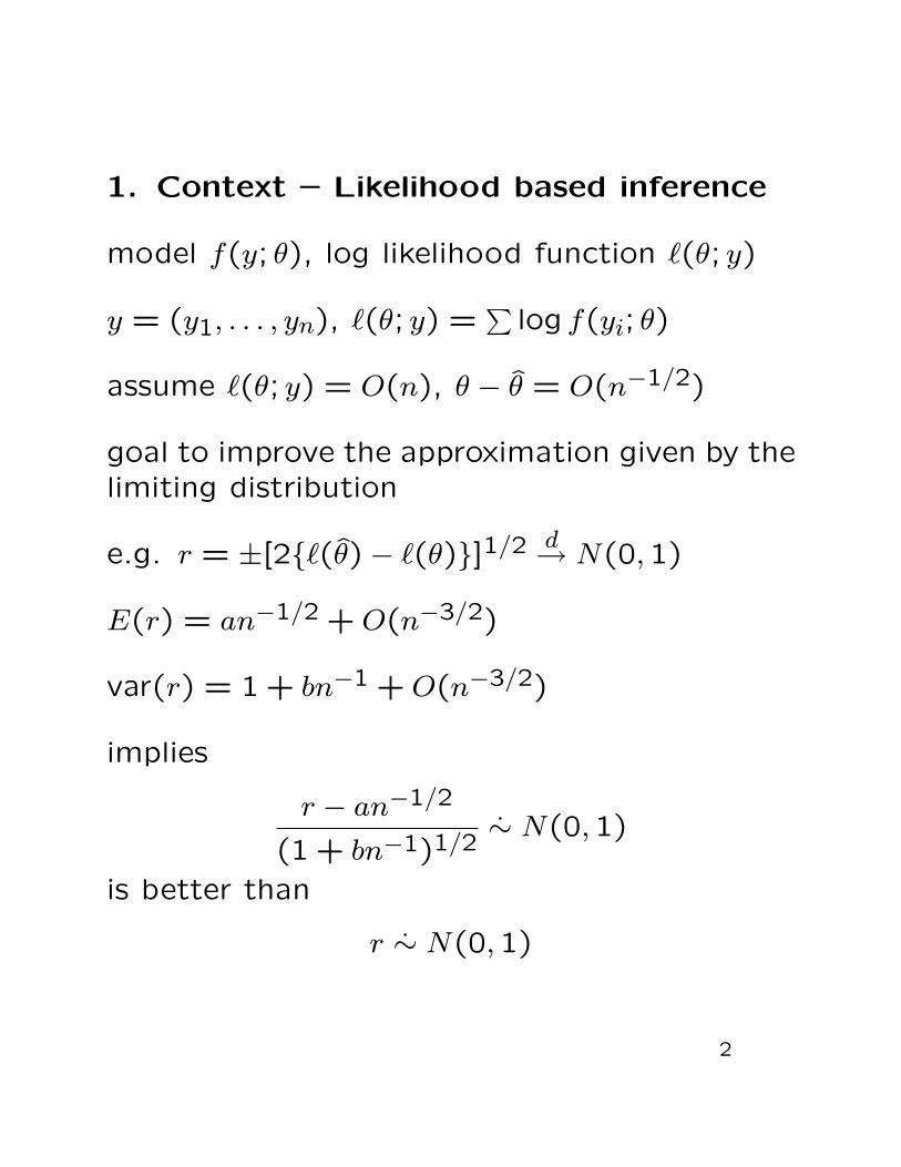
1. Context – Likelihood based inference

model f(y; θ), log likelihood function "(θ; y)

y = (y1, . . . , yn), "(θ; y) =∑

log f(yi; θ)

assume "(θ; y) = O(n), θ − θ = O(n−1/2)

goal to improve the approximation given by thelimiting distribution

e.g. r = ±[2{"(θ)− "(θ)}]1/2 d→ N(0,1)

E(r) = an−1/2 + O(n−3/2)

var(r) = 1 + bn−1 + O(n−3/2)

implies

r − an−1/2

(1 + bn−1)1/2.∼ N(0,1)

is better than

r.∼ N(0,1)

2

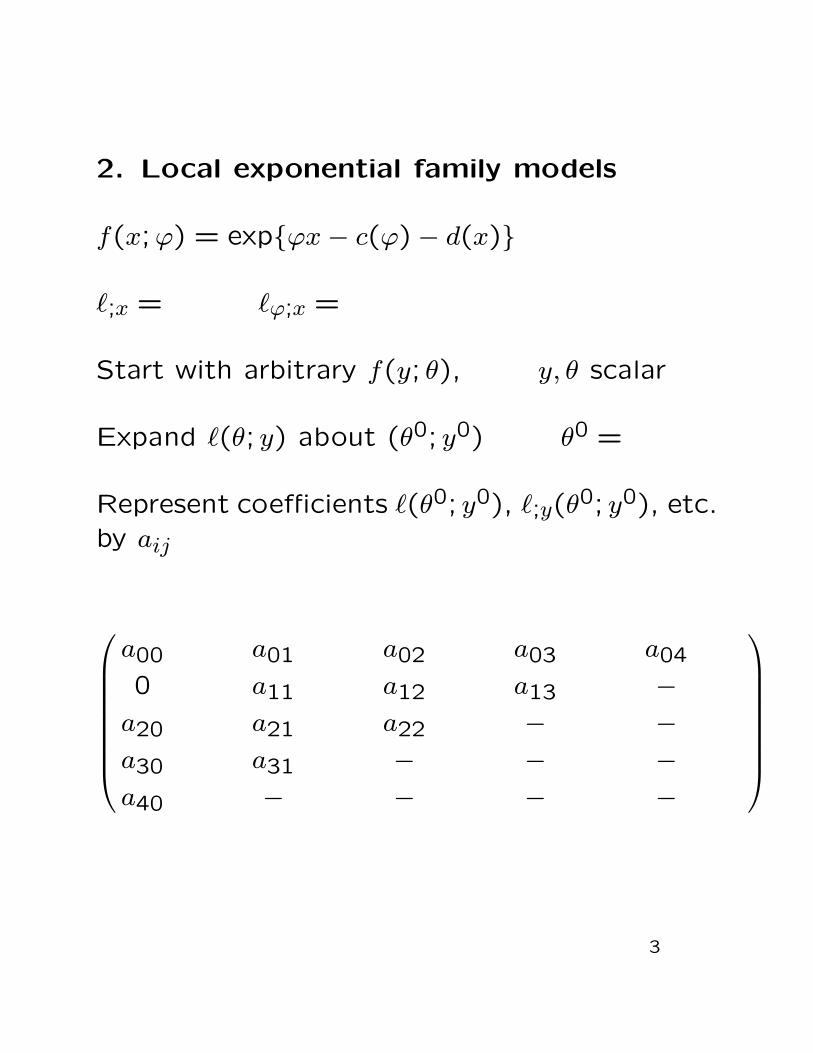
2. Local exponential family models

f(x;ϕ) = exp{ϕx− c(ϕ)− d(x)}

";x = "ϕ;x =

Start with arbitrary f(y; θ), y, θ scalar

Expand "(θ; y) about (θ0; y0) θ0 =

Represent coefficients "(θ0; y0), ";y(θ0; y0), etc.by aij

a00 a01 a02 a03 a04

0 a11 a12 a13 −a20 a21 a22 − −a30 a31 − − −a40 − − − −

3

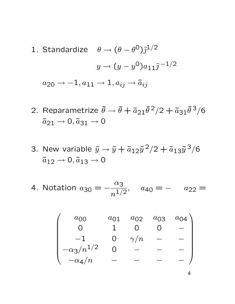
1. Standardize θ → (θ − θ0)1/2

y → (y − y0)a11−1/2

a20 → −1, a11 → 1, aij → aij

2. Reparametrize θ → θ + a21θ 2/2 + a31θ 3/6a21 → 0, a31 → 0

3. New variable y → y + a12y 2/2 + a13y 3/6a12 → 0, a13 → 0

4. Notation a30 = − α3

n1/2, a40 = − a22 =

a00 a01 a02 a03 a04

0 1 0 0 −−1 0 γ/n − −

−α3/n1/2 0 − − −−α4/n − − − −

4

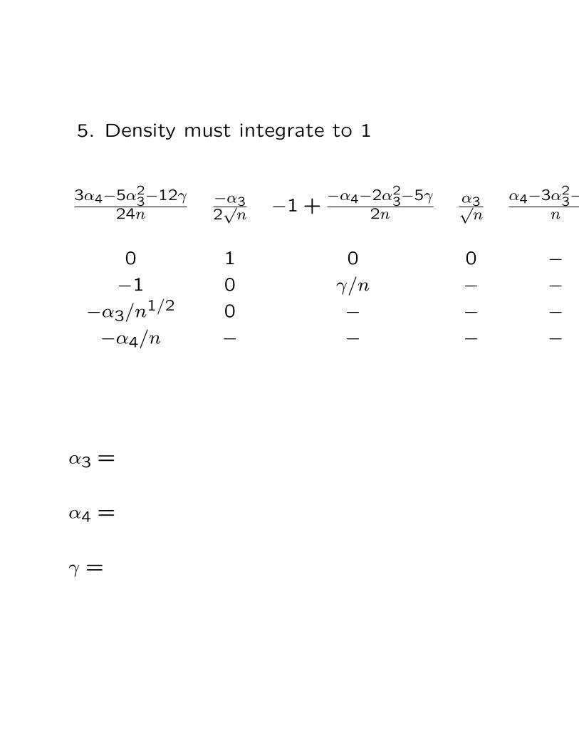
5. Density must integrate to 1

3α4−5α23−12γ

24n−α32√

n −1 +−α4−2α2

3−5γ2n

α3√n

α4−3α23−6γ

n

0 1 0 0 −−1 0 γ/n − −

−α3/n1/2 0 − − −−α4/n − − − −

α3 =

α4 =

γ =

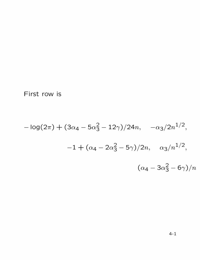
First row is

− log(2π) + (3α4 − 5α23 − 12γ)/24n, −α3/2n1/2,

−1 + (α4 − 2α23 − 5γ)/2n, α3/n1/2,

(α4 − 3α23 − 6γ)/n

4-1

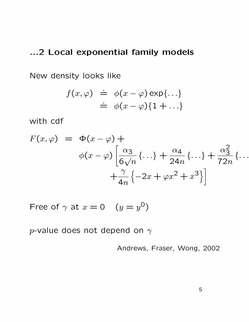
...2 Local exponential family models

New density looks like

f(x, ϕ).= φ(x− ϕ) exp{. . .}.= φ(x− ϕ){1 + . . .}

with cdf

F (x, ϕ) = Φ(x− ϕ) +

φ(x− ϕ)

[α3

6√

n{. . .} +

α4

24n{. . .}+

α23

72n{. . .}

+γ

4n

{−2x + ϕx2 + x3

}]

Free of γ at x = 0 (y = y0)

p-value does not depend on γ

Andrews, Fraser, Wong, 2002

5

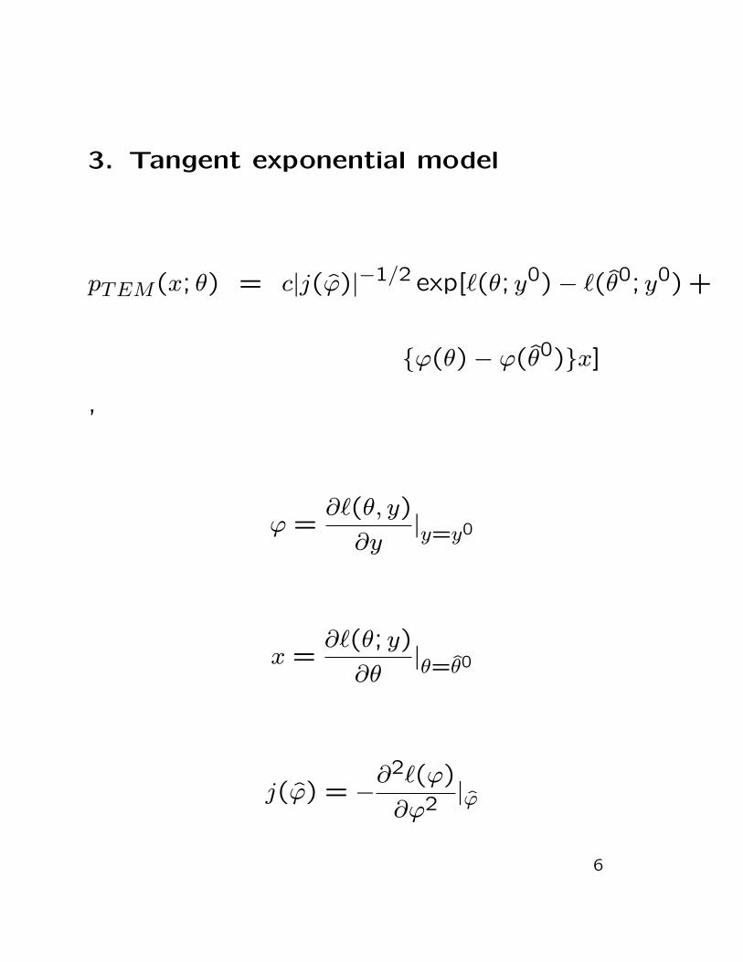
3. Tangent exponential model

pTEM(x; θ) = c|j(ϕ)|−1/2 exp["(θ; y0)− "(θ0; y0) +

{ϕ(θ)− ϕ(θ0)}x],

ϕ =∂"(θ, y)

∂y|y=y0

x =∂"(θ; y)

∂θ|θ=θ0

j(ϕ) = −∂2"(ϕ)

∂ϕ2 |ϕ

6

"(θ; y0) is first column (ignoring (0,0) entry)ϕ(θ) is second column (ignoring (0,1) entry)

These 2 columns determine the rest of the ar-ray, except the γ/n term

Easy to use pTEM to get a p-value (saddlepointtype approximation)

6-1

...3 Tangent exponential model

How to get a scalar variable y? Condition onan (approximate) ancillary, so ";y is taken forfixed ancillary a(y).

This can be computed by finding a vector V =(V1, . . . , Vn)T tangent to the ancillary at y0:

ϕ(θ) = ";V (θ; y)|y0 =∑

";yi(θ; y0i )Vi

Example

yi ∼ f(yi − µ) ai = yi − µ, say, Vi = 1

ϕ(θ) =∑ ∂ log f(yi − µ)

∂yi|y0 = −"θ(θ; y0)

7

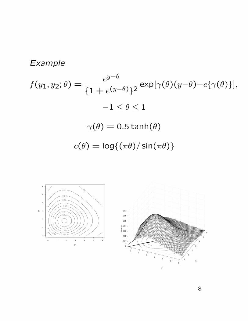
Example

f(y1, y2; θ) =ey−θ

{1 + e(y−θ)}2 exp[γ(θ)(y−θ)−c{γ(θ)}],

−1 ≤ θ ≤ 1

γ(θ) = 0.5 tanh(θ)

c(θ) = log{(πθ)/ sin(πθ)}

y1

y2

0 1 2 3 4 5 6

01

23

45

6

01

23

45

60

1

2

3

4

5

6

0

0.01

0.02

0.03

0.04

0.05

0.06

0.07

y2

y1

de

nsi

ty

8

...3 Tangent exponential model Vector θ?Use the same approach, now

V = (V 1, V 2, . . . , V n)T

V i is 1× d, ";V (θ) is also 1× d

Example

yi = xTi β + σei

V i = (xTi ei)

Example

yi = µi(β) + σei

V i = {µ′i(β) ei}Inference re nuisance parameters uses pTEM

twice to get a marginal distribution

Example House price data (Srivastava and Sen);4 covariates, 26 observations, model

yi = xTi β + σei, ei ∼ t5

9

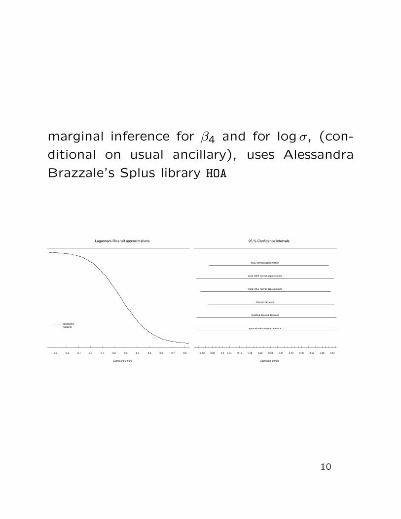
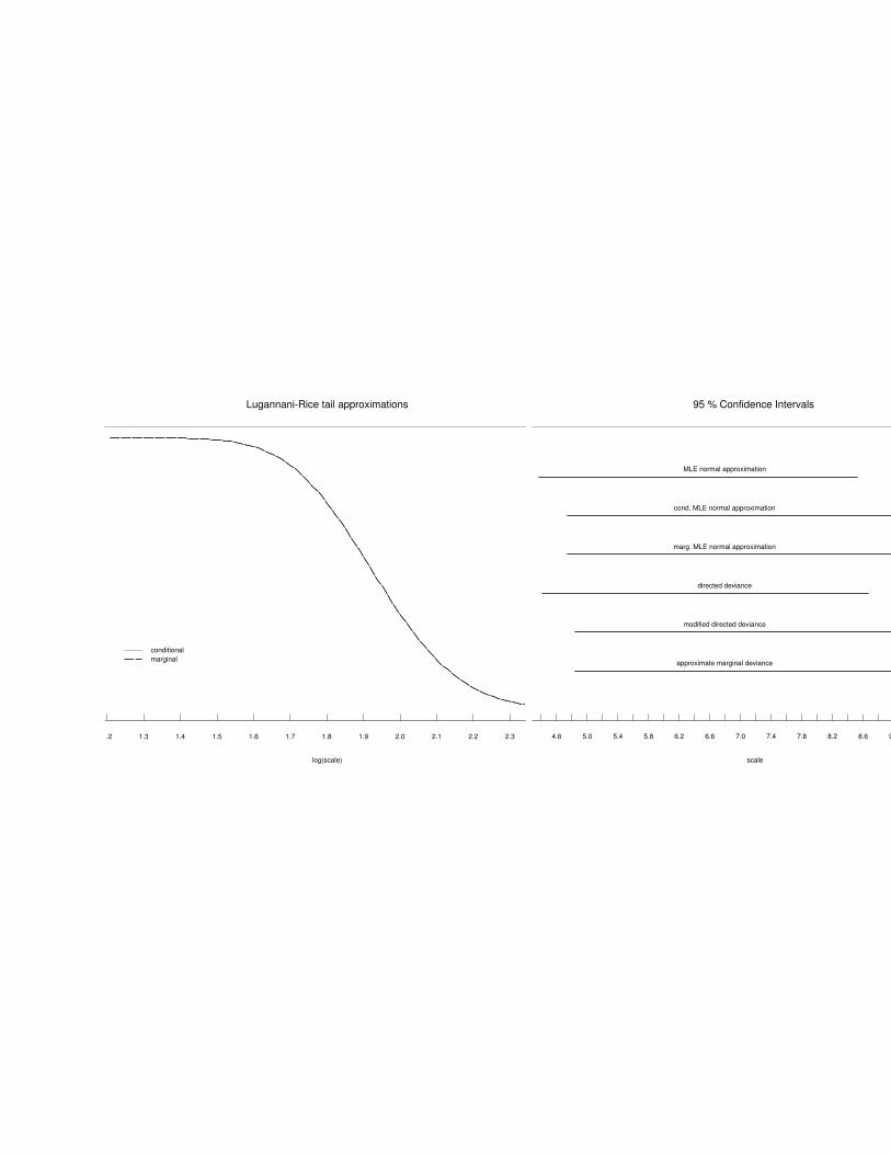
marginal inference for β4 and for logσ, (con-ditional on usual ancillary), uses AlessandraBrazzale’s Splus library HOA

-0.4 -0.3 -0.2 -0.1 0.0 0.1 0.2 0.3 0.4 0.5 0.6 0.7 0.8 0.9

0.0

0.1

0.2

0.3

0.4

0.5

0.6

0.7

0.8

0.9

1.0

Lugannani-Rice tail approximations

Coefficient of front

tail

appr

oxim

atio

n

conditionalmarginal

-0.18 -0.12 -0.06 0.0 0.04 0.10 0.16 0.22 0.28 0.34 0.40 0.46 0.52 0.58 0.64 0.70

0

2

4

6

95 % Confidence Intervals

Coefficient of front

conf

iden

ce in

terv

als

directed deviance

modified directed deviance

approximate marginal deviance

MLE normal approximation

cond. MLE normal approximation

marg. MLE normal approximation

10

-0.20 -0.10 0.0 0.05 0.10 0.15 0.20 0.25 0.30 0.35 0.40 0.45 0.50 0.55 0.60 0.65 0.70 0.75

-3.0

-2.8

-2.6

-2.4

-2.2

-2.0

-1.8

-1.6

-1.4

-1.2

-1.0

-0.8

-0.6

-0.4

-0.2

0.0

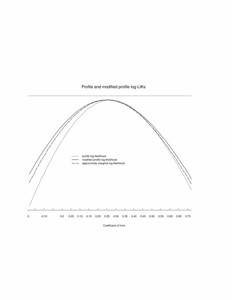
Profile and modified profile log-LIKs

Coefficient of front

log

likel

ihoo

d

profile log-likelihoodmodified profile log-likelihoodapproximate marginal log-likelihood

1.2 1.3 1.4 1.5 1.6 1.7 1.8 1.9 2.0 2.1 2.2 2.3 2.4

0.0

0.1

0.2

0.3

0.4

0.5

0.6

0.7

0.8

0.9

1.0

Lugannani-Rice tail approximations

log(scale)

tail

appr

oxim

atio

n

conditionalmarginal

4.2 4.6 5.0 5.4 5.8 6.2 6.6 7.0 7.4 7.8 8.2 8.6 9.0 9.4 9.8 10.2

0

2

4

6

95 % Confidence Intervals

scale

conf

iden

ce in

terv

als

directed deviance

modified directed deviance

approximate marginal deviance

MLE normal approximation

cond. MLE normal approximation

marg. MLE normal approximation

1.50 1.55 1.60 1.65 1.70 1.75 1.80 1.85 1.90 1.95 2.00 2.05 2.10 2.15 2.20 2.25

-3.0

-2.8

-2.6

-2.4

-2.2

-2.0

-1.8

-1.6

-1.4

-1.2

-1.0

-0.8

-0.6

-0.4

-0.2

0.0

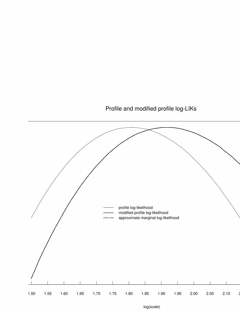
Profile and modified profile log-LIKs

log(scale)

log

likel

ihoo

d

profile log-likelihoodmodified profile log-likelihoodapproximate marginal log-likelihood

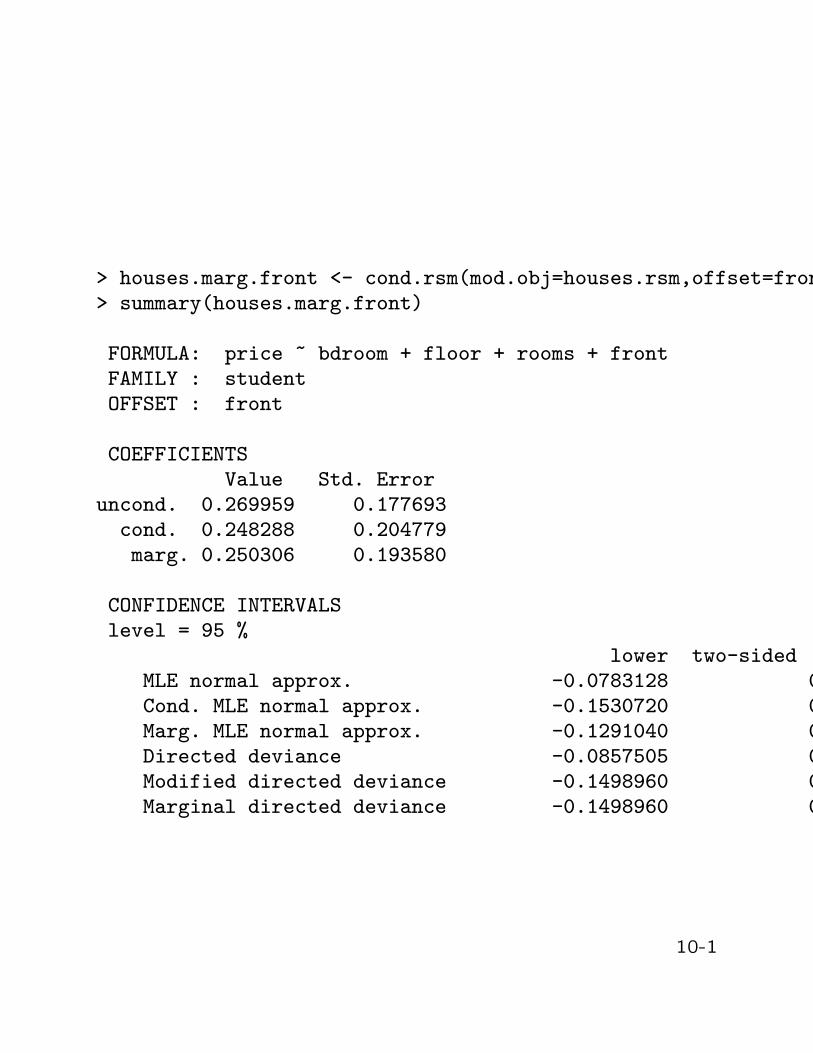
> houses.marg.front <- cond.rsm(mod.obj=houses.rsm,offset=front)> summary(houses.marg.front)

FORMULA: price ~ bdroom + floor + rooms + frontFAMILY : studentOFFSET : front

COEFFICIENTSValue Std. Error

uncond. 0.269959 0.177693cond. 0.248288 0.204779marg. 0.250306 0.193580

CONFIDENCE INTERVALSlevel = 95 %

lower two-sided upperMLE normal approx. -0.0783128 0.618231Cond. MLE normal approx. -0.1530720 0.649647Marg. MLE normal approx. -0.1291040 0.629716Directed deviance -0.0857505 0.654045Modified directed deviance -0.1498960 0.699837Marginal directed deviance -0.1498960 0.699837

10-1

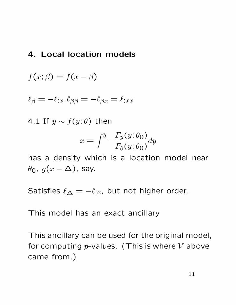
4. Local location models

f(x;β) = f(x− β)

"β = −";x "ββ = −"βx = ";xx

4.1 If y ∼ f(y; θ) then

x =∫ y−Fy(y; θ0)

Fθ(y; θ0)dy

has a density which is a location model nearθ0, g(x−∆), say.

Satisfies "∆ = −";x, but not higher order.

This model has an exact ancillary

This ancillary can be used for the original model,for computing p-values. (This is where V abovecame from.)

11

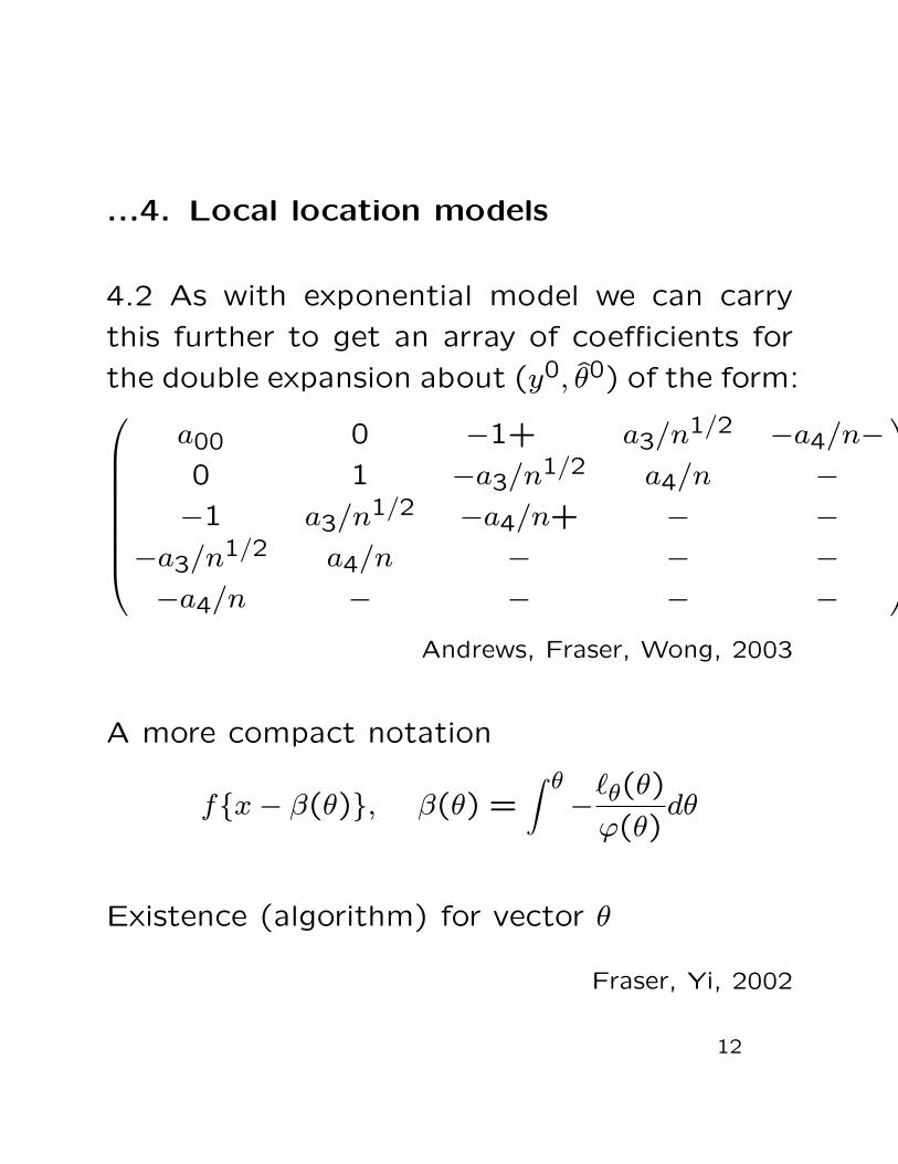
...4. Local location models

4.2 As with exponential model we can carrythis further to get an array of coefficients forthe double expansion about (y0, θ0) of the form:

a00 0 −1+ a3/n1/2 −a4/n−0 1 −a3/n1/2 a4/n −−1 a3/n1/2 −a4/n+ − −

−a3/n1/2 a4/n − − −−a4/n − − − −

Andrews, Fraser, Wong, 2003

A more compact notation

f{x− β(θ)}, β(θ) =∫ θ−"θ(θ)

ϕ(θ)dθ

Existence (algorithm) for vector θ

Fraser, Yi, 2002

12

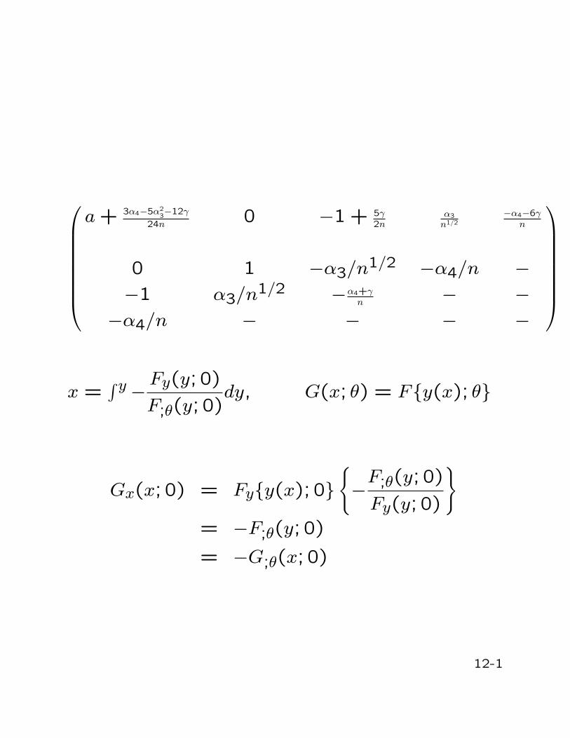
a + 3α4−5α23−12γ

24n0 −1 + 5γ

2nα3

n1/2−α4−6γ

n

0 1 −α3/n1/2 −α4/n −−1 α3/n1/2 −α4+γ

n− −

−α4/n − − − −

x =∫ y−Fy(y; 0)

F;θ(y; 0)dy, G(x; θ) = F{y(x); θ}

Gx(x; 0) = Fy{y(x); 0}{−F;θ(y; 0)

Fy(y; 0)

}= −F;θ(y; 0)

= −G;θ(x; 0)

12-1

...4 Local location model

Bayesian analysis of location model uses flatprior for location parameter, in our case

π(θ) ∝ dβ(θ)

and this will give posterior p-values equal tothose from tangent exponential model

to O(n−3/2) if non-location term γ = 0,

to O(n−1) if γ )= 0

With nuisance parameters, can only obtain ’strongmatching’ priors for a single parameter of in-terest, using

π(ψ, λψ) ∝∣∣∣∣∣∂ψ

∂β

∣∣∣∣∣−1

(ψ,λψ)× |jλλ(θψ)|

|ϕλ(θψ)|Fraser & Reid, 2003

13

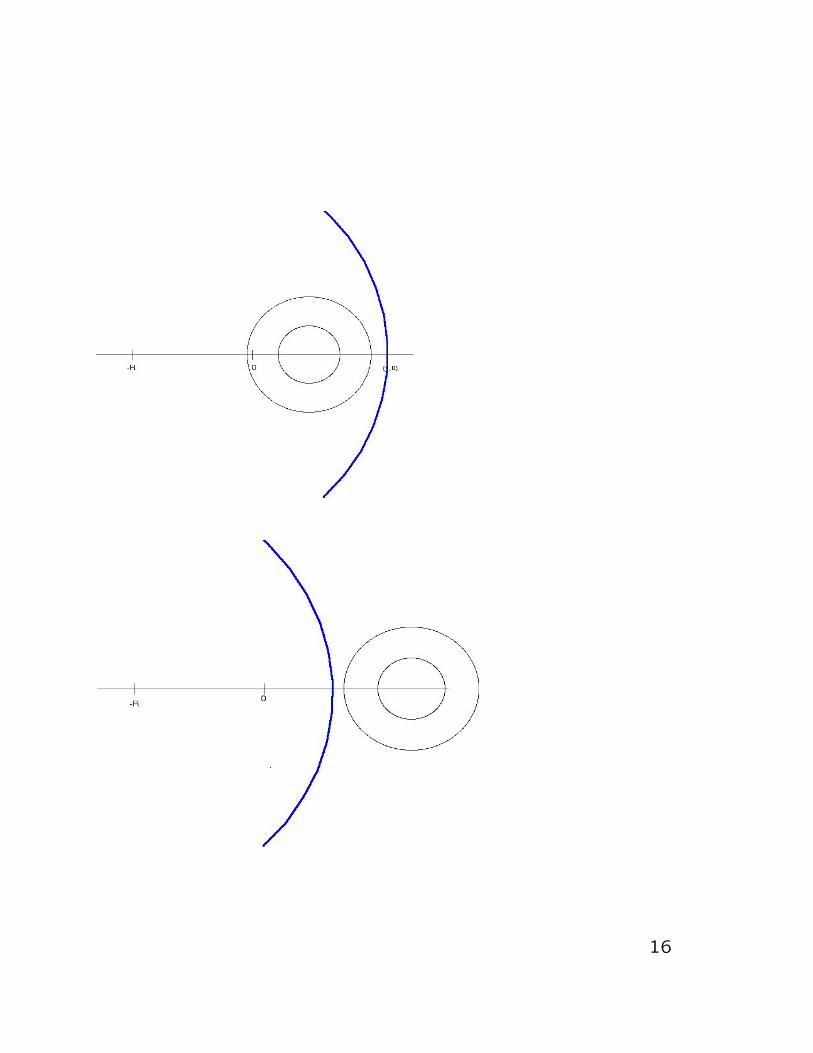
Example Location model with curved parame-ter of interest

Y1 ∼ N(θ1,1), Y2 ∼ N(θ2,1) independent

ψ2 = (R + θ1)2 + θ22; R known

r2 =√{(R + y1)2 + y2

2}

Bayesian posterior under usual flat prior (θ1, θ2|y) ∼N(y1, y2)

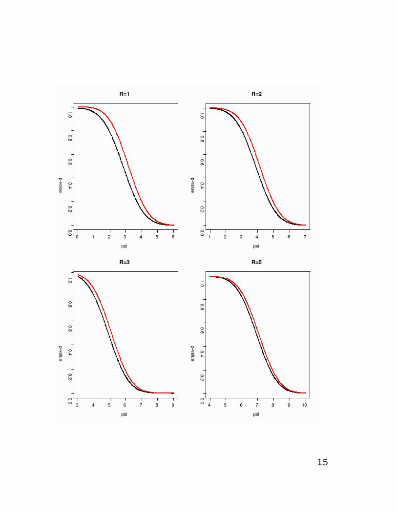
frequentist p-value (marginal) Pr{r ≤ r0;ψ0)

Bayesian p-value Pr{ψ ≥ ψ0|y)

Will be quite different:

matching prior using information adjustmentgives π(θ) ∝ r

ψ

14

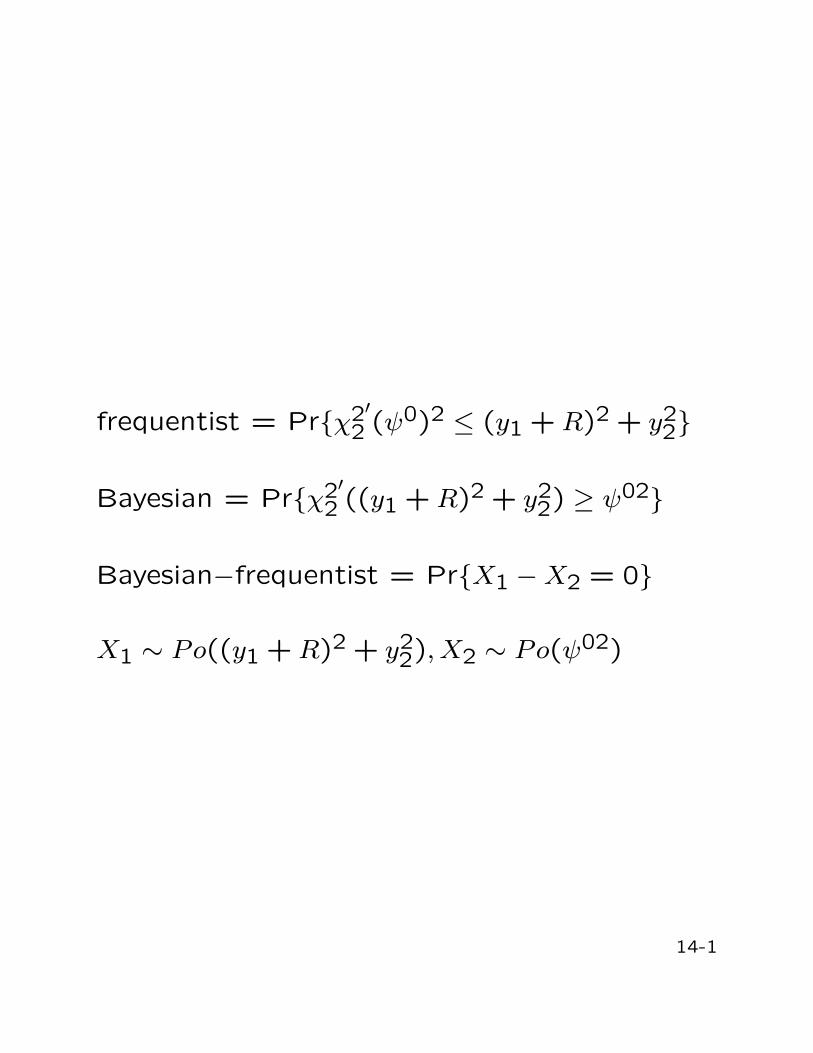
frequentist = Pr{χ2′2 (ψ0)2 ≤ (y1 + R)2 + y2

2}

Bayesian = Pr{χ2′2 ((y1 + R)2 + y2

2) ≥ ψ02}

Bayesian−frequentist = Pr{X1 −X2 = 0}

X1 ∼ Po((y1 + R)2 + y22), X2 ∼ Po(ψ02)

14-1

0 1 2 3 4 5 6

0.00.2

0.40.6

0.81.0

R=1

psi

p-value

1 2 3 4 5 6 7

0.00.2

0.40.6

0.81.0

R=2

psi

p-value

3 4 5 6 7 8 9

0.00.2

0.40.6

0.81.0

R=3

psi

p-value

4 5 6 7 8 9 10

0.00.2

0.40.6

0.81.0

R=5

psi

p-value

15

16

References

Andrews, D.A., Fraser, D.A.S., Wong, A. Computation of distri-bution functions from likelihood information near observed data.

Brazzale, A. http://www.isib.cnr.it/ brazzale

Fraser, D.A.S., Reid, N. Strong matching of frequentist and Bayesianparametric inference.

Fraser, D.A.S., Yi, G. Location reparametrization and default priorsfor statistical analyses.

Reid, N. Asymptotics and the theory of inference.

17