A Numerical Analysis Perspective on Deep Neural...
29
Lars Ruthotto Numerical Analysis of DNNs @ IPAM, 2019 A Numerical Analysis Perspective on Deep Neural Networks Machine Learning for Physics and the Physics of Learning Los Angeles, September, 2019 Lars Ruthotto Departments of Mathematics and Computer Science, Emory University [email protected] @lruthotto Title Intro Rev Black-Box D→O cond Σ 1
Transcript of A Numerical Analysis Perspective on Deep Neural...
Lars Ruthotto Numerical Analysis of DNNs @ IPAM, 2019
A Numerical Analysis Perspective onDeep Neural Networks
Machine Learning for Physics and the Physics of Learning
Los Angeles, September, 2019
Lars RuthottoDepartments of Mathematics and Computer Science, Emory University
@lruthotto
Title Intro Rev Black-Box D→O cond Σ 1
Lars Ruthotto Numerical Analysis of DNNs @ IPAM, 2019
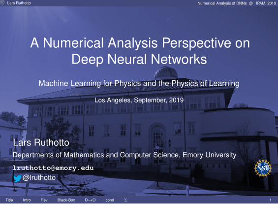
Agenda: Numerical Analysis of Deep Neural Networks
I Notation: Deep Learning
I Case 1: InvertibilityI Case 2: Time IntegratorsI Example: higher order or conservative?
I Case 3: Discretize-then-OptimizeI Example: Neural ODEs
I Case 4: Ill-conditioningI Example: Single layer neural network
I Conclusion and Summary
Key question: What can numerical analysts do in theage of ML?
Title Intro Rev Black-Box D→O cond Σ 2
Lars Ruthotto Numerical Analysis of DNNs @ IPAM, 2019
Deep Learning
Title Intro Rev Black-Box D→O cond Σ 3
Lars Ruthotto Numerical Analysis of DNNs @ IPAM, 2019
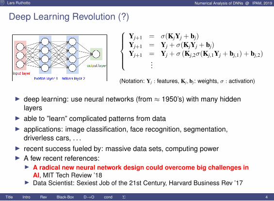
Deep Learning Revolution (?)Yj+1 = σ(KjYj + bj)Yj+1 = Yj + σ(KjYj + bj)Yj+1 = Yj + σ (Kj,2σ(Kj,1Yj + bj,1) + bj,2)
...
(Notation: Yj : features, Kj, bj: weights, σ : activation)
I deep learning: use neural networks (from ≈ 1950’s) with many hiddenlayers
I able to ”learn” complicated patterns from dataI applications: image classification, face recognition, segmentation,
driverless cars, . . .I recent success fueled by: massive data sets, computing powerI A few recent references:I A radical new neural network design could overcome big challenges in
AI, MIT Tech Review ’18I Data Scientist: Sexiest Job of the 21st Century, Harvard Business Rev ’17
Title Intro Rev Black-Box D→O cond Σ 4

Lars Ruthotto Numerical Analysis of DNNs @ IPAM, 2019
Optimal Control Framework for Deep Learning
training data, Y0,C prop. features, Y(T),C classification result
Supervised Deep Learning Problem
Given training data, Y0, and labels, C, find network parameters θ andclassification weights W, µ such that the DNN predicts the data-labelrelationship (and generalizes to new data), i.e., solve
minimizeθ,W,µ loss[g(W + µ),C] + regularizer[θ,W,µ]
Title Intro Rev Black-Box D→O cond Σ 5
Lars Ruthotto Numerical Analysis of DNNs @ IPAM, 2019
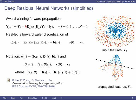
Deep Residual Neural Networks (simplified)
Award-winning forward propagation
Yj+1 = Yj + hKj,2σ(Kj,1Yj + bj), ∀ j = 0, 1, . . . ,N − 1.
ResNet is forward Euler discretization of
∂ty(t) = K2(t)σ (K1(t)y(t) + b(t)) , y(0) = y0.
Notation: θ(t) = (K1(t),K2(t),b(t)) and
∂ty(t) = f (y,θ(t)), y(0) = y0
where f (y,θ) = K2(t)σ (K1(t)y(t) + b(t)) .
K. He, X. Zhang, S. Ren, and J. SunDeep residual learning for image recognition.IEEE Conf. on CVPR, 770–778, 2016.
input features, Y0
propagated features, YN
Title Intro Rev Black-Box D→O cond Σ 6
Lars Ruthotto Numerical Analysis of DNNs @ IPAM, 2019
(Some) Related Work
DNNs as (stochastic) Dynamical SystemsI Weinan E, Proposal on ML via Dynamical
Systems, Commun. Math. Stat., 5(1), 2017.I E Haber, LR, Stable Architectures for DNNs,
Inverse Problems, 2017.I Q. Li, L. Chen, C. Tai, Weinan E, Maximum
Principle Based Algorithms, arXiv, 2017.I B. Wang, B. Yuan, Z. Shi, S. Osher, ResNets
Ensemble via the Feynman-Kac Formalism, arXiv,2018.
Numerical Time IntegratorsI Y. Lu, A. Zhong, Q. Li, B. Dong, Beyond Finite
Layer DNNs, arXiv, 2017.I B. Chang, L. Meng, E. Haber, LR, D. Begert, E.
Holtham, Reversible architectures for DNNs,AAAI, 2018.
I T. Chen, Y. Rubanova, J. Bettencourt, D.Duvenaud, Neural ODEs, NeurIPS, 2018.
I E. Haber, K. Lensink, E. Treister, LR, IMEXnet:Forward Stable DNN. ICML, 2019.
Optimal ControlI S. Gunther, LR, J.B. Schroder,
E.C. Cyr, N.R. Gauger,Layer-parallel training of ResNets,arXiv, 2018.
I A. Gholami, K. Keutzer, G. Biros,ANODE: Unconditionally AccurateMemory-Efficient Gradients forNeural ODEs, arXiv, 2019.
I T. Zhang, Z. Yao, A. Gholami, K.Keutzer, J. Gonzalez, G. Biros, M.Mahoney, ANODEV2: A CoupledNeural ODE Evolution Framework,arXiv, 2019.
PDE-motivated ApproachesI E. Haber, LR, E. Holtham,
Learning across scales - MultiscaleCNNs, AAAI, 2018.
I LR, E. Haber, DNNs motivated byPDEs, arXiv, 2018.
Title Intro Rev Black-Box D→O cond Σ 7
Lars Ruthotto Numerical Analysis of DNNs @ IPAM, 2019
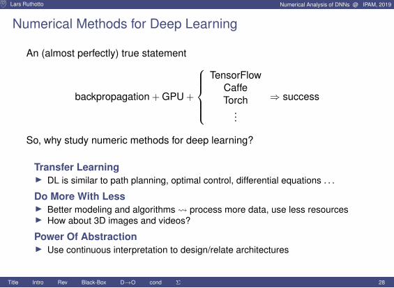
Numerical Methods for Deep Learning
An (almost perfectly) true statement
backpropagation + GPU +
TensorFlow
CaffeTorch
...
⇒ success
So, why study numeric methods for deep learning?
Title Intro Rev Black-Box D→O cond Σ 8
Lars Ruthotto Numerical Analysis of DNNs @ IPAM, 2019
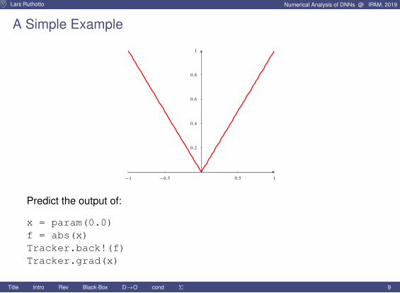
A Simple Example
−1 −0.5 0.5 1
0.2
0.4
0.6
0.8
1
Predict the output of:
x = param(0.0)f = abs(x)Tracker.back!(f)Tracker.grad(x)
Title Intro Rev Black-Box D→O cond Σ 9
Lars Ruthotto Numerical Analysis of DNNs @ IPAM, 2019
Case 1: Reversibility
Title Intro Rev Black-Box D→O cond Σ 10
Lars Ruthotto Numerical Analysis of DNNs @ IPAM, 2019
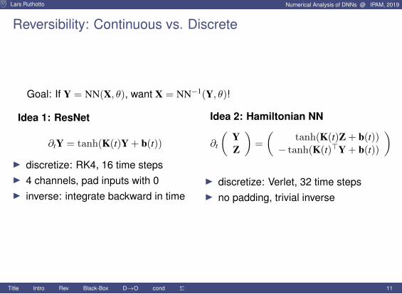
Reversibility: Continuous vs. Discrete
Goal: If Y = NN(X, θ), want X = NN−1(Y, θ)!
Idea 1: ResNet
∂tY = tanh(K(t)Y + b(t))
I discretize: RK4, 16 time stepsI 4 channels, pad inputs with 0I inverse: integrate backward in time
Idea 2: Hamiltonian NN
∂t
(YZ
)=
(tanh(K(t)Z + b(t))
− tanh(K(t)>Y + b(t))
)
I discretize: Verlet, 32 time stepsI no padding, trivial inverse
Title Intro Rev Black-Box D→O cond Σ 11
Lars Ruthotto Numerical Analysis of DNNs @ IPAM, 2019
Case 2: Black-box
Title Intro Rev Black-Box D→O cond Σ 12
Lars Ruthotto Numerical Analysis of DNNs @ IPAM, 2019
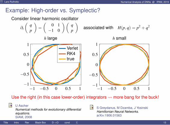
Example: High-order vs. Symplectic?Consider linear harmonic oscillator
∂t
(qp
)=
(0 1−1 0
)(qp
)associated with H(p, q) = p2 + q2
h large h small
−1 −0.5 0 0.5 1−1
−0.5
0
0.5
1VerletRK4true
−1 −0.5 0 0.5 1−1
−0.5
0
0.5
1
Use the right (in this case lower-order) integrators more bang for the buck!
U AscherNumerical methods for evolutionary differentialequations.SIAM, 2008
S Greydanus, M Dzamba, J YosinskiHamiltonian Neural Networks.arXiv:1906.01563
Title Intro Rev Black-Box D→O cond Σ 13
Lars Ruthotto Numerical Analysis of DNNs @ IPAM, 2019
Case 3: Discrete vs. Continuous
Title Intro Rev Black-Box D→O cond Σ 14
Lars Ruthotto Numerical Analysis of DNNs @ IPAM, 2019
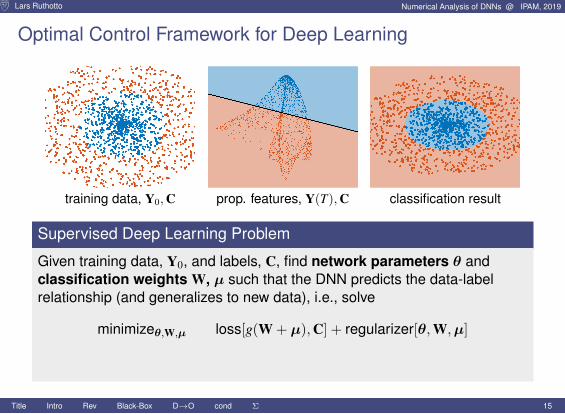
Optimal Control Framework for Deep Learning
training data, Y0,C prop. features, Y(T),C classification result
Supervised Deep Learning Problem
Given training data, Y0, and labels, C, find network parameters θ andclassification weights W, µ such that the DNN predicts the data-labelrelationship (and generalizes to new data), i.e., solve
minimizeθ,W,µ loss[g(W + µ),C] + regularizer[θ,W,µ]
Title Intro Rev Black-Box D→O cond Σ 15
Lars Ruthotto Numerical Analysis of DNNs @ IPAM, 2019
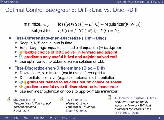
Optimal Control Background: Diff→Disc vs. Disc→Diff
minimizeθ,W,µ loss[g(WY(T) + µ),C] + regularizer[θ,W,µ]
subject to ∂tY(t) = f (Y(t),θ(t)) , Y(0) = Y0.
I First-Differentiate-then-Discretize ( Diff→Disc)I Keep θ,b,Y continuous in timeI Euler-Lagrange-Equations adjoint equation (≈ backprop)I flexible choice of ODE solver in forward and adjointI gradients only useful if fwd and adjoint solved wellI use optimization to obtain discrete solution of ELE
I First-Discretize-then-Differentiate (Disc→Diff)I Discretize θ,b,Y in time (could use different grids)I Differentiate objective (e.g., use automatic differentiation)I / gradients related to adjoints but no choice of solverI gradients useful even if discretization is inaccurateI use nonlinear optimization tools to approximate minimizer
MD GunzburgerPerspectives in flow controland optimization.SIAM, 2013.
TQ Chen et al.,Neural OrdinaryDifferential Equations.NeurIPS, 2018.
A Gholami, K Keutzer, G BirosANODE: UnconditionallyAccurate Memory-EfficientGradients for Neural ODEs.arXiv:1902.10298
Title Intro Rev Black-Box D→O cond Σ 16
Lars Ruthotto Numerical Analysis of DNNs @ IPAM, 2019
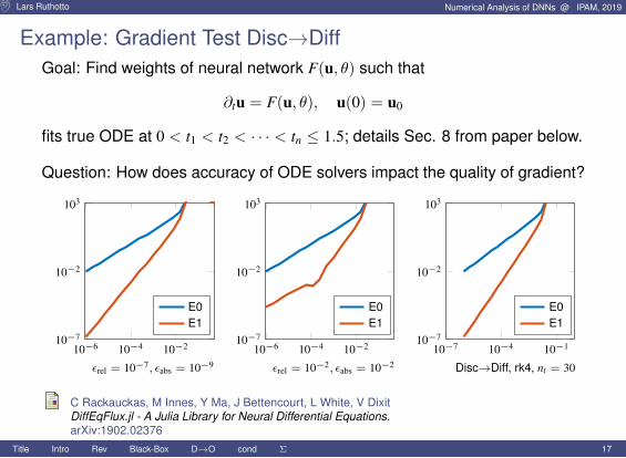
Example: Gradient Test Disc→DiffGoal: Find weights of neural network F(u, θ) such that
∂tu = F(u, θ), u(0) = u0
fits true ODE at 0 < t1 < t2 < · · · < tn ≤ 1.5; details Sec. 8 from paper below.
Question: How does accuracy of ODE solvers impact the quality of gradient?
10−6 10−4 10−210−7
10−2
103
E0E1
10−6 10−4 10−210−7
10−2
103
E0E1
10−7 10−4 10−110−7
10−2
103
E0E1
εrel = 10−7, εabs = 10−9 εrel = 10−2, εabs = 10−2 Disc→Diff, rk4, nt = 30
C Rackauckas, M Innes, Y Ma, J Bettencourt, L White, V DixitDiffEqFlux.jl - A Julia Library for Neural Differential Equations.arXiv:1902.02376
Title Intro Rev Black-Box D→O cond Σ 17
Lars Ruthotto Numerical Analysis of DNNs @ IPAM, 2019
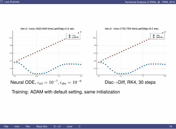
Neural ODE, εrel = 10−7, εabs = 10−9 Disc→Diff, RK4, 30 steps
Training: ADAM with default setting, same initialization
Title Intro Rev Black-Box D→O cond Σ 18
Lars Ruthotto Numerical Analysis of DNNs @ IPAM, 2019
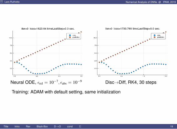
Neural ODE, εrel = 10−7, εabs = 10−9 Disc→Diff, RK4, 30 steps
Training: ADAM with default setting, same initialization
Title Intro Rev Black-Box D→O cond Σ 19
Lars Ruthotto Numerical Analysis of DNNs @ IPAM, 2019
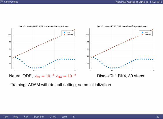
Neural ODE, εrel = 10−2, εabs = 10−2 Disc→Diff, RK4, 30 steps
Training: ADAM with default setting, same initialization
Title Intro Rev Black-Box D→O cond Σ 20
Lars Ruthotto Numerical Analysis of DNNs @ IPAM, 2019
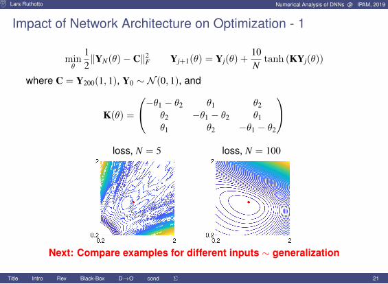
Impact of Network Architecture on Optimization - 1
minθ
12‖YN(θ)− C‖2
F Yj+1(θ) = Yj(θ) +10N
tanh (KYj(θ))
where C = Y200(1, 1), Y0 ∼ N (0, 1), and
K(θ) =
−θ1 − θ2 θ1 θ2θ2 −θ1 − θ2 θ1θ1 θ2 −θ1 − θ2
loss, N = 5 loss, N = 100
Next: Compare examples for different inputs ∼ generalization
Title Intro Rev Black-Box D→O cond Σ 21
Lars Ruthotto Numerical Analysis of DNNs @ IPAM, 2019
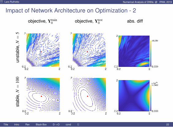
Impact of Network Architecture on Optimization - 2
objective, Ytrain0 objective, Ytest
0 abs. diffun
stab
le,N
=5
stab
le,N
=10
0
Title Intro Rev Black-Box D→O cond Σ 22
Lars Ruthotto Numerical Analysis of DNNs @ IPAM, 2019
Case 4: Conditioning
Title Intro Rev Black-Box D→O cond Σ 23
Lars Ruthotto Numerical Analysis of DNNs @ IPAM, 2019
Conditioning of the Learning ProblemConsider the regression problem with a single neural network layer
minW,K
12s‖R(W,K)‖2, where R(W,K) = Wσ(KY)− C
I Y ∈ Rd×s - input featuresI C ∈ Rn×s - output featuresI K ∈ Rm×d,W ∈ Rn×m - weights for fully-connected transformationI σ : R→ R - activation function (applied to each element)The problem above is a non-linear least squares problem (NNLS). Commonto look at the Jacobian of r, i.e., J = [JW JK] where
JW = σ(KY)> ⊗ I, and JK = (I⊗W) diag(σ′(KY)) (Y> ⊗ I)
(here, we vectorized R, I is identity, and ⊗ is the Kronecker product)
Q: What are the properties of J?
Title Intro Rev Black-Box D→O cond Σ 24

Lars Ruthotto Numerical Analysis of DNNs @ IPAM, 2019
Example: Condition Numbers
sing. vals. m = 8 sing. vals. m = 16 sing. vals. m = 32
0 10 20 3010−6
10−2
102
0 20 40 6010−6
10−2
102
0 20 40 60 80 10010−6
10−2
102
R(K,W) = Wσ(KY)− CI d = 3/n = 1 input/output featuresI s = 100 examples ∼ U([−1, 1]d)I m = {8, 16, 32} width of networkI σ = tanh
I K,W ∼ N (0, 1)
Discussion:I problem is ill-posed regularize!I cond(J) large smart LinAlgI how about single/half precision?I NNLS solvers will not be effectiveI need better initialization / method
Title Intro Rev Black-Box D→O cond Σ 25
Lars Ruthotto Numerical Analysis of DNNs @ IPAM, 2019
Conclusion
Title Intro Rev Black-Box D→O cond Σ 26
Lars Ruthotto Numerical Analysis of DNNs @ IPAM, 2019
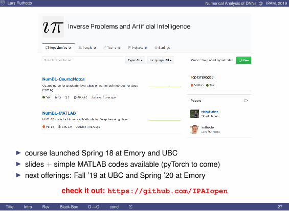
I course launched Spring 18 at Emory and UBCI slides + simple MATLAB codes available (pyTorch to come)I next offerings: Fall ’19 at UBC and Spring ’20 at Emory
check it out: https://github.com/IPAIopen
Title Intro Rev Black-Box D→O cond Σ 27
Lars Ruthotto Numerical Analysis of DNNs @ IPAM, 2019
Numerical Methods for Deep Learning
An (almost perfectly) true statement
backpropagation + GPU +
TensorFlow
CaffeTorch
...
⇒ success
So, why study numeric methods for deep learning?
Transfer LearningI DL is similar to path planning, optimal control, differential equations . . .
Do More With LessI Better modeling and algorithms process more data, use less resourcesI How about 3D images and videos?
Power Of AbstractionI Use continuous interpretation to design/relate architectures
Title Intro Rev Black-Box D→O cond Σ 28
Lars Ruthotto Numerical Analysis of DNNs @ IPAM, 2019
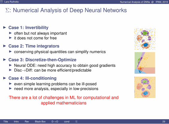
Σ: Numerical Analysis of Deep Neural Networks
I Case 1: InvertibilityI often but not always importantI it does not come for free
I Case 2: Time integratorsI conserving physical quantities can simplify numerics
I Case 3: Discretize-then-OptimizeI Neural ODE: need high accuracy to obtain good gradientsI Disc→Diff: can be more efficient/predictable
I Case 4: Ill-conditioningI even simple learning problems can be ill-posedI need more analysis, especially in low-precisions
There are a lot of challenges in ML for computational andapplied mathematicians
Title Intro Rev Black-Box D→O cond Σ 29