A new information-theoretic property about quantum states with anapplication to privacy in quantum communication∗

Rahul Jain† Jaikumar Radhakrishnan‡ Pranab Sen§

Abstract

We prove the following information-theoretic property about quantum states.

Substate theorem: Let ρ and σ be quantum states in the same Hilbert space with relativeentropy S(ρ‖σ) := Tr ρ(log ρ− log σ) = c. Then for all ε > 0, there is a state ρ′ such thatthe trace distance ‖ρ′ − ρ‖tr := Tr

√(ρ′ − ρ)2 ≤ ε, and ρ′/2O(c/ε2) ≤ σ.

It states that if the relative entropy of ρ and σ is small, then there is a state ρ′ close to ρ, i.e. with smalltrace distance ‖ρ′ − ρ‖tr, that when scaled down by a factor 2O(c) ‘sits inside’, or becomes a ‘substate’of, σ. This result has several applications in quantum communication complexity and cryptography.Using the substate theorem, we derive a privacy trade-off for the set membership problem in the two-party quantum communication model. Here Alice is given a subset A ⊆ [n], Bob an input i ∈ [n], andthey need to determine if i ∈ A.

Privacy trade-off for set membership: In any two-party quantum communication protocolfor the set membership problem, if Bob reveals only k bits of information about his input,then Alice must reveal at least n/2O(k) bits of information about her input.

We also discuss relationships between various information theoretic quantities that arise naturally in thecontext of the substate theorem.

1 Introduction

The main contribution of this paper is a theorem, called the substate theorem; it states, roughly, that if therelative entropy, S(ρ‖σ) := Tr ρ(log ρ − log σ), of two quantum states ρ and σ is at most c, then thereis a state ρ′ close to ρ such that ρ′/2O(c) sits inside σ. This implies that, as we will formalise later, stateσ can ‘masquerade’ as state ρ with probability 2−O(c) in many situations. Before we discuss the substatetheorem, let us first see a setting in which it is applied in order to get some motivation. This applicationconcerns the trade-off in privacy in two-party quantum communication protocols for the set membershipproblem [MNSW98]. After that, we discuss the substate theorem proper followed by a brief description ofseveral subsequent applications of the theorem.∗This paper is the journal version of several results that have previously appeared in the conference paper [JRS02].†Centre for Quantum Technologies and Department of Computer Science, National University of Singapore, Singapore,

rahul@comp.nus.edu.sg. Most of this work was done while the author was at Tata Institute of Fundamental Research, Mumbai,India, and partly at U.C. Berkeley, California, USA.‡School of Technology and Computer Science, Tata Institute of Fundamental Research, Mumbai, India, jaikumar@tifr.res.in.§School of Technology and Computer Science, Tata Institute of Fundamental Research, Mumbai, India, pgdsen@tcs.tifr.res.in.

Most of this work was done while the author was at Laboratoire de Recherche en Informatique, Universite de Paris–Sud, Orsay,France.

1

1.1 The set membership problem

Definition 1 In the set membership problem SetMembn, Alice is given a subsetA ⊆ [n] and Bob an elementi ∈ [n]. The two parties are required to exchange messages according to a fixed protocol in order for thelast recipient of a message to determine if i ∈ A. We often think of Alice’s input as a string x ∈ 0, 1nwhich we view as the characteristic vector of the setA; the protocol requires that in the end the last recipientoutput xi. In this viewpoint, Bob’s input i is called an index and the set membership problem is called theindex function problem.

The set membership problem is a fundamental problem in communication complexity. In the classicalsetting, it was studied by Miltersen, Nisan, Safra and Wigderson [MNSW98], who showed that if Bob sendsa total of at most b bits, then Alice must send n/2O(b) bits. Note that this is optimal up to constants, asthere is a trivial protocol where Bob sends the first b bits of his index to Alice, and Alice replies by sendingthe corresponding part of her bit string. The proof of Miltersen et al. relied on the richness technique theydeveloped to analyse such protocols. However, here is a simple round-elimination argument that gives thislower bound, and as we will see below, this argument generalises to the quantum setting. Fix a protocolwhere Bob sends a total of at most b bits, perhaps spread over several rounds. We can assume without lossof generality that Bob is the last recipient of a message, otherwise we can augment the protocol by makingAlice send the answer to Bob at the end which increases Alice’s communication cost by one bit. Modify thisprotocol as follows. In the new protocol, Alice and Bob use shared randomness to guess all the messagesof Bob. Alice sends her responses based on this guess. After this, if Bob finds that the guessed messagesare exactly what he wanted to send anyway, he accepts the answer given by the original protocol; otherwise,he aborts the protocol. Thus, if the original protocol was correct with probability p, the new one-roundprotocol, when it does not abort, which happens with probability at least 2−b, is correct with probability atleast p. A standard information theoretic argument now shows that in any such protocol Alice must send2−b · n(1−H(p)) bits (see e.g. [GKRdW06]; an argument as in [ANTV02] also gives a similar bound).

In the quantum setting, a special case of the set membership problem was studied by Ambainis, Nayak,Ta-Shma and Vazirani [ANTV02], where Bob is not allowed to send any message and there is no priorentanglement between Alice and Bob. They referred to this as quantum random access codes, because inthis setting the problem can be thought of as Alice encoding n classical bits x using qubits in such a waythat Bob is able to determine any one xi with probability at least p ≥ 1

2 . Note that in the quantum setting,unlike in its classical counterpart, it is conceivable that the measurement needed to determine xi makesthe state unsuitable for determining any of the other bits xj . In fact, Ambainis et al. exhibit a quantumrandom access code encoding two classical bits (x1, x2) into one qubit such that any single bit xi can berecovered with probability strictly greater than 1/2, which is impossible classically. Their main result,however, was that any such quantum code must have n(1 − H(p)) qubits (see also [Kla07, Theorem 5.8],for extension of this lower bound for entangled parties). They also gave a classical code with encodinglength n(1 − H(p)) + O(log n), thus showing that quantum random access codes provide no substantialimprovement over classical random access codes.

In this paper, we study the general set membership problem, where Alice and Bob are allowed to ex-change quantum messages over several rounds as well as share prior entanglement. Ashwin Nayak (privatecommunication) observed that the classical round elimination argument described above is applicable in thequantum setting: if Alice and Bob share prior entanglement in the form of EPR pairs, then using quan-tum teleportation [BBC+93], Bob’s messages can be assumed to be classical. Now, Alice can guess Bob’smessages, and we can combine the classical round elimination argument above with the results on randomaccess codes to show that Alice must send at least 2−(2b+1) · n(1−H(p)) qubits to Bob.

2

We strengthen these results and show that this trade-off between the communication required of Aliceand Bob is in fact a trade-off in their privacy: if a protocol has the property that Bob ‘leaks’ only a smallnumber of bits of information about his input, then in that protocol Alice must leak a large amount ofinformation about her input; in particular, she must send a large number of qubits. Before we present ourresult, let us explain what we mean when we say that Bob leaks only a small number of bits of informationabout his input. Fix a protocol for set membership. Assume that Bob’s input J is a random element of [n].Suppose Bob operates faithfully according to the protocol, but Alice deviates from it and manages to get herregisters, say A, entangled with J : we say that Bob leaks only b bits of information about his input if themutual information between J and A, I(J : A), is at most b. This must hold for all strategies adopted byAlice. Note that we do not assume that Bob’s messages contain only b qubits, they can be arbitrarily long. Inthe quantum setting, Alice has a big bag of tricks she can use in order to extract information from Bob. SeeSection 3.1 for an example of a cheating strategy for Alice, that exploits Alice’s ability to perform quantumoperations. We show the following result.

Result 1 (informal statement) If there is a quantum protocol for the set membership problem where Bobleaks only b bits of information about his input J , then Alice must leak Ω(n/2O(b)) bits of information abouther input x. In particular, this implies that Alice must send n/2O(b) qubits.

Related work: One can compare this with work on private information retrieval [CKGS98]. There, onerequires that the party holding the database x know nothing about the index i. Nayak [Nay99] sketched anargument showing that in both classical and quantum settings, the party holding the database has to sendΩ(n) bits/qubits to the party holding the index. Result 1 generalises Nayak’s argument and shows a trade-offbetween the loss in privacy for the database user Bob, and the loss in privacy for the database server Alice.

Recently, Klauck [Kla02] studied privacy in quantum protocols. In Klauck’s setting, two players col-laborate to compute a function, but at any point, one of the players might decide to terminate the protocoland try to infer something about the input of the other player using the bits in his possession. The playersare honest but curious: in a sense, they don’t deviate from the protocol in any way other than, perhaps, bystopping early. In this model, Klauck shows that there is a protocol for the set disjointness function whereneither player reveals more than O((log n)2) bits of information about his input, whereas in every classicalprotocol, at least one of the players leaks Ω(

√n/ log n) bits of information about his input. Our model

of privacy is more stringent. We allow malicious players who can deviate arbitrarily from the protocol.An immediate corollary of our result is that for the set membership problem, one of the players must leakΩ(log n) bits of information. This implies a similar loss in privacy for several other problems, including theset disjointness problem.

Privacy trade-off and the substate theorem: We now briefly motivate the need for the substate theoremin showing the privacy trade-off in Result 1 above. We know from the communication trade-off argumentfor set membership presented above that in any protocol for the problem, if Bob sends only b qubits, thenAlice must send n/2O(b) qubits. Unfortunately, this argument is not applicable when the protocol does notpromise that Bob sends only b qubits, but only ensures that the number of bits of information Bob leaks isat most b. So, the assumption is weaker. On the other hand, the conclusion now is stronger, for it assertsthat Alice must leak n/2O(b) bits of information, which implies that she must send at least these manyqubits. The above argument relied on the fact that Alice could generate a distribution on messages, so thatevery potential message of Bob is well-represented in this distribution: if Bob’s messages are classical andb bits long, the uniform distribution is such a distribution—each b bit message appears in it with probability2−b. Note that we are not assuming that messages of Bob have at most b qubits, so Alice cannot guess

3

these messages in this manner. Nevertheless, using only the assumption that Bob leaks at most b bits ofinformation about his input, the substate theorem provides us an alternative for the uniform distribution. Itallows us to prove the existence of a single quantum state that Alice and Bob can generate without access toBob’s input, after which if Bob is provided the input i, he can obtain the correct final state with probabilityat least 2−O(b) or abort if he cannot. After this, a standard quantum information theoretic argument impliesthat Alice must leak at least n/2O(b) bits of information about her input (see e.g. [GKRdW06]; an argumentas in [ANTV02] also gives a similar bound). The proof is discussed in detail in Section 3.

1.2 The substate theorem

It will be helpful to first consider the classical analogue of the substate theorem. Let P and Q be probabilitydistributions on the set [n] such that their relative entropy is bounded by c, that is

S(P‖Q) :=∑i∈[n]

P (i) log2

P (i)Q(i)

≤ c (1)

When c is small, this implies that P and Q are close to each other in total variation distance; indeed, onecan show that (see e.g. [CT91, Lemma 12.6.1])

‖P −Q‖1 :=∑i∈[n]

|P (i)−Q(i)| ≤√

(2 ln 2)c. (2)

That is, the probability of an event E ⊆ [n] in P is close to its probability in Q: |P (E) − Q(E)| ≤√(c ln 2)/2. Now consider the situation when c 1. In that case, expression (2) becomes weak, and it is

not hard to construct examples where ‖P −Q‖1 is very close to 2. Thus by bounding ‖P −Q‖1 alone, wecannot infer that an event E with probability 3/4 in P has any non-zero probability in Q. But is it true thatwhen S(P‖Q) < +∞ and P (E) > 0, then Q(E) > 0? Yes! To see this, let us reinterpret the expressionin (1) as the expectation of logP (i)/Q(i) as i is chosen according to P . Thus, one is lead to believe that ifS(P‖Q) ≤ c < +∞, then logP (i)/Q(i) is typically bounded by c, that is, P (i)/Q(i) is typically boundedby 2c. One can formalise this intuition and show, for all r ≥ 1,

Pri←P

[P (i)Q(i)

> 2r(c+1)

]<

1r. (3)

We now briefly sketch a proof of the above inequality. Note that since some terms involved in the relativeentropy expression (Eq. (1)) could be negative, we cannot apply the Markov’s inequality immediately. LetGood := i : P (i)/2r(c+1) ≤ Q(i), Bad := [n] \ Good. By concavity of the logarithm function, we get

P (Good) logP (Good)Q(Good)

+ P (Bad) logP (Bad)Q(Bad)

≤ S(P‖Q) ≤ c.

By elementary calculus, P (Good) log P (Good)Q(Good) > −1. Thus we get P (Bad) · r(c+ 1) < c+ 1, proving the

above inequality.We now define a new probability distribution P ′ as follows:

P ′(i) :=

P (i)

P (Good) i ∈ Good

0 i ∈ Bad,

that is, in P ′ we just discard the bad values of i and renormalise. Now, r−1r2r(c+1)P

′ is dominated by Qeverywhere. We have thus shown the classical analogue of the desired substate theorem.

4

Result 2’ (Classical substate theorem) Let P,Q be probability distributions on the same sample spacewith S(P‖Q) ≤ c. Then for all r > 1, there exist distributions P ′, P ′′ such that∥∥P − P ′∥∥

1≤ 2r

and Q = αP ′ + (1− α)P ′′,

where α := r−1r2r(c+1) .

Let us return to our event E that occurred with some small probability p in P . Now, if we take r tobe 2/p, then E occurs with probability at least p/2 in P ′, and hence appears with probability p/2O(c/p) inQ. Thus, we have shown that even though P and Q are far apart as distributions, events that have positiveprobability, no matter how small, in P , continue to have positive probability in Q.

The main contribution of this paper is a quantum analogue of Result 2’. To state it, we recall that therelative entropy of two quantum states ρ, σ in the same Hilbert space is defined as S(ρ‖σ) := Tr ρ(log ρ−log σ), and the trace distance between them is defined as ‖ρ− ρ′‖tr := Tr

√(ρ− ρ′)2.

Result 2 (Quantum substate theorem) Suppose ρ and σ are quantum states in the same Hilbert spacewith S(ρ‖σ) ≤ c. Then for all r > 1, there exist states ρ′, ρ′′ such that∥∥ρ− ρ′∥∥

tr≤ 2√

rand σ = αρ′ + (1− α)ρ′′,

where α := r−1r2rc′

and c′ := c+ 4√c+ 2 + 2 log(c+ 2) + 6.

The quantum substate theorem has been stated above in a form that brings out the analogy with the classicalstatement in Result 2’. In Section 4, we have a more nuanced statement which is often better suited forapplications.Remark: Using the quantum substate theorem and arguing as above, one can conclude that if an event Ehas probability p in ρ, then its probability q in σ is at least q ≥ p

2O(c/p2), c = S(ρ‖σ). Actually, one can

show the stronger result that q ≥ p2O(c/p) as follows. Using the fact that relative entropy cannot increase after

doing a measurement, we get

p logp

q+ (1− p) log

1− p1− q

≤ S(ρ‖σ) ≤ c.

We now argue as in the proof of Result 2’ to show the stronger lower bound on q.In view of this, one may wonder if there is any motivation at all in proving a quantum substate theorem.

Recall however, that the quantum substate theorem gives a structural relationship between ρ and σ whichis useful in many applications e.g. privacy trade-off for set membership discussed earlier. It does notseem possible in these applications to replace this structural relationship by considerations about the relativeprobabilities of an event E in ρ and σ. In our privacy trade-off application, σ plays the role of the statethat Alice and Bob can generate without access to Bob’s input, and ρ plays the role of the correct finalstate of Bob in the protocol. To prove the trade-off, σ should be able to ‘masquerade’ as ρ with probability2−O(b), b being the amount of information Bob leaks about his input. Also, Bob should know whether the‘masquerade’ succeeded or not so that he can abort if it fails, and it is this requirement that needs the substateproperty.

The ideas used to arrive at Result 2’ do not immediately generalise to prove Result 2, because ρ andσ need not be simultaneously diagonalisable. As it turns out, our proof of the quantum substate theoremtakes an indirect route. First, by exploiting the Fuchs and Caves [FC95] characterisation of fidelity and a

5

minimax theorem of game theory, we obtain a ‘lifting’ theorem about an ‘observational’ version of relativeentropy; this statement is interesting on its own. Using this ‘lifting’ theorem, and a connection between the‘observational’ version of relative entropy and actual relative entropy, we argue that it is enough to verifythe original statement when ρ and σ reside in a two-dimensional space and ρ is a pure state. The twodimensional case is then established by a direct computation.

1.3 Other applications of the substate theorem

The conference version of this paper [JRS02], in which the substate theorem was first announced, describedtwo applications of the theorem. The first application provided tight privacy trade-offs for the set mem-bership problem, which we have discussed above. This application is a good illustration of the use ofthe substate theorem, for several applications have the same structure. The second application showed tightlower bounds for the pointer chasing problem [NW93, KNTZ07], thereby establishing that the lower boundsshown by Ponzio, Radhakrishnan and Venkatesh [PRV01] in the classical setting are valid also for quantumprotocols without prior entanglement.

Subsequent to [JRS02], several applications of the classical and quantum substate theorems have beendiscovered. We briefly describe these results now. Earlier, in related but independent work Chakrabarti, Shi,Wirth and Yao [CSWY01] discovered their very influential information cost approach for obtaining directsum results in communication complexity. Jain, Radhakrishnan and Sen [JRS03] observed that the results ofChakrabarti et al. could be derived more systematically using the classical substate theorem. This approachallowed them to extend Chakrabarti et al.’s direct sum results, which applied to one-round and simultaneousmessage protocols under the uniform distribution on inputs, to two-party multiple round protocols under allproduct distributions on inputs. Ideas from [JRS03] were then applied by Chakrabarti and Regev [CR04]to obtain their tight lower bound on data structures for the approximate nearest neighbour problem on theHamming cube. The classical substate theorem has also been used by Jain, Klauck and Nayak [JKN08] inorder to prove direct product theorems for classical communication complexity.

The quantum substate theorem, the main result of this paper, has also found several other applications.Jain, Radhakrishnan and Sen [JRS05] used it to show how any two-party multiple round quantum protocolfor computing any relation, where Alice leaks only a bits of information about her input and Bob leaks onlyb bits of information about his, can be transformed to a one-round quantum protocol with prior entanglementwhere Alice transmits just a2O(b) bits to Bob. Note that plain Schumacher compression [Sch95] cannot beused to prove such a result, since we require a ‘one-shot’ as opposed to an asymptotic result. Also there canbe interaction in a general communication protocol, as well it could be that the reduced state of any singleparty can be mixed. Jain et al.’s compression result gives an alternative proof of Result 1, because the workof Ambainis et al. [ANTV02] implies that in any such protocol for set membership Alice must send Ω(n)bits to Bob. Jain et al. also used the classical and quantum substate theorems to prove worst case direct sumresults for simultaneous message and one round classical and quantum protocols, improving on [JRS03].More recently, using the quantum substate theorem Jain [Jai06] obtained a nearly tight characterisation ofthe communication complexity of remote state preparation, an area that has received considerable attentionlately. The substate theorem has also found application in the study of quantum cryptographic protocols:using it, Jain [Jai08] showed nearly tight bounds on the binding-concealing trade-offs for quantum stringcommitment schemes.

6

1.4 Organisation of the rest of the paper

In the next section, we recall some basic facts from classical and quantum information theory that willbe used in the rest of the paper. In Section 3, we formally define our model of privacy loss in quantumcommunication protocols and prove our privacy trade-off result for set membership assuming the substatetheorem. In Section 4, we give the actual statement of the substate theorem that is used in our privacy trade-offs, and a complete proof for it. Sections 3 and 4 may be read independently of each other. In Section 5we mention some open problems, and finally in the appendix we discuss relationships between variousinformation theoretic quantities that arise naturally in the context of the substate theorem. The appendixmay be read independently of Section 3.

2 Information theory background

We now recall some basic definitions and facts from classical and quantum information theory, which willbe useful later. For excellent introductions to classical and quantum information theory, see the books byCover and Thomas [CT91] and Nielsen and Chuang [NC00] respectively.

In this paper, all functions will have finite domains and ranges, all sample spaces will be finite, all ran-dom variables will have finite range and all Hilbert spaces are over complex numbers and finite dimensional.All logarithms are taken to base two. We will use the notationA ≥ B for operatorsA,B in the same Hilbertspace H as a shorthand for the statement ‘A − B is positive semidefinite’. Thus, A ≥ 0 denotes that Ais positive semidefinite and A > 0 denotes that A is (strictly) positive definite. For a positive semidefiniteoperator A,

√A denotes the unique positive semidefinite operator such that

√A ·√A = A.

We start off by recalling the definition of a quantum state.

Definition 2 (Quantum state) A quantum state or a density matrix in a Hilbert space H is a positivesemidefinite operator ρ onH with unit trace.

Note that a classical probability distribution can be thought of as a special case of a quantum state withdiagonal density matrix. An important class of quantum states are what are known as pure states, whichare states of the form |ψ〉〈ψ|, where |ψ〉 is a unit vector in H. Often, we abuse notation and refer to |ψ〉itself as the pure quantum state; note that this notation is ambiguous up to multiplication by a unit complexnumber. The support of a density matrix ρ, denoted by supp(ρ), is the span of eigenvectors correspondingto non-zero eigenvalues of ρ.

LetH,K be two Hilbert spaces and ω a quantum state in the bipartite systemH⊗K. The reduced quan-tum state ofH is given by tracing outK, also known as the partial trace TrK ω :=

∑k(11H⊗〈k|)ω(11H⊗|k〉)

where 11H is the identity operator on H and the summation is over an orthonormal basis for K. It is easy tosee that the partial trace is independent of the choice of the orthonormal basis for K. For a quantum state ρin H, any quantum state ω in H ⊗ K such that TrK ω = ρ is said to be an extension of ρ in H ⊗ K; if ω ispure, it is said, more specifically, to be a purification.

We next define a POVM element, which formalises the notion of a single outcome of a general measure-ment on a quantum state.

Definition 3 (POVM element) A POVM (positive operator valued measure) element F on Hilbert spaceH is a positive semidefinite operator onH such that F ≤ 11, where 11 is the identity operator onH.

We now define a POVM which represents the most general form of a measurement allowed by quantummechanics.

7

Definition 4 (POVM) A POVM F on Hilbert spaceH is a finite set of POVM elements F1, . . . , Fk onHsuch that

∑ki=1 Fi = 11, where 11 is the identity operator onH.

When a quantum state ρ ∈ H is measured according to the POVM Fi : i ∈ [k], the probability that out-come i ∈ [k] is observed is Tr (Fiρ). For a quantum state ρ in H, let Fρ denote the probability distributionp1, . . . , pk on [k], where pi := Tr (Fiρ).

Typically, the distance between two probability distributions P,Q on the same sample space Ω is mea-sured in terms of the total variation distance defined as ‖P −Q‖1 :=

∑i∈Ω |P (i) − Q(i)|. The quantum

analogue of the total variation distance is known as the trace distance.

Definition 5 (Trace distance) Let ρ, σ be quantum states in the same Hilbert space. Their trace distance isdefined as ‖ρ− σ‖tr := Tr

√(ρ− σ)2.

If we think of probability distributions as diagonal density matrices, then the trace distance between themis nothing but their total variation distance. For pure states |ψ〉, |φ〉 it is easy to see that their trace distanceis given by ‖|ψ〉〈ψ| − |φ〉〈φ|‖tr = 2

√1− |〈ψ|φ〉|2. The following fundamental fact shows that the trace

distance between two density matrices bounds how well one can distinguish between them by a POVM. Aproof can be found in [Hel76].

Fact 1 Let ρ, σ be density matrices in the same Hilbert space H. Let F be a POVM on H. Then,‖Fρ−Fσ‖1 ≤ ‖ρ− σ‖tr. Also, there is a two-outcome orthogonal measurement that achieves equal-ity above.

Another measure of distinguishability between two probability distributions P,Q on the same samplespace Ω is the Bhattacharya distinguishability coefficient defined as B(P,Q) :=

∑i∈Ω

√P (i)Q(i). Its

quantum analogue is known as fidelity. We will need several facts about fidelity in order to prove thequantum substate theorem.

Definition 6 (Fidelity) Let ρ, σ be density matrices in the same Hilbert space H. Their fidelity is definedas B(ρ, σ) := Tr

√√ρ σ√ρ.

The fidelity, or sometimes its square, is also referred to as the “transition probability” of Uhlmann. Forprobability distributions, the fidelity turns out to be the same as their Bhattacharya distinguishability coef-ficient. Jozsa [Joz94] gave an elementary proof for finite dimensional Hilbert spaces of the following basicand remarkable property about fidelity (also see [Uhl76]).

Fact 2 Let ρ, σ be density matrices in the same Hilbert space H. Then, B(ρ, σ) = supK,|ψ〉,|φ〉 |〈ψ|φ〉|,where K ranges over all Hilbert spaces and |ψ〉, |φ〉 range over all purifications of ρ, σ respectively inH⊗K. Also, for any Hilbert space K such that dim(K) ≥ dim(H), there exist purifications |ψ〉, |φ〉 of ρ, σinH⊗K, such that B(ρ, σ) = |〈ψ|φ〉|.

We will also need the following fact about fidelity, proved by Fuchs and Caves [FC95].

Fact 3 Let ρ, σ be density matrices in the same Hilbert spaceH. Then B(ρ, σ) = infF B(Fρ,Fσ), whereF ranges over POVMs onH. In fact, the infimum above can be attained by a complete orthogonal measure-ment onH.

The most general operation on a density matrix allowed by quantum mechanics is what is called acompletely positive trace preserving superoperator, or superoperator for short. Let H,K be Hilbert spaces.A superoperator T from H to K maps quantum states ρ in H to quantum states T ρ in K, and is described

8

by a finite collection of linear maps A1, . . . , Al from H to K called Kraus operators such that, T ρ =∑li=1AiρA

†i . Unitary transformations, taking partial traces and POVMs are special cases of superoperators.

LetX be a classical random variable. Let P denote the probability distribution induced byX on its rangeΩ. The Shannon entropy of X is defined as H(X) := H(P ) := −

∑i∈Ω P (i) logP (i). For any 0 ≤ p ≤ 1,

the binary entropy of p is defined asH(p) := H((p, 1−p)) = −p log p−(1−p) log(1−p). IfA is a quantumsystem with density matrix ρ, then its von Neumann entropy S(A) := S(ρ) := −Tr ρ log ρ. It is obvious thatthe von Neumann entropy of a probability distribution equals its Shannon entropy. If A,B are two disjointquantum systems, the mutual information of A and B is defined as I(A : B) := S(A) + S(B) − S(AB);mutual information of two random variables is defined analogously. By a quantum encodingM of a classicalrandom variable X on m qubits, we mean that there is a bipartite quantum system with joint density matrix∑

x Pr[X = x] · |x〉〈x|⊗ρx, where the first system is the random variable, the second system is the quantumencoding and an x in the range of X is encoded by a quantum state ρx on m qubits. The reduced state of thefirst system is nothing but the probability distribution

∑x Pr[X = x]·|x〉〈x| on the range ofX . The reduced

state of the second system is the average code word ρ :=∑

x Pr[X = x] · ρx. The mutual information ofthis encoding is given by I(X : M) = S(X) + S(M)− S(XM) = S(ρ)−

∑x Pr[X = x] · S(ρx).

We now define the relative entropy of a pair of quantum states.

Definition 7 (Relative entropy) If ρ, σ are quantum states in the same Hilbert space, their relative entropyis defined as S(ρ‖σ) := Tr (ρ(log ρ− log σ)).

For probability distributions P,Q on the same sample space Ω, the above definition reduces to S(P‖Q) =∑i∈Ω P (i) log P (i)

Q(i) . The following fact lists some useful properties of relative entropy. Proofs can be foundin [NC00, Chapter 11]. The monotonicity property below is also called Lindblad-Uhlmann monotonicity.

Fact 4 Let ρ, σ be density matrices in the same Hilbert spaceH. Then,

1. S(ρ‖σ) ≥ 0, with equality iff ρ = σ;

2. S(ρ‖σ) < +∞ iff supp(ρ) ⊆ supp(σ);

3. D(·‖·) is continuous in its two arguments over the domain of pairs of states (ρ, σ) such that supp(ρ) ⊆supp(σ);

4. (Unitary invariance) If U is a unitary transformation onH, S(UρU †‖UσU †) = S(ρ‖σ).

5. (Monotonicity) Let L be a Hilbert space and T be a completely positive trace preserving superoper-ator fromH to L. Then, S(T ρ‖T σ) ≤ S(ρ‖σ).

The following fact relates mutual information to relative entropy, and is easy to prove.

Fact 5 Let X be a classical random variable and M be a quantum encoding of X i.e. each x in the rangeof X is encoded by a quantum state ρx. Let ρ :=

∑x Pr[X = x] · ρx be the average code word. Then,

I(X : M) =∑

x Pr[X = x] · S(ρx‖ρ).

The next fact is an extension of the random access code arguments of [ANTV02], and was proved byGavinsky, Kempe, Regev and de Wolf [GKRdW06, Lemma 1].

Fact 6 Let X = X1 · · ·Xn be a classical random variable of n uniformly distributed bits. Let M be aquantum encoding of X on m qubits. For each i ∈ [n], suppose there is a POVM Fi on M with threeoutcomes 0, 1, ?. Let Yi denote the random variable obtained by applying Fi to M . Suppose there are real

9

numbers 0 ≤ λi, εi ≤ 1 such that Pr[Yi 6= ?] ≥ λi and Pr[Yi = Xi | Yi 6= ?] ≥ 1/2 + εi, where theprobability arises from the randomness in X as well as the randomness of the outcome of Fi. Then,

n∑i=1

λiε2i ≤

n∑i=1

λi(1−H(1/2 + εi)) ≤ I(X : M) ≤ m.

3 Privacy trade-offs for set membership

In this section, we prove a trade-off between privacy loss of Alice and privacy loss of Bob for the setmembership problem SetMembn assuming the substate theorem. We then embed index function into otherfunctions using the concept of VC-dimension and show privacy trade-offs for some other problems. Butfirst, we formally define our model of privacy loss in quantum communication protocols.

3.1 Quantum communication protocols

We consider two party quantum communication protocols as defined by Yao [Yao93]. Let X ,Y,Z be setsand f : X × Y → Z be a function. There are two players Alice and Bob, who hold qubits. Alice gets aninput x ∈ X and Bob an input y ∈ Y . When the communication protocol P starts, Alice and Bob each holdsome ‘work qubits’ initialised to the all-zeroes state. Alice and Bob may also share an input independentstate |ψ〉, providing ‘prior entanglement’. Thus, the initial superposition is simply |0〉|ψ〉|0〉, where the firstand last last registers denote the work qubits of Alice and Bob respectively. Some of the qubits of |ψ〉 belongto Alice, the rest belong to Bob. The players take turns to communicate to compute f(x, y). Suppose it isAlice’s turn. Alice makes a unitary transformation on the qubits in her possession depending on x only,and then send some qubits to Bob. Sending qubits does not change the overall superposition, but rather theownership of the qubits. This allows Bob to apply his next unitary transformation, which depends on y only,on his original qubits plus the newly received qubits. At the end of the protocol P , some qubits belongingto the last recipient, called the ‘answer qubits’, are measured in the computational basis so as to output ananswer P(x, y). For each (x, y) ∈ X × Y the unitary transformations that are applied, as well as the qubitsthat are to be sent in each round, the number of rounds, the choice of the starting player, and the designationof which qubits are to be treated as ‘answer qubits’ are specified in advance by the protocol P . We say thatP computes f with ε-error in the worst case, if maxx,y Pr[P(x, y) 6= f(x, y)] ≤ ε. We say that P computesf with ε-error with respect to a probability distribution µ on X ×Y , if E µ[Pr[P(x, y) 6= f(x, y)]] ≤ ε. Thecommunication complexity of P is defined to be the total number of qubits exchanged. Note that seeminglymore general models of communication protocols can be thought of where superoperators may be appliedby the parties instead of unitary transformations, and arbitrary POVM may be used in order to output theanswer of the protocol instead of measuring in the computational basis. But such models can be convertedto the unitary model above without changing the error probabilities, communication complexity, and as wewill see later, privacy loss to a cheating party.

Given a probability distribution µ on X × Y we define |µ〉 :=∑

(x,y)∈X×Y√µ(x, y) |x〉|y〉. Run-

ning protocol P with superposition |µ〉 fed to Alice’s and Bob’s inputs means that we first create the state∑(x,y)∈X×Y

√µ(x, y)|x〉|0〉|ψ〉|0〉|y〉, then feed the middle three registers to P and let P run its course.

We define the success probability of P when |µ〉 is fed to Alice’s and Bob’s inputs to be the probability thatmeasuring the inputs and the answer qubits in the computational basis at the end of P produces consistentresults. Running protocol P with mixture µ fed to Alice’s and Bob’s inputs means that we first create thestate

∑(x,y)∈X×Y µ(x, y)|x〉〈x||0〉〈0||ψ〉〈ψ||0〉〈0||y〉〈y|, then feed the middle three registers to P and let P

run its course. The success probability of P when mixture µ is fed to Alice’s and Bob’s inputs is defined

10

analogously. It is easy to see that the success probability of P on superposition |µ〉 is the same as the successprobability on mixture µ, and both are equal to Eµ[Pr[P(x, y) = f(x, y)]].

Now let µX , µY be probability distributions on X ,Y , and let µ := µX × µY denote the product distri-bution on X × Y . Let P be the prescribed honest protocol for f . In the ‘honest’ run of P mixture µ is fedto Alice’s and Bob’s inputs. Now let us suppose that Bob turns ‘malicious’ and deviates from the prescribedprotocol P in order to learn as much as he can about Alice’s input. Note that Alice remains honest in thisscenario i.e. she continues to follow P . Thus, Alice and Bob are now actually running a ‘cheating’ protocolP . Let registers A,X,B, Y denote Alice’s work qubits, Alice’s input qubits, Bob’s work qubits and Bob’sinput qubits respectively at the end of P . The privacy leakage from Alice to Bob in P is captured by themutual information IP(X : BY ) between Alice’s input register X and Bob’s registers BY at the end ofprotocol P . The notation IP(· : ·) is just used to emphasise the fact that we are referring to the standardmutual information between two quantum systems at the end of protocol P . Note that the state of registerXis still the mixture µX . We want to study how large sup IP(X : BY ) can be for a given function f , productdistribution µ, and protocol P , where the supremum is taken over all ‘cheating’ protocols P wherein Bobcan be arbitrarily malicious but Alice continues to follow P honestly. We shall call this quantity the privacyloss of P from Alice to Bob. Privacy leakage and privacy loss from Bob to Alice can be defined similarly.

One of the ways that Bob can cheat (even without Alice realising it!) is by running P with the super-position |µY〉 :=

∑y∈Y

√µY(y) |y〉 fed to register Y . Alice remains honest and follows P; the state of

her input register X continues to be the mixture µX . This method of cheating gives Bob at least as muchinformation about Alice’s input as in the ‘honest’ run of P when the mixture µY is fed to Y . Sometimes itcan give much more. Consider the set membership problem, where Alice has a bit string x which denotesthe characteristic vector of a subset of [n] and Bob has an i ∈ [n]. Consider a clean protocol P for the indexfunction problem. Recall that a protocol P is said to be clean if the work qubits of both the players exceptthe answer qubits are in the state |0〉 at the end of P . We shall show a privacy trade-off result for P underthe uniform distribution on the inputs of the two players. For simplicity, assume that P is errorless (an errorof 1/4 will only change the privacy losses by a multiplicative constant). Suppose Alice cheats by feedinga uniform superposition over bit strings into her input register X , and then running P . Bob is honest, andhas a random i ∈ [n]. At the end of this ‘cheating’ run of P , Alice applies a Hadamard transformation oneach of the registers Xj , 1 ≤ j ≤ n. Suppose she were to measure them now in the computational basis.For all j 6= i, she would measure |0〉 with probability 1. For j = i, she would measure 1 with probability1/2. Thus, Alice has extracted about log n/2 bits of information about Bob’s index i. An ‘honest’ run of Pwould have yielded Alice only 1 bit of information about i.

We now define a superpositional privacy loss inspired by the above example. We consider the ‘cheating’run ofP wherein mixture µX is fed to registerX and superposition |µY〉 to register Y . Denote this ‘cheating’run by P ′. Let I ′(X : BY ) denote the mutual information of Alice’s input register X with Bob’s registersBY at the end of protocol P ′. The notation I ′(· : ·) is just used to emphasise the fact that we are referringto the standard mutual information between two quantum systems at the end of protocol P ′.

Definition 8 (Superpositional privacy loss) The superpositional privacy loss of P for function f on theproduct distribution µ from Alice to Bob is defined as LP(f, µ,A,B) := I ′(X : BY ). The superpositionalprivacy loss from Bob to Alice, LP(f, µ,B,A), is defined similarly. The superpositional privacy loss of Pfor f , LP(f), is the maximum over all product distributions µ, of maxLP(f, µ,A,B), LP(f, µ,B,A).

Remarks:1. Our notion of superpositional privacy loss can be viewed as a quantum analogue of the “combinatorial-informational” bounded error measure of privacy loss, I∗c−i, in Bar-Yehuda et al. [BCKO93].

11

2. Klauck [Kla02], based on Cleve et al. [CvDNT98], has made a similar observation about Ω(n) privacyloss for clean protocols computing the inner product mod 2 function. The significance of our lower boundson privacy loss is that they make no assumptions about the protocol P .3. In the definition of privacy loss by Klauck [Kla02], a mixture according to distribution µ (not necessarilya product distribution) is fed to both Alice’s and Bob’s input registers. He does not consider the case ofsuperpositions being fed to input registers. For product distributions, our notion of privacy is more stringentthan Klauck’s, and in fact, the LP(f, µ,A,B) defined above is an upper bound (to within an additive factorof log |Z|) on Klauck’s privacy loss function.4. We restrict ourselves to product distributions because we allow Bob to cheat by putting a superpositionin his input register Y . He should be able to do this without any a priori knowledge of x, which impliesthat the distribution µ should be a product distribution. Also for defining privacy loss under non-productdistributions on inputs, the initial mutual information between the correlated inputs of the two parties mustbe taken into account.5. Consider a more general definition of privacy loss from Alice to Bob under a product distribution, whereAlice is honest but Bob can cheat in any fashion so long as the reduced state of Alice’s qubits after eachround is the same as in the honest protocol. This definition is trivially an upper bound on the superpositionalprivacy loss, so tradeoffs proved in the setting of superpositional privacy loss continue to hold in the moregeneral setting.

3.2 The privacy trade-off result

The theorem stated below is the formal version of Result 1 stated in the introduction.

Theorem 1 Consider a quantum protocol P for SetMembn where Alice is given a subset of [n] and Bob anelement of n. Let µ denote the uniform probability distribution on Alice’s and Bob’s inputs. Suppose P haserror at most 1/2− ε with respect to µ. Suppose LP(SetMembn, µ,B,A) ≤ k. Then,

LP(SetMembn, µ,A,B) ≥ n

2ε−3(14k+25)− 2.

Proof: Let registers A,X,B, Y denote Alice’s work qubits, Alice’s input qubits, Bob’s work qubits andBob’s input qubits respectively, at the end of protocol P . We can assume without loss of generalitythat the last round of communication in P is from Alice to Bob, since otherwise, we can add an extraround of communication at the end wherein Alice sends the answer qubit to Bob. This process increasesLP(SetMembn, µ,A,B) by at most two and does not increase LP(SetMembn, µ,B,A) (see e.g. the infor-mation theoretic arguments in [CvDNT98]). Thus at the end of P , Bob measures the answer qubit, which isa qubit in the register B, in the computational basis to determine f(x, y).

Let |ψi〉XAY B be the state vector of Alice’s and Bob’s qubits and (ρi)XA the density matrix of Alice’squbits at the end of the protocol P , when Alice is fed a uniform superposition over bit strings in her inputregister X and Bob is fed |i〉 in his input register Y . In this proof, the subscripts of pure and mixed statesdenote the registers which are in those states. Let 1/2 + εi be the success probability of P in this case.Without loss of generality, 0 ≤ εi ≤ 1/2. Consider a run, Run 1, of P where a uniform mixture ofindices is fed to register Y , and a uniform superposition over bit strings is fed to register X . Let 1/2 + εbe the success probability of P for Run 1, which is also the success probability of P with respect to µ.Then ε = (1/n)

∑ni=1 εi. Let I1(Y : AX) denote the mutual information of register Y with registers

AX at the end of Run 1 of P , where the subscript 1 emphasises the fact that we are considering Run 1 of

12

P . We know that I1(Y : AX) = LP(SetMembn, µ,B,A) ≤ k. Let ρXA := (1/n)∑n

i=1(ρi)XA andki := S((ρi)XA‖ρXA). Note that 0 ≤ ki <∞ by Fact 4. By Fact 5,

k ≥ I1(Y : AX) =1n

n∑i=1

S((ρi)XA‖ρXA) =1n

n∑i=1

ki.

Let k′i := ki + 4√ki + 2 + 2 log(ki + 2) + 6 and ri := (2/εi)2.

Let us now consider a run, Run 2, of P with uniform superpositions fed to registers X,Y . Let |φ〉XAY Bbe the state vector of Alice’s and Bob’s qubits at the end of Run 2 of P . Then, TrY B |φ〉〈φ| = ρXA, andthe success probability of P for Run 2 is 1/2 + ε. Let Q be an additional qubit. By the substate theorem(Theorem 2, Sec. 4.2 which is a nuanced version of Result 2), there exist states |ψ′i〉XAY BQ, |θ′i〉XAY BQsuch that ‖|ψi〉〈ψi| − |ψ′i〉〈ψ′i|‖tr ≤ 2/

√ri = εi and TrY BQ |φi〉〈φi| = ρXA where

|φi〉XAY BQ :=

√ri − 1ri2rik

′i

|ψ′i〉XAY B|1〉Q +

√1− ri − 1

ri2rik′i

|θ′i〉XAY B|0〉Q,

In fact, there exists a unitary transformation Ui on registers Y BQ, transforming the state |φ〉XAY B|0〉Q tothe state |φi〉XAY BQ.

For each i ∈ [n], let X ′i denote the classical random variable got by measuring the ith bit of register Xin state |φ〉XAY B . We now prove the following claim.

Claim 1 For each i ∈ [n], there is a POVMMi with three outcomes 0, 1, ? acting on Y B such that if Z ′i isthe result ofMi on |φ〉XAY B , then Pr[Z ′i 6= ?] ≥ 2−4ε−2

i (k′i+1), and Pr[Z ′i = X ′i | Z ′i 6= ?] ≥ 1/2 + εi/2.

Proof: The POVMMi proceeds by first bringing in the ancilla qubit Q initialised to |0〉Q, then applying Uito the registers Y BQ and finally measuring Q in the computational basis. If it observes |1〉Q,Mi measuresthe answer qubit in B in the computational basis and declares the result as Z ′i. If it observes |0〉Q, Mi

outputs ?.When applied to |φ〉XAY B ,Mi first generates |φi〉XAY BQ and then measures Q in the computational

basis. In the case whenMi measures |1〉 for qubit Q, which happens with probability

Pr[Z ′i 6= ?] =ri − 1ri2rik

′i

≥ 2−4ε−2i (k′i+1),

the state vector of XAY B collapses to |ψ′i〉. In this case by Fact 1,

Pr[Z ′i = X ′i|Z ′i 6= ?] ≥ 12

+ εi −12

∥∥|ψi〉〈ψi| − |ψ′i〉〈ψ′i|∥∥tr≥ 1

2+εi2.

Consider now a run, Run 3, of P when a uniform mixture over bit strings is fed to register X and auniform superposition over [n] is fed to register Y . Let ρXAY B denote the density matrix of the registersXAY B at the end of Run 3 of P . In fact, measuring in the computational basis the register X in the state|φ〉XAY B gives us ρXAY B; also, TrY B ρXAY B = ρXA. Let I3(X : Y B) denote the mutual informationbetween register X and registers Y B in the state ρXAY B , where the subscript 3 emphasises the fact that weare considering Run 3 of P . For each i ∈ [n], let Xi denote the classical random variable correspondingto the ith bit of register X in state ρXAY B . Then, X := X1 . . . Xn is a uniformly distributed bit string oflength n. Let Zi denote the result of POVMMi of the above claim applied to ρXAY B . Then sinceMi acts

13

only on the registers Y B, we get Pr[Zi 6= ?] = Pr[Z ′i 6= ?] ≥ 2−4ε−2i (k′i+1), and Pr[Zi = Xi | Zi 6= ?] =

Pr[Z ′i = X ′i | Zi 6= ?] ≥ 1/2 + εi/2. Define Good := i ∈ [n] : ki ≤ 2k/ε, εi ≥ ε/2. Since ∀i, ki ≥ 0and εi ≤ 1/2, by Markov’s inequality, |Good| > nε/2. By Fact 6,

I3(X : Y B) ≥n∑i=1

ε2i · 2−4ε−2i (k′i+1)

4≥

∑i∈Good

ε2i · 2−4ε−2i (k′i+1)

4

≥ nε3 · 2ε−3(2k+4√

2k+2+2 log(2k+2)+7)

32≥ n

2ε−3(2k+4√

2k+2+2 log(2k+2)+13)

≥ n

2ε−3(14k+25).

By the arguments in the first paragraph of this proof, we have LP(SetMembn, µ,A,B) ≥ I(X : Y B)− 2.This completes the proof of the theorem.

As we have mentioned earlier, this theorem has been generalised in [JRS05] in a suitable manner torelate the privacy loss for any relation in terms of its one-way communication complexity. We do not getinto the details of this statement here. Instead, we give a weaker corollary of the present theorem that relatesthe privacy loss of a function to the Vapnik-Chervonenkis dimension (VC-dimension) of its communicationmatrix.

Definition 9 (VC-dimension) For a boolean valued function f : X × Y → 0, 1, a set T ⊆ Y is X -shattered, if for all S ⊆ T there is an x ∈ X such that ∀y ∈ T : f(x, y) = 1⇔ y ∈ S. The VC-dimensionof f for X , VCX (f), is the largest size of such a X -shattered set T ⊆ Y . Similarly, the VC-dimension of ffor Y , VCY(f), is the largest size of a Y-shattered set T ⊆ X .

Informally, VCX (f) captures the size of the largest instance of the set membership problem SetMembnthat can be ‘embedded’ into f . Using this connection, one can trivially prove a privacy trade-off result forf in terms of VCX (f), VCY(f) by invoking Theorem 1. This generalises Klauck’s lower bound [Kla00]for the communication complexity of bounded error one-way quantum protocols for f in terms of its VC-dimension.

Corollary 1 Let f : X × Y → 0, 1 be a boolean valued function. Let VCX (f) = n. Then there is aproduct distribution µ on X × Y such that, if P is a quantum protocol for f with average error at most1/2− ε with respect to µ,

LP(f, µ,B,A) ≤ k ⇔ LP(f, µ,A,B) ≥ n

2ε−3(14k+25)− 2.

An analogous statement holds for VCY(f).

Proof: Since VCX (f) = n, there is a set T ⊆ Y , |T | = n which is shattered. Without loss of generality,T = [n]. For any subset S ⊆ T , there is an x ∈ X such that ∀y′ ∈ T : f(x, y′) = 1 ⇔ y′ ∈ S. We nowgive a reduction from SetMembn to f as follows: In SetMembn, Alice is given a subset S ⊆ [n] and Bob isgiven a y ∈ [n]. Alice and Bob run the protocol P for f on inputs x and y respectively, to solve SetMembn.The corollary now follows from Theorem 1.

The following consequence of Corr. 1 is immediate.

Corollary 2 Quantum protocols for set membership SetMembn, set disjointness for subsets of [n] and innerproduct modulo 2 in 0, 1n each suffer from Ω(log n) privacy loss.

Proof: Follows trivially from Corr. 1 since all the three functions have VC-dimension n.

14

4 The substate theorem

In this section, we prove the quantum substate theorem. But first, we state a fact from game theory that willbe used in its proof.

4.1 A minimax theorem

We will require the following minimax theorem from game theory, which is a consequence of the Kakutanifixed point theorem in real analysis.

Fact 7 Let A1, A2 be non-empty, convex and compact subsets of Rn for some n. Let u : A1 × A2 → R bea continuous function, such that

• ∀a2 ∈ A2, the set a1 ∈ A1 : ∀a′1 ∈ A1 u(a1, a2) ≥ u(a′1, a2) is convex; i.e. for every a2 ∈ A2, theset of points a1 ∈ A1, such that u(a1, a2) is maximum is a convex set. And

• ∀a1 ∈ A1, the set a2 ∈ A2 : ∀a′2 ∈ A2 u(a1, a2) ≤ u(a1, a′2) is convex, i.e. for every a1 ∈ A1, the

set of points a2 ∈ A2, such that u(a1, a2) is minimum is a convex set.

Then, there is an (a∗1, a∗2) ∈ A1 ×A2 such that

maxa1∈A1

mina2∈A2

u(a1, a2) = u(a∗1, a∗2) = min

a2∈A2

maxa1∈A1

u(a1, a2).

Remark: The above statement follows by combining Proposition 20.3 (which shows the existence of Nashequilibrium a∗ in strategic games) and Proposition 22.2 (which connects Nash equilibrium and the min-maxtheorem for games defined using a pay-off function such as u) of Osborne and Rubinstein’s [OR94, pages19–22] book on game theory.

4.2 Proof of the substate theorem

We now state the quantum substate theorem as it is actually used in our privacy lower bound proofs.

Theorem 2 (Quantum substate theorem) Consider two Hilbert spaces H and K, dim(K) ≥ dim(H).Let C2 denote the two dimensional complex Hilbert space. Let ρ, σ be density matrices in H. Let r > 1be any real number. Let k := S(ρ‖σ). Let |ψ〉 be a purification of ρ in H ⊗ K. Then there exist purestates |φ〉, |θ〉 ∈ H ⊗ K and |ζ〉 ∈ H ⊗ K ⊗ C2, depending on r, such that |ζ〉 is a purification of σ and‖|ψ〉〈ψ| − |φ〉〈φ|‖tr ≤ 2/

√r, where

|ζ〉 :=

√r − 1r2rk′

|φ〉|1〉+

√1− r − 1

r2rk′|θ〉|0〉 and k′ := k + 4

√k + 2 + 2 log(k + 2) + 6.

Remarks:1. Note that Result 2 in the introduction follows from above by tracing out K ⊗ C2.2. From Result 2, one can easily see that ‖ρ− σ‖tr ≤ 2 − 2−O(k). This implies a 2−O(k) lower bound onthe fidelity of ρ and σ.

Overview of the proof of Theorem 2: As we have mentioned earlier, our proof of the quantum substatetheorem goes through by first defining a new notion of distinguishability called observational divergence,D(ρ‖σ), between two density matrices ρ, σ in the same Hilbert space H. Informally speaking, this notion

15

is a single observational version of relative entropy. Truly speaking, the substate theorem is a relationshipbetween observational divergence and the substate condition. The main steps of our proof of the substatetheorem are as follows:

1. We first prove an observational divergence ’lifting’ theorem, Theorem 3, which shows that given twostates ρ, σ in H and any extension σ′ of σ in H⊗K, dim(K) ≥ dim(H), one can find a purification|φ〉 of ρ inH⊗K such that D(|φ〉〈φ|‖σ′) = O(D(ρ‖σ)). This result may be of independent interest.

2. Theorem 3 is in turn shown using Lemmas 1, 2. Lemma 1 can be thought of as an ‘observational’substate result, i.e., a substate result with respect to a fixed POVM element, say F . We then proveLemma 2 which, for any fixed 0 ≤ p ≤ 1, removes the dependence on F if F satisfies Tr (F |ψ〉〈ψ|) ≥p. The dependence on parameter p is finally removed by performing a ‘discrete integration’ operation,giving us Theorem 3.

3. Theorem 3 helps us reduce the final statement we intend to prove (Theorem 2) to the case when ρis a pure state. The substate theorem when ρ is a pure state is shown in Lemma 3. In the proof ofLemma 3, we further reduce this case to analysing only a two dimensional scenario which is thenresolved by a direct calculation.

4. Finally Theorem 2, that is, the quantum substate theorem for relative entropy is established by usingProposition 2 which shows that observational divergence is never much bigger than relative entropyfor any pair of states.

Let us begin by defining observational divergence.

Definition 10 (Observational divergence) Let ρ, σ be density matrices in the same Hilbert spaceH. Theirobservational divergence is defined as

D(ρ‖σ) := supF

(Tr (Fρ) log

Tr (Fρ)Tr (Fσ)

),

where F above ranges over POVM elements onH such that Tr (Fσ) 6= 0.

The following properties of observational divergence follow easily from the definition.

Proposition 1 Let ρ, σ be density matrices in the same Hilbert spaceH. Then

1. D(ρ‖σ) ≥ 0, with equality iff ρ = σ.

2. D(ρ‖σ) < +∞ iff supp(ρ) ⊆ supp(σ). If D(ρ‖σ) < +∞, then there is a POVM element F whichachieves equality in Definition 10.

3. D(·‖·) is continuous in its two arguments over the domain of pairs of states (ρ, σ) such that supp(ρ) ⊆supp(σ);

4. (Unitary invariance) If U is a unitary transformation onH, D(UρU †‖UσU †) = D(ρ‖σ).

5. (Monotonicity) Suppose K is a Hilbert space, and ρ′, σ′ are extensions of ρ, σ in H ⊗ K. Then,D(ρ′‖σ′) ≥ D(ρ‖σ). This implies, via unitary invariance and the Kraus representation theorem,that if T is a completely positive trace preserving superoperator from H to a Hilbert space L, thenD(T ρ‖T σ) ≤ D(ρ‖σ).

16

Fact 4 and Proposition 1 seem to suggest that relative entropy and observational divergence are similarquantities. In fact, the relative entropy is an upper bound on the observational divergence to within anadditive constant. More properties of observational divergence as well as comparisons with relative entropyare discussed in the appendix.

Proposition 2 Let ρ, σ be density matrices in the same Hilbert spaceH. Then, D(ρ‖σ) < S(ρ‖σ) + 1.

Proof: By Fact 4 and Proposition 1, D(ρ‖σ) = +∞ iff supp(ρ) 6⊆ supp(σ) iff S(ρ‖σ) = +∞. Thus, wecan henceforth assume without loss of generality that D(ρ‖σ) < +∞. By Proposition 1, there is a POVMelement F such that D(ρ‖σ) = p log(p/q), where p := Tr (Fρ) and q := Tr (Fσ). We now have

S(ρ‖σ) ≥ p logp

q+ (1− p) log

(1− p)(1− q)

> p logp

q+ (1− p) log

1(1− q)

− 1 ≥ p logp

q− 1

= D(ρ‖σ)− 1.

The first inequality follows from the Lindblad-Uhlmann monotonicity of relative entropy (Fact 4), and thesecond inequality follows because (1− p) log(1− p) ≥ (− log e)/e > −1, for 0 ≤ p ≤ 1. This completesthe proof of the lemma.

We next prove the ‘observational’ substate lemma for a fixed POVM element, as mentioned before inthe overview.

Lemma 1 Consider two Hilbert spaces H and K, dim(K) ≥ dim(H). Let ρ, σ be density matrices in H.Let |ψ〉 be a purification of ρ inH⊗K. Let F be a POVM element onH⊗K. Let β > 1. Then there existsa purification |φ〉 of σ in H ⊗ K such that q ≥ p

2k′/p , where p := Tr (F |ψ〉〈ψ|), q := Tr (F |φ〉〈φ|) and

k′ := βD(ρ‖σ)− 2 log(1− β−1/2).

Proof: We assume without loss of generality that 0 < D(ρ‖σ) < +∞ and that p > 0. Let n := dim(H⊗K)and |αi〉ni=1 be the orthonormal eigenvectors of F with corresponding eigenvalues λini=1. Note that0 ≤ λi ≤ 1 and |αi〉 ∈ H ⊗K. We have from definition of p,

p =n∑i=1

λi|〈αi|ψ〉|2. (4)

Define,

|θ′〉 :=∑n

i=1 λi〈αi|ψ〉|αi〉√p

and |θ〉 :=|θ′〉‖|θ′〉‖

. (5)

Note that p = |〈ψ|θ〉|2‖|θ′〉‖2 and 0 < ‖|θ′〉‖2 ≤ 1. We will show later that there exists a purification |φ〉 ofσ inH⊗K such that

|〈φ|θ〉|2 ≥ |〈ψ|θ〉|2

2k′/|〈ψ|θ〉|2. (6)

17

This would imply,

p

2k′/p=

|〈ψ|θ〉|2‖|θ′〉‖2

2k′/(|〈ψ|θ〉|2‖|θ′〉‖2)≤ |〈ψ|θ〉|

2‖|θ′〉‖2

2k′/|〈ψ|θ〉|2(since 0 < ‖|θ′〉‖2 ≤ 1)

≤ |〈φ|θ〉|2‖|θ′〉‖2 (from Eq. (6))

= |〈φ|θ′〉|2 =|∑n

i=1 λi〈αi|ψ〉〈φ|αi〉|2

p(from Eq. (5))

=|∑n

i=1 λi〈αi|ψ〉〈φ|αi〉|2∑n

i=1 λi|〈αi|ψ〉|2(from Eq. (4))

≤n∑i=1

λi|〈αi|φ〉|2 (from the Cauchy-Schwarz inequality)

= Tr (F |φ〉〈φ|),

and we would be done.For getting the desired |φ〉 as Eq. (6), let us first define the density matrix τ inH as τ := TrK |θ〉〈θ|. By

Facts 2 and 3, there is a purification |φ〉 of σ inH⊗K and a POVM F1, . . . , Fl inH such that,

|〈φ|θ〉| = B(τ, σ) =l∑

i=1

√cibi,

where ci := Tr (Fiτ) and bi := Tr (Fiσ). Let ai := Tr (Fiρ). We know from Facts 2 and 3 that

0 <√p ≤ |〈ψ|θ〉| ≤ B(τ, ρ) ≤

l∑i=1

√ciai.

Note that the ai’s are non-negative real numbers summing up to 1, and so are the bi’s and the ci’s.For β > 1, define the set Sβ :=

i ∈ [l] : ai > bi · 2βk/B(τ,ρ)2

, where k := D(ρ‖σ). Note that

∀i ∈ S, bi 6= 0 as supp(ρ) ⊆ supp(σ), k being finite. Define the POVM elementG onH asG :=∑

i∈Sβ Fi.

Let a := Tr (Gρ) and b := Tr (Gσ). Then a =∑

i∈Sβ ai, b =∑

i∈Sβ bi, b > 0 and a > b · 2βk/B(τ,ρ)2 . Wehave that

D(ρ‖σ) = k ≥ a loga

b>

βka

B(τ, ρ)2⇒ a <

B(τ, ρ)2

β.

Now, by the Cauchy-Schwarz inequality and the other inequalities proved above, we get

B(τ, ρ) ≤l∑

i=1

√ciai =

∑i∈Sβ

√ciai +

∑i 6∈Sβ

√ciai

≤√∑i∈Sβ

ci

√∑i∈Sβ

ai + 2βk/(2B(τ,ρ)2)∑i 6∈Sβ

√cibi ≤ 1 ·

√a+ 2βk/(2B(τ,ρ)2)B(τ, σ)

<B(τ, ρ)√

β+ 2βk/(2B(τ,ρ)2)B(τ, σ).

This shows that

B(τ, ρ)2 < (1− β−1/2)−2 · 2βk/B(τ,ρ)2B(τ, σ)2 ⇒ |〈ψ|θ〉|2 < (1− β−1/2)−2 · 2βk/|〈ψ|θ〉|2 |〈φ|θ〉|2.

18

Since k′ = βk − 2 log(1− β−1/2), we get |〈φ|θ〉|2 ≥ |〈ψ|θ〉|2

2k′/|〈ψ|θ〉|2 , completing the proof of the lemma.

In the previous lemma, the purification |φ〉 of σ was a function of the POVM element F . We now provea lemma which, for any fixed 0 ≤ p ≤ 1, removes the dependence on F satisfying Tr (F |ψ〉〈ψ|) ≥ p, at theexpense of having a, in general, mixed extension of σ in the place of a pure extension i.e. purification.

Lemma 2 Consider two Hilbert spaces H and K, dim(K) ≥ dim(H). Let ρ, σ be density matrices in Hand |ψ〉 be a purification of ρ in H ⊗ K. Let 0 ≤ p ≤ 1 and β > 1. Then there exists an extension ω of σin H ⊗ K such that for all POVM elements F on H ⊗ K such that Tr (F |ψ〉〈ψ|) ≥ p, Tr (Fω) ≥ p/2k

′/p,where k′ := βD(ρ‖σ)− 2 log(1− β−1/2).

Proof: We assume without loss of generality that 0 < D(ρ‖σ) < +∞ and that p > 0. Consider theset A1 of all extensions ω of σ in H ⊗ K and the set A2 of all POVM operators F in H ⊗ K such thatTr (F |ψ〉〈ψ|) ≥ p. Observe that A1, A2 are non-empty, compact, convex sets. Without loss of generality,A2 is non-empty. Thus from Lemma 1, for every F ∈ A2, we have a purification |φF 〉 ∈ H ⊗ K of σ suchthat

Tr(F |φF 〉〈φF |

)≥ Tr (F |ψ〉〈ψ|)

2k′/Tr (F |ψ〉〈ψ|)≥ p

2k′/p.

Let us define u : A1 × A2 → R as ∀ω ∈ A1, ∀F ∈ A2, u(ω, F ) = Tr Fω. Note that with these definitions,the conditions of Fact 7 are trivially satisfied (note that we think of our matrices, which in general havecomplex entries, as vectors in a larger real vector space). Therefore, using Fact 7, we see that there exists anextension ω of σ inH⊗K such that Tr (Fω) ≥ p

2k′/p for all F ∈ A1. This completes the proof.

The previous lemma depends upon the parameter p. We now remove this restriction by performing a‘discrete integration’ operation and obtain the ’observational divergence lifting’ result. This result relatesthe observational divergence of a pair of density matrices to the observational divergence of their extensionsin an extended Hilbert space, where the extension of the first density matrix is a pure state. This may be ofindependent interest.

Theorem 3 (Observational divergence lifting) Consider two Hilbert spaces H,K, dim(K) ≥ dim(H).Let ρ, σ be density matrices inH, and |ψ〉 be a purification of ρ inH⊗K. Then there exists an extension ωof σ inH⊗K such that D((|ψ〉〈ψ|) ‖ω) < D(ρ‖σ) + 4

√D(ρ‖σ) + 1 + 2 log(D(ρ‖σ) + 1) + 5.

Proof: We assume without loss of generality that 0 < D(ρ‖σ) < +∞. Let β > 1 and γ ≥ 1. Define themonotonically increasing function f : [0, 1]→ [0, 1] as follows:

f(p) :=p

2k′/pwhere 0 ≤ p ≤ 1 and k′ := βD(ρ‖σ)− 2 log(1− β−1/2).

For a fixed positive integer l, define Tγ(l) :=∑l

i=1 lγ−1. It is easy to see by elementary calculus that

γ−1 ·lγ ≤ Tγ(l) ≤ γ−1 ·(l+1)γ .Define the density matrix ωl inH⊗K as ωl := (Tγ(l))−1∑l

i=1 iγ−1ω(i/l),

where for 0 ≤ p ≤ 1, ω(p) is an extension of σ in H ⊗ K such that Tr (Fω(p)) ≥ f(p) for all POVMelements F on H ⊗ K satisfying Tr (F |ψ〉〈ψ|) ≥ p. Such an ω(p) exists by Lemma 2. Then, TrK ωl = σi.e. ωl is an extension of σ inH⊗K.

Suppose F is a POVM element on H ⊗ K. Define p := Tr (F |ψ〉〈ψ|). Choose an integer l satisfyingl ≥ 1/p. Let j/l ≤ p < (j + 1)/l, where j is an integer satisfying 1 ≤ j ≤ l. We assume without loss of

19

generality that p > 0. Then,

Tr (Fωl) =1

Tγ(l)

j∑i=1

iγ−1 · Tr (Fω(i/l))

≥ 1Tγ(l)

j∑i=1

iγ−1 · f(i/l)

≥ Tγ(j)Tγ(l)

· f

(1

Tγ(j)

j∑i=1

iγ

l

)=

Tγ(j)Tγ(l)

· f(Tγ+1(j)l · Tγ(j)

)≥

(j

l + 1

)γ· f(

γ · jγ+1

l(γ + 1) · (j + 1)γ

)≥

(pl − 1l + 1

)γ· f((

γ(pl − 1)(γ + 1)l

)(pl − 1pl + 1

)γ).

The second inequality above follows from the convexity of f(·). By compactness, the set ωl : l ∈ N haslimit points. Choose a limit point point ω. By standard continuity arguments, TrK ω = σ and

q := Tr (Fω) ≥ liml→+∞

[(pl − 1l + 1

)γ· f((

γ(pl − 1)(γ + 1)l

)(pl − 1pl + 1

)γ)]= pγ · f

(γp

γ + 1

)=

γ · pγ+1

(γ + 1) · 2k′(γ+1)γ−1p−1 .

Hence, q > 0 and

p logp

q≤ p log

(γ−1(γ + 1) · p−γ · 2k′(γ+1)γ−1p−1

)= p log(1 + γ−1)− γp log p+ (1 + γ−1)k′

< (1 + γ−1)k′ + γ + 1.

The second inequality follows because −p log p < 1 for 0 ≤ p ≤ 1, and log(1 + γ−1) ≤ 1 for all γ ≥ 1.Substituting k′ = βD(ρ‖σ)− 2 log(1− β−1/2) gives

D((|ψ〉〈ψ|) ‖ω) < β(1 + γ−1)D(ρ‖σ)− 2(1 + γ−1) log(1− β−1/2) + γ + 1.

We set β = (1 + (D(ρ‖σ) + 1)−1/2)2 and γ = (D(ρ‖σ) + 1)1/2 to get

D((|ψ〉〈ψ|) ‖ω) < (1 + (D(ρ‖σ) + 1)−1/2)3 ·D(ρ‖σ) + (D(ρ‖σ) + 1)1/2 + 1

− 2(1 + (D(ρ‖σ) + 1)−1/2) · log(D(ρ‖σ) + 1)−1/2

1 + (D(ρ‖σ) + 1)−1/2

< (1 + (D(ρ‖σ) + 1)−1/2)3 ·D(ρ‖σ) + (D(ρ‖σ) + 1)1/2 + 1+ (1 + (D(ρ‖σ) + 1)−1/2) · log(D(ρ‖σ) + 1)

< D(ρ‖σ) + 4√D(ρ‖σ) + 1 + (1 + (D(ρ‖σ) + 1)−1/2) · log(D(ρ‖σ) + 1) + 5

< D(ρ‖σ) + 4√D(ρ‖σ) + 1 + 2 log(D(ρ‖σ) + 1) + 5.

This completes the proof of the lemma.We now prove the following lemma, which can be thought of as a substate result when the first density

matrix is in fact a pure state.

20

Lemma 3 Let |ψ〉 be a pure state and σ be a density matrix in the same Hilbert space H. Let k :=D ((|ψ〉〈ψ|)‖σ). Then for all r ≥ 1, there exists a pure state |φ〉, depending on r, such that

‖|ψ〉〈ψ| − |φ〉〈φ|‖tr <2√r

and(r − 1r2rk

)|φ〉〈φ| < σ.

Proof: We assume without loss of generality that 0 < k < +∞. Consider M := σ − (|ψ〉〈ψ|/2rk).We claim that M has at most one negative eigenvalue. This is because, from Weyl’s inequality [Bha97,Theorem III.2.1], no eigenvalue of a matrix decreases on adding a positive semi-definite matrix. Since σ ispositive semi-definite, adding it to −(|ψ〉〈ψ|/2rk) to produce M , cannot decrease any eigenvalue. Hence atmost one eigenvalue of M can be negative, since −(|ψ〉〈ψ|/2rk) has exactly one negative eigenvalue viz.−1/2rk, and the rest are zero.

If M ≥ 0 we take |φ〉 to be |ψ〉. The lemma trivially holds in this case.Otherwise, let |w〉 be the eigenvector corresponding to the unique negative eigenvalue−α ofM . Think-

ing of |w〉〈w| as a POVM element, we get

0 > −α = Tr (M |w〉〈w|) = 〈w|σ|w〉 − |〈ψ|w〉|2

2rk⇒ 〈w|σ|w〉 < |〈ψ|w〉|

2

2rk.

Hence

k = D(|ψ〉〈ψ|‖σ) ≥ |〈ψ|w〉|2 log|〈ψ|w〉|2

〈w|σ|w〉> rk|〈ψ|w〉|2 ⇒ |〈ψ|w〉|2 < 1

r≤ 1.

In particular, this shows that |ψ〉, |w〉 are linearly independent.Let n := dim(H). Let |v〉, |w〉 be an orthonormal basis for the two dimensional subspace of H

spanned by |ψ〉, |w〉. Extend it to |v1〉, . . . , |vn−2〉, |v〉, |w〉, an orthonormal basis for the entire spaceH. In this basis we have the following matrix equation,

F e d

e† a bd† b† c

−

0 0 0

0† x y0† y† z

=

P l

l† −α

, (7)

where the first, second and third matrices are σ, |ψ〉〈ψ|/2rk and M respectively. F is an (n− 2)× (n− 2)matrix, P is an (n − 1) × (n − 1) matrix, d, e are (n − 2) × 1 matrices and l is an (n − 1) × 1 matrix.a, c, x, z, α are non-negative real numbers and b, y are complex numbers. The zeroes above denote all zeromatrices of appropriate dimensions. The dagger denotes conjugate transpose.

Claim 2 We have the following properties.

1. b, y ∈ C, a, c, x, z, α ∈ R.

2. b = y 6= 0, 1/(r2rk) > z = c+α > c > 0, α > 0, a > 0, 0 < x < 1/2rk, x+ z = 1/2rk, l = 0 andd = 0.

3. 0 < xc|b|2 <

xz|y|2 = 1.

21

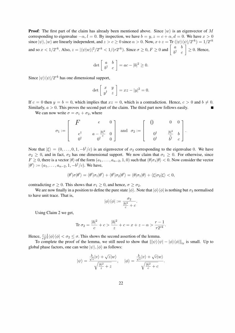
Proof: The first part of the claim has already been mentioned above. Since |w〉 is an eigenvector of Mcorresponding to eigenvalue −α, l = 0. By inspection, we have b = y, z = c + α, d = 0. We have x > 0since |ψ〉, |w〉 are linearly independent, and z > c ≥ 0 since α > 0. Now, x+z = Tr (|ψ〉〈ψ|/2rk) = 1/2rk

and so x < 1/2rk. Also, z = |〈ψ|w〉|2/2rk < 1/(r2rk). Since σ ≥ 0, F ≥ 0 and[a bb† c

]≥ 0. Hence,

det[a bb† c

]= ac− |b|2 ≥ 0.

Since |ψ〉〈ψ|/2rk has one dimensional support,

det[x yy† z

]= xz − |y|2 = 0.

If c = 0 then y = b = 0, which implies that xz = 0, which is a contradiction. Hence, c > 0 and b 6= 0.Similarly, a > 0. This proves the second part of the claim. The third part now follows easily.

We can now write σ = σ1 + σ2, where

σ1 :=

F e 0

e† a− |b|2

c 00† 0† 0

and σ2 :=

0 0 0

0† |b|2c b

0† b† c

.Note that |ξ〉 = (0, . . . , 0, 1,−b†/c) is an eigenvector of σ2 corresponding to the eigenvalue 0. We haveσ2 ≥ 0, and in fact, σ2 has one dimensional support. We now claim that σ1 ≥ 0. For otherwise, sinceF ≥ 0, there is a vector |θ〉 of the form (a1, . . . , an−2, 1, 0) such that 〈θ|σ1|θ〉 < 0. Now consider the vector|θ′〉 := (a1, . . . , an−2, 1,−b†/c). We have,

〈θ′|σ|θ′〉 = 〈θ′|σ1|θ′〉+ 〈θ′|σ2|θ′〉 = 〈θ|σ1|θ〉+ 〈ξ|σ2|ξ〉 < 0,

contradicting σ ≥ 0. This shows that σ1 ≥ 0, and hence, σ ≥ σ2.We are now finally in a position to define the pure state |φ〉. Note that |φ〉〈φ| is nothing but σ2 normalised

to have unit trace. That is,|φ〉〈φ| := σ2

|b|2c + c

.

Using Claim 2 we get,

Tr σ2 =|b|2

c+ c >

|b|2

z+ c = x+ z − α > r − 1

r2rk.

Hence, r−1r2rk|φ〉〈φ| < σ2 ≤ σ. This shows the second assertion of the lemma.

To complete the proof of the lemma, we still need to show that ‖|ψ〉〈ψ| − |φ〉〈φ|‖tr is small. Up toglobal phase factors, one can write |ψ〉, |φ〉 as follows:

|ψ〉 =b√z|v〉+

√z|w〉√

|b|2z + z

, |φ〉 =b√c|v〉+

√c|w〉√

|b|2c + c

.

22

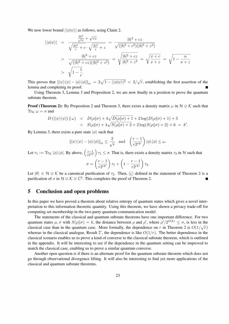
We now lower bound |〈φ|ψ〉| as follows, using Claim 2.

|〈φ|ψ〉| =|b|2√cz

+√cz√

|b|2c + c ·

√|b|2z + z

=|b|2 + cz√

(|b|2 + c2)(|b|2 + z2)

>|b|2 + cz√

(|b|2 + cz)(|b|2 + z2)=

√|b|2 + cz

|b|2 + z2=√x+ c

x+ z=√

1− α

x+ z

>

√1− 1

r.

This proves that ‖|ψ〉〈ψ| − |φ〉〈φ|‖tr = 2√

1− |〈φ|ψ〉|2 < 2/√r, establishing the first assertion of the

lemma and completing its proof.Using Theorem 3, Lemma 3 and Proposition 2, we are now finally in a position to prove the quantum

substate theorem.

Proof (Theorem 2): By Proposition 2 and Theorem 3, there exists a density matrix ω in H ⊗ K such thatTrK ω = σ and

D ((|ψ〉〈ψ|) ‖ω) < D(ρ‖σ) + 4√D(ρ‖σ) + 1 + 2 log(D(ρ‖σ) + 1) + 5

< S(ρ‖σ) + 4√S(ρ‖σ) + 2 + 2 log(S(ρ‖σ) + 2) + 6 = k′.

By Lemma 3, there exists a pure state |φ〉 such that

‖|ψ〉〈ψ| − |φ〉〈φ|‖tr ≤2√r

and(r − 1r2rk′

)|φ〉〈φ| ≤ ω.

Let τ1 := TrK |φ〉〈φ|. By above,(r−1r2rk′

)τ1 ≤ σ. That is, there exists a density matrix τ2 inH such that

σ =(r − 1r2rk′

)τ1 +

(1− r − 1

r2rk′

)τ2.

Let |θ〉 ∈ H ⊗ K be a canonical purification of τ2. Then, |ζ〉 defined in the statement of Theorem 2 is apurification of σ inH⊗K ⊗ C2. This completes the proof of Theorem 2.

5 Conclusion and open problems

In this paper we have proved a theorem about relative entropy of quantum states which gives a novel inter-pretation to this information theoretic quantity. Using this theorem, we have shown a privacy trade-off forcomputing set membership in the two-party quantum communication model.

The statements of the classical and quantum substate theorems have one important difference. For twoquantum states ρ, σ with S(ρ‖σ) = k, the distance between ρ and ρ′, where ρ′/2O(k) ≤ σ, is less in theclassical case than in the quantum case. More formally, the dependence on r in Theorem 2 is O(1/

√r)

whereas in the classical analogue, Result 2’, the dependence is like O(1/r). The better dependence in theclassical scenario enables us to prove a kind of converse to the classical substate theorem, which is outlinedin the appendix. It will be interesting to see if the dependence in the quantum setting can be improved tomatch the classical case, enabling us to prove a similar quantum converse.

Another open question is if there is an alternate proof for the quantum substate theorem which does notgo through observational divergence lifting. It will also be interesting to find yet more applications of theclassical and quantum substate theorems.

23

Acknowledgements

We are very grateful to Ashwin Nayak for his contribution to this work. He patiently went through severalversions of our proofs; his counter examples and insights were invaluable in arriving at our definition ofprivacy. We are also grateful to K. R. Parthasarathy and Rajendra Bhatia for sharing with us their insights inoperator theory.

References

[ANTV02] A. Ambainis, A. Nayak, A. Ta-Shma, and U. Vazirani. Dense quantum coding and quantumfinite automata. Journal of the ACM, 49(4):496–511, 2002.

[BBC+93] C. Bennett, G. Brassard, C. Crepeau, R. Jozsa, A. Peres, and W. Wootters. Teleporting anunknown quantum state via dual classical and Einstein-Podolsky-Rosen channels. PhysicalReview Letters, 70:1895–1899, 1993.

[BCKO93] R. Bar-Yehuda, B. Chor, E. Kushilevitz, and A. Orlitsky. Privacy, additional information, andcommunication. IEEE Transactions on Information Theory, 39(6):1930–1943, 1993.

[Bha97] R. Bhatia. Matrix Analysis. Springer-Verlag New York Inc., 1997. 2000 Reprint.

[CKGS98] B. Chor, E. Kushilevitz, O. Goldreich, and M. Sudan. Private information retrieval. Journalof the Association for Computing Machinery, 45(6):965–981, 1998.

[CR04] A. Chakrabarti and O. Regev. An optimal randomised cell probe lower bound for approxi-mate nearest neighbour searching. In Proceedings of the 45th Annual IEEE Symposium onFoundations of Computer Science, pages 473–482, 2004.

[CSWY01] A. Chakrabarti, Y. Shi, A. Wirth, and A. Yao. Informational complexity and the direct sumproblem for simultaneous message complexity. In Proceedings of the 42nd Annual IEEESymposium on Foundations of Computer Science, pages 270–278, 2001.

[CT91] T. Cover and J. Thomas. Elements of Information Theory. Wiley Series in Telecommunica-tions. John Wiley and Sons, 1991.

[CvDNT98] R. Cleve, W. van Dam, M. Nielsen, and A. Tapp. Quantum entanglement and the communi-cation complexity of the inner product function. In Proceedings of the 1st NASA InternationalConference on Quantum Computing and Quantum Communications, Lecture Notes in Com-puter Science, vol. 1509, pages 61–74. Springer-Verlag, 1998. Also quant-ph/9708019.

[FC95] C. Fuchs and C. Caves. Mathematical techniques for quantum communication theory. OpenSystems and Information Dynamics, 3(3):345–356, 1995. Also quant-ph/9604001.

[GKRdW06] D. Gavinsky, J. Kempe, O. Regev, and R. de Wolf. Bounded-error quantum state identificationand exponential separations in communication complexity. In Proceedings of the 38th AnnualACM Symposium on Theory of Computing, pages 594–603, 2006. Also quant-ph/0511013.

[Hel76] C.W. Helstrom. Quantum detection and estimation theory. Mathematics in Science and En-gineering, 123, 1976.

24

[Jai06] R. Jain. Communication complexity of remote state preparation with entanglement. QuantumInformation and Computation, 6(4–5):461–464, July 2006.

[Jai08] R. Jain. New binding-concealing trade-offs for quantum string commitment. Journal ofCryptology, 2008.

[JKN08] R. Jain, H. Klauck, and A. Nayak. Direct product theorems for classical communicationcomplexity via subdistribution bounds. In Proceedings of the 40th Annual ACM Symposiumon Theory of Computing, pages 599–608, 2008.

[Joz94] R. Jozsa. Fidelity for mixed quantum states. Journal of Modern Optics, 41(12):2315–2323,1994.

[JRS02] R. Jain, J. Radhakrishnan, and P. Sen. Privacy and interaction in quantum communicationcomplexity and a theorem about relative entropy of quantum states. In Proceedings of the43th Annual IEEE Symposium on Foundations of Computer Science, pages 429–438, 2002.

[JRS03] R. Jain, J. Radhakrishnan, and P. Sen. A direct sum theorem in communication complexityvia message compression. In Proceedings of the 30th International Conference on Automata,Languages and Programming, pages 300–315, 2003.

[JRS05] R. Jain, J. Radhakrishnan, and P. Sen. Prior entanglement, message compression and pri-vacy in quantum communication. In Proceedings of the 20th Annual IEEE Conference onComputational Complexity, pages 285–296, 2005.

[Kla00] H. Klauck. On quantum and probabilistic communication: Las Vegas and one-way protocols.In Proceedings of the 32nd Annual ACM Symposium on Theory of Computing, pages 644–651, 2000.

[Kla02] H. Klauck. On quantum and approximate privacy. In Proceedings of the 19th Annual Sympo-sium on Theoretical Aspects of Computer Science, Lecture Notes in Computer Science, vol.2285, pages 335–346. Springer-Verlag, 2002. Also quant-ph/0110038.

[Kla07] H. Klauck. One-way communication complexity and the Neciporuk lower bound on formulasize. SIAM J. Comput., 37(2):552–583, 2007.

[KNTZ07] H. Klauck, A. Nayak, A. Ta-Shma, and D. Zuckerman. Interaction in quantum communica-tion. IEEE Transactions on Information Theory, 53(6):1970–1982, June 2007.

[Low34] K. Lowner. Uber monotone Matrixfunktionen. Mathematische Zeitschrift, 38:177–216, 1934.

[MNSW98] P. B. Miltersen, N. Nisan, S. Safra, and A. Wigderson. On data structures and asymmetriccommunication complexity. Journal of Computer and System Sciences, 57(1):37–49, 1998.

[Nay99] A. Nayak. Optimal lower bounds for quantum automata and random access codes. In Pro-ceedings of the 40th Annual IEEE Symposium on Foundations of Computer Science, pages124–133, 1999.

[NC00] M. Nielsen and I. Chuang. Quantum Computation and Quantum Information. CambridgeUniversity Press, 2000.

25

[NW93] N. Nisan and A. Wigderson. Rounds in communication complexity revisited. SIAM Journalof Computing, 22:211–219, 1993.

[OR94] M. Osborne and A. Rubinstein. A course in game theory. MIT Press, 1994.

[PRV01] S. Ponzio, J. Radhakrishnan, and S. Venkatesh. The communication complexity of pointerchasing. Journal of Computer and System Sciences, 62(2):323–355, 2001.

[Ren08] R. Renner. Extracting classical randomness in a quantum world. In Proceedings of the IEEEInformation Theory Workshop, pages 360–363, 2008.

[Sch95] B. Schumacher. Quantum coding. Physical Review A, 51:2738–2747, 1995.

[Uhl76] A. Uhlmann. The “transition probability” in the state space of a ∗-algebra. Reports on Math-ematical Physics, 9(2):273–279, 1976.

[Yao93] A. C-C. Yao. Quantum circuit complexity. In Proceedings of the 34th Annual IEEE Sympo-sium on Foundations of Computer Science, pages 352–361, 1993.

A Relationships between three distinguishability measures

In this paper we have seen two measures of distinguishability between quantum states viz. relative entropyand observational divergence. The substate theorem gives a connection between observational divergenceand a third measure of distinguishability between quantum states, which we call the substate relative entropy.We define three variants of substate relative entropy below, and study the relationships between them andrelative entropy and observational divergence.

Definition 11 (Substate relative entropy) Let ρ, σ be two quantum states in the same Hilbert space H.The state ρ is said to have the k-substate property with respect to σ if for all r ≥ 1, there exists a quantumstate ρ(r) in H such that ‖ρ− ρ(r)‖tr ≤

2r and

(r−1r2rk

)ρ(r) ≤ σ. The state ρ is said to have the weak

k-substate property with respect to σ if ‖ρ− ρ(r)‖tr is upper bounded by 2√r

instead of 2r . The state ρ is

said to have the strong k-substate property with respect to σ if ρ2k≤ σ. The substate relative entropy of ρ

with respect to σ, S sub(ρ‖σ), is defined to be the infimum over k such that ρ has the k-substate propertywith respect to σ. The quantities strong substate relative entropy, S sub,strong , and weak substate relativeentropy, S sub,weak , are defined analogously.

Remark: The classical version of strong substate relative entropy was also defined by Jain, Klauck andNayak [JKN08] where they call it relative co-min entropy. The strong substate relative entropy was alsodefined by Renner in [Ren08] where it is called relative min-entropy. Our definitions of substate relativeentropy and weak substate relative entropy are similar, but actually incomparable, to the smooth relativemin-entropy defined in [Ren08].

The next proposition lists some easy properties of substate relative entropy.

Proposition 3 Let ρ, σ be density matrices in the same Hilbert spaceH. Then,

1. S sub(ρ‖σ) ≥ 0, with equality iff ρ = σ;

2. S sub(ρ‖σ) <∞ iff supp(ρ) ⊆ supp(σ);

26

3. S sub(·‖·) is continuous in its two arguments over the domain of pairs of full-support states;

4. (Unitary invariance) If U is a unitary transformation onH, S sub(UρU †‖UσU †) = S sub(ρ‖σ);

5. (Monotonicity) Suppose K is a Hilbert space, and ρ′, σ′ are extensions of ρ, σ in H ⊗ K. Then,S sub(ρ‖σ) ≤ S sub(ρ′‖σ′). This implies, via unitary invariance and the Kraus representation theo-rem, that if T is a completely positive trace preserving superoperator from H to a Hilbert space L,then S sub(T ρ‖T σ) ≤ S sub(ρ‖σ).

Analogous statements hold for S sub,weak and S sub,strong also.

The following proposition states various relationships between our three measures of distinguishabilitythat we have mentioned earlier.

Proposition 4 Let P,Q be two probability distributions on [n] and ρ, σ be two quantum states in Cn. Then,

1. (Classical substate theorem) S sub(P‖Q) ≤ D(P‖Q);

2. (Quantum substate theorem) S sub,weak (ρ‖σ) ≤ D(ρ‖σ)+4√D(ρ‖σ) + 1+2 log(D(ρ‖σ)+1)+5;

3. D(ρ‖σ) ≤ 2S sub(ρ‖σ) + 2;

4. S(ρ‖σ) ≤ S sub,strong(ρ‖σ);

5. D(P‖Q)− 1 ≤ S(P‖Q) ≤ D(P‖Q)(n− 1).

6. D(ρ‖σ)− 1 ≤ S(ρ‖σ) ≤ D(ρ‖σ)(n− 1) + log n.

7. There exist probability distributions P,Q on [n] such that S(P‖Q) >(D(P‖Q)

2 − 1)

(n− 2)− 1.

8. There exists a two-outcome POVM F on Cn such that S(ρ‖σ) ≥ S(Fρ‖Fσ) ≥ S(ρ‖σ)−lognn−1 − 1.

Remarks:1. From Parts 1 and 3 of Proposition 4, we see that the classical substate theorem (Result 2’) has a converse.2. Unfortunately, we are unable to prove a converse to the quantum substate theorem (Result 2) as Part 2 ofProposition 4 only guarantees a weak substate property between the two quantum states ρ, σ.3. Part 8 of Proposition 4 is a counterpart to monotonicity of relative entropy (Fact 4).

Proof (Proposition 4):

1. Define k := D(P‖Q). Without loss of generality, k > 0. Let r ≥ 1. Define the set Bad := i ∈ [n] :P (i)/2rk > Q(i). Then,

k = D(P‖Q) ≥ P (Bad) logP (Bad)Q(Bad)

> P (Bad) · rk ⇒ P (Bad) <1r,

which is the same as expression (3) in Section 1.2. We can now argue similarly as in the proof ofResult 2’ to prove Part 1 of the present proposition.

2. Follows from Theorem 3 and Lemma 3.

27

3. Without loss of generality, 0 < k1 := D(ρ‖σ) < +∞. Let F be a POVM element in Cn such that

k1 = p log(p/q)⇒ q =p

2k1/p,

where p := Tr (Fρ) and q := Tr (Fσ). Note that p > 0. Let r := 2/p. Since ρ, σ have the k-substateproperty, let ρ′ be the quantum state in Cn such that ‖ρ− ρ′‖tr ≤

2r = p and

(r−1r2rk

)ρ′ ≤ σ. Define

p′ := Tr (Fρ′). Then, p′ ≥ p/2. Also,

p

2k1/p= q = Tr (Fσ) ≥

(1− r−1

2rk

)Tr (Fρ′) =

(1− p

2

) p′

2rk

≥ p

2rk+2.

The last inequality above follows because p ≤ 1 and p′ ≥ p/2. This implies that

rk + 2 ≥ k1

p⇒ p(rk + 2) ≥ k1 ⇒ 2k + 2 ≥ k1,

where the second implication follows because p ≤ 1 and p = 2/r. This completes the proof of Part 3of the present proposition.

4. Without loss of generality, k < +∞. We have

S(ρ‖σ) = Tr ρ log ρ− Tr ρ log σ ≤ Tr ρ log ρ− Tr ρ logρ

2k= k · Tr ρ = k.

The inequality above is by monotonicity of the logarithm function on positive operators [Low34].

5. Without loss of generality, 0 < D(P‖Q) < +∞. The lower bound on S(P‖Q) was proved inProposition 2. Define xi = log(pi/qi). We can assume without loss of generality, by perturbing Qslightly, that the values xi are distinct for distinct i. Let S′ = i : xi > 0. Let k := D(P‖Q). LetFor all positive l, define Sl := i ∈ [n] : xi ≥ l. Therefore,

k ≥ PrP

[Sl] logPrP [Sl]PrQ[Sl]

≥ PrP

[Sl]l⇒ PrP

[Sl] ≤ k/l.

Assume without loss of generality that x1 < x2 < · · · < xn. Then if xi > 0, PrP [Sxi ] ≤ k/xi.Since S(P‖Q) ≤

∑i∈S′ pixi, the upper bound on S(P‖Q) is maximised when S′ = 2, . . . , n,

pn = k/xn, pi = k(1/xi − 1/xi+1) for all i ∈ 2, . . . , n− 1, and p1 = 1−∑n

i=2 pi. Then,

S(P‖Q) ≤n∑i=2

pixi = kn−1∑i=2

xi(1/xi − 1/xi+1) + k = kn−1∑i=2

xi+1 − xixi+1

+ k ≤ kn−1∑i=2

1 + k

= k(n− 1).

6. Without loss of generality, 0 < D(ρ‖σ) < +∞. The lower bound on S(ρ‖σ) was proved in Proposi-tion 2. Let us measure ρ and σ in the eigenbasis of σ. We get two distributions, P and Q. Below, wewill sometimes think of P,Q as diagonal density matrices. From Part 5 of the present proposition, itfollows that

D(P‖Q)(n− 1) ≥ S(P |Q) = Tr (P logP )− Tr (P logQ) ≥ − log n− Tr (P logQ)= − log n− Tr (ρ log σ) = − log n+ S(ρ‖σ)− Tr (ρ log ρ)≥ − log n+ S(ρ‖σ).

28

The second equality above holds since the measurement was in the eigenbasis of σ.

Thus,S(ρ‖σ) ≤ D(P‖Q)(n− 1) + log n ≤ D(ρ‖σ)(n− 1) + log n,

where the second inequality is by monotonicity of observational divergence (Proposition 1).

7. Fix a > 1, k > 0. Define for all i ∈ 1, . . . , n − 1, pi := a−i(a − 1), and pn := a−(n−1).Define for all i ∈ 2, . . . , n, qi := pi2−ka

i−1, and q1 := 1 −

∑ni=2 qi. Define P := (p1, . . . , pn),

Q := (q1, . . . , qn); P,Q are probability distributions on [n]. For any r > 1, define P to be thevector (p1, . . . , pdloga re, 0, . . . , 0) normalised in order to make it a probability distribution on [n] (if

r > an−1, there is no suffix of zeroes in the definition of P ). It is easy to see that∥∥∥P − P∥∥∥

1≤ 2/r

and (r−1)Pr2rk

≤ Q. This shows that S sub(P‖Q) ≤ k; hence D(P‖Q) ≤ 2(k + 1) by Part 3 of thepresent proposition.

Now,

S(P‖Q) =n∑i=1

pi logpiqi≥ p1 log p1 +

n∑i=2

pi logpiqi

> −0.9 + (n− 2)k(a− 1)

a+ k

= k(n− 1)− k(n− 2)a

− 0.9.

The second inequality above follows because p log p > −0.9 for all 0 ≤ p ≤ 1. By choosing a largeenough, we can achieve S(P‖Q) > k(n − 1) − 1. This completes the proof of Part 7 of the presentproposition.

8. The upper bound on S(Fρ‖Fσ) follows from the monotonicity of relative entropy (Fact 4). Withoutloss of generality, 0 < S(ρ‖σ) < +∞. We know that there exists a POVM element F in Cn suchthat D(ρ‖σ) = p log(p/q), where p := Tr Fρ and q := Tr Fσ. Define the two-outcome POVM Fon Cn to be (F, 11 − F ), where 11 is the identity operator on Cn. Then, the probability distributionsFρ = (p, 1− p) and Fσ = (q, 1− q). Note that

S(Fρ‖Fσ) = p logp

q+ (1− p) log

1− p1− q

> p logp

q− 1 = D(ρ‖σ)− 1,

where the inequality follows because x log x > −1 for all 0 ≤ x ≤ 1. From Part 6 of the presentproposition, it follows that

S(ρ‖σ) ≤ D(ρ‖σ)(n− 1) + log n ≤ (S(Fρ‖Fσ) + 1)(n− 1) + log n

⇒ S(Fρ‖Fσ) ≥ S(ρ‖σ)− log nn− 1

− 1.

29