A new dynamical approach of Emden-Fowler equations andsystems

Marie Françoise BIDAUT-VERON∗ Hector GIACOMINI†

.

Abstract

We give a new approach on general systems of the form

(G)

−∆pu = −div(|∇u|p−2∇u) = ε1 |x|a usvδ,−∆qv = −div(|∇v|q−2∇u) = ε2 |x|b uµvm,

where Q, p, q, δ, µ, s,m, a, b are real parameters, Q, p, q 6= 1, and ε1 = ±1, ε2 = ±1. In theradial case we reduce the problem to a quadratic system of four coupled first order autonomousequations, of Kolmogorov type. It allows to obtain new local and global existence or nonexistenceresults. We consider in particular the case ε1 = ε2 = 1.We describe the behaviour of the groundstates in two cases where the system is variational. We give a result of existence of ground statesfor a nonvariational system with p = q = 2 and s = m > 0, that improves the former ones.It is obtained by introducing a new type of energy function. In the nonradial case we solvea conjecture of nonexistence of ground states for the system with p = q = 2, δ = m + 1 andµ = s+ 1.

Keywords Elliptic quasilinear systems. Variational or nonvariational problems. Autonomousand quadratic systems. Stable manifolds. Heteroclinic orbits.

A.M.S. Subject Classification 34B15, 34C20, 34C37; 35J20, 35J55, 35J65, 35J70; 37J45.

.∗Laboratoire de Mathématiques et Physique Théorique, CNRS UMR 6083, Faculté des Sciences, 37200 Tours

France. E-mail address:veronmf@univ-tours.fr†Laboratoire de Mathématiques et Physique Théorique, CNRS UMR 6083, Faculté des Sciences, 37200 Tours

France. E-mail address:Hector.Giacomini@lmpt.univ-tours.fr

1

1 Introduction

In this paper we consider the nonnegative solutions of Emden-Fowler equations or systems inRN (N = 1),

−∆pu = −div(|∇u|p−2∇u) = ε1 |x|a uQ, (1.1)

(G)

−∆pu = −div(|∇u|p−2∇u) = ε1 |x|a usvδ,−∆qv = −div(|∇v|q−2∇u) = ε2 |x|b uµvm,

(1.2)

where Q, p, q, δ, µ, s,m, a, b are real parameters, Q, p, q 6= 1, and ε1 = ±1, ε2 = ±1. These problemsare the subject of a very rich litterature, either in the case of source terms (ε1 = ε2 = 1) orabsorption terms (ε1 = ε2 = 1) or mixed terms (ε1 = −ε2). In the sequel we are concerned by theradial solutions, except at Section 9 where the solutions may be nonradial.

In this article we we give a new way of studying the radial solutions. In Section 2 we reducesystem (G) to a quadratic autonomous system:

(M)

Xt = X

[X − N−p

p−1 + Zp−1

],

Yt = Y[Y − N−q

q−1 + Wq−1

],

Zt = Z [N + a− sX − δY − Z] ,Wt = W [N + b− µX −mY −W ] ,

where t = ln r, and

X(t) = −ru′

u, Y (t) = −rv

′

v, Z(t) = −ε1r

1+ausvδu′

|u′|p , W (t) = −ε2r1+buµvm

v′

|v′|q . (1.3)

This system is of Kolmogorov type. The reduction is valid for equations and systems with sourceterms , absorption terms , or mixed terms . It is remarkable that in the new system, p and q appearonly as simple coeffi cients, which allows to treat any value of the parameters, even p or q < 1, ands,m, δ or µ < 0.

In Section 3 we revisit the well-known scalar case (1.1), where (G) becomes two-dimensional. Weshow that the phase plane of the system gives at the same time the behaviour of the two equations

−∆pu = |x|a uQ and −∆pu = − |x|a uQ,

which is a kind of unification of the two problems, with source terms or absorption terms. For thecase of source term (ε1 = 1), we find again the results of [2], [19], showing that the new dynamicalapproach is simple and does not need regularity results or energy functions. Moreover it gives amodel for the study of system (G). Indeed if p = q, a = b and δ + s = µ + m, system (G) admitssolutions of the form (u, u), where u is a solution of (1.1) with Q = δ + s.

In the sequel of the article we study the case of source terms, i.e. (G) = (S), where

(S)

−∆pu = |x|a usvδ,−∆qv = |x|b uµvm. (1.4)

This system has been studied by many authors, in particular the Hamiltonian problem s = m = 0,in the linear case p = q = 2, see for example [20], [31], [29], [9], [33], [14], and the potential system

2

where δ = m+ 1, µ = s+ 1 and a = b, see [7], [34], [35]; the problem with general powers has beenstudied in [3], [39], [40], [41] in the linear case and [6], [12], [42] in the quasilinear case, see also [1],[10], [13].

Here we suppose that δ, µ > 0, so that the system is always coupled, s,m = 0, and we assumefor simplicity

1 < p, q < N, min(p+ a, q + b) > 0, D = δµ− (p− 1− s)(q − 1−m) > 0. (1.5)

We say that a positive solution (u, v) in (0, R) is regular at 0 if u, v ∈ C2 (0, R)∩C([0, R)). Conditionmin(p+a, q+b) > 0 guaranties the existence of local regular solutions. Then u, v ∈ C1([0, R)). whena, b > −1, and u′(0) = v′(0) = 0. The assumption D > 0 is a classical condition of superlinearityfor the system.

We are interessed in the existence or nonexistence of ground states, called G.S., that meansglobal positive (u, v) in (0,∞) and regular at 0. We exclude the case of "trivial" solutions, (u, v) =(0, C) or (C, 0) , where C is a constant, which can exist when s > 0 or m > 0.

In Section 4 we give a series of local existence or nonexistence results concerning system (S),which complete the nonexistence results found in the litterature. They are not based on the fixedpoint method, quite hard in general, see for example [19], [27]. We make a dynamical analysis ofthe linearization of system (M) near each fixed point, which appears to be performant, even forthe regular solutions. For a better exposition, the proofs are given at Section 10.

In Section 5 we study the global existence of G.S. This problem has been often compared withthe nonexistence of positive solutions of the Dirichlet problem in a ball, see [29], [30], [12], [13]. Herewe use a shooting method adapted to system (M), which allows to avoid questions of regularity ofsystem (S). We give a new way of comparison, and improve the former results:

Theorem 1.1 (i) Assume s < N(p−1)+p+paN−p and m < N(q−1)+q+qb

N−q . If system (S) has no G.S., then

(i) there exist regular radial solutions such that X(T ) = N−pp−1 and Y (T ) = N−q

q−1 for some T > 0,

with 0 < X < N−pp−1 and 0 < Y < N−q

q−1 on (−∞, T ).

(ii) there exists a positive radial solution (u, v) of the Dirichlet problem in a ball B(0, R).

This result is a key tool in the next Sections for proving the existence of a G.S. It gives alsonew existence results for the Dirichlet problem, see Corollary 5.3. We also give a complementaryresult:

Proposition 1.2 Assume s = N(p−1)+p+paN−p and m = N(q−1)+q+qb

N−q . Then all the regular radialsolutions are G.S.

In Section 6 we study the radial solutions of the well known Hamiltonian system

(SH)

−∆u = |x|a vδ,−∆v = |x|b uµ,

corresponding to p = q = 2 < N, s = m = 0, a > −2, which is variational. In the case a = b = 0, amain conjecture was made in [32]:

3

Conjecture 1.3 System (SH) with a = b = 0 admits no (radial or nonradial) G.S. if and only if(δ, µ) is under the hyperbola of equation

N

δ + 1+

N

µ+ 1= N − 2.

The question is still open; it was solved in the radial case in [26], [29], then partially in [31], [9],and up to the dimension N = 4 in [33], see references therein. Here we find again and extend tothe case a, b 6= 0 some results of [20] relative to the G.S., with a shorter proof. We also give anexistence result for the Dirichlet problem improving a result of [14].

Theorem 1.4 Let H0 be the critical hyperbola in the plane (δ, µ) defined by

N + a

δ + 1+N + b

µ+ 1= N − 2. (1.6)

Then(i) System (SH) admits a (unique) radial G.S. if and only if (δ, µ) is above H0 or on H0.

(ii) The radial Dirichlet problem in a ball has a solution if and only if (δ, µ) is under H0.

(iii) On H0 the G.S. has the following behaviour at ∞ : assuming for example δ > N+aN−2 , then

limr→∞ rN−2u(r) = α > 0, and

limr→∞

r(N−2)µ−(2+b)v = β > 0 if µ <N + b

N − 2,

limr→∞

rN−2v = β > 0 if µ >N + b

N − 2,

limr→∞

rN−2 |ln r|−1 v = β > 0 if µ =N + b

N − 2.

Our proofs use a Pohozaev type function; in terms of the new variables X,Y, Z,W , it containsa quadratic factor

EH(r) = rN

[u′v′ + rb

|u|µ+1

µ+ 1+ ra

|v|δ+1

δ + 1+N + a

δ + 1

vu′

r+N + b

µ+ 1

uv′

r

]

= rN−2uv

[XY − Y (N + b−W )

µ+ 1− (N + a− Z)X

δ + 1

]. (1.7)

As observed in ([20]) the G.S. can present a non-symmetric behaviour. This non-symmetry phe-nomena has to be taken in account for solving conjecture (1.3).

In Section 7 we consider the radial solutions of a nonvariational system:

(SN)

−∆u = |x|a usvδ,−∆v = |x|a uµvs,

where p = q = 2 < N, a = b > −2 and m = s > 0. For small s it appears as a perturbation ofsystem (SH). In the litterature very few results are known for such nonvariational systems. Ourmain result in this Section is a new result of existence of G.S . valid for any s:

4

Theorem 1.5 Consider the system (SN), with N > 2, a > −2. We define a curve Cs in the plane(δ, µ) by

N + a

µ+ 1+N + a

δ + 1= N − 2 +

(N − 2)s

2min(

1

µ+ 1,

1

δ + 1), (1.8)

located under the hyperbola defined by (1.6). If (δ, µ) is above Cs, system (SN) admits a G.S.

This result is obtained by constructing a new type of energy function which contains two terms inX2, Y 2 :

Φ(r) = rN[u′v′ + rb

uµ+1vs

µ+ 1+ ra

usvδ+1

δ + 1+N + a

δ + 1

vu′

r+N + b

µ+ 1

uv′

r+

s

2(δ + 1)

vu′2

u+

s

2(µ+ 1)

uv′2

v

]= rN−2uv

[XY − Y (N + b−W )

µ+ 1− (N + a− Z)X

δ + 1+

s

2(δ + 1)X2 +

s

2(µ+ 1)Y 2

]. (1.9)

In Section 8 we consider the radial solutions of the potential system

(SP )

−∆pu = |x|a usvm+1,−∆qv = |x|a us+1vm,

where δ = m + 1, µ = s + 1 and a = b, which is variational, see [34], [35]. Using system (M) wededuce new results of existence:

Theorem 1.6 Let D be the critical line in the plane (m, s) defined by

N + a = (m+ 1)N − qq

+ (s+ 1)N − pp

.

Then(i) System (SP ) admits a radial G.S. if and only if (m, s) is above or on D.

(ii) On D the G.S. has the following behaviour: suppose for example q 5 p. Let λ∗ = N + a −(s+ 1)N−pp−1 −m

N−qq−1 . Then limr→∞ r

N−pp−1 u(r) = α > 0, and

limr→∞

rN−qq−1 v(r) = β > 0 if λ∗ < 0, (1.10)

limr→∞

r

N−pp−1 µ−(q+b)q−1−m v(r) = β > 0 if λ∗ > 0, (1.11)

limr→∞

rN−qq−1 |ln r|−

1q−1−m v(r) = β > 0 if λ∗ = 0. (1.12)

In particular (1.10) holds if p = q, or q 5 m+ 1.

(iii) The radial Dirichlet problem in a ball has a solution if and only if (m, s) is under D.

5

In that case we use the following energy function, which deserves to be compared with the oneof Section 6 , since it has also a quadratic factor:

EP (r) = rN

[(s+ 1)(

|u′|p

p′+N − pp

u |u′|p−2 u′

r) + (m+ 1)(

|v′|q

q′+N − qq

v |v′|q−2 v′

r) + raus+1vm+1

]

= rN−2−a |u′|p−1 |v′|q−1

usvm

[ZW − (s+ 1)W (N − p− (p− 1)X)

p− (m+ 1)Z(N − q − (q − 1)Y )

q

].

(1.13)

Finally in Section 9 we deduce a nonradial result for the potential system in the case of twoLaplacians:

(SL)

−∆u = |x|a usvm+1,−∆v = |x|a us+1vm.

Our result proves a conjecture proposed in [7], showing that in the subcritical case there exists noG.S.:

Theorem 1.7 Assume a > −2 and s,m = 0. If

s+m+ 1 < min(N + 2

N − 2,N + 2 + 2a

N − 2), (1.14)

then system (SL) admits no (radial or nonradial) G.S.

Our proof uses the estimates of [7], which up to now are the only extensions of the results of[18] to systems. It is based on the construction of a nonradial Pohozaev function extending theradial one given at (1.13) for p = q = 2, different from the energy function used in [7].

The case of the system (G) with absorption terms (ε1 = ε2 = −1) or mixed terms (ε1 = −ε2 =1), studied in [4], [5], will be the subject of a second article. Our approach also extends to a systemwith gradient terms and doubly singular:

−div(|x|c uρ |∇u|p−2∇u) = ε1 |x|a usvδ |∇u|η |∇v|` ,−div(|x|d vλ |∇v|p−2∇v) = ε2 |x|b uµvm |∇u|ν |∇v|κ ,

(1.15)

which will be studied in another work.

Acknoledgment The authors are grateful to Raul Manasevich whose stimulating discussionsencouraged us to study system (G).

2 Reduction to a quadratic system

2.1 The change of unknowns

Here we consider the radial positive solutions r 7→ (u(r), v(r)) of system (G) on any interval(R1, R2), that means

(|u′|p−2 u′

)′+ N−1

r |u′|p−2 u′ = r1−N

(rN−1 |u′|p−2 u′

)′= −ε1r

ausvδ,(|v′|q−2 v′

)′+ N−1

r |v′|q−2 v′ = r1−N

(rN−1 |v′|p−2 v′

)′= −ε2r

buµvm.

6

Near any point r where u(r) 6= 0, u′(r) 6= 0 and v(r) 6= 0, v′(r) 6= 0 we define

X(t) = −ru′

u, Y (t) = −rv

′

v, Z(t) = −ε1r

1+ausvδ∣∣u′∣∣−p u′, W (t) = −ε2r

1+buµvm∣∣v′∣∣−q v′,

(2.1)where t = ln r. Then we find the system

(M)

Xt = X

[X − N−p

p−1 + Zp−1

],

Yt = Y[Y − N−q

q−1 + Wq−1

],

Zt = Z [N + a− sX − δY − Z] ,Wt = W [N + b− µX −mY −W ] .

This sytem is quadratic, and moreover a very simple one, of Kolmogorov type: it admits fourinvariant hyperplanes: X = 0, Y = 0, Z = 0,W = 0. As a first consequence all the fixed pointsof the system are explicite. The trajectories located on these hyperplanes do not correspond to asolution of system (G); they will be called nonadmissible.

We suppose that the discriminant of the system

D = δµ− (p− 1− s)(q − 1−m) 6= 0. (2.2)

Then one can express u, v in terms of the new variables:

u=r−γ( |X|p−1 |Z|)(q−1−m)/D( |Y |q−1 |W |)δ/D, v=r−ξ( |X|p−1 |Z|)µ/D( |Y |q−1 |W |)(p−1−s)/D,(2.3)

where γ and ξ are defined by

γ =(p+ a)(q − 1−m) + (q + b)δ

D, ξ =

(q + b)(p− 1− s) + (p+ a)µ

D, (2.4)

or equivalently by

(p− 1− s)γ + p+ a = δξ, (q − 1−m)ξ + q + b = µγ. (2.5)

Since system (M) is autonomous, each admissible trajectory T in the phase space corresponds toa solution (u, v) of system (G) unique up to a scaling: if (u, v) is a solution, then for any θ > 0,r 7→ (θγu(θr), θξv(θr)) is also a solution.

2.2 Fixed points of system (M)

System (M) has at most 16 fixed points. The main fixed point is

M0 = (X0, Y0, Z0,W0) = (γ, ξ,N − p− (p− 1)γ,N − q − (q − 1)ξ) , (2.6)

corresponding to the particular solutions

u0(r) = Ar−γ , v0(r) = Br−ξ, A,B > 0, (2.7)

7

when they exist, depending on ε1, ε2. The values of A and B are given by

AD =(ε1γ

p−1(N − p− γ(p− 1)))q−1−m (

ε2ξq−1(N − q − (q − 1)ξ)

)δ,

BD =(ε2ξ

q−1(N − q − (q − 1)ξ))p−1−s (

ε1γp−1(N − p− (p− 1)γ)

)µ.

The other fixed points are

0 = (0, 0, 0, 0), N0 = (0, 0, N + a,N + b), A0 = (N − pp− 1

,N − qq − 1

, 0, 0),

I0 = (N − pp− 1

, 0, 0, 0), J0 = (0,N − qq − 1

, 0, 0), K0 = (0, 0, N + a, 0), L0 = (0, 0, 0, N + b),

G0 = (N − pp− 1

, 0, 0, N + b− N − pp− 1

µ), H0 = (0,N − qq − 1

, N + a− N − qq − 1

δ, 0),

and if m 6= q − 1,

P0 = (N − pp− 1

,

N−pp−1 µ− (q + b)

q − 1−m , 0,(q − 1)(N + b− N−p

p−1 µ)−m(N − q)q − 1−m ),

C0 =

(0,− q + b

q − 1−m, 0,(N + b)(q − 1)−m(N − q)

q − 1−m

),

R0 =

(0,− q + b

q − 1−m,N + a+ δb+ q

q − 1−m,(N + b)(q − 1)−m(N − q)

q − 1−m

),

and by symmetry, if s 6= p− 1,

Q0 = (

N−qq−1 δ − (p+ a)

p− 1− s ,N − qq − 1

,(p− 1)(N + a− N−q

q−1 δ)− s(N − p)p− 1− s , 0),

D0 =

(− p+ a

p− 1− s, 0,(N + a)(p− 1)− s(N − p)

p− 1− s , 0

),

S0 =

(− p+ a

p− 1− s, 0,(N + a)(p− 1)− s(N − p)

p− 1− s ,N + b+ µa+ p

p− 1− s

).

2.3 First comments

Remark 2.1 This formulation allows to treat more general systems with signed solutions by re-ducing the study on intervals where u and v are nonzero. Consider for example the problem

−∆pu = ε1 |x|a |u|s |v|δ−1 v, −∆qv = ε2 |x|b |v|m |u|µ−1 u.

0n any interval where uv > 0, the couple (|u| , |v|) is a solution of (G). On any interval whereu > 0 > v, the couple (u, |v|) satisfies (G) with (ε1, ε2) replaced by (−ε1,−ε2).

Remark 2.2 There is another way for reducing the system to an autonomous form: setting

U(t) = rγu, V(t) = rξv, H(t) = −r(γ+1)(p−1)∣∣u′∣∣p−2

u′, K(t) = −r(ξ+1)(q−1)∣∣v′∣∣q−2

v′,

8

with t = ln r, we findUt = γU− |H|(2−p)/(p−1) H, Vt = ζU− |K|(2−q)/(q−1) K,

Ht = (γ(p− 1) + p−N)H + ε1UsVδ, Kt = (ζ(q − 1) + q −N)K + ε2UµVm.(2.8)

It extends the well-known transformation of Emden-Fowler in the scalar case when p = 2, used alsoin [2] for general p, see Section 3. When p = q = 2 we obtain

Utt + (N − 2− 2γ)Ut − γ(N − 2− γ)U + ε1UsVδ = 0,Vtt + (N − 2− 2ξ)Vt − ξ(N − 2− ξ)V + ε2UµVm = 0,

(2.9)

which was extended to the nonradial case and used for Hamiltonian systems (s = m = 0), withsource terms in [9] (ε1 = ε2 = 1) and absorption terms in [4] (ε1 = ε2 = −1). Our system is moreadequated for finding the possible behaviours: unlike system (2.8)it has no singularity, since it ispolynomial, also its fixed points at ∞ are not concerned when we deal with solutions u, v > 0.

Remark 2.3 In the specific case p = q = 2, setting

z = XZ = ε1r2+a |u|s−2 u |v|δ−1 v, w = YW = ε2r

2+b |u|µ−1 u |v|m−2 v,

we get the following systemXt = X2 − (N − 2)X + z, Yt = Y 2 − (N − 2)Y + w,

zt = z [2 + a+ (1− s)X − δY ] , wt = w [2 + b− µX + (1−m)Y ] .

It has been used in [20] for studying the Hamiltonian system (SH). Even in that case we will showat Section 6 that system (M) is more performant, because it is of Kolmogorov type.

Remark 2.4 Assume p = q and a = b. Setting t = kt and(X, Y , Z, W

)= k(X,Y, Z,W ), we

obtain a system of the same type with N, a replaced by N , a, with

N − pN − p = k =

N + a

N + a.

It corresponds to the change of unknowns

r = rk, u(r) = C1u(r), v(r) = C2u(r), C1 = kp(p−1−m+δ)/D, C2 = k(p(p−1−s+µ))/D.

From (2.3) and (2.4), we get γ/γ = ξ/ξ = k = p+ap+a . There is one free parameter. In particular

1) we get a system without power (a = 0), by taking

N =p(N + a)

p+ a, k =

p

p+ a;

2) we get a system in dimension N = 1, by taking

k = − p− 1

N − p < 0, , a =p+ a− (N + a)p

N − p .

9

3 The scalar case

We first study the signed solutions of two scalar equations with source or absorption:

−∆pu = −r1−N(rN−1

∣∣u′∣∣p−2u′)′

= ε |x|a |u|Q−1 u, (3.1)

with ε = ±1, 1 < p < N, Q 6= p− 1 and p+ a > 0.

We cannot quote all the huge litterature concerning its solutions, supersolutions or subsolutions,from the first studies of Emden and Fowler for p = 2, recalled in [16]; see for example [2] and [37],for any p > 1, and references therein. We set

Q1 =(N + a)(p− 1)

N − p , Q2 =N(p− 1) + p+ pa

N − p , γ =p+ a

Q+ 1− p.

From Remark 2.4 we could reduce the system to the case a = 0, in dimension N = p(N+a)/(p+a).However we do not make the reduction, because we are motivated by the study of system (G), andalso by the nonradial case.

3.1 A common phase plane for the two equations

Near any point r where u(r) 6= 0 (positive or negative), and u′(r) 6= 0 setting

X(t) = −ru′

u, Z(t) = −εr1+a |u|Q−1 u

∣∣u′∣∣−p u′, (3.2)

with t = ln r, we get a 2-dimensional system

(Mscal)

Xt = X

[X − N−p

p−1 + Zp−1

],

Zt = Z [N + a−QX − Z] .

and then |u|=r−γ( |Z| |X|p−1)1/(Q+1−p). This change of unknown was mentioned in [11] in the casep = 2, ε = 1 and N = 3. It is remarkable that system (Mscal) is the same for the two cases ε = ±1,the only difference is that X(t)Z(t) has the sign of ε :

The equation with source (ε = 1) is associated to the 1st and 3rd quadrant. It is well known thatany local solution has a unique extension on (0,∞) . The 1st quadrant corresponds to the intervalswhere |u| is decreasing, which can be of the following types (0,∞) , (0, R2),(R1,∞),(R1, R2), 0 <R1 < R2 <∞. The 3rd quadrant corresponds to the intervals (R1, R2) where |u| is increasing.

The equation with absorption (ε = −1) is associated to the 2nd and 4th quadrant. It isknown that the solutions have at most one zero, and their maximal interval of existence can be(0, R2), (R1,∞), (R1, R2) or (0,∞). The 2nd quadrant corresponds to the intervals (R1, R2) where|u| is increasing. The 4th quadrant corresponds to the intervals (0, R2) or (R1,∞) where |u| isdecreasing.

The fixed points of (Mscal) are

M0 = (X0, , Z0) = (γ,N − p− (p− 1)γ), (0, 0), N0 = (0, N + a), A0 = (N − pp− 1

, 0).

10

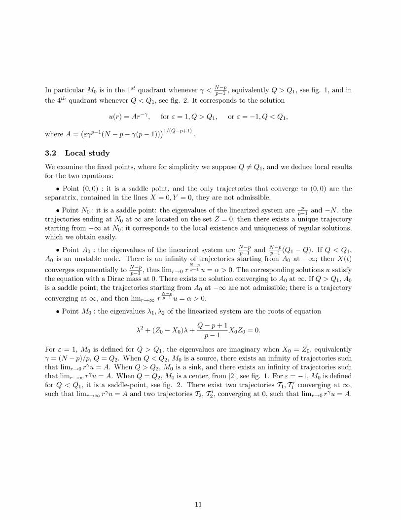
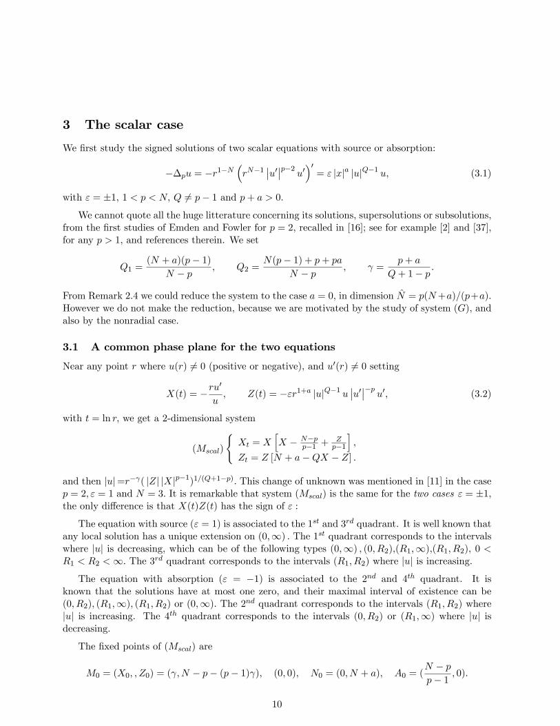
In particular M0 is in the 1st quadrant whenever γ <N−pp−1 , equivalently Q > Q1, see fig. 1, and in

the 4th quadrant whenever Q < Q1, see fig. 2. It corresponds to the solution

u(r) = Ar−γ , for ε = 1, Q > Q1, or ε = −1, Q < Q1,

where A =(εγp−1(N − p− γ(p− 1))

)1/(Q−p+1).

3.2 Local study

We examine the fixed points, where for simplicity we suppose Q 6= Q1, and we deduce local resultsfor the two equations:

• Point (0, 0) : it is a saddle point, and the only trajectories that converge to (0, 0) are theseparatrix, contained in the lines X = 0, Y = 0, they are not admissible.

• Point N0 : it is a saddle point: the eigenvalues of the linearized system are pp−1 and −N . the

trajectories ending at N0 at ∞ are located on the set Z = 0, then there exists a unique trajectorystarting from −∞ at N0; it corresponds to the local existence and uniqueness of regular solutions,which we obtain easily.

• Point A0 : the eigenvalues of the linearized system are N−pp−1 and N−p

p−1 (Q1 − Q). If Q < Q1,A0 is an unstable node. There is an infinity of trajectories starting from A0 at −∞; then X(t)

converges exponentially to N−pp−1 , thus limr→0 r

N−pp−1 u = α > 0. The corresponding solutions u satisfy

the equation with a Dirac mass at 0. There exists no solution converging to A0 at∞. If Q > Q1, A0

is a saddle point; the trajectories starting from A0 at −∞ are not admissible; there is a trajectory

converging at ∞, and then limr→∞ rN−pp−1 u = α > 0.

• Point M0 : the eigenvalues λ1, λ2 of the linearized system are the roots of equation

λ2 + (Z0 −X0)λ+Q− p+ 1

p− 1X0Z0 = 0.

For ε = 1, M0 is defined for Q > Q1; the eigenvalues are imaginary when X0 = Z0, equivalentlyγ = (N − p)/p, Q = Q2. When Q < Q2, M0 is a source, there exists an infinity of trajectories suchthat limr→0 r

γu = A. When Q > Q2, M0 is a sink, and there exists an infinity of trajectories suchthat limr→∞ rγu = A. When Q = Q2, M0 is a center, from [2], see fig. 1. For ε = −1, M0 is definedfor Q < Q1, it is a saddle-point, see fig. 2. There exist two trajectories T1, T ′1 converging at ∞,such that limr→∞ rγu = A and two trajectories T2, T ′2 , converging at 0, such that limr→0 r

γu = A.

11

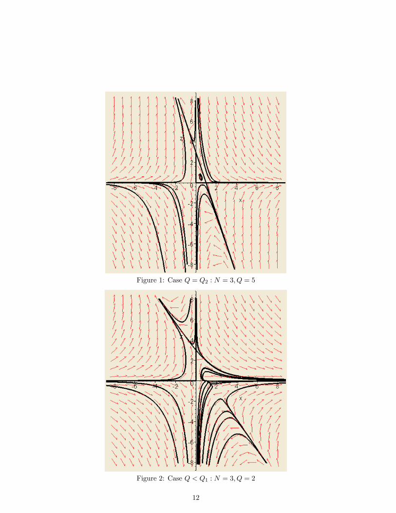
Figure 1: Case Q = Q2 : N = 3, Q = 5

Figure 2: Case Q < Q1 : N = 3, Q = 2

12

3.3 Global study

Remark 3.1 System (Mscal) has no limit cycle for Q 6= Q2. It is evident when ε = −1. Whenε = 1, as noticed in [19], it comes from the Dulac’s theorem: setting Xt = f(X,Z), Zt = g(X,Z),and

B(X,Z) = XpQ/(Q+1−p)−2Z(p/(Q+1−p)−1, M = BXXt +BZZt +B(fX + gZ),

then M = KB with K = (Q2 −Q)γ(N − p)/p, thus M has no zero for Q 6= Q2.

Then from the Poincaré-Bendixson theorem, any trajectory bounded near ±∞ converges to oneof the fixed points. Thus we find again global results:

• Equation with source (ε = 1). If Q < Q1, there is no G.S.: the regular trajectory T issuedfrom N0 cannot converge to a fixed point. Then X tends to ∞ and the regular solutions u arechanging sign, there is no G.S., see fig. 2.

If Q1 < Q < Q2, the regular trajectory T cannot converge to M0; if it converges to A0, it isthe unique trajectory converging to A0; the set delimitated by T and X = 0, Z = 0 is invariant,thus it contains M0; and the trajectories issued from M0 cannot converge to a fixed point, whichis contradictory. then again X tends to ∞ on T and the regular solutions u are changing sign..The trajectory ending at A0 converges to M0 at −∞; then there exist solutions u > 0 such that

limr→0 rγu = A and limr→0 r

N−pp−1 u = α > 0.

If Q > Q2, the only singular solution at 0 is u0, and the regular solutions are G.S., withlimr→∞ rγu = A. Indeed M0 is a sink; the trajectory ending at A0 cannot converge to N0 at −∞,thus X converges to 0, and Z converges to ∞, then u cannot be positive on (0,∞).The trajectoryissued from N0 converges to M0.

• Equation with absorption (ε = −1). If Q > Q1, all the solutions u defined near 0 are regular;indeed the trajectories cannot converge to a fixed point.

If Q < Q1, see fig. 2, we find again easily a well known result: there exists a positive solution

u1, unique up to a scaling, such that limr→0 rN−pp−1 u1 = α > 0, and limr→∞ rγu1 = A. Indeed the

eigenvalues at M0 satisfy λ1 < 0 < λ2. There are two trajectories T1, T ′1 associated to λ1, and theeigenvector (X0 + |λ1| ,− X0

p−1). The trajectory T1 satisfies Xt > 0 > Zt near∞, and X > N−pp−1 , since

Z0 < 0, and X cannot take the value N−pp−1 because at such a point Xt < 0; then N−p

p−1 < X < X0 andXt > 0 as long as it is defined; similarly Z0 < Z < 0 and Zt < 0; then T1 converge to a fixed point,necessarily A0, showing the existence of u1. The trajectory T ′1 corresponds to solutions u such thatlimr→∞ rγu = A and limr→R u =∞ for some R > 0. There are two trajectories T2, T ′2 , associatedto λ2, defining solutions u such that limr→0 r

γu = A and changing sign, or with a minimum pointand limr→R u = ∞ for some R > 0. The regular trajectory starts from N0 in the 2nd quadrant, itcannot converge to a fixed point, then limr→R u =∞ for some R > 0.

• Critical case Q = Q2 : it is remarkable that system (Mscal) admits another invariant line,namely A0N0, given by

X

p′+

Z

Q2 + 1− N − p

p= 0, (3.3)

see fig. 1. It precisely corresponds to well-known solutions of the two equations

u = c(K2 + r(p+a)/(p−1))(p−N)/(p+a), for ε = 1; u = c∣∣∣K2 − r(p+a)/(p−1)

∣∣∣(p−N)/(p+a), for ε = −1,

13

where K2 = cQ−p+1(N + a)−1 ((N − p)/(p− 1))1−p .

Remark 3.2 The global results have been obtained without using energy functions. The study of[2] was based on a reduction of type of Remark 2.2, using an energy function linked to the newunknown. Other energy functions are well-known, of Pohozaev type:

Fσ(r) = rN

[|u′|p

p′+ εra

|u|Q+1

Q+ 1+ σ

u |u′|p−2 u′

r

]= rN−p |u|p |X|p−2X

[X

p′+

Z

Q+ 1− σ

],

with σ = N−pp , satisfying F ′σ(r) = rN−1+a

(N+aQ+1 −

N−pp

)|u|Q+1 , or with σ = N+a

Q+1 , leading to

F ′σ(r) = rN−1(N+aQ+1 −

N−pp

)|u′|p . In the critical case Q = Q2, all these functions coincide and

they are constant, in other words system (Mscal) has a first integral. We find again the line (3.3):the G.S. are the functions of energy 0.

4 Local study of system (S)

In all the sequel we study the system with source terms: (G) = (S). Assumption (1.5) is the mostinteresting case for studying the existence of the G.S.

We first study the local behaviour of nonnegative solutions (u, v) defined near 0 or near ∞. Itis well known that any solution (u, v) positive on some interval (0, R) satisfies u′, v′ < 0 on (0, R) .Any solution (u, v) positive on (R,∞), satisfies u′, v′ < 0 near ∞. We are reduced to study thesystem in the region R where X,Y, Z,W > 0, and consider the fixed points in R. Then

X(t) = −ru′

u, Y (t) = −rv

′

v, Z(t) =

r1+ausvδ

|u′|p−1 , W (t) =r1+bvmuµ

|v′|q−1 ; (4.1)

and (X,Y, Z,W ) is a solution of system (M) in R if and only if (u, v) defined by

u=r−γ(ZXp−1)(q−1−m)/D(WY q−1)δ/D, v=r−ξ(WY q−1)(p−1−s)/D(ZXp−1)µ/D (4.2)

is a positive solution with u′, v′ < 0. Among the fixed points, the point M0 defined at (2.6) lies inR if and only if

0 < γ <N − pp− 1

and 0 < ξ <N − qq − 1

. (4.3)

The local study of the system near M0 appears to be tricky, see Remark 4.2. A main differencewith the scalar case is that there always exist a trajectory converging to M0 at ±∞ :

Proposition 4.1 (Point M0) Assume that (4.3) holds. Then there exist trajectories converging toM0 as r → ∞, and then solutions (u, v) being defined near ∞, such that

limr→∞

rγu = α > 0, limr→∞

rξv = β > 0. (4.4)

There exist trajectories converging to M0 as r → 0, and thus solutions (u, v) being defined near 0such that

limr→0

rγu = α > 0, limr→0

rξv = β > 0. (4.5)

14

Proof. Here M0 ∈ R; setting X = X0 + X, Y = Y0 + Y , Z = Z0 + Z,W = W0 + W , thelinearized system is

Xt = X0(X + 1p−1 Z),

Yt = Y0(Y + 1q−1W ),

Zt = Z0(−sX − δY − Z),

Wt = W0(−µX −mY − W ).

The eigenvalues are the roots λ1, λ2, λ3, λ4, of equation[(λ−X0)(λ+ Z0) +

s

p− 1X0Z0

] [(λ− Y0)(λ+W0) +

m

q − 1Y0W0

]− δµ

(p− 1)(q − 1)X0Y0Z0W0 = 0.

(4.6)This equation is of the form

f(λ) = λ4 + Eλ3 + Fλ2 +Gλ−H = 0,

with E = Z0 −X0 +W0 − Y0,

F = (Z0 −X0)(W0 − Y0)− s+p−1p−1 X0Z0 − m+q−1

q−1 Y0W0,

G = − q−1−mq−1 Y0W0(Z0 −X0)− p−1−s

p−1 X0Z0(W0 − Y0),

H = D(p−1)(q−1)X0Y0Z0W0.

From (1.5) we have H > 0, then λ1λ2λ3λ4 < 0. There exist two real roots λ3 < 0 < λ4, andtwo roots λ1, λ2, real with λ1λ2 > 0, or complex. Therefore there exists at least one trajectoryconverging to M0 at ∞ and another one at −∞. Then (4.4) and (4.5) follow from (4.2). Moreoverthe convergence is monotone for X,Y, Z,W.

Remark 4.2 There exist imaginary roots, namely Reλ1 = Reλ2 = 0, if and only if there existsc > 0 such that f(ci) = 0, that means Ec2 −G = 0, and c4 − Fc2 −H = 0, equivalently

E = G = 0, or EG > 0 and G2 − EFG− E2H = 0.

Condition E = G = 0 means that

(i) either Z0 = X0 and W0 = Y0, i.e.

(γ, ξ) = (N − pp

,N − qq

), (4.7)

in other words (δ, µ) = ( q(N(p−1−s)+p(1−s+a))p(N−q) , p(N(q−1−m)+q(1−m+b))

q(N−p) ).

(ii) or (p− 1− s)(q − 1−m) > 0 and (γ, ξ) satisfies2N − p− q = pγ + qξ,

(1− mq−1)ξ(N − q − (q − 1)ξ) = (1− s

p−1)γ(N − p− (p− 1)γ).(4.8)

This gives in general 0,1 or 2 values of (γ, ξ). For example, in the case mq−1 = s

p−1 6= 1, and

(p−2)(q−2) > 0 and N > pq−p−qp+q−2 we find another value, different from the one of (4.7) for p 6= q :

(γ, ξ) = (Nq − 2

pq − p− q − 1, Np− 2

pq − p− q − 1). (4.9)

Moreover the computation shows that it can exist imaginary roots with E,G 6= 0.

15

In the case p = q = 2 and s = m the situation is interesting:

Proposition 4.3 Assume p = q = 2 and s = m < NN−2 , with δ + 1− s > 0, µ + 1− s > 0. In the

plane (δ, µ), let Hs be the hyperbola of equation

1

δ + 1− s +1

µ+ 1− s =N − 2

N − (N − 2)s, (4.10)

equivalently γ+ ξ = N −2. Then Hs is contained in the set of points (δ, µ) for which the linearizedsystem at M0 has imaginary roots, and equal when s 5 1.

Proof. The assumption D > 0 imply δ + 1 − s > 0 and µ + 1 − s > 0; condition E = G = 0implies s < N/(N −2) and reduces to condition (4.10). Moreover if s 5 1, all the cases are covered.Indeed 2G = (s− 1)E [Y0Z0 +X0W0] , hence GE 5 0.

Next we give a summary of the local existence results obtained by linearization around theother fixed points of system (M) proved in Section 10. Recall that t → −∞ as r → 0 and t → ∞as r →∞.

Proposition 4.4 (Point N0) A solution (u, v) is regular if and only if the corresponding trajectoryconverges to N0 when r → 0. For any u0, v0 > 0, there exists a unique local regular solution (u, v)with initial data (u0, v0).

Proposition 4.5 (Point A0) If sN−pp−1 + δN−qq−1 > N + a and µN−pp−1 + mN−qq−1 > N + b, there exist

(admissible) trajectories converging to A0 when r → ∞. If sN−pp−1 + δN−qq−1 < N + a and µN−pp−1 +

mN−qq−1 < N + b, the same happens when r → 0. In any case

lim rN−pp−1 u = α > 0, lim r

N−qq−1 v = β > 0. (4.11)

If sN−pp−1 + δN−qq−1 < N + a or µN−pp−1 + mN−qq−1 < N + b, there exists no trajectory converging when

r →∞; if sN−pp−1 + δN−qq−1 > N + a or µN−pp−1 +mN−qq−1 > N + b, there exists no trajectory converging

when r → 0.

Proposition 4.6 (Point P0) 1) Assume that q > m + 1 and q + b < N−pp−1 µ < N + b −mN−q

q−1 . If

γ < N−pp−1 there exist trajectories converging to P0 when r →∞ (and not when r → 0). If γ > N−p

p−1the same happens when r → 0 (and not when r →∞).

2) Assume that q < m + 1 and q + b > N−pp−1 µ > N + b − mN−q

q−1 and qN−pp−1 µ + m(N − q) 6=N(q− 1) + (b+ 1)q. If γ < N−p

p−1 there exist trajectories converging to P0 when r → 0 (and not when

r →∞). If γ > N−pp−1 there exist trajectories converging when r → ∞ (and not when when r → 0).

In any case, setting κ = 1q−1−m(N−pp−1 µ− (q + b)), there holds

lim rN−pp−1 u = α > 0, lim rκv = β > 0. (4.12)

16

Remark 4.7 This result improves the results of existence obtained by the fixed point theorem in[27] in the case of system (RP ) with p = q = 2, a = 0, N = 3, 2s + m 6= 3. The proof is quitesimpler..

Proposition 4.8 (Point I0) If N−pp−1 s > N+a and N−qq−1 µ > N+b, there exist trajectories converging

to I0 when r →∞, and then

limr→∞

rN−pp−1 u = β, lim

r→∞v = α > 0. (4.13)

For any s,m = 0, there is no trajectory converging when r → 0.

Proposition 4.9 (Point G0) Suppose N−pp−1 µ < N + b. If q + b < N−p

p−1 µ and N + a < N−pp−1 s, there

exist trajectories converging to G0 when r → ∞. If N−pp−1 µ < q + b and N−pp−1 s < N + a, the same

happens when r → 0. In any case

lim rN−pp−1 u = β, lim v = α > 0. (4.14)

Proposition 4.10 (Point C0) Suppose N + b < N−qq−1 m (hence q < m+ 1) with m 6= N(q−1)+(b+1)q

N−q ,

and δ > (N+a)(m+1−q)q+b . Then there exist trajectories converging to C0 when r → ∞ (and not when

r → 0), and thenlimu = α > 0, lim rkv = β, (4.15)

where k = q+bm+1−q .

Proposition 4.11 (Point R0) Assume that N + b < N−qq−1 m (hence q < m + 1) with m 6=

N(q−1)+b+bqN−q , and δ < (N+a)(m+1−q)

q+b . If (p+a)(m+1−q)q+b < δ, there exist trajectories converging to

R0 when r → ∞ (and not when r → 0). If δ < (p+a)(m+1−q)q+b , there exist trajectories converging

when r → 0 (and not when r →∞), and then (4.15) holds again.

We obtain similar results of convergence to the points Q0, J0, H0, D0, S0 by exchanging p, δ, s, aand q, µ,m, b. There is no admissible trajectory converginf to 0,K0, L0, see Remark 10.1.

5 Global results for system (S)

We are concerned by the existence of global positive solutions. First we find again easily someknown results by using our dynamical approach.

Proposition 5.1 Assume that system (S) admits a positive solution (u, v) in (0,∞). Then thecorresponding solution (X,Y, Z,W ) of system (M) stays in the box

A =

(0,N − pp− 1

)×(

0,N − qq − 1

)× (0, N + a)× (0, N + b) , (5.1)

17

in other words

ru′+N − pp− 1

u > 0, rv′+N − qq − 1

v > 0, r1+ausvδ < (N+a)∣∣u′∣∣p−1

, r1+buµvm < (N+b)∣∣v′∣∣q−1

.

(5.2)and then

us−p+1vδ 5 C1r−(p+a), uµvm−q+1 5 C2r

−(q+b), in (0,∞), (5.3)

where C1 = (N + a)(N−pp−1 )p−1, C2 = (N + b)(N−qq−1 )q−1, and

limr→0

rN−pp−1 u = c1 = 0, lim

r→0rN−qq−1 v(r) = c2 = 0, lim inf

r→∞rN−pp−1 u > 0, lim inf

r→∞rN−qq−1 v > 0. (5.4)

As a consequence if s 5 p− 1 or m 5 q − 1, we have

u 5 K1r−γ , v 5 K2r

−ξ, in (0,∞), (5.5)

with K1 = C(q−1−m)/D1 C

δ/D2 ,K2 = C

µ/D1 C

(p−1−s)/D2 .

Proof. The solution of system (M) in R defined on R. On the hyperplane X = N−pp−1 we have

Xt > 0, the field is going out. If at some time t0, X(t0) = N−pp−1 , then X(t) > N−p

p−1 for t > t0,

in turn Xt = X[X − N−p

p−1

]> 0, since since Z > 0, thus X(t) > 2N−pp−1 for t > t1 > t0, then

Xt = X2/2, which implies that X blows up in finite time; thus X(t) < N−pp−1 on R; in the same way

Y (t) < N−qq−1 . On the hyperplane Z = N + a we have Zt < 0, the field is entering. If at some time

t0, Z(t0) = N + a then Z(t) > N + a for t < t0, then Zt 5 Z(N + a− Z), since sX + δY > 0, andZ blows up in finite time as above; thus Z(t) < N + a on R, in the same way W (t) < N + b. Then(5.2),(5.3) and (5.5) follows. By integration it implies that r(N−p)/(p−1)u(r) is nondecreasing near0 or ∞, hence (5.4) holds.

Next we prove Theorem 1.1.

Proof of Theorem 1.1. (i) The trajectories of the regular solutions start from N0 = (0, 0, N+a,N + b), from Proposition 4.4, and the unstable variety Vu has dimension 2, from (10.1), (10.2).It is given locally by Z = ϕ(X,Y ),W = ψ(X,Y ) for (X,Y ) ∈ B(0, ρ)\ 0 ⊂ R2.

To any (x, y) ∈ B(0, ρ)\ 0 we associate the unique trajectory Tx,y in Vu going through thispoint. If T ∗ is the maximal interval of existence of a solution on Tx,y, then limt→T ∗(X(t) +Y (t)) =∞. Indeed Z, and W satisfy 0 < Z < N + a, 0 < W < N + b as long as the solution exists,because at a time T where Z(T ) = N + a, we have Zt < 0. If there exists a first time T such thatX(T ) = N−p

p−1 or Y (T ) = N−qq−1 , then T < T ∗. We consider the open rectangle N of submits

(0, 0), $1 =

(N − pp− 1

, 0

), $2 =

(0,N − qq − 1

), $ =

(N − pp− 1

,N − qq − 1

).

Let U = (x, y) ∈ B(0, ρ) : x, y > 0; then U = S1 ∪ S2 ∪ S3 ∪ S, whereSi = (x, y) ∈ U : Tx,y leaves N on ($i, $) , i = 1, 2,

S3 = (x, y) ∈ U : Tx,y leaves N at $ , S = (x, y) ∈ U : Tx,y stays in N .

18

Any element of S defines a G.S. Assume s < N(p−1)+p+paN−p . Let us show that S1 is nonempty.

Consider the trajectory Tx,0 on Vu associated to (x, 0), with x ∈ (0, ρ) , going through M = (x, 0,ϕ(x, 0), ψ(x, 0)); it is not admissible for our problem, since it is in the hyperplane Y = 0: it satisfiesthe system

Xt = X[X − N−p

p−1 + Zp−1

],

Zt = Z [N + a− sX − Z] ,Wt = W [N + b− µX −W ] ,

which is not completely coupled . The two equations in X,Z corresponds to the equation

−∆pU = raU s. (5.6)

The regular solutions of (5.6) are changing sign, since s is subcritical, see Section 3. Consider thesolution (X, Y , Z, W ) of system (M), of trajectory Tx,0, going through M at time 0; it satisfiesY = 0, and X(t) > 0, Z(t) > 0 tend to ∞ in finite time T ∗, then for any given C = N−p

p−1 , thereexist a first time T < T ∗ such that X(T ) = C, and Y (T ) = 0. We have limt→−∞ W = N + b, andnecessarily 0 < W < N+b, in particular 0 < W (T ) < N+b; and Wt is bounded on (−∞, T ∗) , thenW has a finite limit at T ∗. The field at time T is transverse to the hyperplane X = N−p

p−1 : we have

Xt = C Z(T )p−1 > 0, since Z(T ) > 0. From the continuous dependance of the initial data at time 0,

for any ε > 0, there exists η > 0 such that for any (x, y) ∈ B((x, 0), η) and for any (X,Y, Z,W ) onTx,y, there exists a first time Tε such that X(Tε) = C, and |Y (t)| 5 ε for any t 5 Tε, in particularfor any (x, y) ∈ B((x, 0), η) with y > 0, and then 0 < Y (t) 5 ε for any t 5 Tε. Let us take C = N−p

p−1 .

Then (x, y) ∈ S1. The same arguments imply that S1 is open. Similarly assuming m < N(q−1)+q+qbN−q

implies that S2 is nonempty and open. By connexity S is empty if and only if S3 is nonempty.

(ii) Here the diffi culty is due to the fact that the zeros of u, v correspond to infinite limitsfor X,Y, and then the argument of continuous dependance is no more available. We can writeU =M1 ∪M2 ∪M3 ∪ S, where

M1 = (x, y) ∈ U and Tx,y has an infinite branch in X with Y bounded ,M2 = (x, y) ∈ U : Tx,y has an infinite branch in Y with X bounded ,

M3 = (x, y) ∈ U : Tx,y has an infinite branch in (X,Y ) .

In other words, M1 is the set of (x, y) ∈ U such that for any (X,Y, Z,W ) on Tx,y, there existsa T ∗ such that limt→T ∗ X(t)) = ∞, and Y (t) stays bounded on (−∞, T ∗) , that means the set of(x, y) ∈ U such that for any solution (u, v) corresponding to Tx,y, u vanishes before v; similarly forM2. Otherwise M3 is the set of (x, y) ∈ U such that there exists a T ∗ such that limt→T ∗ X(t) =limt→T ∗ Y (t) = ∞, that means (u, v) vanish at the same R∗ = eT

∗. In that case, from the Höpf

Lemma, limr→Ru′

(r−R)u = 1, then limt→T ∗XY = 1.

We are lead to show that M1 is nonempty and open for s <N(p−1)+p+pa

N−p . We consider again

the trajectory T and take C large enough: C = 2(N−pp−1 + N+|b|q−1 ). Let ε ∈

(0, C2

). For any (x, y) ∈

B((x, 0), η) with y > 0, and any (X,Y, Z,W ) on Tx,y, there is a first time Tε such that X(Tε) = C,and 0 < Y (t) 5 ε for any t 5 Tε. And X is increasing and Xt = X(X − C), thus there exists T ∗

such that limt→T ∗ X(t) =∞. Setting ϕ = X/Y, we find

ϕtϕ

= X − Y +Z

p− 1− W

q − 1+N − qq − 1

− N − pp− 1

= X − Y − C

2

19

then ϕt(Tε) > 0. Let θ = sup t > Tε : ϕt > 0 ; suppose that θ is finite; then ϕ(θ) > ϕ (Tε) =C/ε > 2 and X (θ) 5 Y (θ) + C < X (θ) /2 + C, which is contradictory. Then ϕ is increasing upto T ∗; if limt→T ∗ Y (t) =∞, then limt→T ∗ ϕ = 1, which is impossible. Then (x, y) ∈ M1, thusM1

is nonempty. In the same way M1 is open. Indeed for any (x, y) ∈ M1 there exists M > 0 suchthat 0 < Y (t) 5 M/2 on Tx,y. To conclude we argue as above, with (x, 0) replaced by (x, y), andC replaced by C +M.

Proof of Proposition 1.2. Assume s = N(p−1)+p+paN−p . Consider the Pohozaev type function

F(r) = rN

[|u′|p

p′+raus+1

s+ 1vδ +

N − pp

u |u′|p−2 u′

r

]= rN−pup

[X

p′+

1

s+ 1Z − N − p

p

]. (5.7)

We find F(0) = 0 and

F ′(r) = rN−1+a

[(N + a

s+ 1− N − p

p

)vδus+1 +

δ

s+ 1rus+1vδ−1v′

]= rN−1+avδus+1

[N + a

s+ 1− N − p

p− δY

s+ 1

](5.8)

From our assumption, F is decreasing, and Z > 0, thus X < N−pp−1 . Then S1,S3 are empty. If

moreover m = N(q−1)+q+qbN−q then S2 is empty, therefore S = U .

Remark 5.2 Let us only assume that s = N(p−1)+p+paN−p . If one function has a first zero, it is

v. Indeed if there exists a first value R where u(R) = 0, and v(r) > 0 on [0, R) , then F(R) =RN

p′ |u′(R)|p > 0.

As a first consequence we obtain existence results for the Dirichlet problem. It solves an openproblem in the case s > p− 1 or m > q − 1, and extends some former results of [12] and [42]. Ourproof, based on the shooting method differs from the proof of [12], based on degree theory andblow-up technique. Our results extend the ones of [3, Theorem 2.2] relative to the case p = q = 2,obtained by studying the equation satisfied by a suitable function of u, v.

Corollary 5.3 system (S) admits no G.S. and then there is a radial solution of the Dirichletproblem in a ball in any of the following cases:

(i) p < s+ 1, q < m+ 1, and min(sN−pp−1 + N−qq−1 δ − (N + a), N−pp−1 µ+mN−q

q−1 − (N + b)) 5 0;

(ii) p < s+ 1, q > m+ 1 and sN−pp−1 + N−qq−1 δ − (N + a) 5 0 or γ − N−p

p−1 > 0;

(iii) p > s+ 1, q > m+ 1 and max(γ − N−pp−1 , ξ −

N−qq−1 ) = 0;

(iv) p = s+ 1, q = m+ 1 and max(γ − N−pp−1 , ξ −

N−qq−1 ) > 0.

Proof. From Theorem 1.1, we are reduced to prove the nonexistence of G.S.

(i) Assume p < s+ 1, and sN−pp−1 + N−qq−1 δ − (N + a) < 0. We have −∆pu = Cr

a−N−qq−1 δus for large r.

From [6, Theorem 3.1], we find u = O(r−(p+a−N−q

q−1 δ)/(s+1−p)), and then sN−pp−1 + N−q

q−1 δ−(N+a) = 0,

20

from (5.4), which contradicts our assumption. In case of equality, we find −∆pu = Cr−N for larger, which is impossible. Then there exists no G.S. This improves ythe result of [12] where theminimum is replaced by a maximum.

(ii) Assume p < s + 1, q > m + 1 and γ − N−pp−1 > 0; then u = O(r−γ), which contradicts (5.4). If

γ− N−pp−1 = 0, then lim r

N−pp−1 u = α > 0, and ξ > N−q

q−1 . Hence −∆qv = Crb−N−p

p−1 µvm for large r, then

v = Cr(q+b−N−p

p−1 δ)/(q−1−m)= Cr−ξ. There exists C1 > 0 such that C1 5 rξv 5 2C1 for large r, from

[6, Theorem 3.1] and (5.5), then −∆pu = Cr−N for some C > 0, which is again contradictory.

(iii) (iv) The nonexistence of G.S is obtained by extension of the proof of [12] to the case a, b 6= 0.Moreover (iii) implies the nonexistence of positive solution (u, v), radial or not, in any exteriordomain (R,∞)× (R,∞), R > 0 from [6].

Corollary 5.4 Assume (4.3) with p = q = 2. If δ+ s = N+2+2aN−2 and µ+m = N+2+2b

N−2 , then system(S) admits a G.S.

Proof. It was shown in [28], [41] by the moving spheres method that the Dirichlet problem hasno radial or nonradial solution. Then Theorem 1.1 applies again.

We aso extend and improve a result of nonexistence of [10] for the case p = q = 2, a = 0, s > 1:

Proposition 5.5 Assume s+ 1 > p or γ > N−pp , and

s+p(N − q)

(q − 1)(N − p)δ <N(p− 1) + pa+ p

N − p (5.9)

Then system (S) admits no G.S. and then there is a solution of the Dirichlet problem. The samehappens by exchanging p, s, δ, a, γ with q,m, µ, b, ξ.

Proof. Consider the function F defined at (5.7). Suppose that there exists a G.S. Then from(5.1) and (5.9) we find

N + a

s+ 1− N − p

p− δY

s+ 1>N + a

s+ 1− N − p

p− δ

s+ 1

N − qq − 1

= 0.

From (5.8), we deduce that F is nondecreasing. First suppose s + 1 > p. From (5.3) and (5.4),itfollows that u = O(r−k) at∞, with k = (p+a−δN−qq−1 )/(s−p+1). In turn rN−pup = O(r(N−p)−kp) =

o(1) from (5.9), then F(r) = o(1) near ∞. Next assume s + 1 5 p and γ > N−pp . Then rN−pup =

O(rN−p−γp), hence F(r) = o(1) near ∞. In any case we get a contradiction.

6 The Hamiltonian system

Here we consider the nonnegative solutions of the variational Hamiltonian problem (SH) in Ω ⊂ RN

(SH)

−∆u = |x|a vδ,−∆v = |x|b uµ,

21

where p = q = 2 < N, s = m = 0, a > b > −2, and D = δµ− 1 > 0. For this case we find

γ =(2 + a) + (2 + b)δ

D, ξ =

2 + b+ (2 + a)µ

D, γ + 2 + a = δξ, ξ + 2 + b = µγ.

The particular solution (u0(r), v0(r)) = (Ar−γ , Br−ξ) exists for 0 < γ < N − 2, 0 < ξ < N − 2.Here X,Y, Z,W are defined by

X(t) =r |u′|u

, Y (t) =r |v′|v

, Z(t) =r1+avδ

|u′| , W (t) =r1+buµ

|v′| ,

with t = ln r, and system (M) becomes

(MH)

Xt = X [X − (N − 2) + Z] ,Yt = Y [Y − (N − 2) +W ] ,Zt = Z [N + a− δY − Z] ,Wt = W [N + b− µX −W ]

This system has a Pohozaev type function, well known at least in the case a = b = 0, given at (1.7):

EH(r) = rN

[u′v′ + rb

|u|µ+1

µ+ 1+ ra

|v|δ+1

δ + 1+N + a

δ + 1

vu′

r+N + b

µ+ 1

uv′

r

]

= rN−2uv

[XY − Y (N + b−W )

µ+ 1− (N + a− Z)X

δ + 1

]= rN−2−γ−ξ(ZX)(µ+1)/D(WY )(δ+1)/D

[XY − Y (N + b−W )

µ+ 1− (N + a− Z)X

δ + 1

].

It can also be found by a direct computation, and EH satisfies

E ′H(r) = rN−1u′v′(N + a

δ + 1+N + b

µ+ 1− (N − 2)

).

We define the critical case as the case where (δ, µ) lie on the hyperbola H0 given by

N + a

δ + 1+N + b

µ+ 1= N − 2, equivalently γ + ξ = N − 2. (6.1)

In this case γ = N+bµ+1 , ξ = N+a

δ+1 , and E′H(r) ≡ 0. It corresponds to the existence of a first integral of

system (M), which can also be expressed in the variables U= rγu,V= rξv of Remark 2.2:

EH(r) = UtVt − γξUV+Uµ+1

µ+ 1+

Vδ+1

δ + 1= C.

The supercritical case is defined as the case where (δ, µ) is above H, equivalently γ + ξ < N − 2and the subcritical case corresponds to (δ, µ) under H.

Remark 6.1 The energy EH,0 of the particular solution associated to M0 is always negative, givenby EH,0 = − D

(µ+1)(δ+1)rN−2−γ−ξX0Y0(Z0X0)(µ+1)/D(W0Y0)(δ+1)/D.

22

Remark 6.2 In the case a = b = 0, it is known that there exists a solution of the Dirichlet problemin any bounded regular domain Ω of RN , see for example [15], [20]; for general a, b, some restrictionson the coeffi cients appear, see [23] and [14].

Next consider the critical and supercritical cases. When a = b = 0, there exists no solution ifΩ is starshaped, see [36]. Here we show the existence of G.S. for general a, b. The existence in thecritical case with a = b = 0 was first obtained in [22], then in the supercritical case in [29], anduniqueness was proved in [20], [29]. The proofs of [29] are quite long due to regularity problems,when δ or µ < 1, which play no role in our quadratic system.

Remark 6.3 The particular case δ = µ and a = b is easy to treat. Indeed in that case u = vis a solution of the scalar equation ∆u + |x|a |u|δ−1 u = 0, for which the critical case is given byδ = (N + 2 + 2a)/(N − 2). Moreover if system (SH) admits a G.S., or a solution of the Dirichletproblem in a ball, it satisfies u = v, from [3]. Then we are completely reduced to the scalar case. Inparticular, in the critical case, the G.S. are given explicitely by: u = v = c(K + r(2+a))(2−N)/(2+a),where K = cδ−1/(N + a)(N − 2); in other words they satisfy (3.3) with X = Y and Z = W, i.e.

X(t)

N − 2+

Z(t)

N + a− 1 = 0.

Near ∞, the G.S. is (obviously) symmetrical: it joins the points N0 and A0.

Remark 6.4 Consider the case δ = 1, a = b = 0, which is the case of the biharmonic equation

∆2u = uµ.

Recall that it is the only case where the conjecture (1.3) was completely proved by Lin in [21]. Inthe critical case µ = (N + 4)/(N − 4), the G.S. are also given explicitely, see [20]:

u(r) = c(K + r2)(4−N)/2, K = cµ−1/(N − 4)(N − 2)N(N + 2).

They satisfy the relation XY = N−Z2 X + N−4

2N (N −W )Y, and moreover we find that they are on anhyperplane, of equation

(N − 2)X(t)

N(N − 4)+Z(t)

N− 1 = 0.

Observe also that the G.S. is not symmetrical near ∞: u behaves like r4−N and v behaves liker2−N . The trajectory in the phase space joins the points N0 and Q0 = (N − 4, N − 2, 2, 0).

Proof of Theorem 1.4. 1) Existence or nonexistence results:

• In the supercritical or critical case we apply any of the two conditions of Theorem 1.1: HereEH(0) = 0, and EH is nonincreasing; there does not exist solutions of (M) such that at some timeT, X(T ) = Y (T ) = N − 2, because at the time T,

XY − Y (N + b−W )

µ+ 1− (N + a− Z)X

δ + 1= (N − 2)

[N − 2− N + a

δ + 1− N + b

µ+ 1+

W

µ+ 1+

Z

δ + 1

]> 0

23

sinceW > 0, Z > 0, thus EH(eT ) > 0, which is impossible. Otherwise there exists no solution of theDirichlet problem in a ball B(0, R), because EH(R) = RNu′(R)v′(R) > 0 from the Höpf Lemma.Then there exists a G.S. The uniqueness is proved in [20].

• In the subcritical case there is no radial G.S.: it would satisfy EH(0) = 0, and EH is nonde-creasing, EH(r) 5 CrN−2−γ−ξ from (5.1), and γ + ξ > (N − 2), then limr→∞ EH(r) = 0. FromTheorem 1.1, there exists a solution of the Dirichlet problem.

2) Behaviour of the G.S. in the critical case.It is easy to see that the condition (1.6) implies µ > 2+b

N−2 and δ >2+aN−2 , and that δ 5

N+aN−2

and µ 5 N+bN−2 cannot hold simultaneously. One can suppose that δ >

N+aN−2 . Let T be the unique

trajectory of the G.S.. Then EH(0) = 0, thus T lies on the variety V of energy 0, defined by

X(N + a− Z)

δ + 1+Y (N + b−W )

µ+ 1= XY. (6.2)

From (5.2) T starts from the point N0, and from (5.1) T stays in

A =

(X,Y, Z,W ) ∈ R4 : 0 < X < N − 2, 0 < Y < N − 2, 0 < Z < N + a, 0 < W < N + b.

(i) Suppose that T converges to a fixed point of the system in R. Then the only possible pointsare A0, P0, Q0 which are effectively on V. Indeed I0, J0, G0, H0 6∈ V. But Q0 = ((N − 2)δ − (2 +a), N − 2, N + a− (N − 2)δ, 0) 6∈ R, since δ > N+a

N−2 . And P0 ∈ R if and only if µ 5 N+bN−2 .

If µ > N+bN−2 , then T converges to A0. If µ < N+b

N−2 , no trajectory converges to A0, from Proposition4.5, thus T converges to P0. If µ 6= N+b

N−2 the convergence is exponential, thus the behaviour of u, vfollows. If µ = N+b

N−2 , then T converges converges to A0, = P0; the eigenvalues given by (10.3) satisfyλ1 = λ2 = N − 2, λ3 = N + a− δ(N − 2) < 0 and λ4 = 0; the projection of the trajectory on thehyperplane Y = N − 2 satisfies the system

Xt = X [X − (N − 2) + Z] , Zt = Z [N + a− δ(N − 2)− Z]

which presents a saddle point at (N − 2, 0), thus the convergence of X and Z is exponential, inparticular we deduce the behaviour of u. The trajectory enters by the central variety of dimension1, and by computation we deduce that Y − (N − 2) = −t−1 +O(t−2+ε) near ∞, and the behaviourof v follows.

(ii) Let us show that T converges to a fixed point. We eliminate W from (6.2) and we get a stillquadratic system in (X,Y, Z) :

Xt = X [X − (N − 2) + Z] ,

Yt = Y [Y + b+ 2− (µ+ 1)X] + µ+1δ+1X(N + a− Z),

Zt = Z [N + a− δY − Z] .

(6.3)

We haveXt = 0, and Yt = 0 near −∞. Suppose thatX has a maximum at t0 followed by a minimumat t1. At these times Xtt = XZt , thus we find Zt(t0) < 0 < Zt(t1). There exists t2 ∈ (t0, t1) suchthat Zt(t2) = 0, and t2 is a minimum. At this time Z(t2) = N + a− δY (t2), Ztt(t2) = −δ(ZYt)(t2)hence

Yt(t2) = Y (t2)

[Y (t2) + b+ 2− µ+ 1

δ + 1X(t2)

]< 0

24

and Xt(t2) < 0, hence (X + Z)(t2) < N − 2, and

N − 2−X(t2) > Z(t2) > N + a− δ(µ+ 1

δ + 1X(t2)− b− 2)

(a+ 2) + δ(b+ 2) < (δµ+ 1

δ + 1− 1)X(t2) =

δ(2 + b) + (2 + a)

(N − 2)δ − (2 + a)X(t2)

but X(t2) < X(t0) < δ(N−2)−(2+a), which is contradictory. Then X has at most one extremum,which is a maximum, and then it has a limit in (0, N − 2] at ∞. In the same way, by symmetry, Yhas at most one extremum, which is a maximum, and has a limit in (0, N − 2] at ∞. Then Z hasat most one extremum, which is a minimum. Indeed at the points where Zt = 0, −Ztt has the signof Yt. Thus Z has a limit in [0, N + a), similarly W has a limit in [0, N + b) .

Open problems: 1) For the case δ = µ, in the critical case it is well known that there existsolutions (u, v) of system (SH) of the form (u, u), such that rγu is periodic in t = ln r. Theycorrespond to a periodic trajectory for the scalar system (Mscal) with p = 2, and it admits aninfinity of such trajectories. If δ 6= µ, does there exist solutions (u, v) such that (rγu, rξv) isperiodic in t, in other words a periodic trajectory for system (MH)?

2) In the supercritical case, we cannot prove that the regular trajectory T converges to M0,that means limr→∞ rγu = A, limr→∞ rξv = B. Here EH(0) = 0, EH is nonincreasing, then EH isnegative. The only fixed points of negative energy are M0, G0, H0, but a G.S. satisfies (5.5), thenit tends to (0, 0) at ∞, hence T cannot converge to G0 or H0 from Proposition 4.9; but we cannotprove that T converges to some fixed point.

7 A nonvariational system

Here we consider system (S) with p = q = 2, a = b and s = m 6= 0.

(SN)

−∆u = |x|a usvδ,−∆v = |x|a uµvs,

where D = δµ − (1 − s)2 > 0. In order to prove Theorem we can reduce the system to the casea = 0, by changing N into N = 2(N+a)

2+a , from Remark 2.4; thus we assume a = 0 in this Section.Here

X = −ru′

uY = −rv

′

v, Z(t) = −ru

svδ

u′, W (t) = −ru

µvs

v′,

and system (M) becomes

(MN)

Xt = X [X − (N − 2) + Z] ,Yt = Y [Y − (N − 2) +W ] ,Zt = Z [N − sX − δY − Z] ,Wt = W [N − µX − sY −W ] .

We have chosen this system because it is not variational, and different hyperbolas in the plane(δ, µ), see fig. 3:

25

• the hyperbola Hs for which the linearized system at M0 has two imaginary roots, given by

(Hs)1

δ + 1− s +1

µ+ 1− s =N − 2

N − (N − 2)s

whenever s < NN−2 , and δ + 1− s > 0, µ+ 1− s > 0, from Proposition 4.3;

• the hyperbola H0 defined by

(H0)1

δ + 1+

1

µ+ 1=N − 2

N; (7.1)

it was shown in [26] that above H0 there exists no solution of the Dirichlet problem;

• an hyperbola Zs introduced in [38] in case s < NN−2 , and min(δ, µ) > |s− 1| :

(Zs)1

δ + 1+

1

µ+ 1=

N − 2

N − (N − 2)s, (7.2)

• we introduce the new curve Cs defined for any s > 0 by

(Cs)N

µ+ 1+

N

δ + 1= N − 2 +

(N − 2)s

2min(

1

µ+ 1,

1

δ + 1),

We first extend and complete the results of [38] and [26]:

Proposition 7.1 (i) Assume s < NN−2 , and δ + 1− s > 0, µ+ 1− s > 0. Under the hyperbola Zs,

system (SN) admits no G.S., and then there is a solution of the Dirichlet problem in a ball.

(ii) Above H0 there exists no solution of the Dirichlet problem. Thus there exists a G.S.

Proof. (i) We consider an energy function with parameters α, β, σ, θ :

EN (r) = rN[u′v′ + αuµ+1vs + βvδ+1us +

σ

rvu′ +

θ

ruv′]

(7.3)

= rN−2uvΨ0 = rN−2−γ−ξ(ZX)ξ/2(WZ)γ/2Ψ0, (7.4)

from (4.2), whereΨ0(X,Y, Z,W ) = XY + αWY + βZX − σX − θY. (7.5)

We get

r1−N (uv)−1E ′N (r) = (σ + θ − (N − 2))XY + (Nα− θ)YW + (Nβ − σ)XZ

− (α(µ+ 1)− 1)XYW − (β(δ + 1)− 1)XY Z − αsY 2W − βsX2Z.

Taking α = 1µ+1 , β = 1

δ+1 , we find

r3−N (uv)−1E ′N (r) = (σ + θ − (N − 2))XY + (Nα− θ − αsY )YW + (Nβ − σ − βsX)XZ. (7.6)

If there exists a G.S., from (5.1) it satisfies X,Y < N − 2, hence

r3−N (uv)−1E ′N (r) > (σ+θ−(N−2))XY+((N−(N−2)s)α−θ)YW+((N−(N−2)s)β−σ)XZ. (7.7)

26

Taking θ = N−(N−2)sµ+1 , σ = N−(N−2)s

δ+1 , we deduce that E ′N > 0 under Zs. Moreover Zs is under Hs,thus γ + ξ > N − 2. Then EN (r) = O(rN−2−γ−ξ) tends to 0 at ∞, which is contradictory.(ii) Taking α = 1

µ+1 = θN , β = 1

δ+1 = σN , it comes from (7.6)

r3−N (uv)−1E ′N (r) = (N

δ + 1+

N

µ+ 1− (N − 2))XY − αsY 2W − βsX2Z

hence E ′N < 0 when (7.1) holds. At the value R where u(R) = v(R) = 0, we find EN (R) =RNu′(R)v′(R) > 0, which is a contradiction.

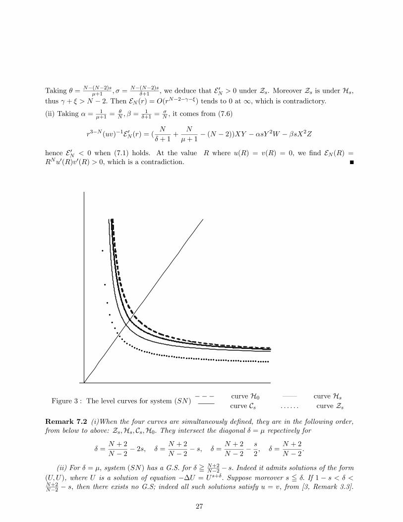
Figure 3 : The level curves for system (SN)−−− curve H0 – – curve Hs– curve Cs . . . . . . curve Zs

Remark 7.2 (i)When the four curves are simultaneously defined, they are in the following order,from below to above: Zs,Hs, Cs,H0. They intersect the diagonal δ = µ repectively for

δ =N + 2

N − 2− 2s, δ =

N + 2

N − 2− s, δ =

N + 2

N − 2− s

2, δ =

N + 2

N − 2.

(ii) For δ = µ, system (SN) has a G.S. for δ = N+2N−2 − s. Indeed it admits solutions of the form

(U,U), where U is a solution of equation −∆U = U s+δ. Suppose moreover s 5 δ. If 1 − s < δ <N+2N−2 − s, then there exists no G.S; indeed all such solutions satisfy u = v, from [3, Remark 3.3].

27

Then the point Ps =(N+2N−2 − s,

N+2N−2 − s

)appears to be the separation point on the diagonal; notice

that Ps ∈ Hs.

Next we prove our main existence result of existence of a G.S. valid without restrictions on s.The main idea is to introduce a new energy function Φ by adding two terms in X2 and Y 2 to theenergy EN defined at (7.3). It is constructed in order that Φ′ does not contain Y and Z. Thenwe consider the set of couples (X,Y ) such that Φ′ has a sign, which is bounded by a cubic curve.When (δ, µ) is above Cs, the cubic curve is exterior to the square

K = [0, N − 2]× [0, N − 2] , (7.8)

and then we can apply Theorem 1.1.

Proof of Theorem 1.5. From Theorem 1.1, if s = N+2N−2 , all the regular solutions are G.S..

Thus we can assume s < N+2N−2 . Let j, k ∈ R be parameters, and

Φ(r) = EN (r) + rN[ks

2

vu′2

u+ j

s

2

uv′2

v

]= rN

[u′v′ + αuµ+1vs + βvδ+1us +

σ

rvu′ +

θ

ruv′ + k

s

2

vu′2

u+ j

s

2

uv′2

v

]= rN−2uvΨ = rN−2−γ−ξ(ZX)ξ/2(WY )γ/2Ψ,

whereΨ(X,Y, Z,W ) = XY + αWY + βZX − σX − θY + k

s

2X2 + j

s

2Y 2.

Then

r3−N (uv)−1Φ′(r) = (σ + θ − (N − 2))XY + (Nα− θ)YW + (Nβ − σ)XZ

− (α(µ+ 1)− 1)XYW − (β(δ + 1)− 1)XY Z + (j − α)sY 2W + (k − β)sX2Z

+ ksX2 [X − (N − 2)] + jsY 2 [Y − (N − 2)] + (N − 2−X − Y )(ks

2X2 + j

s

2Y 2).

We eliminate the terms in Z,W by taking j = α = 1µ+1 , k = β = 1

δ+1 , θ = Nα, σ = Nβ. Then weget the function Φ defined at (1.9). Computing its derivative, we obtain after reduction

B(X,Y ) := −2

sr3−N (uv)−1Φ′(r)

= βX2(N − 2−X) + αY 2(N − 2− Y ) +XY

[βX + αY +

2

s(N − 2−Nα−Nβ)

].

From Proposition 7.1 we can assume that N(α + β) − (N − 2) > 0. We determine the sign ofB on the boundary ∂K of the square K defined at (7.8). We have B(0, Y ) = αY 2(N − 2− Y ) = 0and B(X, 0) = βX2(N − 2 −X) = 0. In particular B(0, 0) = 0. Otherwise B(N − 2, Y ) = YΘ(Y )with

Θ(Y ) = αY [2(N − 2)− Y ] + (N − 2)((N − 2)β +2

s(N − 2−Nα−Nβ).

28

On the interval [0, N − 2] , there holds Θ(Y ) > Θ(0). By hypothesis, (δ, µ) is above Cs, or equiva-lently

(α+ β)N

N − 2− 1 5 s

2min(α, β); (7.9)

consequently B(N − 2, Y ) = 0 and similarly B(X,N − 2) = 0. Then B is nonnegative on ∂K and iszero at (0, 0), (0, N − 2), (N − 2, 0). The curve B(X,Y ) = 0 is a cubic with a double point at (0, 0),which is isolated under the condition (7.9): B(X,Y ) > 0 near (0, 0), except at this point. ThenB(X,Y ) > 0 on the interior of K.

Suppose that there exists a regular solution such that X(T ) = Y (T ) = N − 2 at the same timeT. Indeed up to this time (X,Y ) stays in K, thus the function Φ is decreasing. We have Φ(0) = 0,and at the value R = eT , we find

Φ(R) = RN−2−γ−ξ(N − 2)ξ+γ+2

[αW + βZ

N − 2+ 1− (β + α)(

N

N − 2− s

2)

]then Φ(R) > 0, since min(α, β) < α+ β. Therefore from Theorem 1.1, there exists a G.S.

Remark 7.3 We wonder if the limit curve for existence of G.S. would be Hs, or another curve Lsdefined by

(Ls)1

δ + 1+

1

µ+ 1=

N − 2

N − (N−2)s2

,

which ensures that Φ(R) > 0, and also B(N − 2, N − 2) > 0. This curve cuts the diagonal at the

same point Ps =(N+2N−2 − s,

N+2N−2 − s

)as Hs. Notice that Ls is under Hs.

8 The radial potential system

Here we study the nonnegative radial solutions of system (SP ) :

(SP )

−∆pu = |x|a usvm+1,−∆qv = |x|a us+1vm,

with a = b, δ = m+ 1, µ = s+ 1, and we assume (1.5). System (M) becomes

(MP )

Xt = X

[X − N−p

p−1 + Zp−1

],

Yt = Y[Y − N−q

q−1 + Wq−1

],

Zt = Z [N + a− sX − (m+ 1)Y − Z] ,Wt = W [N + b− (s+ 1)X −mY −W ] .

For this system D, γ and ξ are defined by

D = p(1+m)+q(1+s)−pq, (p−1−s)γ+p+a = (m+1)ξ, (q−1−m)ξ+q+b = (s+1)γ,

thus γ and ξ are linked independtly of s,m by the relation

p(γ + 1) = q(ξ + 1) =pq(m+ s+ 2 + a)

D. (8.1)

29

The system is variational. It admits an energy function, given at (1.13), which can also can beobtained by a direct computation in terms of X,Y, Z,W :

EP (r) = ψ

[ZW − s+ 1

pW ((N − p)− (p− 1)X)− m+ 1

qZ((N − q)− (q − 1)Y )

], (8.2)

where

ψ =rN−2−a |u′|p−1 |v′|q−1

usvm= rN−(γ+1)p

[Xq(s+1)(p−1)Y p(m+1)(q−1)Zp(q−m−1)W q(p−s−1)

]1/D.

Then we find

E ′P (r) = (N + a− (s+ 1)N − pp− (m+ 1)

N − qq

)rN−1+aus+1vm+1.

Thus we define a critical line D as the set of (δ, µ) = (m+ 1, s+ 1) such that

N + a = (m+ 1)N − qq

+ (s+ 1)N − pp

, (8.3)

equivalent to pq(m+ s+ 2 + a) = ND, or N + a = (m+ 1)ξ + (s+ 1)γ, or

(γ, ξ) = (N − pp

,N − qq

)

The subcritical case is given by the set of points under D, equivalently γ > N−pp , ξ > N−q

q or(s+ 1) γ + (m+ 1)ξ > N + a. The supercritical case is the set of points above D.

Remark 8.1 The energy (EP)0 of the particular solution associated to M0 is still negative: (EP )0 =

−Dpq r

N+a−(γ+1)p[Xq(p−1)0 Y

p(q−1)0 Z

q(s+1)0 W

p(m+1)0

]1/D.

Remark 8.2 When p = q = 2, another energy function can be associated to the transformationgiven at Remark 2.2: the system (2.9) relative to u(r) = r−γU(t), v(r) = r−ξV(t) is

Utt + (N − 2− 2γ)Ut − γ(N − 2− γ)U + UsVm+1 = 0Vtt + (N − 2− 2γ)Vt − γ(N − 2− γ)V + Us+1Vm = 0

(8.4)

and the function

EP (t) =s+ 1

2(U2

t − γ(N − 2− γ)U2) +m+ 1

2(V2

t − γ(N − 2− γ)V2 + Us+1Vm+1 (8.5)

satisfies(EP )t = −(N − 2− 2γ)

[(s+ 1)U2

t + (m+ 1)V2t

]It differs from EP , even in the critical case. This point is crucial for Section 9.

30

It has been proved in [34], [35], that in the subcritical case with a = 0, there exists a solution ofthe Dirichlet problem in any bounded regular domain Ω of RN ; and in the supercritical case thereexists no solution if Ω is starshaped. Here we prove two results of existence or nonexistence of G.S.which seem to be new:

Proof of Theorem 1.6. 1) Existence or nonexistence results.

• In the supercritical or critical case there exists a G.S. From Theorem 1.1, if it were not true,then there would exist regular positive solutions of (MP ) such that X(T ) = N−p

p−1 and Y (T ) = N−qq−1 .

It would satify EP 5 0. Then at time T, we find EP (R) > 0, from (8.2), since W > 0, Z > 0, whichis impossible.

• In the subcritical case, there exists no G.S. Suppose that there exists one. Now EP is nonde-creasing, hence EP = 0. Its trajectory stays in the box A defined by (5.1), thus it is bounded. Ifq = m+ 1 and p = s+ 1, we deduce that , EP (r) = O(rN−(γ+1)p) from (8.2), then EP tends to 0 at∞, which is contradictory. Next consider the general case. We have

EP (r) 5 rN−(γ+1)p[Xq(p−1)Y p(q−1)Zp(q−m−1)W q(p−s−1)

]1/DZW

= rN−(γ+1)p[Xq(p−1)Y p(q−1)Zq(1+s)W p(1+m)

]1/D,

then the same result holds. Consequently, from Theorem 1.1, there exists a solution of the Dirichletproblem

2) Behaviour of the G.S. in the critical case.

Let T be the trajectory of a G.S.; then EP (0) = 0, thus T lies on the variety V of energy 0, alsodefined by

qW [(s+ 1)((p− 1)X − (N − p)) + pZ] = p(m+ 1)Z [(N − q)− (q − 1)Y )] (8.6)

and Y < N−qq−1 , hence (s + 1)((p − 1)X − (N − p)) + pZ > 0. From (5.2), T starts from N0 =

(0, 0, N + a,N + b) and stays in A. Eliminating W in system (M), we find a system of threeequations

Xt = X[X − N−p

p−1 + Zp−1

],

Yt = Y F,Zt = Z [N + a− sX − (m+ 1)Y − Z] ,

where

F (X,Y, Z) =1

q

[N − qq − 1

− Y]p(m+ 1− q)Z + q(s+ 1)((N − p)− (p− 1)X)

(s+ 1)((p− 1)X − (N − p)) + pZ.

(i) If T converges to a fixed point of the system in R, the possible points on V are A0, I0, J0, P0,Q0, G0, H0, R0, S0. The eigenvalues of the linearized problem at A0, given by (10.3) satisfy

λ1, λ2 > 0, λ3 = N + a− sN − pp− 1

− (m+ 1)N − qq − 1

5 λ4 = λ∗ = N + a− (s+ 1)N − pp− 1

−mN − qq − 1

,

31

since q 5 p, and λ3 < λ∗ for q 6= p, and λ3 = λ∗ < 0 for q = p, from (8.3). Then A0 can be attainedonly when λ∗ 5 0, from Proposition 4.5. And P0 can be attained only if

q > m+ 1, λ∗ = 0 and q + a < (s+ 1)N − pp− 1

, (8.7)

from Proposition 4.6, because γ = N−pp < N−p

p−1 .We observe that the condition λ∗ = 0 joint to (8.3)

implies m+ 1 < q < p and is equivalent to (8.7). Indeed it implies

N − pp− 1

(s+ 1) 5 N + a−mN − qq − 1

= N + a− q

q − 1(N + a− N − q

q− (s+ 1)

N − pp

);

then

(s+ 1)N − pp− 1

q − pp

5 −(a+ q),

thus q < p. From (8.3) we obtain

(N − q)(m+ 1

q− 1) = q + a− (s+ 1)

N − pp

5 (s+ 1)N − pp

(p− qp− 1

− 1) < 0,

hence m+ 1 < q and (8.7) follows. By symmetry, Q0 cannot be attained since q 5 p. Then A0 andP0 are incompatible, unless A0 = P0, and P0 is not attained when p = q.

(ii) Next we show that T converges to A0 or to P0. If t is an extremum value of Y , then

(m+ 1

q− 1)Z(t) +

s+ 1

p((N − p)− (p− 1)X(t)) = 0. (8.8)

This relation implies q > m+ 1 and

Xt(t) =X(t)Z(t)

p− 1

[1 +

p(m+ 1− q)q(s+ 1)

]=

DX(t)Z(t)

(p− 1)q(s+ 1)> 0.

In the same way, if t is an extremum value of X, then p > s + 1 and Yt(t) > 0. Near −∞, thereholds Xt, Yt = 0, and Zt,Wt 5 0, from the linearization near N0. Suppose that X has a maximumat t0 followed by a minimum at t1. Then p > s + 1, and Y is increasing on [t0, t1]. At time t0 wehave (p − 1)X(t0) + Z(t0) = N − p and Xtt(t0) 5 0, thus Zt(t0) 5 0; eliminating Z we deducep + a + (p − 1 − s)X(t0) 5 (m + 1)Y (t0) and similarly (m + 1)Y (t1) 5 p + a + (p − 1 − s)X(t1);hence Y (t1) < Y (t0), which is a contradiction. Thus X and Y can have at most one maximum, andin turn they have no maximum point. Therefore X and Y are increasing, and they are bounded,

hence X has a limit in(

0, N−pp−1

]and Y has a limit in

(0, N−qq−1

]. Then Z,W are decreasing; indeed

at each time where Zt = 0, we have Ztt = Z(−sXt − (m+ 1)Yt) < 0, thus it is a maximum, whichis impossible.

Then T converges to a fixed point of the system. Moreover, since X and Y are increasing, itcannot be one of the points I0, J0, G0, H0, R0, S0. It is necessarily A0 or P0. We distinguish twocases:

• Case q 5 m+ 1. Then T converges to A0, and λ3, λ∗ < 0, then (1.10) follows.

32

• Case q > m + 1. Then T converges to A0 (resp. P0) when λ∗ 5 0 (resp. λ∗ = 0). If theinequalities are strict, we deduce the convergence of u and v from Propositions 4.5 and 4.6, and(1.11) follows. If λ∗ = 0, then P0 = A0, and λ3 = (N−1)(q−p)

(p−1)(q−1) < 0. The projection of the trajectory

T in R3 on the plane Y = N−qq−1 satisfies the system

Xt = X

[X − N − p

p− 1+

Z

p− 1

], Zt = Z

[N + a− sX − (m+ 1)

N − qq − 1

− Z]

which presents a saddle point at (N−pp−1 , 0), thus the convergence of X and Z is exponential, inparticular we deduce the behaviour of u. The trajectory enters by the central variety of dimension1, and by computation we deduce that Y = N−q

q−1 −1

q−1−m t−1 +O(t−2+ε), then (1.12) follows.

9 The nonradial potential system of Laplacians

Here we study the possibly nonradial solutions of the system of the preceeding Section whenp = q = 2 :

(SL)

−∆u = |x|a usvm+1,−∆v = |x|a us+1vm,

with D = s + m. We solve an open problem of [7]: the nonexistence of (radial or nonradial) G.S.under condition (1.14).

It was shown in [7] in the case N + a = 4. The problem was open when N + a < 4, andm+s+1 > (N +a)/(N −2), which implies N < 6. Indeed in the case m+s+1 5 (N +a)/(N −2),there are no solutions of the exterior problem, see [6, Theorem 5.3]. Recall that the main result of[7] is the obtention of apriori estimates near 0 or ∞, by using the Bernstein technique introducedin [18] and improved in [8]. Then the behaviour of the solutions is obtained by using the change ofunknown

u(r, θ) = r−γU(t, θ), v(r, θ) = r−γV(t, θ), t = ln r,

extending the transformation of Remark 8.2 to the nonradial case (in fact here t is −t in [7]); itleads to the system

Utt + (N − 2− 2γ)Ut + ∆SU− γ(N − 2− γ)U + UsVm+1 = 0,

Vtt + (N − 2− 2γ)Vt + ∆SV − γ(N − 2− γ)V + Us+1Vm = 0,

where ∆S is the Laplace-Beltrami operator on SN−1. A corresponding energy is introduced in [7]:

EL(t) =s+ 1

2

∫SN−1

(U2t − |∇SU|2 − γ(N − 2− γ)U2)dθ

+m+ 1

2

∫SN−1

(V2t − |∇SV|2 − ξ(N − 2− ξ)V2)dθ +

∫SN−1

Us+1Vm+1dθ,

extending (8.5) to the nonradial case; it satisfies

(EL)t = −(N − 2− 2γ)

∫SN−1

[(s+ 1)U2

t + (m+ 1)V2t

]dθ

33

Here we construct another energy function, extending the Pohozaev function defined at (1.13) tothe nonradial case.

Lemma 9.1 Consider the function EL(r) defined by

r−NEL(r) =s+ 1

2

∫SN−1

[u2r − r−2 |∇Su|2 + (N − 2)

uurr

]dθ

+m+ 1

2

∫SN−1

[(∂v

∂ν)2 − r−2 |∇Sv|2 + (N − 2)

vvrr

]dθ + ra

∫SN−1

us+1vm+1dθ.

Then the following relation holds:

r1−NE ′L(r) = (N + a− (s+ 1)N − 2

2− (m+ 1)

N − 2

2)ra

∫SN−1

us+1vm+1dθ.

Proof. In terms of t, we find

EL(t) = EL,1(t) + EL,2(t) + EL,3(t), with

EL,1(t) =s+ 1

2e(N−2)t

∫SN−1

[u2t − |∇Su|

2 + (N − 2)uut

]dθ,

EL,2(t) =m+ 1

2e(N−2)t

∫SN−1

[v2t − |∇Sv|

2 + (N − 2)vvt

]dθ, EL,3(t) = e(N+a)t

∫SN−1

us+1vm+1dθ,

and u satisfies the equations

utt + (N − 2)ut + ∆Su+ e(2+a)tusvm+1 = 0, (9.1)

(e(N−2)tut)t + e(N−2)t∆Su+ e(N+a)tusvm+1 = 0, (9.2)

and v satisfies symmetrical equations. Multiplying (9.2) by u and (9.1) by (s + 1)e(N−2)tut, weobtain

0 =

∫SN−1

u(e(N−2)tut)t + e(N−2)t

∫SN−1

u∆Su+ e(N+a)t

∫SN−1

us+1vm+1

=d

dt

∫SN−1

ue(N−2)tut − e(N−2)t

∫SN−1

(u2t + |∇Su|2) + e(N+a)t

∫SN−1

us+1vm+1

d

dt

∫SN−1

s+ 1

2(N − 2)ue(N−2)tut −

s+ 1

2(N − 2)e(N−2)t

∫SN−1

(u2t + |∇Su|2)

= −s+ 1

2(N − 2)e(N+a)t

∫SN−1

us+1vm+1,

34

and symmetrically for v, and adding the equalities we deduce

0 = (s+ 1)(e(N−2)t d

dt

∫SN−1

(u2t − |∇Su|

2

2+ (N − 2)e(N−2)t

∫SN−1

u2t

+ (m+ 1)(e(N−2)t d

dt

∫SN−1

v2t − |∇Sv|

2

2+ (N − 2)e(N−2)t

∫SN−1

v2t

+d

dt(e(N+a)t

∫SN−1

us+1vm+1)− (N + a)e(N+a)t

∫SN−1

us+1vm+1

d

dt

e(N−2)t

2

∫SN−1

((s+ 1)(u2t − |∇Su|

2) + (m+ 1)(v2t − |∇Sv|

2)) + e(N+a)t

∫SN−1

us+1vm+1

+N − 2

2e(N−2)t

∫SN−1

((s+ 1)(u2t + |∇Su|2) + (m+ 1)(v2

t + |∇Sv|2))

= (N + a)e(N+a)t

∫SN−1

us+1vm+1,

hence

(EL)t(t) = (N + a− (s+ 1)N − 2

2− (m+ 1)

N − 2

2)e(N+a)t

∫SN−1

us+1vm+1dθ.

Proof of Theorem 1.7. Suppose that there exists a G.S. Since s+m+1 < (N+2+2a)/(N−2)we deduce that EL and EL are increasing and start from 0, then they stay positive. From [7,Corollary 6.4], since s+m+1 < (N +2)/(N −2), three eventualities can hold. The first one is that(u, v) behaves like the particular solution (u0, v0); it cannot hold because EL has a negative limit,see [7, Remark 6.3]. The second one is that (u, v) is regular at ∞, that means lim|x|→∞ |x|N−2 u =

α > 0, lim|x|→∞ |x|N−2 v = β > 0; it cannot hold because limt→∞EL(t) = 0. It remains a thirdeventuality: when for example m > (N + a)/(N − 2), and (u, v) has the following behaviour at ∞ :

limr→∞

u = α > 0, and lim|x|→∞

|x|k v = β > 0 or 0, with k = (2 + a)/(m− 1). (9.3)

The condition onm implies that N < 4−a from assumption (1.14). In that case limt→∞EL(t) =∞,which gives no contradiction. Here we show that a contradiction holds by using the new energyfunction EL.

First recall the proof of (9.3). Making the substitution

u(r, θ) = u(t, θ), v(r, θ) = r−kV(t, θ), t = ln r, θ ∈ SN−1,

we get utt + (N − 2)ut + ∆Su +e−2ktusVm+1 = 0,

Vtt + (N − 2− 2k)Vt + ∆SV − k(N − 2− k)V+us+1Vm = 0.(9.4)

35

Then u,V are bounded near ∞, and from [7, Proposition 4.1] u converges exponentially to theconstant α, more precisely

‖|u−α|+ |ut|+ |∇Su|‖C0(SN−1) = O(e−(N−2)t), (9.5)

because k 6= (N − 2)/2 and all the derivatives of V up to the order 2 are bounded. The equationin V takes the form

Vtt + (N − 2− 2k)Vt + ∆SV − k(N − 2− k)V+αs+1Vm + ϕ = 0

where ϕ and its derivatives up to the order 2 are O(e−(N−2)t). From [7, Theorem 4.1], the functionV converges to β or to 0 in C2(SN−1).

Next we define

f(t) = e(N−2)t

∫SN−1

utdθ = rN−1

∫SN−1

urdθ.

ThenEL,1(t) = (N − 2)

s+ 1

2αf(t) +O((e−(N−2)t))

from (9.5). Moreover from (9.4),

ft(t) = −e(N−2−2k)t

∫SN−1

usVm+1dθ < 0.

Since u is regular at 0, f(t) = 0(e(N−1)t) at −∞, in particular limt→−∞ f(t) = 0. And ft(t) =O(e(N−2−2k)t) = O(e−t) at ∞, then f(t) has a finite negative limit −`2; and

limt→∞EL,1(t) = −(N − 2)

s+ 1

2α`2.

Moreover v = e−ktV, and V and its derivatives up to the order 2 are bounded, thus

EL,2(t) = O(e(N−2−2k)t) = O(e−t)

FinallyEL,3(t) = O(e(N+a−k(m+1))t)

and N + a− k(m+ 1) < 2−Nm−1 < 0. Then EL has a finite limit θ < 0 at ∞, which is contradictory.

10 Analysis of the fixed points

Here we make the local analysis around the fixed points.

Proof of Proposition 4.4. (i) Consider a regular solution (u, v) with initial data (u0, v0).When when r → 0, we have

(−rN−1∣∣u′∣∣p−2

u′)′ = rN−1+aus0vδ0(1 + o(1)), −

∣∣u′∣∣p−2u′ =

1

N + ar1+aus0v

δ0(1 + o(1)),

36

thus from (2.1), when t→ −∞

X(t) = (1

N + aus+1−p

0 vδ0)1/(p−1)e(p+a)t/(p−1)(1 + o(1)),

Y (t) = (1

N + buµ0v

m+1−q0 )1/(q−1)e(q+b)t/(q−1)(1 + o(1)),

and limt→−∞ Z = N + a, limt→−∞W = (N + b). In particular the trajectory tends to N0 =(0, 0, N + a,N + b).

(ii) Reciprocally, consider a trajectory converging to N0. Setting Z = N + a+ Z,W = N + b+ W ,the linearized system is

Xt =p+ a

p− 1X, Yt =

q + b

q − 1Y, Zt = (N+a)

[−sX − δY − Z

], Wt = (N+b)

[−µX −mY − W

].

(10.1)The eigenvalues are

λ1 =p+ a

p− 1> 0, λ2 =

q + b

q − 1> 0, λ3 = −(N + a) < 0, λ4 = −(N + b) < 0. (10.2)

The unstable variety Vu and the stable variety Vs have dimension 2. Notice that Vs is containedin the set X = Y = 0, thus no admissible trajectory converges to N0 when r → ∞, and thereexists an infinity of admissible trajectories in R, converging to N0 when r → 0. Moreover we getlimt→−∞ e−(p+a)/(p−1)tX(t) = κ > 0 and limt→−∞ e−(q+b)/(q−1)tY (t) = ` > 0. Thus (u, v) have apositive limit (u0, v0) = ((N + a)κp−1)(q−1−m)/D((N + b)`q−1)δ/D from (4.2), (4.1), hence (u, v) isa regular solution.

Next we show that for any κ > 0, ` > 0 there exists a unique local solution such thatlimt→−∞ e−(p+a)t/(p−1)X(t) = κ and limt→−∞ e−(q+b)/(q−1)tY = `. On Vu, we get a system oftwo equations of the form

Xt = X(λ1 + F (X,Y )), Yt = Y (λ2 +G(X,Y )),

where F = AX + BY + f(X,Y ), where f is a smooth function with fX(0, 0) = fY (0, 0) = 0,similarly for G. Setting X = eλ1t(κ + x), Y = eλ2t(` + y), and assuming λ2 = λ1 and settingρ = eλ1t we obtain

xρ =1

ρ(κ+ x)F (ρ(κ+ x), ρλ2/λ1(`+ y)), yρ = (`+ y)G(ρ(κ+ x), ρλ2/λ1(`+ y)),

with x(0) = y(0) = 0. Then we get local existence and uniqueness. Hence for any u0, v0 > 0 thereexists a regular solution (u, v) with initial data (u0, v0). Moreover u, v ∈ C1([0, R)) when a, b > −1.

Proof of Proposition 4.5. The linearization at A0 =(N−pp−1 ,

N−qq−1 , 0, 0

)gives, with X =

N−pp−1 + X, Y = N−q

q−1 + Y ,

Xt =N − pp− 1

[X +

Z

p− 1

], Yt =

N − qq − 1

[Y +

W

q − 1

], Zt = λ3Z, Wt = λ4W.

37

The eigenvalues are

λ1 =N − pp− 1

> 0, λ2 =N − qq − 1

> 0, λ3 = N+a−sN − pp− 1

−δN − qq − 1

, λ4 = N+b−µN − pp− 1

−mN − qq − 1

.

(10.3)• Convergence when r →∞ : If λ3 > 0, or λ4 > 0, then the stable varietyVs has at most dimension 1,it satisfiesW = 0 or Z = 0, hence there is no admissible trajectory converging to A0 at∞. If λ3 < 0,and λ4 < 0, then Vs has dimension 2. Moreover Vs ∩ Z = 0 has dimension 1 : the correspondingsystem in X,Y,W has the eigenvalues λ1, λ2, λ4; similarly Vs ∩ W = 0 has dimension 1. Thenthere exist trajectories in Vs such that Z > 0 and W > 0, included in R and thus admissible. Theysatisfy lim e−λ3tZ = C3 > 0, lim e−λ4tW = C4 > 0, then (4.11) follows from (4.2).

• Convergence when r → 0 : If λ3 < 0, or λ4 < 0, the unstable variety Vu has at most dimension3, and it satisfies W = 0 or Z = 0. Therefore there is no admissible trajectory converging at −∞.If λ3, λ4 > 0, then Vu has dimension 4; in that case there exist admissible trajectories, and (4.11)follows as above.

Proof of Proposition 4.6. We set P0 =(N−pp−1 , Y∗, 0,W∗

), with

Y∗ =

N−pp−1 µ− (q + b)

q − 1−m , W∗ =(q − 1)(N + b− N−p

p−1 µ)−m(N − q)q − 1−m ,

for m+ 1 6= q. The linearization at P0 gives, with X = N−pp−1 + X, Y = Y∗ + Y , W = W∗ + W ,

Xt =N − pp− 1

[X +

Z

p− 1

], Yt = Y∗

[Y +

W

q − 1

], Zt = λ3Z, Wt = W∗

[−µX −mY − W

]The eigenvalues are

λ1 =N − pp− 1

> 0, λ3 = N + a− sN − pp− 1

− δY∗ =D

q − 1−m(γ − N − pp− 1

),

and the roots λ2, λ4 of equation

λ2 − (Y∗ −W∗)λ+m+ 1− qq − 1

Y∗W∗ = 0

Then if λ3 < 0 (resp. λ3 > 0) there is no admissible trajectory converging when r → 0 (resp.r →∞). Indeed Vu = Vu ∩ Z = 0 (resp. Vs = Vs ∩ Z = 0).

1) Suppose that q > m + 1. Since q + b < N−pp−1 µ < N + b − mN−q

q−1 , we have P0 ∈ R, andλ2λ4 < 0. First assume λ3 < 0, that means γ < N−p

p−1 . Then Vs has dimension 2, and Vs ∩ Z = 0has dimension 1, there exists trajectories with Z > 0, which are admissible, converging whenr →∞. Next assume λ3 > 0. Then Vu has dimension 3, and Vu ∩ Z = 0 has dimension 2. Thusthere exist admissible trajectories converging when t→ −∞.

2) Suppose that q < m+1. Since q+b > N−pp−1 µ > N+b−mN−q

q−1 , we have P0 ∈ R, and λ2λ4 > 0.

We assume qN−pp−1 µ+m(N − q) 6= N(q − 1) + (b+ 1)q, that means Y∗ 6= W∗. First suppose λ3 > 0,

that means γ < N−pp−1 . If Reλ2 > 0, then Vu has dimension 4, or Reλ2 < 0 then Vu has dimension

38

2 and Vu ∩ Z = 0 has dimension 1. In any case, there exist admissible trajectories convergingwhen r → 0. Next assume λ3 < 0. If Reλ2 > 0, then Vs has dimension 1, and Vs ∩ Z = 0 = ∅.If Reλ2 < 0, then Vs has dimension 3. In any case Vs contains trajectories with Z > 0, which areadmissible, converging when r →∞.

Those trajectories satisfy lim e−λ3tZ = C3 > 0, limX = N−pp−1 , limY = Y∗ and limW = W∗,

thus (4.12) follows from (4.2) and (2.5).

Proof of Proposition 4.8. The linearization at I0 = (N−pp−1 , 0, 0, 0) gives, with X = N−pp−1 + X,

Xt =N − pp− 1

(X+Z

p− 1), Yt = −N − q

q − 1Y, Zt = (N+a−sN − p

p− 1)Z, Wt = (N+b−µN − p

p− 1)W.

The eigenvalues are

λ1 =N − pp− 1

> 0, λ2 = −N − qq − 1

< 0, λ3 = N + a− sN − pp− 1

, λ4 = N + b− µN − pp− 1

.

• Convergence when r → ∞ : If λ3 > 0 or λ4 > 0, then Vs = Vs ∩ Z = 0 or Vs = Vs ∩ W = 0.There is no admissible trajectory converging at ∞. Next suppose that λ3, λ4 < 0. Then Vs hasdimension 3; it contains trajectories with Y,Z,W > 0, which are admissible. They satisfy limX =N−pp−1 , lim e−λ2tY = C2 > 0, lim e−λ3tZ = C3 > 0, lim e−λ4tW = C4 > 0, then (4.13) follows from(4.2) and (2.4).

• Convergence when r → 0 : Since λ2 < 0 we have Vu = Vu∩Y = 0 , hence there is no admissibletrajectory converging when r → 0.

Proof of Proposition 4.9. The point G0 = (N−pp−1 , 0, 0, N+b−N−pp−1 µ) ∈ R since N−pp−1 µ < N+b.

The linearization at G0 gives, with X = N−pp−1 + X,W = N + b− N−p

p−1 µ+ W ,

Xt =N − pp− 1

[X +

Z

p− 1

], Yt =

Y

q − 1(q + b− N − p

p− 1µ),

Zt = (N + a− sN − pp− 1

)Z, Wt = (N + b− N − pp− 1

µ)[−µX −mY − W

]The eigenvalues are

λ1 =N − pp− 1

> 0, λ2 =1

q − 1(q + b− N − p

p− 1µ), λ3 = N + a− sN − p

p− 1, λ4 =

N − pp− 1

µ−N − b < 0.

• Convergence when r → ∞ : If λ2 > 0, or λ3 > 0, then Vs = Vs ∩ Y = 0 or Vs = Vs ∩ Z = 0,there is no admissible trajectory converging at ∞. Assume λ2, λ3 < 0, then Vs has dimension 3, itcontains trajectories with Y,Z > 0, which are admissible.

• Convergence when r → 0 : If λ3 < 0, or λ2 < 0 there is no admissible trajectory. If λ2, λ3 > 0then Vs has dimension 3, it contains admissible trajectories.

In any case limX = N−pp−1 , lim e−λ2tY = C2 > 0, lim e−λ3tZ = C3 > 0, limW = N + b− N−p

p−1 µ,hence (4.13) still follows from (4.2) and (2.4).

Proof of Proposition 4.10. We set C0 =(0, Y , 0, W

), with

Y =q + b

m+ 1− q , W =m(N − q)− (N + b)(q − 1)

m+ 1− q . (10.4)

39

Then C0 ∈ R if N−qq−1 m > N + b, implying q < m+1. The linearization at C0 gives, with Y = Y + Y

and W = W + W

Xt = −N − pp− 1

X, Yt = Y

[Y +

W

q − 1

], Zt = λ3Z, Wt = W

[−µX −mY − W

].

The eigenvalues are

λ1 = −N − pp− 1

, λ3 = N + a− δY ,

and the roots λ2, λ4 of equation

λ2 − (Y − W )λ+m+ 1− qq − 1

Y W = 0 (10.5)

then λ2λ4 > 0. We assume m 6= N(q−1)+(b+1)qN−q , that means Y 6= W .

• Convergence when r → ∞ : if λ3 > 0 we have Vs = Vs ∩ Z = 0 , hence there is no admissibletrajectory. Next assume that λ3 < 0, that means δ > (N + a)m+1−q

q+b .If Reλ2 < 0 (resp. > 0) thenVs has dimension 4 (resp. 2) and Vs ∩ X = 0 and Vs ∩ Z = 0 have dimension 3 (resp. 1) thenthere exist trajectories with X,Z > 0, which are admissible.

In any case lim e−λ1tX = C1 > 0, limY = Y , lim e−λ3tZ = C3 > 0, limW = W , then (4.15)follows.

• Convergence when r → 0 : Since λ1 < 0 we have Vu = Vu∩X = 0 , hence there is no admissibletrajectory.

Proof of Proposition 4.11. We set R0 =(0, Y , Z, W

), where Y , W are defined at (10.4), and

Z = N+a−δ b+qm+1−q .Under our assumptions it lies inR. Setting Y = Y +Y , Z = Z+Z,W = W+W ,

the linearization at R0 gives

Xt = λ1X, Yt = Y

[Y +

W

q − 1

], Zt = Z

[−sX − δY − Z

], Wt = W

[−µX −mY − W

];

the eigenvalues are

λ1 =1

p− 1(p+ a− δ b+ q

m+ 1− q ), λ3 = −Z < 0;

and the roots λ2, λ4 of equation of equation (10.5).

• Convergence when r → ∞ : If λ1 > 0, that means (p + a)m+1−qq+b < δ, then Vs = Vs ∩ X = 0 ,

hence there is no admissible trajectory. Next assume λ1 < 0; if Reλ2 < 0 (resp. > 0) then Vshas dimension 4(resp. 2) and Vs ∩ X = 0 has dimension 3 (resp. 1) then there exist admissibletrajectories.

• Convergence when r → 0 : If λ1 < 0, then Vu = Vu ∩ X = 0 , hence there is no admissibletrajectory. Next assume λ1 > 0. If Reλ2 = Reλ4 < 0 (resp. > 0) then Vs has dimension 4 (resp.2) and Vs ∩ X = 0 has dimension 3 (resp. 1) then there exist admissible trajectories.

In any case lim e−λ1tX = C1 > 0, limY = Y , limZ = Z, limW = W , then (4.15) holds again.

40

Remark 10.1 Finally there is no admissible trajectory converging to 0 = (0, 0, 0, 0), or K0 =(0, 0, N + a, 0), or L0 = (0, 0, 0, N + b). Indeed the linearization at 0 gives

Xt = −N − pp− 1

X, Yt = −N − qq − 1

Y, Zt = (N + a)Z, Wt = (N + b)W

Then Vs and Vu have dimension 2, hence Vs is contained in Z = W = 0 , and Vu in X = Y = 0 .The linearization at K0 gives, with Z = N + a+ Z,

Xt =p+ a

p− 1X, Yt = −N − q

q − 1Y, Zt = (N + a)

[−sX − δY − Z

], Wt = (N + b)W.

The eigenvalues are p+ap−1 ,−

N−qq−1 ,−(N + a), N + b. Then Vs and Vu have dimension 2, hence Vs is

contained in Z = W = 0, and Vu in Y = 0 . The case of L0 follows by symmetry.

References

[1] Azizier C., Clément P. and Mitidieri E., Existence and a Priori Estimates for Positive Solutionsof p-Laplace Systems, Journal of Differential Equations 184 (2002), 422—442.

[2] Bidaut-Véron M.F., Local and global behavior of solutions of quasilinear equations of Emden-Fowler type, Arc. Rat. Mech. and Anal., 107 (1989), 293-324.

[3] Bidaut-Véron M.F., Local behaviour of solutions of a class of nonlinear elliptic systems, Adv.in Diff. Equ. 5 (2000), 147-192.

[4] Bidaut-Véron M.F. and Grillot P., Singularities in Elliptic systems with absorption terms,Ann. Scuola Norm. Sup. Pisa, 28 (1999), 229-271.

[5] Bidaut-Véron M.F. and Grillot P., Asymptotic behaviour of elliptic systems with mixed absorp-tion and source terms, Asymtotic Anal., 19 (1999), 117-147.

[6] Bidaut-Véron M.F. and Pohozaev S., Nonexistence results and estimates for some nonlinearelliptic problems, J. Anal. Mathématique, 84 (2001), 1-49.

[7] Bidaut-Véron M.F. and Raoux T., Asymptotics of solutions of some nonlinear elliptic systems,Comm. Part. Diff. Equ., 21 (1996), 1035-1086.

[8] Bidaut-Véron M.F. and Véron L., Nonlinear elliptic equations on compact Riemannian mani-folds and asymptotics of Emden equations, Invent. Math. 106 (1991), 489-539.

[9] Busca J. and Manasevitch R., A Liouville-type theorem for Emden system, Indiana Univ. Math.J. 51 (2002), 37-51.

[10] Chen S. and Lu G., Existence and nonexistence of positive radial solutions for a class ofsemilinear elliptic system, Nonlinear Analysis 38 (1999) 919-932.

[11] Chicone C. and Tian J., On general properties of quadratic systems, Proc. Amer. Math. Soc.89 (1982), 167—178.

41

[12] Clément P., Fleckinger J., Mitidieri E. and de Thélin F., Existence of positive solutions for anonvariational quasilinear elliptic system, J. Differential Equations 166 (2000), 455—477.

[13] Clément P., Garcia-Huidobro M., Guerra I. and Manasevich R., On regions of existence andnonexistence for a system of p-q Laplacians, Asymptot. Anal. 48 (2006), 1—18.

[14] de Figueiredo D., Peral I. and Rossi J., The critical hyperbola for a Hamiltonian elliptic systemwith weights, Annali di Matematica 187(2008), 531—545.

[15] de Figueiredo D. and Felmer P., A Liouville type theorem for elliptic systems, Ann. ScuolaNorm. Sup. Pisa Cl. Sci. 2& (1994), 387-397.

[16] Fowler R.H., Further studies of Emden’s and similar differential equations, Quart. J. Math 2(1931), 259-288.

[17] Garcia M., Manasevitch R., Mitidieri E., and Yarur C., Existence and nonexistence of singularpositive solutions for a class of semilinear elliptic systems, Arch. Rat. Mech. Anal. 140 (1997),253-284.

[18] Gidas B. and Spruck J., Global and local behavior of positive solutions of nonlinear ellipticequations, Comm. Pure Appl. Math. 34 (1981), 525—598.

[19] Guedda M. and Véron L, Local and global properties of solutions of nonlinear elliptic equations,J. Diff. Equ., 76 (1988), 159—189.

[20] Hülshof J. and vander Vorst R., Asymptotic behaviour of ground states, Proc. Amer. Math.Soc. 124 (1996), 2423-2431.

[21] Lin C.S., A classification of solutions of a conformally invariant fourth order equation in RN ,Comment. Math. Helv. 73 (1998), 206—231.

[22] Lions P.L., The concentration-compactness principle in the calculus of variations, part 1, Rev.Mat. Iberoam. 1 (1985), 145-201.

[23] Liu F. and Yang J., Nontrivial solutions of Hardy-Henon type elliptic systems, preprint.

[24] Lu Q. and Yang Z, Blow-up estimates for a quasi-linear reaction—diffusion system, Math. Meth.Appl. Sci. 26 (2003), 1005—1023.

[25] Mitidieri E., A Rellich type identity and applications, Comm. P.D.E. 18 (1993), no. 1-2, 125—151.

[26] Mitidieri E., Nonexistence of positive solutions of semilinear elliptic systems in RN , Diff. Int.Equ. 9 (1996), 465-479.

[27] Raoux T., Thèse de Doctorat, Université de Tours (1995).

[28] Reichel W. and Zou H., Nonexistence results for semilinear cooperative systems via movingspheres, J. Diff. Equ., 161 (2000), 219-243.

[29] Serrin J. and Zou H., Existence of positive solutions of the Lane-Emden system, Atti Sem.Mat. Fis. Univ. Modena, 46 (1998), suppl., 369-380.

42

[30] Serrin J. and Zou H., Existence of positive entire solutions of elliptic Hamiltonian systems,Comm. Partial Differential Equations 23 (1998), 577—599.

[31] Serrin J. and Zou H., Non-existence of positive solutions of Lane-Emden systems, Diff. Int.Equ., 9 (1996), 635-653.

[32] Serrin J. and Zou H., Non-existence of positive solutions of semilinear elliptic systems, Atribute to Ilya Bakelman (College Station, TX, 1993), 55—68, Discourses Math. Appl., 3, TexasA & M Univ., College Station, TX, 1994.

[33] Souplet P., The proof of the Lane-Emden conjecture in 4 space dimensions, Adv. Math. 221(2009), 1409—1427.

[34] De Thélin F. and Vélin J., Existence et non-existence de solutions non triviales pour dessystèmes elliptiques non linéaires, C.R. Acad. Sci. Paris 313 (1991), 589 592.

[35] De Thélin F. and Vélin J., Existence and nonexistence of nontrivial solutions for some non-linear elliptic systems, Rev. Mat. Univ. Comput. Madrid 6 (1993), 153 194.

[36] vanderVorst R., Variational identities and applications to differential systems, Arch. Rat.Mech. Anal. 116 (1991), 375-398.

[37] Véron L., Singularities of solutions of second order quasilinear equations, Pitman ResearchNotes in Math., Longman (1995).

[38] Zheng S., Nonexistence of positive solutions to a semilinear elliptic system and blow-up esti-mates for a reaction—diffusion system, J. Math. Anal. Applic. 232 (1999), 293—311.

[39] Zou H., A priori estimates and existence on strongly coupled cooperative elliptic systems, Glasg.Math. J. 48 (2006), 437-457.

[40] Zou H., A priori estimates and existence for strongly coupled cooperative elliptic systems,Comm. Part. Diff. Equ. 31 (2006), 735-773

[41] Zou H., A note on non-existence results for semi-linear cooperative elliptic systems via movingspheres, Proc. Amer. Math. Soc. 134 (2006), 1635-1646.

[42] Zou H., Existence and non-existence for strongly coupled quasi-linear cooperative elliptic sys-tems, J. Math. Soc. Japan 59 (2007), 393-421.

43