156

TECHNISCHE MECHANIK, 31, 2, (2011), 156 - 170 submitted: March 7, 2011

A Multi-Scale Homogenization Technique Applied to the Elastic Properties of Solders A. Brandmair, W. Müller, M. Savenkova, S. Sheshenin

In modern microelectronic systems solder materials are frequently used. Consequently, it is of great importance to predict their lifetime and stability. In order to perform such an analysis, material properties are required. Since electronic devices and therefore the amounts of used materials become smaller and smaller, the influence of a changing microstructure on the mechanical properties must be examined. First, some analytical methods will be presented leading to upper and lower bounds for standard solder alloys. They also allow for an examina-tion of the influence of certain micro-geometries. Second, a multi-scale approach is used in order to perform a more general analysis of different micro-structures. The constitutive equations are stated and a homogenization technique for elastic properties of arbitrary structures is derived. The resulting equations are solved numerically and the results are presented. For lamellar-type of structures, closed-form formulas are derived and the results will be compared to the numerical ones. 1 Introduction In microelectronic applications solder alloys fulfill an important role. On the one hand side they guarantee the mechanical connection between, e.g., the chip and a printed circuit board. On the other hand side they also estab-lish electrical contact between the components. Therefore the stability of the applied solder-materials is of par-ticular interest for the lifetime-prediction of microelectronic devices. All of the solder alloys that are used show some kind of micro-structural change during aging. For example, the microstructure of an eutectic AgCu28-solder changes over time due to phase-separation followed by coarsening. This is shown in Figure 1.

Figure 1. Coarsening of an AgCu28 structure after 2h, 20h and 40h The development of this particular microstructure is based on the tendency of the solder system to minimize its internal surface. It can be described by using an extended diffusion equation and has been examined in-depth in [1]. As the amount of used solder-material is in general very small, changes in the microstructure cannot be ne-glected when predicting the reliability of such structures. Due to this reason it is important to take the different length-scales into account. In particular it is of interest to examine how the changing microstructure influences the macroscopic material-properties. A direct calculation, e.g., by FE-simulations, is based on rather complex FE-meshes and time-consuming. For this reason a method by means of which reliable results for the material properties can be obtained without having to model the exact structure seems rather useful. In this context, the procedure of homogenizing material properties has shown to be quite promising. The obtained homogenized, effective properties should be able to reproduce the real behaviour of the material to a great extent and would enable us to perform continuum-based FE-simulations of microelectronic devices in order to predict their lifetime and stability without a detailed discretization of the complete micro-structure.

157

2 Boundary Estimates for the Mechanical Properties of Selected Solder-Materials For the examination of boundaries for the mechanical properties of solder-materials two binary solders, namely silver-copper (AgCu), tin-lead (SnPb) and tin-silver (SnAg), were chosen. Furthermore only elastic properties will be investigated and analyzed by means of homogenization. We start by deriving YOUNG’s modulus from the values of the polycrystalline stiffness-tensor ijklC for copper. This serves as an example in order to validate re-sults for the elastic constants which were obtained by using the Embedded-Atom-Method (EAM), which in turn is based on inter-atomic potentials [2]. Figure 2a shows the results for the stiffness-tensor of a single crystal made of copper. The values in brackets show results obtained from the literature for comparison. Based on these val-ues, a direction-dependent compliance '

11S has been calculated by using the following formula where S is the inverse of the stiffness-tensor [3]. Note that this formula only holds for cubic crystal symmetry:

+

++−−−=

22

2222

44121111'11

))cos())cos()(sin(

))cos())sin()(sin())sin()(sin())cos()(sin()

21(2

υϕυ

υϕυϕυϕυSSSSS . (1)

The angles υ and ϕ in (1) are the inclination and the azimuth of a respective spherical coordinate system. In

Figure 2b '11S , the first entry of the direction-dependent compliance tensor, is plotted. 1x - 3x in Figure 2b are the

main crystallographic axes of the cubic copper. In Figure 2c the results for YOUNG’s modulus via averaging over the unit sphere are presented. Young’s modulus was calculated forming the reciprocal of the mean value of '

11S . This transformation of anisotropic material-parameters has been used to validate the elastic-isotropic parameters, used for homogenization.

(a) (b) (c) Figure 2. (a) Stiffness-tensor for copper via EAM (values from literature in brackets), (b) Direction-dependence of the compliance-tensor of copper, (c) YOUNG’s modulus for copper The parameters shown in Table 1 were then used in order to obtain first estimates for the bulk modulus k and for the shear modulus µ of the alloys that were just mentioned. Intuitively speaking, the different phases are con-nected in parallel or in series, and these leads to lower and upper bounds, respectively, which are also known as VOIGT and REUSS limits. The exact geometric form of the ”inclusions,” and therefore the exact form of the mi-crostructure of the alloy, is not taken into account this way and just the volume fractions, ic , need to be known:

∑∑ =

=

≤≤N

iiiN

iii

kckk/c 1

1

1 , ∑∑ =

=

≤≤N

iiiN

iii

c/c 1

1

1µµ

µ. (2)

158

type of metal

YOUNG’s modulus (polycrystal)

YOUNG’s mod-ulus from Cijkl (averaged over unit sphere)

Poisson’s ra-tio, ν

shear modulus, µ , predicted

bulk modulus, k, predicted

Silver Ag 83 GPa 81/65 GPa 0,37 30 GPa 106 GPa

Copper Cu 130 GPa 129/102 GPa 0,34 49 GPa 135 GPa

Tin Sn 50 GPa 40 GPa 0,36 18 GPa 60 GPa

Lead Pb 16 GPa 18 GPa 0,44 5.5 GPa 44 GPa

Table 1. Elastic properties of relevant metals Another analytical approach that leads to upper and lower bounds for the elastic parameters was presented in [4] by HASHIN and SHTRIKMAN. Variational principles in the linear theory of elasticity have been applied to obtain bounds for the effective elastic moduli of arbitrary phase geometry. The resulting formulae for upper and lower bounds of binary structures following this method read:

22

2

21

12

11

1

12

21

4331

4331

µµ ++

−

+≤≤

++

−

+

kc

kk

ckk

kc

kk

ck , (3)

)()(

)()(

222

222

21

12

111

111

12

21

435261

435261

µµµ

µµ

µµ

µµµ

µµ

µ

++

+−

+≤≤

++

+−

+

kck

c

kck

c .

The results for both VOIGT-REUSS and HASHIN-SHTRIKMAN bounds are presented in Table 2. Note that the num-ber in the first column shows the composition of the solder and therefore mass concentrations n have to be con-verted into volume fractions, c, depending on the mass density ρ of the two components as follows:

+

=1

1

21

121

ρρ

nn

c . (4)

Solder alloy Microstructure VOIGT-REUSS bounds HASHIN-SHTRIKMAN bounds

Ag71/Cu29

114,4 < khom[GPa] < 115,8 34,5 < µ hom[GPa] < 36,2

114,7< khom[GPa] < 114,8 34,2 < µ hom[GPa] < 35,4

Sn62/Pb38

54,3 < khom[GPa] < 55,2 11,1 < µ hom[GPa] < 14,7

54,4 < khom[GPa] < 54,6 12,7 < µ hom[GPa] < 13,6

Sn96,5/Ag3,5

60,18 < khom[GPa] < 60,68 18,56 < µ hom[GPa] < 18,68

60,27 < khom[GPa] < 60,32 18,61 < µ hom[GPa] < 18,62

Table 2. Results for upper and lower bounds of elastic properties Obviously the results of both homogenization techniques do not differ significantly. Moreover, the bounds are very close together. Therefore we conclude that not taking the distribution of the specimens in the microstructure

159

into account is very simplistic and a more sophisticated technique should be considered that acknowledges the internal geometry of the microstructure as well. A first approach of this kind is given by using a laminate formulae for a SnPb-structure. This seems particularly suitable for coarsened SnPb solders which show lamella-type of structures, such as the ones shown in Figure 5. These develop after a certain time due to the different crystallographic symmetries of tin and lead. In [5] the following equation for YOUNG’s modulus in the direction of the lamellae is presented. The index l denotes the properties of the lamella and the index m denotes the properties of the matrix. ν denotes the corresponding Pois-son’s ratios:

( )[ ] ( )[ ] 133

4 2

11++++

−++=

////)(

mmffllmm

mmlmlmmll

kckcccEcEcE

µµµµ

µνν. (5)

By using the values given above we obtain 44011 .=E GPa. In order to compare this result with the homogenized properties determined before, we have to calculate YOUNG’s-modulus from the VOIGT-REUSS-bounds of SnPb in Table 2. Since the difference between the POISSON’s ratios of both specimens is not that large, we simply conduct a volumetric averaging and obtain

39.0SnPb =ν . Now by using the relation between YOUNGS’s modulus and the shear-modulus (average value 9.12=µ GPa):

ν)μ(E += 12 (6) we find the a homogenized YOUNG’s modulus of 9.35=E GPa for SnPb, without taking geometric effects into account. Note that by accounting for the geometric effects of a lamellar structure, YOUNG’s modulus has in-creased by roughly 15%. 3 Effective Elastic Moduli of Heterogeneous Materials In the previous section formulae for simple geometries or even without geometrical effects have been used. Now an approach will be presented, which is suitable for a general treatment. We consider a loading range so that an elastic response can be assumed. Consequently, HOOKE’s law holds: ( ) εCσ :x= , (7) where σ and ε denote the stress and strain tensors, respectively. ( )xC is the forth-order elastic moduli tensor, which depends on the local position, x , due to the heterogeneity of the material. The effective elastic moduli, effC , relate the mean (average) stresses and strains through the following relation, which can be found in various publications [6,7,10]: εCσ :eff= (8) where:

( ) VV V

d1∫= xσσ , ( ) V

V V

d1∫= xεε (9)

are the mean stresses and strains, averaged w.r.t. a Representative Volume Element (RVE). Obviously mean values should be independent of the chosen domain V provided V is greater or equal than the defined RVE, and so are effective elastic moduli. By L and l we denote the typical size of the composite material and of the RVE, respectively. The latter contains various material inclusions of size δ (Figure 3). In the case of an alloy the RVE consist of several phases. The

160

defined sizes are assumed to be related by the inequality δ < l << L. Keeping this in mind we introduce a small-scale parameter, ε, by the equation:

Ll

=ε . (10)

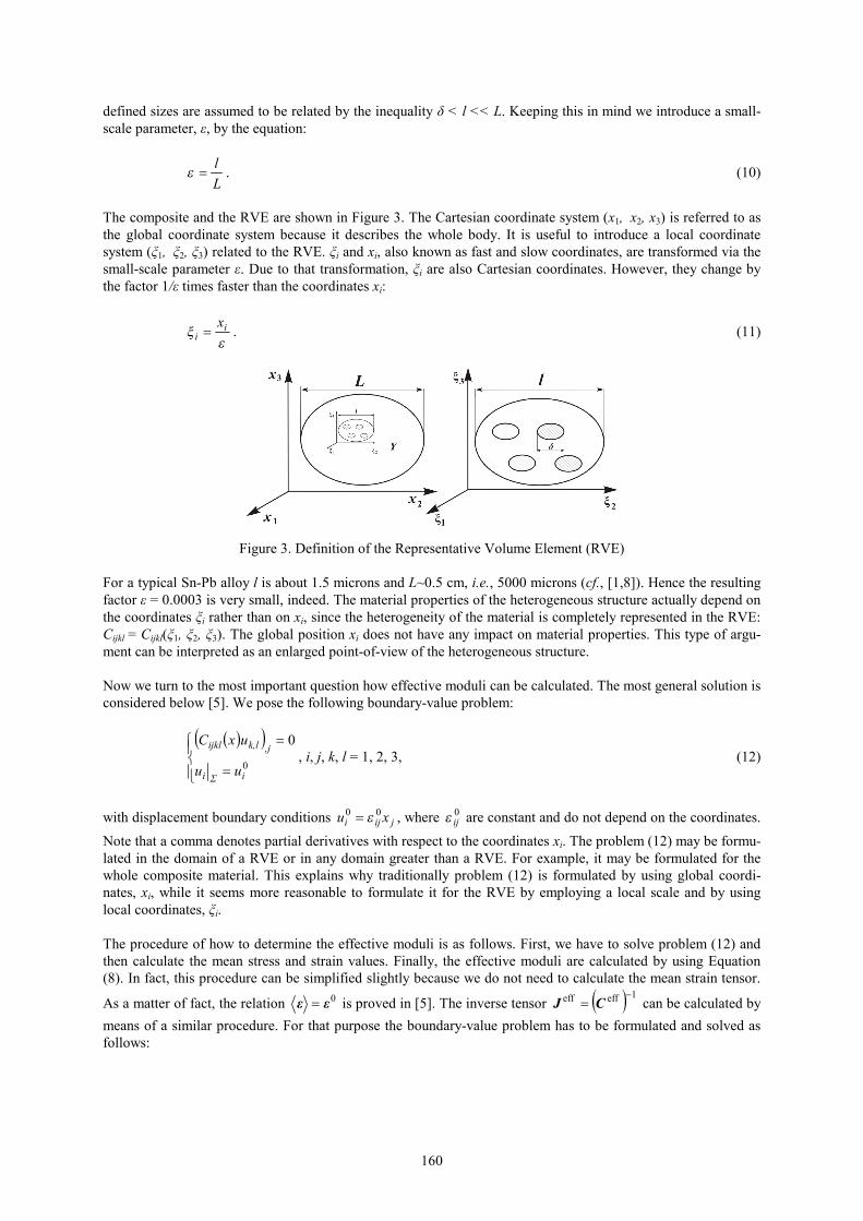
The composite and the RVE are shown in Figure 3. The Cartesian coordinate system (x1, x2, x3) is referred to as the global coordinate system because it describes the whole body. It is useful to introduce a local coordinate system (ξ1, ξ2, ξ3) related to the RVE. ξi and xi, also known as fast and slow coordinates, are transformed via the small-scale parameter ε. Due to that transformation, ξi are also Cartesian coordinates. However, they change by the factor 1/ε times faster than the coordinates xi:

ε

ξ ii

x= . (11)

Figure 3. Definition of the Representative Volume Element (RVE)

For a typical Sn-Pb alloy l is about 1.5 microns and L~0.5 cm, i.e., 5000 microns (cf., [1,8]). Hence the resulting factor ε = 0.0003 is very small, indeed. The material properties of the heterogeneous structure actually depend on the coordinates ξi rather than on xi, since the heterogeneity of the material is completely represented in the RVE: Cijkl = Cijkl(ξ1, ξ2, ξ3). The global position xi does not have any impact on material properties. This type of argu-ment can be interpreted as an enlarged point-of-view of the heterogeneous structure. Now we turn to the most important question how effective moduli can be calculated. The most general solution is considered below [5]. We pose the following boundary-value problem:

( )( )

=

=

0

0

iΣi

,jk,lijkl

uu

uxC, i, j, k, l = 1, 2, 3, (12)

with displacement boundary conditions jiji xu 00 ε= , where 0

ijε are constant and do not depend on the coordinates. Note that a comma denotes partial derivatives with respect to the coordinates xi. The problem (12) may be formu-lated in the domain of a RVE or in any domain greater than a RVE. For example, it may be formulated for the whole composite material. This explains why traditionally problem (12) is formulated by using global coordi-nates, xi, while it seems more reasonable to formulate it for the RVE by employing a local scale and by using local coordinates, ξi. The procedure of how to determine the effective moduli is as follows. First, we have to solve problem (12) and then calculate the mean stress and strain values. Finally, the effective moduli are calculated by using Equation (8). In fact, this procedure can be simplified slightly because we do not need to calculate the mean strain tensor.

As a matter of fact, the relation 0εε = is proved in [5]. The inverse tensor ( ) 1effeff −= CJ can be calculated by

means of a similar procedure. For that purpose the boundary-value problem has to be formulated and solved as follows:

161

( )( )

=

=

,SnuC

uxC

iΣjk,lijkl

,jk,lijkl 0 (13)

where jiji nS 0σ= and 0

ijσ denotes constant stresses. Next the mean strains ijε have to be calculated and, fi-

nally, effective compliances effJ are determined by using the following equation: klijklij J σε eff= . (14)

It is relatively easy to prove that 0σσ = (see [5] for details). It seems reasonable to defines the tensor effC of

Equation (8) as the inverse to effJ defined by the previous equation. Of course, these procedures are usually implemented only approximately. However, this allows deriving closed-form solutions for the effective moduli. For example, several effective moduli calculation methods employ the ESHELBY solution [5] and allow deriving formulae for composites reinforced by inclusions or by fibers. Note that such formulae provide high accuracy only for small volume fractions of inclusions. Another approach is based on a numerical solution to the boundary-value problem (12). Certainly, a numerical solution is approximate by its very nature. However, its accuracy does almost not depend on the volume fractions of the inclusions or fibers. Laminates seem to be the only example of a composite medium for which exact closed-form formulae have been derived. They are described in the next section within the framework of the so-called multi-scale method. 4 Multi-Scale Method Some composite materials show a periodic structure. Such a material is composed of a repetitive element which is called periodicity cell. As a matter of fact a periodic cell is the RVE itself. Periodic structures lead to signifi-cant simplifications of the solution of problem (12) because it has to be solved only in a domain of one periodic-ity cell [9]. This is described below with the help of a multi-scale method which utilizes the idea of two scales [6,7]. Indeed, composite materials with periodic structures can be investigated by using at least two scales. The global scale is related to the whole piece of the material. Hence global coordinates, xi, are used to identify mate-rial points. The local scale is related to the periodicity cell only. Consequently, ‘fast’ coordinates, ξi, are em-ployed at this level in order to account for the microstructure. A two-scale method effectively utilizes two differ-ent scales and represents a solution depending on both ‘slow’ and ‘fast’ coordinates to the global boundary value problem by combination of functions, e.g., a slow-varying global displacement field superposed with a fast-varying local displacement field. Indeed, elastic moduli depend on the periodicity of the cell structure, i.e., on ‘fast’ coordinates only so that Cijkl = Cijkl(ξ1, ξ2, ξ3). Often moduli ( )ξijklC are treated as discontinuous piece-vise

constant functions of the coordinates ξ . On the other hand, the right-hand side in the equilibrium equation de-pends usually on ‘slow’ coordinates. Therefore the solution to a boundary-value problem depends on both coor-dinates as indicated by the following formula: ( )( ) ( )( ) ( )( ) ...,uε,uε,uu iiii +++= ξxξxξx 2210 (15) The multi-scale method is based on the idea of representing the solution of the elasticity problem as an asymp-totic series [7]. Equation (15) states that the displacement is represented by an asymptotic series with respect to small parameter ε: the higher the number of periodicity cells, the smaller the parameter ε. After some modifications, see [6] for Details, the series is simplified to the form: ( ) ( ) ( ) ( ) ...νNεν,u j,kijkii ++= xξxξx (16) where ( )xν is the slow-varying displacement part while ( )ξijkN represents the fast-varying displacement fluc-tuations. According to the asymptotic nature of the series the first two terms are already sufficient to get a good accuracy for the displacement with a small ε.

162

Multi-scale methods were developed for solutions of differential equations with fast-varying coefficients, such as the equilibrium equation of linear elasticity: ( )( ) ( ) 0

,, =+ xξ ijlkijkl fuC . (17)

In particular multi-scale method is used to determine the effective elastic moduli for a periodic medium. With this purpose in mind we substitute the displacement (15) in (13) and collect terms for every power of small pa-rameter ε. The major term has the factor ε-1 and must be equal to zero because mathematically speaking ε tends to zero. These results lead to the following relation, which is usually referred to as the cell problem [6,7]:

( ) ( ) ( ) 0=

+

∂

∂

∂∂ ξ

ξξ ijpq

i

ipqijkl

iC

NC

ξξ, p, q = 1, 2, 3. (18)

This allows us to determine the local displacement functions ( )ξipqN . These functions represent displacements inside the periodic cell. Hence the first subscript denotes the direction of the displacement. The last two sub-scripts are free and remind us that six local problems have to be solved in the most general case. The equilibrium relation (17) is supplemented by boundary conditions and a condition ( ) 0=ξipqN . The latter

equality simply means that ( )xν is equal to the mean value of displacement ( )ξx,iu according to Equation (16). Very often the periodicity cell is a square so that the boundary conditions are periodicity conditions in the sense that the functions ipqN and their derivatives are the same on the left and right hand side faces of the periodicity cell. Certainly the same is true about the top and the bottom, front, and back faces, respectively. The second outcome from the substitution of (15) into the equilibrium equation is the homogenized equilibrium equation with effective moduli eff

ijpqC as coefficients: ( ) ( ) 0

,,eff =+ xijlkijkl fuC . (19)

This equation is the result of averaging over the periodicity cell of all terms that are multiplied by ε0 in the equi-librium equation after substituting the displacements following (15). Strains and stresses are determined by means of the following formulae:

( ) qpi

jpq

j

ipqijjiij v

NNvv ,,, 2

121

∂

∂+

∂

∂++=

ξξε , ( ) ( ) ( )ξ

ξξ ijpq

l

kpqijklij C

NC +

∂

∂=

ξσ (20)

which are derived by direct differentiation of the displacements (15). Now it is easy to understand why the multi-scale method presents a way to calculate effective moduli as addi-tional outcome. In fact, if it is used to solve the boundary-value problem (12), some simplifications will arise. In such a case, the linear displacements jiji xv 0ε= give an exact solution to the homogenized equilibrium equation and satisfy the boundary conditions in the boundary-value problem (12). Therefore, stresses and strains in prob-lem (12) are given by (20).

Then, their mean values are as given by ( ) ( ) ( ) 0pqijpq

i

kpqijklij C

NC ε

ξσ ξ

ξξ +

∂

∂= , 0

pqij εε = and, effective

elasticity moduli have the following form:

( ) ( ) ( )ξξξ ijpq

l

kpqijklijpq C

NCC +

∂

∂=

ξeff . (21)

163

Now we consider a laminated composite material as shown schematically in Figure 4a. We choose x3(ξ3) to be situated across the direction of the layers. The periodicity cell is composed of several layers of different materi-als. In this case the local equation (18) appears to be an ordinary differential equation. Its solution followed by averaging results in an exact closed-form formula for effective moduli:

nkiimijmnkqqppiimijmijnkijnk CCCCCCCCCC 31

33331

3311

331

333eff −−−−− −+= . (22)

Figure 4. a) Model layered structure; b) Tin-lead solder structure

In Figure 4b we can see a Sn-Pb solder structure composed of tin and lead layers. In the next section we use two approaches for calculating its effective moduli. First, we use the finite element method to solve (12) in the RVE directly. Second, we use Equation (22) because the solder structure is very similar to a layered structure as can be seen in Figure 4b. In the case of plane elasticity the formulae simplify to become:

.

,

,

,

112323

eff2323

133332233

113333

eff2233

113333

eff3333

13333

22233

2133332233

1133332222

eff2222

−−

−−−

−−

−−−−

=

=

=

−+=

CC

CCCC

CC

CCCCCCC

(23)

By taking into account that the solder under consideration is composed of two phases with volume fractions 1v and 2v , respectively, we get:

[ ] [ ] ,)2(3333

22)2(2233)1(

3333

12)1(2233)1(

33332)2(

33331

)2(3333

)1(3333

2

)2(3333

2)2(2233)1(

3333

1)1(2233

)2(22222

)1(22221

eff2222

CvC

CvC

CvCvCC

CvC

CvC

CvCvC

⋅−⋅−⋅+⋅

⋅

+

+⋅+⋅=

.

,

,

)1(33332

)2(33331

)2(3333

)1(3333

)2(3333

)2(2233

2)1(3333

)1(2233

1eff2233

)1(23232

)2(23231

)2(2323

)1(2323eff

2323

)1(33332

)2(33331

)2(3333

)1(3333eff

3333

CvCvCC

CC

vCC

vC

CvCvCC

C

CvCvCC

C

⋅+⋅

⋅⋅

⋅+⋅=

⋅+⋅

⋅=

⋅+⋅

⋅=

(24)

164

5 Effective Elastic Properties of a SnPb-Alloy Traditionally tin-lead alloys are widely used as microelectronic solders. Micro-structural diffusion occurs during the lifetime of the solder due to various external influences. Consequently, the structure of the alloy changes and this, in turn, leads to changing material properties. In this section we conduct a relatively simple study in order to answer the question of how much the solders effective moduli of elasticity change depending on a micro-structural variation. A more advanced study on homogenization of the change of the plastic properties of alloys will be presented in a later paper. Then it will be investigated how significantly homogenized yield stresses and tangent moduli depend on micro-structural change. Certainly, the most challenging question concerns the forma-tion of cracks, voids or other type of damage that can result in the solder destruction and the breakdown of the functionality of the component. For the purpose of finding the effective elastic moduli we consider a tin-lead alloy as a two-phase (or two-component) composite structure as shown in Figure 5. The sequence of pictures in this figure shows the devel-opment of the microstructure over time. These micrographs have been generated by solving an extended diffu-sion equation to predict the local concentrations of the constituents of the solder [8]. In addition to the classical driving force for phase separation introduced by CAHN-HILLIARD, an additional term has been introduced, which accounts for the coupling of the mechanical and the thermodynamical problem. The pictures show the typical lamella-type structure of SnPb solders, which occur due to the tetragonal crystal symmetry of the Sn-specimen. Sampling moments of the pictures in Figure 5 are 0.2, 0.5, 1.0, 2.0, 5.0, 10.0 and 20.0 seconds, respectively. The solder is quenched from 183°C down to the 20°C without mechanical loads: No external stresses, which would have an impact on coarsening rate and the developing microstructure, have been applied. One can see that the phases become larger during diffusion. However, due to mass conservation, the volume ratios of the phases are close to constant with quite good accuracy as shown in Table 3. More information about the coarsening in SnPb solders can be found in [8].

Effective elastic moduli of SnPb ( )GPa Volume fraction Time (s) 2222C 2233C 3333C 2323C Sn Pb

0.1 68.118 43.13975 57.89635 17.33439 0.418747 0.581253 0.2 68.28854 43.14284 57.97969 17.35716 0.421997 0.578003 0.5 68.42638 43.15011 58.04856 17.3767 0.425079 0.574921 1 68.65148 43.15441 58.15837 17.40665 0.430038 0.569962 2 68.53788 43.15237 58.10065 17.39099 0.427139 0.572861 5 68.79415 43.16218 58.23107 17.42867 0.431854 0.568146 10 68.91313 43.08686 58.20988 17.41485 0.430069 0.569931 20 69.1416 43.01026 58.24527 17.41563 0.430725 0.569275

Table 3. Effective moduli of SnPb at different times

Figure 5. Tin-lead alloy structure change caused by diffusion We conducted calculations in order to study how much the effective elastic moduli change during the diffusion process. The two methods that we used in order to determine effective moduli of elasticity were explained in the previous section. First, we used a method based on direct numerical solution of the plane elasticity boundary-value problem (12) and formula (8). This formula now reads: ( )0eff

klijklij C εσ = , (25)

165

where ijσ are the average stresses of the RVE. It should be emphasized that this approach is just the numerical

implementation of the definition of effective moduli as given by Equations (12) and (8). If we put ( ) ( )αβαβ δεε 00 = ,

then we get effective moduli ( )αβαβ δεσ 0eff

ijijC = for 3,2,,, =βαji from (8). αβδ stands for Kronecker’s

delta. All subscripts assume the values 2, 3 because plane strain is assumed and the first axis is directed in per-pendicular direction. Second, we determined the effective moduli by using closed-form formulae (24) and kept in mind that the struc-ture of the alloy is similar to a layered composite. Note that the first method is general whereas the second one is only valid for structures similar to a layered setup. It is important to underline that both methods resulted in almost the same effective moduli values. The main re-sult of the calculations conducted can be formulated as follows: Microstructural change barely affects the out-come of the effective moduli. For example, Figure 6 gives the time dependence of modulus ( )tC2323 . Every value ( )tC2323 on the graph corre-sponds to the moment of time, for which the picture of the microstructure was provided. These pictures were obtained by means of diffusion simulation developed in [8]. The blue diamonds in Fig. 6 represent ( )tC2323 cal-culated when using the first method, while brown square points show the variation of 2323C in time determined from the closed-form formulae. The points are very close to each other so that the relative difference varies from 0.5% to 2%. Obviously, the closed-form formulae developed for layered material provide a good approximation tool for the effective moduli of the alloy. We also observe that all effective moduli vary very little. As an exam-ple the effective modulus 2323C will be examined in more depth. Its changes are comparable to the changes in phase volume ratios or to the accuracy of calculations. Table 3 shows the effective moduli calculated at different times of the structure of the alloy shown in Fig. 5. Two conclusions can be drawn. First, the effective moduli of the alloy depend only on volume fractions of the phases but not on the detailed structure of the alloy. Second, the effective moduli do not change during diffusion.

Figure 6. Variation of the effective modulus 2323C during diffusion

Fig. 7 shows the relative difference numericalC

C∆ in moduli calculated using the two different methods explained

above. The difference appears to be smaller towards the end of the diffusion process. However, this result is questionable since the difference is very small and comparable to the accuracy of the calculations and within the “discretization noise” of the picture.

166

Figure 7. Relative difference between effective moduli

6. Effective Moduli of a Composite with Inclusions We studied the dependence of the effective moduli on a composite structure containing a varying volume fraction of tin Tinc in the range 0.14 to 0.41 by using the two approaches again. The first method is based on closed-form formulas for fibrous composite taken from [5], while the second one employs direct numerical simulation, i.e., it is numerical solution of the boundary-value problem (12) in the same way as described in previous section. In order to do this a computer program was written, which generates different composite structures. All inclu-sions are assumed to be circles of different radii. The generated RVEs are shown in Figures 8 - 10.

Figure 8. The set of regular structures where inclusions are aligned with nodes of square grid

Figure 9. The set of regular structures where inclusions are aligned with nodes of triangular grid

167

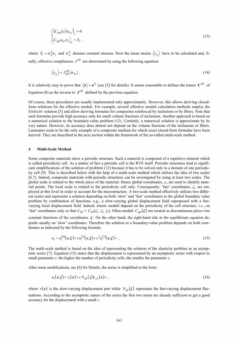
Figure 10. The set of irregular structure Tin inclusions are shown in the figures as white circles. We considered three types of structures: Two of them are periodical and the third one is irregular. In the case of periodical structures, the centers of the inclusions are aligned along a regular grid. We use grids with square and triangular patterns. In the case of an irregular grid, the grid nodes are distributed according to random deviations from the square grid nodes. The computer program developed allows generating composite structure of these types for given volume fraction of tin and RVE size. The volume fractions of composite structures shown in Figures 8 – 10 are given in Table 5.

a) 14.0Tin =c b) 28.0Tin =c c) 41.0Tin =c d) 14.0Tin =c e) 28.0Tin =c f) 41.0Tin =c

Table 5. Volume fractions of the composite structures in Fig. 8-10

It seems reasonable to give a few more details regarding the first method. The formulae for effective moduli for structures that are shown in Figures 8 - 10 can be easily obtained by using the well-developed theory of unidirec-tional fiber composites. Indeed, we can assume that the fibrous composite is such that the fibers are directed perpendicular to the planes shown in Figures 8 - 10. With this idea in hand, we apply formulae for the in-plane effective moduli from [5], as an example. The plane that is perpendicular to the fibers is isotropic for a homoge-nized material in the case of structures with triangular and random inclusions distribution. On the other hand, it is orthotropic for square grid structures. All formulae that we are going to employ were developed for fibrous com-posites that are transversally-isotropic in macro-scale. This means they can be employed for structures shown in Figures 9 - 10. In the case of a square grid (see Fig. 8) they only provide a way of getting an approximation for the effective moduli and the accuracy that they provide has to be discussed. On the other hand, in contrast to the formulae for the layered medium, which were taken from fibrous composite theory, they are approximate even for triangular and random grid nodes distribution. The accuracy decreases with the growth of volume fraction. Therefore, it seems that the same formulae can be used approximately in the case of square nodes distribution. In fibrous material theory fibers are usually assumed to be randomly distributed in cross-plane, so it is isotropic in terms of effective homogeneity. Therefore, there are two independent elasticity moduli: the bulk modulus 23K and the shear modulus 23µ in that plane. Consequently, the relationship of different moduli in the plane of isot-ropy is as follows [5]:

.

,

,

eff23

eff2323

eff23

eff23

eff2233

eff23

eff23

eff3333

eff2222

µ

µ

µ

=

+−=

+==

C

KC

KCC

(26)

Hence the task is to get the closed-form formulae for in-plane bulk and shear moduli. The formula for the effec-tive bulk modulus, eff

23K , was derived in [10, 11] and the one for the effective shear modulus , eff23µ , was derived

in [12]:

168

( )

1

Lead34

Lead

Tin

LeadTin31

LeadTinTin

LeadLead

eff23

113

−

+−

+−+−

⋅++=µµµ

µk

ckk

ckK , (27)

++

+−

⋅+⋅=−1

Lead38

Lead

Lead37

Lead

LeadTin

LeadTinLead

eff23 2

1µ

µµµ

µµµ

kk

c . (28)

It should be pointed out that the formula for eff

23µ is correct only for a volume fraction of inclusion that is not greater than 0.2. For greater volume fractions the calculations are slightly more complicated and quadratic equa-tions have to be solved [5]. The approximate nature of the formulae we use is a reason for comparing both approaches and evaluating the accuracy of the closed-form formulas. Effective moduli calculated by using direct numerical calculation are given in Table 6. VF N 2222C 2233C 3333C 2323C Mesh Sq Tr R Sq Tr R Sq Tr R Sq Tr R

49 109.19 108.83 107.37 57.39 58.03 58.15 109.19 109.2 107.36 25.09 25.36 24.89 25 110.73 109.19 107.73 57.74 58.15 58.03 110.73 108.98 108.73 25.9 25.25 24.67 16 110.82 108.97 107.6 57.65 57.87 57.93 110.82 108.67 107.47 26.35 25.41 24.78 9 112.4 109.58 108.76 57.96 57.92 58.06 112.4 109.3 107.6 27.54 25.83 25.49

0.14

4 116.25 111 107.37 58.83 58.04 57.73 116.25 110.75 108.01 30.29 26.87 24.73

144 137.86 135.62 135.16 66.55 68.98 68.65 137.86 134.66 138.02 30.19 31.18 31.17 36 137.56 134.98 134.22 66.76 68.72 67.75 137.56 134.25 134.65 31.54 31.59 30.66 16 139.17 138.8 134.91 67.16 68.71 68.42 139.17 135 133.7 33.47 32.49 32.23 9 141.78 137.09 137.25 67.85 68.22 67.91 141.78 136.48 133.54 35.86 34.43 32.08

0.28

4 148.27 138.84 135.16 69.7 68.06 68.52 148.27 136.23 135.2 41.25 34.96 33.55

144 167.83 164.94 164.77 75.48 79.76 78.11 167.83 161.75 169.56 35.5 37.97 36.99 36 169.34 169.97 167.09 76.52 80.07 79.96 169.34 162.03 167.85 37.55 39.31 39.33 16 171.88 173.29 166.57 77.49 80.45 80.15 171.88 163.79 169.3 40.29 40.84 40.28 9 174.86 176.67 171.89 78.52 80.75 79.42 174.86 165.79 170.97 43.42 42.5 41.39

0.41

4 182.84 183.9 164.89 81.21 81.65 78.52 182.84 169.98 170.54 50.67 46.08 39.76

64 204.72 202.82 203.68 86.46 92.58 90.41 204.72 198.28 208.41 42.32 47.11 44.73 0.5 25 205.19 205.98 200.95 87.47 93.08 90.75 205.19 201.69 206.59 44.84 48.94 45.66

Table 6. Effective moduli for different distributions of inclusions

In Table 6 VF stands for the Volume Fraction of Sn (tin), Sq means SQuare grid, Tr and R refer to TRiangular and Random grids, respectively; N is the number of inclusions. An analysis of the results given in the Table 6 leads to the following conclusions: The first one concerns the RVE size. It could be revealed that the RVE must include at least four inclusions for a regular square grid. For a regu-lar triangular grid and an irregular grid the RVE can be smaller. This is true for any considered volume. Once the ratio is constant the effective moduli change little if the RVE size increases. The relative difference is about 1%. Therefore, we can conclude that the effective moduli within the RVE depend on the volume fractions of the phases only. Moreover, if the volume fraction is constant, the effective moduli do not depend on the grid type, too. As an example the modulus ( )cC2222 is shown in Figure 11 as a function of the volume fraction, c, of the inclu-sions. Again the modulus was determined by using the numerical method based on a solution of the boundary-value problem (11) and by approximate closed-form expressions valid for small fibers volume fractions. The

169

numerically determined modulus ( )cC2222 is indicated by a dotted line. The modulus calculated by virtue of closed-form expressions is represented by a solid line.

Figure 11. Tin volume fraction dependence of 2222C

The graphs for the other effective moduli are qualitatively the same. It is clear that the closed-form solutions provide a good approximation only for volume fractions of the inclusions that are less than 0.2. Within this range the accuracy of the formulae is less than 5%. It should be noted that the accuracy of the formulae (23) for the structure shown in Figure 5 is about 0.5%-2%. The second remark concerns the effect of different distributions of inclusions. Figure 9 shows that the effective moduli calculated for square, triangle and random grids are very close to each other. This simply means that the effective moduli depend on the volume ratio of the inclusions and that they do not depend on the details of the distribution of the inclusions. The number of the inclusions and their alignment shows no impact on effective moduli. The calculations described in this section validate once again that the structural change during the diffusion proc-ess does not influence the effective moduli of elasticity of a solder. 7 Conclusion and Outlook As it was shown in Section 2 of this paper, the geometry and therefore the distribution of the constituents in the microstructure has an influence on mechanical properties which cannot be neglected. Moreover the analysis of the results of the multi-scale approach clearly shows that a microstructure changing with time has no influence on the elastic properties. This can be interpreted in the following manner. Since in the presented solder alloys the type of the microstructure (e.g., lamellae, grains of essentially circular shape) does not change during the coars-ening process and just the geometric distribution of the structures is different, the elastic parameters are constant over time. Nevertheless, although the development in time can be neglected, the influence of the microstructure on elastic properties is of interest due to formation of certain geometries in the early stages of phase separation. An alloy that develops a lamella-type of microstructure will give different effective elastic moduli than, e.g., an alloy composed of cubic constituents that will form a grain-type microstructure although the concentrations of inclusions might be the same. Note that the presented results just hold for elastic properties. Non-linear material laws for plastic and creep deformations are a topic of current interest. As the presented multi-scale method has been proven to be a powerful tool for that kind of structures, an adaption for non-linear material behavior is re-quired. As solders are frequently subjected to the thermo-mechanical fatigue loading, further examinations are aimed to apply the presented methods to such kind of material behavior.

170

References [1] Müller, W.H., Böhme, T:. Quantitative description of micro-structural changes in lead-free solder alloys.

Electronics Packing Technology Conference, 390–397, 2006. [2] Böhme, T., Dreyer, W., Müller, W.H.: Determination of higher gradient coefficients by means of the Embed-

ded-Atom-Method, Cont. Mech. Thermodyn., 18, 411-441, 2007. [3] Nye, J.F.: Physical properties of cystals, Oxford University Press, 140-145, 1957. [4] Hashin, Z., Shtrikman, S.: A variational approach to the theory of the elastic behaviour of multiphase materi-

als, J. Mech. Phys. Solids, 11, 127-140, 1963. [5] Christensen, R.M.: Mechanics of composite materials. J. Wiley, 2nd ed., 1979. [6] Pobedrya, B.E.: Mechanics of composite materials. Moscow State University Press, 1984 (in Russian). [7] Bakhvalov, N.S., Panacenko, G.P.: Homogenization: Averaging processes in periodic media. Mathematical

problems in the mechanics of composite materials, Kluwer Academic Publishers, Dordrecht, 1994. [8] Dreyer, W., Müller, W.H.: A study of the coarsening in tin/lead solders. International Journal of Solids and

Structures, 37, 3841-3871, 2000. [9] Bardzokas, D.I.: Mathematical modelling of physical processes in composite materials of periodical struc-

tures. URSS Editorial, 2003. [10] Hill, R.: Theory of mechanical properties of fibre-reinforced materials. I. Elastic behaviour. J. Mech. and

Phys. Solids, 1964, v.2, p. 166. [11] Hashin Z. Viscoelastic fiber reinforced materials. AIAA Journal, 1966, V.4, p.1411. [12] Christensen R.M., Lo K.H. Solutions for effective shear properties in three phase sphere and cylindrical

models. J. Mech. and Phys. Solids, 1979, v.27, No.4 _________________________________________________________________________________________ Addresses: Dipl.-Ing. Andreas Brandmair, Technische Universität Berlin, Fak. V, Institut für Mechanik, Lehrstuhl für Kontinuumsmechanik und Materialtheorie, MS2, Einsteinufer 5, D-10587 Berlin, email: andreas.brandmair@tu-berlin.de Prof. Wolfgang H. Müller, Technische Universität Berlin, Fak. V, Institut für Mechanik, Lehrstuhl für Konti-nuumsmechanik und Materialtheorie, MS2, Einsteinufer 5, D-10587 Berlin, email: wolfgang.h.mueller@tu-berlin.de Margerita Savenkova, Lomonosov Moscow State University, GSP-2, Leninskie Gory, Moscow, 119992, Russia, email: madgista@gmail.com Prof. Sergey Sheshenin, Lomonosov Moscow State University, GSP-2, Leninskie Gory, Moscow, 119992, Russia, email: sergey.sheshenin@mail.ru