A Measurement of the Gluon Distribution in the Proton and of
143
A Measurement of the Gluon Distribution in the Proton and of the Strong Coupling Constant α s from Inclusive Deep-Inelastic Scattering Dissertation zur Erlangung der naturwissenschaftlichen Doktorw¨ urde (Dr. sc. nat.) vorgelegt der Mathematisch-naturwissenschaftlichen Fakult¨ at der Universit¨ at Z ¨ urich von Rainer Wallny aus Deutschland Begutachtet von Prof. Dr. Ulrich Straumann Dr. habil. Max Klein Z¨ urich 2001
Transcript of A Measurement of the Gluon Distribution in the Proton and of
A Measurementof the Gluon Distribution in the Proton
and ofthe Strong Coupling Constant αs
from Inclusive Deep-Inelastic Scattering
Dissertationzur
Erlangung der naturwissenschaftlichen Doktorwurde(Dr. sc. nat.)
vorgelegt derMathematisch-naturwissenschaftlichen Fakultat
der
Universitat Zurich
von
Rainer Wallnyaus
Deutschland
Begutachtet vonProf. Dr. Ulrich Straumann
Dr. habil. Max Klein
Zurich 2001

Die vorliegende Arbeit wurde von der Mathematisch-naturwissenschaftlichen Fakultat der Uni-versitat Zurich auf Antrag von Prof. Dr. Ulrich Straumann und Prof. Dr. Peter Truol alsDissertation angenommen.

To the memory of my father

Abstract
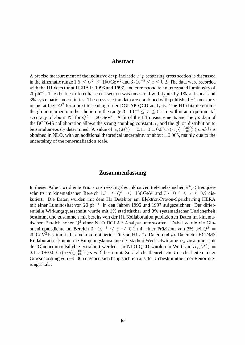
A precise measurement of the inclusive deep-inelastic e+p scattering cross section is discussedin the kinematic range 1.5 ≤ Q2 ≤ 150 GeV2 and 3 ·10−5 ≤ x ≤ 0.2. The data were recordedwith the H1 detector at HERA in 1996 and 1997, and correspond to an integrated luminosity of20 pb−1. The double differential cross section was measured with typically 1% statistical and3% systematic uncertainties. The cross section data are combined with published H1 measure-ments at high Q2 for a next-to-leading order DGLAP QCD analysis. The H1 data determinethe gluon momentum distribution in the range 3 · 10−4 ≤ x ≤ 0.1 to within an experimentalaccuracy of about 3% for Q2 = 20 GeV2 . A fit of the H1 measurements and the μp data ofthe BCDMS collaboration allows the strong coupling constant αs and the gluon distribution tobe simultaneously determined. A value of αs(M
2Z) = 0.1150 ± 0.0017(exp)+0.0009
−0.0005 (model) isobtained in NLO, with an additional theoretical uncertainty of about ±0.005, mainly due to theuncertainty of the renormalisation scale.
Zusammenfassung
In dieser Arbeit wird eine Prazisionsmessung des inklusiven tief-inelastischen e+p Streuquer-schnitts im kinematischen Bereich 1.5 ≤ Q2 ≤ 150 GeV2 and 3 · 10−5 ≤ x ≤ 0.2 dis-kutiert. Die Daten wurden mit dem H1 Detektor am Elektron-Proton-Speicherring HERAmit einer Luminositat von 20 pb−1 in den Jahren 1996 und 1997 aufgezeichnet. Der differ-entielle Wirkungsquerschnitt wurde mit 1% statistischer und 3% systematischer Unsicherheitbestimmt und zusammen mit bereits von der H1 Kollaboration publizierten Daten im kinema-tischen Bereich hoher Q2 einer NLO DGLAP Analyse unterworfen. Dabei wurde die Glu-onenimpulsdichte im Bereich 3 · 10−4 ≤ x ≤ 0.1 mit einer Prazision von 3% bei Q2 =20 GeV2 bestimmt. In einem kombinierten Fit von H1 e+p Daten und μp Daten der BCDMSKollaboration konnte die Kopplungskonstante der starken Wechselwirkung αs zusammen mitder Gluonenimpulsdichte extrahiert werden. In NLO QCD wurde ein Wert von αs(M
2Z) =
0.1150± 0.0017(exp)+0.0009−0.0005 (model) bestimmt. Zusatzliche theoretische Unsicherheiten in der
Grossenordung von ±0.005 ergeben sich hauptsachlich aus der Unbestimmtheit der Renormie-rungsskala.
iv
Contents
1 Perturbative QCD and Deep Inelastic Scattering 4
1.1 Deep Inelastic Scattering . . . . . . . . . . . . . . . . . . . . . . . . . . . . . 4
1.2 Bjorken Scaling . . . . . . . . . . . . . . . . . . . . . . . . . . . . . . . . . . 5
1.3 Quark Parton Model . . . . . . . . . . . . . . . . . . . . . . . . . . . . . . . 6
1.4 Quantum Chromodynamics . . . . . . . . . . . . . . . . . . . . . . . . . . . . 8
1.4.1 The Running Coupling Constant . . . . . . . . . . . . . . . . . . . . . 8
1.4.2 Factorisation . . . . . . . . . . . . . . . . . . . . . . . . . . . . . . . 12
1.4.3 F2 and FL in next-to-leading order QCD . . . . . . . . . . . . . . . . . 13
1.5 DGLAP Evolution and (∂F2/∂ ln Q2)x . . . . . . . . . . . . . . . . . . . . . 14
2 An Accurate Cross Section Measurement at Low x 19
2.1 Extraction of the Cross Section . . . . . . . . . . . . . . . . . . . . . . . . . . 19
2.2 Kinematic Reconstruction . . . . . . . . . . . . . . . . . . . . . . . . . . . . 20
2.3 Data Analysis with the H1 Detector . . . . . . . . . . . . . . . . . . . . . . . 22
2.3.1 Datasets . . . . . . . . . . . . . . . . . . . . . . . . . . . . . . . . . . 22
2.3.2 Event Selection Strategy . . . . . . . . . . . . . . . . . . . . . . . . . 24
2.3.3 Electromagnetic Energy Calibration . . . . . . . . . . . . . . . . . . . 26
2.3.4 Photoproduction Background . . . . . . . . . . . . . . . . . . . . . . 26
2.3.5 Hadronic Energy Scale . . . . . . . . . . . . . . . . . . . . . . . . . . 26
2.4 Systematic Errors . . . . . . . . . . . . . . . . . . . . . . . . . . . . . . . . . 28
i
3 QCD Analysis Procedure 31
3.1 Analysis Procedure . . . . . . . . . . . . . . . . . . . . . . . . . . . . . . . . 31
3.1.1 Singlet and Non-Singlet Evolution of F2 . . . . . . . . . . . . . . . . 31
3.2 Flavour Decomposition . . . . . . . . . . . . . . . . . . . . . . . . . . . . . . 34
3.2.1 Simplified Ansatz . . . . . . . . . . . . . . . . . . . . . . . . . . . . . 34
3.2.2 Generalisation . . . . . . . . . . . . . . . . . . . . . . . . . . . . . . 35
3.3 Parameterisation . . . . . . . . . . . . . . . . . . . . . . . . . . . . . . . . . 36
3.3.1 Ansatz . . . . . . . . . . . . . . . . . . . . . . . . . . . . . . . . . . 36
3.3.2 Choice of Parameterisations . . . . . . . . . . . . . . . . . . . . . . . 38
3.3.3 Input Scale Dependence and χ2 Saturation . . . . . . . . . . . . . . . . 42
3.3.4 Gluon Momentum Fraction . . . . . . . . . . . . . . . . . . . . . . . 50
3.4 Definition of Minimization Procedure . . . . . . . . . . . . . . . . . . . . . . 54
3.4.1 Definition of χ2 . . . . . . . . . . . . . . . . . . . . . . . . . . . . . 54
3.4.2 Correlated Systematic Error Treatment . . . . . . . . . . . . . . . . . 54
3.4.3 Error Propagation . . . . . . . . . . . . . . . . . . . . . . . . . . . . . 55
4 Extraction of the Gluon Distribution 57
4.1 Quality of the Fits . . . . . . . . . . . . . . . . . . . . . . . . . . . . . . . . . 57
4.1.1 Comparison with the Data . . . . . . . . . . . . . . . . . . . . . . . . 57
4.1.2 Pull Distributions . . . . . . . . . . . . . . . . . . . . . . . . . . . . . 62
4.1.3 QCD Model Parameters . . . . . . . . . . . . . . . . . . . . . . . . . 62
4.1.4 Dataset Normalisation . . . . . . . . . . . . . . . . . . . . . . . . . . 66
4.1.5 Correlated Systematic Errors . . . . . . . . . . . . . . . . . . . . . . . 66
4.2 Effect of the Q2min Cut . . . . . . . . . . . . . . . . . . . . . . . . . . . . . . 69
4.3 Results . . . . . . . . . . . . . . . . . . . . . . . . . . . . . . . . . . . . . . . 73
4.4 Comparison to Heavy Quark Production Results . . . . . . . . . . . . . . . . . 80
4.4.1 Results for F cc2 in the NLO DGLAP Fits . . . . . . . . . . . . . . . . . 80
4.4.2 Heavy Quark Treament and Scheme Dependence . . . . . . . . . . . . 85
4.5 QCD Prediction for FL(x, Q2) and its Uncertainties . . . . . . . . . . . . . . . 86
ii
5 Determination of αs(M2Z) 93
5.1 αs(M2Z) from a Fit to H1 and BCDMS Data . . . . . . . . . . . . . . . . . . . 93
5.2 Systematic Effects in the BCDMS data . . . . . . . . . . . . . . . . . . . . . . 96
5.3 Fit to BCDMS data alone . . . . . . . . . . . . . . . . . . . . . . . . . . . . . 98
5.4 Effect of the Systematic Error Treatment on αs(M2Z) . . . . . . . . . . . . . . 103
5.5 αs(M2Z) from a Fit to H1 and NMC data . . . . . . . . . . . . . . . . . . . . . 106
5.6 Model Uncertainties . . . . . . . . . . . . . . . . . . . . . . . . . . . . . . . . 108
5.7 Results . . . . . . . . . . . . . . . . . . . . . . . . . . . . . . . . . . . . . . . 108
5.8 Theoretical Scale Uncertainty . . . . . . . . . . . . . . . . . . . . . . . . . . . 113
5.9 Further Cross Checks . . . . . . . . . . . . . . . . . . . . . . . . . . . . . . . 113
5.10 αs(M2Z) and the Gluon Distribution at High x . . . . . . . . . . . . . . . . . . 119
Summary 128
iii
Introduction
High Energy Physics is concerned with basically two tasks: the identification of the elemen-tary constituents of matter and the subsequent study of their properties, and with studying themechanisms by which these constituents interact with each other.
Experiments to pursue these objectives are nowadays performed by using high energy particleaccelerators, which accelerate particle beams to high energies and collide them with particles instationary “fixed” targets, or with particles in another beam. Around the intersection zones largedetectors are installed. These detect particle interactions by means of the energy deposition andthe tracks left by secondary particles scattered into the detector. The architecture of these detec-tors takes into account the type of accelerator they belong to; correspondingly one distinguishesfixed target experiments from colliding beam experiments, the latter covering almost the fullsolid angle 4π around the interaction zone.
In these high energy physics experiments, particle scattering cross sections, σ, are measuredand compared to theoretical predictions. These predictions are calculated as products of matrixelements squared containing the dynamics of the process under study and the lorentz-invariantphase space determined from the kinematics, i.e. energy and momentum conservation. The ma-trix elements in the language of quantum field theory are depicted as Feynman diagrams wherethe fundamental constituent fermions exchange virtual bosons which mediate their interaction.The correct theories describing these interactions are constructed using gauge invariance againstsymmetry transformations and are therefore also called gauge theories.
Constituent fermions are grouped in three families of quarks and three families of leptons.Together with the gauge bosons mediating the interactions, they form the ingredients of theso called Standard Model of particle physics which since the 1970s is the accepted theoreticalframework of high energy particle interaction phenomena.
The three forces known to dominate subatomic interactions1 are mediated by the massless pho-ton for the electromagnetic force, the three intermediate massive vector bosons Z 0, W+ and W−
for the weak and eight massless gluons for the strong force. The electromagnetic interactionhas very successfully been described by Quantum Electrodynamics (QED). Its generalisation toinclude weak effects leads to the electroweak gauge field theory. The strong force is describedby Quantum Chromodynamics (QCD), essentially a carbon copy of QED with important differ-ences concerning the coupling of the gauge bosons. For each interaction, a coupling constant αenters the theory as a parameter which has to be determined by experiment.
1The fourth interaction, gravitation, is too feeble to play a role in subatomic physics and is not easily incorpo-rated into the formalism of quantum field theory.
1
2
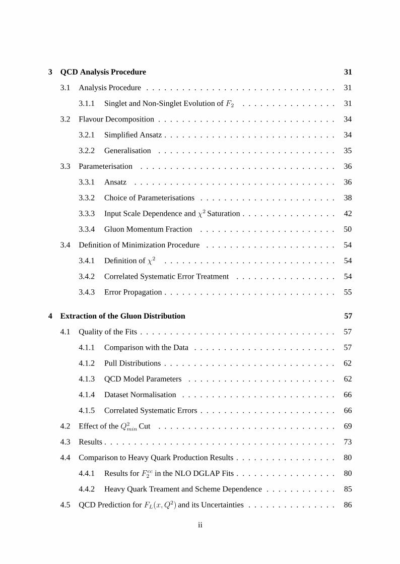
There are two scattering process types distinguished in high energy physics, spacelike and time-like scattering, see Figure 1. Timelike, or s-channel scattering is characterised by the center ofmass energy squared, s > 0. High center of mass energy can be converted to new and possiblyexotic particles found at higher mass scales. Timelike processes are the standard processes usedby particle factories. A typical timelike process is electron positron annihilation.
Spacelike scattering is characterised by the
e
e
Z0 / γ
e,μ,τ,q
e,μ,τ,q
A
e
e e
e
Z0 / γ
B
Figure 1: Feynman-Diagrams for production offermion pairs in e+e− collisions. A: timelike(s-channel). B: spacelike (t-channel).
four momentum squared t = q2 < 0 whichis transferred from one incident particle to theother. The exchanged virtual gauge bosonserves as a probe to survey the structure of theother particle. By virtue of the Heisenberguncertainty relation the negative four momen-tum squared Q2 = −q2 > 0, can be relatedto the resolution λ attained by such a probe,λ = 1/
√Q2. Thus spacelike processes
serve as microscopes. At HERA2, the electron proton collider at DESY, Hamburg, Germany,spatial dimensions of the order of 10−18 m can be resolved.
A classic spacelike process is deep inelastic scattering (DIS). In deep inelastic scattering, thestructure of nucleons can be studied by measuring the cross section of leptons scattering offnucleons, the building blocks of the atomic nucleus. Nucleons are found to consist of quarkswhich are bound together by gluons. It is the structure of the proton, the most abundant nucleon,and the interpretation of this structure in the framework of Quantum Chromodynamics, to whichthis thesis is devoted.
This work was performed with the H1 experiment installed in the North Hall of the HERAelectron-proton collider at DESY. In HERA, electrons or positrons with an energy of 27.5 GeVare brought to collisions with 820 GeV protons3 at a center of mass energy of about
√s ≈
300 GeV at the H1 interaction region and also at the South Hall housing another collider exper-iment, ZEUS. In Hall West and East, two fixed target experiments are installed, the HERA-Bexperiment dedicated to the study of CP-violation, and the HERMES experiment which is de-voted to the spin structure of the proton.
In this thesis, a measurement of the deep-inelastic electron proton scattering cross section atlow momentum transfers Q2 and low Bjorken x with the H1 detector at HERA is presentedand its interpretation performed in terms of Quantum Chromodynamics. After an introductionto the theoretical framework in chapter 1, the data analysis is briefly presented in chapter 2concentrating on the precision achieved due to the high luminosity of almost 20 pb−1 collectedduring data taking in 1996 and 1997.
The measured deep inelastic scattering cross section is then confronted with the prediction ofQuantum Chromodynamics. The analysis uses a new decomposition of the structure functionsinto parton distributions which avoids the use of deuteron data. This is described in chapter 3.
2Hadron Elektron Ring Anlage3the proton energy was raised to 920 GeV since the 1998 running period of HERA

3
The H1 data extend with high precision into a region where quarks and gluons carry very littlefractions of proton momentum, or Bjorken x. This is demonstrated to accurately determine thegluon momentum distribution. Results of this analysis are presented in chapter 4.
In a further step, accurate data at large Bjorken x from the muon proton scattering experimentBCDMS are combined with the H1 data and the strong coupling constant αs is extracted innext-to-leading order perturbation theory, chapter 5. Since the datasets are largely dominatedby systematic errors, a careful analysis of systematic uncertainties is performed.
The thesis is concluded with a short summary.
Chapter 1
Perturbative QCD and Deep InelasticScattering
1.1 Deep Inelastic Scattering
Deep inelastic electron proton scattering ep → eX is characterised by spacelike virtual gaugeboson exchange, with the virtuality of the exchanged gauge boson being larger than the protonmass squared, Q2 � M2
p . At four-momentum transfers Q2 � M2Z , the Born cross section is
dominated by one-photon exchange, since the competing weak interaction is suppressed by themass squared M2
Z of the intermediate vector boson Z0 entering the gauge boson propagator.
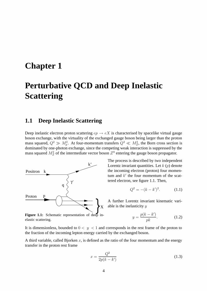
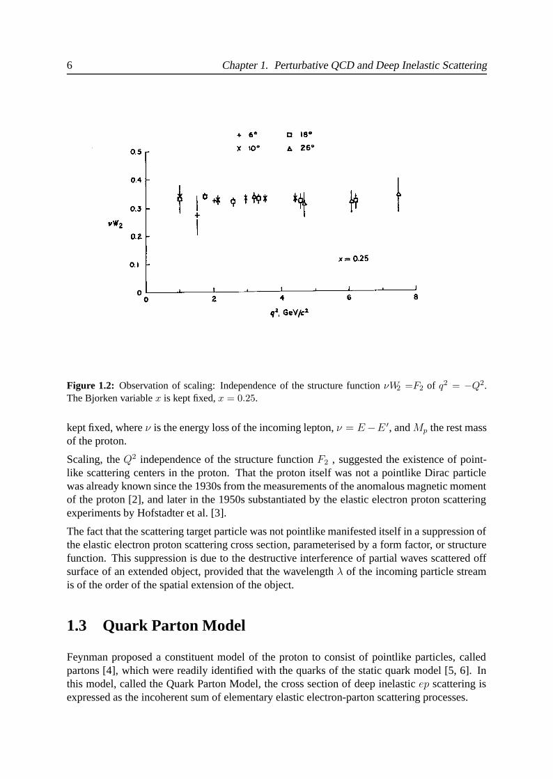
The process is described by two independent
}X
kPositron
Proton
k’
p
qγ∗
Figure 1.1: Schematic representation of deep in-elastic scattering.
Lorentz invariant quantities. Let k (p) denotethe incoming electron (proton) four momen-tum and k′ the four momentum of the scat-tered electron, see figure 1.1. Then,
Q2 = −(k − k′)2. (1.1)
A further Lorentz invariant kinematic vari-able is the inelasticity y
y =p(k − k′)
pk. (1.2)
It is dimensionless, bounded to 0 < y < 1 and corresponds in the rest frame of the proton tothe fraction of the incoming lepton energy carried by the exchanged boson.
A third variable, called Bjorken x, is defined as the ratio of the four momentum and the energytransfer in the proton rest frame
x =Q2
2p(k − k′)(1.3)
4
1.2. Bjorken Scaling 5
which is also dimensionless, bounded to 0 < x < 1 and related to y and Q2 and the center ofmass energy squared, s = (k + p)2 via the approximate relation
Q2 = xys (1.4)
neglecting the proton and the electron masses. In the Quark Parton Model, see below, thevariable x corresponds to the fraction of proton momentum carried by the parton which isstruck by the exchanged gauge boson.
The computation of the cross section ep → eX
σ ∼ LαβW αβ (1.5)
comprises the leptonic tensor Lαβ describing the lepton-gauge boson vertex which can be com-pletely calculated in QED, and a hadronic tensor W αβ corresponding to the boson proton ver-tex, which is unknown. However, using Lorentz invariance and current conservation, the un-known structure of the hadronic initial state can be parameterised by two structure functionsF2(x, Q2) and FL(x, Q2) which enter the double differential cross section as a function of xand Q2
d2σ
dxdQ2= κ
[F2(x, Q2) − y2
Y+
FL(x, Q2)
], Y+ = 2(1 − y) + y2, κ =
2πα2
Q4xY+. (1.6)
The longitudinal structure function FL is directly proportional to the absorption cross sectionof longitudinally polarized virtual photons, whereas in F2 both transverse and longitudinalpolarization states enter. κ is related to the well known Rutherford scattering formula, 4πα2
Q4 ,describing the elastic scattering of two pointlike electric charges.
The double differential cross section scaled by the kinematical factor 1/κ is called the reducedcross section, σr
1
κ· d2σ
dxdQ2= σr. (1.7)
In most of the kinematic range σr is given by F2(x, Q2) .
1.2 Bjorken Scaling
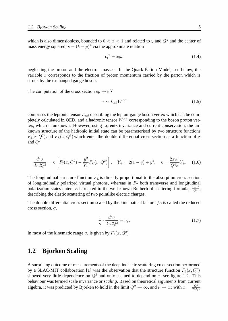
A surprising outcome of measurements of the deep inelastic scattering cross section performedby a SLAC-MIT collaboration [1] was the observation that the structure function F2(x, Q2)showed very little dependence on Q2 and only seemed to depend on x, see figure 1.2. Thisbehaviour was termed scale invariance or scaling. Based on theoretical arguments from currentalgebra, it was predicted by Bjorken to hold in the limit Q2 → ∞, and ν → ∞ with x = Q2
2Mpν
6 Chapter 1. Perturbative QCD and Deep Inelastic Scattering
Figure 1.2: Observation of scaling: Independence of the structure function νW2 =F2 of q2 = −Q2.The Bjorken variable x is kept fixed, x = 0.25.
kept fixed, where ν is the energy loss of the incoming lepton, ν = E−E ′, and Mp the rest massof the proton.
Scaling, the Q2 independence of the structure function F2 , suggested the existence of point-like scattering centers in the proton. That the proton itself was not a pointlike Dirac particlewas already known since the 1930s from the measurements of the anomalous magnetic momentof the proton [2], and later in the 1950s substantiated by the elastic electron proton scatteringexperiments by Hofstadter et al. [3].
The fact that the scattering target particle was not pointlike manifested itself in a suppression ofthe elastic electron proton scattering cross section, parameterised by a form factor, or structurefunction. This suppression is due to the destructive interference of partial waves scattered offsurface of an extended object, provided that the wavelength λ of the incoming particle streamis of the order of the spatial extension of the object.
1.3 Quark Parton Model
Feynman proposed a constituent model of the proton to consist of pointlike particles, calledpartons [4], which were readily identified with the quarks of the static quark model [5, 6]. Inthis model, called the Quark Parton Model, the cross section of deep inelastic ep scattering isexpressed as the incoherent sum of elementary elastic electron-parton scattering processes.
1.3. Quark Parton Model 7
The incoherence of these elastic scattering processes, i.e. neglecting the parton-parton interac-tions and treating them as quasi-free, is justified if the calculations are carried out in a framewhere the proton moves with infinite momentum. In this infinite momentum frame, the elec-tron parton scattering process can be shown to take place on a much shorter time scale as theparton-parton interactions.
The partons carry a certain fraction of the proton’s momentum which is identified with theBjorken scaling variable x. The number of partons dn of a certain flavour i encountered betweenan interval x and x + dx is parameterised by a parton distribution function fi(x), dn = f(x)dx.The momentum fraction dp of the protons momentum carried by these partons is then given bydp = xfi(x)dx.
The deep inelastic scattering cross section σep→eX , is thus given by convoluting the parton dis-tribution function with the (calculable) elastic electron parton cross sections σeqi→eqi
weightedby the electric charge ei of the parton and summed over all charged parton flavours i, denotedhere as qi:
(dσ
dxdQ2
)ep→eX
=∑
i
∫dx e2
i qi(x)
(dσ
dxdQ2
)eqi→eqi
. (1.8)
By equating formula 1.8 with 1.6, the Quark-Parton Master equation is obtained:
F2(x) =∑
i
e2i x [qi(x) + qi(x)] . (1.9)
The structure function F2 is thus seen to be independent of Q2 and related to the parton distri-bution functions of the proton.
The longitudinal structure function FL of equation 1.6 is related to the absorption cross sectionσL of longitudinally polarised virtual photons whereas F2 receives a transverse contribution σT
as well:
F2(x, Q2) =Q2
4π2α
(σT (x, Q2) + σL(x, Q2)
)(1.10)
FL(x, Q2) =Q2
4π2ασL(x, Q2). (1.11)
F2 and FL are related according to:
FL(x) = 2xF1(x) − F2(x) (1.12)
where F1(x) is a structure function similarly related purely to the absorbtion of transverselypolarized virtual photons.
Due to helicity and angular momentum conservation, and in the absence of intrinsic transversemomentum of the partons in the proton, longitudinally polarized virtual photons cannot beabsorbed by spin 1/2 partons, and thus, for spin 1/2 partons FL is predicted to be zero [7]. Forspin 0 partons, F1 would have been found to be zero. Experiments at SLAC confirmed the spin1/2 hypothesis [7].
8 Chapter 1. Perturbative QCD and Deep Inelastic Scattering
1.4 Quantum Chromodynamics
Soon after the SLAC experiment, violations of scaling were observed in muon nucleon scatter-ing [8] and later confirmed by neutrino nucleon scattering experiments [9]. The relation of F ν
2
to F μ,e2 confirmed the hypothesis of fractional quark charges. F2 was found to logarithmically
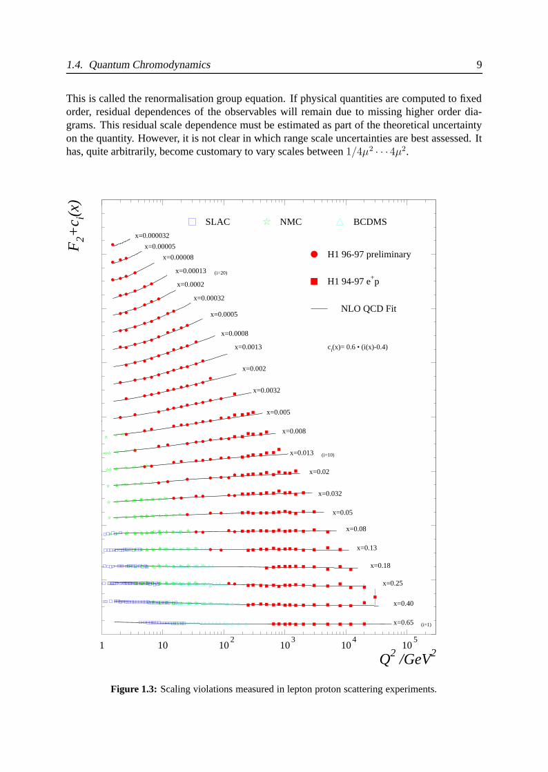
depend on Q2, see figure 1.3 for an overview. It shows the proton structure function F2 versusQ2 offset by a suitable constant for graphical representation. Scaling is seen to be violated atlow values of x, see figure 4.2, as well as high values of x, see figure 4.3. It is a fortunate coinci-dence that the SLAC measurements which established the Quark Parton Model were performedin the kinematic region of x 0.2 where scaling happens to be exact.
The ‘naive’ application of the Quark Parton Model was compromised not only by scaling vi-olations, but also by the fact that the quarks were found to carry only about 50% of the totalmomentum of the proton. These two observations were crucial in establishing QCD as thecorrect field theory of strong quark-gluon interactions.
1.4.1 The Running Coupling Constant
In gauge field theory, the strong interaction is mediated by mediator particles which could, asuncharged partons, account for the observed missing momentum in the proton. However, thefield theoretical description of deep inelastic scattering was long troubled by the fact that theQuark Parton Model assumption of quasi-free partons in the proton implied that the couplingstrength of the interaction be weak in the short-distance, high momentum transfer regime. Sinceno free quarks have been observed, however, the coupling strength on the other hand must berather large in the long distance, low momentum transfer regime, which leads to the confinementof quarks in hadrons. To account for these changes, the coupling strength seems to be varying(’running’) with the momentum transfer.
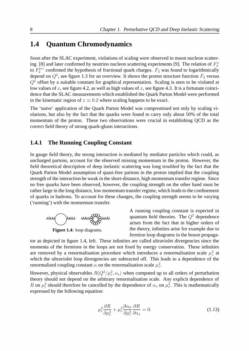
A running coupling constant is expected in
Figure 1.4: loop diagrams.
quantum field theories. The Q2 dependencearises from the fact that in higher orders ofthe theory, infinities arise for example due tofermion loop diagrams in the boson propaga-
tor as depicted in figure 1.4, left. These infinities are called ultraviolet divergencies since themomenta of the fermions in the loops are not fixed by energy conservation. These infinitiesare removed by a renormalisation procedure which introduces a renormalisation scale μ2
r atwhich the ultraviolet loop divergencies are subtracted off. This leads to a dependence of therenormalised coupling constant α on the renormalisation scale μ2
r.
However, physical observables R(Q2/μ2r, αs) when computed up to all orders of perturbation
theory should not depend on the arbitrary renormalisation scale. Any explicit dependence ofR on μ2
r should therefore be cancelled by the dependence of αs on μ2r. This is mathematically
expressed by the following equation:
μ2r
∂R
∂μ2r
+ μ2r
∂αS
∂μ2r
∂R
∂αs= 0. (1.13)
1.4. Quantum Chromodynamics 9
This is called the renormalisation group equation. If physical quantities are computed to fixedorder, residual dependences of the observables will remain due to missing higher order dia-grams. This residual scale dependence must be estimated as part of the theoretical uncertaintyon the quantity. However, it is not clear in which range scale uncertainties are best assessed. Ithas, quite arbitrarily, become customary to vary scales between 1/4μ2 · · · 4μ2.
1 10 102
103
104
105
x=0.65
x=0.40
x=0.25
x=0.18
x=0.13
x=0.08
x=0.05
x=0.032
x=0.02
x=0.013
x=0.008
x=0.005
x=0.0032
x=0.002
x=0.0013
x=0.0008
x=0.0005
x=0.00032
x=0.0002
x=0.00013
x=0.00008
x=0.00005
x=0.000032
(i=1)
(i=10)
(i=20)
Q2 /GeV2
F2+
c i(x)
NMC BCDMSSLAC
H1 94-97 e+p
H1 96-97 preliminary
NLO QCD Fit
ci(x)= 0.6 • (i(x)-0.4)
Figure 1.3: Scaling violations measured in lepton proton scattering experiments.
10 Chapter 1. Perturbative QCD and Deep Inelastic Scattering
In the case of QED, the loop diagrams effectively lead to vacuum polarisation due to virtuale+e− pairs which screen the bare charge e0 of a particle. At large distances or low momentumtransfer, the charge e seen by a probe is smaller than at short distances, or high momentumtransfer. Thus the coupling increases with increasing momentum transfer, a behaviour exactlyopposite to the behaviour observed in the case of the strong interaction.
The solution of this problem was found by observing that the correct gauge theory of stronginteraction is non-Abelian. In QCD, the degree of freedom connected to the interaction is thecolour charge which is carried by quarks and by the mediator particles, the gluons, alike. Thus,the gluons can couple to each other in contrast to the electrically neutral photons. This intro-duces additional loop diagrams depicted in figure 1.4, (right), which lead to an anti-screeningeffect.
The dependence of the strong coupling constant αs on the renormalisation scale can be com-puted by observing that the partial derivative ∂αs/∂μ2
r of equation 1.13 can itself be expressedin a power series of αs(μ
2r) and so-called β functions which are calculable in QCD:
μ2r
∂αs
∂μ2r
= αsβ(αS) = −β0α2
s
4π− β1
α3s
16π2+ ... . (1.14)
β0 = (33 − 2nf )/3
β1 = 102 − 38
3nf
where β0, β1 are the first coefficients occurring in the expansion and nf denoting the numberof active flavours, i.e. the quark flavours with masses smaller than μr.
In the one-loop approximation, i.e. regarding only the term with β0, the coupling constant αs
can be written in terms of the renormalization scale as
αs(μ2r) =
αs(μ20)
1 + b · αs(μ20) ln(μ2
r/μ20)
(1.15)
where b = β0/4π = (33 − 2nf)/12π and μ20 being a suitably chosen reference scale. The
presence of this scale μr is at the origin of scaling violations, as will be seen below.
The term −2nf/12π is due to the fermion loops and leads to screening effects similar as inQED. The term 33/12π gives rise to the antiscreening due to the gluon self-coupling: For lessthan 17 quark flavours, this is the dominating contribution and the coupling is seen to be fallingwith increasing μr, see figure 1.5. QCD is asymptotically free for Q2 → ∞, which is thereason why partons confined in the proton can be regarded as quasi-free as postulated in theQuark Parton Model. This property is unique to non-Abelian gauge theories. For Q2 → 0, thecoupling is seen to diverge. This can be viewed as a reason for the confinement of quarks andgluons inside hadrons. However, confinement is not really yet understood since the increase ofthe coupling constant prohibits the use of perturbation theory of the region of Q2 below a fewGeV2 .
1.4. Quantum Chromodynamics 11
Alternatively, the running of αs is often expressed as
αs(μ2r) =
1
b · ln(μ2r/Λ2
QCD), (1.16)
0.12
0.14
0.16
0.18
0.2
20 60 100 140 180Q [GeV)]
-0.005
0
0.005
0.01
0.015
0.02
0.025
0.03
20 60 100 140 180Q [GeV)]
αs(Q) for ΛMS=220 MeV:
1-loop2-loop3- and 4-loop
n = 1n = 2n = 3
αs[n-loop]
αs[4-loop]1− :
(a) (b)
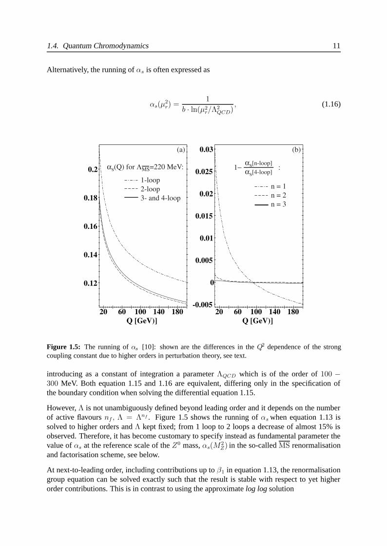
Figure 1.5: The running of αs [10]: shown are the differences in the Q2 dependence of the strongcoupling constant due to higher orders in perturbation theory, see text.
introducing as a constant of integration a parameter ΛQCD which is of the order of 100 −300 MeV. Both equation 1.15 and 1.16 are equivalent, differing only in the specification ofthe boundary condition when solving the differential equation 1.15.
However, Λ is not unambiguously defined beyond leading order and it depends on the numberof active flavours nf , Λ = Λnf . Figure 1.5 shows the running of αs when equation 1.13 issolved to higher orders and Λ kept fixed; from 1 loop to 2 loops a decrease of almost 15% isobserved. Therefore, it has become customary to specify instead as fundamental parameter thevalue of αs at the reference scale of the Z0 mass, αs(M
2Z) in the so-called MS renormalisation
and factorisation scheme, see below.
At next-to-leading order, including contributions up to β1 in equation 1.13, the renormalisationgroup equation can be solved exactly such that the result is stable with respect to yet higherorder contributions. This is in contrast to using the approximate log log solution
12 Chapter 1. Perturbative QCD and Deep Inelastic Scattering
αs(μ2r) =
1
b · ln(μ2r/Λ2
QCD)
[1 − b′
b
ln ln(μ2r/Λ2
QCD)
ln(μ2r/Λ2
QCD)
](1.17)
with b′ = β1/4πβ0. This approximation is sufficiently accurate for Q2 > m2c and used as a
convention adopted by [11]. In this analysis, the exact solution is employed and the differenceto αs obtained with the log log formula is quoted.
1.4.2 Factorisation
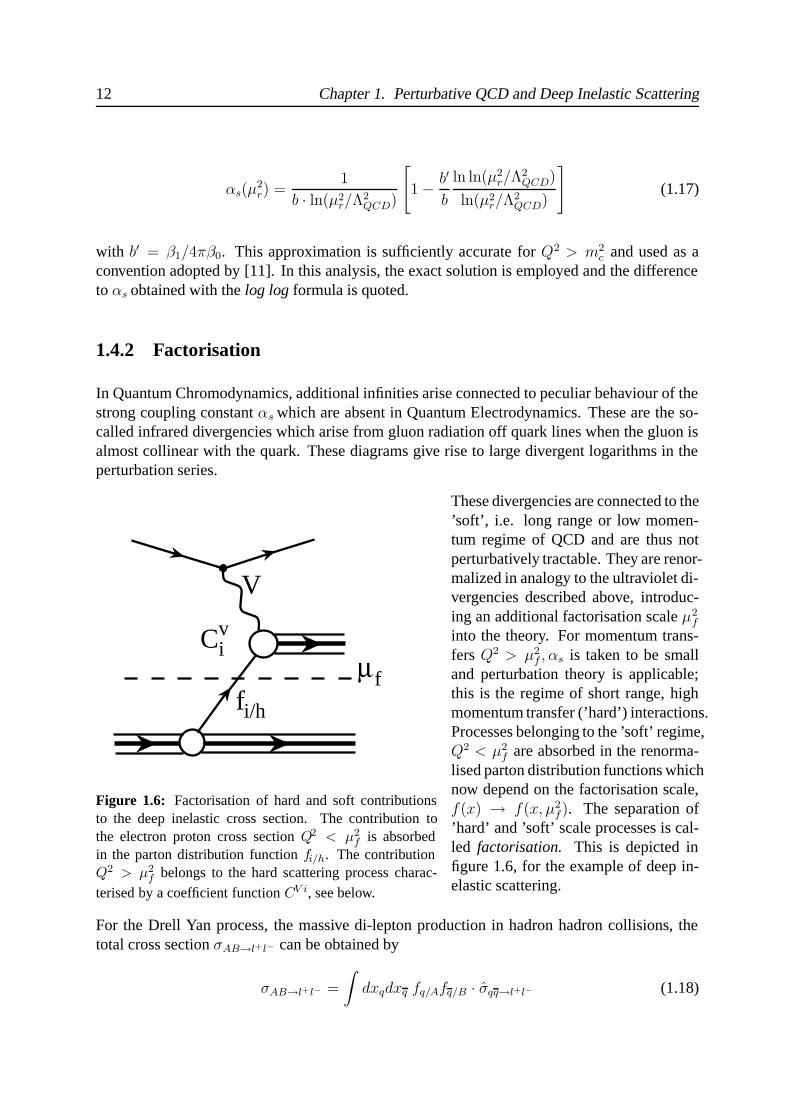
In Quantum Chromodynamics, additional infinities arise connected to peculiar behaviour of thestrong coupling constant αs which are absent in Quantum Electrodynamics. These are the so-called infrared divergencies which arise from gluon radiation off quark lines when the gluon isalmost collinear with the quark. These diagrams give rise to large divergent logarithms in theperturbation series.
These divergencies are connected to the
V
vCi
i/hffμ
Figure 1.6: Factorisation of hard and soft contributionsto the deep inelastic cross section. The contribution tothe electron proton cross section Q2 < μ2
f is absorbedin the parton distribution function fi/h. The contributionQ2 > μ2
f belongs to the hard scattering process charac-
terised by a coefficient function CV i, see below.
’soft’, i.e. long range or low momen-tum regime of QCD and are thus notperturbatively tractable. They are renor-malized in analogy to the ultraviolet di-vergencies described above, introduc-ing an additional factorisation scale μ2
f
into the theory. For momentum trans-fers Q2 > μ2
f , αs is taken to be smalland perturbation theory is applicable;this is the regime of short range, highmomentum transfer (’hard’) interactions.Processes belonging to the ’soft’ regime,Q2 < μ2
f are absorbed in the renorma-lised parton distribution functions whichnow depend on the factorisation scale,f(x) → f(x, μ2
f). The separation of’hard’ and ’soft’ scale processes is cal-led factorisation. This is depicted infigure 1.6, for the example of deep in-elastic scattering.
For the Drell Yan process, the massive di-lepton production in hadron hadron collisions, thetotal cross section σAB→l+l− can be obtained by
σAB→l+l− =
∫dxqdxq fq/Afq/B · σqq→l+l− (1.18)
1.4. Quantum Chromodynamics 13
It turns out that the collinear logarithmic divergencies connected to real and virtual gluon emis-sion which arise in Drell Yan di-lepton production are the same as in deep inelastic scattering.In fact it was proven by the factorisation theorems that this was a general feature of hard scat-tering processes in QCD [12]. As a consequence, the renormalised parton distribution functionsare universal and depend only on the hadron they belong to. Note that this corresponds to theassumptions made in the Quark Parton Model.
The differential cross sections for a reaction involving hadrons in the inital state can thus beobtained by convoluting the parton distribution functions f i/h of the respective hadron with thehard scattering cross section σ on the parton level.
1.4.3 F2 and FL in next-to-leading order QCD
For the process of deep inelastic scattering, the Quark Parton Model master equation 1.9 must bemodified by a factorisation scale dependent quark distribution functions. The scale μ2
f to whichhard and soft processes are compared to is usually taken to be Q2 but can also be provided bye.g. the transverse momentum p2
t or energy E2t or by a heavy quark mass m2
HQ.
With qi(x) → qi(x, μ2f = Q2) one thus obtains
F2(x, Q2) =∑
i
e2i x
[qi(x, Q2) + qi(x, Q2)
], (1.19)
i.e. F2 is now seen to be Q2 dependent and scale invariance is violated, albeit only logarithmi-cally as will be seen in the next sections.
Equation 1.19 is valid in the so-called leading log approximation, or in the DIS renormalisationand factorisation scheme to all orders, see below. At higher order, equation 1.19 is modified.Let us define for convenience
F2 =
nf∑i=1
e2i {qi + qi},
then F2 is computed in the next-to-leading order of the theory [13] as
F2
x=
(1 +
αs
2πC2
q
)⊗ F2(nf = 3) +
αs
2πC2
g ⊗( 3∑
f=1
e2f
)g +
F cc2
x(1.20)
.
F cc2 denotes the contribution of charm quarks which needs a separate treatment due to effects of
the heavy charm mass, see chapter 4.3. Cq and Cg denote the Wilson coefficients for quarks andgluons respectively which are known in perturbation theory to leading and next-to-leading order.Both F2 and F cc
2 are computed to order O(αs2) and the symbol ⊗ stands for the convolution:
f ⊗ g =
∫ 1
x
dz
zf(z)g(x/z).
14 Chapter 1. Perturbative QCD and Deep Inelastic Scattering
The coefficient functions in next-to-leading order are dependent on the factorisation and renor-malisation scheme due to the fact that there is freedom to choose how non-logarithmic longrange and short range contributions are absorbed in parton distributions and coefficient func-tions. In the DIS scheme, the coefficient functions are chosen such that equation 1.19 is validorder by order. Another conventional scheme is the MS [14] which follows from the idea ofdimensional regularisation [15]. In both schemes, μ2
f and μ2r are often taken to be equal and
fixed to Q2.
The proton structure function F2 in QCD can thus be expressed as a convolution of coefficientfunctions CV,i
2 which describe the perturbatively calculable interaction of the incoming leptonwith a parton of flavour i mediated by a gauge boson V and distributions of partons fi/h in thehadron h which have to be taken from experiment.
Similar expressions can be found for the longitudinal structure function FL . Note that there isa theoretical ambiguity as to which order O(αs ) F2 and FL are consistently calculated since inthe leading order of the theory FL =0, reproducing the Callan-Gross relation, equation 1.12.
The first non-vanishing order for FL is O(αs ) [16, 17]
FL
x=
αs
2πCL
q ⊗ F2 +αs
2πCL
g ⊗(∑
f
e2f
)g (1.21)
However, O(αs2) corrections on FL are sizable and this analysis employs consequently the
O(αs2) equations
FL
x=
(αs
2πCL
q +α2
s
(2π)2CL
2,NS
)⊗ F NS
2
+
(αs
2πCL
q +α2
s
(2π)2CL
2,S
)⊗ F S
2
+
(αs
2πCL
g +α2
s
(2π)2CL
2,g
)⊗
(∑f
e2f
)g (1.22)
F NS2 and F S
2 are functions of so-called non-singlet and singlet quark distribution functions,respectively, which will be discussed in the next section.
1.5 DGLAP Evolution and (∂F2/∂ ln Q2)x
Both F2 and FL are measurable quantities and thus should not depend on the choice of factorisa-tion scale μf . This requirement yields evolution equations for the parton distribution functionsfi(x, μ2
f) in which the structure functions decompose:
dfi(x, μ2f )
d lnμ2f
=αs(μ
2f)
2π
1∫x
dy
yfi(y, μ2
f)Pij(x/y) (1.23)
1.5. DGLAP Evolution and (∂F2/∂ ln Q2)x 15
This equation, known as the Dokshitzer, Gribov, Lipatov, Altarelli and Parisi (DGLAP [18])equation, is the analogue of the differential equation 1.15 describing the evolution of αs withμ2
r. In the following, μ2f is taken to be equal to Q2 for simplicity.
The functions Pij(x/y) are splitting functions calculable in perturbative QCD as a power seriesof αs(Q
2):
Pij(z, αs(Q2)) = δijP
(0)ij (z) +
αs
2πP
(1)ij (z) + ... (1.24)
They are known up to next-to-leading order, P (1). Calculations in next-to-NLO are under-way [19].
����Pqq
�x
y
�Pgq
�x
y
�Pqg
�x
y
�Pgg
�x
y
�(0) (0) (0) (0)
fj(y)
fi(x)
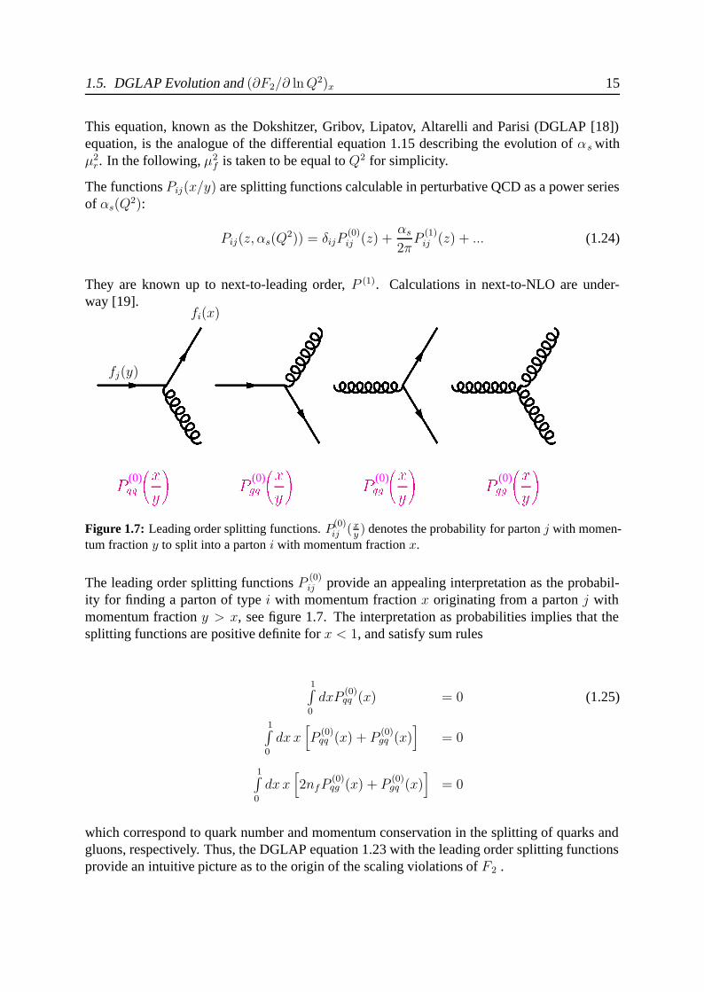
Figure 1.7: Leading order splitting functions. P(0)ij (x
y ) denotes the probability for parton j with momen-tum fraction y to split into a parton i with momentum fraction x.
The leading order splitting functions P(0)ij provide an appealing interpretation as the probabil-
ity for finding a parton of type i with momentum fraction x originating from a parton j withmomentum fraction y > x, see figure 1.7. The interpretation as probabilities implies that thesplitting functions are positive definite for x < 1, and satisfy sum rules
1∫0
dxP(0)qq (x) = 0 (1.25)
1∫0
dx x[P
(0)qq (x) + P
(0)gq (x)
]= 0
1∫0
dx x[2nfP
(0)qg (x) + P
(0)gq (x)
]= 0
which correspond to quark number and momentum conservation in the splitting of quarks andgluons, respectively. Thus, the DGLAP equation 1.23 with the leading order splitting functionsprovide an intuitive picture as to the origin of the scaling violations of F2 .
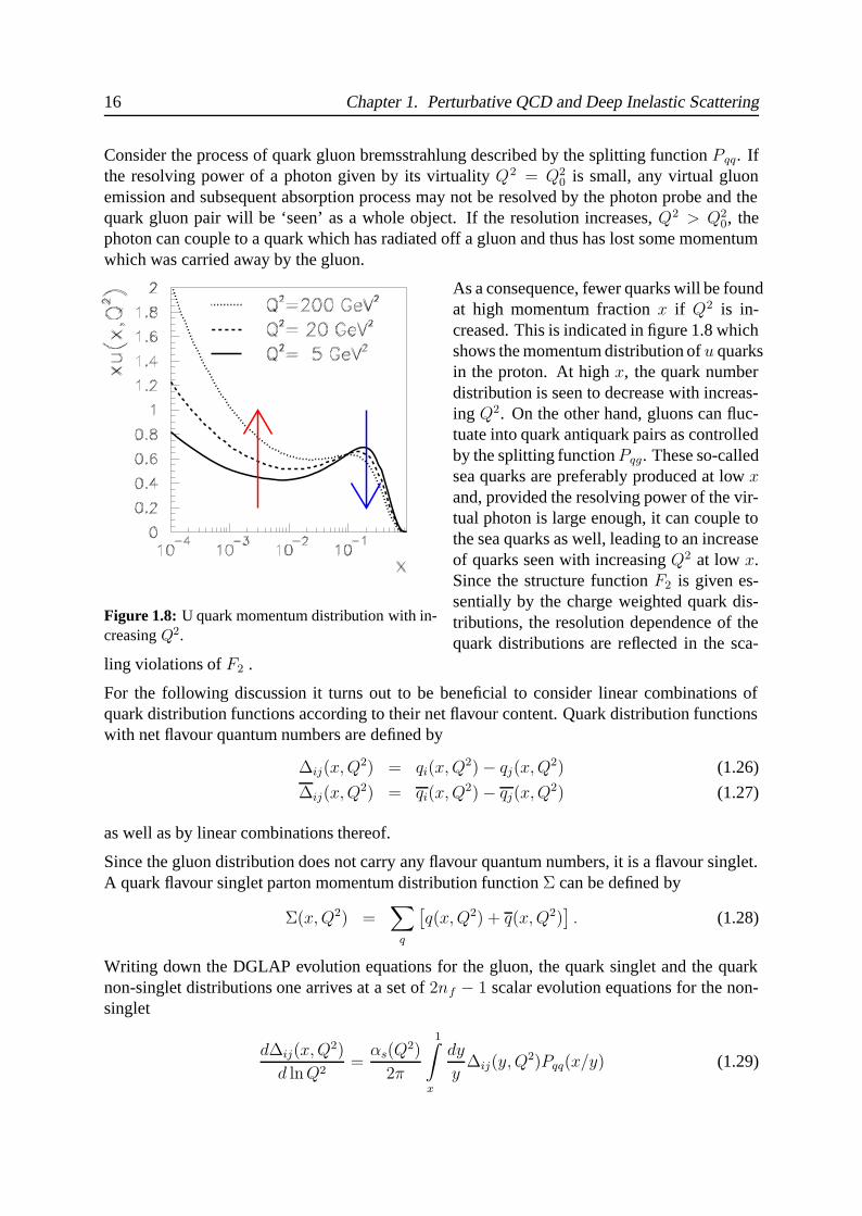
16 Chapter 1. Perturbative QCD and Deep Inelastic Scattering
Consider the process of quark gluon bremsstrahlung described by the splitting function Pqq. Ifthe resolving power of a photon given by its virtuality Q2 = Q2
0 is small, any virtual gluonemission and subsequent absorption process may not be resolved by the photon probe and thequark gluon pair will be ‘seen’ as a whole object. If the resolution increases, Q2 > Q2
0, thephoton can couple to a quark which has radiated off a gluon and thus has lost some momentumwhich was carried away by the gluon.
As a consequence, fewer quarks will be found
Figure 1.8: U quark momentum distribution with in-creasing Q2.
at high momentum fraction x if Q2 is in-creased. This is indicated in figure 1.8 whichshows the momentum distribution of u quarksin the proton. At high x, the quark numberdistribution is seen to decrease with increas-ing Q2. On the other hand, gluons can fluc-tuate into quark antiquark pairs as controlledby the splitting function Pqg. These so-calledsea quarks are preferably produced at low xand, provided the resolving power of the vir-tual photon is large enough, it can couple tothe sea quarks as well, leading to an increaseof quarks seen with increasing Q2 at low x.Since the structure function F2 is given es-sentially by the charge weighted quark dis-tributions, the resolution dependence of thequark distributions are reflected in the sca-
ling violations of F2 .
For the following discussion it turns out to be beneficial to consider linear combinations ofquark distribution functions according to their net flavour content. Quark distribution functionswith net flavour quantum numbers are defined by
Δij(x, Q2) = qi(x, Q2) − qj(x, Q2) (1.26)
Δij(x, Q2) = qi(x, Q2) − qj(x, Q2) (1.27)
as well as by linear combinations thereof.
Since the gluon distribution does not carry any flavour quantum numbers, it is a flavour singlet.A quark flavour singlet parton momentum distribution function Σ can be defined by
Σ(x, Q2) =∑
q
[q(x, Q2) + q(x, Q2)
]. (1.28)
Writing down the DGLAP evolution equations for the gluon, the quark singlet and the quarknon-singlet distributions one arrives at a set of 2nf − 1 scalar evolution equations for the non-singlet
dΔij(x, Q2)
d lnQ2=
αs(Q2)
2π
1∫x
dy
yΔij(y, Q2)Pqq(x/y) (1.29)
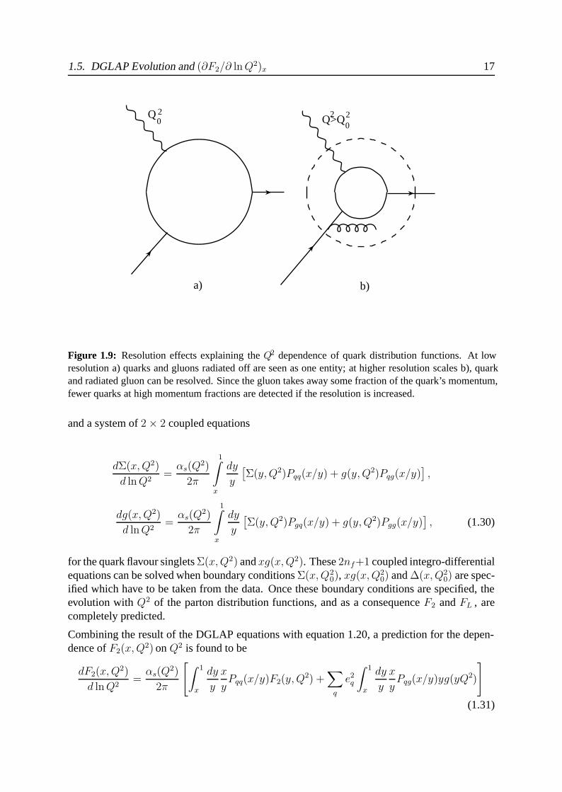
1.5. DGLAP Evolution and (∂F2/∂ ln Q2)x 17
Q>QQ 20 0
2
a) b)
2
Figure 1.9: Resolution effects explaining the Q2 dependence of quark distribution functions. At lowresolution a) quarks and gluons radiated off are seen as one entity; at higher resolution scales b), quarkand radiated gluon can be resolved. Since the gluon takes away some fraction of the quark’s momentum,fewer quarks at high momentum fractions are detected if the resolution is increased.
and a system of 2 × 2 coupled equations
dΣ(x, Q2)
d ln Q2=
αs(Q2)
2π
1∫x
dy
y
[Σ(y, Q2)Pqq(x/y) + g(y, Q2)Pqg(x/y)
],
dg(x, Q2)
d lnQ2=
αs(Q2)
2π
1∫x
dy
y
[Σ(y, Q2)Pgq(x/y) + g(y, Q2)Pgg(x/y)
], (1.30)
for the quark flavour singlets Σ(x, Q2) and xg(x, Q2). These 2nf+1 coupled integro-differentialequations can be solved when boundary conditions Σ(x, Q2
0), xg(x, Q20) and Δ(x, Q2
0) are spec-ified which have to be taken from the data. Once these boundary conditions are specified, theevolution with Q2 of the parton distribution functions, and as a consequence F2 and FL , arecompletely predicted.
Combining the result of the DGLAP equations with equation 1.20, a prediction for the depen-dence of F2(x, Q2) on Q2 is found to be
dF2(x, Q2)
d ln Q2=
αs(Q2)
2π
[∫ 1
x
dy
y
x
yPqq(x/y)F2(y, Q2) +
∑q
e2q
∫ 1
x
dy
y
x
yPqg(x/y)yg(yQ2)
]
(1.31)
18 Chapter 1. Perturbative QCD and Deep Inelastic Scattering
thus explaining the logarithmic scaling violations of F2(x, Q2) observed in figure 1.3 in theframework of QCD. The reason for the logarithmic dependence of the structure function on Q2
is the running of the coupling constant αs.
Note that the DGLAP equations do not give any x dependence of the parton distribution func-tions. The x dependence has to be entirely specified by the boundary conditions, taken fromoutside the theory. This is a consequence of the fact that the DGLAP evolution sums up theleading contribution which is coming from large logarithms ln Q2. In principle, an expansionhas to be performed in powers of
αps(ln Q2)q ln(1/x)r
In the leading order DGLAP theory, where ln Q2 is considered as the dominant contribution,p = q ≥ r ≥ 0. At NLO, terms for which p = q + 1 ≥ r ≥ 0 are summed as well. AtHERA, x is sufficiently small that the terms proportional to ln(1/x) should become importantand DGLAP be bound to fail; however, no such effect has so far been established. A search forsuch effects beyond DGLAP in inclusive scattering has been systematically performed in thisanalysis.
An important feature of the DGLAP evolution equations is the fact that the convolution integralsrun from x up to 1 rather than from 0 to 1. Thus, the theory provides predictions for the partondensities at higher momentum fraction y > x, independently of the knowledge of the partondistributions at momentum fractions smaller than x.
This allows the application of the QCD fit technique: parton distributions are parameterised atsome input scale Q2
0 , then they are evolved to higher values of Q2 and the theoretical predictionbased on the DGLAP evolution is tested against the data.
Chapter 2
An Accurate Cross Section Measurementat Low x
2.1 Extraction of the Cross Section
The deep inelastic cross section (equation 1.6) is measured double differentially in the Lorentzinvariant kinematic variables x and Q2. Measuring the cross section requires to basically countthe number of events N originating from DIS occuring in a bin, a certain region of x and Q2,�, and dividing this number by the luminosity L provided by the particle accelerator,
σ� = N/L. (2.1)
Of course, events from competing non-DIS processes give rise to a background contributionNBG in the bin which has to be identified and subtracted, N → N rec − NBG.
High energy physics experiments basically measure energy depositions in calorimeters andtracks in the detector’s tracking devices left by secondary particles produced in the hard inter-action. Thus, the Lorentz invariant variables must be reconstructed from the laboratory framemeasurements of particle energies and scattering angles.
In practice, these measurements suffer from imperfections of the detector: particles can escapedetection through acceptance holes such as cracks in the calorimeters, the geometry of thedetector or the beam pipe hole, due to detector inefficiencies (ε) and the like. Furthermore, thereconstructed variables xrec and Q2
rec are not to arbitrary precision identical to the true variablesof the hard interaction x and Q2 due to the finite resolution achieved by the detector in measuringangles and energies (smearing acceptance Acc). Also, radiative corrections (δrad) can lead tosystematic deviations of the measured from the ’true’ kinematic variables of the interaction atBorn level [20].
These effects lead to event migrations, N = N rec, which have to be accounted for in theextraction of the cross section (unfolding). Also, the effect of determining the cross sectiondiffentially in dxdQ2 by finite-sized bins � = ΔxΔQ2 adapted to the detector resolution hasto be accounted for (bin-center-correction Δbc).
19
20 Chapter 2. An Accurate Cross Section Measurement at Low x
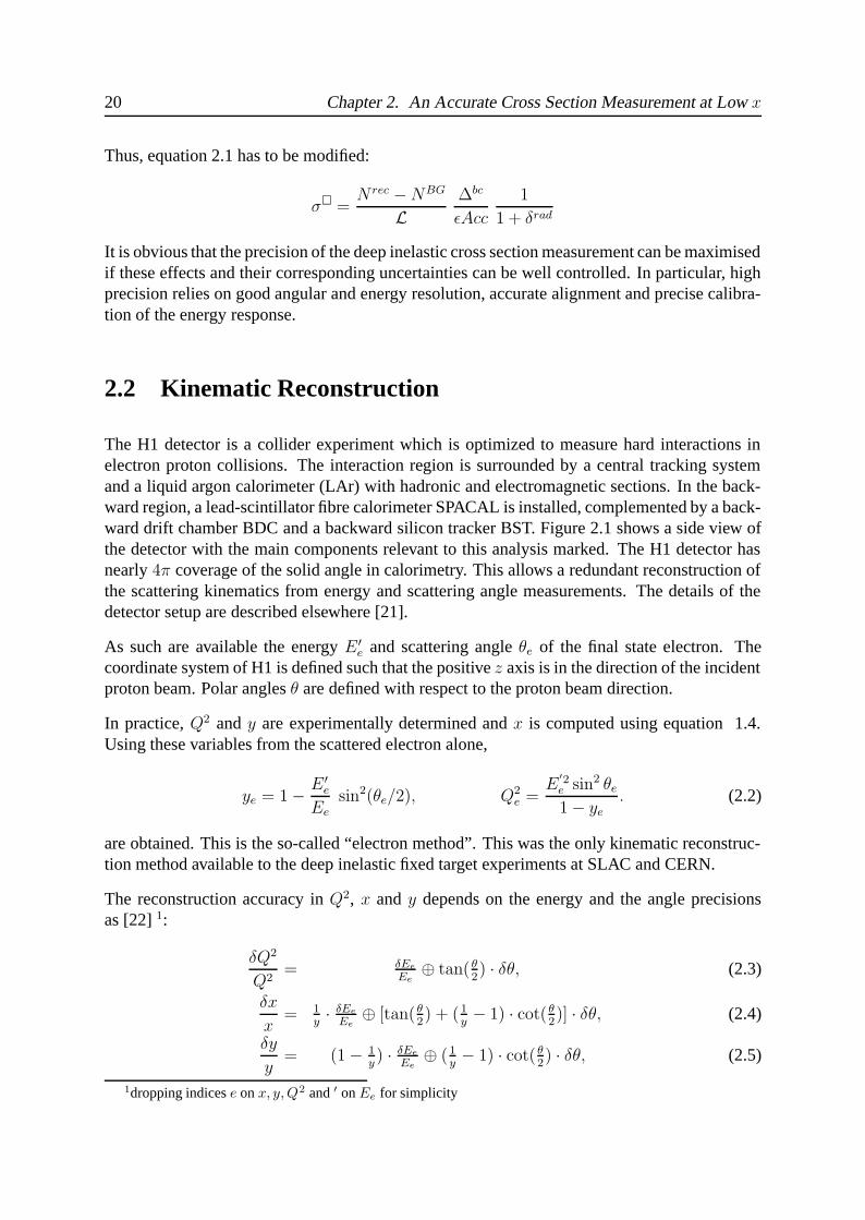
Thus, equation 2.1 has to be modified:
σ� =N rec − NBG
LΔbc
εAcc
1
1 + δrad
It is obvious that the precision of the deep inelastic cross section measurement can be maximisedif these effects and their corresponding uncertainties can be well controlled. In particular, highprecision relies on good angular and energy resolution, accurate alignment and precise calibra-tion of the energy response.
2.2 Kinematic Reconstruction
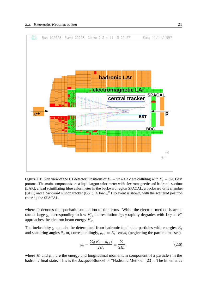
The H1 detector is a collider experiment which is optimized to measure hard interactions inelectron proton collisions. The interaction region is surrounded by a central tracking systemand a liquid argon calorimeter (LAr) with hadronic and electromagnetic sections. In the back-ward region, a lead-scintillator fibre calorimeter SPACAL is installed, complemented by a back-ward drift chamber BDC and a backward silicon tracker BST. Figure 2.1 shows a side view ofthe detector with the main components relevant to this analysis marked. The H1 detector hasnearly 4π coverage of the solid angle in calorimetry. This allows a redundant reconstruction ofthe scattering kinematics from energy and scattering angle measurements. The details of thedetector setup are described elsewhere [21].
As such are available the energy E ′e and scattering angle θe of the final state electron. The
coordinate system of H1 is defined such that the positive z axis is in the direction of the incidentproton beam. Polar angles θ are defined with respect to the proton beam direction.
In practice, Q2 and y are experimentally determined and x is computed using equation 1.4.Using these variables from the scattered electron alone,
ye = 1 − E ′e
Eesin2(θe/2), Q2
e =E
′2e sin2 θe
1 − ye. (2.2)
are obtained. This is the so-called “electron method”. This was the only kinematic reconstruc-tion method available to the deep inelastic fixed target experiments at SLAC and CERN.
The reconstruction accuracy in Q2, x and y depends on the energy and the angle precisionsas [22] 1:
δQ2
Q2= δEe
Ee⊕ tan( θ
2) · δθ, (2.3)
δx
x= 1
y· δEe
Ee⊕ [tan( θ
2) + ( 1
y− 1) · cot( θ
2)] · δθ, (2.4)
δy
y= (1 − 1
y) · δEe
Ee⊕ ( 1
y− 1) · cot( θ
2) · δθ, (2.5)
1dropping indices e on x, y, Q2 and ′ on Ee for simplicity
2.2. Kinematic Reconstruction 21
hadronic LAr
electromagnetic LAr
BST
central tracker
BDC
SPACAL
pe+
Figure 2.1: Side view of the H1 detector. Positrons of Ee = 27.5 GeV are colliding with Ep = 820 GeVprotons. The main components are a liquid argon calorimeter with electromagnetic and hadronic sections(LAR), a lead scintillating fibre calorimeter in the backward region SPACAL, a backward drift chamber(BDC) and a backward silicon tracker (BST). A low Q2 DIS event is shown, with the scattered positronentering the SPACAL.
where ⊕ denotes the quadratic summation of the terms. While the electron method is accu-rate at large y, corresponding to low E ′
e, the resolution δy/y rapidly degrades with 1/y as E ′e
approaches the electron beam energy Ee.
The inelasticity y can also be determined from hadronic final state particles with energies Ei
and scattering angles θi, or, correspondingly, pz,i = Ei · cos θi (neglecting the particle masses).
yh =Σi(Ei − pz,i)
2Ee
≡ Σ
2Ee
, (2.6)
where Ei and pz,i are the energy and longitudinal momentum component of a particle i in thehadronic final state. This is the Jacquet-Blondel or “Hadronic Method” [23] . The kinematics
22 Chapter 2. An Accurate Cross Section Measurement at Low x
can also be reconstructed with the “Σ method” using the variables [24]
yΣ =Σ
Σ + E ′e(1 − cos θe)
, Q2Σ =
E′2e sin2 θe
1 − yΣ
. (2.7)
The hadronic variables yh and yΣ are related according to
yΣ =yh
1 + yh − ye
(2.8)
and can be well measured down to low y 0.004.
The variable yΣ is less sensitive to initial state radiation than yh since the initial energy Ee inthe denominator in equation 2.6 can be calculated using the total energy reconstructed in thedetector which leads to equation 2.7. The precision of this method depends on the calorimetersampling fluctuations which become important at low Pt,h, where Pt,h is the total transversemomentum of the hadronic final state particles. The resolution δyh/yh degrades ∝ 1/(1 − y),limiting the hadron method to low values of y.
Thus, the electron method and the hadronic method complement one another and extend to dif-ferent regions of phase space. For the data analysis described in the next section, the kinematicreconstruction by means of the electron method is used for values y > 0.15, and for lowervalues the hadronic method is employed.
The redundancy of the kinematic reconstruction allow yet another method to be used basedon angle measurements only. From the hadronic final state particles, an effective hadronicscattering angle θh can be derived which is defined as
tanθh
2=
Σ
Pt,h, (2.9)
In the naive quark parton model, θh defines the direction of the struck quark related to θe as
tanθh
2=
y
1 − y· tan
θe
2. (2.10)
This relation, together with the definition of ye (equation 2.2), determines the scattered electronenergy from θe and θh in the “double angle method” [25]. This method is essential for calibra-tion purposes since the energy response of the detector can be compared to the double angleprediction.
2.3 Data Analysis with the H1 Detector
2.3.1 Datasets
In this work, datasets on the deep inelastic neutral current scattering cross section were analysedtaken by the H1 collaboration in 1996 and 1997.
The data were taken in different samples:
2.3. Data Analysis with the H1 Detector 23
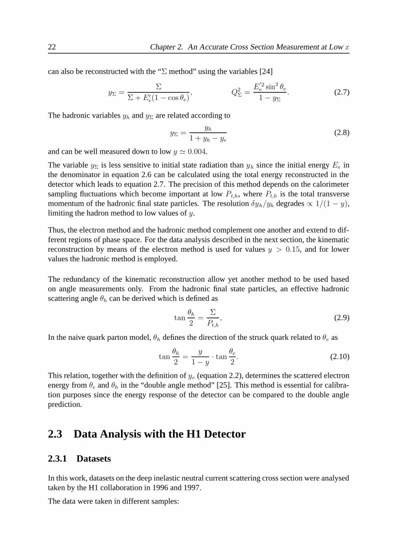
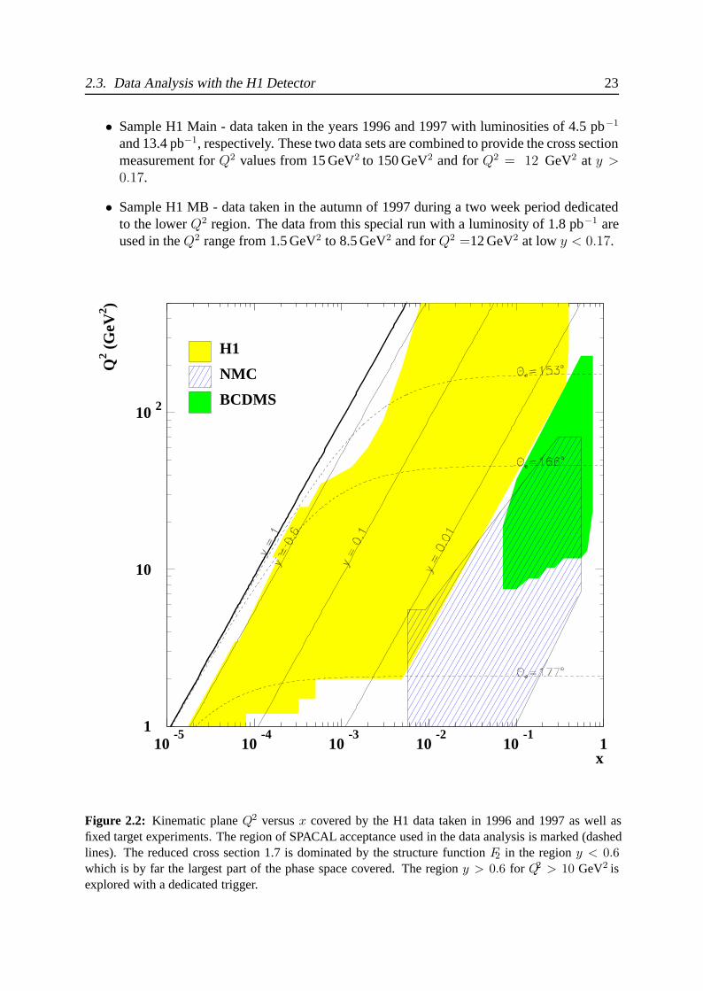
• Sample H1 Main - data taken in the years 1996 and 1997 with luminosities of 4.5 pb−1
and 13.4 pb−1, respectively. These two data sets are combined to provide the cross sectionmeasurement for Q2 values from 15 GeV2 to 150 GeV2 and for Q2 = 12 GeV2 at y >0.17.
• Sample H1 MB - data taken in the autumn of 1997 during a two week period dedicatedto the lower Q2 region. The data from this special run with a luminosity of 1.8 pb−1 areused in the Q2 range from 1.5 GeV2 to 8.5 GeV2 and for Q2 =12 GeV2 at low y < 0.17.
1
10
10 2
10-5
10-4
10-3
10-2
10-1
1x
Q2 (
GeV
2 )
BCDMS
NMC
H1
Figure 2.2: Kinematic plane Q2 versus x covered by the H1 data taken in 1996 and 1997 as well asfixed target experiments. The region of SPACAL acceptance used in the data analysis is marked (dashedlines). The reduced cross section 1.7 is dominated by the structure function F2 in the region y < 0.6which is by far the largest part of the phase space covered. The region y > 0.6 for Q2 > 10 GeV2 isexplored with a dedicated trigger.
24 Chapter 2. An Accurate Cross Section Measurement at Low x
These datasets cover a region in 1.5 < Q2 < 150 GeV2 and 3 · 10−5 < x < 0.25 depictedin figure 2.2. Values of the inelasticity y > 0.8 were achieved for Q2 > 12 GeV2 in a separateanalysis based on a dedicated trigger sample with luminosities of 2.8 pb−1 obtained 1996 and3.4 pb−1 in 1997 [26, 27].
The data analysis of this work was performed on the H1 MAIN and H1 MB data samples inthe kinematic region y < 0.8. The results on the extracted double differential cross sectionmeasurement from the H1 MAIN dataset for y < 0.15 (Σ method) and the results from the H1MB for y > 0.15 (electron method), limited to y < 0.6 for Q2 < 5 GeV2 , were publishedin [27].
2.3.2 Event Selection Strategy
DIS events at low Q2 are identified with the final state electrons scattered in the backwardcalorimeter SPACAL of the H1 detector, covering scattering angles of (153◦ < θe < 177◦).According to equation 2.7, this limits the measurement to Q2 < 150 GeV2 .
This calorimeter is a lead-fibre spaghetti calorimeter with high energy resolution [28]
σE
E=
7.5%√E[GeV ]
⊕ 1%
and high transverse granularity. This allows an accurate energy measurement of the scatteredelectron as well as the distinction of electromagnetic from hadronic energy deposits by meansof their respective lateral shower profile.
Electromagnetic energy deposits by neutral particles can be removed by requiring a signal in thetrack detectors in front of the calorimeter. Tracks of charged final state particles are recordedin the central track detector which allows to reconstruct the primary vertex of the interaction.Beam related background can thus be removed [29].
Longitudinal momentum conservation in neutral current DIS events constrains the variable E−pz, summed over the final state particles,
E − pz = Σ + E ′e(1 − cos θe) (2.11)
to be approximately equal to 2Ee. In radiative events a photon may carry a significant fractionof the E − pz sum. These events can be removed from the data sample by a suitable cut onE − pz.
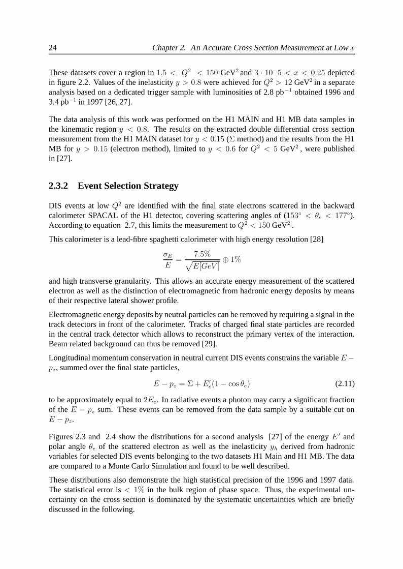
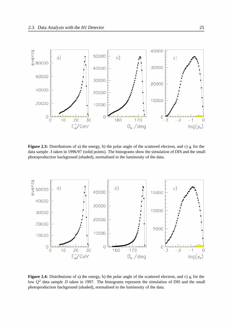
Figures 2.3 and 2.4 show the distributions for a second analysis [27] of the energy E ′ andpolar angle θe of the scattered electron as well as the inelasticity yh derived from hadronicvariables for selected DIS events belonging to the two datasets H1 Main and H1 MB. The dataare compared to a Monte Carlo Simulation and found to be well described.
These distributions also demonstrate the high statistical precision of the 1996 and 1997 data.The statistical error is < 1% in the bulk region of phase space. Thus, the experimental un-certainty on the cross section is dominated by the systematic uncertainties which are brieflydiscussed in the following.
2.3. Data Analysis with the H1 Detector 25
´
Figure 2.3: Distributions of a) the energy, b) the polar angle of the scattered electron, and c) yh for thedata sample A taken in 1996/97 (solid points). The histograms show the simulation of DIS and the smallphotoproduction background (shaded), normalised to the luminosity of the data.
´
Figure 2.4: Distributions of a) the energy, b) the polar angle of the scattered electron, and c) yh for thelow Q2 data sample B taken in 1997. The histograms represent the simulation of DIS and the smallphotoproduction background (shaded), normalised to the luminosity of the data.
26 Chapter 2. An Accurate Cross Section Measurement at Low x
2.3.3 Electromagnetic Energy Calibration
At low Q2 the DIS events exhibit an accumulation at E ′e about the electron beam energy which
is called the kinematic peak. This kinematic peculiarity serves as a high quality measure ofthe accuracy of the electromagnetic energy scale [30]. By using the energy reference scaleprovided by the double angle method, the calibration of the backward detector can be furtherimproved [31] and resolution effects be understood.
The electromagnetic energy scale is accurate up to about 0.5% at high energies E ′e ∼ Ee and is
known to be less precise ∼ 3% at lower energies. This can be determined with QED Comptonevents [32, 33, 34].
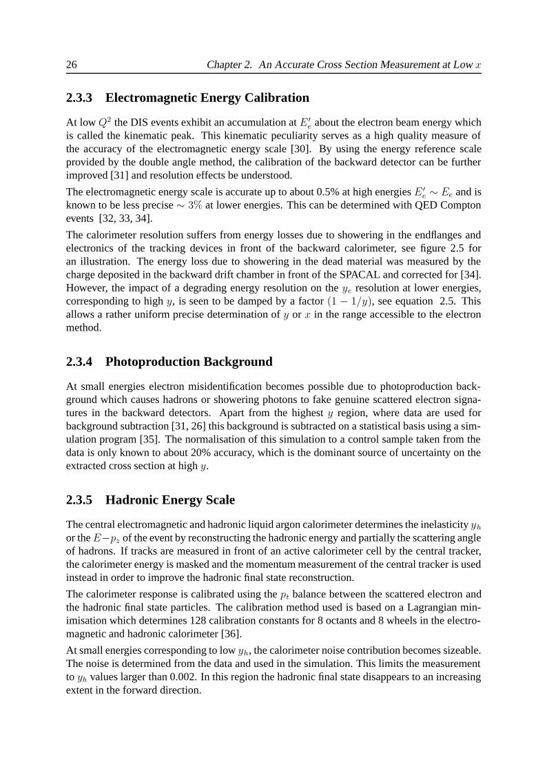
The calorimeter resolution suffers from energy losses due to showering in the endflanges andelectronics of the tracking devices in front of the backward calorimeter, see figure 2.5 foran illustration. The energy loss due to showering in the dead material was measured by thecharge deposited in the backward drift chamber in front of the SPACAL and corrected for [34].However, the impact of a degrading energy resolution on the ye resolution at lower energies,corresponding to high y, is seen to be damped by a factor (1 − 1/y), see equation 2.5. Thisallows a rather uniform precise determination of y or x in the range accessible to the electronmethod.
2.3.4 Photoproduction Background
At small energies electron misidentification becomes possible due to photoproduction back-ground which causes hadrons or showering photons to fake genuine scattered electron signa-tures in the backward detectors. Apart from the highest y region, where data are used forbackground subtraction [31, 26] this background is subtracted on a statistical basis using a sim-ulation program [35]. The normalisation of this simulation to a control sample taken from thedata is only known to about 20% accuracy, which is the dominant source of uncertainty on theextracted cross section at high y.
2.3.5 Hadronic Energy Scale
The central electromagnetic and hadronic liquid argon calorimeter determines the inelasticity yh
or the E−pz of the event by reconstructing the hadronic energy and partially the scattering angleof hadrons. If tracks are measured in front of an active calorimeter cell by the central tracker,the calorimeter energy is masked and the momentum measurement of the central tracker is usedinstead in order to improve the hadronic final state reconstruction.
The calorimeter response is calibrated using the pt balance between the scattered electron andthe hadronic final state particles. The calibration method used is based on a Lagrangian min-imisation which determines 128 calibration constants for 8 octants and 8 wheels in the electro-magnetic and hadronic calorimeter [36].
At small energies corresponding to low yh, the calorimeter noise contribution becomes sizeable.The noise is determined from the data and used in the simulation. This limits the measurementto yh values larger than 0.002. In this region the hadronic final state disappears to an increasingextent in the forward direction.
2.3. Data Analysis with the H1 Detector 27
x [cm]
y [c
m]
-80
-60
-40
-20
0
20
40
60
80
-80 -60 -40 -20 0 20 40 60 80
Figure 2.5: Visualisation of the dead material in front of the backward calorimeter SPACAL. Shownis the mean charge measured in the backward chamber in arbitrary units. Darker colours indicate highcharge deposits. The most prominent 16 fold structure is due to readout electronics for the central innerproportional chamber CIP which is part of the central tracker of H1.
28 Chapter 2. An Accurate Cross Section Measurement at Low x
2.4 Systematic Errors
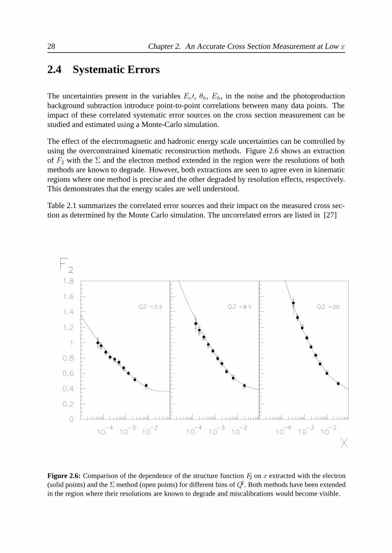
The uncertainties present in the variables Ee′, θh, Eh, in the noise and the photoproductionbackground subtraction introduce point-to-point correlations between many data points. Theimpact of these correlated systematic error sources on the cross section measurement can bestudied and estimated using a Monte-Carlo simulation.
The effect of the electromagnetic and hadronic energy scale uncertainties can be controlled byusing the overconstrained kinematic reconstruction methods. Figure 2.6 shows an extractionof F2 with the Σ and the electron method extended in the region were the resolutions of bothmethods are known to degrade. However, both extractions are seen to agree even in kinematicregions where one method is precise and the other degraded by resolution effects, respectively.This demonstrates that the energy scales are well understood.
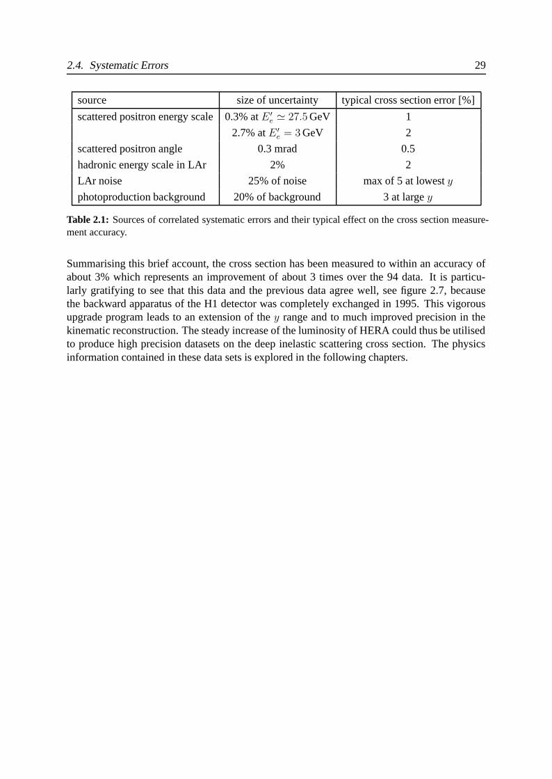
Table 2.1 summarizes the correlated error sources and their impact on the measured cross sec-tion as determined by the Monte Carlo simulation. The uncorrelated errors are listed in [27]
Figure 2.6: Comparison of the dependence of the structure function F2 on x extracted with the electron(solid points) and the Σ method (open points) for different bins of Q2. Both methods have been extendedin the region where their resolutions are known to degrade and miscalibrations would become visible.
2.4. Systematic Errors 29
source size of uncertainty typical cross section error [%]
scattered positron energy scale 0.3% at E ′e 27.5 GeV 1
2.7% at E ′e = 3 GeV 2
scattered positron angle 0.3 mrad 0.5
hadronic energy scale in LAr 2% 2
LAr noise 25% of noise max of 5 at lowest y
photoproduction background 20% of background 3 at large y
Table 2.1: Sources of correlated systematic errors and their typical effect on the cross section measure-ment accuracy.
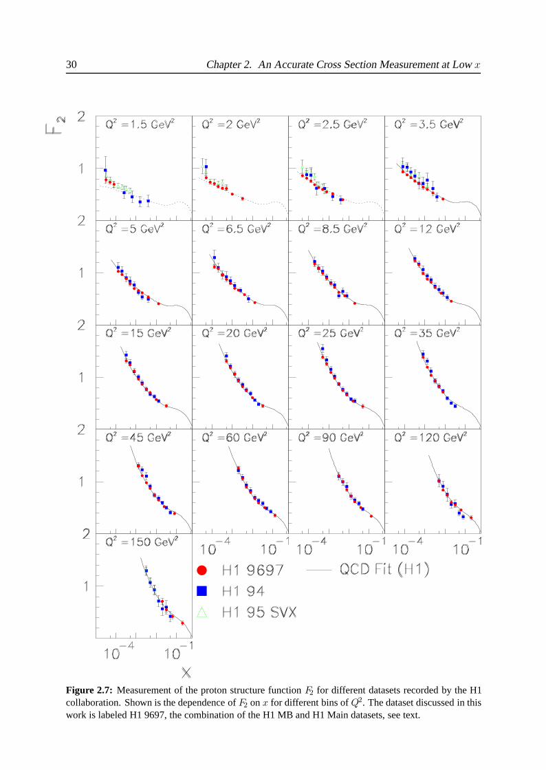
Summarising this brief account, the cross section has been measured to within an accuracy ofabout 3% which represents an improvement of about 3 times over the 94 data. It is particu-larly gratifying to see that this data and the previous data agree well, see figure 2.7, becausethe backward apparatus of the H1 detector was completely exchanged in 1995. This vigorousupgrade program leads to an extension of the y range and to much improved precision in thekinematic reconstruction. The steady increase of the luminosity of HERA could thus be utilisedto produce high precision datasets on the deep inelastic scattering cross section. The physicsinformation contained in these data sets is explored in the following chapters.
30 Chapter 2. An Accurate Cross Section Measurement at Low x
Figure 2.7: Measurement of the proton structure function F2 for different datasets recorded by the H1collaboration. Shown is the dependence of F2 on x for different bins of Q2. The dataset discussed in thiswork is labeled H1 9697, the combination of the H1 MB and H1 Main datasets, see text.
Chapter 3
QCD Analysis Procedure
The accuracy of the inclusive cross section measurement at low x and Q2 reached by the H1experiment has allowed to perform a first simultaneous determination of the strong couplingconstant αs and of the gluon momentum distribution xg at low x. This requires an extremelycareful QCD analysis to be performed which is the main goal of this work.
The predictions of the QCD evolution equations 1.29 and 1.30 are confronted with the reduceddifferential cross section measurements of the H1 low Q2 data, discussed in the previous chap-ter, as well as with recent H1 data at high Q2 ≥ 150 GeV2 [37] from the same data takingperiod.
The guiding principles of the analysis are a use of a minimal number of datasets and fit pa-rameters alongside a maximal exploitation of experimental knowledge on the uncertainties ofthe data with full error propagation to the determined values of αs and xg . They therefore arecomplementary to the procedure applied in global fits [38, 39, 40] which aim for an almostcomplete determination of all parton momentum distribution functions in the nucleon using amaximum amount of available data. Global analyses have to address questions on the consis-tency of the various datasets [41] and have to deal with quite challenging error propagationproblems [42, 43].
3.1 Analysis Procedure
3.1.1 Singlet and Non-Singlet Evolution of F2
The gluon xg and quark flavour singlet Σ distributions are dynamically coupled via the DGLAPequations 1.30 whereas quark flavour non-singlets evolve independently of xg [44]. Solving theevolution equations thus requires to specify the gluon, singlet and non-singlet parton momentumdistribution functions as boundary conditions at an input scale Q2
0 .
It is instructive to identify the singlet and non-singlet contributions to F2 in the leading orderQCD formalism with Q2 dependent quark distribution functions. In the quark-parton model, theproton structure function F2 is given by a sum of quark and anti-quark momentum distribution
31
32 Chapter 3. QCD Analysis Procedure
functions, see equation 1.19. The flavour singlet parton momentum distribution function Σ isgiven as
Σ(x, Q2) =∑
q
[q(x, Q2) + q(x, Q2)
]. (3.1)
Flavour non-singlet parton momentum distribution functions can be defined as
Δij(x, Q2) = qi(x, Q2) − qj(x, Q2) (3.2)
Δij(x, Q2) = qi(x, Q2) − qj(x, Q2) (3.3)
as well as linear combinations thereof.
For simplicity, consider a four quark flavour model with massless (u, d, s, c) quarks, and letU = u + u + c + c and D = d + d + s + s, where the functional dependence on (x, Q2) isimplied but suppressed for clarity in the following. Then, the quark flavour singlet functionis given as Σ = U + D, while Δ = U − D defines a flavour non-singlet quark distributionfunction, yielding the decompositions
F2 =4
9xU +
1
9xD (3.4)
F2 =5
18xΣ +
1
6xΔ (3.5)
for the proton structure function F2 . Thus, F2 is determined by two independent combinationsof quark distribution functions which define the singlet and non-singlet sector of the DGLAPequations.
Traditionally, QCD analyses based on the DGLAP equations make use of both lepton-protonand lepton-deuteron data [45, 46, 47, 48, 49] in order to separate the non-singlet and singletevolution, and also to determine the parton distributions of up and down quarks simultaneously.This can be illustrated as follows.
Invoking isospin symmetry, the deuteron structure function F d2 , disregarding nuclear correc-
tions, is given as
F d2 =
5
18xΣ +
1
6
(Δ − Δ+
)(3.6)
with Δ+ = (u + u)− (d + d) defining an additional non-singlet parton momentum distributionfunction which is sensitive to the up and down quark distribution functions. Assuming anisospin symmetric up and down quark sea, one obtains Δ+ = uv − dv which represents anotherconstraint on the valence quark distributions. In such fits, the quark counting rules can thereforeseparately be enforced on the valence up and down quark distributions.
Furthermore, since Δ+ = Δ− (c + c)+ (s + s), it can be seen that F d2 is an almost pure singlet
function apart from a small charm and strange quark sea contribution. By adding deuteronand proton structure function data in the fit, the singlet and non-singlet dynamics can thus beseparated.
3.1. Analysis Procedure 33
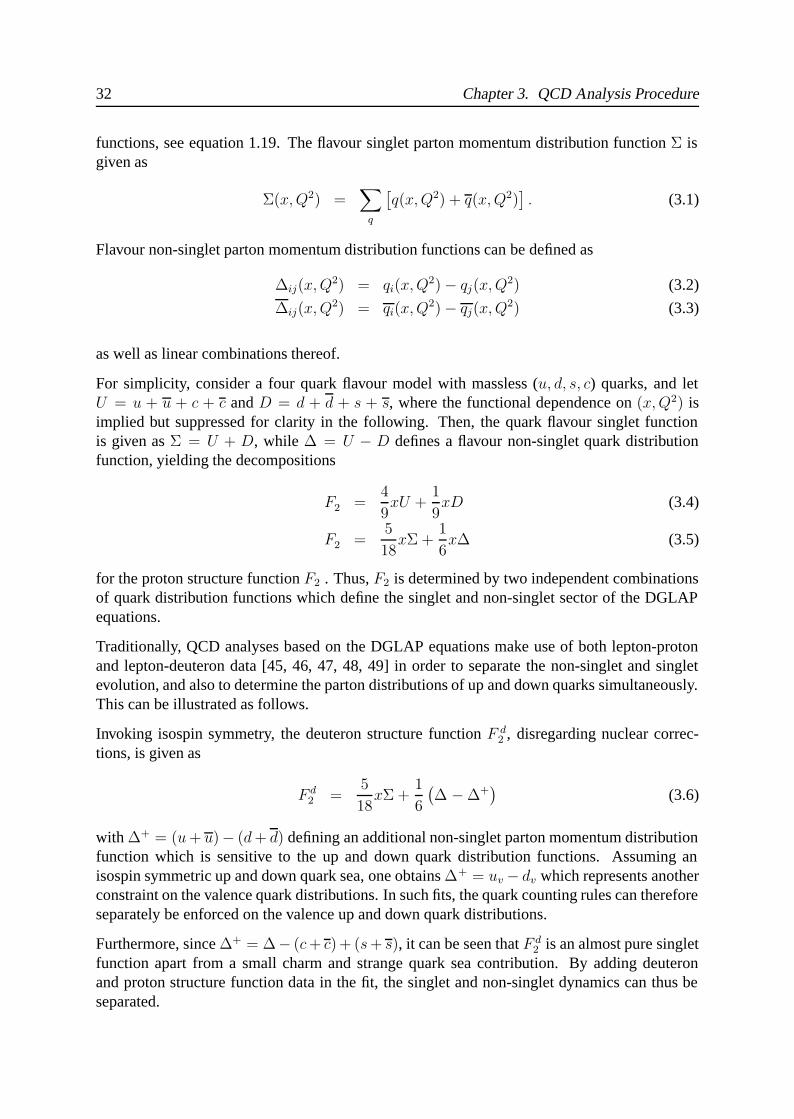
Since precise data over a wide (Q2, x) range are now available, however, which represent astrong constraint on the evolution of Σ, Δ and xg , a QCD analysis without using deuteron datais attempted here. This will not lead to flavour separated parton distribution, but it will be shownto be adequate to the goal of measuring αs and xg . A notable advantage of such an approachis its independence of corrections for nuclear binding effects in the deuteron (shadowing, targetmass and Fermi motion). These corrections imply an additional uncertainty to the fit results dueto the use of nuclear models [50, 51]. Furthermore, the constraint of the present data on the uand d quark distributions is still limited in the valence region, see figure 3.1.
Figure 3.1: The ratio of the up and down quark distribution and its uncertainty. At high x, d/u isessentially still undetermined [47].
34 Chapter 3. QCD Analysis Procedure
3.2 Flavour Decomposition
In this analysis, an attempt is made to use proton target data only. Thus the up and downvalence quark distributions cannot be disentangled, but the valence quark counting rules maystill be applied to an effective valence quark distribution. This requires a suitably chosen flavourdecomposition of F2 in singlet and non-singlet quark distributions.
3.2.1 Simplified Ansatz
In the present analysis, the sum in equation 1.19 extends only over up, down and strange(u, d, s) quarks. The charm and beauty contributions are treated differently due to heavy quarkmass effects, see chapter 4. At low x, about 20% of the inclusive cross section is due to charmproduction, dominated by the photon-gluon fusion process, whereas the beauty contribution isless then 1 %. These heavy flavour contributions are added using NLO QCD calculations [52]in the on-mass shell renormalisation scheme using mc = 1.4 GeV and mb = 4.5 GeV.
For the three light flavours, F2 then decomposes in singlet and non-singlet quark distributionsas
F2 =2
9· xΣ +
1
3· xΔ (3.7)
with Δ = (2U − D)/3 defining a non-singlet distribution.
Now a suitable projection of F2 into two independent quark distribution functions V and A whichallow the use of the valence quark counting rule is found according to
F2 =1
3xV +
11
9xA. (3.8)
Assuming for simplicity s + s = 12(u + d), the functions V and A are related to the uptype
U = u + u and downtype D = d + d + s + s quark distributions as
U =2
3V + 2A (3.9)
and
D =1
3V + 3A. (3.10)
The inverse relations defining V and A are
V =3
4(3U − 2D) =
9
4uv − 3
2dv +
9
2u − 3(d + s)
u=d−→ 3
4(3uv − 2dv) (3.11)
and
A =1
4(2D − U) = d + s − 1
2u − 1
4uv +
1
2dv
u=d−→ u − 1
4(uv − 2dv). (3.12)
3.2. Flavour Decomposition 35
Assuming roughly uv = 2dv for illustration one finds V ≈ 32uv and A ≈ u, i.e. V defines
a valence type distribution while A is dominated by the sea quarks and determines the low xbehaviour of F2 .
An advantage of this decomposition is that V is constrained by the relation
∫ 1
0
V dx = 3, (3.13)
i.e. although only proton target data are used the quark counting rule can be employed. Anotherconstraint is provided by the momentum sum rule
∫ 1
0
(xg + Σ) dx = 1. (3.14)
This ansatz is generalised in the following section to account for the observed small deviationsof the strange [53] and antiquark [54] distributions from the conventional assumptions aboutthe sea.
3.2.2 Generalised Flavour Decomposition of F2
Recent measurements of Drell-Yan muon pair production at the Tevatron [54] have establisheda difference between the u and d distributions which was first observed in [55]. Charged currentneutrino-nucleon experiments determined the relative amount of strange quarks in the nucleonsea to be
s + s = (1
2+ ε) · (u + d), (3.15)
with a recent value of ε = −0.08 [56]. The evolution of s + s in DGLAP QCD is found toyield a linear dependence of ε on ln Q2 which is used to extrapolate the NuTeV result obtainedat 16 GeV2 , to Q2 = Q2
0. Both results have been accounted for by modifying equation 3.10according to
D =1
3V + kA, (3.16)
which, using equation 3.9, results in
V =3
2· 1
k − 1(kU − 2D) (3.17)
and Σ = V +A · (2+k). Choosing k = 3+2ε can be shown to remove the strange contributionto the function V yielding
V =3
4· 1
1 + ε[(3 + 2ε)uV − 2dV + (5 + 2ε)(u − d)], (3.18)
36 Chapter 3. QCD Analysis Procedure
which coincides with equation 3.11 for ε = 0 and u = d. Because the integral δ =∫
(u − d)dxis finite 1, this choice of k allows the counting rule constraint (equation 3.13) to be maintainedas ∫ 1
0
V dx = 3 + δ · 3
4· 5 + 2ε
1 + ε= v(ε, δ). (3.19)
If this constraint is released in a fit to the H1 data, a value of∫
V dx = 2.24 ± 0.13(exp) isobtained instead of about 2.5 following from equation 3.19. The modified expression for the Afunction in terms of quark distributions becomes
A =1
4· 1
1 + ε[4u − (uV − 2dV ) − 5(u − d) + 2ε(u + d)]. (3.20)
For the naive assumptions ε = 0 and u = d this yields the approximate relations on the rightside of equations 3.11 and 3.12 and A u at low x < 0.1. In the analysis these generalisedexpressions are used for V , its integral and A.
3.3 Parameterisation
The DGLAP equations do not predict the x-dependence of the parton distribution functions.Therefore, the x-dependence has to be parameterised at a given input scale Q2
0 with an a prioriunknown functional form. On parameterising the parton momentum distribution functions, acompromise has to be found between the flexibility of the parameterisation and the stabilityof the fit. If too few parameters or a wrong functional dependence are used, the fit result willnecessarily be biased. Such a bias will be most pronounced at low Q2 close to the input scaleand will be ’washed out’ by the DGLAP evolution at a higher Q2. This is demonstrated infigure 3.2.
If too many parameters are given, unconstrained parameters will degenerate and destabilize thefit. Unfortunately, in the absence of unlimited computer power and the mathematical means toexplore the full functional space, the ansatz of the parameterisations remains a heuristic, non-rigorous procedure. Our choice is guided by reasonable physics assumptions and it is shownthat the number of parameters can be limited by studying the behaviour of the χ2 function withrespect to adding or removing individual parameters.
3.3.1 Parameterisation Ansatz
Arguments from outside the DGLAP formalism [58] suggest that terms like
xq = aqxbq(1 − x)cq (3.21)
should be present in all parton momentum distribution functions.
1The most accurate measurement of∫ 1
0(u − d)dx has been performed by the E866/NuSea Collaboration [54]
which obtained a value of −0.118 ± 0.011 at 〈Q2〉 = 54 GeV2.
3.3. Parameterisation 37
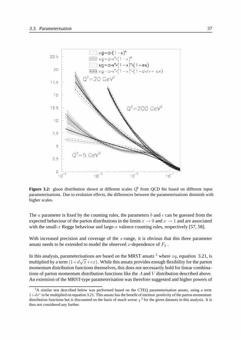
Figure 3.2: gluon distribution shown at different scales Q2 from QCD fits based on different inputparameterisations. Due to evolution effects, the differences between the parameterisations diminish withhigher scales.
The a parameter is fixed by the counting rules, the parameters b and c can be guessed from theexpected behaviour of the parton distributions in the limits x → 0 and x → 1 and are associatedwith the small-x Regge behaviour and large-x valence counting rules, respectively [57, 58].
With increased precision and coverage of the x-range, it is obvious that this three parameteransatz needs to be extended to model the observed x-dependence of F2 .
In this analysis, parameterisations are based on the MRST ansatz 2 where xq, equation 3.21, ismultiplied by a term (1+d
√x+ex). While this ansatz provides enough flexibility for the parton
momentum distribution functions themselves, this does not necessarily hold for linear combina-tions of parton momentum distribution functions like the A and V distribution described above.An extension of the MRST-type parameterisation was therefore suggested and higher powers of
2A similar test described below was performed based on the CTEQ parameterisation ansatz, using a term1+dxe to be multiplied on equation 3.21. This ansatz has the benefit of intrinsic positivity of the parton momentumdistribution functions but is discounted on the basis of much worse χ 2 for the given datasets in this analysis. It isthus not considered any further.
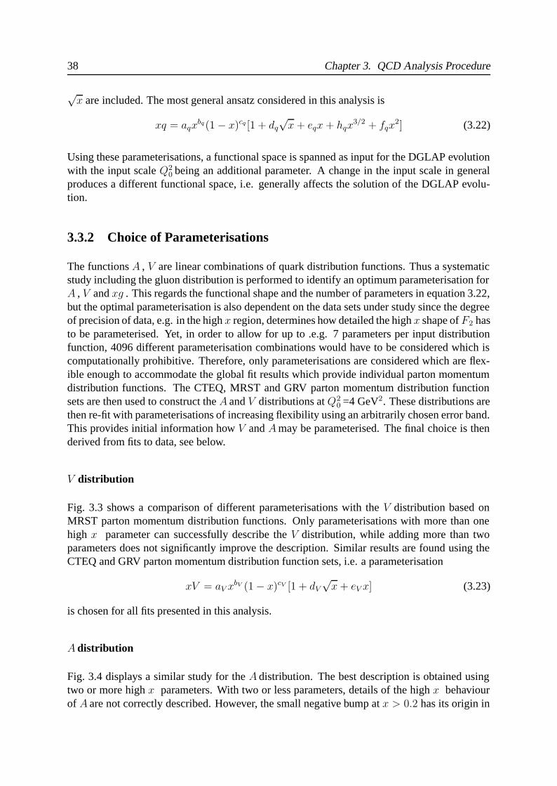
38 Chapter 3. QCD Analysis Procedure
√x are included. The most general ansatz considered in this analysis is
xq = aqxbq(1 − x)cq [1 + dq
√x + eqx + hqx
3/2 + fqx2] (3.22)
Using these parameterisations, a functional space is spanned as input for the DGLAP evolutionwith the input scale Q2
0 being an additional parameter. A change in the input scale in generalproduces a different functional space, i.e. generally affects the solution of the DGLAP evolu-tion.
3.3.2 Choice of Parameterisations
The functions A , V are linear combinations of quark distribution functions. Thus a systematicstudy including the gluon distribution is performed to identify an optimum parameterisation forA , V and xg . This regards the functional shape and the number of parameters in equation 3.22,but the optimal parameterisation is also dependent on the data sets under study since the degreeof precision of data, e.g. in the high x region, determines how detailed the high x shape of F2 hasto be parameterised. Yet, in order to allow for up to .e.g. 7 parameters per input distributionfunction, 4096 different parameterisation combinations would have to be considered which iscomputationally prohibitive. Therefore, only parameterisations are considered which are flex-ible enough to accommodate the global fit results which provide individual parton momentumdistribution functions. The CTEQ, MRST and GRV parton momentum distribution functionsets are then used to construct the A and V distributions at Q2
0 =4 GeV2. These distributions arethen re-fit with parameterisations of increasing flexibility using an arbitrarily chosen error band.This provides initial information how V and A may be parameterised. The final choice is thenderived from fits to data, see below.
V distribution
Fig. 3.3 shows a comparison of different parameterisations with the V distribution based onMRST parton momentum distribution functions. Only parameterisations with more than onehigh x parameter can successfully describe the V distribution, while adding more than twoparameters does not significantly improve the description. Similar results are found using theCTEQ and GRV parton momentum distribution function sets, i.e. a parameterisation
xV = aV xbV (1 − x)cV [1 + dV
√x + eV x] (3.23)
is chosen for all fits presented in this analysis.
A distribution
Fig. 3.4 displays a similar study for the A distribution. The best description is obtained usingtwo or more high x parameters. With two or less parameters, details of the high x behaviourof A are not correctly described. However, the small negative bump at x > 0.2 has its origin in
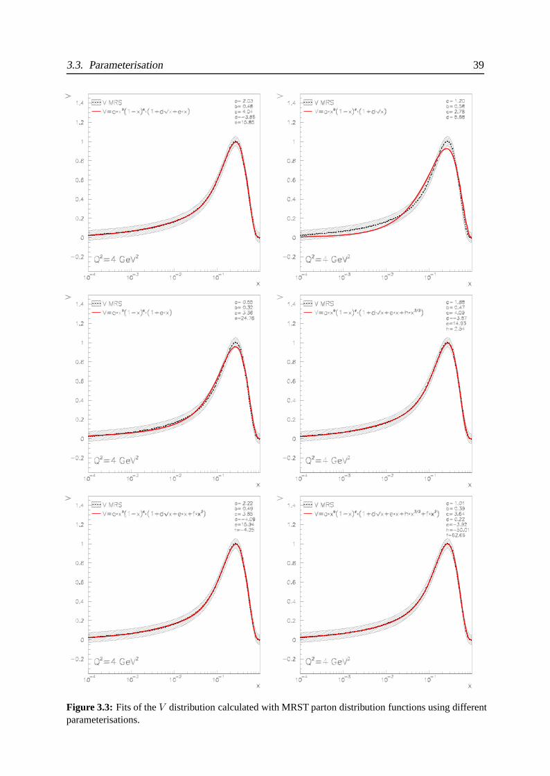
3.3. Parameterisation 39
Figure 3.3: Fits of the V distribution calculated with MRST parton distribution functions using differentparameterisations.
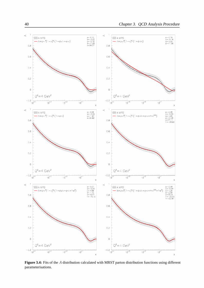
40 Chapter 3. QCD Analysis Procedure
Figure 3.4: Fits of the A distribution calculated with MRST parton distribution functions using differentparameterisations.
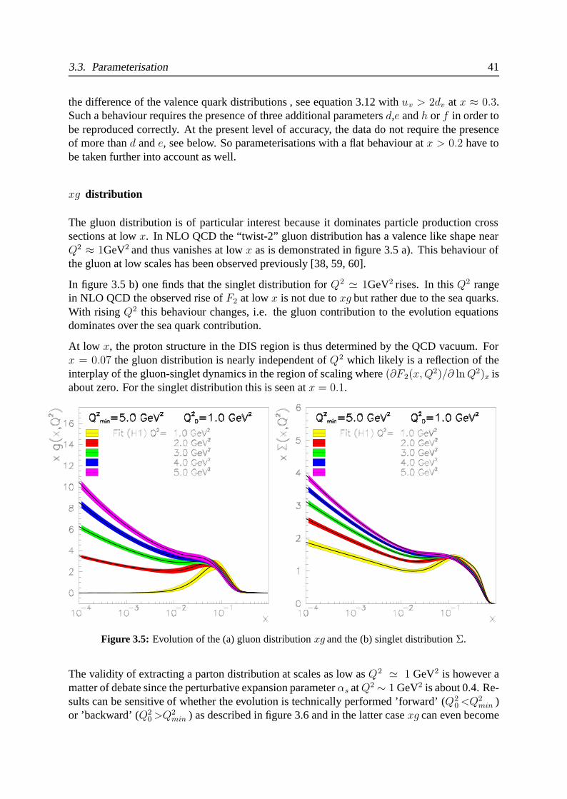
3.3. Parameterisation 41
the difference of the valence quark distributions , see equation 3.12 with uv > 2dv at x ≈ 0.3.Such a behaviour requires the presence of three additional parameters d,e and h or f in order tobe reproduced correctly. At the present level of accuracy, the data do not require the presenceof more than d and e, see below. So parameterisations with a flat behaviour at x > 0.2 have tobe taken further into account as well.
xg distribution
The gluon distribution is of particular interest because it dominates particle production crosssections at low x. In NLO QCD the “twist-2” gluon distribution has a valence like shape nearQ2 ≈ 1GeV2 and thus vanishes at low x as is demonstrated in figure 3.5 a). This behaviour ofthe gluon at low scales has been observed previously [38, 59, 60].
In figure 3.5 b) one finds that the singlet distribution for Q2 1GeV2 rises. In this Q2 rangein NLO QCD the observed rise of F2 at low x is not due to xg but rather due to the sea quarks.With rising Q2 this behaviour changes, i.e. the gluon contribution to the evolution equationsdominates over the sea quark contribution.
At low x, the proton structure in the DIS region is thus determined by the QCD vacuum. Forx = 0.07 the gluon distribution is nearly independent of Q2 which likely is a reflection of theinterplay of the gluon-singlet dynamics in the region of scaling where (∂F2(x, Q2)/∂ ln Q2)x isabout zero. For the singlet distribution this is seen at x = 0.1.
Figure 3.5: Evolution of the (a) gluon distribution xg and the (b) singlet distribution Σ.
The validity of extracting a parton distribution at scales as low as Q2 1 GeV2 is however amatter of debate since the perturbative expansion parameter αs at Q2 ∼ 1 GeV2 is about 0.4. Re-sults can be sensitive of whether the evolution is technically performed ’forward’ (Q2
0 <Q2min )
or ’backward’ (Q20 >Q2
min ) as described in figure 3.6 and in the latter case xg can even become
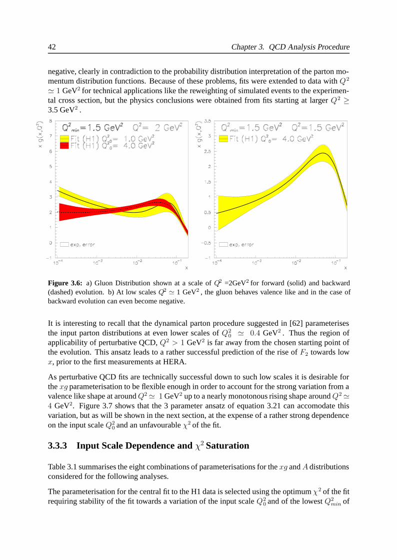
42 Chapter 3. QCD Analysis Procedure
negative, clearly in contradiction to the probability distribution interpretation of the parton mo-mentum distribution functions. Because of these problems, fits were extended to data with Q2
1 GeV2 for technical applications like the reweighting of simulated events to the experimen-tal cross section, but the physics conclusions were obtained from fits starting at larger Q2 ≥3.5 GeV2 .
Figure 3.6: a) Gluon Distribution shown at a scale of Q2 =2GeV2 for forward (solid) and backward(dashed) evolution. b) At low scales Q2 1 GeV2 , the gluon behaves valence like and in the case ofbackward evolution can even become negative.
It is interesting to recall that the dynamical parton procedure suggested in [62] parameterisesthe input parton distributions at even lower scales of Q2
0 0.4 GeV2 . Thus the region ofapplicability of perturbative QCD, Q2 > 1 GeV2 is far away from the chosen starting point ofthe evolution. This ansatz leads to a rather successful prediction of the rise of F2 towards lowx, prior to the first measurements at HERA.
As perturbative QCD fits are technically successful down to such low scales it is desirable forthe xg parameterisation to be flexible enough in order to account for the strong variation from avalence like shape at around Q2 1 GeV2 up to a nearly monotonous rising shape around Q2 4 GeV2. Figure 3.7 shows that the 3 parameter ansatz of equation 3.21 can accomodate thisvariation, but as will be shown in the next section, at the expense of a rather strong dependenceon the input scale Q2
0 and an unfavourable χ2 of the fit.
3.3.3 Input Scale Dependence and χ2 Saturation
Table 3.1 summarises the eight combinations of parameterisations for the xg and A distributionsconsidered for the following analyses.
The parameterisation for the central fit to the H1 data is selected using the optimum χ2 of the fitrequiring stability of the fit towards a variation of the input scale Q2
0 and of the lowest Q2min of
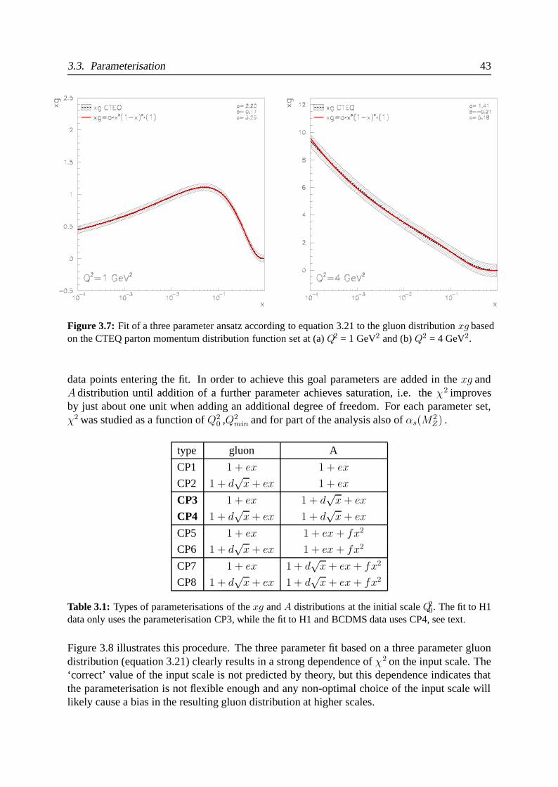
3.3. Parameterisation 43
Figure 3.7: Fit of a three parameter ansatz according to equation 3.21 to the gluon distribution xg basedon the CTEQ parton momentum distribution function set at (a) Q2 = 1 GeV2 and (b) Q2 = 4 GeV2.
data points entering the fit. In order to achieve this goal parameters are added in the xg andA distribution until addition of a further parameter achieves saturation, i.e. the χ2 improvesby just about one unit when adding an additional degree of freedom. For each parameter set,χ2 was studied as a function of Q2
0 ,Q2min and for part of the analysis also of αs(M
2Z) .
type gluon A
CP1 1 + ex 1 + ex
CP2 1 + d√
x + ex 1 + ex
CP3 1 + ex 1 + d√
x + ex
CP4 1 + d√
x + ex 1 + d√
x + ex
CP5 1 + ex 1 + ex + fx2
CP6 1 + d√
x + ex 1 + ex + fx2
CP7 1 + ex 1 + d√
x + ex + fx2
CP8 1 + d√
x + ex 1 + d√
x + ex + fx2
Table 3.1: Types of parameterisations of the xg and A distributions at the initial scale Q20. The fit to H1
data only uses the parameterisation CP3, while the fit to H1 and BCDMS data uses CP4, see text.
Figure 3.8 illustrates this procedure. The three parameter fit based on a three parameter gluondistribution (equation 3.21) clearly results in a strong dependence of χ2 on the input scale. The‘correct’ value of the input scale is not predicted by theory, but this dependence indicates thatthe parameterisation is not flexible enough and any non-optimal choice of the input scale willlikely cause a bias in the resulting gluon distribution at higher scales.
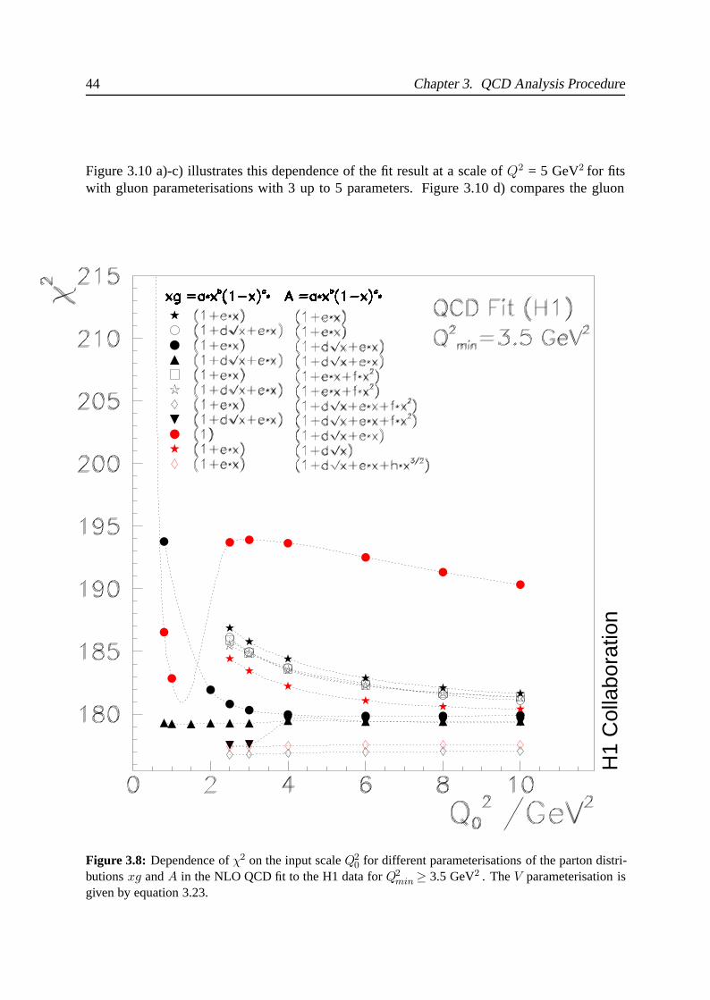
44 Chapter 3. QCD Analysis Procedure
Figure 3.10 a)-c) illustrates this dependence of the fit result at a scale of Q2 = 5 GeV2 for fitswith gluon parameterisations with 3 up to 5 parameters. Figure 3.10 d) compares the gluon
H1
Col
labo
ratio
n
Figure 3.8: Dependence of χ2 on the input scale Q20 for different parameterisations of the parton distri-
butions xg and A in the NLO QCD fit to the H1 data for Q2min ≥ 3.5 GeV2 . The V parameterisation is
given by equation 3.23.
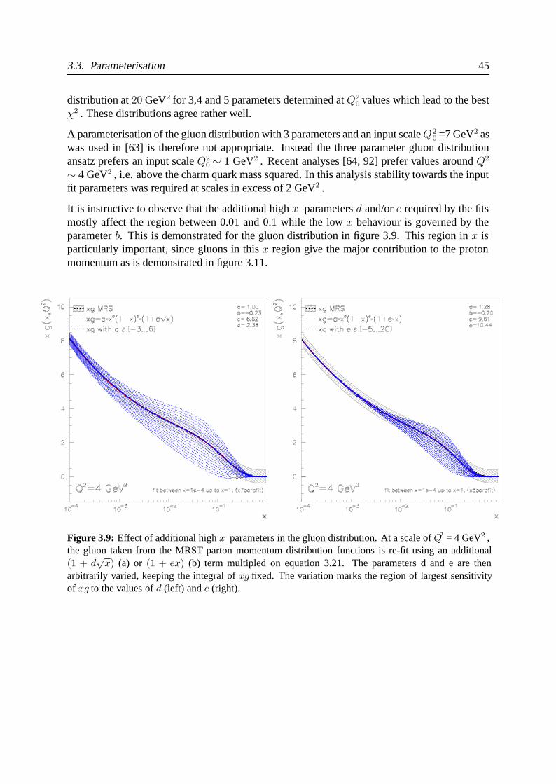
3.3. Parameterisation 45
distribution at 20 GeV2 for 3,4 and 5 parameters determined at Q20 values which lead to the best
χ2 . These distributions agree rather well.
A parameterisation of the gluon distribution with 3 parameters and an input scale Q20 =7 GeV2 as
was used in [63] is therefore not appropriate. Instead the three parameter gluon distributionansatz prefers an input scale Q2
0 ∼ 1 GeV2 . Recent analyses [64, 92] prefer values around Q2
∼ 4 GeV2 , i.e. above the charm quark mass squared. In this analysis stability towards the inputfit parameters was required at scales in excess of 2 GeV2 .
It is instructive to observe that the additional high x parameters d and/or e required by the fitsmostly affect the region between 0.01 and 0.1 while the low x behaviour is governed by theparameter b. This is demonstrated for the gluon distribution in figure 3.9. This region in x isparticularly important, since gluons in this x region give the major contribution to the protonmomentum as is demonstrated in figure 3.11.
Figure 3.9: Effect of additional high x parameters in the gluon distribution. At a scale of Q2 = 4 GeV2 ,the gluon taken from the MRST parton momentum distribution functions is re-fit using an additional(1 + d
√x) (a) or (1 + ex) (b) term multipled on equation 3.21. The parameters d and e are then
arbitrarily varied, keeping the integral of xg fixed. The variation marks the region of largest sensitivityof xg to the values of d (left) and e (right).
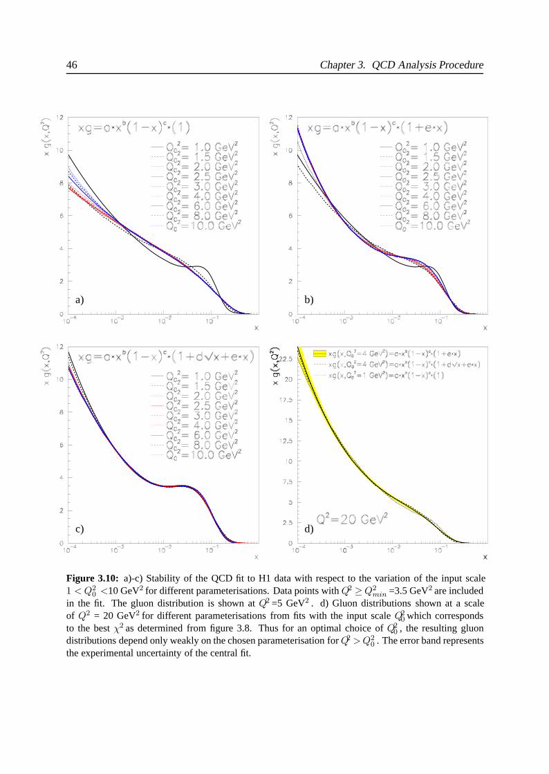
46 Chapter 3. QCD Analysis Procedure
a) b)
c) d)
Figure 3.10: a)-c) Stability of the QCD fit to H1 data with respect to the variation of the input scale1 < Q2
0 <10 GeV2 for different parameterisations. Data points with Q2 ≥ Q2min =3.5 GeV2 are included
in the fit. The gluon distribution is shown at Q2 =5 GeV2 . d) Gluon distributions shown at a scaleof Q2 = 20 GeV2 for different parameterisations from fits with the input scale Q2
0 which correspondsto the best χ2 as determined from figure 3.8. Thus for an optimal choice of Q2
0 , the resulting gluondistributions depend only weakly on the chosen parameterisation for Q2 > Q2
0 . The error band representsthe experimental uncertainty of the central fit.
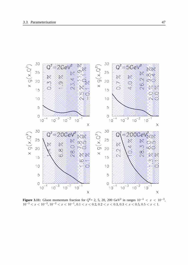
3.3. Parameterisation 47
Figure 3.11: Gluon momentum fraction for Q2= 2, 5, 20, 200 GeV2 in ranges 10−4 < x < 10−3,10−3 < x < 10−2, 10−2 < x < 10−1, 0.1 < x < 0.2, 0.2 < x < 0.3, 0.3 < x < 0.5, 0.5 < x < 1.
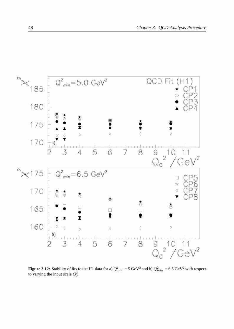
48 Chapter 3. QCD Analysis Procedure
a)
b)
Figure 3.12: Stability of fits to the H1 data for a) Q2min = 5 GeV2 and b) Q2
min = 6.5 GeV2 with respectto varying the input scale Q2
0 .
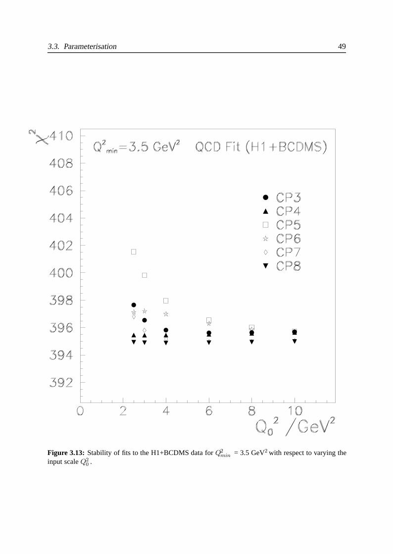
3.3. Parameterisation 49
Figure 3.13: Stability of fits to the H1+BCDMS data for Q2min = 3.5 GeV2 with respect to varying the
input scale Q20 .
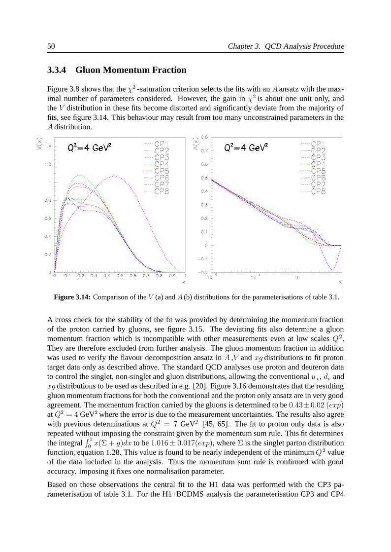
50 Chapter 3. QCD Analysis Procedure
3.3.4 Gluon Momentum Fraction
Figure 3.8 shows that the χ2 -saturation criterion selects the fits with an A ansatz with the max-imal number of parameters considered. However, the gain in χ2 is about one unit only, andthe V distribution in these fits become distorted and significantly deviate from the majority offits, see figure 3.14. This behaviour may result from too many unconstrained parameters in theA distribution.
Figure 3.14: Comparison of the V (a) and A (b) distributions for the parameterisations of table 3.1.
A cross check for the stability of the fit was provided by determining the momentum fractionof the proton carried by gluons, see figure 3.15. The deviating fits also determine a gluonmomentum fraction which is incompatible with other measurements even at low scales Q2.They are therefore excluded from further analysis. The gluon momentum fraction in additionwas used to verify the flavour decomposition ansatz in A ,V and xg distributions to fit protontarget data only as described above. The standard QCD analyses use proton and deuteron datato control the singlet, non-singlet and gluon distributions, allowing the conventional u v, dv andxg distributions to be used as described in e.g. [20]. Figure 3.16 demonstrates that the resultinggluon momentum fractions for both the conventional and the proton only ansatz are in very goodagreement. The momentum fraction carried by the gluons is determined to be 0.43±0.02 (exp)at Q2 = 4 GeV2 where the error is due to the measurement uncertainties. The results also agreewith previous determinations at Q2 = 7 GeV2 [45, 65]. The fit to proton only data is alsorepeated without imposing the constraint given by the momentum sum rule. This fit determinesthe integral
∫ 1
0x(Σ + g)dx to be 1.016± 0.017(exp), where Σ is the singlet parton distribution
function, equation 1.28. This value is found to be nearly independent of the minimum Q2 valueof the data included in the analysis. Thus the momentum sum rule is confirmed with goodaccuracy. Imposing it fixes one normalisation parameter.
Based on these observations the central fit to the H1 data was performed with the CP3 pa-rameterisation of table 3.1. For the H1+BCDMS analysis the parameterisation CP3 and CP4

3.3. Parameterisation 51
were found to be adequate by the same procedure for the central fit of Q2min =3.5 GeV2 . Since,
however, parameterisation CP3 proved slightly more vulnerable to variations of Q2min than CP4,
parameterisation CP4 was selected for the central H1+BCDMS fit. This allowed for more flex-ibility at high x as required by the more accurate high x data in the fit.
In all subsequent studies however were also performed with the alternative ansatz CP1-CP2,and CP4-5 and CP8 which yielded the correct momentum fraction to cross check the results.As is demonstrated in figure 3.12, the parameterisation ansatz CP3 also proved adequate undervariation of Q2
min .
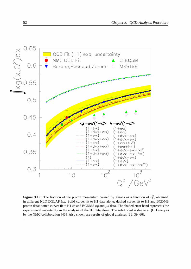
52 Chapter 3. QCD Analysis Procedure∫
Figure 3.15: The fraction of the proton momentum carried by gluons as a function of Q2, obtainedin different NLO DGLAP fits. Solid curve: fit to H1 data alone; dashed curve: fit to H1 and BCDMSproton data; dotted curve: fit to H1 ep and BCDMS μp and μd data. The shaded error band represents theexperimental uncertainty in the analysis of the H1 data alone. The solid point is due to a QCD analysisby the NMC collaboration [45]. Also shown are results of global analyses [38, 39, 66]..
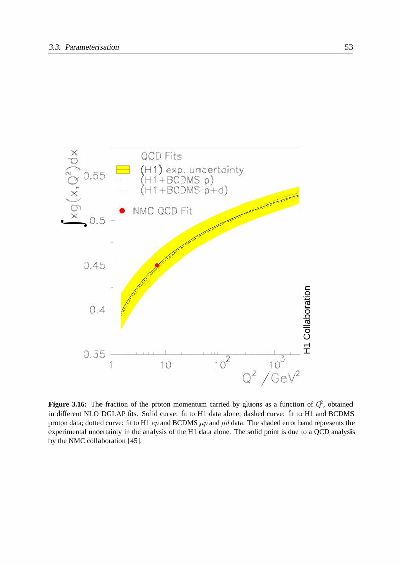
3.3. Parameterisation 53
H1
Col
labo
ratio
n
∫
Figure 3.16: The fraction of the proton momentum carried by gluons as a function of Q2, obtainedin different NLO DGLAP fits. Solid curve: fit to H1 data alone; dashed curve: fit to H1 and BCDMSproton data; dotted curve: fit to H1 ep and BCDMS μp and μd data. The shaded error band represents theexperimental uncertainty in the analysis of the H1 data alone. The solid point is due to a QCD analysisby the NMC collaboration [45].
54 Chapter 3. QCD Analysis Procedure
3.4 Definition of Minimization Procedure
3.4.1 Definition of χ2
The fit parameters are determined by finding the least square deviations between the theoreti-cal prediction of the reduced cross section σr
th and the measured reduced cross section σrexp
minimizing
χ2 ∑
i
[σexpr (xi, Q
2i ) − σth
r (xi, Q2i )]
2
δ2i,unc + δ2
i,stat
. (3.24)
The sum over i runs over all data points of all datasets involved. The theoretical neutral cur-rent double differential cross section is computed in its reduced form using equation 1.7. Thestructure functions F2 and FL are calculated using equations 1.20 and 1.22, respectively.
3.4.2 Correlated Systematic Error Treatment
The experimental systematic errors introduce point-to-point correlations which are not properlytaken into account by equation 3.24. Treatment of these correlations is provided following amethod proposed by [66].
In principle, the evaluation of correlated systematic errors and their propagation (see below) canbe incorporated in a standard Hessian matrix approach, see [67, 42]. However, the many moreparameters in the fit in practice require the inversion of matrices of large dimensions whichis numerically unstable if the eigenvalues of the Hessian matrix span a large range of values.Therefore, in this analysis a different method is used by which the correlated uncertainties areparameterized by a set of fit parameters sλ where λ indicates the systematic error source asdescribed in table 2.1. It has been shown [43] that this method is equivalent to the standardHessian matrix approach.
Therefore, the model prediction σthr,i(p) corresponding to a set of model fit parameters p and
systematics parameters sλ at a given point (xi, Q2i ) is modified according to
σthr,i(p) → σth
r,i(p, s) = σthr,i(p) × (1 +
∑λ
sλδsystiλ ) (3.25)
where δsystiλ is the relative systematic error of data point i due to source λ. For the further statis-
tically correct treatment of the correlated systematic errors and their propagation it is assumedthat the sλ are uncorrelated and gaussian distributed with zero mean and unit variance3. A valueof sλ = ±1 therefore indicates a deviation of the measurement of one standard deviation awayfrom the central value.
3This also implies averaging the effect of asymmetric error sources. Note that these assumption can be violatedwith certain error sources, i.e. noise treatment.
3.4. Definition of Minimization Procedure 55
Further systematic error sources are the relative normalizations of the data sets which are mainlydetermined by the luminosity measurements and global trigger and reconstruction efficiencies.Accordingly, further correlated systematic parameters νk are introduced which estimate thenumber of standard deviations of the normalization uncertainty δnorm
k of experimental data setk.
For the parameters sλ and νk related to systematics counter (penalty) terms are introduced intothe χ2 definition to control their variation in ±1σ limits. The full χ2 definition therefore readsfor a fit to nexp datasets with relative normalization uncertainties δnorm
k , np(k) data points andns(k) correlated systematic error sources sλ which give rise to a relative correlated systematicerror δsyst
iλ on the cross section, as
χ2 =
nexp∑k
np(k)∑i
[σr,iexp − σr,i
th × (1 − νkδnormk − ∑ns(k)
λ sλ,kδsystiλ )]
δ2i,sta + δ2
i,unc
+∑
k
ν2k +
∑k
∑λ
(sexpλ )2. (3.26)
Note that the systematics parameters sλ are not counted as free parameters since they are con-strained by the penalty terms in the χ2 definition. The QCD fit program used determines thefree parameters using the MINUIT minimization program [68] and the systematics are fitted ineach MINUIT iteration using a least square minimization procedure exploiting the linear depen-dence of the χ2 on the systematics parameters sλ, saving computer time [69]. Furthermore, thederivatives of the χ2 with respect to the systematics parameters are determined which is neededfor the error propagation.
3.4.3 Error Propagation
In order to propagate the statistical and systematic uncertainties of the cross section on theparton momentum distribution functions, two Hessian matrices M and C are computed at theminimum χ2
min
Mλμ =1
2
∂2χ2
∂pλ∂pμ, Cλμ =
1
2
∂2χ2
∂pλ∂sμ, (3.27)
The statistical and systematic covariance matrices are then given by [66]
Vstat = M−1, Vsyst = M−1CCTM−1, (3.28)
For any function G which depends on the model parameters p, G = G(p). The error ΔG is thenobtained using
ΔG2 =∑
λ
∑μ
∂G
∂pλ
Vλμ∂G
∂pμ
(3.29)
where the matrix Vλν corresponds to Vstat, Vsyst or both added in quadrature for the statistical,systematic and the total error.
56 Chapter 3. QCD Analysis Procedure
In order to define envelopes for a function G(p) which is minimal for a set of model parameterspf , the variation of these parameters p − pf can be found by
(p − pf )λ = ±∑
μ Vλμ∂Gpµ√
ΔG2(3.30)
These envelopes are the error bands shown in all subsequent figures. They are defining the 68%probability for a given point G(p) (which can be thought of e.g. the gluon distribution at a fixedx and Q2) to stay in the envelope under variation around the minimum of a fit parameter p byits uncertainty.
Note that this statistical interpretation relies on simplifying assumptions which in practice areoften not precisely met, e.g. gaussian fluctuating systematic errors. Furthermore, especially athigh x, the estimation can be biased by the parameterisation as well.
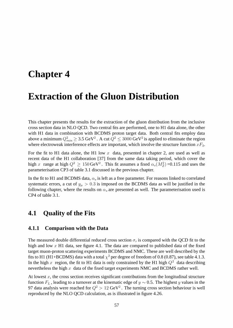
Chapter 4
Extraction of the Gluon Distribution
This chapter presents the results for the extraction of the gluon distribution from the inclusivecross section data in NLO QCD. Two central fits are performed, one to H1 data alone, the otherwith H1 data in combination with BCDMS proton target data. Both central fits employ dataabove a minimum Q2
min ≥ 3.5 GeV2 . A cut Q2 ≤ 3000 GeV2 is applied to eliminate the regionwhere electroweak interference effects are important, which involve the structure function xF3.
For the fit to H1 data alone, the H1 low x data, presented in chapter 2, are used as well asrecent data of the H1 collaboration [37] from the same data taking period, which cover thehigh x range at high Q2 ≥ 150 GeV2 . This fit assumes a fixed αs(M
2Z) =0.115 and uses the
parameterisation CP3 of table 3.1 discussed in the previous chapter.
In the fit to H1 and BCDMS data, αs is left as a free parameter. For reasons linked to correlatedsystematic errors, a cut of yμ > 0.3 is imposed on the BCDMS data as will be justified in thefollowing chapter, where the results on αs are presented as well. The parameterisation used isCP4 of table 3.1.
4.1 Quality of the Fits
4.1.1 Comparison with the Data
The measured double differential reduced cross section σr is compared with the QCD fit to thehigh and low x H1 data, see figure 4.1. The data are compared to published data of the fixedtarget muon-proton scattering experiments BCDMS and NMC. These are well described by thefits to H1 (H1+BCDMS) data with a total χ2 per degree of freedom of 0.8 (0.87), see table 4.1.3.In the high x region, the fit to H1 data is only constrained by the H1 high Q2 data describingnevertheless the high x data of the fixed target experiments NMC and BCDMS rather well.
At lowest x, the cross section receives significant contributions from the longitudinal structurefunction FL , leading to a turnover at the kinematic edge of y ∼ 0.5. The highest y values in the97 data analysis were reached for Q2 > 12 GeV2 . The turning cross section behaviour is wellreproduced by the NLO QCD calculation, as is illustrated in figure 4.26.
57
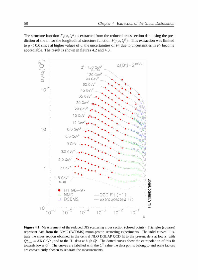
58 Chapter 4. Extraction of the Gluon Distribution
The structure function F2(x, Q2) is extracted from the reduced cross section data using the pre-diction of the fit for the longitudinal structure function FL(x, Q2) . This extraction was limitedto y < 0.6 since at higher values of y, the uncertainties of F2 due to uncertainties in FL becomeappreciable. The result is shown in figures 4.2 and 4.3.
H1
Col
labo
ratio
n
Figure 4.1: Measurement of the reduced DIS scattering cross section (closed points). Triangles (squares)represent data from the NMC (BCDMS) muon-proton scattering experiments. The solid curves illus-trate the cross section obtained in the central NLO DGLAP QCD fit to the present data at low x, withQ2
min = 3.5 GeV2 , and to the H1 data at high Q2. The dotted curves show the extrapolation of this fittowards lower Q2. The curves are labelled with the Q2 value the data points belong to and scale factorsare conveniently chosen to separate the measurements.
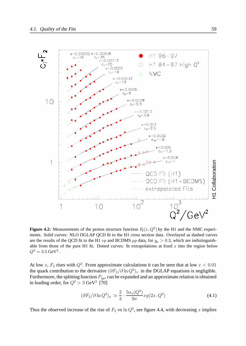
4.1. Quality of the Fits 59
H1
Col
labo
ratio
n
Figure 4.2: Measurements of the proton structure function F2(x,Q2) by the H1 and the NMC experi-ments. Solid curves: NLO DGLAP QCD fit to the H1 cross section data. Overlayed as dashed curvesare the results of the QCD fit to the H1 ep and BCDMS μp data, for yμ > 0.3, which are indistinguish-able from those of the pure H1 fit. Dotted curves: fit extrapolations at fixed x into the region belowQ2 = 3.5 GeV2 .
At low x, F2 rises with Q2. From approximate calculations it can be seen that at low x < 0.01the quark contribution to the derivative (∂F2/∂ lnQ2)x in the DGLAP equations is negligible.Furthermore, the splitting function Pqg, can be expanded and an approximate relation is obtainedin leading order, for Q2 > 3 GeV2 [70]
(∂F2/∂ ln Q2)x 2
3· 5αs(Q
2)
9πxg(2x, Q2) (4.1)
Thus the observed increase of the rise of F2 vs ln Q2, see figure 4.4, with decreasing x implies
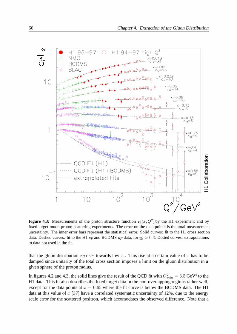
60 Chapter 4. Extraction of the Gluon Distribution
H1
Col
labo
ratio
n
Figure 4.3: Measurements of the proton structure function F2(x,Q2) by the H1 experiment and byfixed target muon-proton scattering experiments. The error on the data points is the total measurementuncertainty. The inner error bars represent the statistical error. Solid curves: fit to the H1 cross sectiondata. Dashed curves: fit to the H1 ep and BCDMS μp data, for yμ > 0.3. Dotted curves: extrapolationsto data not used in the fit.
that the gluon distribution xg rises towards low x . This rise at a certain value of x has to bedamped since unitarity of the total cross section imposes a limit on the gluon distribution in agiven sphere of the proton radius.
In figures 4.2 and 4.3, the solid lines give the result of the QCD fit with Q2min = 3.5 GeV2 to the
H1 data. This fit also describes the fixed target data in the non-overlapping regions rather well,except for the data points at x = 0.65 where the fit curve is below the BCDMS data. The H1data at this value of x [37] have a correlated systematic uncertainty of 12%, due to the energyscale error for the scattered positron, which accomodates the observed difference. Note that a
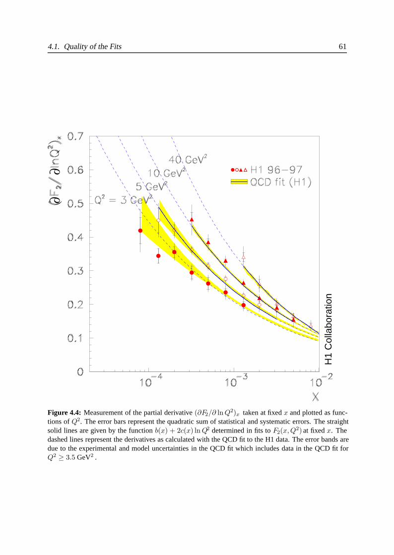
4.1. Quality of the Fits 61∂
∂
H1
Col
labo
ratio
n
Figure 4.4: Measurement of the partial derivative (∂F2/∂ ln Q2)x taken at fixed x and plotted as func-tions of Q2. The error bars represent the quadratic sum of statistical and systematic errors. The straightsolid lines are given by the function b(x) + 2c(x) ln Q2 determined in fits to F2(x,Q2) at fixed x. Thedashed lines represent the derivatives as calculated with the QCD fit to the H1 data. The error bands aredue to the experimental and model uncertainties in the QCD fit which includes data in the QCD fit forQ2 ≥ 3.5 GeV2 .

62 Chapter 4. Extraction of the Gluon Distribution
new, preliminary H1 measurement [71] of F2(x, Q2) at high Q2 and x results in a consistentbut larger F2 values for x = 0.65 which may resolve the difference between the BCDMS andH1 high x data observed here.
4.1.2 Pull Distributions
Table 4.1.3 summarises the fit results for the H1 and H1+BCDMS fits. The χ2 per degree offreedom is slightly below 1 indicating an overestimation of the uncorrelated errors. Figure 4.5shows the pull distribution for the individual datasets in the fit to H1 data alone, 4.6 in the fit toH1 and BCDMS data. The pulls are defined as
pull =Data − csys ∗ Theory
uncorr.error
where csys reflects the effect of the correlated error sources.
4.1.3 QCD Model Parameters
Table 4.2 presents the extracted QCD parameters of the fits to the H1 data alone in the fullkinematic range and for y < 0.35 (see below) and to the H1 and BCDMS data. The resultfor the parameter cg comes out to be rather large as compared to the dimensional counting ruleexpectation [72]. A fit with dg = eg = 0 to H1 and BCDMS data, however, yields cg = 6.5 forthe fit to H1 and BCDMS data, not far from dimensional counting rule expectations [72], yetwith a deteriorated χ2. Note that the gluon normalisation ag and the low x parameter bg areobserved to be strongly correlated, explaining the different values obtained from the analysisof H1 data without and with a cut in y. The resulting gluon distributions, however, agree verywell, see below.
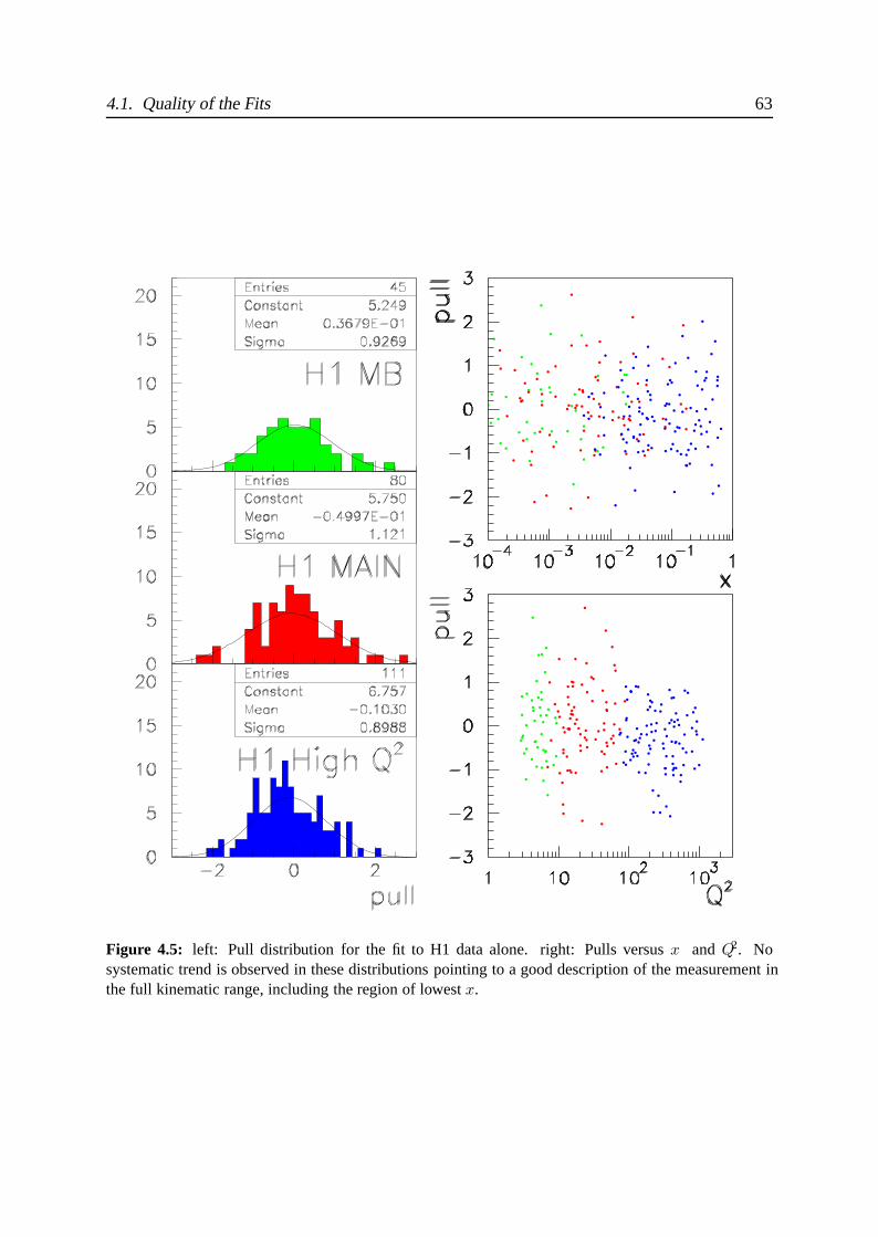
4.1. Quality of the Fits 63
Figure 4.5: left: Pull distribution for the fit to H1 data alone. right: Pulls versus x and Q2. Nosystematic trend is observed in these distributions pointing to a good description of the measurement inthe full kinematic range, including the region of lowest x.
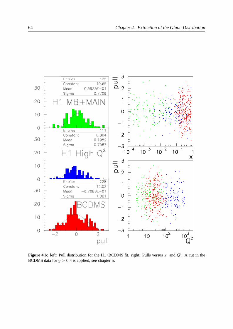
64 Chapter 4. Extraction of the Gluon Distribution
Figure 4.6: left: Pull distribution for the H1+BCDMS fit. right: Pulls versus x and Q2. A cut in theBCDMS data for y > 0.3 is applied, see chapter 5.
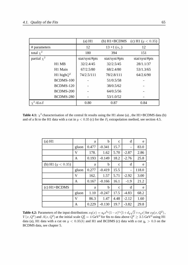
4.1. Quality of the Fits 65
(a) H1 (b) H1+BCDMS (c) H1 (y < 0.35)
# parameters 12 13 +1 (αs ) 12
total χ2 180 394 151
partial χ2 stat/syst/#pts stat/syst/#pts stat/syst/#pts
H1 MB 32/2.4/45 32/2.5/45 28/1.1/37
H1 Main 67/2.5/80 68/2.4/80 53/1.3/65
H1 highQ2 74/2.5/111 78/2.8/111 64/2.6/90
BCDMS-100 - 51/0.5/58 -
BCDMS-120 - 38/0.5/62 -
BCDMS-200 - 64/0.5/56 -
BCDMS-280 - 53/1.0/52 -
χ2 /d.o.f 0.80 0.87 0.84
Table 4.1: χ2 characterisation of the central fit results using the H1 alone (a) , the H1+BCDMS data (b)and of a fit to the H1 data with a cut in y < 0.35 (c) for the FL extrapolation method, see section 4.5.
(a) H1 a b c d e
gluon 0.477 -0.341 15.7 - 83.0
V 178. 1.62 5.70 -2.87 2.86
A 0.193 -0.149 18.2 -2.76 25.8
(b) H1 (y < 0.35) a b c d e
gluon 0.277 -0.419 15.5 - 118.0
V 162. 1.57 5.71 -2.92 3.00
A 0.167 -0.166 16.1 -1.9 21.2
(c) H1+BCDMS a b c d e
gluon 1.10 -0.247 17.5 -4.83 68.2
V 86.3 1.47 4.48 -2.12 1.60
A 0.229 -0.130 19.7 -3.82 29.8
Table 4.2: Parameters of the input distributions xq(x) = aqxbq(1−x)cq [1+dq
√x+eqx] for xg(x,Q2) ,
V (x,Q2) and A(x,Q2) at the initial scale Q20 = 4 GeV2 for fits to data above Q2 ≥ 3.5 GeV2 using H1
data (a), H1 data with a cut on y < 0.35(b) and H1 and BCDMS (c) data with a cut yμ > 0.3 on theBCDMS data, see chapter 5.
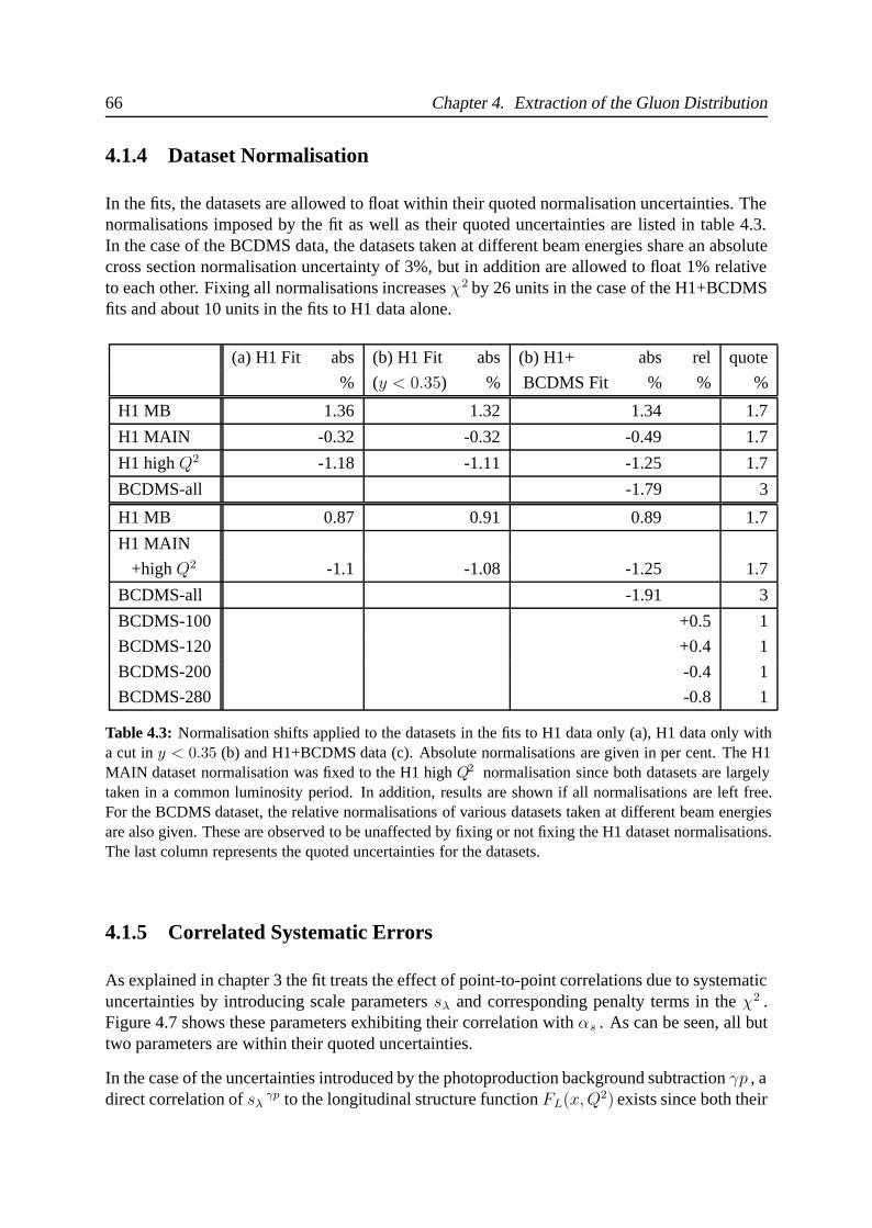
66 Chapter 4. Extraction of the Gluon Distribution
4.1.4 Dataset Normalisation
In the fits, the datasets are allowed to float within their quoted normalisation uncertainties. Thenormalisations imposed by the fit as well as their quoted uncertainties are listed in table 4.3.In the case of the BCDMS data, the datasets taken at different beam energies share an absolutecross section normalisation uncertainty of 3%, but in addition are allowed to float 1% relativeto each other. Fixing all normalisations increases χ2 by 26 units in the case of the H1+BCDMSfits and about 10 units in the fits to H1 data alone.
(a) H1 Fit abs (b) H1 Fit abs (b) H1+ abs rel quote
% (y < 0.35) % BCDMS Fit % % %
H1 MB 1.36 1.32 1.34 1.7
H1 MAIN -0.32 -0.32 -0.49 1.7
H1 high Q2 -1.18 -1.11 -1.25 1.7
BCDMS-all -1.79 3
H1 MB 0.87 0.91 0.89 1.7
H1 MAIN
+high Q2 -1.1 -1.08 -1.25 1.7
BCDMS-all -1.91 3
BCDMS-100 +0.5 1
BCDMS-120 +0.4 1
BCDMS-200 -0.4 1
BCDMS-280 -0.8 1
Table 4.3: Normalisation shifts applied to the datasets in the fits to H1 data only (a), H1 data only witha cut in y < 0.35 (b) and H1+BCDMS data (c). Absolute normalisations are given in per cent. The H1MAIN dataset normalisation was fixed to the H1 high Q2 normalisation since both datasets are largelytaken in a common luminosity period. In addition, results are shown if all normalisations are left free.For the BCDMS dataset, the relative normalisations of various datasets taken at different beam energiesare also given. These are observed to be unaffected by fixing or not fixing the H1 dataset normalisations.The last column represents the quoted uncertainties for the datasets.
4.1.5 Correlated Systematic Errors
As explained in chapter 3 the fit treats the effect of point-to-point correlations due to systematicuncertainties by introducing scale parameters sλ and corresponding penalty terms in the χ2 .Figure 4.7 shows these parameters exhibiting their correlation with αs . As can be seen, all buttwo parameters are within their quoted uncertainties.
In the case of the uncertainties introduced by the photoproduction background subtraction γp , adirect correlation of sλ
γp to the longitudinal structure function FL(x, Q2) exists since both their
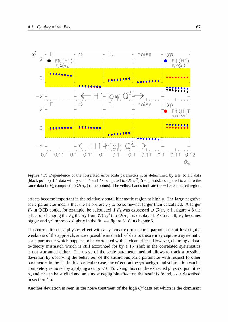
4.1. Quality of the Fits 67
Figure 4.7: Dependence of the correlated error scale parameters sλ as determined by a fit to H1 data(black points), H1 data with y < 0.35 and FL computed to O(αs
2) (red points), compared to a fit to thesame data fit FL computed to O(αs ) (blue points). The yellow bands indicate the ±1 σ estimated region.
effects become important in the relatively small kinematic region at high y. The large negativescale parameter means that the fit prefers FL to be somewhat larger than calculated. A largerFL in QCD could, for example, be calculated if FL was expressed to O(αs ): in figure 4.8 theeffect of changing the FL theory from O(αs
2) to O(αs ) is displayed. As a result, FL becomesbigger and χ2 improves slightly in the fit, see figure 5.18 in chapter 5.
This correlation of a physics effect with a systematic error source parameter is at first sight aweakness of the approach, since a possible mismatch of data to theory may capture a systematicscale parameter which happens to be correlated with such an effect. However, claiming a data-to-theory mismatch which is still accounted for by a 1σ shift in the correlated systematicsis not warranted either. The usage of the scale parameter method allows to track a possibledeviation by observing the behaviour of the suspicious scale parameter with respect to otherparameters in the fit. In this particular case, the effect on the γp background subtraction can becompletely removed by applying a cut y < 0.35. Using this cut, the extracted physics quantitiesαs and xg can be studied and an almost negligible effect on the result is found, as is describedin section 4.5.
Another deviation is seen in the noise treatment of the high Q2 data set which is the dominant
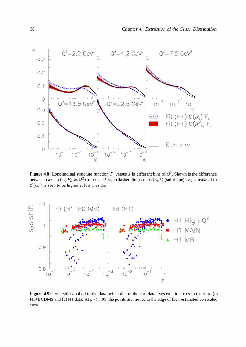
68 Chapter 4. Extraction of the Gluon Distribution
Figure 4.8: Longitudinal structure function FL versus x in different bins of Q2. Shown is the differencebetween calculating FL(x,Q2) to order O(αs ) (dashed line) and O(αs
2) (solid line). FL calculated toO(αs ) is seen to be higher at low x as the
Figure 4.9: Total shift applied to the data points due to the correlated systematic errors in the fit to (a)H1+BCDMS and (b) H1 data. At y < 0.05, the points are moved to the edge of their estimated correlatederror.
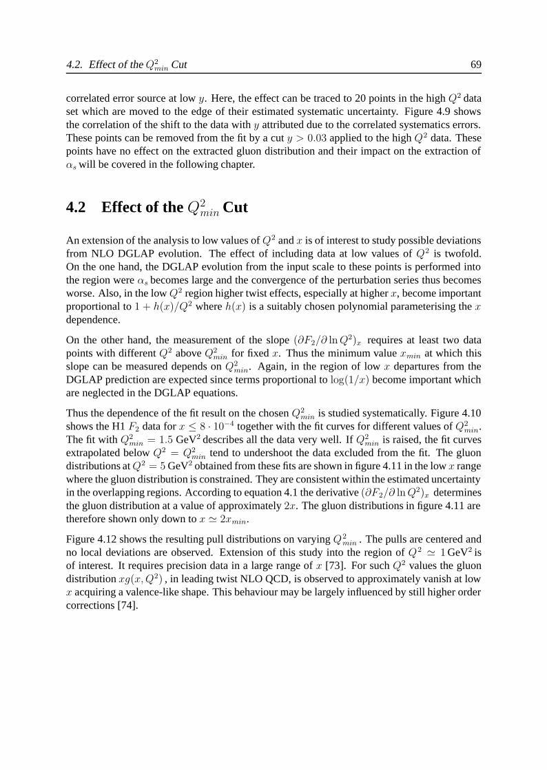
4.2. Effect of the Q2min Cut 69
correlated error source at low y. Here, the effect can be traced to 20 points in the high Q2 dataset which are moved to the edge of their estimated systematic uncertainty. Figure 4.9 showsthe correlation of the shift to the data with y attributed due to the correlated systematics errors.These points can be removed from the fit by a cut y > 0.03 applied to the high Q2 data. Thesepoints have no effect on the extracted gluon distribution and their impact on the extraction ofαs will be covered in the following chapter.
4.2 Effect of the Q2min Cut
An extension of the analysis to low values of Q2 and x is of interest to study possible deviationsfrom NLO DGLAP evolution. The effect of including data at low values of Q2 is twofold.On the one hand, the DGLAP evolution from the input scale to these points is performed intothe region were αs becomes large and the convergence of the perturbation series thus becomesworse. Also, in the low Q2 region higher twist effects, especially at higher x, become importantproportional to 1 + h(x)/Q2 where h(x) is a suitably chosen polynomial parameterising the xdependence.
On the other hand, the measurement of the slope (∂F2/∂ ln Q2)x requires at least two datapoints with different Q2 above Q2
min for fixed x. Thus the minimum value xmin at which thisslope can be measured depends on Q2
min. Again, in the region of low x departures from theDGLAP prediction are expected since terms proportional to log(1/x) become important whichare neglected in the DGLAP equations.
Thus the dependence of the fit result on the chosen Q2min is studied systematically. Figure 4.10
shows the H1 F2 data for x ≤ 8 · 10−4 together with the fit curves for different values of Q2min.
The fit with Q2min = 1.5 GeV2 describes all the data very well. If Q2
min is raised, the fit curvesextrapolated below Q2 = Q2
min tend to undershoot the data excluded from the fit. The gluondistributions at Q2 = 5 GeV2 obtained from these fits are shown in figure 4.11 in the low x rangewhere the gluon distribution is constrained. They are consistent within the estimated uncertaintyin the overlapping regions. According to equation 4.1 the derivative (∂F2/∂ ln Q2)x determinesthe gluon distribution at a value of approximately 2x. The gluon distributions in figure 4.11 aretherefore shown only down to x 2xmin.
Figure 4.12 shows the resulting pull distributions on varying Q2min . The pulls are centered and
no local deviations are observed. Extension of this study into the region of Q2 1 GeV2 isof interest. It requires precision data in a large range of x [73]. For such Q2 values the gluondistribution xg(x, Q2) , in leading twist NLO QCD, is observed to approximately vanish at lowx acquiring a valence-like shape. This behaviour may be largely influenced by still higher ordercorrections [74].
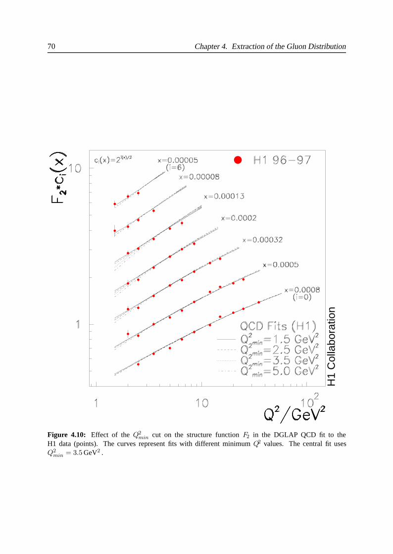
70 Chapter 4. Extraction of the Gluon Distribution
H1
Col
labo
ratio
n
Figure 4.10: Effect of the Q2min cut on the structure function F2 in the DGLAP QCD fit to the
H1 data (points). The curves represent fits with different minimum Q2 values. The central fit usesQ2
min = 3.5 GeV2 .
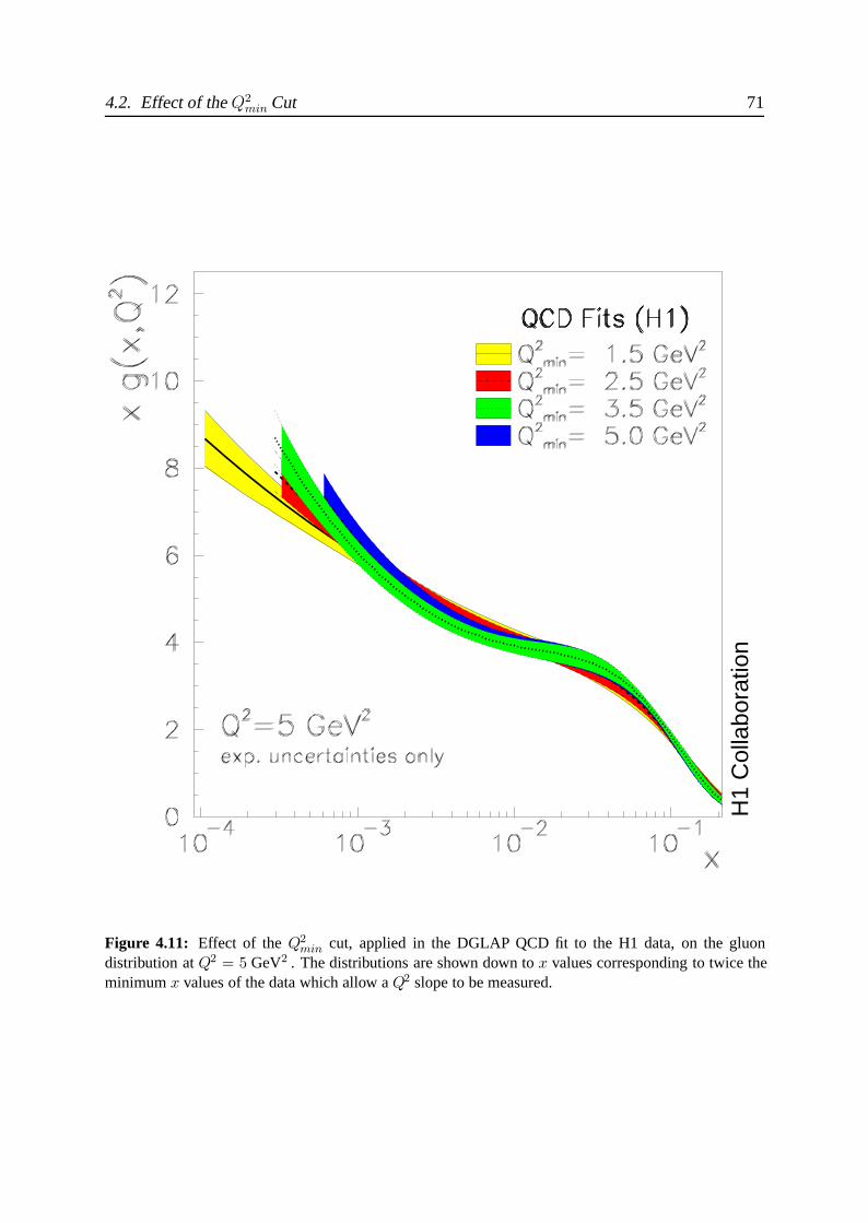
4.2. Effect of the Q2min Cut 71
H1
Col
labo
ratio
n
Figure 4.11: Effect of the Q2min cut, applied in the DGLAP QCD fit to the H1 data, on the gluon
distribution at Q2 = 5 GeV2 . The distributions are shown down to x values corresponding to twice theminimum x values of the data which allow a Q2 slope to be measured.
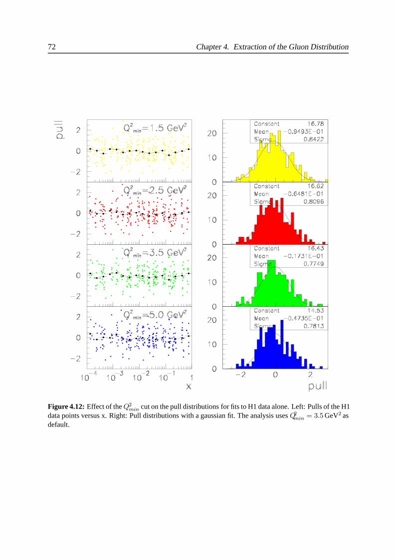
72 Chapter 4. Extraction of the Gluon Distribution
Figure 4.12: Effect of the Q2min cut on the pull distributions for fits to H1 data alone. Left: Pulls of the H1
data points versus x. Right: Pull distributions with a gaussian fit. The analysis uses Q2min = 3.5 GeV2 as
default.
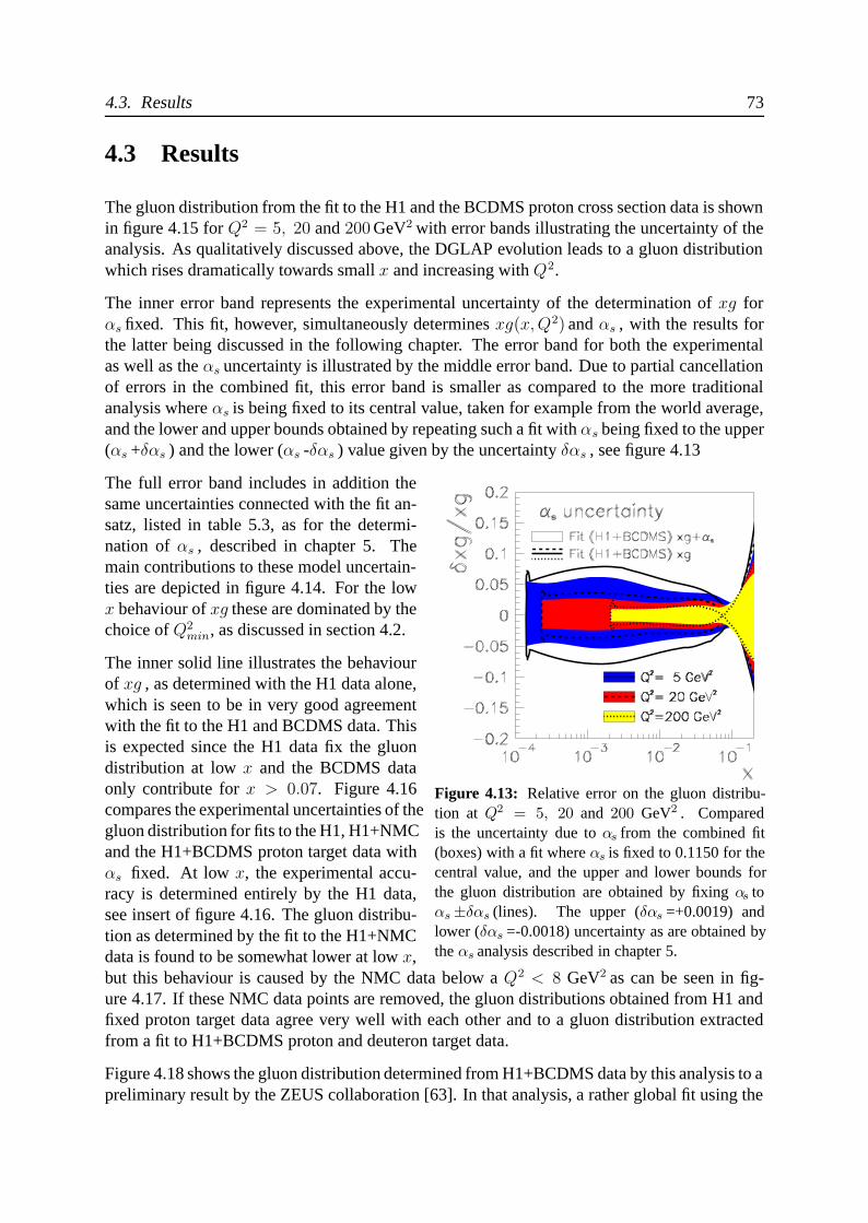
4.3. Results 73
4.3 Results
The gluon distribution from the fit to the H1 and the BCDMS proton cross section data is shownin figure 4.15 for Q2 = 5, 20 and 200 GeV2 with error bands illustrating the uncertainty of theanalysis. As qualitatively discussed above, the DGLAP evolution leads to a gluon distributionwhich rises dramatically towards small x and increasing with Q2.
The inner error band represents the experimental uncertainty of the determination of xg forαs fixed. This fit, however, simultaneously determines xg(x, Q2) and αs , with the results forthe latter being discussed in the following chapter. The error band for both the experimentalas well as the αs uncertainty is illustrated by the middle error band. Due to partial cancellationof errors in the combined fit, this error band is smaller as compared to the more traditionalanalysis where αs is being fixed to its central value, taken for example from the world average,and the lower and upper bounds obtained by repeating such a fit with αs being fixed to the upper(αs +δαs ) and the lower (αs -δαs ) value given by the uncertainty δαs , see figure 4.13
The full error band includes in addition the
Figure 4.13: Relative error on the gluon distribu-tion at Q2 = 5, 20 and 200 GeV2 . Comparedis the uncertainty due to αs from the combined fit(boxes) with a fit where αs is fixed to 0.1150 for thecentral value, and the upper and lower bounds forthe gluon distribution are obtained by fixing αs toαs ±δαs (lines). The upper (δαs =+0.0019) andlower (δαs =-0.0018) uncertainty as are obtained bythe αs analysis described in chapter 5.
same uncertainties connected with the fit an-satz, listed in table 5.3, as for the determi-nation of αs , described in chapter 5. Themain contributions to these model uncertain-ties are depicted in figure 4.14. For the lowx behaviour of xg these are dominated by thechoice of Q2
min, as discussed in section 4.2.
The inner solid line illustrates the behaviourof xg , as determined with the H1 data alone,which is seen to be in very good agreementwith the fit to the H1 and BCDMS data. Thisis expected since the H1 data fix the gluondistribution at low x and the BCDMS dataonly contribute for x > 0.07. Figure 4.16compares the experimental uncertainties of thegluon distribution for fits to the H1, H1+NMCand the H1+BCDMS proton target data withαs fixed. At low x, the experimental accu-racy is determined entirely by the H1 data,see insert of figure 4.16. The gluon distribu-tion as determined by the fit to the H1+NMCdata is found to be somewhat lower at low x,but this behaviour is caused by the NMC data below a Q2 < 8 GeV2 as can be seen in fig-ure 4.17. If these NMC data points are removed, the gluon distributions obtained from H1 andfixed proton target data agree very well with each other and to a gluon distribution extractedfrom a fit to H1+BCDMS proton and deuteron target data.
Figure 4.18 shows the gluon distribution determined from H1+BCDMS data by this analysis to apreliminary result by the ZEUS collaboration [63]. In that analysis, a rather global fit using the
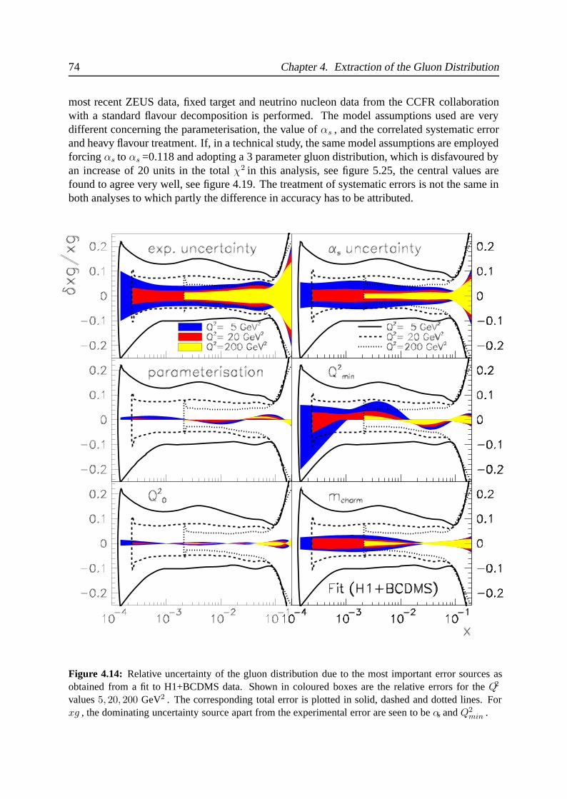
74 Chapter 4. Extraction of the Gluon Distribution
most recent ZEUS data, fixed target and neutrino nucleon data from the CCFR collaborationwith a standard flavour decomposition is performed. The model assumptions used are verydifferent concerning the parameterisation, the value of αs , and the correlated systematic errorand heavy flavour treatment. If, in a technical study, the same model assumptions are employedforcing αs to αs =0.118 and adopting a 3 parameter gluon distribution, which is disfavoured byan increase of 20 units in the total χ2 in this analysis, see figure 5.25, the central values arefound to agree very well, see figure 4.19. The treatment of systematic errors is not the same inboth analyses to which partly the difference in accuracy has to be attributed.
Figure 4.14: Relative uncertainty of the gluon distribution due to the most important error sources asobtained from a fit to H1+BCDMS data. Shown in coloured boxes are the relative errors for the Q2
values 5, 20, 200 GeV2 . The corresponding total error is plotted in solid, dashed and dotted lines. Forxg , the dominating uncertainty source apart from the experimental error are seen to be αs and Q2
min .
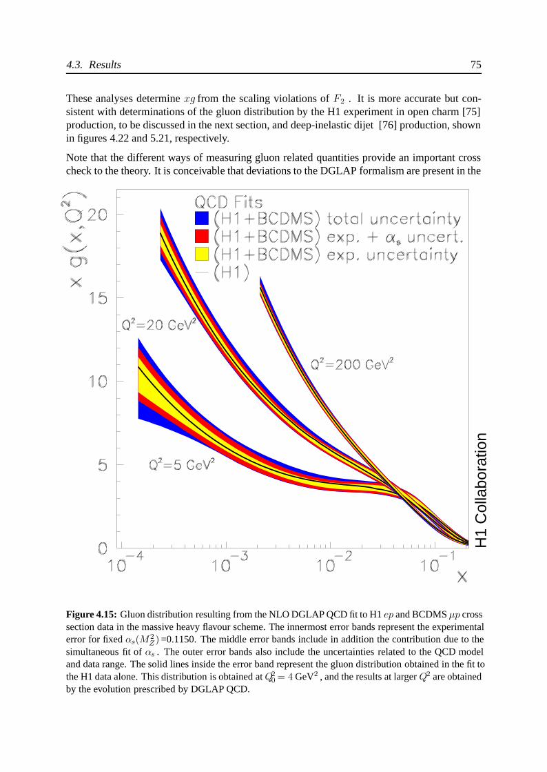
4.3. Results 75
These analyses determine xg from the scaling violations of F2 . It is more accurate but con-sistent with determinations of the gluon distribution by the H1 experiment in open charm [75]production, to be discussed in the next section, and deep-inelastic dijet [76] production, shownin figures 4.22 and 5.21, respectively.
Note that the different ways of measuring gluon related quantities provide an important crosscheck to the theory. It is conceivable that deviations to the DGLAP formalism are present in the
H1
Col
labo
ratio
n
Figure 4.15: Gluon distribution resulting from the NLO DGLAP QCD fit to H1 ep and BCDMS μp crosssection data in the massive heavy flavour scheme. The innermost error bands represent the experimentalerror for fixed αs(M2
Z) =0.1150. The middle error bands include in addition the contribution due to thesimultaneous fit of αs . The outer error bands also include the uncertainties related to the QCD modeland data range. The solid lines inside the error band represent the gluon distribution obtained in the fit tothe H1 data alone. This distribution is obtained at Q2
0 = 4 GeV2 , and the results at larger Q2 are obtainedby the evolution prescribed by DGLAP QCD.
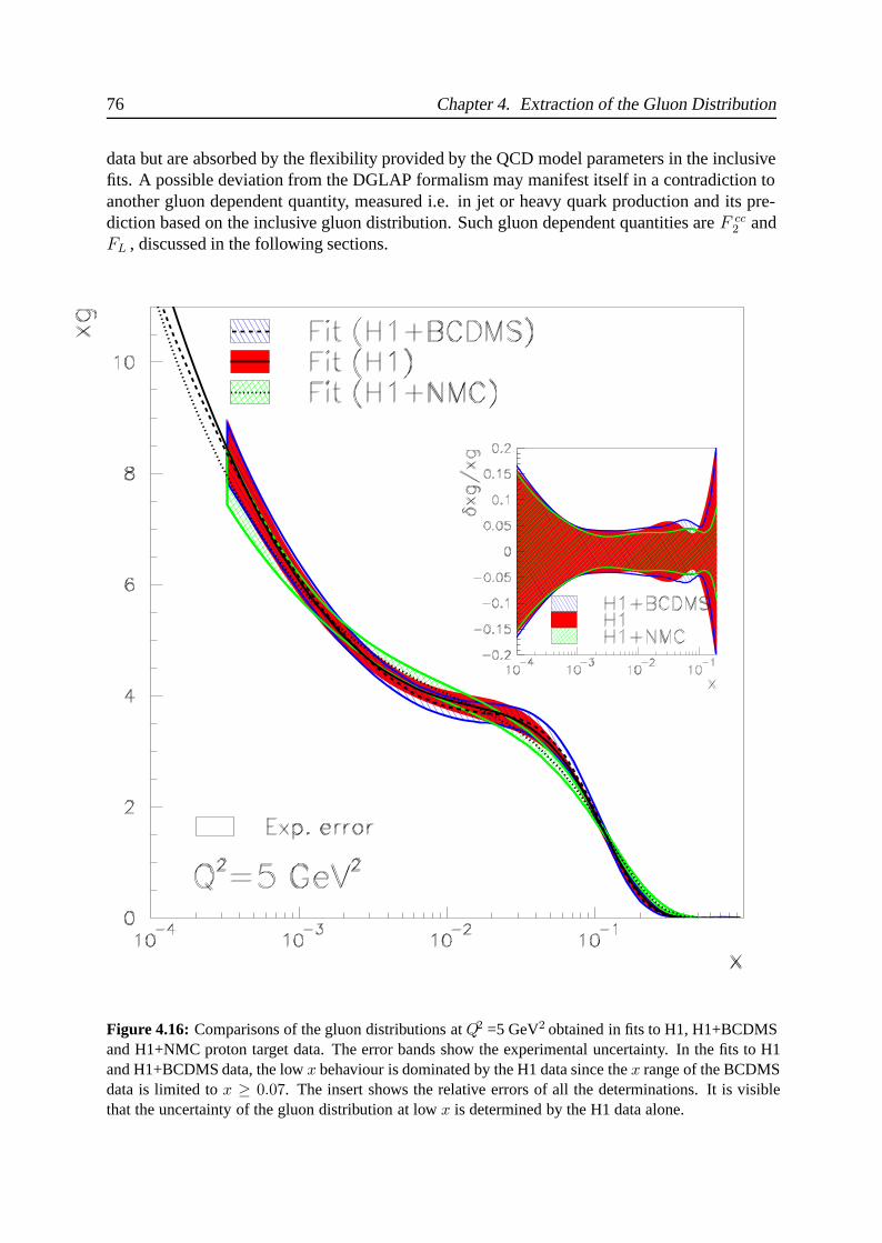
76 Chapter 4. Extraction of the Gluon Distribution
data but are absorbed by the flexibility provided by the QCD model parameters in the inclusivefits. A possible deviation from the DGLAP formalism may manifest itself in a contradiction toanother gluon dependent quantity, measured i.e. in jet or heavy quark production and its pre-diction based on the inclusive gluon distribution. Such gluon dependent quantities are F cc
2 andFL , discussed in the following sections.
Figure 4.16: Comparisons of the gluon distributions at Q2 =5 GeV2 obtained in fits to H1, H1+BCDMSand H1+NMC proton target data. The error bands show the experimental uncertainty. In the fits to H1and H1+BCDMS data, the low x behaviour is dominated by the H1 data since the x range of the BCDMSdata is limited to x ≥ 0.07. The insert shows the relative errors of all the determinations. It is visiblethat the uncertainty of the gluon distribution at low x is determined by the H1 data alone.
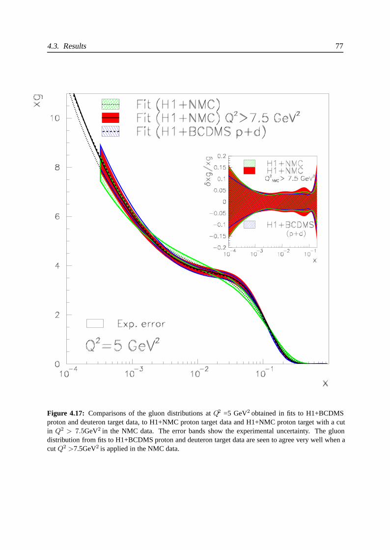
4.3. Results 77
Figure 4.17: Comparisons of the gluon distributions at Q2 =5 GeV2 obtained in fits to H1+BCDMSproton and deuteron target data, to H1+NMC proton target data and H1+NMC proton target with a cutin Q2 > 7.5GeV2 in the NMC data. The error bands show the experimental uncertainty. The gluondistribution from fits to H1+BCDMS proton and deuteron target data are seen to agree very well when acut Q2 >7.5GeV2 is applied in the NMC data.
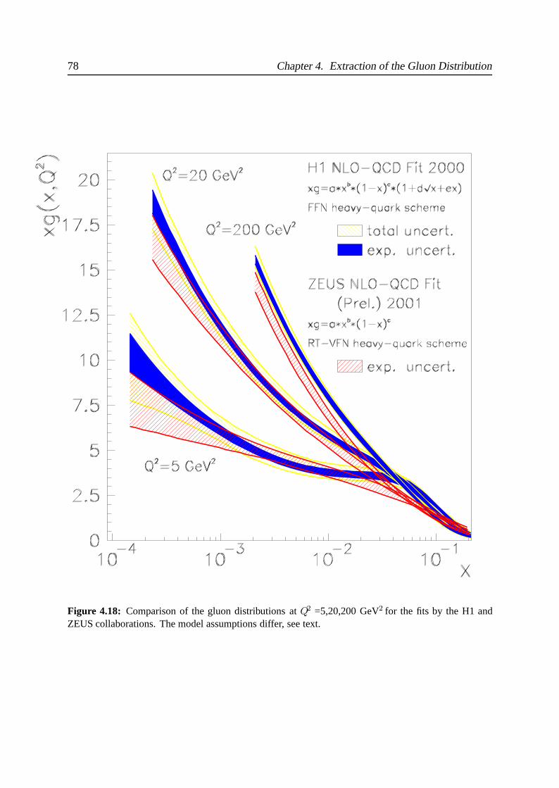
78 Chapter 4. Extraction of the Gluon Distribution
Figure 4.18: Comparison of the gluon distributions at Q2 =5,20,200 GeV2 for the fits by the H1 andZEUS collaborations. The model assumptions differ, see text.
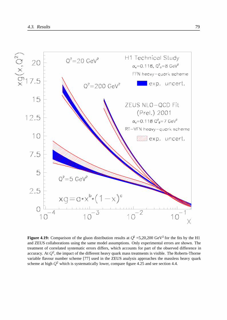
4.3. Results 79
Figure 4.19: Comparison of the gluon distribution results at Q2 =5,20,200 GeV2 for the fits by the H1and ZEUS collaborations using the same model assumptions. Only experimental errors are shown. Thetreatment of correlated systematic errors differs, which accounts for part of the observed difference inaccuracy. At Q2, the impact of the different heavy quark mass treatments is visible. The Roberts-Thornevariable flavour number scheme [77] used in the ZEUS analysis approaches the massless heavy quarkscheme at high Q2 which is systematically lower, compare figure 4.25 and see section 4.4.
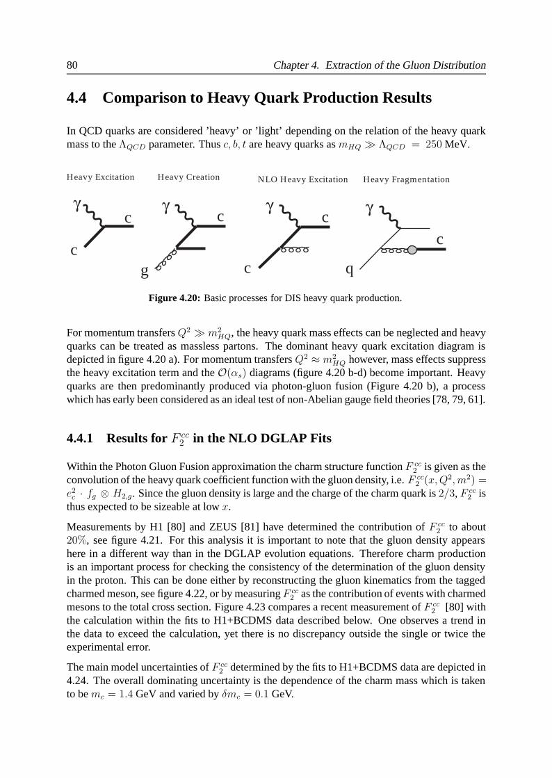
80 Chapter 4. Extraction of the Gluon Distribution
4.4 Comparison to Heavy Quark Production Results
In QCD quarks are considered ’heavy’ or ’light’ depending on the relation of the heavy quarkmass to the ΛQCD parameter. Thus c, b, t are heavy quarks as mHQ � ΛQCD = 250 MeV.
γ γ γγ
cc
ccc
g c q
Heavy Excitation Heavy Creation NLO Heavy Excitation Heavy Fragmentation
Figure 4.20: Basic processes for DIS heavy quark production.
For momentum transfers Q2 � m2HQ, the heavy quark mass effects can be neglected and heavy
quarks can be treated as massless partons. The dominant heavy quark excitation diagram isdepicted in figure 4.20 a). For momentum transfers Q2 ≈ m2
HQ however, mass effects suppressthe heavy excitation term and the O(αs) diagrams (figure 4.20 b-d) become important. Heavyquarks are then predominantly produced via photon-gluon fusion (Figure 4.20 b), a processwhich has early been considered as an ideal test of non-Abelian gauge field theories [78, 79, 61].
4.4.1 Results for F cc2 in the NLO DGLAP Fits
Within the Photon Gluon Fusion approximation the charm structure function F cc2 is given as the
convolution of the heavy quark coefficient function with the gluon density, i.e. F cc2 (x, Q2, m2) =
e2c · fg ⊗ H2,g. Since the gluon density is large and the charge of the charm quark is 2/3, F cc
2 isthus expected to be sizeable at low x.
Measurements by H1 [80] and ZEUS [81] have determined the contribution of F cc2 to about
20%, see figure 4.21. For this analysis it is important to note that the gluon density appearshere in a different way than in the DGLAP evolution equations. Therefore charm productionis an important process for checking the consistency of the determination of the gluon densityin the proton. This can be done either by reconstructing the gluon kinematics from the taggedcharmed meson, see figure 4.22, or by measuring F cc
2 as the contribution of events with charmedmesons to the total cross section. Figure 4.23 compares a recent measurement of F cc
2 [80] withthe calculation within the fits to H1+BCDMS data described below. One observes a trend inthe data to exceed the calculation, yet there is no discrepancy outside the single or twice theexperimental error.
The main model uncertainties of F cc2 determined by the fits to H1+BCDMS data are depicted in
4.24. The overall dominating uncertainty is the dependence of the charm mass which is takento be mc = 1.4 GeV and varied by δmc = 0.1 GeV.
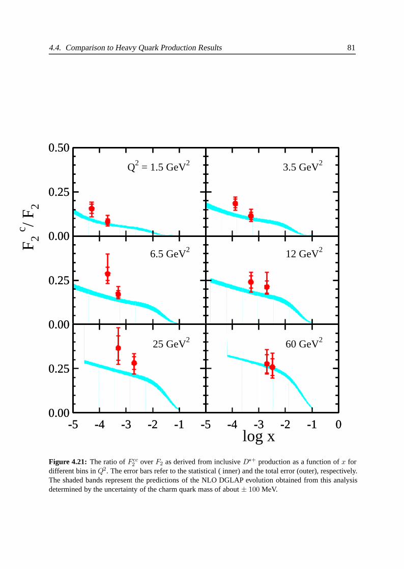
4.4. Comparison to Heavy Quark Production Results 81
0.00
0.25
0.50
Q2 = 1.5 GeV2
0.00
0.25
0.50
3.5 GeV2
0.00
0.25
6.5 GeV2
0.00
0.25
12 GeV2
-5 -4 -3 -2 -10.00
0.25
25 GeV2
-5 -4 -3 -2 -10.00
0.25
-5 -4 -3 -2 -1 0
60 GeV2
log x
F 2 c / F
2
-5 -4 -3 -2 -1 0
Figure 4.21: The ratio of Fcc2 over F2 as derived from inclusive D�+ production as a function of x for
different bins in Q2. The error bars refer to the statistical ( inner) and the total error (outer), respectively.The shaded bands represent the predictions of the NLO DGLAP evolution obtained from this analysisdetermined by the uncertainty of the charm quark mass of about ± 100 MeV.
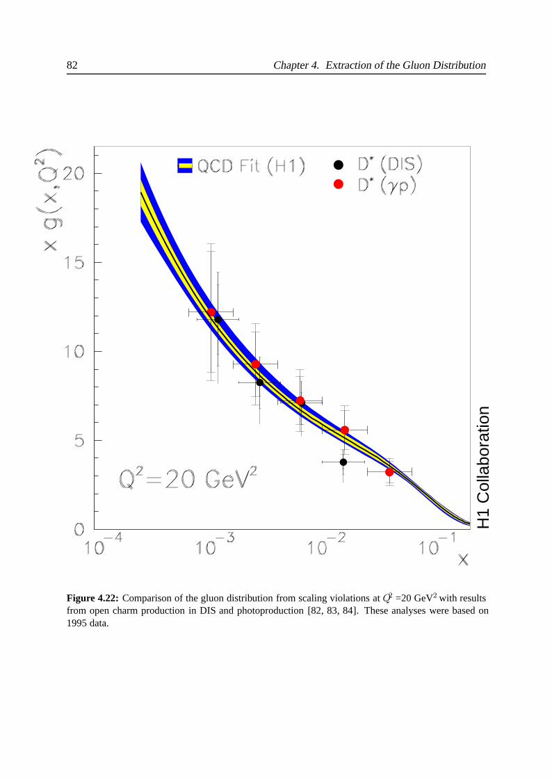
82 Chapter 4. Extraction of the Gluon Distribution
H1
Col
labo
ratio
n
Figure 4.22: Comparison of the gluon distribution from scaling violations at Q2 =20 GeV2 with resultsfrom open charm production in DIS and photoproduction [82, 83, 84]. These analyses were based on1995 data.
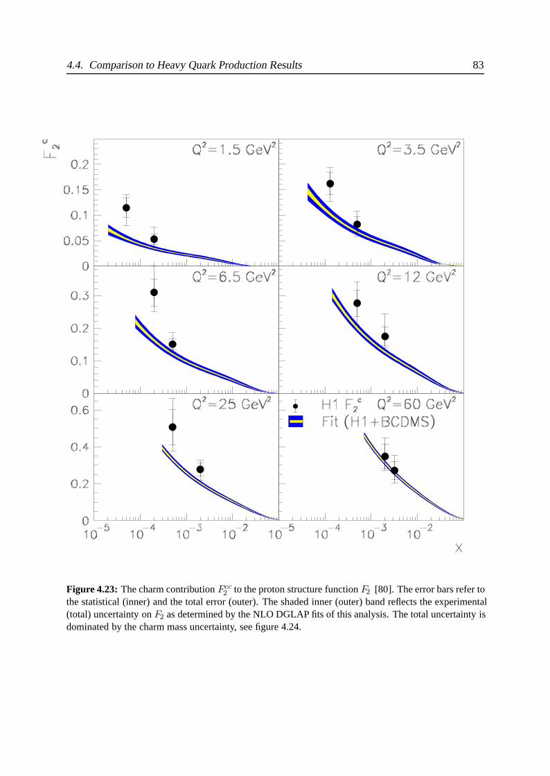
4.4. Comparison to Heavy Quark Production Results 83
Figure 4.23: The charm contribution Fcc2 to the proton structure function F2 [80]. The error bars refer to
the statistical (inner) and the total error (outer). The shaded inner (outer) band reflects the experimental(total) uncertainty on F2 as determined by the NLO DGLAP fits of this analysis. The total uncertainty isdominated by the charm mass uncertainty, see figure 4.24.
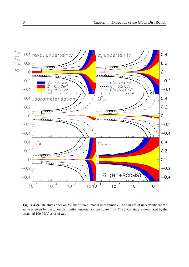
84 Chapter 4. Extraction of the Gluon Distribution
Figure 4.24: Relative errors on Fcc2 by different model uncertainties. The sources of uncertainty are the
same as given for the gluon distribution uncertainty, see figure 4.14. The uncertainty is dominated by theassumed 100 MeV error of mc.
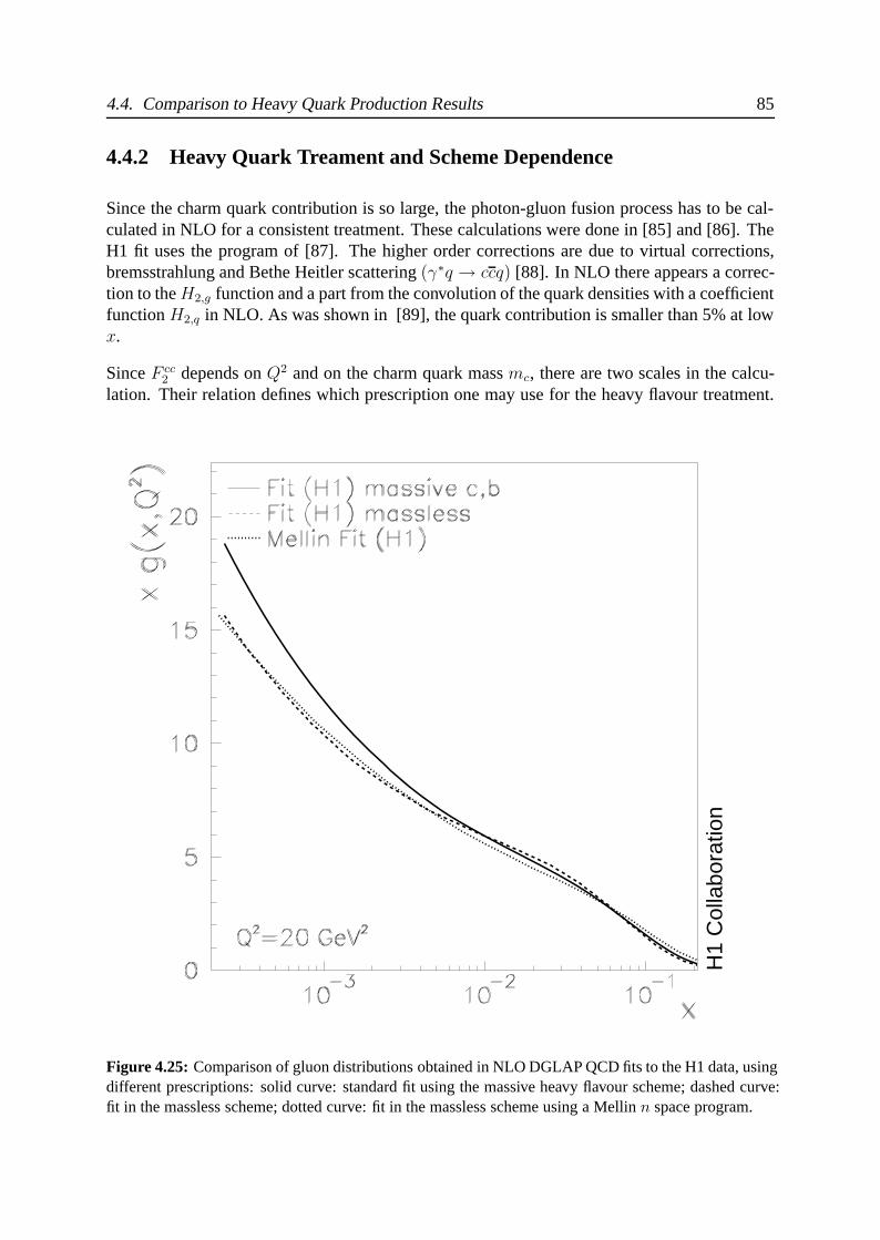
4.4. Comparison to Heavy Quark Production Results 85
4.4.2 Heavy Quark Treament and Scheme Dependence
Since the charm quark contribution is so large, the photon-gluon fusion process has to be cal-culated in NLO for a consistent treatment. These calculations were done in [85] and [86]. TheH1 fit uses the program of [87]. The higher order corrections are due to virtual corrections,bremsstrahlung and Bethe Heitler scattering (γ∗q → ccq) [88]. In NLO there appears a correc-tion to the H2,g function and a part from the convolution of the quark densities with a coefficientfunction H2,q in NLO. As was shown in [89], the quark contribution is smaller than 5% at lowx.
Since F cc2 depends on Q2 and on the charm quark mass mc, there are two scales in the calcu-
lation. Their relation defines which prescription one may use for the heavy flavour treatment.
H1
Col
labo
ratio
n
Figure 4.25: Comparison of gluon distributions obtained in NLO DGLAP QCD fits to the H1 data, usingdifferent prescriptions: solid curve: standard fit using the massive heavy flavour scheme; dashed curve:fit in the massless scheme; dotted curve: fit in the massless scheme using a Mellin n space program.

86 Chapter 4. Extraction of the Gluon Distribution
Near the charm production threshold, one considers three light flavours, i.e. the proton to con-sist of three light quarks u, d, s and the gluon, while charm quarks arise not from a proton charmquark distribution but via photon-gluon fusion. This is the massive flavour scheme or three fixedflavour number scheme (3FFNS). Away from the threshold, one considers 4 light quarks with4 parton densities which defines the four fixed flavour number scheme (4FFNS) which is alsocalled the massless scheme.
In 1997 an attempt was made to define a procedure which interpolates between these fixedflavour number schemes and which are called variable flavour number schemes (VFNS). Inleading order this was done by [90] and a higher order generalisation was considered [91]. TheMRST group introduced a smoothness derivative criterion which leads to a similar, but distinctsolution of this problem [92].
The charm structure function calculated in QCD depends on the treatment of charm, and so doesthe gluon distribution. These quantities are thus only defined in a theoretical context. The sameis true for bottom quarks which, however, contribute only at the per cent level to the inclusivescattering cross section. In this analysis, the 3FFNS scheme is used, treating u, d, s as lightquarks and the charm and bottom quarks as heavy in next-to-leading order.
The dependence of the gluon distribution on the heavy quark treatment is depicted in figure 4.25.If the massive quark description for charm and beauty production is replaced by the masslesstreatment of heavy quarks, the gluon distribution changes as illustrated. The gluon distributionin the massless fit is about 15% lower at small x as compared to the standard result. A consistentcross check of this massless fit result is obtained with a QCD evolution program based on theMellin n space technique [93]. This technique provides an alternative solution to the DGLAPevolution of massless quarks, solving the convolution integrals by reducing them to simpleproducts via Mellin transformations.
4.5 QCD Prediction for FL(x, Q2) and its Uncertainties
Another quantity with complementary information about the gluon distribution is the longitu-dinal structure function FL which leads to a damping effect of the reduced double differentialcross section σr towards low x, as can be seen in figure 4.26. Effects related to FL become ap-preciable only at highest y > 0.6, since FL enters the cross section with a kinematical weightingfactor proportional to y2. This is a tiny fraction of the logarithmic phase space of the H1 data inx and Q2 as can be seen in figure 2.2.
The QCD fit to the H1 F2 data allows a prediction to be made for the longitudinal structurefunction. FL(x, Q2) is closely related to the gluon distribution, see equations 1.21 and 1.22.To order O(αs ), an approximate relation [94] similar to the approximation 4.1 for xg can beobtained for FL(x, Q2) :
xg(x, Q2) =3
5·[
3π
4αsFL(0.4x, Q2) − 1
2· F2(0.8x, Q2)
], (4.2)
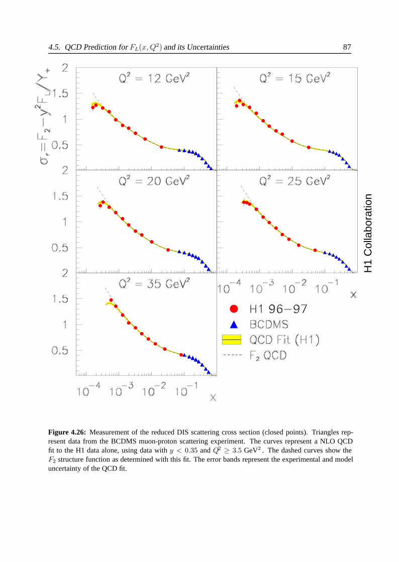
4.5. QCD Prediction for FL(x, Q2) and its Uncertainties 87
H1
Col
labo
ratio
n
Figure 4.26: Measurement of the reduced DIS scattering cross section (closed points). Triangles rep-resent data from the BCDMS muon-proton scattering experiment. The curves represent a NLO QCDfit to the H1 data alone, using data with y < 0.35 and Q2 ≥ 3.5 GeV2 . The dashed curves show theF2 structure function as determined with this fit. The error bands represent the experimental and modeluncertainty of the QCD fit.
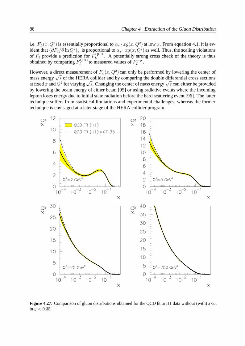
88 Chapter 4. Extraction of the Gluon Distribution
i.e. FL(x, Q2) is essentially proportional to αs · xg(x, Q2) at low x. From equation 4.1, it is ev-ident that (∂F2/∂ ln Q2)x is proportional to αs · xg(x, Q2) as well. Thus, the scaling violationsof F2 provide a prediction for F QCD
L . A potentially strong cross check of the theory is thusobtained by comparing F QCD
L to measured values of F expL .
However, a direct measurement of FL(x, Q2) can only be performed by lowering the center ofmass energy
√s of the HERA collider and by comparing the double differential cross sections
at fixed x and Q2 for varying√
s. Changing the center of mass energy√
s can either be providedby lowering the beam energy of either beam [95] or using radiative events where the incominglepton loses energy due to initial state radiation before the hard scattering event [96]. The lattertechnique suffers from statistical limitations and experimental challenges, whereas the formertechnique is envisaged at a later stage of the HERA collider program.
Figure 4.27: Comparison of gluon distributions obtained for the QCD fit to H1 data without (with) a cutin y < 0.35.
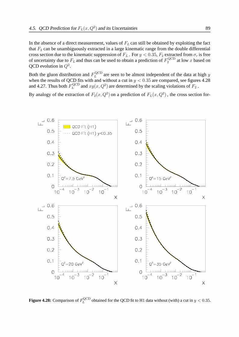
4.5. QCD Prediction for FL(x, Q2) and its Uncertainties 89
In the absence of a direct measurement, values of FL can still be obtained by exploiting the factthat F2 can be unambiguously extracted in a large kinematic range from the double differentialcross section due to the kinematic suppression of FL . For y < 0.35, F2 extracted from σr is freeof uncertainty due to FL and thus can be used to obtain a prediction of F QCD
2 at low x based onQCD evolution in Q2.
Both the gluon distribution and F QCDL are seen to be almost independent of the data at high y
when the results of QCD fits with and without a cut in y < 0.35 are compared, see figures 4.28and 4.27. Thus both F QCD
L and xg(x, Q2) are determined by the scaling violations of F2 .
By analogy of the extraction of F2(x, Q2) on a prediction of FL(x, Q2) , the cross section for-
Figure 4.28: Comparison of FQCDL obtained for the QCD fit to H1 data without (with) a cut in y < 0.35.
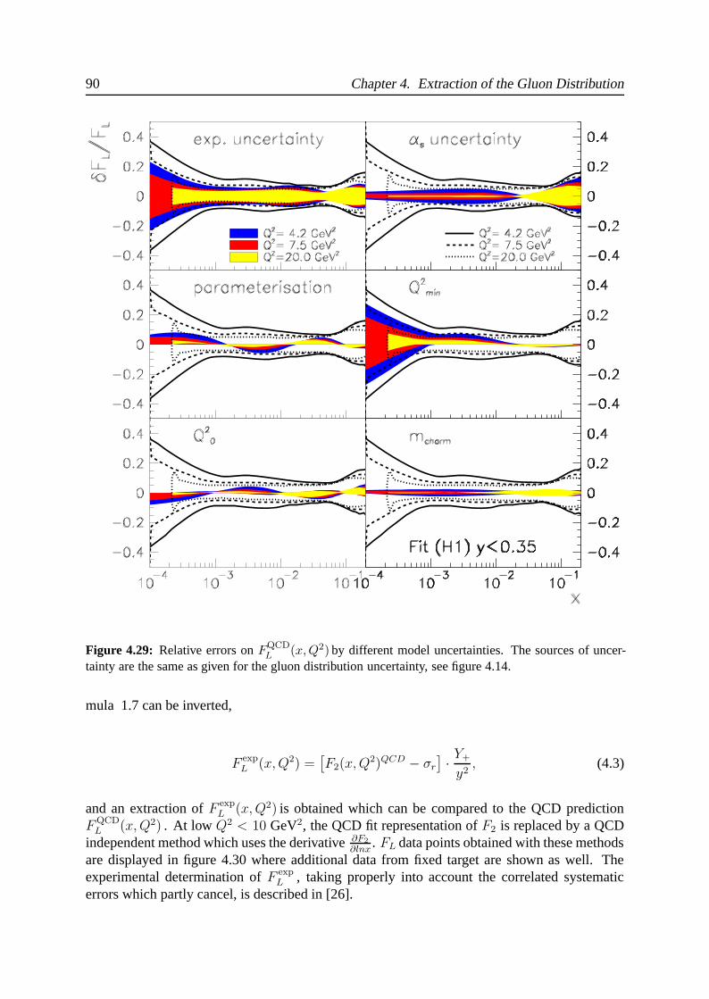
90 Chapter 4. Extraction of the Gluon Distribution
Figure 4.29: Relative errors on FQCDL (x,Q2) by different model uncertainties. The sources of uncer-
tainty are the same as given for the gluon distribution uncertainty, see figure 4.14.
mula 1.7 can be inverted,
F expL (x, Q2) =
[F2(x, Q2)QCD − σr
] · Y+
y2, (4.3)
and an extraction of F expL (x, Q2) is obtained which can be compared to the QCD prediction
FQCDL (x, Q2) . At low Q2 < 10 GeV2, the QCD fit representation of F2 is replaced by a QCD
independent method which uses the derivative ∂F2
∂lnx. FL data points obtained with these methods
are displayed in figure 4.30 where additional data from fixed target are shown as well. Theexperimental determination of F exp
L , taking properly into account the correlated systematicerrors which partly cancel, is described in [26].
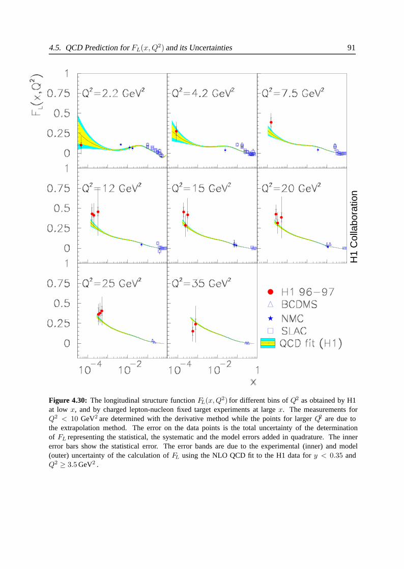
4.5. QCD Prediction for FL(x, Q2) and its Uncertainties 91
H1
Col
labo
ratio
n
Figure 4.30: The longitudinal structure function FL(x,Q2) for different bins of Q2 as obtained by H1at low x, and by charged lepton-nucleon fixed target experiments at large x. The measurements forQ2 < 10 GeV2 are determined with the derivative method while the points for larger Q2 are due tothe extrapolation method. The error on the data points is the total uncertainty of the determinationof FL representing the statistical, the systematic and the model errors added in quadrature. The innererror bars show the statistical error. The error bands are due to the experimental (inner) and model(outer) uncertainty of the calculation of FL using the NLO QCD fit to the H1 data for y < 0.35 andQ2 ≥ 3.5 GeV2 .
92 Chapter 4. Extraction of the Gluon Distribution
The QCD fit, similarly as for xg , allows the longitudinal structure function to be predicted witha certain accuracy limited by the experimental and model uncertainties. The error bands in 4.30reflect these uncertainties in the QCD analysis to H1 data with a cut in y < 0.35. The largesteffects are seen to result from the experimental errors and from the adopted minimum value ofQ2 used in the analysis while the uncertainty due to αs, the charm mass and the parameterisa-tions are small. Figure 4.30 compares the QCD fit prediction with the data points obtained fromthe H1 data as well as from fixed target experiments. At the present level of accuracy, the dataare consistent with the QCD calculation to order O(α2
s) obtained from the QCD fit.
The net uncertainties at smallest x are large because the fit is restricted to y < 0.35 in orderto become independent of FL. If the fit is extended to the highest y, or smallest x, region, theuncertainty becomes nearly twice smaller at low x. Then, however, the FL data themselves arepotentially influencing the fit and the comparison of the extracted FL data points [26, 27] withthe QCD prediction becomes conceptionally less convincing.
Chapter 5
Determination of αs(M2Z)
The strong coupling constant αs is the only fundamental free parameter of QCD. It is there-fore not surprising that it enters the computation of many observables in QCD. However, inpractice αs is correlated with other phenomenological parameters of the theory, which accountfor the non-perturbative part of the theory, in particular with the x dependence of the partondistributions.
Deep inelastic lepton nucleon scattering has been an ideal testing ground for determining αs
since the theory is probed at high momentum transfers where QCD is asymptotically free andthe theory well formulated up to higher orders in perturbation theory. The determination of thestrong coupling constant in this analysis uses the DGLAP equations to NLO which govern thescaling violations of F2(x, Q2) and also of FL(x, Q2) .
A potential problem arises from the correlation of αs with the gluon distribution. This is re-solved here by using high precision data at low x and high x. While the scaling violations atlow x are proportional to αs ·xg , in the valence quark region at high x they are predominantlydetermined by αs alone since the non-singlet evolution is independent of xg . Employing thenew precision data of H1 at low x and the BCDMS data at high x , both the non-singlet (highx ) as well as the singlet (low x ) sector of the DGLAP equations are well constrained. This isdemonstrated to determine αs and to disentangle its correlation with xg .
5.1 αs(M2Z) from a Fit to H1 and BCDMS Data
The fit to the H1 data alone determines αs(M2Z) to be 0.115 with an experimental error of
±0.005. This is the first measurement of αs with HERA inclusive cross section data alone.The precision of the large x, high Q2 H1 data [37] however is not sufficient to enable a com-petitive determination of αs(M
2Z) and of the gluon distribution simultaneously from the H1 data
alone. The most precise measurement of the DIS inclusive cross section at large x was obtainedby the BCDMS μp scattering experiment [97] (figure 4.3). These data are therefore combinedwith the H1 measurements.
93
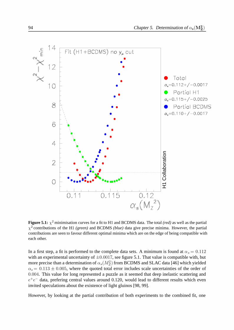
94 Chapter 5. Determination of αs(M2Z)
H1
Col
labo
ratio
n
Figure 5.1: χ2 minimisation curves for a fit to H1 and BCDMS data. The total (red) as well as the partialχ2 contributions of the H1 (green) and BCDMS (blue) data give precise minima. However, the partialcontributions are seen to favour different optimal minima which are on the edge of being compatible witheach other.
In a first step, a fit is performed to the complete data sets. A minimum is found at αs = 0.112with an experimental uncertainty of ±0.0017, see figure 5.1. That value is compatible with, butmore precise than a determination of αs(M
2Z) from BCDMS and SLAC data [46] which yielded
αs = 0.113 ± 0.005, where the quoted total error includes scale uncertainties of the order of0.004. This value for long represented a puzzle as it seemed that deep inelastic scattering ande+e− data, prefering central values around 0.120, would lead to different results which eveninvited speculations about the existence of light gluinos [98, 99].
However, by looking at the partial contribution of both experiments to the combined fit, one
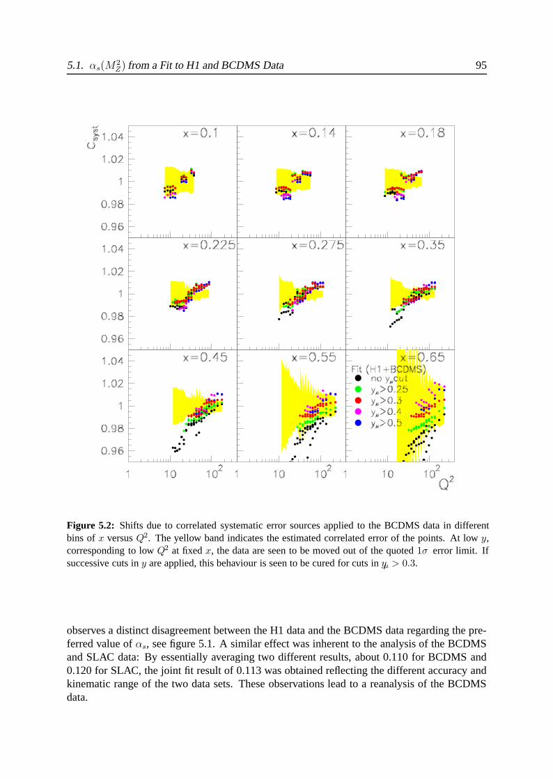
5.1. αs(M2Z) from a Fit to H1 and BCDMS Data 95
Figure 5.2: Shifts due to correlated systematic error sources applied to the BCDMS data in differentbins of x versus Q2. The yellow band indicates the estimated correlated error of the points. At low y,corresponding to low Q2 at fixed x, the data are seen to be moved out of the quoted 1σ error limit. Ifsuccessive cuts in y are applied, this behaviour is seen to be cured for cuts in yμ > 0.3.
observes a distinct disagreement between the H1 data and the BCDMS data regarding the pre-ferred value of αs, see figure 5.1. A similar effect was inherent to the analysis of the BCDMSand SLAC data: By essentially averaging two different results, about 0.110 for BCDMS and0.120 for SLAC, the joint fit result of 0.113 was obtained reflecting the different accuracy andkinematic range of the two data sets. These observations lead to a reanalysis of the BCDMSdata.
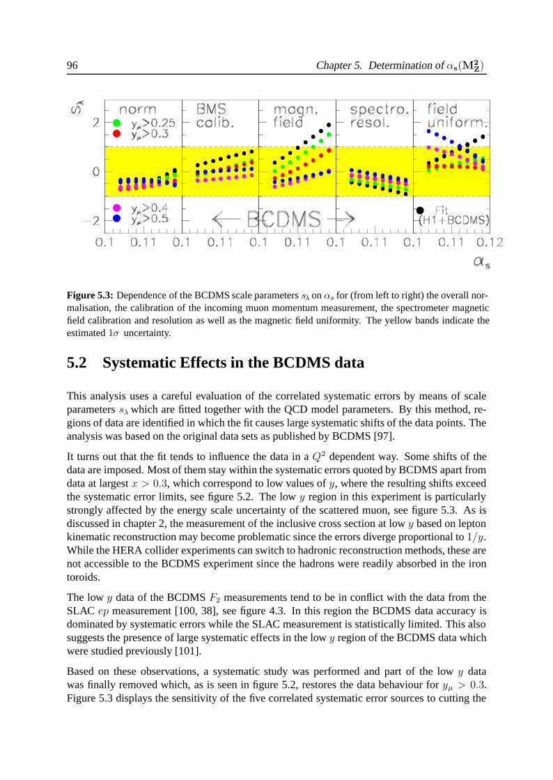
96 Chapter 5. Determination of αs(M2Z)
Figure 5.3: Dependence of the BCDMS scale parameters sλ on αs for (from left to right) the overall nor-malisation, the calibration of the incoming muon momentum measurement, the spectrometer magneticfield calibration and resolution as well as the magnetic field uniformity. The yellow bands indicate theestimated 1σ uncertainty.
5.2 Systematic Effects in the BCDMS data
This analysis uses a careful evaluation of the correlated systematic errors by means of scaleparameters sλ which are fitted together with the QCD model parameters. By this method, re-gions of data are identified in which the fit causes large systematic shifts of the data points. Theanalysis was based on the original data sets as published by BCDMS [97].
It turns out that the fit tends to influence the data in a Q2 dependent way. Some shifts of thedata are imposed. Most of them stay within the systematic errors quoted by BCDMS apart fromdata at largest x > 0.3, which correspond to low values of y, where the resulting shifts exceedthe systematic error limits, see figure 5.2. The low y region in this experiment is particularlystrongly affected by the energy scale uncertainty of the scattered muon, see figure 5.3. As isdiscussed in chapter 2, the measurement of the inclusive cross section at low y based on leptonkinematic reconstruction may become problematic since the errors diverge proportional to 1/y.While the HERA collider experiments can switch to hadronic reconstruction methods, these arenot accessible to the BCDMS experiment since the hadrons were readily absorbed in the irontoroids.
The low y data of the BCDMS F2 measurements tend to be in conflict with the data from theSLAC ep measurement [100, 38], see figure 4.3. In this region the BCDMS data accuracy isdominated by systematic errors while the SLAC measurement is statistically limited. This alsosuggests the presence of large systematic effects in the low y region of the BCDMS data whichwere studied previously [101].
Based on these observations, a systematic study was performed and part of the low y datawas finally removed which, as is seen in figure 5.2, restores the data behaviour for yμ > 0.3.Figure 5.3 displays the sensitivity of the five correlated systematic error sources to cutting the
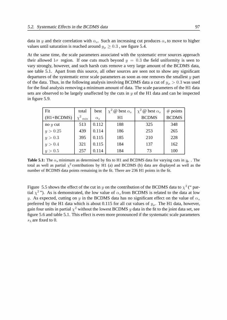
5.2. Systematic Effects in the BCDMS data 97
data in y and their correlation with αs. Such an increasing cut produces αs to move to highervalues until saturation is reached around yμ ≥ 0.3 , see figure 5.4.
At the same time, the scale parameters associated with the systematic error sources approachtheir allowed 1σ region. If one cuts much beyond y = 0.3 the field uniformity is seen tovary strongly, however, and such harsh cuts remove a very large amount of the BCDMS data,see table 5.1. Apart from this source, all other sources are seen not to show any significantdepartures of the systematic error scale parameters as soon as one removes the smallest y partof the data. Thus, in the following analysis involving BCDMS data a cut of yμ > 0.3 was usedfor the final analysis removing a minimum amount of data. The scale parameters of the H1 datasets are observed to be largely unaffected by the cuts in y of the H1 data and can be inspectedin figure 5.9.
Fit total best χ2 @ best αs χ2 @ best αs # points
(H1+BCDMS) χ2min αs H1 BCDMS BCDMS
no y cut 513 0.112 188 325 348
y > 0.25 439 0.114 186 253 265
y > 0.3 395 0.115 185 210 228
y > 0.4 321 0.115 184 137 162
y > 0.5 257 0.114 184 73 100
Table 5.1: The αs minimum as determined by fits to H1 and BCDMS data for varying cuts in yμ . Thetotal as well as partial χ2 contributions by H1 (a) and BCDMS (b) data are displayed as well as thenumber of BCDMS data points remaining in the fit. There are 236 H1 points in the fit.
Figure 5.5 shows the effect of the cut in y on the contribution of the BCDMS data to χ2 (“ par-tial χ2 ”). As is demonstrated, the low value of αs from BCDMS is related to the data at lowy. As expected, cutting on y in the BCDMS data has no significant effect on the value of αs
preferred by the H1 data which is about 0.115 for all cut values of yμ. The H1 data, however,gain four units in partial χ2 without the lowest BCDMS y data in the fit to the joint data set, seefigure 5.6 and table 5.1. This effect is even more pronounced if the systematic scale parameterssλ are fixed to 0.
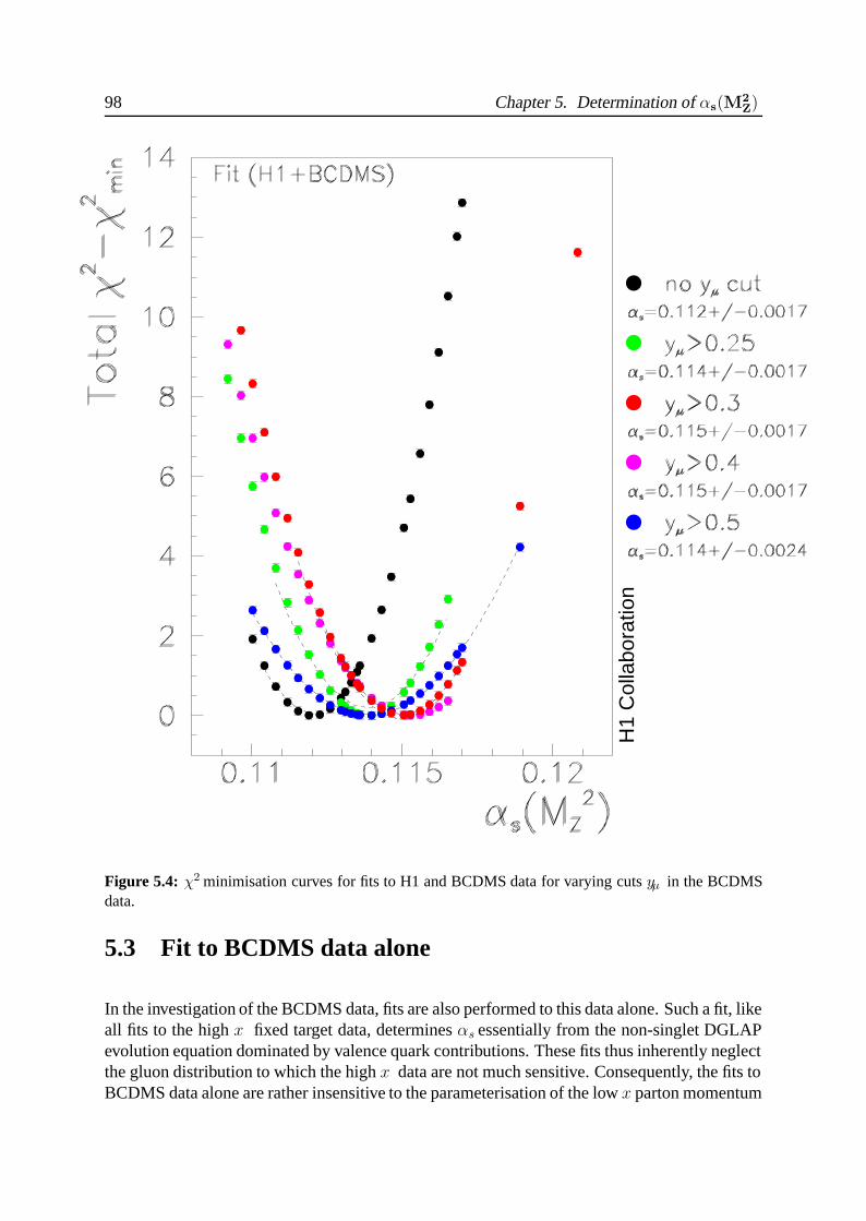
98 Chapter 5. Determination of αs(M2Z)
H1
Col
labo
ratio
n
Figure 5.4: χ2 minimisation curves for fits to H1 and BCDMS data for varying cuts yμ in the BCDMSdata.
5.3 Fit to BCDMS data alone
In the investigation of the BCDMS data, fits are also performed to this data alone. Such a fit, likeall fits to the high x fixed target data, determines αs essentially from the non-singlet DGLAPevolution equation dominated by valence quark contributions. These fits thus inherently neglectthe gluon distribution to which the high x data are not much sensitive. Consequently, the fits toBCDMS data alone are rather insensitive to the parameterisation of the low x parton momentum
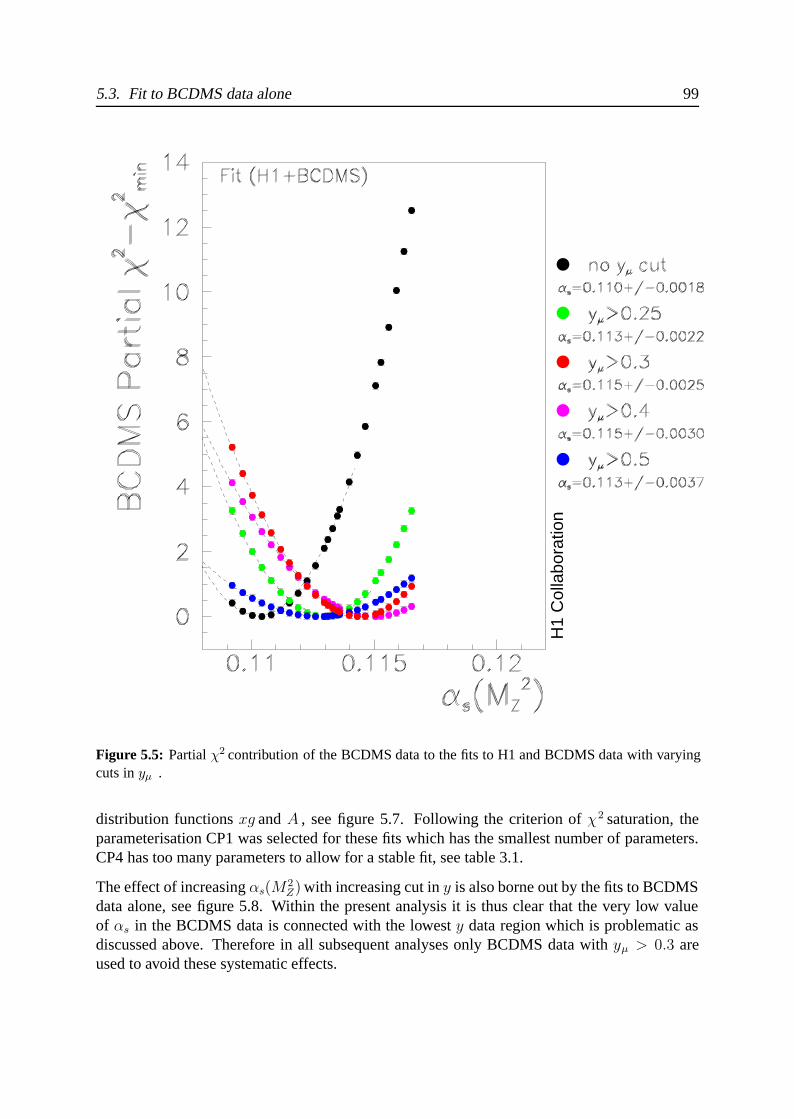
5.3. Fit to BCDMS data alone 99
H1
Col
labo
ratio
n
Figure 5.5: Partial χ2 contribution of the BCDMS data to the fits to H1 and BCDMS data with varyingcuts in yμ .
distribution functions xg and A , see figure 5.7. Following the criterion of χ2 saturation, theparameterisation CP1 was selected for these fits which has the smallest number of parameters.CP4 has too many parameters to allow for a stable fit, see table 3.1.
The effect of increasing αs(M2Z) with increasing cut in y is also borne out by the fits to BCDMS
data alone, see figure 5.8. Within the present analysis it is thus clear that the very low valueof αs in the BCDMS data is connected with the lowest y data region which is problematic asdiscussed above. Therefore in all subsequent analyses only BCDMS data with yμ > 0.3 areused to avoid these systematic effects.
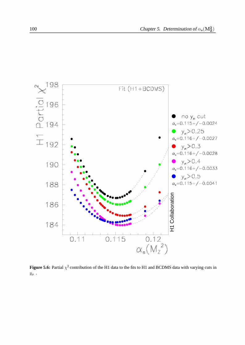
100 Chapter 5. Determination of αs(M2Z)
H1
Col
labo
ratio
n
Figure 5.6: Partial χ2 contribution of the H1 data to the fits to H1 and BCDMS data with varying cuts inyμ .
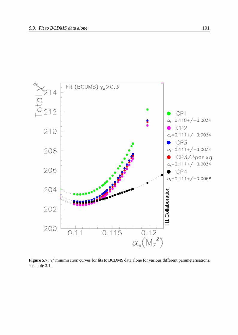
5.3. Fit to BCDMS data alone 101
H1
Col
labo
ratio
n
Figure 5.7: χ2 minimisation curves for fits to BCDMS data alone for various different parameterisations,see table 3.1.
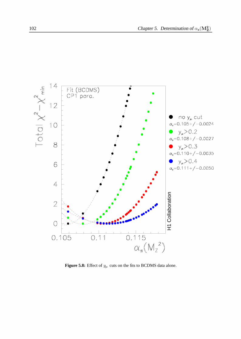
102 Chapter 5. Determination of αs(M2Z)
H1
Col
labo
ratio
n
Figure 5.8: Effect of yμ cuts on the fits to BCDMS data alone.
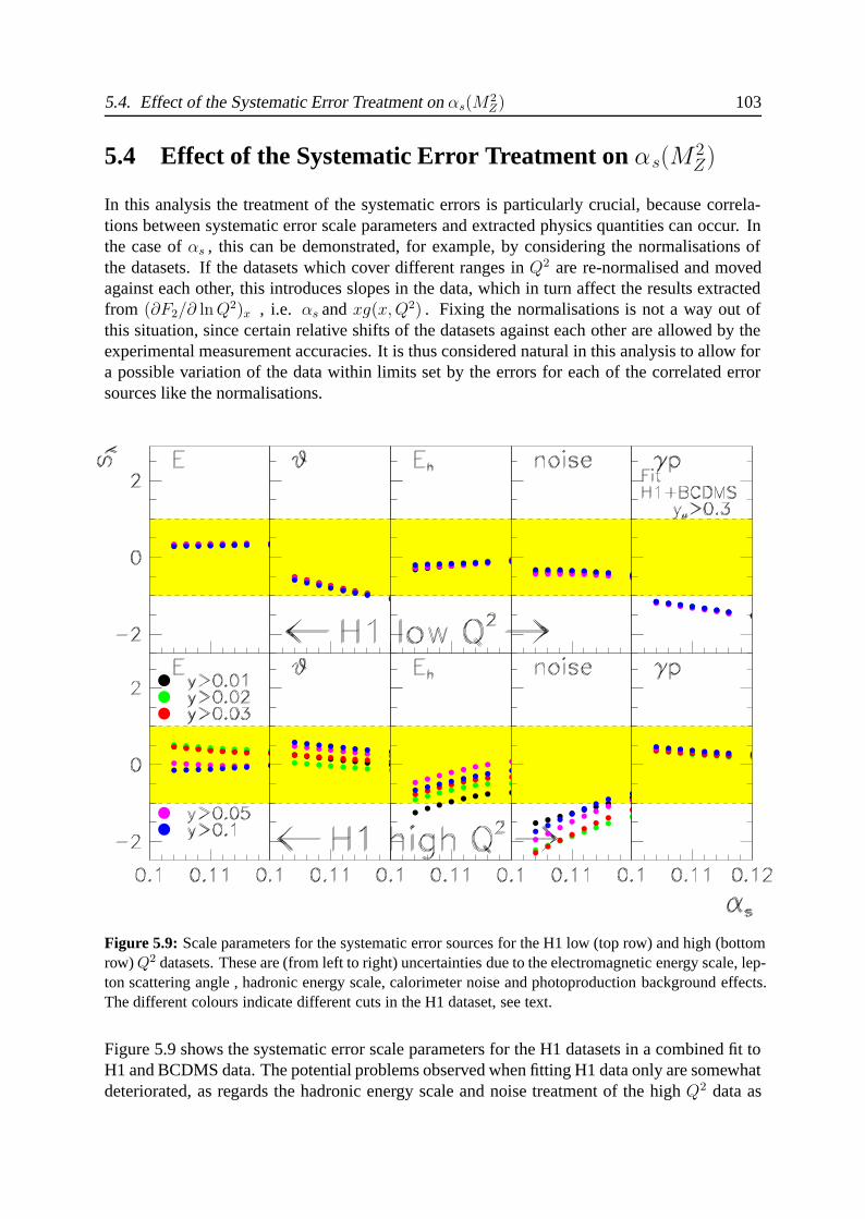
5.4. Effect of the Systematic Error Treatment on αs(M2Z) 103
5.4 Effect of the Systematic Error Treatment on αs(M2Z)
In this analysis the treatment of the systematic errors is particularly crucial, because correla-tions between systematic error scale parameters and extracted physics quantities can occur. Inthe case of αs , this can be demonstrated, for example, by considering the normalisations ofthe datasets. If the datasets which cover different ranges in Q2 are re-normalised and movedagainst each other, this introduces slopes in the data, which in turn affect the results extractedfrom (∂F2/∂ ln Q2)x , i.e. αs and xg(x, Q2) . Fixing the normalisations is not a way out ofthis situation, since certain relative shifts of the datasets against each other are allowed by theexperimental measurement accuracies. It is thus considered natural in this analysis to allow fora possible variation of the data within limits set by the errors for each of the correlated errorsources like the normalisations.
Figure 5.9: Scale parameters for the systematic error sources for the H1 low (top row) and high (bottomrow) Q2 datasets. These are (from left to right) uncertainties due to the electromagnetic energy scale, lep-ton scattering angle , hadronic energy scale, calorimeter noise and photoproduction background effects.The different colours indicate different cuts in the H1 dataset, see text.
Figure 5.9 shows the systematic error scale parameters for the H1 datasets in a combined fit toH1 and BCDMS data. The potential problems observed when fitting H1 data only are somewhatdeteriorated, as regards the hadronic energy scale and noise treatment of the high Q2 data as
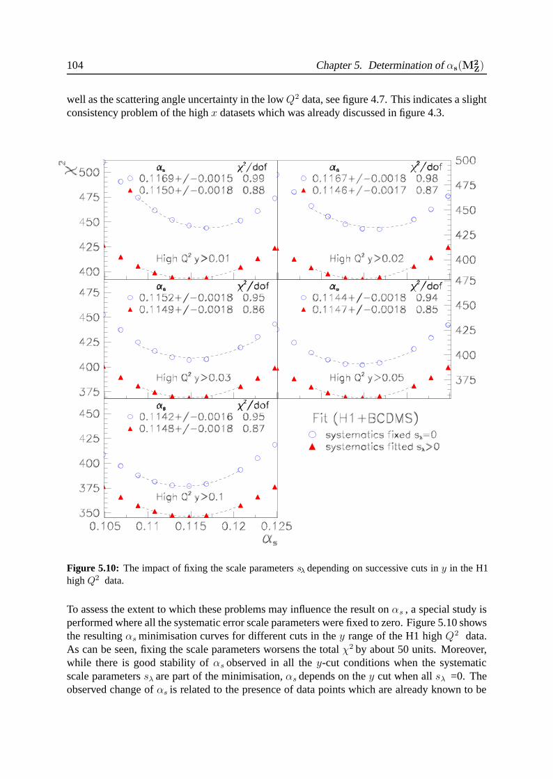
104 Chapter 5. Determination of αs(M2Z)
well as the scattering angle uncertainty in the low Q2 data, see figure 4.7. This indicates a slightconsistency problem of the high x datasets which was already discussed in figure 4.3.
Figure 5.10: The impact of fixing the scale parameters sλ depending on successive cuts in y in the H1high Q2 data.
To assess the extent to which these problems may influence the result on αs , a special study isperformed where all the systematic error scale parameters were fixed to zero. Figure 5.10 showsthe resulting αs minimisation curves for different cuts in the y range of the H1 high Q2 data.As can be seen, fixing the scale parameters worsens the total χ2 by about 50 units. Moreover,while there is good stability of αs observed in all the y-cut conditions when the systematicscale parameters sλ are part of the minimisation, αs depends on the y cut when all sλ =0. Theobserved change of αs is related to the presence of data points which are already known to be
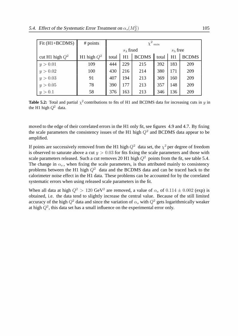
5.4. Effect of the Systematic Error Treatment on αs(M2Z) 105
Fit (H1+BCDMS) # points χ2min
sλ fixed sλ free
cut H1 high Q2 H1 high Q2 total H1 BCDMS total H1 BCDMS
y > 0.01 109 444 229 215 392 183 209
y > 0.02 100 430 216 214 380 171 209
y > 0.03 91 407 194 213 369 160 209
y > 0.05 78 390 177 213 357 148 209
y > 0.1 58 376 163 213 346 136 209
Table 5.2: Total and partial χ2 contributions to fits of H1 and BCDMS data for increasing cuts in y inthe H1 high Q2 data.
moved to the edge of their correlated errors in the H1 only fit, see figures 4.9 and 4.7. By fixingthe scale parameters the consistency issues of the H1 high Q2 and BCDMS data appear to beamplified.
If points are successively removed from the H1 high Q2 data set, the χ2 per degree of freedomis observed to saturate above a cut y > 0.03 for fits fixing the scale parameters and those withscale parameters released. Such a cut removes 20 H1 high Q2 points from the fit, see table 5.4.The change in αs , when fixing the scale parameters, is thus attributed mainly to consistencyproblems between the H1 high Q2 data and the BCDMS data and can be traced back to thecalorimeter noise effect in the H1 data. These problems can be accounted for by the correlatedsystematic errors when using released scale parameters in the fit.
When all data at high Q2 > 120 GeV2 are removed, a value of αs of 0.114 ± 0.002 (exp) isobtained, i.e. the data tend to slightly increase the central value. Because of the still limitedaccuracy of the high Q2 data and since the variation of αs with Q2 gets logarithmically weakerat high Q2, this data set has a small influence on the experimental error only.
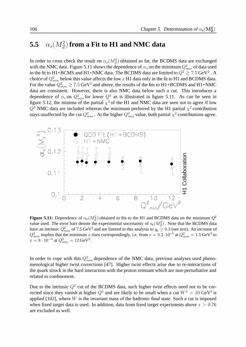
106 Chapter 5. Determination of αs(M2Z)
5.5 αs(M2Z) from a Fit to H1 and NMC data
In order to cross check the result on αs(M2Z) obtained so far, the BCDMS data are exchanged
with the NMC data. Figure 5.11 shows the dependence of αs on the minimum Q2min of data used
in the fit to H1+BCMS and H1+NMC data. The BCDMS data are limited to Q2 ≥ 7.5 GeV2 . Achoice of Q2
min below this value affects the low x H1 data only in the fit to H1 and BCDMS data.For the value Q2
min ≥ 7.5 GeV2 and above, the results of the fits to H1+BCDMS and H1+NMCdata are consistent. However, there is also NMC data below such a cut. This introduces adependence of αs on Q2
min for lower Q2 as is illustrated in figure 5.11. As can be seen infigure 5.12, the minima of the partial χ2 of the H1 and NMC data are seen not to agree if lowQ2 NMC data are included whereas the minimum preferred by the H1 partial χ2 contributionstays unaffected by the cut Q2
min . At the higher Q2min value, both partial χ2 contributions agree.
H1
Col
labo
ratio
n
Figure 5.11: Dependence of αs(M2Z) obtained in fits to the H1 and BCDMS data on the minimum Q2
value used. The error bars denote the experimental uncertainty of αs(M2Z) . Note that the BCDMS data
have an intrinsic Q2min of 7.5 GeV2 and are limited in this analysis to yμ ≥ 0.3 (see text). An increase of
Q2min implies that the minimum x rises correspondingly, i.e. from x = 3.2 ·10−5 at Q2
min = 1.5 GeV2 tox = 8 · 10−4 at Q2
min = 12 GeV2 .
In order to cope with this Q2min dependence of the NMC data, previous analyses used pheno-
menological higher twist corrections [47]. Higher twist effects arise due to re-interactions ofthe quark struck in the hard interaction with the proton remnant which are non-perturbative andrelated to confinement.
Due to the intrinsic Q2 cut of the BCDMS data, such higher twist effects need not to be cor-rected since they vanish at higher Q2 and are likely to be small when a cut W 2 > 10 GeV2 isapplied [102], where W is the invariant mass of the hadronic final state. Such a cut is imposedwhen fixed target data is used. In addition, data from fixed target experiments above x > 0.76are excluded as well.
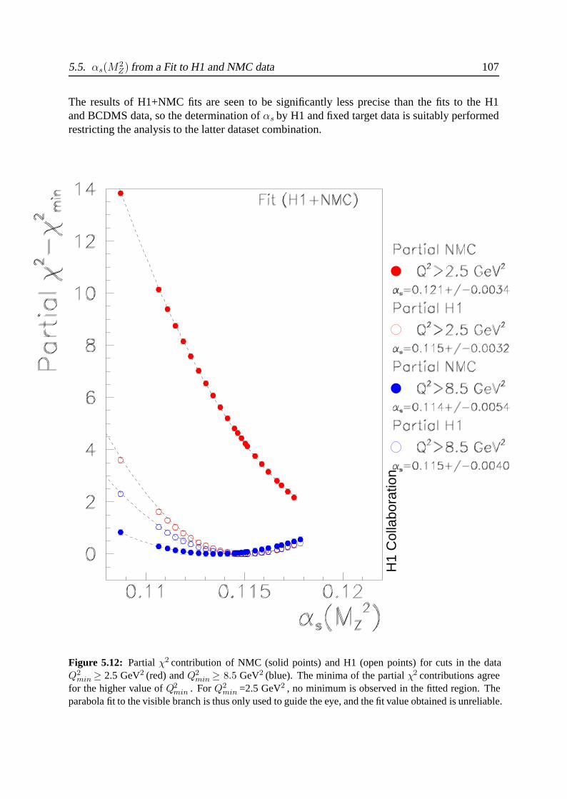
5.5. αs(M2Z) from a Fit to H1 and NMC data 107
The results of H1+NMC fits are seen to be significantly less precise than the fits to the H1and BCDMS data, so the determination of αs by H1 and fixed target data is suitably performedrestricting the analysis to the latter dataset combination.
H1
Col
labo
ratio
n
Figure 5.12: Partial χ2 contribution of NMC (solid points) and H1 (open points) for cuts in the dataQ2
min ≥ 2.5 GeV2 (red) and Q2min ≥ 8.5 GeV2 (blue). The minima of the partial χ2 contributions agree
for the higher value of Q2min . For Q2
min =2.5 GeV2 , no minimum is observed in the fitted region. Theparabola fit to the visible branch is thus only used to guide the eye, and the fit value obtained is unreliable.
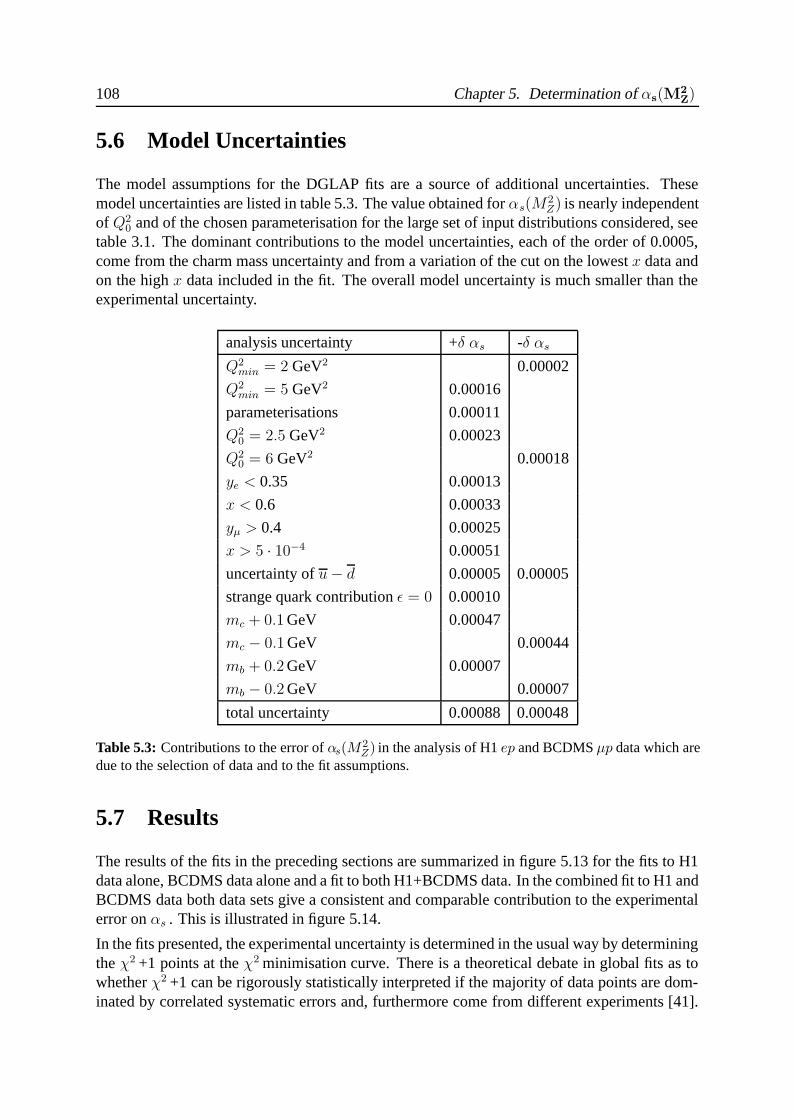
108 Chapter 5. Determination of αs(M2Z)
5.6 Model Uncertainties
The model assumptions for the DGLAP fits are a source of additional uncertainties. Thesemodel uncertainties are listed in table 5.3. The value obtained for αs(M
2Z) is nearly independent
of Q20 and of the chosen parameterisation for the large set of input distributions considered, see
table 3.1. The dominant contributions to the model uncertainties, each of the order of 0.0005,come from the charm mass uncertainty and from a variation of the cut on the lowest x data andon the high x data included in the fit. The overall model uncertainty is much smaller than theexperimental uncertainty.
analysis uncertainty +δ αs -δ αs
Q2min = 2 GeV2 0.00002
Q2min = 5 GeV2 0.00016
parameterisations 0.00011
Q20 = 2.5 GeV2 0.00023
Q20 = 6 GeV2 0.00018
ye < 0.35 0.00013
x < 0.6 0.00033
yμ > 0.4 0.00025
x > 5 · 10−4 0.00051
uncertainty of u − d 0.00005 0.00005
strange quark contribution ε = 0 0.00010
mc + 0.1 GeV 0.00047
mc − 0.1 GeV 0.00044
mb + 0.2 GeV 0.00007
mb − 0.2 GeV 0.00007
total uncertainty 0.00088 0.00048
Table 5.3: Contributions to the error of αs(M2Z) in the analysis of H1 ep and BCDMS μp data which are
due to the selection of data and to the fit assumptions.
5.7 Results
The results of the fits in the preceding sections are summarized in figure 5.13 for the fits to H1data alone, BCDMS data alone and a fit to both H1+BCDMS data. In the combined fit to H1 andBCDMS data both data sets give a consistent and comparable contribution to the experimentalerror on αs . This is illustrated in figure 5.14.
In the fits presented, the experimental uncertainty is determined in the usual way by determiningthe χ2 +1 points at the χ2 minimisation curve. There is a theoretical debate in global fits as towhether χ2 +1 can be rigorously statistically interpreted if the majority of data points are dom-inated by correlated systematic errors and, furthermore come from different experiments [41].
5.7. Results 109
In the treatment of systematic errors adopted here however the correlations are part of the min-imisation. Assuming that the correlated errors are gaussian fluctuating, χ2 retains its statisticalinterpretation [103].
The αs value thus obtained in the NLO analysis of the H1 and BCDMS proton data, applying acut yμ > 0.3, is
αs(M2Z) = 0.1150 ± 0.0017 (exp) + 0.0009
− 0.0005 (model). (5.1)
The value of this analysis of 0.1150, is lower but still consistent with the world average of0.1184 ± 0.0031 which is based on complete NNLO QCD[10]. In a moment analysis [104] ofscaling violations the effect of NNLO corrections was calculated to be
Δαs = αNLOs − αNNLO
s = 0.0012,
i.e. the value obtained in this analysis in NLO has to be compared to a world average value atNLO of αs =0.1195.
The combination of low x data with high x data determines the gluon distribution and αs . Acorrelation is observed, see figure 5.15, between αs and the parameter bg, which governs theshape of the gluon distribution at low x, see equation 3.22. Two lines are drawn which markthe behaviour of the correlation between bg and αs when αs is fixed and bg determined in the fit,solid lines, or vice versa (dashed line).
In the fit to BCDMS data alone for yμ > 0.3 and using xg = axb(1 − x)c, a χ2 minimum isfound at αs(M
2Z) = 0.111 ± 0.003 (exp) and bg is determined to be positive. A positive value
of bg implies that xg(x, Q20) falls as x decreases. The fit to BCDMS data alone thus leads to a
wrong expectation of the behaviour of xg at low x. An early αs analysis [46], in the absenceof detailed information about the low x behaviour of xg , assumed bg = 0. A positive or zerovalue of bg, for Q2
0 ≥ 4 GeV2 , is however incompatible with analyses of the HERA DIS data atlow x.
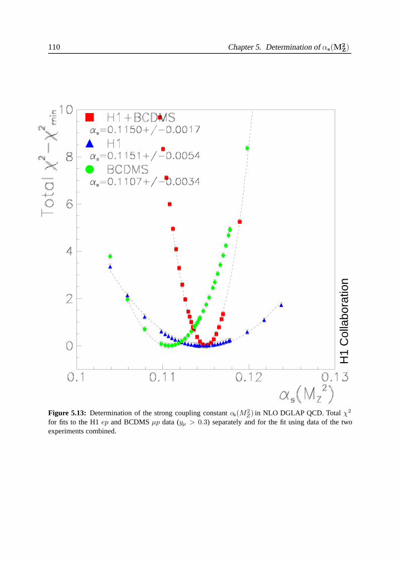
110 Chapter 5. Determination of αs(M2Z)
H1
Col
labo
ratio
n
Figure 5.13: Determination of the strong coupling constant αs(M2Z) in NLO DGLAP QCD. Total χ2
for fits to the H1 ep and BCDMS μp data (yμ > 0.3) separately and for the fit using data of the twoexperiments combined.
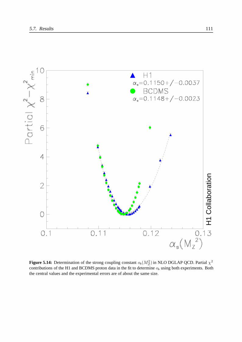
5.7. Results 111
H1
Col
labo
ratio
n
Figure 5.14: Determination of the strong coupling constant αs(M2Z) in NLO DGLAP QCD. Partial χ2
contributions of the H1 and BCDMS proton data in the fit to determine αs using both experiments. Boththe central values and the experimental errors are of about the same size.
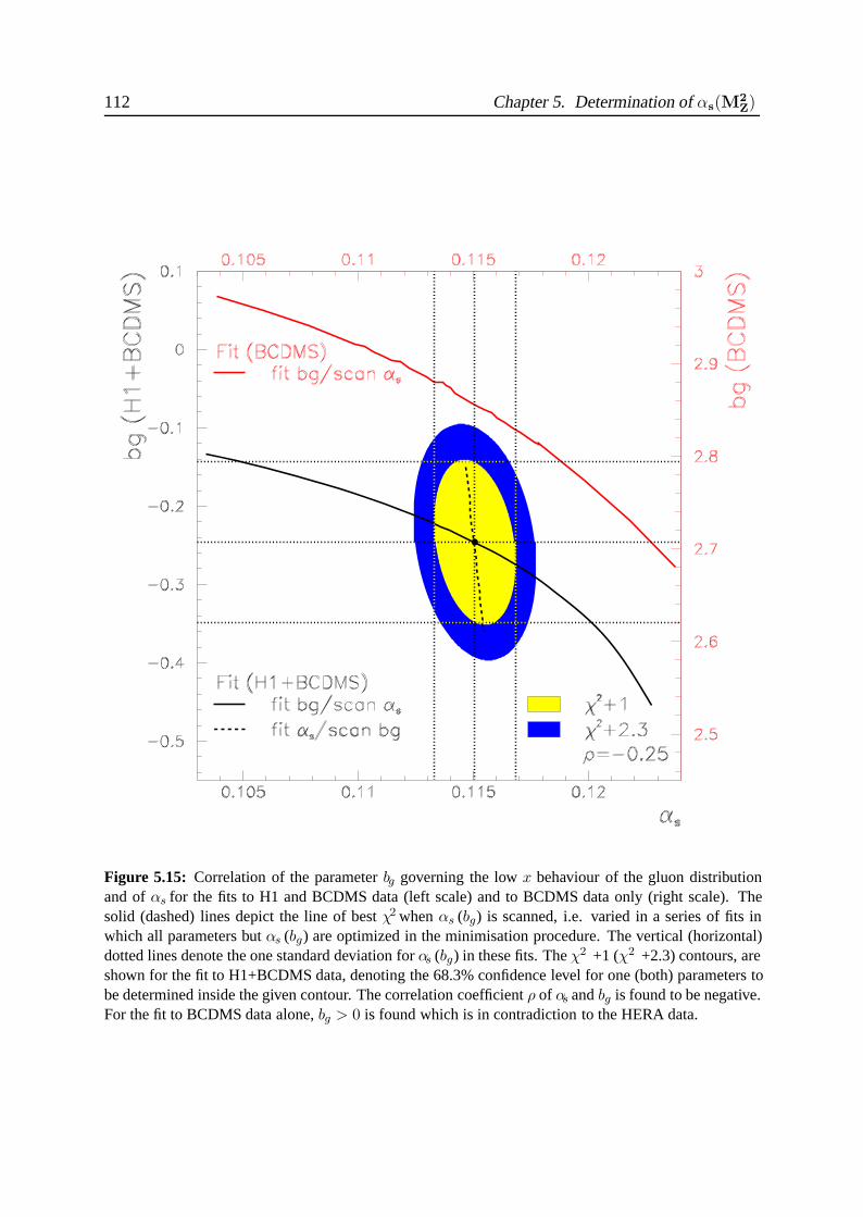
112 Chapter 5. Determination of αs(M2Z)
Figure 5.15: Correlation of the parameter bg governing the low x behaviour of the gluon distributionand of αs for the fits to H1 and BCDMS data (left scale) and to BCDMS data only (right scale). Thesolid (dashed) lines depict the line of best χ2 when αs (bg) is scanned, i.e. varied in a series of fits inwhich all parameters but αs (bg) are optimized in the minimisation procedure. The vertical (horizontal)dotted lines denote the one standard deviation for αs (bg) in these fits. The χ2 +1 (χ2 +2.3) contours, areshown for the fit to H1+BCDMS data, denoting the 68.3% confidence level for one (both) parameters tobe determined inside the given contour. The correlation coefficient ρ of αs and bg is found to be negative.For the fit to BCDMS data alone, bg > 0 is found which is in contradiction to the HERA data.
5.8. Theoretical Scale Uncertainty 113
5.8 Theoretical Scale Uncertainty
The dominant theoretical uncertainty of the NLO analysis results from the choices of the renor-malisation scale μ2
r = mr · Q2 (equation 1.13), and of the factorisation scale μ2f = mf · Q2.
In the MS renormalisation and factorisation scheme both scales are set equal to Q2, i.e. mr =mf = 1. Conventionally, the scales are varied by a factor 4 in order to quantify the effect ofthe scale uncertainties on αs . This choice is arbitrary such that the resulting error can hardlybe considered as the true error despite the fact that this convention is obeyed for comparing thesensitivity of different processes.
For the combination mr = 0.25, mf = 4, a term ∝ ln μ2r/μ
2f occurs in the splitting function
expansion with unequal factorisation and renormalisation scales
αs ·[1 + αs · β0 · ln(μ2
r/μ2f)
]P (0) + α2
s · P (1) (5.2)
leading to unphysical results [105]. This combination is thus excluded from the estimation. Theresults are summarized in table 5.4 and figure 5.16.
mr = 0.25 mr = 1 mr = 4
mf = 0.25 −0.0038 −0.0001 +0.0043
mf = 1 −0.0055 −− +0.0047
mf = 4 −− +0.0005 +0.0063
Table 5.4: Dependence of αs(M2Z) on the renormalisation and factorisation scales mf and mr, respec-
tively, expressed as the difference of αs(M2Z) obtained for scales different from one and the central value
of αs(M2Z) =0.1150. The combination mf = 4 and mr = 0.25 is abandoned since in the splitting
function expansion a term ∝ ln (mr/mf )2 becomes negative at low Q2 which causes a huge increase ofχ2.
In agreement with previous studies [49] it is found that the renormalisation scale causes a muchlarger uncertainty on αs(M
2Z) than the factorisation scale. Depending on which set of mr and
mf is chosen, the obtained χ2 differs by 5-10 units. This suggests that the assumed variation ofthe scales is indeed too large. The estimated overall uncertainty of about 0.005 on αs(M
2Z) is
much larger than the experimental error. It is expected to be significantly reduced when next-to-NLO calculations become available [19, 106]. Recently an αs analysis of moments of structurefunctions, measured in charged lepton-nucleon scattering, was presented extending to NNLOQCD [104]. The effect of the third order correction is to diminish αs(M
2Z) by about 0.001.
5.9 Further Cross Checks
The stability of the fit results is checked further with respect to possible changes in the analysisprocedure:
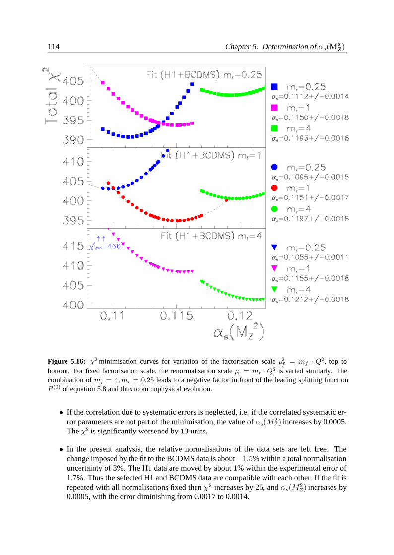
114 Chapter 5. Determination of αs(M2Z)
Figure 5.16: χ2 minimisation curves for variation of the factorisation scale μ2f = mf · Q2, top to
bottom. For fixed factorisation scale, the renormalisation scale μr = mr · Q2 is varied similarly. Thecombination of mf = 4,mr = 0.25 leads to a negative factor in front of the leading splitting functionP (0) of equation 5.8 and thus to an unphysical evolution.
• If the correlation due to systematic errors is neglected, i.e. if the correlated systematic er-ror parameters are not part of the minimisation, the value of αs(M
2Z) increases by 0.0005.
The χ2 is significantly worsened by 13 units.
• In the present analysis, the relative normalisations of the data sets are left free. Thechange imposed by the fit to the BCDMS data is about −1.5% within a total normalisationuncertainty of 3%. The H1 data are moved by about 1% within the experimental error of1.7%. Thus the selected H1 and BCDMS data are compatible with each other. If the fit isrepeated with all normalisations fixed then χ2 increases by 25, and αs(M
2Z) increases by
0.0005, with the error diminishing from 0.0017 to 0.0014.
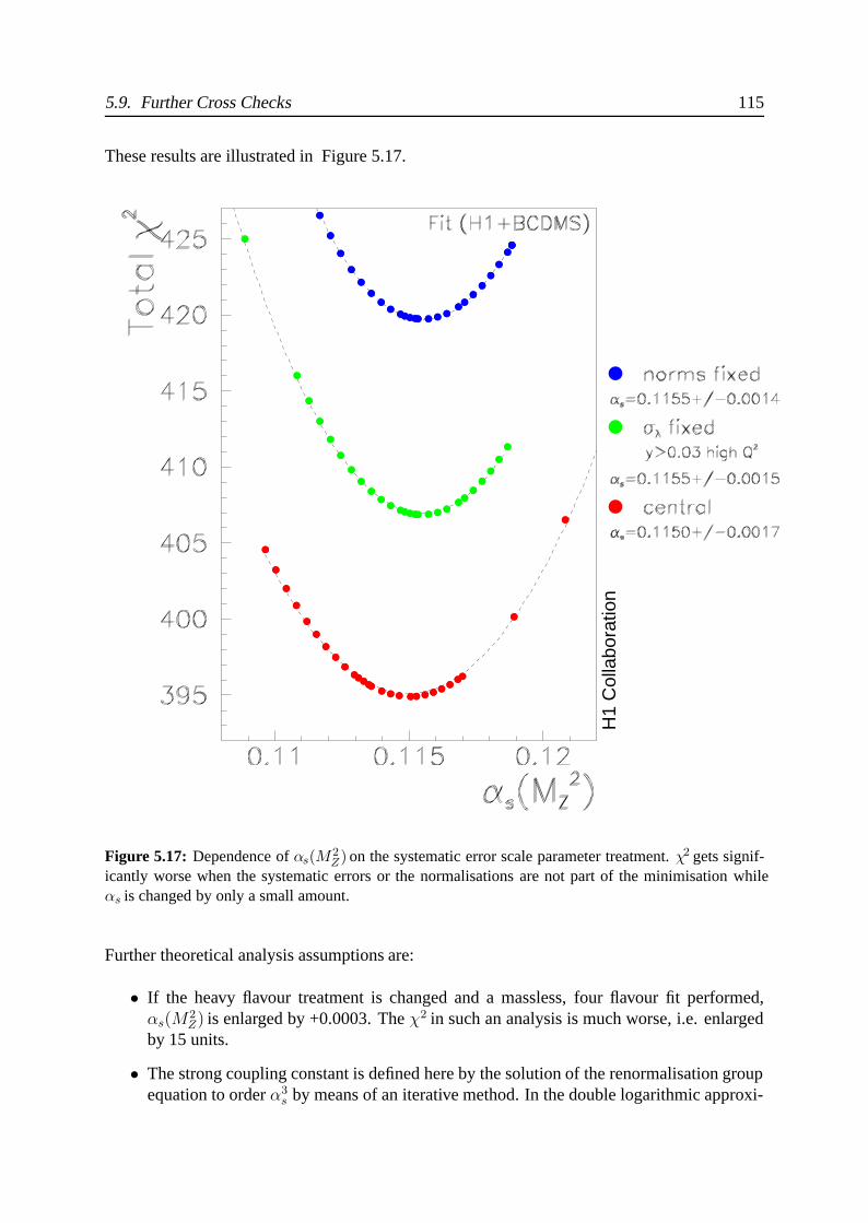
5.9. Further Cross Checks 115
These results are illustrated in Figure 5.17.
H1
Col
labo
ratio
n
Figure 5.17: Dependence of αs(M2Z) on the systematic error scale parameter treatment. χ2 gets signif-
icantly worse when the systematic errors or the normalisations are not part of the minimisation whileαs is changed by only a small amount.
Further theoretical analysis assumptions are:
• If the heavy flavour treatment is changed and a massless, four flavour fit performed,αs(M
2Z) is enlarged by +0.0003. The χ2 in such an analysis is much worse, i.e. enlarged
by 15 units.
• The strong coupling constant is defined here by the solution of the renormalisation groupequation to order α3
s by means of an iterative method. In the double logarithmic approxi-
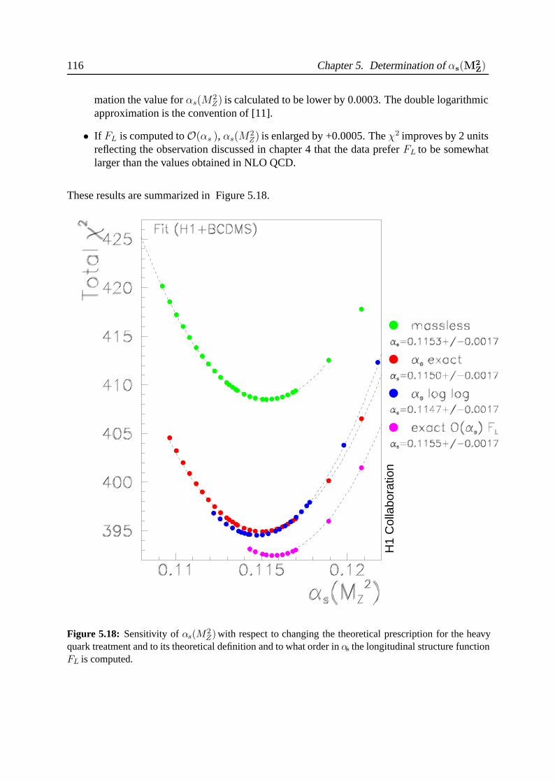
116 Chapter 5. Determination of αs(M2Z)
mation the value for αs(M2Z) is calculated to be lower by 0.0003. The double logarithmic
approximation is the convention of [11].
• If FL is computed to O(αs ), αs(M2Z) is enlarged by +0.0005. The χ2 improves by 2 units
reflecting the observation discussed in chapter 4 that the data prefer FL to be somewhatlarger than the values obtained in NLO QCD.
These results are summarized in Figure 5.18.
H1
Col
labo
ratio
n
Figure 5.18: Sensitivity of αs(M2Z) with respect to changing the theoretical prescription for the heavy
quark treatment and to its theoretical definition and to what order in αs the longitudinal structure functionFL is computed.
5.9. Further Cross Checks 117
The central result can also be compared to variations of the data sets:
• If the H1 data at high and low Q2 taken in 1996/97 are replaced by the previously pub-lished datasets taken in 1994, αs(M
2Z) comes out lower by 0.0008 with an enlarged ex-
perimental error.
• If the BCDMS data is replaced by data of the NMC collaboration [107], imposing thelow Q2 limit of the BCDMS data, a consistent value of αs(M
2Z) = 0.1158 ± 0.003 (exp)
is obtained. From the size of the experimental error it can be deduced that the NMC datamay be neglected once the BCDMS data is used.
• The addition of the BCDMS deuteron target data, with yμ > 0.3, to the H1 and BCDMSproton data yields αs(M
2Z) = 0.1158 ±0.0016 (exp), i.e. αs(M
2Z) increases by 0.0008,
while the experimental error only marginally improves. In this analysis nuclear correc-tions are applied using the integral relations of [50], and the conventional flavour decom-position into valence and sea quarks is used.
These results are summarized in Figure 5.19.
To summarise these cross checks, one observes a remarkable stability of the αs result againstquite siginficant variations in the analysis procedure and choice of datasets. The usage of H1ep and BCDMS μp provides a most accurate and clean result and remains to be preferred overanalyses which employ many datasets of hardly controllable systematic errors.
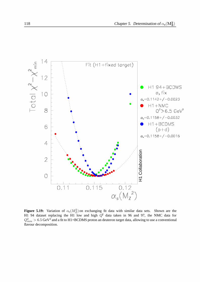
118 Chapter 5. Determination of αs(M2Z)
H1
Col
labo
ratio
n
Figure 5.19: Variation of αs(M2Z) on exchanging fit data with similar data sets. Shown are the
H1 94 dataset replacing the H1 low and high Q2 data taken in 96 and 97, the NMC data forQ2
min > 6.5 GeV2 and a fit to H1+BCDMS proton an deuteron target data, allowing to use a conventionalflavour decomposition.
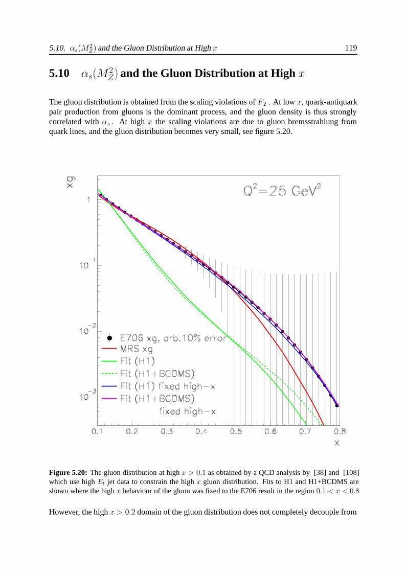
5.10. αs(M2Z) and the Gluon Distribution at High x 119
5.10 αs(M2Z) and the Gluon Distribution at High x
The gluon distribution is obtained from the scaling violations of F2 . At low x, quark-antiquarkpair production from gluons is the dominant process, and the gluon density is thus stronglycorrelated with αs . At high x the scaling violations are due to gluon bremsstrahlung fromquark lines, and the gluon distribution becomes very small, see figure 5.20.
Figure 5.20: The gluon distribution at high x > 0.1 as obtained by a QCD analysis by [38] and [108]which use high Et jet data to constrain the high x gluon distribution. Fits to H1 and H1+BCDMS areshown where the high x behaviour of the gluon was fixed to the E706 result in the region 0.1 < x < 0.8
However, the high x > 0.2 domain of the gluon distribution does not completely decouple from
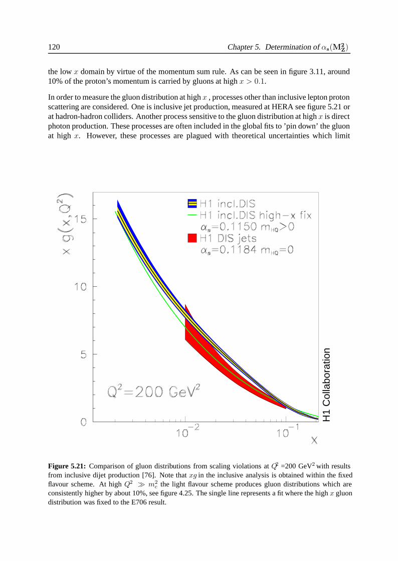
120 Chapter 5. Determination of αs(M2Z)
the low x domain by virtue of the momentum sum rule. As can be seen in figure 3.11, around10% of the proton’s momentum is carried by gluons at high x > 0.1.
In order to measure the gluon distribution at high x , processes other than inclusive lepton protonscattering are considered. One is inclusive jet production, measured at HERA see figure 5.21 orat hadron-hadron colliders. Another process sensitive to the gluon distribution at high x is directphoton production. These processes are often included in the global fits to ’pin down’ the gluonat high x. However, these processes are plagued with theoretical uncertainties which limit
H1
Col
labo
ratio
n
Figure 5.21: Comparison of gluon distributions from scaling violations at Q2 =200 GeV2 with resultsfrom inclusive dijet production [76]. Note that xg in the inclusive analysis is obtained within the fixedflavour scheme. At high Q2 � m2
c the light flavour scheme produces gluon distributions which areconsistently higher by about 10%, see figure 4.25. The single line represents a fit where the high x gluondistribution was fixed to the E706 result.
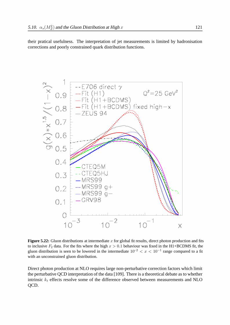
5.10. αs(M2Z) and the Gluon Distribution at High x 121
their pratical usefulness. The interpretation of jet measurements is limited by hadronisationcorrections and poorly constrained quark distribution functions.
Figure 5.22: Gluon distributions at intermediate x for global fit results, direct photon production and fitsto inclusive F2 data. For the fits where the high x > 0.1 behaviour was fixed in the H1+BCDMS fit, thegluon distribution is seen to be lowered in the intermediate 10−2 < x < 10−1 range compared to a fitwith an unconstrained gluon distribution.
Direct photon production at NLO requires large non-perturbative correction factors which limitthe perturbative QCD interpretation of the data [109]. There is a theoretical debate as to whetherintrinsic kt effects resolve some of the difference observed between measurements and NLOQCD.
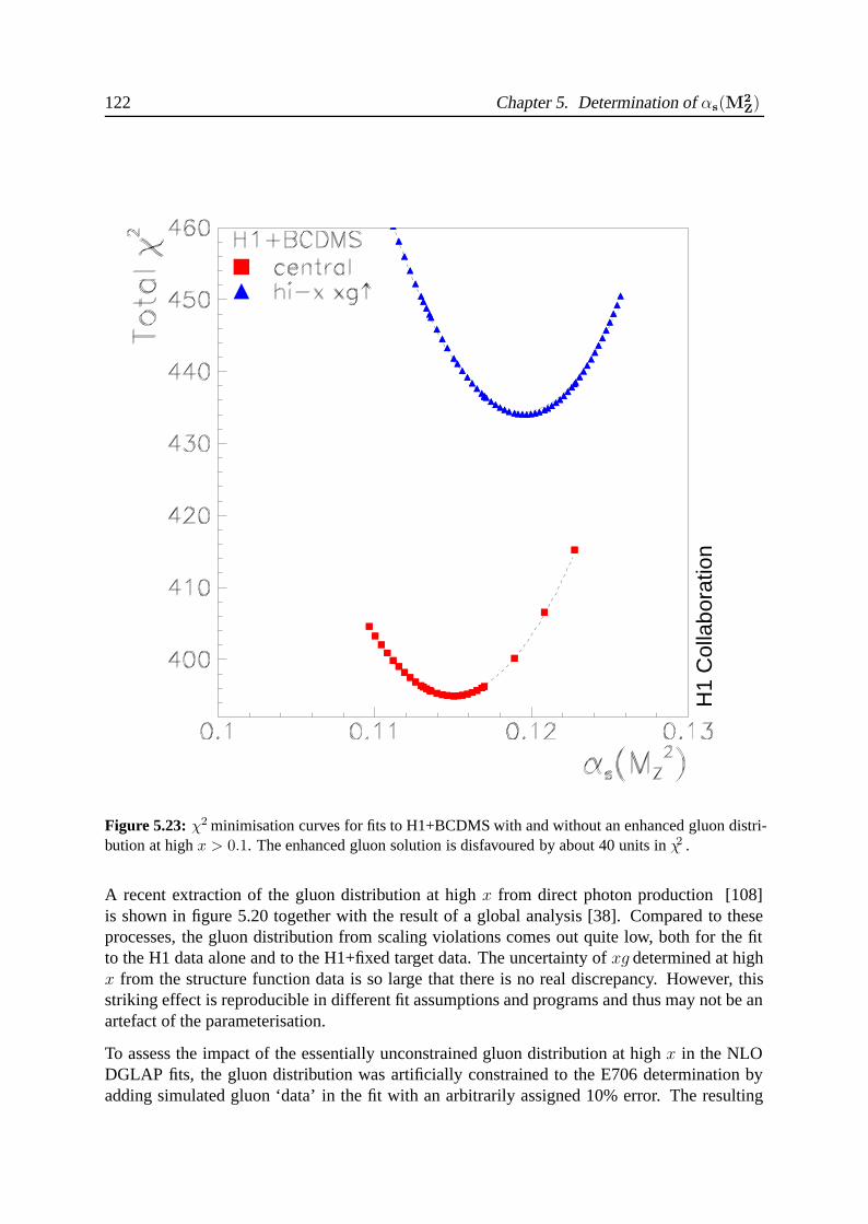
122 Chapter 5. Determination of αs(M2Z)
H1
Col
labo
ratio
n
Figure 5.23: χ2 minimisation curves for fits to H1+BCDMS with and without an enhanced gluon distri-bution at high x > 0.1. The enhanced gluon solution is disfavoured by about 40 units in χ2 .
A recent extraction of the gluon distribution at high x from direct photon production [108]is shown in figure 5.20 together with the result of a global analysis [38]. Compared to theseprocesses, the gluon distribution from scaling violations comes out quite low, both for the fitto the H1 data alone and to the H1+fixed target data. The uncertainty of xg determined at highx from the structure function data is so large that there is no real discrepancy. However, thisstriking effect is reproducible in different fit assumptions and programs and thus may not be anartefact of the parameterisation.
To assess the impact of the essentially unconstrained gluon distribution at high x in the NLODGLAP fits, the gluon distribution was artificially constrained to the E706 determination byadding simulated gluon ‘data’ in the fit with an arbitrarily assigned 10% error. The resulting
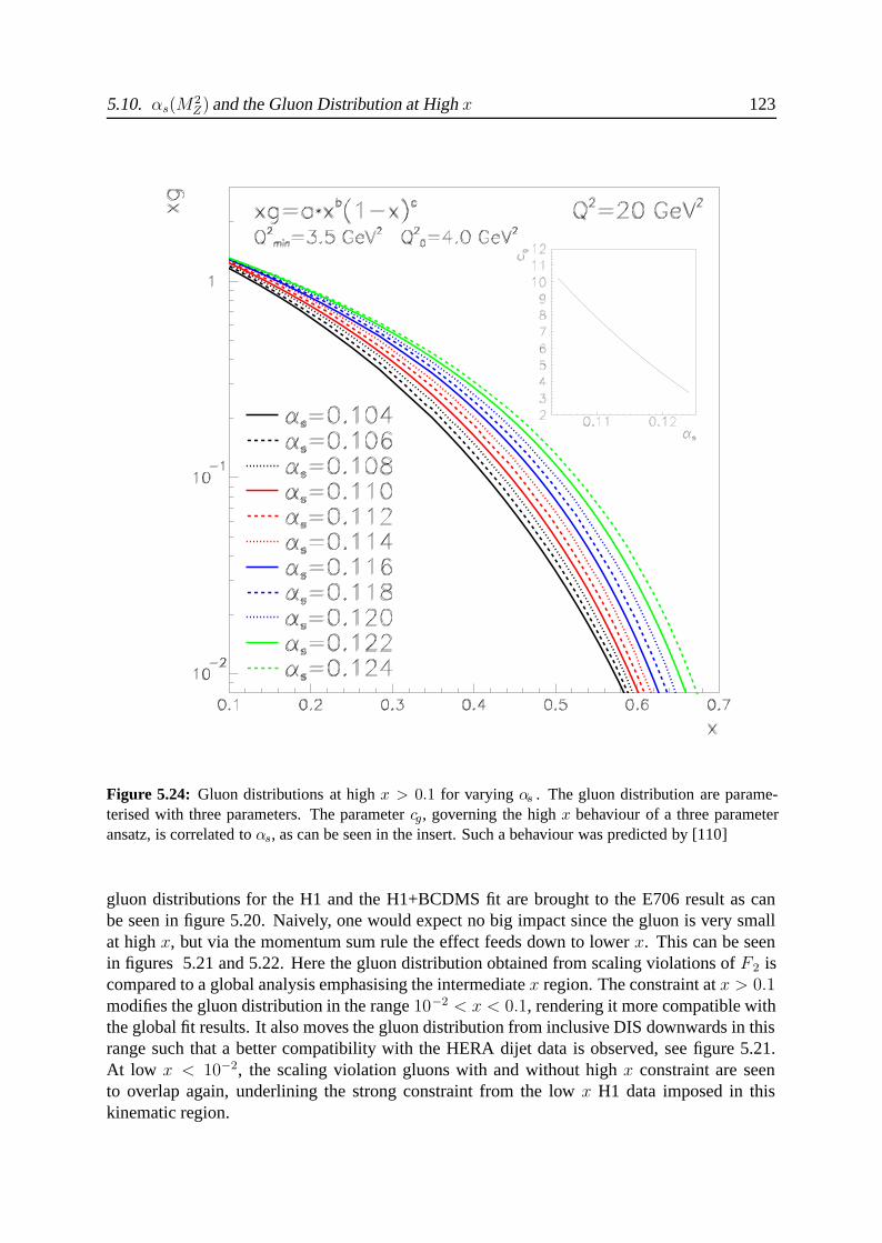
5.10. αs(M2Z) and the Gluon Distribution at High x 123
Figure 5.24: Gluon distributions at high x > 0.1 for varying αs . The gluon distribution are parame-terised with three parameters. The parameter cg, governing the high x behaviour of a three parameteransatz, is correlated to αs, as can be seen in the insert. Such a behaviour was predicted by [110]
gluon distributions for the H1 and the H1+BCDMS fit are brought to the E706 result as canbe seen in figure 5.20. Naively, one would expect no big impact since the gluon is very smallat high x, but via the momentum sum rule the effect feeds down to lower x. This can be seenin figures 5.21 and 5.22. Here the gluon distribution obtained from scaling violations of F2 iscompared to a global analysis emphasising the intermediate x region. The constraint at x > 0.1modifies the gluon distribution in the range 10−2 < x < 0.1, rendering it more compatible withthe global fit results. It also moves the gluon distribution from inclusive DIS downwards in thisrange such that a better compatibility with the HERA dijet data is observed, see figure 5.21.At low x < 10−2, the scaling violation gluons with and without high x constraint are seento overlap again, underlining the strong constraint from the low x H1 data imposed in thiskinematic region.
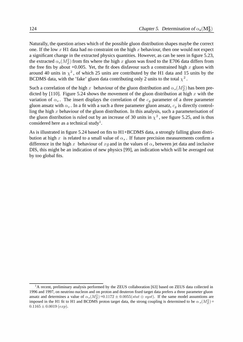
124 Chapter 5. Determination of αs(M2Z)
Naturally, the question arises which of the possible gluon distribution shapes maybe the correctone. If the low x H1 data had no constraint on the high x behaviour, then one would not expecta significant change in the extracted physics quantities. However, as can be seen in figure 5.23,the extracted αs(M
2Z) from fits where the high x gluon was fixed to the E706 data differs from
the free fits by about +0.005. Yet, the fit does disfavour such a constrained high x gluon witharound 40 units in χ2 , of which 25 units are contributed by the H1 data and 15 units by theBCDMS data, with the ’fake’ gluon data contributing only 2 units to the total χ2 .
Such a correlation of the high x behaviour of the gluon distribution and αs(M2Z) has been pre-
dicted by [110]. Figure 5.24 shows the movement of the gluon distribution at high x with thevariation of αs . The insert displays the correlation of the cg parameter of a three parametergluon ansatz with αs . In a fit with a such a three parameter gluon ansatz, cg is directly control-ling the high x behaviour of the gluon distribution. In this analysis, such a parameterisation ofthe gluon distribution is ruled out by an increase of 30 units in χ2 , see figure 5.25, and is thusconsidered here as a technical study1.
As is illustrated in figure 5.24 based on fits to H1+BCDMS data, a strongly falling gluon distri-bution at high x is related to a small value of αs . If future precision measurements confirm adifference in the high x behaviour of xg and in the values of αs between jet data and inclusiveDIS, this might be an indication of new physics [99], an indication which will be averaged outby too global fits.
1A recent, preliminary analysis performed by the ZEUS collaboration [63] based on ZEUS data collected in1996 and 1997, on neutrino nucleon and on proton and deuteron fixed target data prefers a three parameter gluonansatz and determines a value of αs(M2
Z) =0.1172 ± 0.0055(stat ⊕ syst). If the same model assumtions areimposed in the H1 fit to H1 and BCDMS proton target data, the strong coupling is determined to be α s(M2
Z) =0.1165± 0.0019 (exp).
5.10. αs(M2Z) and the Gluon Distribution at High x 125
H1
Col
labo
ratio
n
Figure 5.25: χ2 minimisation curves for a three parameter gluon distribution and a 5 parameter ansatzas used for the analyses to H1 and BCDMS data.
Summary
Deep inelastic scattering has been the most suitable process to test the theory of the stronginteraction. By means of a well defined eletroweak probe, quark-gluon interactions can bestudied in a kinematic regime where QCD is asymptotically free and allows calculations tohigher order pertubation theory.
This work discussed the so far most precise measurement of the DIS scattering cross section inthe kinematic range of low x accessed by the HERA accelerator. The low x region is accessedat lower Q2 between 1 and 150 GeV2 where the secondary positron is scattered in the backwardH1 apparatus, notably the SPACAL calorimeter and the preceding track devices, the BDC andthe BST.
With the upgraded H1 backward apparatus and a luminosity of about 20 pb−1 the inclusive DISscattering cross section was measured with typically 3% precision using data taken in 1996and 1997. Part of the published data was provided by the author and a complete analysis wasperformed for cross checks.
The high accuracy of the data allowed a precision QCD analysis to be performed with the goalsto
• verify the validity of the description of the measurement within the conventional pertur-bative QCD approach, the DGLAP equations;
• measure the gluon momentum distribution xg(x, Q2) in the proton;
• determine the strong coupling constant αs.
In a novel approach this analysis was performed using proton target data alone.
• No departure was observed of the measured cross section from the QCD calculation,which, however, requires initial parton distributions to be fixed by the data. The QCDcalculations, fixed by the scaling violations of F2 , allow accurate predictions to be madefor the longitudinal structure function FL and for the charm structure function F cc
2 whichin further analyses by H1 are shown to be well described.
• The gluon distribution xg(x, Q2) is determined at Q2 = 20 GeV2 to an experimental ac-curacy of about 3% in the kinematic range 3 · 10−4 ≤ x ≤ 0.1. The gluon density risestowards low x and no sign for saturation is observed in the DIS region.
126
5.10. αs(M2Z) and the Gluon Distribution at High x 127
• Based on on the H1 ep and the BCDMS μp data the strong coupling constant is deter-mined to NLO in the MS renormalisation and factorisation scheme:
αNLO,MSs (M2
Z) = 0.1150 ± 0.0017 (exp) + 0.0009− 0.0005 (model)
The result is consistent with the world average value but tends to be lower and has anexperimental and model uncertainty of size comparable to the average of all previousdata on αs(M
2Z) .
• The largest uncertainty of the order of ±0.005 is connected with the uncertainty of therenormalisation scale which requires this data to be re-analysed when the exact NNLOformulae become available.
This result was cross checked with quite a number of analyses using different data sets andvarying nearly all assumptions in the fit. For example, a conventional analysis using the standardflavour decomposition and deuteron data leads to a value of 0.1158 ± 0.0016 (exp).
Interesting observations were made on the correlation of αs with the behaviour of the gluondistribution both at low x and at high x. These deserve further attention when still improvedHERA data become available, in particular at high x.
“... und ging nicht alles aus, so ging doch wenigstens was vor.” (P. Hacks)
Bibliography
[1] M. Bloom et al., M. Breidenbach et al., Phys. Rev. Lett. 23 (1969) 935.
[2] R.Frisch, O. Stern, Z. Physik 85 (1933) 4.
[3] R. Hofstadter, Rev. Mod. Phys. 28 (1956) 214.
[4] R.P. Feynman, Phys. Rev. Lett. 23 (1969) 1415.
[5] M. Gell-Mann, Phys. Lett. 8 (1964), 214.
[6] C. Zweig, CERN Report Nos. TH 401,402 (1964).
[7] C.G. Callan, D.J. Gross, Phys. Rev. Lett. 22 (1969) 156.
[8] D.J. Fox et al., Phys. Rev. Lett. 33 (1974) 1504.
[9] BEBC Collaboration, Nucl. Phys. B 203 (1982) 362.
[10] S.Bethke, hep-ph/0004021 (2000).
[11] Particle Data Group Report, D.E. Groom et al., Eur. Phys. J. C 15 (2000) 1.
[12] J.C. Collins, D.E. Soper, Ann. Rev. Nucl. Part. Sci. 37 (1978) 383.
[13] W. Furmanski and R. Petronzio, Z. Physik C 11 (1982) 293.
[14] W. J. Marciano Phys. Rev. D 29 (1984) 580.
[15] G.’t Hooft, M.Veltman, Nucl. Phys. B 44 (1972) 189.
[16] G. Altarelli and G. Martinelli, Phys. Lett. B 76 (1978) 89;M. Gluck and E. Reya, Nucl. Phys. B 145 (1978) 24.
[17] E. B. Zijlstra and W. van Neerven, Nucl. Phys. B 383 (1992) 525.
[18] Yu. L. Dokshitzer, Sov. Phys. JETP 46 (1977) 641;V. N. Gribov and L. N. Lipatov, Sov. J. Nucl. Phys. 15 (1972) 438 and 675;G. Altarelli and G. Parisi, Nucl. Phys. B 126 (1977) 298.
[19] W.L. van Neerven and A. Vogt, Nucl. Phys. B 588 (2000) 345.
128
BIBLIOGRAPHY 129
[20] F. Lehner, Ph.D. Thesis, University of Hamburg (1998).
[21] H1 Collaboration, I. Abt et al., Nucl. Instrum. Meth. A386 (1997) 310 and 348.
[22] M. Klein, On the Q2, x Range at HERA, Proceedings of the Workshop Physics at HERA,vol. 1, eds. W. Buchmuller, G.Ingelman, DESY (1992).
[23] A. Blondel and F. Jacquet, Proc. ep Facility for Europe, Amsterdam 1979, DESY 79/48(1979) 391.
[24] U. Bassler and G. Bernardi, Nucl. Instrum. Meth. A361 (1995) 197.
[25] S. Bentvelsen, J. Engelen and P. Kooijman, Proc. Workshop on HERA Physics, Vol 1, eds.W. Buchmuller and G. Ingelman, Hamburg, DESY (1992) 25;K. C. Hoger, ibid 43.
[26] D. Eckstein, Ph.D. Thesis, Humboldt-University Berlin (2001).
[27] H1 Collaboration, C. Adloff et al., Eur. Phys. J. C 21 (2001) 33-61, DESY-00-181, hep-ex/0012053.
[28] E. Tzamariudaki, Proceedings of VII calorimeter conference CALOR 97, World Scientific(1998).
[29] R.Wallny, Diploma Thesis, University Heidelberg (1996).
[30] A. Meyer, Ph.D. Thesis, University of Hamburg (1997).
[31] A. A. Glazov, Ph.D. Thesis, Humboldt-University Berlin (1998).
[32] R.Stamen, Diploma Thesis, University of Dortmund (1998).
[33] R.Maracek, Ph.D. Thesis, Inst. of Exp. Physics Kosice (1999).
[34] P. Sievers, Diploma Thesis, University Heidelberg (1999).
[35] R. Engel and J. Ranft, Phys. Rev. D 54 (1996) 4244.
[36] V.V. Arkadov, Ph.D. Thesis, Humboldt-University Berlin (2000).
[37] H1 Collaboration, C. Adloff et al., Eur. Phys. J. C 13 (2000) 609.
[38] A.D. Martin et al., Eur. Phys. J. C 4 (1998) 463.
[39] CTEQ Collaboration, H.L. Lai et al., Phys. Rev. D 55 (1997) 1280 and hep-ph/9903282(1999).
[40] M. Gluck, E.Reya and A.Vogt, Eur. Phys. J. C 5 (1998) 461.
[41] W. T. Giele, S. A. Keller and D. A. Kosower, hep-ph/0104052 (2001).
[42] J. Pumplin et al., hep-ph/0101032 (2001).
130 BIBLIOGRAPHY
[43] D. Stump et al., hep-ph/0101051 (2001).
[44] A.J. Buras, Rev. Mod. Phys. 52 (1980) 199.
[45] NMC Collaboration, M. Arneodo et al., Phys. Rev. B 309 (1993) 222.
[46] A. Milsztaijn and M. Virchaux, Phys. Lett. B 274 (1992) 221.
[47] M. Botje, QCDNUM, ZEUS internal notes 98-062 (1998) and 99-027 (1999);Phys. Lett. B 472 (2000) 175.
[48] A. Alekhin, IHEP-2000-39 and hep-ph/0011002 (2000).
[49] A. Vogt, Proc. DIS’99, Nucl. Phys. B79 Proc. Suppl. (1999) 102, ed. by J. Blumlein andT. Riemann.
[50] Melnitchouk and A.W. Thomas, Phys. Rev. C 52 (1995) 3373.
[51] L.Frankfurt, M.Strikman, Eur. Phys. J. A 5 (1999) 293-306.
[52] E. Laenen et al., Nucl. Phys. B 392 (1993) 162;S. Riemersma, J. Smith and W. van Neerven, Phys. Lett. B 347 (1995) 143.
[53] CCFR Collaboration, A.O. Bazarko et al., Z. Physik C 65 (1995) 189.
[54] E866/NuSea Collaboration, E.A. Hawker et al., Phys. Rev. Lett. 80 (1998) 3715.
[55] NMC Collaboration, P. Amaudruz et al., Phys. Rev. Lett. 66 (1991) 2712 and M. Arneodoet al., Phys. Rev. D 50 (1994) R1.
[56] NuTeV Collaboration, T. Adams et al., hep-ex/9906038 (1999).
[57] R.D. Ball and S. Forte, Phys. Lett. B 335 (1994) 77-86, and Phys. Lett. B 336 (1994)77-79.
[58] A.D. Martin, Proc. of XXI International Meeting on Fundamental Physics, World Scien-tific (1993).
[59] V.Lemaitre, Proc. HEP97, Jerusalem, Israel (1997).
[60] ZEUS Collaboration , J. Breitweg et al., Eur. Phys. J. C 7 (1999) 609-630.
[61] M. Gluck, E. Reya, Phys. Lett. B 83 (1979) 9.
[62] M. Gluck, E. Reya, A. Vogt, Z. Physik C 53 (1992) 127.
[63] K.Nagano, Proc. DIS2001, Bologna, Italy (2000).
[64] CTEQ Collaboration, H.L. Lai et al., Eur. Phys. J. C 12 (2000) 375-392.
[65] CTEQ Collaboration, H.L. Lai et al., Phys. Rev. D 55 (1997) 1280.
[66] C. Pascaud and F. Zomer, LAL preprint, LAL/95-05 (1995).
BIBLIOGRAPHY 131
[67] R.J.Barlow, Statistics, John Wiley & Sons (1989).
[68] F.James, MINUIT, CERN Program Library Long Writeup D506.
[69] C. Pascaud and F. Zomer, QCDFIT manual, unpublished.
[70] K. Prytz, Phys. Lett. B 311 (1993) 286.
[71] A. Dubak, Proc. DIS2001, Bologna, Italy (2001).
[72] S.J. Brodsky and G. Farrar, Phys. Rev. Lett. 31 (1973) 1153.
[73] M. Klein, P. Newman, R. Wallny, H1-Internal Note h1-0600-585.
[74] R.Roberts, Proc. DIS2000, Liverpool, United Kingdom (2000).
[75] H1 Collaboration, I. Abt et al., Nucl. Phys. B 545 (1999) 21.
[76] H1 Collaboration, C. Adloff et al., Eur. Phys. J. C 19 (2001) 289-311.
[77] R. Thorne, R.G. Roberts Eur. Phys. J. C 19 (2001) 339-349.
[78] E.Witten, Nucl. Phys. B 104 (1996) 445.
[79] M. Shifman et al., Nucl. Phys. B 136 (1978) 157.
[80] H1 Collaboration, C. Adloff et al., submitted to Phys. Lett.B, DESY-01-100, hep-ex/0108039 (2001).
[81] ZEUS Collaboration, J. Breitweg et al., Eur. Phys. J. C 12 (2000) 35-52.
[82] D. Muller, Ph. D. Thesis, University of Zurich (1998).
[83] M. Nedden, Ph. D. Thesis, University of Zurich (1998).
[84] H1 Collaboration, C. Adloff et al., Nucl. Phys. B 545 (1999) 21-44.
[85] E. Laenen, S. Riemersma, J. Smith, W. van Neerven Nucl. Phys. B 392 (1993) 162 and229.
[86] B. Harris and J. Smith, Nucl. Phys. B 452 (1995) 109.
[87] S. Riemersma, Nucl. Phys. B 392 (1993) 162.
[88] W. L. van Neerven, Acta Phys. Polon. B28(1997) 2715.
[89] A. Vogt Proc. DIS’96 (1996).
[90] M. Aivazis, J. Collins, F. Olness, W. Tung, Phys. Rev. D 50 (1994) 3102.
[91] M. Buza et al. Eur. Phys. J. C 1 (1998) 301-320, hep-ph/9612398 (1996).
[92] A.D. Martin et al., Eur. Phys. J. C 4 (1998) 463 and hep-ph/9907231 1999.
132 BIBLIOGRAPHY
[93] T. Hadig, Ph.D. Thesis, RWTH Aachen, preprint PITHA 99/41 (1999).The program is based on J. Blumlein and A. Vogt, Phys. Rev. D 58 (1998) 014020.
[94] M. Cooper-Sarkar et al. Proc. Workshop on HERA Physics, Vol 1, ed. R.Peccei,Hamburg,DESY (1987) 231.
[95] L.A.T. Bauerdick, A.Glazov, M.Klein, Workshop on Future Physics at HERA, Hamburg,DESY (1996) 77.
[96] L.Favart et al., DESY grey report FH1K-96-01 (1996).
[97] BCDMS Collaboration, A.C. Benvenuti et al., Phys. Lett. B B223 (1989) 485;CERN preprint CERN-EP/89-06.
[98] L. Clavelli, hep-ph/9908342 (1999).
[99] J. Blumlein and J. Botts, Phys. Lett. B 325 (1994) 190; [Erratum-ibid. B331 (1994) 450]hep-ph/9401291.
[100] L. W. Whitlow et al., Phys. Lett. B 282 (1992) 475.
[101] A. Milsztaijn et al., Z. Physik C 49 (1991) 527.
[102] J. Bartels, K. Charchula and J. Feltesse, Proc. Workshop on HERA Physics, Vol 1, eds.W. Buchmuller and G. Ingelman, Hamburg, DESY (1992) 193.
[103] C. Pascaud and F. Zomer, DESY 96-266 (1996).
[104] J. Santiago and F.J. Yndurain, Nucl. Phys. B 563 (1999) 45 and Nucl. Phys. Proc. Suppl.86 (2000) 69.
[105] C.Pascaud, private communication.
[106] A. Vogt, private communication.
[107] NMC Collaboration, M. Arneodo et al., Phys. Lett. B 309 (1993) 222.
[108] E706 Collaboration, L. Apanasevich et al., Phys. Rev. Lett. 81 (1998) 2642-2645.
[109] P. Aurenche et al., Eur. Phys. J. C 39 (1999) 107-119.
[110] ’Georgi Plot’ M.Klein, private communication.

Acknowledgments
I wish to express my sincere gratitude to Prof. Ulrich Straumann for offering me the opportunityto work as a Ph.D. student for the H1 experiment. He gave me a large degree of freedom andtrust while I was pursuing my scientific goals. I thank him for his support and patience.
Heartfelt thanks go to Max Klein who has been the driving force behind this work. Maybe toodriving at times, he shared all the ups and downs of this work, and without him this analysiscertainly would not have succeeded. I could always count on his advice and continuous support,including the difficult last months of writing up this work. I much appreciated his good senseof humour and our discussions on topics outside physics as well.I also wish to thank Christian Pascaud, who provided and maintained the QCD evolution pro-gram, and who also was a steady stronghold of knowledge and advice even in Le Bourge. Itwas a distinct pleasure to see, with these two gentlemen, the first inclusive measurement of αs
from HERA emerge from the countless numbers and plots.
I also wish to express my gratitude to Doris Eckstein, Sasha Glazov, Thorsten Kleinwort, FrankLehner and Fabian Zomer. Doris and I survived the data analysis together and cheered eachother’s spirit up at the Zeuthen lake and elsewhere. Thorsten did an extremely fine job in main-taining the Linux cluster which we tortured with countless analysis and QCD fit jobs. Sashaopenly shared his wisdom concerning data analysis with me and Fabian and Frank providedtheir knowledge concerning QCD fitting for which I am very grateful.
I am indebted to my ELAN colleagues Vladimir Arkadov, Andreas Meyer, Philipp Sievers,Vladimir Shekelyan, and Sasha Zhokin. Their knowledge and co-operation in the data analysisis, albeit not documented in this thesis, distinctly felt throughout my time as a Ph.D. studentand hereby acknowledged. I also would like to thank Andreas Vogt whose help in computingthe renormalisation and factorisation scale uncertainities was much appreciated.
Much of this work has already found its way to the conferences during the spokesmanship ofProf. John Dainton. I hope he did not take it as a hideous attack on his good health whenwe shipped the preliminary data to the Stanford Lepton-Photon Conference 1999 the way wedid. Many thanks are also due to his successor Eckhard Elsen who continued supporting andencouraging this analysis.
The hospitality of the DESY Directorate (Hamburg and Zeuthen) is gratefully acknowledged,as is the hospitality of quite a different kind of David Muller und Renate Nussberger in Zurich.Frank Lehner and Phil Geissbuehler went through the pain of proof-reading on short notice, forwhich I owe them a lot. I extend my gratitude to all the colleagues at Heidelberg, Hamburg,Zurich and Zeuthen; physicists, engineers and technicians, who are too numerous to mentionbut enriched my life while I was in their midst. Thank you all.
The last words of gratitude belong to my family, especially to my mother. Her example ofbearing adversity with perseverance spurred me to prove that we are akin indeed.
This work has been supported by the German Bundesministerium fur Bildung und Forschungand the Swiss National Science Foundation.
Curriculum VitaePersonalien:
Name: Rainer WallnyStaatsangehorigkeit: deutschGeboren: 12.August 1969 in Esslingen am Neckar, Deutschland
Bildungsgang:
1976 - 1980 Grundschule in Reutlingen Rommelsbach1980 - 1989 Albert-Einstein-Gymnasium Reutlingen1989 Abitur1989 - 1992 Studium der Physik an der Universitat Tubingen1991 Vordiplom1992 - 1994 Studium der Physik an der University of Washington, Seattle, WA, U.S.A.1994 Master of Science Abschluss1994 - 1996 Studium der Physik an der Universitat Heidelberg1995 - 1996 Diplomarbeit in Experimentalphysik unter der Leitung
von Prof. Dr. U. Straumann1996 Diplom in Experimentalphysik1995 - 1997 Forschungsaufenthalt DESY Hamburg1997 - 1999 Wissenschaftliche Mitarbeit beim H1 Experiment am
Physikalischen Institut der Universitat Heidelberg,1997 - 2000 Forschungsaufenthalt DESY Zeuthen1999 - 2001 Wissenschaftliche Mitarbeit beim H1 Experiment am
Physikinstitut der Universitat Zurich,Dissertation bei Prof. Dr. U. Straumann.
Dozentenverzeichnis:Universitat Zurich:
U. Straumann P. Truol
Universitat Heidelberg:
H.-G.Bock F.Eisele D.Habs W.Hoffmann S.HunklingerE.-E.Kluge K.T.Knopfle J.v.Krogh K-.H.Meyer H.-W.SiebertI.Stamatescu K.Tittel H.-A.Weidenmuller F.Wegner
University of Washington:
D.G.Boulware L.S.Brown V. Chaloupka S.D.Ellis L.G.JaffeG.A.Miller P.C.Peters J.E.Rothberg S.R.Sharpe

135
Universitat Tubingen:
M.Baumann A.Fassler H.Fischer F.Gonnenwein W.-D. HartmannR.Hubener H.Kaul B.Kummerer F.Lenz E.LindnerH.Muther H.Pfister H.Reinhard H.Ruder A.SchwenkG.Staudt G.Wagner