A Mathematical Introduction to Traffic Flow Theory -...
69
A Mathematical Introduction to Traffic Flow Theory Benjamin Seibold (Temple University) 0 1 2 3 density ρ Flow rate Q (veh/sec) 0 ρ max Flow rate curve for LWR model sensor data flow rate function Q(ρ) September 9–11, 2015 Tutorials Traffic Flow Institute for Pure and Applied Mathematics, UCLA Benjamin Seibold (Temple University) Mathematical Intro to Traffic Flow Theory 09/09–11/2015, IPAM Tutorials 1 / 69
Transcript of A Mathematical Introduction to Traffic Flow Theory -...
A Mathematical Introduction toTraffic Flow Theory
Benjamin Seibold (Temple University)
0
1
2
3
density ρ
Flo
w r
ate
Q (
veh/s
ec)
0 ρmax
Flow rate curve for LWR model
sensor data
flow rate function Q(ρ)
September 9–11, 2015
Tutorials Traffic Flow
Institute for Pure and Applied Mathematics, UCLA
Benjamin Seibold (Temple University) Mathematical Intro to Traffic Flow Theory 09/09–11/2015, IPAM Tutorials 1 / 69
References for Further Reading
Some References for Further Reading
general: wikipedia (can be used for almost every technical term)
traffic flow theory: wikibooks, “Fundamentals of Transportation/Traffic Flow”;Hall, “Traffic Stream Characteristics”; Immers, Logghe, “Traffic Flow Theory”
traffic models: review papers by Bellomo, Dogbe, Helbing
traffic phase theory: papers by Kerner, et al.
optimal velocity models and follow-the-leader models: papers by Bando,Hesebem, Nakayama, Shibata, Sugiyama, Gazis, Herman, Rothery, Helbing, et al.
connections between micro and macro models: papers by Aw, Klar, Materne,Rascle, Greenberg, et al.
first-order macroscopic models: papers by Lighthill, Whitham, Richards, et al.
second-order macroscopic models: papers by Whitham, Payne, Aw, Rascle,Zhang, Greenberg, Helbing, et al.
cellular models and cell transmission models: papers by Nagel, Schreckenberg,Daganzo, et al.
numerical methods for hyperbolic conservation laws: books by LeVeque
traffic networks: papers by Holden, Risebro, Piccoli, Herty, Klar, Rascle, et al.
Benjamin Seibold (Temple University) Mathematical Intro to Traffic Flow Theory 09/09–11/2015, IPAM Tutorials 2 / 69
References for Further Reading
Overview
1 Fundamentals of Traffic Flow Theory
2 Traffic Models — An Overview
3 The Lighthill-Whitham-Richards Model
4 Second-Order Macroscopic Models
5 Finite Volume and Cell-Transmission Models
6 Traffic Networks
7 Microscopic Traffic Models
Benjamin Seibold (Temple University) Mathematical Intro to Traffic Flow Theory 09/09–11/2015, IPAM Tutorials 3 / 69
Fundamentals of Traffic Flow Theory
Overview
1 Fundamentals of Traffic Flow Theory
2 Traffic Models — An Overview
3 The Lighthill-Whitham-Richards Model
4 Second-Order Macroscopic Models
5 Finite Volume and Cell-Transmission Models
6 Traffic Networks
7 Microscopic Traffic Models
Benjamin Seibold (Temple University) Mathematical Intro to Traffic Flow Theory 09/09–11/2015, IPAM Tutorials 4 / 69
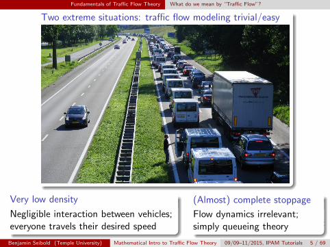
Fundamentals of Traffic Flow Theory What do we mean by “Traffic Flow”?
Two extreme situations: traffic flow modeling trivial/easy
Very low density
Negligible interaction between vehicles;everyone travels their desired speed
(Almost) complete stoppage
Flow dynamics irrelevant;simply queueing theory
Benjamin Seibold (Temple University) Mathematical Intro to Traffic Flow Theory 09/09–11/2015, IPAM Tutorials 5 / 69
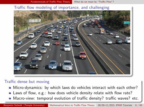
Fundamentals of Traffic Flow Theory What do we mean by “Traffic Flow”?
Traffic flow modeling of importance, and challenging
Traffic dense but moving
Micro-dynamics: by which laws do vehicles interact with each other?Laws of flow, e.g.: how does vehicle density relate with flow rate?Macro-view: temporal evolution of traffic density? traffic waves? etc.
Benjamin Seibold (Temple University) Mathematical Intro to Traffic Flow Theory 09/09–11/2015, IPAM Tutorials 6 / 69
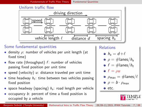
Fundamentals of Traffic Flow Theory Fundamental Quantities
Uniform traffic flow
-driving direction
vehicle length ` distance d spacing hs
-speed
Some fundamental quantities• density ρ: number of vehicles per unit length (at
fixed time)
• flow rate (throughput) f : number of vehiclespassing fixed position per unit time
• speed (velocity) u: distance traveled per unit time
• time headway ht : time between two vehicles passingfixed position
• space headway (spacing) hs : road length per vehicle
• occupancy b: percent of time a fixed position isoccupied by a vehicle
Relations
hs = d+`
ρ = #lanes/hsf = #lanes/htf = ρu
ρmax = #lanes/`
ρ = b · ρmax
etc.
Benjamin Seibold (Temple University) Mathematical Intro to Traffic Flow Theory 09/09–11/2015, IPAM Tutorials 7 / 69
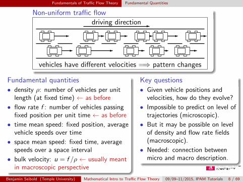
Fundamentals of Traffic Flow Theory Fundamental Quantities
Non-uniform traffic flow
- - - - -
- - - - - -
-driving direction
vehicles have different velocities =⇒ pattern changes
Fundamental quantities
• density ρ: number of vehicles per unitlength (at fixed time) ← as before
• flow rate f : number of vehicles passingfixed position per unit time ← as before
• time mean speed: fixed position, averagevehicle speeds over time
• space mean speed: fixed time, averagespeeds over a space interval
• bulk velocity: u = f /ρ ← usually meantin macroscopic perspective
Key questions
• Given vehicle positions andvelocities, how do they evolve?
• Impossible to predict on level oftrajectories (microscopic).
• But it may be possible on levelof density and flow rate fields(macroscopic).
• Needed: connection betweenmicro and macro description.
Benjamin Seibold (Temple University) Mathematical Intro to Traffic Flow Theory 09/09–11/2015, IPAM Tutorials 8 / 69

Fundamentals of Traffic Flow Theory Micro vs. Macro
Microscopic description
individual vehicletrajectories
vehicle position: xj(t)
vehicle velocity:
xj(t) =dxjdt (t)
acceleration: xj(t)
Macroscopic description
field quantities,defined everywhere
vehicle density: ρ(x , t)
velocity field: u(x , t)
flow-rate field:f (x , t) = ρ(x , t)u(x , t)
Micro view distinguishes vehicles;macro view does not.
Traffic flow has intrinsic irreproducibility.
No hope to describe/predict precise vehicle
trajectories via models [also, privacy
issues]. But, prediction of large-scale field
quantities may be possible.
Benjamin Seibold (Temple University) Mathematical Intro to Traffic Flow Theory 09/09–11/2015, IPAM Tutorials 9 / 69
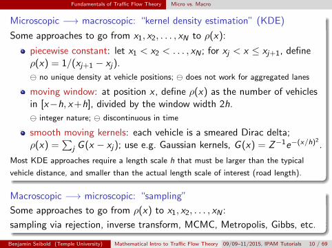
Fundamentals of Traffic Flow Theory Micro vs. Macro
Microscopic −→ macroscopic: “kernel density estimation” (KDE)
Some approaches to go from x1, x2, . . . , xN to ρ(x):
piecewise constant: let x1 < x2 < . . . , xN ; for xj < x ≤ xj+1, defineρ(x) = 1/(xj+1 − xj).
no unique density at vehicle positions; does not work for aggregated lanes
moving window: at position x , define ρ(x) as the number of vehiclesin [x−h, x+h], divided by the window width 2h.
integer nature; discontinuous in time
smooth moving kernels: each vehicle is a smeared Dirac delta;ρ(x) =
∑j G (x − xj); use e.g. Gaussian kernels, G (x) = Z−1e−(x/h)2
.
Most KDE approaches require a length scale h that must be larger than the typical
vehicle distance, and smaller than the actual length scale of interest (road length).
Macroscopic −→ microscopic: “sampling”
Some approaches to go from ρ(x) to x1, x2, . . . , xN :
sampling via rejection, inverse transform, MCMC, Metropolis, Gibbs, etc.
Benjamin Seibold (Temple University) Mathematical Intro to Traffic Flow Theory 09/09–11/2015, IPAM Tutorials 10 / 69
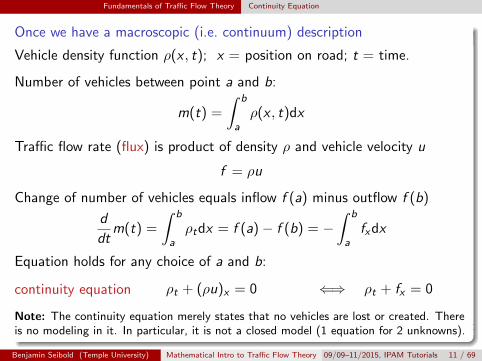
Fundamentals of Traffic Flow Theory Continuity Equation
Once we have a macroscopic (i.e. continuum) description
Vehicle density function ρ(x , t); x = position on road; t = time.
Number of vehicles between point a and b:
m(t) =
∫ b
aρ(x , t)dx
Traffic flow rate (flux) is product of density ρ and vehicle velocity u
f = ρu
Change of number of vehicles equals inflow f (a) minus outflow f (b)
d
dtm(t) =
∫ b
aρtdx = f (a)− f (b) = −
∫ b
afxdx
Equation holds for any choice of a and b:
ρt + (ρu)x = 0 ⇐⇒ ρt + fx = 0continuity equation
Note: The continuity equation merely states that no vehicles are lost or created. Thereis no modeling in it. In particular, it is not a closed model (1 equation for 2 unknowns).
Benjamin Seibold (Temple University) Mathematical Intro to Traffic Flow Theory 09/09–11/2015, IPAM Tutorials 11 / 69
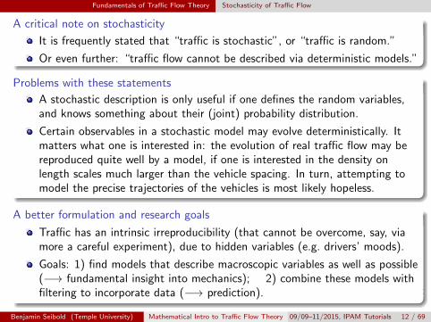
Fundamentals of Traffic Flow Theory Stochasticity of Traffic Flow
A critical note on stochasticity
It is frequently stated that “traffic is stochastic”, or “traffic is random.”
Or even further: “traffic flow cannot be described via deterministic models.”
Problems with these statements
A stochastic description is only useful if one defines the random variables,and knows something about their (joint) probability distribution.
Certain observables in a stochastic model may evolve deterministically. Itmatters what one is interested in: the evolution of real traffic flow may bereproduced quite well by a model, if one is interested in the density onlength scales much larger than the vehicle spacing. In turn, attempting tomodel the precise trajectories of the vehicles is most likely hopeless.
A better formulation and research goals
Traffic has an intrinsic irreproducibility (that cannot be overcome, say, viamore a careful experiment), due to hidden variables (e.g. drivers’ moods).
Goals: 1) find models that describe macroscopic variables as well as possible(−→ fundamental insight into mechanics); 2) combine these models withfiltering to incorporate data (−→ prediction).
Benjamin Seibold (Temple University) Mathematical Intro to Traffic Flow Theory 09/09–11/2015, IPAM Tutorials 12 / 69
Fundamentals of Traffic Flow Theory Measurements
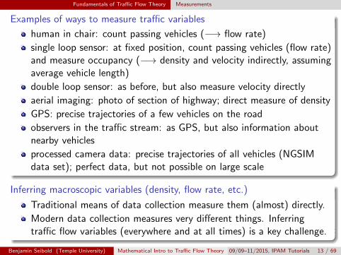
Examples of ways to measure traffic variables
human in chair: count passing vehicles (−→ flow rate)
single loop sensor: at fixed position, count passing vehicles (flow rate)and measure occupancy (−→ density and velocity indirectly, assumingaverage vehicle length)
double loop sensor: as before, but also measure velocity directly
aerial imaging: photo of section of highway; direct measure of density
GPS: precise trajectories of a few vehicles on the road
observers in the traffic stream: as GPS, but also information aboutnearby vehicles
processed camera data: precise trajectories of all vehicles (NGSIMdata set); perfect data, but not possible on large scale
Inferring macroscopic variables (density, flow rate, etc.)
Traditional means of data collection measure them (almost) directly.
Modern data collection measures very different things. Inferringtraffic flow variables (everywhere and at all times) is a key challenge.
Benjamin Seibold (Temple University) Mathematical Intro to Traffic Flow Theory 09/09–11/2015, IPAM Tutorials 13 / 69
Fundamentals of Traffic Flow Theory First Traffic Measurements and Fundamental Diagram
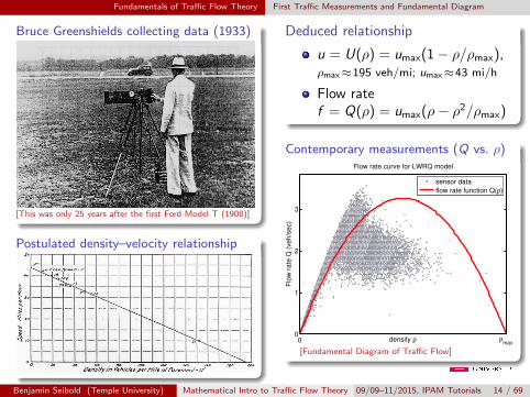
Bruce Greenshields collecting data (1933)
[This was only 25 years after the first Ford Model T (1908)]
Postulated density–velocity relationship
Deduced relationship
u = U(ρ) = umax(1− ρ/ρmax),ρmax≈195 veh/mi; umax≈43 mi/h
Flow ratef = Q(ρ) = umax(ρ− ρ2/ρmax)
Contemporary measurements (Q vs. ρ)
0
1
2
3
density ρ
Flo
w r
ate
Q (
veh/s
ec)
0 ρmax
Flow rate curve for LWRQ model
sensor data
flow rate function Q(ρ)
[Fundamental Diagram of Traffic Flow]
Benjamin Seibold (Temple University) Mathematical Intro to Traffic Flow Theory 09/09–11/2015, IPAM Tutorials 14 / 69
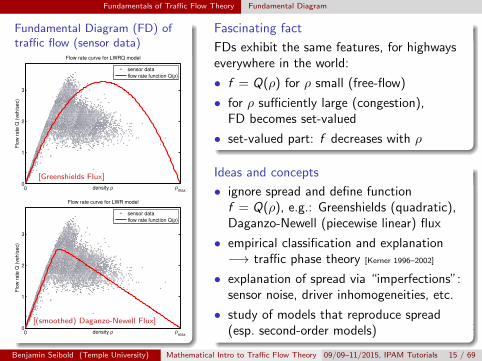
Fundamentals of Traffic Flow Theory Fundamental Diagram
Fundamental Diagram (FD) oftraffic flow (sensor data)
0
1
2
3
density ρ
Flo
w r
ate
Q (
veh/s
ec)
0 ρmax
Flow rate curve for LWRQ model
sensor data
flow rate function Q(ρ)
[Greenshields Flux]
0
1
2
3
density ρ
Flo
w r
ate
Q (
veh/s
ec)
0 ρmax
Flow rate curve for LWR model
sensor data
flow rate function Q(ρ)
[(smoothed) Daganzo-Newell Flux]
Fascinating fact
FDs exhibit the same features, for highwayseverywhere in the world:
• f = Q(ρ) for ρ small (free-flow)
• for ρ sufficiently large (congestion),FD becomes set-valued
• set-valued part: f decreases with ρ
Ideas and concepts
• ignore spread and define functionf = Q(ρ), e.g.: Greenshields (quadratic),Daganzo-Newell (piecewise linear) flux
• empirical classification and explanation−→ traffic phase theory [Kerner 1996–2002]
• explanation of spread via “imperfections”:sensor noise, driver inhomogeneities, etc.
• study of models that reproduce spread(esp. second-order models)
Benjamin Seibold (Temple University) Mathematical Intro to Traffic Flow Theory 09/09–11/2015, IPAM Tutorials 15 / 69
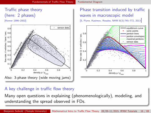
Fundamentals of Traffic Flow Theory Fundamental Diagram
Traffic phase theory(here: 2 phases)[Kerner 1996–2002]
0 0.2 0.4 0.6 0.8 10
0.1
0.2
0.3
0.4
0.5
0.6
0.7
0.8
0.9
Free
flow
cur
ve
Synchronized flow
density ρ / ρmax
flow
rat
e: #
veh
icle
s / l
ane
/ sec
.
sensor data
Also: 3-phase theory (wide moving jams)
Phase transition induced by trafficwaves in macroscopic model[S, Flynn, Kasimov, Rosales, NHM 8(3):745–772, 2013]
0 0.2 0.4 0.6 0.8 10
0.2
0.4
0.6
0.8
density ρ / ρmax
flow
rat
e Q
: # v
ehic
les
/ sec
.
equilibrium curvesonic pointsjamiton linesjamiton envelopesmaximal jamitonssensor data
A key challenge in traffic flow theory
Many open questions in explaining (phenomenologically), modeling, andunderstanding the spread observed in FDs.
Benjamin Seibold (Temple University) Mathematical Intro to Traffic Flow Theory 09/09–11/2015, IPAM Tutorials 16 / 69

Traffic Models — An Overview
Overview
1 Fundamentals of Traffic Flow Theory
2 Traffic Models — An Overview
3 The Lighthill-Whitham-Richards Model
4 Second-Order Macroscopic Models
5 Finite Volume and Cell-Transmission Models
6 Traffic Networks
7 Microscopic Traffic Models
Benjamin Seibold (Temple University) Mathematical Intro to Traffic Flow Theory 09/09–11/2015, IPAM Tutorials 17 / 69
Traffic Models — An Overview The Point of Models
One can study traffic flow empirically, i.e., observe and classify what onesees and measures.
So why study traffic models?
Can remove/add specific effects (lane switching, driver/vehicleinhomogeneities, road conditions, etc.) −→ understand which effectsplay which role.
Can study effect of model parameters (driver aggressiveness, etc.).
Can be analyzed theoretically (to a certain extent).
Can use computational resources to simulate.
Yield quantitative predictions (−→ traffic forecasting).
We actually do not really know (exactly) how we drive. Models thatproduce correct emergent phenomena help us understand our drivingbehavior.
Traffic models can be studied purely theoretically (mathematicalproperties). That is fun; but ultimately models must be validatedwith real data to investigate how well they reproduce real traffic flow.
Benjamin Seibold (Temple University) Mathematical Intro to Traffic Flow Theory 09/09–11/2015, IPAM Tutorials 18 / 69
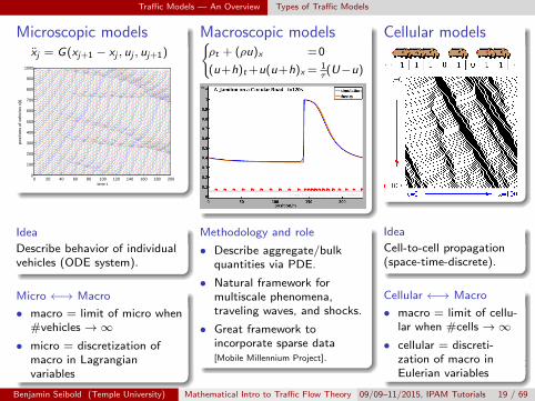
Traffic Models — An Overview Types of Traffic Models
Microscopic modelsxj = G(xj+1 − xj , uj , uj+1)
0 20 40 60 80 100 120 140 160 180 2000
100
200
300
400
500
600
700
800
900
1000
time t
posi
tions
of v
ehic
les
x(t)
Idea
Describe behavior of individualvehicles (ODE system).
Micro ←→ Macro
• macro = limit of micro when#vehicles →∞
• micro = discretization ofmacro in Lagrangianvariables
Macroscopic models{ρt + (ρu)x =0
(u+h)t +u(u+h)x = 1τ(U−u)
Methodology and role
• Describe aggregate/bulkquantities via PDE.
• Natural framework formultiscale phenomena,traveling waves, and shocks.
• Great framework toincorporate sparse data[Mobile Millennium Project].
Cellular models
Idea
Cell-to-cell propagation(space-time-discrete).
Cellular ←→ Macro
• macro = limit of cellu-lar when #cells →∞
• cellular = discreti-zation of macro inEulerian variables
Benjamin Seibold (Temple University) Mathematical Intro to Traffic Flow Theory 09/09–11/2015, IPAM Tutorials 19 / 69
Traffic Models — An Overview Microscopic Traffic Models
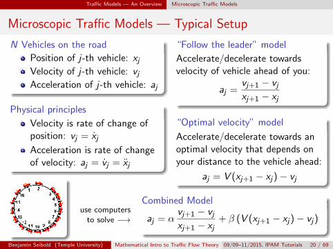
Microscopic Traffic Models — Typical Setup
N Vehicles on the road
Position of j-th vehicle: xjVelocity of j-th vehicle: vjAcceleration of j-th vehicle: aj
Physical principles
Velocity is rate of change ofposition: vj = xj
Acceleration is rate of changeof velocity: aj = vj = xj
“Follow the leader” model
Accelerate/decelerate towardsvelocity of vehicle ahead of you:
aj =vj+1 − vjxj+1 − xj
“Optimal velocity” model
Accelerate/decelerate towards anoptimal velocity that depends onyour distance to the vehicle ahead:
aj = V (xj+1 − xj)− vj
use computersto solve −→
Combined Model
aj = αvj+1 − vjxj+1 − xj
+ β (V (xj+1 − xj)− vj)
Benjamin Seibold (Temple University) Mathematical Intro to Traffic Flow Theory 09/09–11/2015, IPAM Tutorials 20 / 69
Traffic Models — An Overview Microscopic Traffic Models
Microscopic Traffic Models — Philosophy
Philosophy of microscopic models
Compute trajectories of each vehicle.
Can be extended to multiple lanes (with lane switching), differentvehicle types, etc.
At the core of most micro-simulators (e.g., Aimsun, using the Gipps’model; or Vissim, using the Wiedemann model); usually with adiscrete time-step.
Many other car-following models, e.g., the intelligent driver model.
May have many parameters, in particular free parameters that cannotbe measured directly. Hence, calibration required.
In most applications, initial positions of vehicles not known precisely.Ensembles of computations must be run.
Good for simulation (“How would a lane-closure affect this highwaysection?”); not the best framework for estimation and predictionbased on sparse/noisy data.
Benjamin Seibold (Temple University) Mathematical Intro to Traffic Flow Theory 09/09–11/2015, IPAM Tutorials 21 / 69
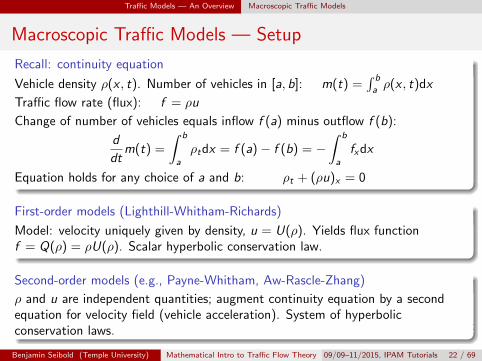
Traffic Models — An Overview Macroscopic Traffic Models
Macroscopic Traffic Models — Setup
Recall: continuity equation
Vehicle density ρ(x , t). Number of vehicles in [a, b]: m(t) =∫ b
aρ(x , t)dx
Traffic flow rate (flux): f = ρu
Change of number of vehicles equals inflow f (a) minus outflow f (b):
d
dtm(t) =
∫ b
a
ρtdx = f (a)− f (b) = −∫ b
a
fxdx
Equation holds for any choice of a and b: ρt + (ρu)x = 0
First-order models (Lighthill-Whitham-Richards)
Model: velocity uniquely given by density, u = U(ρ). Yields flux functionf = Q(ρ) = ρU(ρ). Scalar hyperbolic conservation law.
Second-order models (e.g., Payne-Whitham, Aw-Rascle-Zhang)
ρ and u are independent quantities; augment continuity equation by a secondequation for velocity field (vehicle acceleration). System of hyperbolicconservation laws.
Benjamin Seibold (Temple University) Mathematical Intro to Traffic Flow Theory 09/09–11/2015, IPAM Tutorials 22 / 69
Traffic Models — An Overview Macroscopic Traffic Models
Macroscopic Traffic Models — Philosophy
Philosophy of macroscopic models
Equations for macroscopic traffic variables.
Usually lane-aggregated, but multi-lane models can also beformulated.
Natural framework for multiscale phenomena, traveling waves, shocks.
Established theory of control and coupling conditions for networks.
Nice framework to fill gaps in incorporated measurement data.
Mathematically related with other models, e.g., microscopic models,mesoscopic (kinetic) models, cell transmission models, stochasticmodels.
Good for estimation and prediction, and for mathematical analysis ofemergent features. Not the best framework if vehicle trajectories areof interest. Also, analysis and numerical methods for PDE are morecomplicated than for ODE.
Benjamin Seibold (Temple University) Mathematical Intro to Traffic Flow Theory 09/09–11/2015, IPAM Tutorials 23 / 69
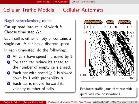
Traffic Models — An Overview Cellular Traffic Models
Cellular Traffic Models — Cellular Automata
Nagel-Schreckenberg model
Cut up road into cells of width h.Choose time step ∆t.
Each cell is either empty or contains asingle car. A car has a discrete speed.
In each time-step, do the following:
1 All cars have speed increased by 1.2 For each car reduce its speed to
the number of empty cells ahead.3 Each car with speed ≥ 2 is slowed
down by 1 with probability p.4 Each car is moved forward its
velocity number of cells. Produces traffic jams that resemble
quite well real observations.
Benjamin Seibold (Temple University) Mathematical Intro to Traffic Flow Theory 09/09–11/2015, IPAM Tutorials 24 / 69
Traffic Models — An Overview Cellular Traffic Models
Cellular Traffic Models — Cell Transmission Models
Cell Transmission Models (CTM)
Cut up road into cells of width h. Choose time step ∆t.
Each cell contains an average density ρj . In each step, a certain fluxof vehicles, fj+ 1
2, travels from cell j to cell j + 1. The fluxes between
cells change the densities in the cells accordingly.
The flux depends on the adjacent cells: fj+ 12
= F (ρj , ρj+1).
The flux function F is based on a sending (demand) function of ρj ,and a receiving (supply) function of ρj+1.
The basic CTM is equivalent to a Godunov (finite volume)discretization of the LWR model.
CTMs of second-order macroscopic models (e.g., ARZ) can beformulated.
High-order accurate finite volume schemes can be formulated (bothfor LWR and for second-order models).
Benjamin Seibold (Temple University) Mathematical Intro to Traffic Flow Theory 09/09–11/2015, IPAM Tutorials 25 / 69
Traffic Models — An Overview Messages
Traffic Models — Messages
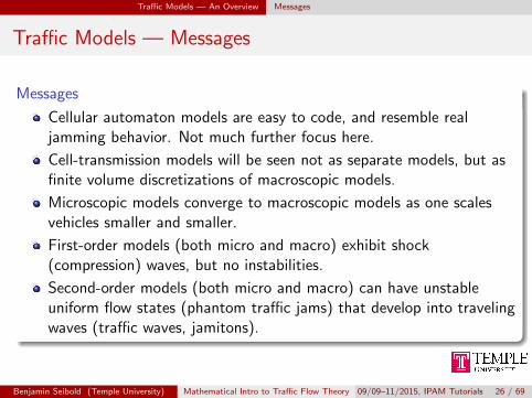
Messages
Cellular automaton models are easy to code, and resemble realjamming behavior. Not much further focus here.
Cell-transmission models will be seen not as separate models, but asfinite volume discretizations of macroscopic models.
Microscopic models converge to macroscopic models as one scalesvehicles smaller and smaller.
First-order models (both micro and macro) exhibit shock(compression) waves, but no instabilities.
Second-order models (both micro and macro) can have unstableuniform flow states (phantom traffic jams) that develop into travelingwaves (traffic waves, jamitons).
Benjamin Seibold (Temple University) Mathematical Intro to Traffic Flow Theory 09/09–11/2015, IPAM Tutorials 26 / 69
The Lighthill-Whitham-Richards Model
Overview
1 Fundamentals of Traffic Flow Theory
2 Traffic Models — An Overview
3 The Lighthill-Whitham-Richards Model
4 Second-Order Macroscopic Models
5 Finite Volume and Cell-Transmission Models
6 Traffic Networks
7 Microscopic Traffic Models
Benjamin Seibold (Temple University) Mathematical Intro to Traffic Flow Theory 09/09–11/2015, IPAM Tutorials 27 / 69
The Lighthill-Whitham-Richards Model Derivation
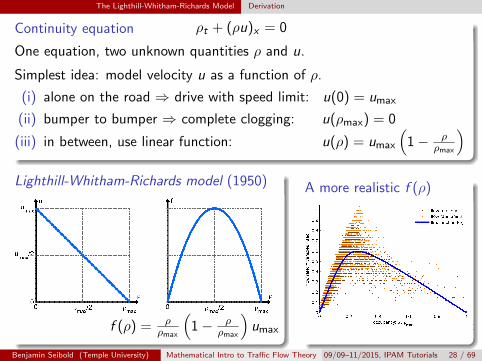
Continuity equation ρt + (ρu)x = 0
One equation, two unknown quantities ρ and u.
Simplest idea: model velocity u as a function of ρ.
(i) alone on the road ⇒ drive with speed limit: u(0) = umax
(ii) bumper to bumper ⇒ complete clogging: u(ρmax) = 0
(iii) in between, use linear function: u(ρ) = umax
(1− ρ
ρmax
)Lighthill-Whitham-Richards model (1950)
f (ρ) = ρρmax
(1− ρ
ρmax
)umax
A more realistic f (ρ)
Benjamin Seibold (Temple University) Mathematical Intro to Traffic Flow Theory 09/09–11/2015, IPAM Tutorials 28 / 69
The Lighthill-Whitham-Richards Model Evolution in Time
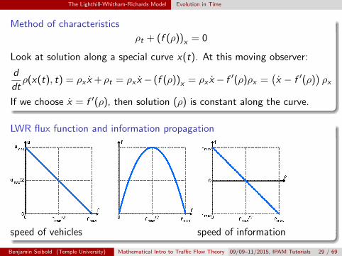
Method of characteristics
ρt + (f (ρ))x = 0
Look at solution along a special curve x(t). At this moving observer:
d
dtρ(x(t), t) = ρx x +ρt = ρx x − (f (ρ))x = ρx x − f ′(ρ)ρx =
(x − f ′(ρ)
)ρx
If we choose x = f ′(ρ), then solution (ρ) is constant along the curve.
LWR flux function and information propagation
speed of vehicles speed of information
Benjamin Seibold (Temple University) Mathematical Intro to Traffic Flow Theory 09/09–11/2015, IPAM Tutorials 29 / 69
The Lighthill-Whitham-Richards Model Evolution in Time
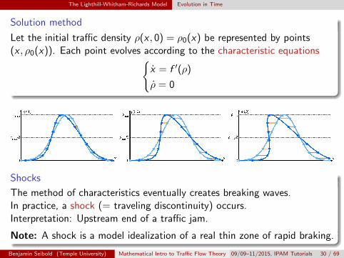
Solution method
Let the initial traffic density ρ(x , 0) = ρ0(x) be represented by points(x , ρ0(x)). Each point evolves according to the characteristic equations{
x = f ′(ρ)
ρ = 0
Shocks
The method of characteristics eventually creates breaking waves.In practice, a shock (= traveling discontinuity) occurs.Interpretation: Upstream end of a traffic jam.
Note: A shock is a model idealization of a real thin zone of rapid braking.
Benjamin Seibold (Temple University) Mathematical Intro to Traffic Flow Theory 09/09–11/2015, IPAM Tutorials 30 / 69
The Lighthill-Whitham-Richards Model Weak Solutions
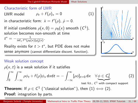
Characteristic form of LWR
LWR model ρt + f (ρ)x = 0 (1)
in characteristic form: x = f ′(ρ), ρ = 0.
If initial conditions ρ(x , 0) = ρ0(x) smooth (C 1),solution becomes non-smooth at timet∗ = − 1
infx f ′′(ρ0(x))ρ′0(x) .
Reality exists for t > t∗, but PDE does not makesense anymore (cannot differentiate discont. function).
Weak solution concept
ρ(x , t) is a weak solution if it satisfies∫ ∞0
∫ ∞−∞
ρφt + f (ρ)φx dxdt = −∫ ∞−∞
[ρφ]t=0 dx ∀φ ∈ C 10︸ ︷︷ ︸
test fct., C1 with compact support
(2)
Theorem: If ρ ∈ C 1 (“classical solution”), then (1) ⇐⇒ (2).
Proof: integration by parts.
Benjamin Seibold (Temple University) Mathematical Intro to Traffic Flow Theory 09/09–11/2015, IPAM Tutorials 31 / 69
The Lighthill-Whitham-Richards Model Weak Solutions
Weak formulation of LWR∫ ∞0
∫ ∞−∞
ρφt + f (ρ)φx dxdt = −∫ ∞−∞
[ρφ]t=0 dx ∀φ ∈ C 10
Every classical (C 1) solution is a weak solution.
In addition, there are discontinuous weak solutions (i.e., with shocks).
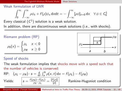
Riemann problem (RP)
ρ0(x) =
{ρL x < 0
ρR x ≥ 0-x
a b
ρL
ρR-s
Speed of shocks
The weak formulation implies that shocks move with a speed such thatthe number of vehicles is conserved:
RP: (ρL − ρR) · s = ddt
∫ ba ρ(x , t) dx = f (ρL)− f (ρR)
Yields: s = f (ρR)−f (ρL)ρR−ρL = [f (ρ)]
[ρ] Rankine-Hugoniot condition
Benjamin Seibold (Temple University) Mathematical Intro to Traffic Flow Theory 09/09–11/2015, IPAM Tutorials 32 / 69
The Lighthill-Whitham-Richards Model Entropy Condition
Weak formulation and Rankine-Hugoniot shock condition∫ ∞0
∫ ∞−∞ρφt + f (ρ)φx dxdt = −
∫ ∞−∞
[ρφ]t=0 dx ∀φ ∈ C 10 ; s =
[f (ρ)]
[ρ]
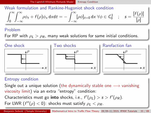
Problem
For RP with ρL > ρR , many weak solutions for same initial conditions.
One shock
-x
6ρ
�
Two shocks
-x
6ρ
�
Rarefaction fan
-x
6ρ
��-
Entropy condition
Single out a unique solution (the dynamically stable one −→ vanishingviscosity limit) via an extra “entropy” condition:
Characteristics must go into shocks, i.e., f ′(ρL) > s > f ′(ρR).
For LWR (f ′′(ρ) < 0): shocks must satisfy ρL < ρR .
Benjamin Seibold (Temple University) Mathematical Intro to Traffic Flow Theory 09/09–11/2015, IPAM Tutorials 33 / 69
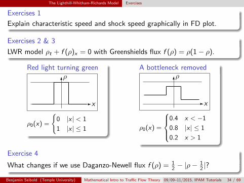
The Lighthill-Whitham-Richards Model Exercises
Exercises 1
Explain characteristic speed and shock speed graphically in FD plot.
Exercises 2 & 3
LWR model ρt + f (ρ)x = 0 with Greenshields flux f (ρ) = ρ(1− ρ).
Red light turning green
-x
6ρ
ρ0(x) =
{0 |x | < 1
1 |x | ≤ 1
A bottleneck removed
-x
6ρ
ρ0(x) =
0.4 x < −1
0.8 |x | ≤ 1
0.2 x > 1
Exercise 4
What changes if we use Daganzo-Newell flux f (ρ) = 12 − |ρ−
12 |?
Benjamin Seibold (Temple University) Mathematical Intro to Traffic Flow Theory 09/09–11/2015, IPAM Tutorials 34 / 69
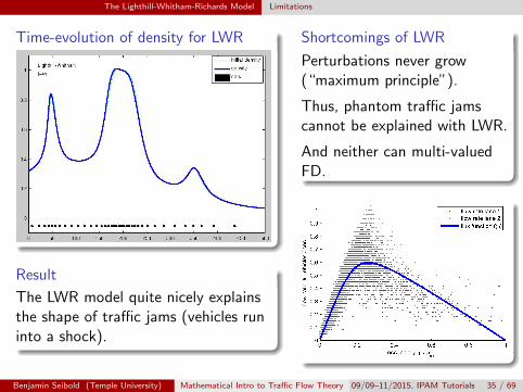
The Lighthill-Whitham-Richards Model Limitations
Time-evolution of density for LWR
Result
The LWR model quite nicely explainsthe shape of traffic jams (vehicles runinto a shock).
Shortcomings of LWR
Perturbations never grow(“maximum principle”).
Thus, phantom traffic jamscannot be explained with LWR.
And neither can multi-valuedFD.
Benjamin Seibold (Temple University) Mathematical Intro to Traffic Flow Theory 09/09–11/2015, IPAM Tutorials 35 / 69

Second-Order Macroscopic Models
Overview
1 Fundamentals of Traffic Flow Theory
2 Traffic Models — An Overview
3 The Lighthill-Whitham-Richards Model
4 Second-Order Macroscopic Models
5 Finite Volume and Cell-Transmission Models
6 Traffic Networks
7 Microscopic Traffic Models
Benjamin Seibold (Temple University) Mathematical Intro to Traffic Flow Theory 09/09–11/2015, IPAM Tutorials 36 / 69
Second-Order Macroscopic Models Payne-Whitham Model
Modeling shortcoming of the LWR model
Vehicles adjust their velocity u instantaneously to the density ρ.Conjecture: real traffic instabilities are caused by vehicles’ inertia.
Payne-Whitham model (1979)
Vehicles at x(t) moves with velocity x(t) = u(x(t), t). Thus itsacceleration is
d
dtu(x(t), t) = ut + ux x = ut + u ux
Model for acceleration: ut + u ux = 1τ (U(ρ)− u)
Here U(ρ) desired velocity (as in previous model), and τ relaxation time.
Full model: {ρt + (ρu)x = 0
ut + u ux =(p(ρ))xρ + 1
τ (U(ρ)− u)
Here p(ρ) traffic pressure (models preventive driving);without this term, vehicles would collide.
Benjamin Seibold (Temple University) Mathematical Intro to Traffic Flow Theory 09/09–11/2015, IPAM Tutorials 37 / 69
Second-Order Macroscopic Models Payne-Whitham Model
Payne-Whitham model{ρt + (ρu)x = 0
ut + u ux +(p(ρ))xρ = 1
τ (U(ρ)− u)
Examples for traffic pressure:
shallow water type: p(ρ) = β2ρ
2 ⇒ pxρ = βρx
singular at ρm: p(ρ) = −β(ρ+ ρm log(1− ρ
ρm))⇒ px
ρ = βρxρm−ρ
Model parameters:
relaxation time τ ( 1τ = aggressiveness of drivers).
anticipation rate β.
System of hyperbolic conservation laws with relaxation term(ρu
)t
+
(u ρ
1ρdpdρ u
)(ρu
)x
=
(0
1τ (U(ρ)− u)
)Characteristic velocities: v = u ± c , with speed of sound: c2 = dp
dρ .
Benjamin Seibold (Temple University) Mathematical Intro to Traffic Flow Theory 09/09–11/2015, IPAM Tutorials 38 / 69
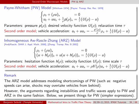
Second-Order Macroscopic Models PW & ARZ
Payne-Whitham (PW) Model [Whitham 1974], [Payne: Transp. Res. Rec. 1979]{ρt + (ρu)x = 0ut + uux + 1
ρp(ρ)x = 1τ (U(ρ)− u)
Parameters: pressure p(ρ); desired velocity function U(ρ); relaxation time τ
Second order model; vehicle acceleration: ut + uux = − p′(ρ)ρ ρx + 1
τ (U(ρ)− u)
Inhomogeneous Aw-Rascle-Zhang (ARZ) Model[Aw&Rascle: SIAM J. Appl. Math. 2000], [Zhang: Transp. Res. B 2002]{
ρt + (ρu)x = 0(u + h(ρ))t + u(u + h(ρ))x = 1
τ (U(ρ)− u)
Parameters: hesitation function h(ρ); velocity function U(ρ); time scale τ
Second order model; vehicle acceleration: ut + uux = ρh′(ρ)ux + 1τ (U(ρ)− u)
Remark
The ARZ model addresses modeling shortcomings of PW (such as: negativespeeds can arise, shocks may overtake vehicles from behind).
However, the arguments regarding instabilities and traffic waves apply to PW andARZ in the same fashion. Below, we present things for PW (simpler expressions).
Benjamin Seibold (Temple University) Mathematical Intro to Traffic Flow Theory 09/09–11/2015, IPAM Tutorials 39 / 69
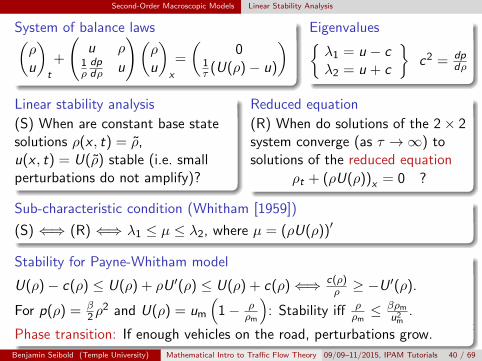
Second-Order Macroscopic Models Linear Stability Analysis
System of balance laws(ρu
)t
+
(u ρ
1ρdpdρ u
)(ρu
)x
=
(0
1τ (U(ρ)− u)
) Eigenvalues{λ1 = u − cλ2 = u + c
}c2 = dp
dρ
Linear stability analysis
(S) When are constant base statesolutions ρ(x , t) = ρ,u(x , t) = U(ρ) stable (i.e. smallperturbations do not amplify)?
Reduced equation
(R) When do solutions of the 2× 2system converge (as τ →∞) tosolutions of the reduced equation
ρt + (ρU(ρ))x = 0 ?
Sub-characteristic condition (Whitham [1959])
(S) ⇐⇒ (R) ⇐⇒ λ1 ≤ µ ≤ λ2, where µ = (ρU(ρ))′
Stability for Payne-Whitham model
U(ρ)− c(ρ) ≤ U(ρ) + ρU ′(ρ) ≤ U(ρ) + c(ρ)⇐⇒ c(ρ)ρ ≥ −U
′(ρ).
For p(ρ) = β2ρ
2 and U(ρ) = um
(1− ρ
ρm
): Stability iff ρ
ρm≤ βρm
u2m
.
Phase transition: If enough vehicles on the road, perturbations grow.
Benjamin Seibold (Temple University) Mathematical Intro to Traffic Flow Theory 09/09–11/2015, IPAM Tutorials 40 / 69
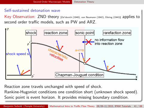
Second-Order Macroscopic Models Detonation Theory
Self-sustained detonation wave
Key Observation: ZND theory [Zel’dovich (1940), von Neumann (1942), Doring (1943)] applies tosecond order traffic models, such as PW and ARZ.
Reaction zone travels unchanged with speed of shock.Rankine-Hugoniot conditions one condition short (unknown shock speed).Sonic point is event horizon. It provides missing boundary condition.
Benjamin Seibold (Temple University) Mathematical Intro to Traffic Flow Theory 09/09–11/2015, IPAM Tutorials 41 / 69
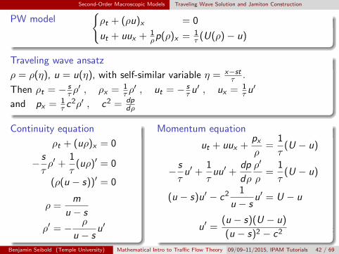
Second-Order Macroscopic Models Traveling Wave Solution and Jamiton Construction
PW model{ρt + (ρu)x = 0
ut + uux + 1ρp(ρ)x = 1
τ (U(ρ)− u)
Traveling wave ansatz
ρ = ρ(η), u = u(η), with self-similar variable η = x−stτ .
Then ρt = − sτ ρ′ , ρx = 1
τ ρ′ , ut = − s
τ u′ , ux = 1
τ u′
and px = 1τ c
2ρ′ , c2 = dpdρ
Continuity equation
ρt + (uρ)x = 0
− s
τρ′ +
1
τ(uρ)′ = 0
(ρ(u − s))′ = 0
ρ =m
u − s
ρ′ = − ρ
u − su′
Momentum equation
ut + uux +pxρ
=1
τ(U − u)
− s
τu′ +
1
τuu′ +
dp
dρ
ρ′
ρ=
1
τ(U − u)
(u − s)u′ − c2 1
u − su′ = U − u
u′ =(u − s)(U − u)
(u − s)2 − c2
Benjamin Seibold (Temple University) Mathematical Intro to Traffic Flow Theory 09/09–11/2015, IPAM Tutorials 42 / 69
Second-Order Macroscopic Models Traveling Wave Solution and Jamiton Construction
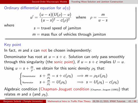
Ordinary differential equation for u(η)
u′ =(u − s)(U(ρ)− u)
(u − s)2 − c(ρ)2where ρ =
m
u − swhere
s = travel speed of jamiton
m = mass flux of vehicles through jamiton
Key point
In fact, m and s can not be chosen independently:
Denominator has root at u = s + c . Solution can only pass smoothlythrough this singularity (the sonic point), if u = s + c implies U = u.
Using u = s + mρ , we obtain for this sonic density ρS that:{
Denominator s + mρS
= s + c(ρS) =⇒ m = ρSc(ρS)
Numerator s + mρS
= U(ρS) =⇒ s = U(ρS)− c(ρS)
Algebraic condition (Chapman-Jouguet condition [Chapman, Jouguet (1890)]) thatrelates m and s (and ρS).
Benjamin Seibold (Temple University) Mathematical Intro to Traffic Flow Theory 09/09–11/2015, IPAM Tutorials 43 / 69
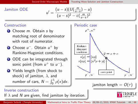
Second-Order Macroscopic Models Traveling Wave Solution and Jamiton Construction
Jamiton ODEu′ =
(u − s)(U( mu−s )− u)
(u − s)2 − c( mu−s )2
Construction1 Choose m. Obtain s by
matching root of denominatorwith root of numerator.
2 Choose u−. Obtain u+ byRankine-Hugoniot conditions.
3 ODE can be integrated throughsonic point (from u+ to u−).
4 Yields length (from shock toshock) of jamiton, λ, and
number of cars, N =∫ λ
0 ρ(x)dx .
Periodic case
Inverse constructionIf λ and N are given, find jamiton by iteration.
jamiton length = O(τ)
Benjamin Seibold (Temple University) Mathematical Intro to Traffic Flow Theory 09/09–11/2015, IPAM Tutorials 44 / 69
Second-Order Macroscopic Models Jamitons in an Experiment
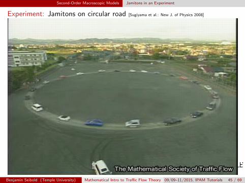
Experiment: Jamitons on circular road [Sugiyama et al.: New J. of Physics 2008]
Benjamin Seibold (Temple University) Mathematical Intro to Traffic Flow Theory 09/09–11/2015, IPAM Tutorials 45 / 69
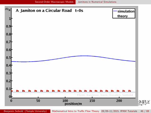
Second-Order Macroscopic Models Jamitons in Numerical Simulations
Benjamin Seibold (Temple University) Mathematical Intro to Traffic Flow Theory 09/09–11/2015, IPAM Tutorials 46 / 69
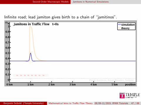
Second-Order Macroscopic Models Jamitons in Numerical Simulations
Infinite road; lead jamiton gives birth to a chain of “jamitinos”.
Benjamin Seibold (Temple University) Mathematical Intro to Traffic Flow Theory 09/09–11/2015, IPAM Tutorials 47 / 69
Second-Order Macroscopic Models Jamitons in the Fundamental Diagram
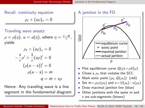
Recall: continuity equation
ρt + (uρ)x = 0
Traveling wave ansatz
ρ = ρ(η), u = u(η), where η = x−stτ ,
yields
ρt + (uρ)x = 0
− s
τρ′ +
1
τ(uρ)′ = 0
(ρ(u − s))′ = 0
ρ(u − s) = m
q = m + sρ
Hence: Any traveling wave is a linesegment in the fundamental diagram.
A jamiton in the FD
ρR
ρM
ρS
ρ−ρ+
ρ
Q(ρ
)
equilibrium curvesonic pointmaximal jamitonactual jamiton
• Plot equilibrium curve Q(ρ)=ρU(ρ)
• Chose a ρS that violates the SCC
• Mark sonic point (ρS,Q(ρS)) (red)
• Set m=ρSc(ρS) and s =U(ρS)−c(ρS)
• Draw maximal jamiton line (blue)
• Other jamitons with the same m ands are sub-segments (brown)
Benjamin Seibold (Temple University) Mathematical Intro to Traffic Flow Theory 09/09–11/2015, IPAM Tutorials 48 / 69
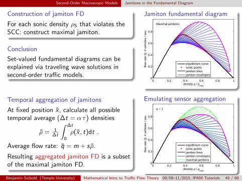
Second-Order Macroscopic Models Jamitons in the Fundamental Diagram
Construction of jamiton FD
For each sonic density ρS that violates theSCC: construct maximal jamiton.
Conclusion
Set-valued fundamental diagrams can beexplained via traveling wave solutions insecond-order traffic models.
Temporal aggregation of jamitons
At fixed position x , calculate all possibletemporal average (∆t = α τ) densities
ρ = 1∆t
∫ ∆t
0
ρ(x , t)dt .
Average flow rate: q = m + s ρ.
Resulting aggregated jamiton FD is a subsetof the maximal jamiton FD.
Jamiton fundamental diagram
0 0.2 0.4 0.6 0.8 10
0.2
0.4
0.6
0.8
Maximal jamitons
density ρ / ρmax
flow
rat
e Q
: # v
ehic
les
/ sec
.
equilibrium curvesonic pointsjamiton linesjamiton envelopes
Emulating sensor aggregation
0 0.2 0.4 0.6 0.8 10
0.2
0.4
0.6
0.8
α = 1
density ρ / ρmax
flow
rat
e Q
: # v
ehic
les
/ sec
.
equilibrium curvesonic pointsjamiton linesjamiton envelopesmaximal jamitons
Benjamin Seibold (Temple University) Mathematical Intro to Traffic Flow Theory 09/09–11/2015, IPAM Tutorials 49 / 69
Second-Order Macroscopic Models Jamitons in the Fundamental Diagram
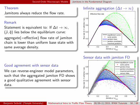
Theorem
Jamitons always reduce the flow rate.
Remark
Statement is equivalent to: If ∆t →∞,(ρ, q) lies below the equilibrium curve:
aggregate(=effective) flow rate of jamitonchain is lower than uniform base state withsame average density.
Good agreement with sensor data
We can reverse-engineer model parameters,such that the aggregated jamiton FD showsa good qualitative agreement with sensordata.
Infinite aggregation (∆t →∞)
0 0.2 0.4 0.6 0.8 10
0.2
0.4
0.6
0.8
Effective flow rate
density ρ / ρmax
flow
rat
e Q
: # v
ehic
les
/ sec
.
equilibrium curvesonic pointsjamiton linesjamiton envelopesmaximal jamitons
Sensor data with jamiton FD
0 0.2 0.4 0.6 0.8 10
0.2
0.4
0.6
0.8
density ρ / ρmax
flow
rat
e Q
: # v
ehic
les
/ sec
.
equilibrium curvesonic pointsjamiton linesjamiton envelopesmaximal jamitonssensor data
Benjamin Seibold (Temple University) Mathematical Intro to Traffic Flow Theory 09/09–11/2015, IPAM Tutorials 50 / 69
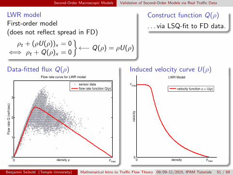
Second-Order Macroscopic Models Validation of Second-Order Models via Real Traffic Data
LWR modelFirst-order model(does not reflect spread in FD)
ρt + (ρU(ρ))x = 0⇐⇒ ρt + Q(ρ)x = 0
}←− Q(ρ) = ρU(ρ)
Construct function Q(ρ)
. . . via LSQ-fit to FD data.
Data-fitted flux Q(ρ)
0
1
2
3
density ρ
Flo
w r
ate
Q (
veh/s
ec)
0 ρmax
Flow rate curve for LWR model
sensor data
flow rate function Q(ρ)
Induced velocity curve U(ρ)LWR Model
density
velo
city
0 ρmax
0
vmax
velocity function u = U(ρ)
Benjamin Seibold (Temple University) Mathematical Intro to Traffic Flow Theory 09/09–11/2015, IPAM Tutorials 51 / 69
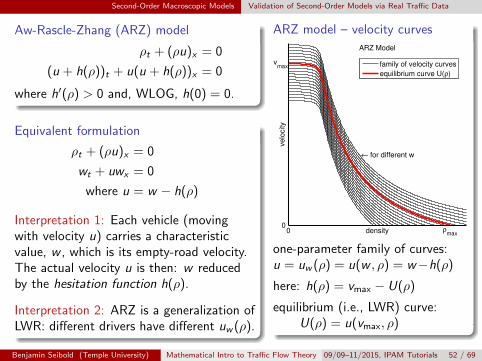
Second-Order Macroscopic Models Validation of Second-Order Models via Real Traffic Data
Aw-Rascle-Zhang (ARZ) model
ρt + (ρu)x = 0
(u + h(ρ))t + u(u + h(ρ))x = 0
where h′(ρ) > 0 and, WLOG, h(0) = 0.
Equivalent formulation
ρt + (ρu)x = 0
wt + uwx = 0
where u = w − h(ρ)
Interpretation 1: Each vehicle (movingwith velocity u) carries a characteristicvalue, w , which is its empty-road velocity.The actual velocity u is then: w reducedby the hesitation function h(ρ).
Interpretation 2: ARZ is a generalization ofLWR: different drivers have different uw (ρ).
ARZ model – velocity curves
ARZ Model
density
velo
city
0 ρmax
0
vmax
← for different w
family of velocity curves
equilibrium curve U(ρ)
one-parameter family of curves:u = uw (ρ) = u(w , ρ) = w−h(ρ)
here: h(ρ) = vmax − U(ρ)
equilibrium (i.e., LWR) curve:U(ρ) = u(vmax, ρ)
Benjamin Seibold (Temple University) Mathematical Intro to Traffic Flow Theory 09/09–11/2015, IPAM Tutorials 52 / 69
Second-Order Macroscopic Models Validation of Second-Order Models via Real Traffic Data
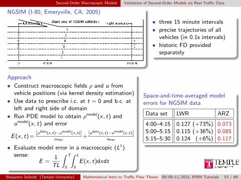
NGSIM (I-80, Emeryville, CA; 2005)
• three 15 minute intervals
• precise trajectories of allvehicles (in 0.1s intervals)
• historic FD providedseparately
Approach
• Construct macroscopic fields ρ and u fromvehicle positions (via kernel density estimation)
• Use data to prescribe i.c. at t = 0 and b.c. atleft and right side of domain
• Run PDE model to obtain ρmodel(x , t) andumodel(x , t) and error
E(x , t)=|ρdata(x,t)−ρmodel(x,t)|
ρmax+|udata(x,t)−umodel(x,t)|
umax
• Evaluate model error in a macroscopic (L1)sense:
E =1
TL
∫ T
0
∫ L
0
E(x , t)dxdt
Space-and-time-averaged modelerrors for NGSIM data
Data set LWR ARZ
4:00–4:15 0.127 (+73%) 0.0735:00–5:15 0.115 (+36%) 0.0855:15–5:30 0.124 (+6%) 0.117
Benjamin Seibold (Temple University) Mathematical Intro to Traffic Flow Theory 09/09–11/2015, IPAM Tutorials 53 / 69
Finite Volume and Cell-Transmission Models
Overview
1 Fundamentals of Traffic Flow Theory
2 Traffic Models — An Overview
3 The Lighthill-Whitham-Richards Model
4 Second-Order Macroscopic Models
5 Finite Volume and Cell-Transmission Models
6 Traffic Networks
7 Microscopic Traffic Models
Benjamin Seibold (Temple University) Mathematical Intro to Traffic Flow Theory 09/09–11/2015, IPAM Tutorials 54 / 69
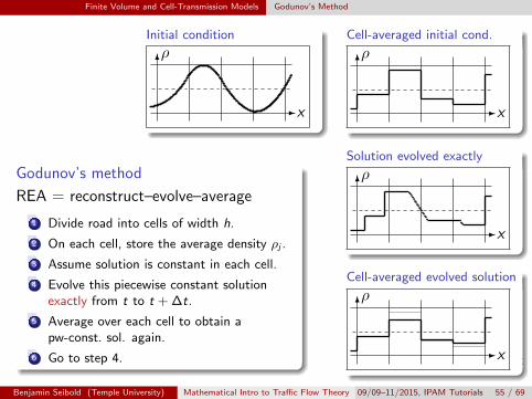
Finite Volume and Cell-Transmission Models Godunov’s Method
Initial condition
-x
6ρ
Cell-averaged initial cond.
-x
6ρ
Godunov’s method
REA = reconstruct–evolve–average
1 Divide road into cells of width h.
2 On each cell, store the average density ρj .
3 Assume solution is constant in each cell.
4 Evolve this piecewise constant solutionexactly from t to t + ∆t.
5 Average over each cell to obtain apw-const. sol. again.
6 Go to step 4.
Solution evolved exactly
-x
6ρ
Cell-averaged evolved solution
-x
6ρ
Benjamin Seibold (Temple University) Mathematical Intro to Traffic Flow Theory 09/09–11/2015, IPAM Tutorials 55 / 69
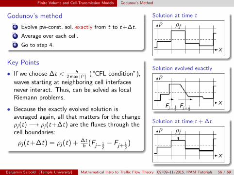
Finite Volume and Cell-Transmission Models Godunov’s Method
Godunov’s method
4 Evolve pw-const. sol. exactly from t to t+∆t.
5 Average over each cell.
6 Go to step 4.
Key Points
• If we choose ∆t < h2 max |f ′| (“CFL condition”),
waves starting at neighboring cell interfacesnever interact. Thus, can be solved as localRiemann problems.
• Because the exactly evolved solution isaveraged again, all that matters for the changeρj(t) −→ ρj(t+∆t) are the fluxes through thecell boundaries:
ρj(t+∆t) = ρj(t) + ∆th (Fj− 1
2− Fj+ 1
2)
Solution at time t
-x
6ρ ρj
Solution evolved exactly
-x
6ρ
-
Fj− 12
-
Fj+ 12
Solution at time t + ∆t
-x
6ρ ρj
?
Benjamin Seibold (Temple University) Mathematical Intro to Traffic Flow Theory 09/09–11/2015, IPAM Tutorials 56 / 69
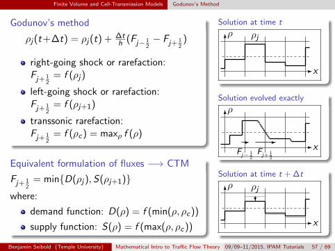
Finite Volume and Cell-Transmission Models Godunov’s Method
Godunov’s method
ρj(t+∆t) = ρj(t) + ∆th (Fj− 1
2− Fj+ 1
2)
right-going shock or rarefaction:Fj+ 1
2= f (ρj)
left-going shock or rarefaction:Fj+ 1
2= f (ρj+1)
transsonic rarefaction:Fj+ 1
2= f (ρc) = maxρ f (ρ)
Equivalent formulation of fluxes −→ CTM
Fj+ 12
= min{D(ρj), S(ρj+1)}where:
demand function: D(ρ) = f (min(ρ, ρc))
supply function: S(ρ) = f (max(ρ, ρc))
Solution at time t
-x
6ρ ρj
Solution evolved exactly
-x
6ρ
-
Fj− 12
-
Fj+ 12
Solution at time t + ∆t
-x
6ρ ρj
?
Benjamin Seibold (Temple University) Mathematical Intro to Traffic Flow Theory 09/09–11/2015, IPAM Tutorials 57 / 69
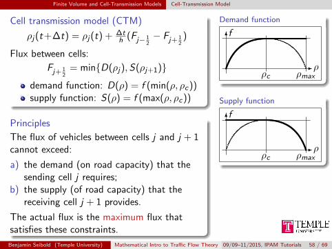
Finite Volume and Cell-Transmission Models Cell-Transmission Model
Cell transmission model (CTM)
ρj(t+∆t) = ρj(t) + ∆th (Fj− 1
2− Fj+ 1
2)
Flux between cells:
Fj+ 12
= min{D(ρj),S(ρj+1)}
demand function: D(ρ) = f (min(ρ, ρc))supply function: S(ρ) = f (max(ρ, ρc))
Principles
The flux of vehicles between cells j and j + 1cannot exceed:
a) the demand (on road capacity) that thesending cell j requires;
b) the supply (of road capacity) that thereceiving cell j + 1 provides.
The actual flux is the maximum flux thatsatisfies these constraints.
Demand function
-ρ
6f
ρc ρmax
Supply function
-ρ
6f
ρc ρmax
Benjamin Seibold (Temple University) Mathematical Intro to Traffic Flow Theory 09/09–11/2015, IPAM Tutorials 58 / 69
Finite Volume and Cell-Transmission Models Convergence Results
Convergence of the Godunov method (or CTM)
As ∆t = Ch→ 0, the sequence of approximate solutions converges(in L1) to the unique weak entropy solution of the LWR modelρt + f (ρ)x = 0.
For any fixed ∆t and h, the temporal evolution that Godunov=CTMprovides is only an approximation to the LWR model.
To leading order, Godunov=CTM solutions behave like solutions ofthe “modified equation” ρt + f (ρ)x = chρxx .
Hence, the error between Godunov=CTM and LWR scales like O(h);first-order numerical scheme.
Also, shocks get smeared out over several cells.
Other, more accurate (high-order) numerical schemes for LWR exist(MUSCL, discontinuous Galerkin, etc.). These are more complicated.
CTMs can also be cast for second-order traffic models.
Benjamin Seibold (Temple University) Mathematical Intro to Traffic Flow Theory 09/09–11/2015, IPAM Tutorials 59 / 69
Traffic Networks
Overview
1 Fundamentals of Traffic Flow Theory
2 Traffic Models — An Overview
3 The Lighthill-Whitham-Richards Model
4 Second-Order Macroscopic Models
5 Finite Volume and Cell-Transmission Models
6 Traffic Networks
7 Microscopic Traffic Models
Benjamin Seibold (Temple University) Mathematical Intro to Traffic Flow Theory 09/09–11/2015, IPAM Tutorials 60 / 69
Traffic Networks Cell-Transmission Model
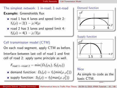
The simplest network: 1 in-road; 1 out-road
Example: Greenshields flux
road 1 has 4 lanes and speed limit 2:f1(ρ) = 2(1− ρ/4)ρ
road 2 has 3 lanes and speed limit 4:f2(ρ) = 4(1− ρ/3)ρ
Cell transmission model (CTM)
On each road segment, apply CTM as before.
Interface between last cell of road 1 and firstcell of road 2: apply same principle as well.
Froad 1→road 2 = min{D1(ρ1),S2(ρ2)}
demand function: D1(ρ) = f1(min(ρ, ρ1c))
supply function: S2(ρ) = f2(max(ρ, ρ2c))
Demand function
-ρ
6f
2
2 4
Supply function
-ρ
6f
3
1.5 3
Nice
As simple to code as thebasic CTM.
Benjamin Seibold (Temple University) Mathematical Intro to Traffic Flow Theory 09/09–11/2015, IPAM Tutorials 61 / 69
Traffic Networks Generalized Riemann Problem
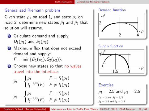
Generalized Riemann problem
Given state ρ1 on road 1, and state ρ2 onroad 2, determine new states ρ1 and ρ2 thatsolution will assume.
1 Calculate demand and supply:D1(ρ1) and S2(ρ2).
2 Maximum flux that does not exceeddemand and supply:F = min{D1(ρ1),S2(ρ2)}.
3 Choose new states so that no wavestravel into the interface:
ρ1 =
{ρ1 F = f1(ρ1)
f −1,⊕1 (F ) F 6= f1(ρ1)
ρ2 =
{ρ2 F = f2(ρ2)
f −1,2 (F ) F 6= f2(ρ2)
Demand function
-ρ
6f
2
2 4
Supply function
-ρ
6f
3
1.5 3
Exercise
ρ1 = 2.5 and ρ2 = 2.5D1 = 2 and S2 = 5/3
ρ1 ≈ 2.8 and ρ2 = 2.5
Benjamin Seibold (Temple University) Mathematical Intro to Traffic Flow Theory 09/09–11/2015, IPAM Tutorials 62 / 69
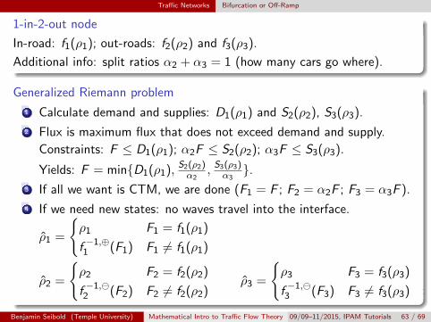
Traffic Networks Bifurcation or Off-Ramp
1-in-2-out node
In-road: f1(ρ1); out-roads: f2(ρ2) and f3(ρ3).
Additional info: split ratios α2 + α3 = 1 (how many cars go where).
Generalized Riemann problem
1 Calculate demand and supplies: D1(ρ1) and S2(ρ2), S3(ρ3).
2 Flux is maximum flux that does not exceed demand and supply.
Constraints: F ≤ D1(ρ1); α2F ≤ S2(ρ2); α3F ≤ S3(ρ3).
Yields: F = min{D1(ρ1), S2(ρ2)α2
, S3(ρ3)α3}.
3 If all we want is CTM, we are done (F1 = F ; F2 = α2F ; F3 = α3F ).
4 If we need new states: no waves travel into the interface.
ρ1 =
{ρ1 F1 = f1(ρ1)
f −1,⊕1 (F1) F1 6= f1(ρ1)
ρ2 =
{ρ2 F2 = f2(ρ2)
f −1,2 (F2) F2 6= f2(ρ2)
ρ3 =
{ρ3 F3 = f3(ρ3)
f −1,3 (F3) F3 6= f3(ρ3)
Benjamin Seibold (Temple University) Mathematical Intro to Traffic Flow Theory 09/09–11/2015, IPAM Tutorials 63 / 69
Traffic Networks Bifurcation or Off-Ramp
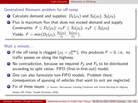
Generalized Riemann problem for off-ramp
1 Calculate demand and supplies: D1(ρ1) and S2(ρ2), S3(ρ3).
2 Flux is maximum flux that does not exceed demand and supply.
Constraints: F ≤ D1(ρ1); α2F ≤ S2(ρ2); α3F ≤ S3(ρ3).
Yields: F = min{D1(ρ1), S2(ρ2)α2
, S3(ρ3)α3}.
Wait a minute. . .
1 If the off-ramp is clogged (ρ3 = ρmax3 ), this produces F = 0, i.e., no
traffic passes on along the highway.
2 No contradiction, because we required F2 and F3 to be distributedaccording to split ratios: FIFO (first-in-first-out) model.
3 One can also formulate non-FIFO models. Problem there:consequences of queuing of vehicles that want to exit are neglected.
4 Fix of these issues: [J. Somers: Macroscopic Coupling Conditions with Partial Blocking for Highway
Ramps, MS Thesis, Temple University, 2015].
Benjamin Seibold (Temple University) Mathematical Intro to Traffic Flow Theory 09/09–11/2015, IPAM Tutorials 64 / 69
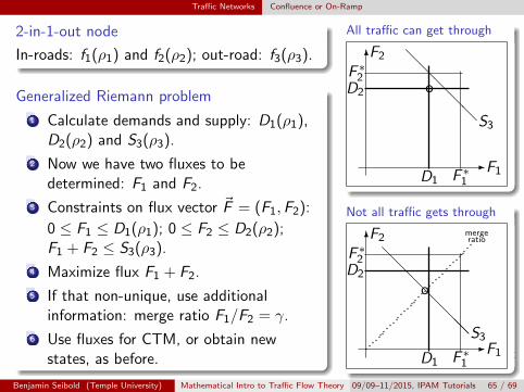
Traffic Networks Confluence or On-Ramp
2-in-1-out node
In-roads: f1(ρ1) and f2(ρ2); out-road: f3(ρ3).
Generalized Riemann problem
1 Calculate demands and supply: D1(ρ1),D2(ρ2) and S3(ρ3).
2 Now we have two fluxes to bedetermined: F1 and F2.
3 Constraints on flux vector ~F = (F1,F2):
0 ≤ F1 ≤ D1(ρ1); 0 ≤ F2 ≤ D2(ρ2);F1 + F2 ≤ S3(ρ3).
4 Maximize flux F1 + F2.
5 If that non-unique, use additionalinformation: merge ratio F1/F2 = γ.
6 Use fluxes for CTM, or obtain newstates, as before.
All traffic can get through
-F1
6F2
F ∗1
F ∗2
D1
D2
@@@@@S3
o
Not all traffic gets through
-F1
6F2
F ∗1
F ∗2
D1
D2
@@@@@@@S3
mergeratio
o
Benjamin Seibold (Temple University) Mathematical Intro to Traffic Flow Theory 09/09–11/2015, IPAM Tutorials 65 / 69
Traffic Networks General Networks
General Networks
The presented 1-in-1-out, 1-in-2-out, and 2-in-1-out nodes alreadyenable us to put together large road networks.
Can use CTM to compute LWR solutions on such a network.
Even for the simple on- and off-ramp case, there is still somemodeling and validation work to be done with regards to the questionwhich choices of fluxes are most realistic.
The general n-in-m-out case can be treated similarly. However, theconstrained flux maximization leads to a linear program that mayneed to be solved numerically (can be costly).
Second-order models: coupling conditions for the ARZ model havebeen developed, albeit not for the most general case.
Benjamin Seibold (Temple University) Mathematical Intro to Traffic Flow Theory 09/09–11/2015, IPAM Tutorials 66 / 69
Microscopic Traffic Models
Overview
1 Fundamentals of Traffic Flow Theory
2 Traffic Models — An Overview
3 The Lighthill-Whitham-Richards Model
4 Second-Order Macroscopic Models
5 Finite Volume and Cell-Transmission Models
6 Traffic Networks
7 Microscopic Traffic Models
Benjamin Seibold (Temple University) Mathematical Intro to Traffic Flow Theory 09/09–11/2015, IPAM Tutorials 67 / 69
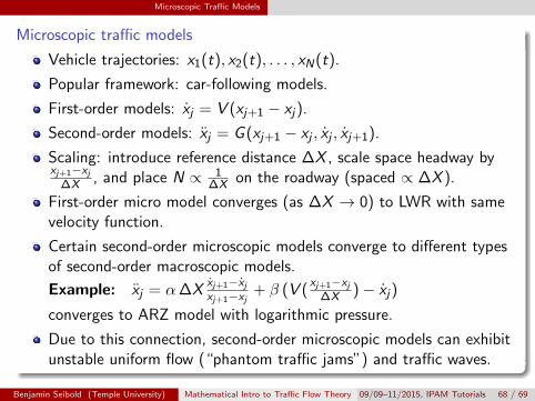
Microscopic Traffic Models
Microscopic traffic models
Vehicle trajectories: x1(t), x2(t), . . . , xN(t).
Popular framework: car-following models.
First-order models: xj = V (xj+1 − xj).
Second-order models: xj = G (xj+1 − xj , xj , xj+1).
Scaling: introduce reference distance ∆X , scale space headway byxj+1−xj
∆X , and place N ∝ 1∆X on the roadway (spaced ∝ ∆X ).
First-order micro model converges (as ∆X → 0) to LWR with samevelocity function.
Certain second-order microscopic models converge to different typesof second-order macroscopic models.
Example: xj = α∆Xxj+1−xjxj+1−xj + β (V (
xj+1−xj∆X )− xj)
converges to ARZ model with logarithmic pressure.
Due to this connection, second-order microscopic models can exhibitunstable uniform flow (“phantom traffic jams”) and traffic waves.
Benjamin Seibold (Temple University) Mathematical Intro to Traffic Flow Theory 09/09–11/2015, IPAM Tutorials 68 / 69
Microscopic Traffic Models
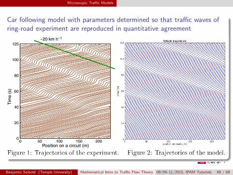
Car following model with parameters determined so that traffic waves ofring-road experiment are reproduced in quantitative agreement
Benjamin Seibold (Temple University) Mathematical Intro to Traffic Flow Theory 09/09–11/2015, IPAM Tutorials 69 / 69