Mon. Not. R. Astron. Soc. 000, 000–000 (0000) Printed 3 March 2010 (MN LATEX style file v2.2)

A mass-loss rate determination for ζ Puppis from the

quantitative analysis of X-ray emission line profiles

David H. Cohen,1? Maurice A. Leutenegger,2 Emma E. Wollman,1,3

Janos Zsargo,4,5 D. John Hillier,4 Richard H. D. Townsend,6,7 Stanley P. Owocki,61Swarthmore College, Department of Physics and Astronomy, Swarthmore, Pennsylvania 19081, USA2NASA/Goddard Space Flight Center, Laboratory for High Energy Astrophysics, Code 622, Greenbelt, Maryland 20771, USA3California Institute of Technology, Department of Physics, Pasadena, California 91125, USA4University of Pittsburgh, Department of Physics and Astronomy, 3941 O’Hara St., Pittsburgh, Pennsylvania 15260, USA5Instituto Politecnico Nacional, Escuela Superior de Fisica y Matematicas, C.P. 07738, Mexico, D. F., Mexico6University of Delaware, Bartol Research Institute, Newark, Delaware 19716, USA7University of Wisconsin, Department of Astronomy, Madison, 475 N. Charter St., Madison, Wisconsin 53706, USA

3 March 2010

ABSTRACT

We fit every emission line in the high-resolution Chandra grating spectrum ofζ Pup with an empirical line profile model that accounts for the effects of Dopplerbroadening and attenuation by the bulk wind. For each of sixteen lines or line com-plexes that can be reliably measured, we determine a best-fitting fiducial optical depth,

τ∗ ≡ κM/4πR∗v∞, and place confidence limits on this parameter. These sixteen linesinclude seven that have not previously been reported on in the literature. The ex-tended wavelength range of these lines allows us to infer, for the first time, a clearincrease in τ∗ with line wavelength, as expected from the wavelength increase of bound-free absorption opacity. The small overall values of τ∗, reflected in the rather modestasymmetry in the line profiles, can moreover all be fit simultaneously by simply as-suming a moderate mass-loss rate of 3.5 ± 0.3 × 10−6 M¯ yr−1, without any needto invoke porosity effects in the wind. The quoted uncertainty is statistical, but thelargest source of uncertainty in the derived mass-loss rate is due to the uncertaintyin the elemental abundances of ζ Pup, which affects the continuum opacity of thewind, and which we estimate to be a factor of two. Even so, the mass-loss rate we findis significantly below the most recent smooth-wind Hα mass-loss rate determinationsfor ζ Pup, but is in line with newer determinations that account for small-scale windclumping. If ζ Pup is representative of other massive stars, these results will haveimportant implications for stellar and galactic evolution.

Key words: stars: early-type – stars: mass-loss – stars: winds, outflows – stars:individual: ζ Pup – X-rays: stars

1 INTRODUCTION

Massive stars can lose a significant fraction of their orig-inal mass during their short lifetimes due to their strong,radiation-driven stellar winds. Accurate determinations ofthese stars’ mass-loss rates are therefore important from anevolutionary point of view, as well as for understanding theradiative driving process itself. Massive star winds are alsoan important source of energy, momentum, and (chemicallyenriched) matter deposition into the interstellar medium,

? E-mail: cohen@astro.swarthmore.edu

making accurate mass-loss rate determinations importantfrom a galactic perspective.

A consensus appeared to be reached by the late 1990sthat the mass-loss rates of O stars were accurately knownobservationally and theoretically, using the modified (Paul-drach et al. 1986) CAK (Castor et al. 1975) theory of line-driven stellar winds. This understanding was thought to begood enough that UV observations of spectral signatures oftheir winds could be used to determine their luminositieswith sufficient accuracy to make extragalactic O stars stan-dard candles (Puls et al. 1996).

This consensus has unraveled in the last few years,mostly from the observational side, where a growing appre-

c© 0000 RAS

2 D. Cohen et al.

ciation of wind clumping – an effect whose importance haslong been recognized (Eversberg et al. 1998; Hillier & Miller1999; Hamann & Koesterke 1999) – has led to a re-evaluationof mass-loss rate diagnostics, including Hα emission, radioand IR free-free emission, and UV absorption (Bouret et al.2005; Puls et al. 2006; Fullerton et al. 2006). Accounting forsmall-scale clumping that affects density squared emissiondiagnostics – and also ionization balance and thus ionic col-umn density diagnostics like UV resonance lines – leads toa downward revision of mass-loss rates by a factor of sev-eral, with a fair amount of controversy over the actual factor(Hamann et al. 2008; Puls et al. 2008).

X-ray emission line profile analysis provides a good andindependent way to measure the mass-loss rates of O stars.Like the UV absorption line diagnostics, X-ray emission pro-file diagnostics are sensitive to the wind column densityand thus are not directly affected by clumping in the waydensity-squared diagnostics are. Unlike the UV absorptionline diagnostics, however, X-ray profile analysis is not verysensitive to the ionization balance; moreover, as it relies oncontinuum opacity rather than line opacity, it is not sub-ject to the uncertainty associated with saturated absorptionlines that hamper the interpretation of the UV diagnostics.

In this paper, we apply a quantitative line profile anal-ysis to the Chandra grating spectrum of the early O super-giant, ζ Pup, one of the nearest O stars to the Earth and astar that has long been used as a canonical example of anearly O star with a strong radiation-driven wind. Previousanalysis of the same Chandra data has established that thekinematics of the X-ray emitting plasma, as diagnosed by theline widths, are in good agreement with wind-shock theory,and that there are modest signatures of attenuation of theX-rays by the dominant cold wind component in which theshock-heated X-ray emitting plasma is embedded (Krameret al. 2003).

The work presented here goes beyond the profile anal-ysis reported in that paper in several respects. We analyzemany lines left out of the original study that are weak, butwhich carry a significant amount of information. We betteraccount for line blends and are careful to exclude those lineswhere blending cannot be adequately modelled. We modelthe continuum emission underlying each line separately fromthe line itself. We use a realistic model of the spectrometers’responses and the telescope and detector effective area. Andwe include the High Energy Grating (HEG) spectral data,where appropriate, to augment the higher signal-to-noiseMedium Energy Grating (MEG) data that Kramer et al.(2003) reported on.

Implementing all of these improvements enables us toderive highly reliable values of the fiducial wind opticaldepth parameter, τ∗ ≡ κM/4πR∗v∞, for each of sixteenemission lines or line complexes in the Chandra grating spec-trum of ζ Pup. Using a model of the wavelength-dependentwind opacity, κ, and values for the star’s radius, R∗, andwind terminal velocity, v∞, derived from UV and opticalobservations, we can fit a value of the mass-loss rate, M, tothe ensemble of τ∗ values, and thereby determine the mass-loss rate of ζ Pup based on the observed X-ray emission lineprofiles.

In doing this, we also can verify that the wavelength-dependence of the optical depth values – derived separatelyfor each individual line – is consistent with that of the

atomic opacity of the bulk wind, rather than the gray opac-ity that would, for example, be obtained from an extremelyporous wind (Oskinova et al. 2006; Owocki & Cohen 2006).While a moderate porosity might reduce somewhat the ef-fective absorption while still retaining some wavelength de-pendence, for simplicity our analysis here assumes a purelyatomic opacity set by photoelectric absorption, with no re-duction from porosity. This assumption is justified by thelarge porosity lengths required for any appreciable poros-ity effect on line profile shapes (Owocki & Cohen 2006)and the very small-scale clumping in state-of-the-art two-dimensional radiation hydrodynamics simulations (Dessart& Owocki 2003). Furthermore, preliminary results indicatethat profile models that explicitly include porosity are notfavored over ones that do not (Cohen et al. 2008). We willextend this result in a forthcoming paper but do not ad-dress the effect of porosity on individual line profile shapesdirectly in the current work.

The paper is organized as follows: We begin by describ-ing the Chandra data set and defining a sample of well be-haved emission lines for our analysis in §2. We briefly eval-uate the stellar and wind properties of ζ Pup in §3. In §4we describe the empirical profile model for X-ray emissionlines and report on the fits to the sixteen usable lines andline complexes in the spectrum. We discuss the implicationsof the profile model fitting results in §5, and summarize ourconclusions in §6.

2 THE Chandra GRATING SPECTRUM

All the data we use in this paper were taken on 28-29March 2000 in a single, 68 ks observation using the Chandra

High-Energy Transmission Grating Spectrometer (HETGS)in conjunction with the Advanced CCD Imaging Spectrom-eter (ACIS) detector in spectroscopy mode (Canizares et al.2005). This is a photon counting instrument with an ex-tremely low background and high spatial resolution (≈ 1′′).The first-order grating spectra we analyzed have a total of21,684 counts, the vast majority of which are in emissionlines, as can be seen in Fig. 1. We modelled every line orline complex – 21 in total – as we describe in §4, and indi-cate in this figure which of the lines we deemed to be reliable.We only include lines in our analysis that are not so weakor severely blended that interesting parameters of the line-profile model cannot be reliably constrained. (See §4.2.3 fora discussion of the excluded line blends.)

The HETGS assembly has two grating arrays - theMedium Energy Grating (MEG) and the High Energy Grat-ing (HEG) - with full-width half maximum (FWHM) spec-tral resolutions of 0.0023 A and 0.0012 A, respectively. Thiscorresponds to a resolving power of R ≈ 1000, or a velocityof 300 km s−1, at the longer wavelength end of each grating.The wind-broadened X-ray lines of ζ Pup are observed tohave vfwhm ≈ 2000 km s−1, and so are very well resolvedby Chandra. The wavelength calibration of the HETGS isaccurate to 50 km s−1 (Marshall et al. 2004).

The two gratings, detector, and telescope assembly havesignificant response from roughly 2 A to 30 A, with typicaleffective areas of tens of cm2, which are a strong functionof wavelength. In practice, the shortest wavelength line withsignificant flux in the relatively soft X-ray spectra of O stars

c© 0000 RAS, MNRAS 000, 000–000

ζ Pup X-ray line profile mass-loss rate 3

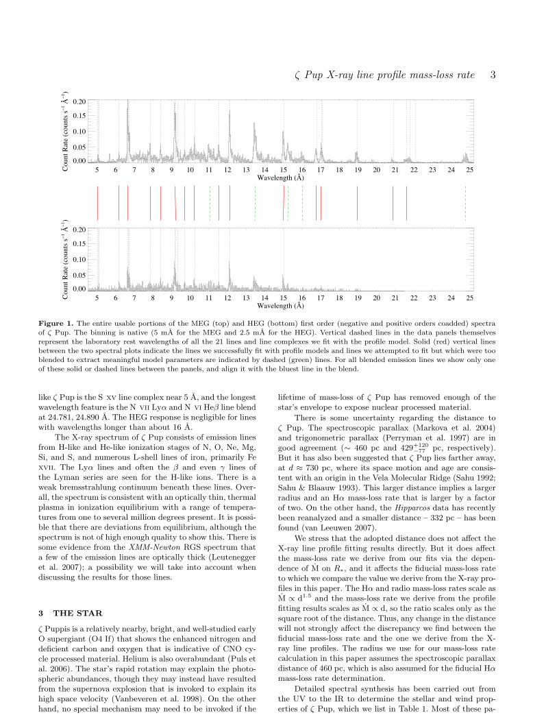
Figure 1. The entire usable portions of the MEG (top) and HEG (bottom) first order (negative and positive orders coadded) spectra

of ζ Pup. The binning is native (5 mA for the MEG and 2.5 mA for the HEG). Vertical dashed lines in the data panels themselvesrepresent the laboratory rest wavelengths of all the 21 lines and line complexes we fit with the profile model. Solid (red) vertical linesbetween the two spectral plots indicate the lines we successfully fit with profile models and lines we attempted to fit but which were tooblended to extract meaningful model parameters are indicated by dashed (green) lines. For all blended emission lines we show only one

of these solid or dashed lines between the panels, and align it with the bluest line in the blend.

like ζ Pup is the S xv line complex near 5 A, and the longestwavelength feature is the N vii Lyα and N vi Heβ line blendat 24.781, 24.890 A. The HEG response is negligible for lineswith wavelengths longer than about 16 A.

The X-ray spectrum of ζ Pup consists of emission linesfrom H-like and He-like ionization stages of N, O, Ne, Mg,Si, and S, and numerous L-shell lines of iron, primarily Fexvii. The Lyα lines and often the β and even γ lines ofthe Lyman series are seen for the H-like ions. There is aweak bremsstrahlung continuum beneath these lines. Over-all, the spectrum is consistent with an optically thin, thermalplasma in ionization equilibrium with a range of tempera-tures from one to several million degrees present. It is possi-ble that there are deviations from equilibrium, although thespectrum is not of high enough quality to show this. There issome evidence from the XMM-Newton RGS spectrum thata few of the emission lines are optically thick (Leuteneggeret al. 2007); a possibility we will take into account whendiscussing the results for those lines.

3 THE STAR

ζ Puppis is a relatively nearby, bright, and well-studied earlyO supergiant (O4 If) that shows the enhanced nitrogen anddeficient carbon and oxygen that is indicative of CNO cy-cle processed material. Helium is also overabundant (Puls etal. 2006). The star’s rapid rotation may explain the photo-spheric abundances, though they may instead have resultedfrom the supernova explosion that is invoked to explain itshigh space velocity (Vanbeveren et al. 1998). On the otherhand, no special mechanism may need to be invoked if the

lifetime of mass-loss of ζ Pup has removed enough of thestar’s envelope to expose nuclear processed material.

There is some uncertainty regarding the distance toζ Pup. The spectroscopic parallax (Markova et al. 2004)and trigonometric parallax (Perryman et al. 1997) are ingood agreement (∼ 460 pc and 429+120

−77 pc, respectively).But it has also been suggested that ζ Pup lies farther away,at d ≈ 730 pc, where its space motion and age are consis-tent with an origin in the Vela Molecular Ridge (Sahu 1992;Sahu & Blaauw 1993). This larger distance implies a largerradius and an Hα mass-loss rate that is larger by a factorof two. On the other hand, the Hipparcos data has recentlybeen reanalyzed and a smaller distance – 332 pc – has beenfound (van Leeuwen 2007).

We stress that the adopted distance does not affect theX-ray line profile fitting results directly. But it does affectthe mass-loss rate we derive from our fits via the depen-dence of M on R∗, and it affects the fiducial mass-loss rateto which we compare the value we derive from the X-ray pro-files in this paper. The Hα and radio mass-loss rates scale asM ∝ d1.5 and the mass-loss rate we derive from the profilefitting results scales as M ∝ d, so the ratio scales only as thesquare root of the distance. Thus, any change in the distancewill not strongly affect the discrepancy we find between thefiducial mass-loss rate and the one we derive from the X-ray line profiles. The radius we use for our mass-loss ratecalculation in this paper assumes the spectroscopic parallaxdistance of 460 pc, which is also assumed for the fiducial Hαmass-loss rate determination.

Detailed spectral synthesis has been carried out fromthe UV to the IR to determine the stellar and wind prop-erties of ζ Pup, which we list in Table 1. Most of these pa-

c© 0000 RAS, MNRAS 000, 000–000

4 D. Cohen et al.

Table 1. Stellar and wind parameters adopted from Puls et

al. (2006)

parameter value

Distance 460 pc

Massa 53.9 M¯Teff 39000 K

R∗ 18.6 R¯

vrotsinib 230 km s−1

v∞ 2250 km s−1

β 0.9

Mc 8.3 × 10−6 M¯ yr−1

Md 4.2 × 10−6 M¯ yr−1

a From Repolust et al. (2004).b From Glebocki et al. (2000).c Unclumped value from Puls et al. (2006).d Also from Puls et al. (2006), but the minimum clumping

model, in which the far wind, where the radio emission arises,is unclumped, but the inner wind, where the Hα is produced is

clumped. Note that the methodology of Puls et al. (2006) onlyenables a determination to be made of the relative clumpingin different regions of the wind. This value of the mass-lossrate, therefore, represents an upper limit.

rameters are taken from Puls et al. (2006). There is a rangeof wind property determinations in the extensive literatureon ζ Pup. The terminal velocity of the wind may be as lowas 2200 km s−1 (Lamers & Leitherer 1993), and as high as2485 km s−1 (Prinja et al. 1990), though we adopt the de-termination by the Munich group (Puls et al. 2006), of 2250km s−1, as our standard.

Mass-loss rate determinations vary as well. This ispartly because of the uncertainty in the distance to ζ Pup.But, it is also the case that each mass-loss rate diagnostic issubject to uncertainty: density-squared diagnostics like Hαand free-free emission are affected by clumping, no matterthe size scale or optical depth of the clumps. Mass-loss ratesfrom UV absorption lines are subject to uncertain ionizationcorrections. In the last few years there have been attemptsto account for clumping when deriving mass-loss rates fromboth density-squared diagnostics and UV absorption diag-nostics. We list two recent Hα mass-loss rate determina-tions in the table, one that assumes a smooth wind and onethat parameterizes small-scale clumping using a filling fac-tor approach. The X-ray line profile diagnostics of mass-lossrate that we employ in this paper are not directly affectedby clumping; although very large scale porosity (associatedwith optically thick clumps) can affect the profiles, as wehave already discussed.

The star shows periodic variability in various UV windlines (Howarth et al. 1995) as well as Hα (Berghoefer et al.1996). Its broad-band X-ray properties are normal for an Ostar, with Lx ≈ 10−7LBol and a soft spectrum (Hillier et al.1993), dominated by optically thin thermal line and free-freeemission from plasma with a temperature of a few milliondegrees. The emission measure filling factor of the wind issmall, roughly one part in 103. Weak soft X-ray variability,with an amplitude of 6 percent, and a period of 16.7 hr,was detected with ROSAT (Berghoefer et al. 1996). Thislow-level variability appears not to affect the Chandra data.

4 EMISSION LINE PROFILE MODEL

FITTING

4.1 The Model

The X-ray emission line profile model we fit to each linewas first described by Owocki & Cohen (2001), building onwork by MacFarlane et al. (1991) and Ignace (2001). It isa simple, spherically symmetric model that assumes the lo-cal emission scales as the ambient density squared and thatthe many sites of hot, X-ray emitting plasma are smoothlydistributed throughout the wind above some onset radius,Ro, which is expected to be several tenths of a stellar ra-dius above the photosphere in the line-driven instability sce-nario (Owocki et al. 1988; Feldmeier et al. 1997; Runacres& Owocki 2002). Attenuation of the emitted X-rays occursin the bulk, cool (T ≈ Teff) wind component via photoelec-tric absorption, mainly out of the inner shell of elementsN through Si and also out of the L-shell (n = 2) of Fe.Singly ionized helium can also make a contribution at longwavelengths. We assume that the atomic opacity of the coolwind, while a function of wavelength, does not vary signifi-cantly with radius. This is confirmed by our non-LTE windionization modelling, discussed in §5.1. We further assume abeta-velocity law, v = v∞(1−R∗/r)β , for both wind compo-nents, with v∞ = 2250 km s−1 as given by UV observations(Puls et al. 2006). The local velocity controls the wavelengthdependence of the emissivity, the local optical depth governsthe wavelength-dependent attenuation, and the density af-fects the overall level of emission. The first two of theseeffects can be visualized in Fig. 2.

We cast the expression for the line profile first in spher-ical coordinates, but evaluate some of the quantities explic-itly in terms of ray coordinates, with the origin at the centerof the star and the observer at z = ∞. We integrate the spe-cific intensity along rays of given impact parameter, p, andthen integrate over rays. Integrating over the volume of thewind, we have:

Lλ = 8π2

∫ +1

−1

dµ

∫

∞

Ro

η(µ, r)r2e−τ(µ,r)dr, (1)

where Lλ is the luminosity per unit wavelength – it is theX-ray line profile. The angular coordinate µ ≡ cos θ, andη is the wavelength-dependent emissivity that accounts forthe Doppler shift of the emitting parcel of wind material(which is completely determined, under the assumptions ofspherical symmetry and the velocity law, according to itslocation, (µ, r) or (p, z)). The emissivity has an additionalradial dependence due to the fact that it is proportionalto the square of the ambient plasma density. The opticaldepth, τ , is computed along a ray, z = µr, for each value ofthe impact parameter, p =

√

1 − µ2r, as

τ(µ, r) = t(p, z) =

∫

∞

z

κρ(r′)dz′, (2)

where the dummy radial coordinate is given by r′ ≡√

z′2 + p′2. The opacity, κ, does not vary significantly acrossa line (recall it is due to continuum processes – the strongwavelength dependence across a line profile arises purelyfrom the geometry indicated in Fig. 2). Using the continuityequation and the beta-velocity law of the wind, we have:

c© 0000 RAS, MNRAS 000, 000–000

ζ Pup X-ray line profile mass-loss rate 5

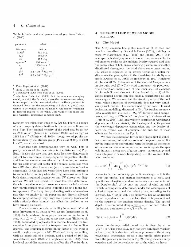
Figure 2. A visualization of the wind Doppler shift and op-

tical depth – two effects that govern the observed, broadenedand asymmetric line shapes. The observer is on the left, and thelight contours represent the line-of-sight velocity in increments of0.2v∞, with the blue shifts arising in the left hemisphere and the

red shifts in the right. The star is the gray circle at the center,and the inner radius of the wind X-ray emission, Ro, is indicated

at 1.5 R∗ by the solid black circle. The solid heavy contour rep-resents the locus of points with optical depth τ = 0.33, and thedashed and dotted contours represent τ = 1 and 3, respectively.

The model parameters visualized here are nearly identical to thoseof the best-fitting model for the Ne x Lyα line shown in Fig. 8 –Ro = 1.5; τ∗ = 2.

t(p, z) = τ∗

∫

∞

z

R∗dz′

r′2(1 − R∗/r′)β. (3)

We account for occultation of the back of the wind bythe star by setting this optical depth integral to ∞ when

p < R∗ and z <√

R∗2 − p2. The constant at the front of

eq. 3, τ∗ ≡ κM/4πR∗v∞, is the fiducial optical depth andis equivalent to the optical depth value along the centralray, integrated down to the stellar surface, in the case wherev = v∞. This quantity, τ∗, is the key parameter that de-scribes the X-ray attenuation and governs the shifted andasymmetric form of the line profiles.

We note that the optical depth integral, while generallyrequiring numerical integration, can be done analytically forinteger values of β. We use β = 1 throughout this paper(though we report on tests we did for non-integer β values in§4.3), and for that value of the parameter, the optical depthintegral along a ray with impact parameter, p, is given by:

t(p > R∗, z) =R∗τ∗

zt

(

arctanR∗

zt

+π

2

− arctanR∗µ

zt

− arctanz

zt

)

, (4)

t(p < R∗, z) =R∗τ∗2z∗

log

(

R∗ − z∗R∗ + z∗

R∗µ + z∗R∗µ − z∗

z + z∗z − z∗

)

, (5)

where zt ≡√

p2 − R∗2 and z∗ ≡

√

R∗2 − p2, and the inte-

gral has been evaluated at z and ∞.The intrinsic line profile function we assume for the

emissivity at each location is a delta function that picksout the Doppler shift line resonance,

η ∝ δ{λ − λo[1 − µv(r)/c]}. (6)

This assumption is justified because the intrinsic line widthis dominated by thermal broadening, which is very smallcompared to the Doppler shift caused by the highly super-sonic wind flow.

Calculating a line profile model, then, amounts to solv-ing equations 1 and 3 for a given set of parameters: Ro,τ∗, the normalization (which determines the overall level ofη), and an assumed wind velocity law, described by β andv∞. This last parameter, v∞, influences the emissivity termthrough its effect on the Doppler shift as a function of radiusand spherical polar angle. And for our choice of β = 1, eqs.4 and 5 replace eq. 3.

The model produces broad emission lines where theoverall width (in the sense of the second moment of the pro-file), for an assumed wind velocity law, is governed primarilyby the parameter Ro. The closer to the star’s surface Ro is,the more emission there is from low-velocity wind material,which contributes to the line profile only near line center.The value of τ∗ affects the line’s blue shift and asymmetry.The higher its value, the more blue shifted and asymmetricthe profile. Large values of τ∗ also reduce the profile widthby dramatically attenuating the red-shifted emission com-ponent of the line. The interplay of the two parameters canbe seen in fig. 2 of Owocki & Cohen (2001).

4.2 Fitting the data

4.2.1 statistical fitting of individual lines

For each line in the spectrum, our goal is to extract valuesfor the two parameters of interest – τ∗ and Ro – and to placeformal confidence limits on these values. We begin the anal-ysis procedure for each line by fitting the weak continuumsimultaneously in two regions, one to the blue side of theline and one on the red side (but excluding the wavelengthrange of the line itself). We assume the continuum is flatover this restricted wavelength region. We then fit the emis-sion line over a wavelength range that is no broader than theline itself (and sometimes even narrower, due to blends withnearby lines, which can induce us to exclude contaminatedportions of the line in question). The model we fit to eachline is the sum of the empirical line profile model – describedby equations 1, 4, and 5 – and the continuum model deter-mined from the fit to the two spectral regions near the line.Note that the inclusion of the continuum does not introduceany new free parameters. The overall model thus has onlythree free parameters: the fiducial optical depth, τ∗, the min-imum radius of X-ray emission, Ro, and the normalizationof the line. In some cases, where lines are blended, we fitmore than one profile model simultaneously, as we describebelow, but we generally keep the two main parameters ofeach profile model tied together, and so the only new freeparameter introduced is an additional line normalization.

We fit the wind profile plus continuum model to boththe MEG and HEG data (positive and negative first or-

c© 0000 RAS, MNRAS 000, 000–000

6 D. Cohen et al.

ders) simultaneously, if the HEG data are of good enoughquality to warrant their inclusion, and to the MEG dataonly if they are not. We use the C statistic (Cash 1979) asthe goodness-of-fit statistic. This is the maximum likelihoodstatistic for data with Poisson distributed errors, which thesephoton-counting X-ray spectra are. Note that the maximumlikelihood statistic for Gaussian distributed data is the well-known χ2 statistic, but it is not valid for these data, whichhave many bins with only a few counts, especially in thediagnostically powerful wings of the profiles.

We determine the best-fitting model by minimization ofthe C statistic using the fit task in xspec. Once the best-fitting model is found, the uncertainties on each model pa-rameter are assessed using the ∆χ2 formalism1 outlined inchapter 15 of Press et al. (2007), which is also valid for ∆C.We test each parameter one at a time, stepping through agrid of values and, at each step, refit the data while lettingthe other model parameters be free to vary. The 68 per-cent confidence limits determined in this manner are whatwe report as the formal uncertainties in the table of fittingresults, below. We also examine the confidence regions intwo-dimensional sub-spaces of the whole parameter spacein order to look for correlations among the interesting pa-rameters. Note that we include an extensive discussion ofmodelling uncertainties in §4.3.

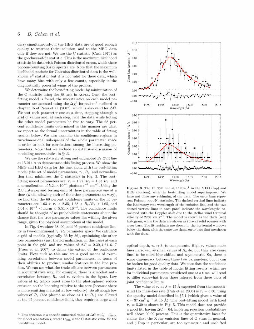
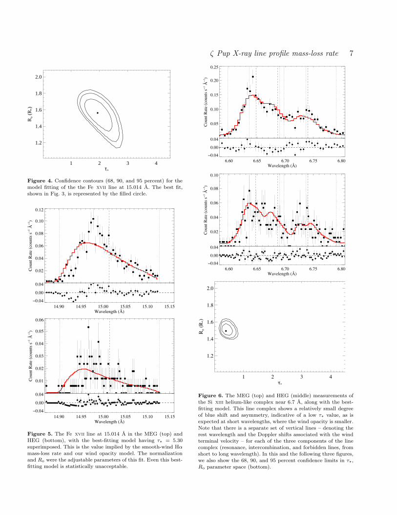
We use the relatively strong and unblended Fe xvii lineat 15.014 A to demonstrate this fitting process. We show theMEG and HEG data for this line, along with the best-fittingmodel (the set of model parameters, τ∗, Ro, and normaliza-tion that minimizes the C statistic) in Fig. 3. The best-fitting model parameters are: τ∗ = 1.97, Ro = 1.53 R∗, anda normalization of 5.24×10−4 photons s−1 cm−2. Using the∆C criterion and testing each of these parameters one at atime (while allowing each of the other parameters to vary),we find that the 68 percent confidence limits on the fit pa-rameters are 1.63 < τ∗ < 2.35, 1.38 < Ro/R∗ < 1.65, and5.04 × 10−4 < norm < 5.51 × 10−4. The confidence limitsshould be thought of as probabilistic statements about thechance that the true parameter values lies withing the givenrange, given the physical assumptions of the model.

In Fig. 4 we show 68, 90, and 95 percent confidence lim-its in two-dimensional τ∗, Ro parameter space. We calculatea grid of models (typically 36 by 36), optimizing the otherfree parameters (just the normalization, in this case) at eachpoint in the grid, and use values of ∆C = 2.30, 4.61, 6.17(Press et al. 2007) to define the extent of the confidencelimits. Plots such as this one are a good means of exam-ining correlations between model parameters, in terms oftheir abilities to produce similar features in the line pro-files. We can see what the trade offs are between parametersin a quantitative way. For example, there is a modest anti-correlation between Ro and τ∗ evident in the figure. Lowvalues of Ro (shock onset close to the photosphere) reduceemission on the line wing relative to the core (because thereis more emitting material at low velocity). So although lowvalues of Ro (hot plasma as close as 1.15 R∗) are allowedat the 95 percent confidence limit, they require a large wind

1 This criterion is a specific numerical value of ∆C ≡ Ci −Cmin

for model realization i, where Cmin is the C statistic value for the

best-fitting model.

Figure 3. The Fe xvii line at 15.014 A in the MEG (top) andHEG (bottom), with the best-fitting model superimposed. Wehave not done any rebinning of the data. The error bars repre-

sent Poisson, root-N, statistics. The dashed vertical lines indicatethe laboratory rest wavelength of the emission line, and the two

dotted vertical lines in each panel indicate the wavelengths as-

sociated with the Doppler shift due to the stellar wind terminal

velocity of 2250 km s−1. The model is shown as the thick (red)histogram, while the data are shown as (black) solid squares with

error bars. The fit residuals are shown in the horizontal windowsbelow the data, with the same one sigma error bars that are shown

with the data.

optical depth, τ∗ ≈ 3, to compensate. High τ∗ values makelines narrower, as small values of Ro do, but they also causelines to be more blue-shifted and asymmetric. So, there issome degeneracy between these two parameters, but it canbe broken for good quality data. We note that the confidencelimits listed in the table of model fitting results, which arefor individual parameters considered one at a time, will tendto differ somewhat from those inferred from these plots ofjoint confidence limits.

The value of τ∗ at λ = 15 A expected from the smooth-wind Hα mass-loss rate (Puls et al. 2006) is τ∗ = 5.30, usingthe opacity model described in §5.1 (which gives a value ofκ = 37 cm2 g−1 at 15 A). The best-fitting model with fixedτ∗ = 5.30 is shown in Fig. 5. This model does not providea good fit, having ∆C = 64, implying rejection probabilitieswell above 99.99 percent. This is the quantitative basis forclaims that the X-ray emission lines of O stars in general,and ζ Pup in particular, are too symmetric and unshifted

c© 0000 RAS, MNRAS 000, 000–000

ζ Pup X-ray line profile mass-loss rate 7

1 2 3 4τ*

1.2

1.4

1.6

1.8

2.0

Ro

(R*)

Figure 4. Confidence contours (68, 90, and 95 percent) for themodel fitting of the the Fe xvii line at 15.014 A. The best fit,shown in Fig. 3, is represented by the filled circle.

Figure 5. The Fe xvii line at 15.014 A in the MEG (top) and

HEG (bottom), with the best-fitting model having τ∗ = 5.30superimposed. This is the value implied by the smooth-wind Hα

mass-loss rate and our wind opacity model. The normalizationand Ro were the adjustable parameters of this fit. Even this best-

fitting model is statistically unacceptable.

Figure 6. The MEG (top) and HEG (middle) measurements of

the Si xiii helium-like complex near 6.7 A, along with the best-

fitting model. This line complex shows a relatively small degree

of blue shift and asymmetry, indicative of a low τ∗ value, as isexpected at short wavelengths, where the wind opacity is smaller.Note that there is a separate set of vertical lines – denoting the

rest wavelength and the Doppler shifts associated with the wind

terminal velocity – for each of the three components of the line

complex (resonance, intercombination, and forbidden lines, from

short to long wavelength). In this and the following three figures,we also show the 68, 90, and 95 percent confidence limits in τ∗,

Ro parameter space (bottom).

c© 0000 RAS, MNRAS 000, 000–000

8 D. Cohen et al.

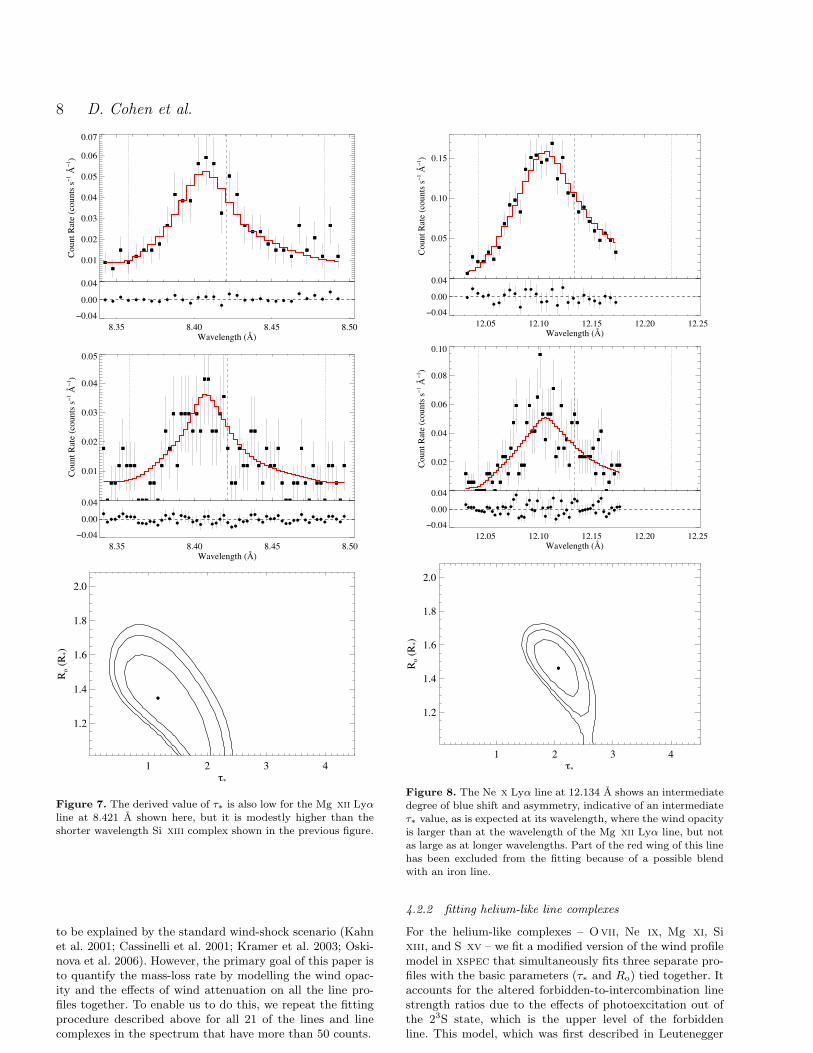
Figure 7. The derived value of τ∗ is also low for the Mg xii Lyα

line at 8.421 A shown here, but it is modestly higher than the

shorter wavelength Si xiii complex shown in the previous figure.

to be explained by the standard wind-shock scenario (Kahnet al. 2001; Cassinelli et al. 2001; Kramer et al. 2003; Oski-nova et al. 2006). However, the primary goal of this paper isto quantify the mass-loss rate by modelling the wind opac-ity and the effects of wind attenuation on all the line pro-files together. To enable us to do this, we repeat the fittingprocedure described above for all 21 of the lines and linecomplexes in the spectrum that have more than 50 counts.

Figure 8. The Ne x Lyα line at 12.134 A shows an intermediate

degree of blue shift and asymmetry, indicative of an intermediateτ∗ value, as is expected at its wavelength, where the wind opacity

is larger than at the wavelength of the Mg xii Lyα line, but notas large as at longer wavelengths. Part of the red wing of this line

has been excluded from the fitting because of a possible blend

with an iron line.

4.2.2 fitting helium-like line complexes

For the helium-like complexes – Ovii, Ne ix, Mg xi, Sixiii, and S xv – we fit a modified version of the wind profilemodel in xspec that simultaneously fits three separate pro-files with the basic parameters (τ∗ and Ro) tied together. Itaccounts for the altered forbidden-to-intercombination linestrength ratios due to the effects of photoexcitation out ofthe 23S state, which is the upper level of the forbiddenline. This model, which was first described in Leutenegger

c© 0000 RAS, MNRAS 000, 000–000

ζ Pup X-ray line profile mass-loss rate 9

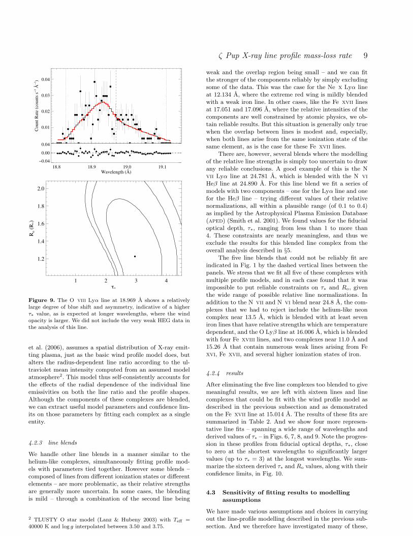
Figure 9. The O viii Lyα line at 18.969 A shows a relativelylarge degree of blue shift and asymmetry, indicative of a higher

τ∗ value, as is expected at longer wavelengths, where the windopacity is larger. We did not include the very weak HEG data inthe analysis of this line.

et al. (2006), assumes a spatial distribution of X-ray emit-ting plasma, just as the basic wind profile model does, butalters the radius-dependent line ratio according to the ul-traviolet mean intensity computed from an assumed modelatmosphere2. This model thus self-consistently accounts forthe effects of the radial dependence of the individual lineemissivities on both the line ratio and the profile shapes.Although the components of these complexes are blended,we can extract useful model parameters and confidence lim-its on those parameters by fitting each complex as a singleentity.

4.2.3 line blends

We handle other line blends in a manner similar to thehelium-like complexes, simultaneously fitting profile mod-els with parameters tied together. However some blends –composed of lines from different ionization states or differentelements – are more problematic, as their relative strengthsare generally more uncertain. In some cases, the blendingis mild – through a combination of the second line being

2 TLUSTY O star model (Lanz & Hubeny 2003) with Teff =

40000 K and log g interpolated between 3.50 and 3.75.

weak and the overlap region being small – and we can fitthe stronger of the components reliably by simply excludingsome of the data. This was the case for the Ne x Lyα lineat 12.134 A, where the extreme red wing is mildly blendedwith a weak iron line. In other cases, like the Fe xvii linesat 17.051 and 17.096 A, where the relative intensities of thecomponents are well constrained by atomic physics, we ob-tain reliable results. But this situation is generally only truewhen the overlap between lines is modest and, especially,when both lines arise from the same ionization state of thesame element, as is the case for these Fe xvii lines.

There are, however, several blends where the modellingof the relative line strengths is simply too uncertain to drawany reliable conclusions. A good example of this is the Nvii Lyα line at 24.781 A, which is blended with the N vi

Heβ line at 24.890 A. For this line blend we fit a series ofmodels with two components – one for the Lyα line and onefor the Heβ line – trying different values of their relativenormalizations, all within a plausible range (of 0.1 to 0.4)as implied by the Astrophysical Plasma Emission Database(aped) (Smith et al. 2001). We found values for the fiducialoptical depth, τ∗, ranging from less than 1 to more than4. These constraints are nearly meaningless, and thus weexclude the results for this blended line complex from theoverall analysis described in §5.

The five line blends that could not be reliably fit areindicated in Fig. 1 by the dashed vertical lines between thepanels. We stress that we fit all five of these complexes withmultiple profile models, and in each case found that it wasimpossible to put reliable constraints on τ∗ and Ro, giventhe wide range of possible relative line normalizations. Inaddition to the N vii and N vi blend near 24.8 A, the com-plexes that we had to reject include the helium-like neoncomplex near 13.5 A, which is blended with at least seveniron lines that have relative strengths which are temperaturedependent, and the O Lyβ line at 16.006 A, which is blendedwith four Fe xviii lines, and two complexes near 11.0 A and15.26 A that contain numerous weak lines arising from Fexvi, Fe xvii, and several higher ionization states of iron.

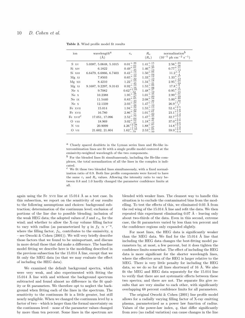
4.2.4 results

After eliminating the five line complexes too blended to givemeaningful results, we are left with sixteen lines and linecomplexes that could be fit with the wind profile model asdescribed in the previous subsection and as demonstratedon the Fe xvii line at 15.014 A. The results of these fits aresummarized in Table 2. And we show four more represen-tative line fits – spanning a wide range of wavelengths andderived values of τ∗ – in Figs. 6, 7, 8, and 9. Note the progres-sion in these profiles from fiducial optical depths, τ∗, closeto zero at the shortest wavelengths to significantly largervalues (up to τ∗ = 3) at the longest wavelengths. We sum-marize the sixteen derived τ∗ and Ro values, along with theirconfidence limits, in Fig. 10.

4.3 Sensitivity of fitting results to modelling

assumptions

We have made various assumptions and choices in carryingout the line-profile modelling described in the previous sub-section. And we therefore have investigated many of these,

c© 0000 RAS, MNRAS 000, 000–000

10 D. Cohen et al.

Table 2. Wind profile model fit results

ion wavelengtha τ∗ Ro normalizationb

(A) (R∗) (10−5 ph cm−2 s−1)

S xv 5.0387, 5.0648, 5.1015 0.01+.36−.01 1.41+.15

−.11 2.56+.24−.36

Si xiv 6.1822 0.49+.61−.35 1.46+.20

−.14 0.77+.11−.14

Si xiii 6.6479, 6.6866, 6.7403 0.42+.14−.13 1.50+.06

−.04 11.2+.4−.4

Mg xi 7.8503 0.65+.19−.32 1.33+.12

−.13 1.33+.17−.13

Mg xii 8.4210 1.22+.53−.45 1.34+.18

−.21 2.95+.24−.24

Mg xi 9.1687, 9.2297, 9.3143 0.92+.19−.16 1.55+.06

−.06 17.8+.8−.5

Ne x 9.7082 0.62+1.05−.52 1.48+.27

−.19 0.95+.15−.15

Ne x 10.2388 1.95+.28−.87 1.01+.45

−.00 2.99+.31−.29

Ne ix 11.5440 0.83+.65−.44 2.08+.54

−.36 5.00+.40−.50

Ne x 12.1339 2.03+.24−.28 1.47+.11

−.10 26.9+1.1−.7

Fe xvii 15.014 1.94+.32−.33 1.55+.13

−.12 52.4+2.5−1.6

Fe xvii 16.780 2.86+.38−.71 1.01+.61

−.00 23.1+1.9−1.2

Fe xviic 17.051, 17.096 2.52+.70

−.64 1.47+.35−.46 32.7+0.9

−1.1

O viii 18.969 3.02+.52−.57 1.18+.41

−.17 37.0+2.8−2.6

N vii 20.9099 4.26+2.28−1.71 1.88+.87

−.87 14.8+2.3−1.9

O vii 21.602, 21.804 1.62+1.33−.79 2.53+.85

−.50 59.9+4.9−5.4

a Closely spaced doublets in the Lyman series lines and He-like in-tercombination lines are fit with a single profile model centered at theemissivity-weighted wavelength of the two components.b For the blended lines fit simultaneously, including the He-like com-

plexes, the total normalization of all the lines in the complex is indi-cated.c We fit these two blended lines simultaneously, with a fixed normal-ization ratio of 0.9. Both line profile components were forced to have

the same τ∗ and Ro values. Allowing the intensity ratio to vary be-tween 0.8 and 1.0 hardly changed the parameter confidence limits at

all.

again using the Fe xvii line at 15.014 A as a test case. Inthis subsection, we report on the sensitivity of our resultsto the following assumptions and choices: background sub-traction; determination of the continuum level; exclusion ofportions of the line due to possible blending; inclusion ofthe weak HEG data; the adopted values of β and v∞ for thewind; and whether to allow the X-ray volume filling factorto vary with radius (as parameterized by q in fX ∝ r−q,where the filling factor, fX, contributes to the emissivity, η– see Owocki & Cohen (2001)). We will very briefly describethose factors that we found to be unimportant, and discussin more detail those that did make a difference. The baselinemodel fitting we describe here is the modelling described inthe previous subsection for the 15.014 A line, except that wefit only the MEG data (so that we may evaluate the effectof including the HEG data).

We examined the default background spectra, whichwere very weak, and also experimented with fitting the15.014 A line with and without the background spectrumsubtracted and found almost no difference in the fit qual-ity or fit parameters. We therefore opt to neglect the back-ground when fitting each of the lines in the spectrum. Thesensitivity to the continuum fit is a little greater, but stillnearly negligible. When we changed the continuum level by afactor of two – which is larger than the formal uncertainty onthe continuum level – none of the parameter values changedby more than ten percent. Some lines in the spectrum are

blended with weaker lines. The cleanest way to handle thissituation is to exclude the contaminated bins from the mod-elling. To test the effects of this, we eliminated 0.03 A fromthe red wing of the 15.014 A line and refit the data. We thenrepeated this experiment eliminating 0.07 A - leaving onlyabout two-thirds of the data. Even in this second, extremecase, the fit parameters varied by less than ten percent andthe confidence regions only expanded slightly.

For most lines, the HEG data is significantly weakerthan the MEG data. We find for the 15.014 A line thatincluding the HEG data changes the best-fitting model pa-rameters by, at most, a few percent, but it does tighten theconfidence limits somewhat. The effect of including the HEGdata is more significant for the shorter wavelength lines,where the effective area of the HEG is larger relative to theMEG. There is very little penalty for including the HEGdata, so we do so for all lines shortward of 16 A. We alsofit the MEG and HEG data separately for the 15.014 lineto verify that there are not systematic effects between thesetwo spectra; and there are not. The separate fits give re-sults that are very similar to each other, with significantlyoverlapping 68 percent confidence limits for all parameters.

The original Owocki & Cohen (2001) line profile modelallows for a radially varying filling factor of X-ray emittingplasma, parameterized as a power law function of radius.Values of the power-law index, q, that differ significantlyfrom zero (no radial variation) can cause changes in the line

c© 0000 RAS, MNRAS 000, 000–000

ζ Pup X-ray line profile mass-loss rate 11

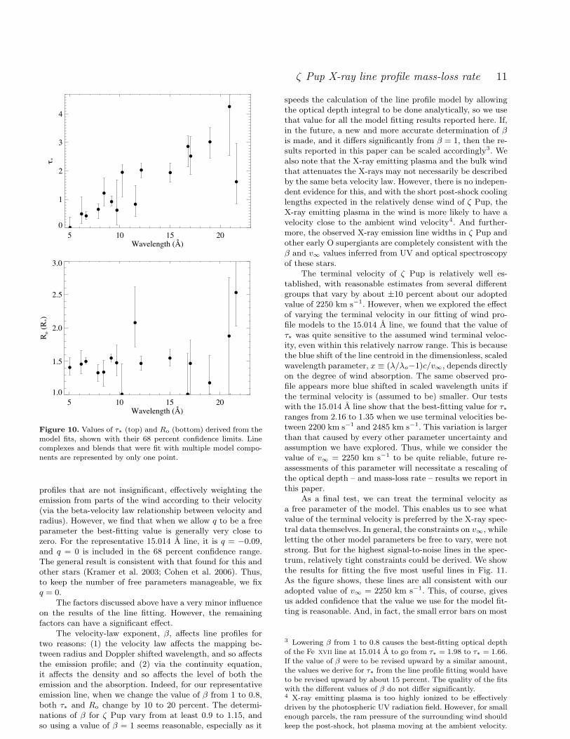
Figure 10. Values of τ∗ (top) and Ro (bottom) derived from themodel fits, shown with their 68 percent confidence limits. Line

complexes and blends that were fit with multiple model compo-nents are represented by only one point.

profiles that are not insignificant, effectively weighting theemission from parts of the wind according to their velocity(via the beta-velocity law relationship between velocity andradius). However, we find that when we allow q to be a freeparameter the best-fitting value is generally very close tozero. For the representative 15.014 A line, it is q = −0.09,and q = 0 is included in the 68 percent confidence range.The general result is consistent with that found for this andother stars (Kramer et al. 2003; Cohen et al. 2006). Thus,to keep the number of free parameters manageable, we fixq = 0.

The factors discussed above have a very minor influenceon the results of the line fitting. However, the remainingfactors can have a significant effect.

The velocity-law exponent, β, affects line profiles fortwo reasons: (1) the velocity law affects the mapping be-tween radius and Doppler shifted wavelength, and so affectsthe emission profile; and (2) via the continuity equation,it affects the density and so affects the level of both theemission and the absorption. Indeed, for our representativeemission line, when we change the value of β from 1 to 0.8,both τ∗ and Ro change by 10 to 20 percent. The determi-nations of β for ζ Pup vary from at least 0.9 to 1.15, andso using a value of β = 1 seems reasonable, especially as it

speeds the calculation of the line profile model by allowingthe optical depth integral to be done analytically, so we usethat value for all the model fitting results reported here. If,in the future, a new and more accurate determination of βis made, and it differs significantly from β = 1, then the re-sults reported in this paper can be scaled accordingly3. Wealso note that the X-ray emitting plasma and the bulk windthat attenuates the X-rays may not necessarily be describedby the same beta velocity law. However, there is no indepen-dent evidence for this, and with the short post-shock coolinglengths expected in the relatively dense wind of ζ Pup, theX-ray emitting plasma in the wind is more likely to have avelocity close to the ambient wind velocity4. And further-more, the observed X-ray emission line widths in ζ Pup andother early O supergiants are completely consistent with theβ and v∞ values inferred from UV and optical spectroscopyof these stars.

The terminal velocity of ζ Pup is relatively well es-tablished, with reasonable estimates from several differentgroups that vary by about ±10 percent about our adoptedvalue of 2250 km s−1. However, when we explored the effectof varying the terminal velocity in our fitting of wind pro-file models to the 15.014 A line, we found that the value ofτ∗ was quite sensitive to the assumed wind terminal veloc-ity, even within this relatively narrow range. This is becausethe blue shift of the line centroid in the dimensionless, scaledwavelength parameter, x ≡ (λ/λo−1)c/v∞, depends directlyon the degree of wind absorption. The same observed pro-file appears more blue shifted in scaled wavelength units ifthe terminal velocity is (assumed to be) smaller. Our testswith the 15.014 A line show that the best-fitting value for τ∗ranges from 2.16 to 1.35 when we use terminal velocities be-tween 2200 km s−1 and 2485 km s−1. This variation is largerthan that caused by every other parameter uncertainty andassumption we have explored. Thus, while we consider thevalue of v∞ = 2250 km s−1 to be quite reliable, future re-assessments of this parameter will necessitate a rescaling ofthe optical depth – and mass-loss rate – results we report inthis paper.

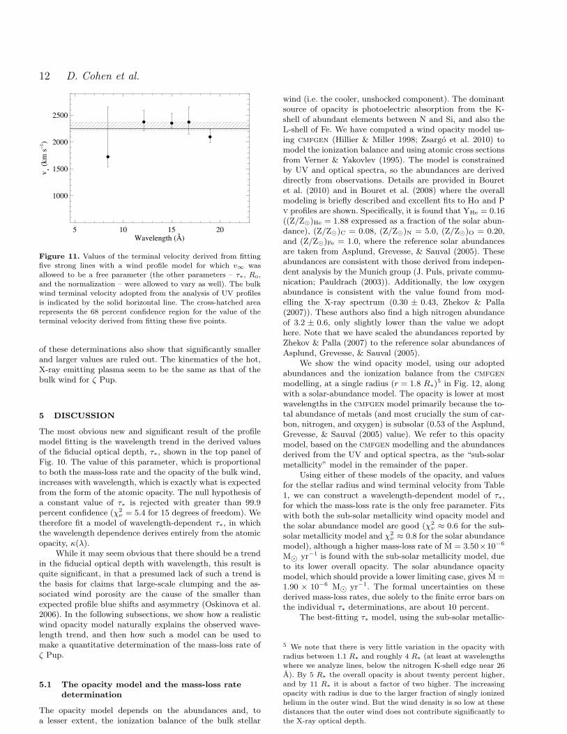
As a final test, we can treat the terminal velocity asa free parameter of the model. This enables us to see whatvalue of the terminal velocity is preferred by the X-ray spec-tral data themselves. In general, the constraints on v∞, whileletting the other model parameters be free to vary, were notstrong. But for the highest signal-to-noise lines in the spec-trum, relatively tight constraints could be derived. We showthe results for fitting the five most useful lines in Fig. 11.As the figure shows, these lines are all consistent with ouradopted value of v∞ = 2250 km s−1. This, of course, givesus added confidence that the value we use for the model fit-ting is reasonable. And, in fact, the small error bars on most

3 Lowering β from 1 to 0.8 causes the best-fitting optical depthof the Fe xvii line at 15.014 A to go from τ∗ = 1.98 to τ∗ = 1.66.

If the value of β were to be revised upward by a similar amount,the values we derive for τ∗ from the line profile fitting would have

to be revised upward by about 15 percent. The quality of the fits

with the different values of β do not differ significantly.4 X-ray emitting plasma is too highly ionized to be effectively

driven by the photospheric UV radiation field. However, for small

enough parcels, the ram pressure of the surrounding wind shouldkeep the post-shock, hot plasma moving at the ambient velocity.

c© 0000 RAS, MNRAS 000, 000–000

12 D. Cohen et al.

Figure 11. Values of the terminal velocity derived from fittingfive strong lines with a wind profile model for which v∞ wasallowed to be a free parameter (the other parameters – τ∗, Ro,and the normalization – were allowed to vary as well). The bulkwind terminal velocity adopted from the analysis of UV profiles

is indicated by the solid horizontal line. The cross-hatched arearepresents the 68 percent confidence region for the value of theterminal velocity derived from fitting these five points.

of these determinations also show that significantly smallerand larger values are ruled out. The kinematics of the hot,X-ray emitting plasma seem to be the same as that of thebulk wind for ζ Pup.

5 DISCUSSION

The most obvious new and significant result of the profilemodel fitting is the wavelength trend in the derived valuesof the fiducial optical depth, τ∗, shown in the top panel ofFig. 10. The value of this parameter, which is proportionalto both the mass-loss rate and the opacity of the bulk wind,increases with wavelength, which is exactly what is expectedfrom the form of the atomic opacity. The null hypothesis ofa constant value of τ∗ is rejected with greater than 99.9percent confidence (χ2

ν = 5.4 for 15 degrees of freedom). Wetherefore fit a model of wavelength-dependent τ∗, in whichthe wavelength dependence derives entirely from the atomicopacity, κ(λ).

While it may seem obvious that there should be a trendin the fiducial optical depth with wavelength, this result isquite significant, in that a presumed lack of such a trend isthe basis for claims that large-scale clumping and the as-sociated wind porosity are the cause of the smaller thanexpected profile blue shifts and asymmetry (Oskinova et al.2006). In the following subsections, we show how a realisticwind opacity model naturally explains the observed wave-length trend, and then how such a model can be used tomake a quantitative determination of the mass-loss rate ofζ Pup.

5.1 The opacity model and the mass-loss rate

determination

The opacity model depends on the abundances and, toa lesser extent, the ionization balance of the bulk stellar

wind (i.e. the cooler, unshocked component). The dominantsource of opacity is photoelectric absorption from the K-shell of abundant elements between N and Si, and also theL-shell of Fe. We have computed a wind opacity model us-ing cmfgen (Hillier & Miller 1998; Zsargo et al. 2010) tomodel the ionization balance and using atomic cross sectionsfrom Verner & Yakovlev (1995). The model is constrainedby UV and optical spectra, so the abundances are deriveddirectly from observations. Details are provided in Bouretet al. (2010) and in Bouret et al. (2008) where the overallmodeling is briefly described and excellent fits to Hα and Pv profiles are shown. Specifically, it is found that YHe = 0.16((Z/Z¯)He = 1.88 expressed as a fraction of the solar abun-dance), (Z/Z¯)C = 0.08, (Z/Z¯)N = 5.0, (Z/Z¯)O = 0.20,and (Z/Z¯)Fe = 1.0, where the reference solar abundancesare taken from Asplund, Grevesse, & Sauval (2005). Theseabundances are consistent with those derived from indepen-dent analysis by the Munich group (J. Puls, private commu-nication; Pauldrach (2003)). Additionally, the low oxygenabundance is consistent with the value found from mod-elling the X-ray spectrum (0.30 ± 0.43, Zhekov & Palla(2007)). These authors also find a high nitrogen abundanceof 3.2 ± 0.6, only slightly lower than the value we adopthere. Note that we have scaled the abundances reported byZhekov & Palla (2007) to the reference solar abundances ofAsplund, Grevesse, & Sauval (2005).

We show the wind opacity model, using our adoptedabundances and the ionization balance from the cmfgen

modelling, at a single radius (r = 1.8 R∗)5 in Fig. 12, along

with a solar-abundance model. The opacity is lower at mostwavelengths in the cmfgen model primarily because the to-tal abundance of metals (and most crucially the sum of car-bon, nitrogen, and oxygen) is subsolar (0.53 of the Asplund,Grevesse, & Sauval (2005) value). We refer to this opacitymodel, based on the cmfgen modelling and the abundancesderived from the UV and optical spectra, as the “sub-solarmetallicity” model in the remainder of the paper.

Using either of these models of the opacity, and valuesfor the stellar radius and wind terminal velocity from Table1, we can construct a wavelength-dependent model of τ∗,for which the mass-loss rate is the only free parameter. Fitswith both the sub-solar metallicity wind opacity model andthe solar abundance model are good (χ2

ν ≈ 0.6 for the sub-solar metallicity model and χ2

ν ≈ 0.8 for the solar abundancemodel), although a higher mass-loss rate of M = 3.50×10−6

M¯ yr−1 is found with the sub-solar metallicity model, dueto its lower overall opacity. The solar abundance opacitymodel, which should provide a lower limiting case, gives M =1.90 × 10−6 M¯ yr−1. The formal uncertainties on thesederived mass-loss rates, due solely to the finite error bars onthe individual τ∗ determinations, are about 10 percent.

The best-fitting τ∗ model, using the sub-solar metallic-

5 We note that there is very little variation in the opacity with

radius between 1.1 R∗ and roughly 4 R∗ (at least at wavelengths

where we analyze lines, below the nitrogen K-shell edge near 26A). By 5 R∗ the overall opacity is about twenty percent higher,

and by 11 R∗ it is about a factor of two higher. The increasing

opacity with radius is due to the larger fraction of singly ionized

helium in the outer wind. But the wind density is so low at thesedistances that the outer wind does not contribute significantly to

the X-ray optical depth.

c© 0000 RAS, MNRAS 000, 000–000

ζ Pup X-ray line profile mass-loss rate 13

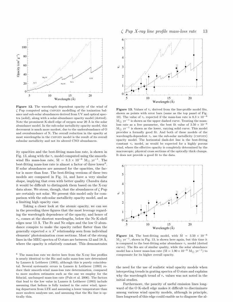
Figure 12. The wavelength dependent opacity of the wind of

ζ Pup computed using cmfgen modelling of the ionization bal-ance and sub-solar abundances derived from UV and optical spec-tra (solid), along with a solar-abundance opacity model (dotted).Note the prominent K-shell edge of oxygen near 20 A in the solarabundance model. In the sub-solar metallicity opacity model, thisdecrement is much more modest, due to the underabundance of O

and overabundance of N. The overall reduction in the opacity atmost wavelengths in the cmfgen model is the result of its overall

subsolar metallicity and not its altered CNO abundances.

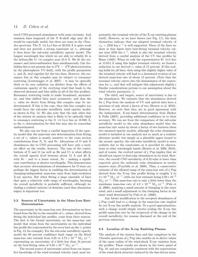
ity opacities and the best-fitting mass-loss rate, is shown inFig. 13, along with the τ∗ model computed using the smooth-wind Hα mass-loss rate, M = 8.3 × 10−6 M¯ yr−1. Thebest-fitting mass-loss rate is almost a factor of three lower6.If solar abundances are assumed for the opacities, the fac-tor is more than four. The best-fitting versions of these twomodels are compared in Fig. 14, and have a very similarshape, implying that even with better quality Chandra datait would be difficult to distinguish them based on the X-raydata alone. We stress, though, that the abundances of ζ Pupare certainly not solar. We present this model only for com-parison with the sub-solar metallicity opacity model, and asa limiting high opacity case.

Taking a closer look at the atomic opacity, we can seein the preceding three figures that the most leverage regard-ing the wavelength dependence of the opacity, and hence ofτ∗, comes at the shortest wavelengths, below the Ne K-shelledges near 13 A. The Fe and Ne edges and the low O abun-dance conspire to make the opacity rather flatter than thegenerally expected κ ∝ λ3 relationship seen from individualelements’ photoionization cross sections. Most of the stronglines in the MEG spectra of O stars are between 12 and 18 A,where the opacity is relatively constant. This demonstrates

6 The mass-loss rate we derive here from the X-ray line profiles

is nearly identical to the Hα and radio mass-loss rate determined

by Lamers & Leitherer (1993), although this is purely coinciden-

tal. Several systematic errors in Lamers & Leitherer (1993) re-

duce their smooth-wind mass-loss rate determination, compared

to more modern estimates such as the one we employ for thefiducial, unclumped mass-loss rate (Puls et al. 2006). The factors

that lead to the low value in Lamers & Leitherer (1993) include

assuming that helium is fully ionized in the outer wind, ignor-

ing departures from LTE and assuming a lower temperature thanmore modern analyses use, and assuming that the Hα line is op-

tically thin.

Figure 13. Values of τ∗ derived from the line-profile model fits,shown as points with error bars (same as the top panel of Fig.

10). The value of τ∗ expected if the mass-loss rate is 8.3 × 10−6

M¯ yr−1 is shown as the upper dashed curve. Treating the mass-loss rate as a free parameter, the best fit value of 3.50 × 10−6

M¯ yr−1 is shown as the lower, varying solid curve. This modelprovides a formally good fit. And both of these models of thewavelength-dependent τ∗ use the sub-solar metallicity (cmfgen)opacity model. The horizontal dash-dot line is the best-fitting

constant τ∗ model, as would be expected for a highly porouswind, where the effective opacity is completely determined by themacroscopic, physical cross sections of the optically thick clumps.

It does not provide a good fit to the data.

Figure 14. The best-fitting model, with M = 3.50 × 10−6

M¯ yr−1, shown in Fig. 13, is shown here again, but this time itis compared to the best-fitting solar abundance τ∗ model (dotted

curve). The fits are of similar quality, while the solar abundancemodel has a lower mass-loss rate (M = 1.90× 10−6 M¯ yr−1) to

compensate for its higher overall opacity.

the need for the use of realistic wind opacity models wheninterpreting trends in grating spectra of O stars and explainswhy the wavelength trend of τ∗ values was not noted in theinitial studies.

Furthermore, the paucity of useful emission lines long-ward of the O K-shell edge makes it difficult to discriminateamong various wind opacity models, although in principle,lines longward of this edge could enable us to diagnose the al-

c© 0000 RAS, MNRAS 000, 000–000

14 D. Cohen et al.

tered CNO-processed abundances with some certainty. Andemission lines longward of the N K-shell edge near 26 Awould be especially useful, but there are none in the Chan-

dra spectrum. The N vii Lyβ line at 20.910 A is quite weakand does not provide a strong constraint on τ∗, althoughit does favor the sub-solar metallicity opacity model. Thelongest wavelength line which we are able to reliably fit isthe helium-like O vii complex near 21.8 A. We fit the res-onance and intercombination lines simultaneously (the for-bidden line is not present due to 23S − 23P photoexcitationby the photospheric UV field), with the profile parametersτ∗ and Ro tied together for the two lines. However, the res-onance line in this complex may be subject to resonancescattering (Leutenegger et al. 2007) – it may be opticallythick to its own radiation (as distinct from the effects ofcontinuum opacity of the overlying wind that leads to theobserved skewness and blue shifts in all of the line profiles).Resonance scattering tends to make broadened, asymmet-ric, and blue shifted lines more symmetric, and thus theτ∗ value we derive from fitting this complex may be un-derestimated. If this is the case, then this line complex toowould favor the sub-solar metallicity wind opacity model,as shown in Fig. 14. We also note that the only other lineof the sixteen we analyze that is likely to be optically thickto resonance scattering is the O vii Lyα line at 18.969 A,so the τ∗ determination for that line may also be somewhatunderestimated.

We also can see from a careful inspection of the opac-ity model that the mass-loss rate determination from fittinga set of τ∗ values is mostly sensitive to the cross sectioncontributions from N, O, and Fe. Alterations of O and Nabundances due to CNO processing will have only a mod-est effect on the results, however. The sum of the contri-butions of N and O (as well as He and C) is what affectsthe overall opacity level between about 15 A and 20 A,with Fe – and to a lesser extent, Ne – making a signifi-cant contribution at shorter wavelengths. This demonstratesthat accurate determinations of abundances for O stars areperhaps the biggest factor in enabling the determination ofclumping-independent mass-loss rates from high-resolutionX-ray spectra. But when fitting a large ensemble of linesthat span a relatively wide range of wavelengths, knowingthe overall metallicity is probably sufficient, although in-cluding a realistic mixture of elements (and thus absorptionedges) is important too.

5.2 Sources of Uncertainty in the Mass-Loss Rate

Determination

The uncertainty in the mass-loss rate determination we havefound from the fits to the ensemble of τ∗ values, derived fromfitting the individual line profiles, come from three sources.The first is the formal uncertainty on the mass-loss ratemodel that stems from the uncertainties on the individualline profile fits (represented by the error bars on the τ∗ pointsin Fig. 13, for example). For the sub-solar metallicity opacitymodel the 68 percent confidence limit range on the fittedmass-loss rate extends from 3.25 to 3.73 × 10−6 M¯ yr−1,representing an uncertainty of a little less than 10 percenton the best-fitting value of 3.50 × 10−6 M¯ yr−1.

The second source of uncertainty arises from our imper-fect knowledge of the wind terminal velocity (and, most im-

portantly, the terminal velocity of the X-ray emitting plasmaitself). However, as we have shown (see Fig. 11), the datathemselves indicate that our adopted terminal velocity ofv∞ = 2250 km s−1 is well supported. Three of the lines weshow in that figure have best-fitting terminal velocity val-ues near 2350 km s−1, which is also the terminal velocityderived from a careful analysis of the UV line profiles byHaser (1995). When we refit the representative Fe xvii lineat 15.014 A using this higher terminal velocity, we found areduction in our derived τ∗ value of 15 percent. If this scal-ing holds for all lines, then using this slightly higher value ofthe terminal velocity will lead to a downward revision of ourderived mass-loss rate of about 15 percent. (Note that theterminal velocity enters into the denominator of the expres-sion for τ∗, and that will mitigate this adjustment slightly.)Similar considerations pertain to our assumption about thewind velocity parameter, β.

The third, and largest, source of uncertainty is due tothe abundances. We estimate that the abundances derivedfor ζ Pup from the analysis of UV and optical data have aprecision of only about a factor of two (Bouret et al. 2010).However, we note that they are in good agreement withthe independent, X-ray-based determination from Zhekov& Palla (2007), providing additional confidence as to theiraccuracy. We can see from the comparison of the sub-solarmetallicity model to the solar abundance model that themass-loss rate varies by about a factor of two between thesetwo assumed opacity models, although the solar abundancemodel is included in our analysis not so much as a realisticalternate model, but simply as a plausible upper bound tothe atomic opacity; the sub-solar metallicity model is morerealistic due to the constraints on it provided by observa-tions in other wavelength bands (Bouret et al. 2008, 2010),and of course, the evolved nature of ζ Pup implies that weshould not expect to find solar abundances in its wind. How-ever, the overall CNO metallicity of 0.53 solar is lower thanexpected, given the uniformly solar abundances in nearbymassive stars (Przybilla et al. 2008). Thus, a conservativeestimate of the allowed range of the mass-loss rate of ζ Pupderived from the X-ray line profile fitting is roughly 2 to4×10−6 M¯ yr−1, with our best estimate being 3.50×10−6

M¯ yr−1. This mass-loss rate is only a little lower than themaximum mass-loss rate of 4.2 × 10−6 M¯ yr−1 (Puls etal. 2006), implying a small amount of clumping in the outerwind, and a small adjustment to the clumping factor in theinner wind determined by Puls et al. (2006).

Any future modification to the accepted abundances ofζ Pup could lead to a change in the mass-loss rate impliedby our X-ray line profile analysis. To a good approximation,such a change would simply involve scaling the X-ray lineprofile mass-loss rate by the reciprocal of the change in theoverall metallicity, for reasons discussed at the end of theprevious subsection.

5.3 Location of the X-ray Emitting Plasma

The analysis of the sixteen lines and line complexes in theChandra spectrum of ζ Pup also enables us to derive valuesof the onset radius of the wind-shock X-ray emission fromthe profiles. These results are shown in the lower panel ofFig. 10, and are completely consistent with the expectationsof the wind-shock structure induced by the line-driven insta-

c© 0000 RAS, MNRAS 000, 000–000

ζ Pup X-ray line profile mass-loss rate 15

bility (Feldmeier et al. 1997; Runacres & Owocki 2002). Thatis, an onset radius of Ro ≈ 1.5 R∗ (from a weighted fit to theresults from the sixteen fitted lines and line complexes; withan uncertainty of 0.1 R∗). We have searched for a trend withwavelength in these values and found none7. Thus, the sim-plest interpretation is that there is a universal radius of theonset of X-ray emission and it occurs near 1.5 R∗ (half a stel-lar radius above the photosphere). This result had alreadybeen noted by Kramer et al. (2003), though we show it morerobustly here. This same result can also be seen in the late Osupergiant ζ Ori (Cohen et al. 2006). And this result is alsoconsistent with the joint analysis of X-ray line profile shapesand helium-like forbidden-to-intercombination line ratios forfour O stars as described by Leutenegger et al. (2006).

5.4 Comparison with Previous Analyses

Finally, let us consider why we have found a trend in wave-length for the fiducial optical depth values, τ∗, derived fromthe same Chandra data that led Kramer et al. (2003) toreport that there was no obvious trend. The two biggestfactors leading to this new result are our more careful as-sessment of line blends, and our inclusion of many weak, butimportant, lines at short wavelength. Kramer et al. (2003)included only one line shortward of the Ne x Lyα line at12.134 A, whereas we report on nine lines or line com-plexes in this range (including two helium-like complexes,which Kramer et al. (2003) excluded from their analysis).While many of these lines are weak and do not provide verystrong constraints when considered individually, taken to-gether, they are highly statistically significant. As for lineblends, Kramer et al. (2003) included the N vii Lyα lineat 24.781 A and the Fe xvii complex near 15.26 A, both ofwhich we have determined are too blended to allow the ex-traction of reliable information about their intrinsic profileshapes. Furthermore, we properly account for the blendedFe xvii lines at 17.051 and 17.096 A, fitting them simul-taneously, while Kramer et al. (2003) fit them as a singleline.

Nonetheless, if we exclude the blended 17.05, 17.10 Alines, our τ∗ values for each line also analyzed by Krameret al. (2003) are in agreement to within the error bars. Sim-ilarly, for five unblended lines in the analysis of the samedata by Yamamoto et al. (2007), we find consistent results.In fact, the wavelength trend of τ∗ is fully consistent withthe τ∗ values found by Yamamoto et al. (2007), but therewere not enough lines in that study for the trend to be un-ambiguously detected. The seven additional lines and linecomplexes that are not analyzed in any other study (Krameret al. 2003; Leutenegger et al. 2006; Yamamoto et al. 2007)but which we analyze here are crucial for mapping out thewavelength dependence of τ∗.

An additional factor that enabled us to determine thatthe wavelength trend in τ∗ is consistent with that expectedfrom the form of the atomic opacity of the wind is our use

7 An unweighted fit of an assumed linear trend shows a modestincrease with wavelength, but that result is significant at only the

one sigma level, and when we perform a weighted fit – with the

weights inversely proportional to the uncertainties on the individ-ual measurements – the significance is less than one sigma.

of a detailed model of the wind opacity. It is relatively flatover much of the wavelength range encompassing the stronglines in the Chandra spectrum. Specifically, from about 12A to about 18 A, the presence of successive ionization edgesmakes the overall opacity roughly flat. Thus, for a trend tobe apparent, short wavelength lines have to be included inthe analysis. Previous studies have computed wind X-rayopacities – several based on detailed non-LTE wind model-ing – and used them for the analysis of X-ray spectra (Hillieret al. 1993; MacFarlane et al. 1994; Pauldrach et al. 1994;Cohen et al. 1996; Hillier & Miller 1998; Waldron et al. 1998;Pauldrach et al. 2001; Oskinova et al. 2006; Krticka & Kubat2009). But the present study is the first to demonstrate theimportance of the combined effect of multiple edges in flat-tening the opacity in the middle of the Chandra bandpass.And it is the first to explore the sensitivity of the fittingof a high-resolution X-ray spectrum to the assumed windopacity.

Finally, the mass-loss rate reduction derived here is onlya little less than a factor of three, while earlier analyses sug-gested that, without porosity, much larger mass-loss ratereductions would be required to explain the only modestlyshifted and asymmetric profiles (Kramer et al. 2003; Oski-nova et al. 2006). Here too, the wind opacity is key. Theoverall opacity of the wind is significantly lower than hadbeen previously assumed, implying that the mass-loss ratereduction is not as great than had been assumed. Again, thisis primarily due to the significantly sub-solar abundances(especially of oxygen) in ζ Pup.

6 CONCLUSIONS

By quantitatively analyzing all the X-ray line profiles in theChandra spectrum, we have determined a mass-loss rate of3.5×10−6 M¯ yr−1, with a confidence range of 2 to 4×10−6

M¯ yr−1. Within the context of the simple, spherically sym-metric wind emission and absorption model we employ, thelargest uncertainty arises from the abundances used in theatomic opacity model. This method of mass-loss rate deter-mination from X-ray profiles is a potentially powerful toolfor addressing the important issue of the actual mass-lossrates of O stars. Care must be taken in the profile analysis,however, as well as in the interpretation of the trends foundin the derived τ∗ values. It is especially important to use arealistic model of the wind opacity. And for O stars withweaker winds, especially, it will be important to verify thatthe X-ray profiles are consistent with the overall paradigmof embedded wind shocks. Here, an independent determina-tion of the terminal velocity of the X-ray emitting plasmaby analyzing the widths and profiles of the observed X-raylines themselves will be crucial. In the case of ζ Pup, we haveshown that the X-ray profiles are in fact consistent with thesame wind kinematics seen in UV absorption line spectra ofthe bulk wind. And the profile analysis also strongly con-strains the onset radius of X-ray production to be aboutr = 1.5 R∗.

An additional conclusion from the profile analysis isthat there is no need to invoke large scale porosity to ex-plain individual line profiles, as the overall wavelength trendis completely consistent (within the measurement errors)with the wavelength-dependence of the atomic opacity. The

c© 0000 RAS, MNRAS 000, 000–000

16 D. Cohen et al.

lower-than-expected wind optical depths are simply due to areduction in the wind mass-loss rate. This modest reductionis consistent with other recent determinations that accountfor the effect of small-scale clumping on density-squared di-agnostics and ionization corrections (Puls et al. 2006).

ACKNOWLEDGMENTS

Support for this work was provided by NASA through Chan-

dra award number AR7-8002X to Swarthmore College andaward number TM6-7003X to the University of Pittsburgh,issued by the Chandra X-ray Observatory Center, which isoperated by the Smithsonian Astrophysical Observatory forand on behalf of NASA under contract NAS8-03060. EEWwas supported by a Lotte Lazarsfeld Bailyn Summer Re-search Fellowship from the Provost’s Office at SwarthmoreCollege. MAL also acknowledges support from the Provost’soffice of Swarthmore College. RHDT, SPO, and DHC ac-knowledge support from NASA LTSA grant NNG05GC36Gand JZ and DJH acknowledge support from STScI grantHST-AR-10693.02. The authors also thank Marc Gagne,Alex Fullerton, Yael Naze, and Joachim Puls for carefulreading of the manuscript, advice, and many useful sugges-tions. And we thank the referee for additional useful sugges-tions, especially about porosity and its effect on the wave-length dependence of the wind opacity.

REFERENCES

Asplund M., Grevesse N., Sauval A. J., 2005, in Bash F.N., Barnes T. G., eds, Cosmic Abundances as Records ofStellar Evolution and Nucleosynthesis. Astron. Soc. Pac.,San Francisco, p. 25

Berghoefer T. W., Baade D., Schmitt J. H. M. M., Ku-dritzki R.–P., Hillier D. J., Pauldrach A. W. A., 1996,A&A, 306, 899

Bouret J.–C., Lanz T., Hillier D. J., 2005, A&A, 438, 301Bouret J.–C., Lanz T., Hillier D. J., Foellmi C., 2008,in Hamann W.–R., Feldmeier A., Oskinova L. M., eds,Clumping in Hot Star Winds. Universitatsverlag, Pots-dam, p. 31

Bouret J.–C., Lanz T., Hillier D. J., Foellmi C., 2010, inpreparation

Canizares C. R., et al., 2005, PASP, 117, 1144Cash W., 1979, ApJ, 228, 939Cassinelli J. P., Miller N. A., Waldron W. L., MacFarlaneJ. J., Cohen D. H., 2001, ApJ, 554, L55

Castor J. I., Abbott D. C., Klein R. I., 1975, ApJ, 195, 157Cohen D. H., Cooper R. G., MacFarlane J. J., Owocki S.P., Cassinelli J. P., Wang P., 1996, ApJ, 460, 506

Cohen D. H., Leutenegger M. A., Grizzard K. T., Reed C.L., Kramer R. H., Owocki S. P., 2006, MNRAS, 368, 1905

Cohen D. H., Leutenegger M. A., Townsend R. H. D., 2008,in Hamann W.–R., Feldmeier A., Oskinova L. M., eds,Clumping in Hot Star Winds. Universitatsverlag, Pots-dam, p. 209

Dessart L., Owocki S. P., 2003, A&A, 406, L1Eversberg T., Lepine S., Moffat A. F. J., 1998, ApJ, 494,799

Feldmeier A., Puls J., Pauldrach A. W. A., 1997, A&A,322, 878

Fullerton A. W., Massa D. L., Prinja R. K., 2006, ApJ,637, 1025

Glebocki R., Gnacinski P., Stawikowski A., 2000, Acta As-tron., 50, 509

Hamann W.–R., Feldmeier A., Oskinova L. M., 2008,Clumping in Hot Star Winds. Universitatsverlag, Pots-dam

Hamann W.–R., Koesterke L., 1999, A&A, 335, 1003Haser S. M., 1995, Universitats-Sternwarte der Ludwig-Maximillian Universitat, Munchen

Hillier D. J., Miller D. L., 1998, ApJ, 496, 407Hillier D. J., Miller D. L., 1999, ApJ, 519, 354Hillier D. J., Kudritzki R.–P., Pauldrach A. W. A., BaadeD., Cassinelli J. P., Puls J., Schmitt J. H. M. M., 1993,ApJ, 276, 117

Howarth I. D., Prinja R. K., Massa D., 1995, ApJ, 452, L65Ignace R., 2001, ApJ, 549, 119Kahn S. M., Leutenegger M. A., Cottam J., Rauw G.,Vreux J.–M., den Boggende A. J. F., Mewe R., GudelM., 2001, A&A, 365, L312

Kramer R. H., Cohen D. H., Owocki S. P., 2003, ApJ, 592,532

Krticka J., Kubat J., 2009, MNRAS, 394, 2065Lamers H. J. G. L. M., Leitherer C., 1993, ApJ, 412, 771Lanz T., Hubeny I., 2003, ApJS, 146, 417Leutenegger M. A., Paerels F. B. S., Kahn S. M., CohenD. H., 2006, ApJ, 650, 1096

Leutenegger M. A., Owocki S. P., Paerels F. B. S., KahnS. M., 2007, ApJ, 659, 642

MacFarlane J. J., Cassinelli J. P., Welsh B. Y., Vedder P.W., Vallerga J. V., Waldron W. L., 1991, ApJ, 380, 564

MacFarlane J. J., Cohen D. H., Wang P., 1994, ApJ, 437,351

Markova N., Puls J., Repolust T., Markov H., 2004, A&A,413, 693

Marshall H. L., Dewey D., Ishibashi K., 2004, SPIE, 5165,457

Oskinova L., Feldmeier A., Hamann W.–R., 2006, MNRAS,372, 313

Owocki S. P., Castor J. I., Rybicki G. B., 1988, ApJ, 335,914

Owocki S. P., Cohen D. H., 2001, ApJ, 559, 1108Owocki S. P., Cohen D. H., 2006, ApJ, 648, 565Pauldrach A. W. A., 2003, Rev. Mod. Astr., 16, 133Pauldrach A. W. A., Hoffmann T. L., Lennon M., 2001,A&A, 375, 161

Pauldrach A. W. A., Kudritzki R.–P., Puls J., Butler K.,Hunsinger J., 1994, A&A, 283, 525

Pauldrach A. W. A., Puls J., Kudritzki R.–P., 1986, A&A,164, 86

Perryman M.A.C., et al., 1997, A&A, 323, L49Press W. H., Flannery B. P., Teukolsky S. A., VetterlingW. T., 2007, Numerical Recipes, 3rd edition. CambridgeUniversity Press, Cambridge

Prinja R. K., Barlow M. J., Howarth I. D., 1990, ApJ, 361,607

Przybilla N., Nieva M.-F., Butler K., 2008, ApJ, 688, L103Puls J., Kudritzki R.–P., Herrero A., Pauldrach A. W. A.,Haser S. M., Lennon D. J., Gabler R., Voels S. A., VilchezJ. M., Wachter S., Feldmeier A., 1996, A&A, 305, 171

c© 0000 RAS, MNRAS 000, 000–000

ζ Pup X-ray line profile mass-loss rate 17

Puls J., Markova N., Scuderi S., Stanghellini C., TaranovaO. G., Burnley A. W., Howarth I. D., 2006, A&A, 454,625

Puls J., Vink J. S., Najarro F., 2008, A&A Rev., 16, 209Repolust T., Puls J., Herrero A., 2004, A&A, 415, 349Runacres M. C., Owocki S.P., 2002, A&A, 381, 1015Sahu M. S., 1992, University of Groningen, GroningenSahu M., Blaauw A., 1993, in Cassinelli J. P., ChurchwellE. B., eds, Massive Stars: Their Lives in the InterstellarMedium. Astron. Soc. Pac., San Francisco, p. 278

Smith R. K., Brickhouse N. S., Liedahl D. A., Raymond J.C., 2001, ApJ, 556, L91

van Leeuwen F., 2007, Hipparcos, the New Reduction ofthe Raw Data. Springer, Berlin

Vanbeveren D., de Loore C., van Rensbergen V., 1998,A&A Rev., 9, 63

Verner D. A., Yakovlev D. G., 1995, A&AS, 109, 125Waldron W. L., Corcoran M. F., Drake S. A., Smale A. P.,1998, ApJS, 118, 217

Yamamoto N., Takano H., Kitamoto S., Kohmura T., 2007,PASJ, 59, 237

Zhekov S. A., Palla F., 2007, MNRAS, 382, 1124Zsargo J., et al., 2010, in preparation

c© 0000 RAS, MNRAS 000, 000–000