A Magnetic αω Dynamo in Active Galactic Nuclei Disks: II. Magnetic Field

Generation, Theories and Simulations

Vladimir I. Pariev12, Stirling A. Colgate

Theoretical Astrophysics Group, T-6, Los Alamos National Laboratory, Los Alamos, NM 87545

and

J. M. Finn

Plasma Theory Group, T-15, Los Alamos National Laboratory, Los Alamos, NM 87545

ABSTRACT

It is shown that a dynamo can operate in an Active Galactic Nuclei (AGN) accretion

disk due to the Keplerian shear and due to the helical motions of expanding and twisting

plumes of plasma heated by many star passages through the disk. Each plume rotates

a fraction of the toroidal flux into poloidal flux, always in the same direction, through

a finite angle, and proportional to its diameter. The predicted growth rate of poloidal

magnetic flux, based upon two analytic approaches and numerical simulations, leads to

a rapid exponentiation of a seed field, ∼ 0.1 to ∼ 0.01 per Keplerian period of the inner

part of the disk. The initial value of the seed field may therefore be arbitrarily small

yet reach, through dynamo gain, saturation very early in the disk history. Because of

tidal disruption of stars close to the black hole, the maximum growth rate occurs at a

radius of about 100 gravitational radii from the central object. The generated mean

magnetic field, a quadrupole field, has predominantly even parity so that the radial

component does not reverse sign across the midplane. The linear growth is predicted

to be the same by each of the following three theoretical analyses: the flux conversion

model, the mean field approach, and numerical modeling. The common feature is the

conducting fluid flow, considered in companion Paper I (Pariev & Colgate 2006) where

two coherent large scale flows occur naturally: the differential winding of Keplerian

motion and differential rotation of expanding plumes.

Subject headings: accretion, accretion disks — magnetic fields — galaxies: active

1Lebedev Physical Institute, Leninsky Prospect 53, Moscow 119991, Russia

2Currently at Physics Department, University of Wisconsin-Madison, 1150 University Ave., Madison, WI 53706

– 2 –

1. Introduction

The need for a magnetic dynamo to produce and amplify the immense magnetic fields observed

external to galaxies and in clusters of galaxies has long been recognized. The theory of kinematic

magnetic dynamos has had a long history and is a well developed subject by now. There are

numerous monographs and review articles devoted to the magnetic dynamos in astrophysics, some

of which are: Parker (1979); Moffatt (1978); Stix (1975); Cowling (1981); Roberts & Soward

(1992); Childress et al. (1990); Zeldovich, Ruzmaikin, & Sokoloff (1983); Priest (1982); Busse

(1991); Krause & Radler (1980); Biskamp (1993); Mestel (1999). Hundreds of papers on magnetic

dynamos are published each year. Three main astrophysical areas, in which dynamos are involved,

are the generation of magnetic fields in the convective zones of planets and stars, in differentially

rotating spiral galaxies, and in the accretion disks around compact objects. The possibility of

production of magnetic fields in the central parts of the black hole accretion disks in AGN has

been pointed out by Chakrabarti, Rosner, & Vainshtein (1994) and the need and possibility for a

robust dynamo by Colgate & Li (1997). Dynamos have been also observed in the laboratory in the

Riga experiment (Gailitis et al. 2000, 2001) and in Karlsruhe experiment (Stieglitz & Muller 2001),

although these flows only partially simulate astrophysical ones. The flow resulting in a dynamo

is essentially three dimensional flow and often, especially under astrophysical circumstances, is a

chaotic or turbulent flow.

The shear in a rotating conducting fluid amplifies the magnetic field in the direction perpen-

dicular to the shear and facilitates the growth of the magnetic field. Originally, Parker (1955)

proposed to combine the effects of kinetic helicity of the small scale motions of the fluid with the

differential rotation to generate large scale magnetic fields in the Sun. Here we consider just such

a dynamo in its application to the differentially rotating flow in the accretion disk around Central

Massive Black Holes (CMBH) in the centers of galaxies. The necessary and robust source of helicity

is provided by the rising and expanding plumes of the gas heated by the star passages through the

accretion disk. This property of the rotation of expanding plumes in a rotating frame is discussed

at length in the companion paper, Pariev & Colgate (2006), ”A Magnetic αω Dynamo in AGN

Disks: I. The Hydrodynamics of Star-Disk Collisions and Keplerian Flow”, which is referred to

as paper I. This natural and unique coherent flow is supported by experimental evidence (Beckley

et al. 2003) and is fundamental to the origin of a robust dynamo in an AGN accretion disk.

The magnetic dynamo in the disk is the essential part of the whole emerging picture of the

formation and functioning of AGNs, closely related to the production of magnetic fields within

galaxies, within clusters of galaxies, and the still greater energies and fluxes in the inter-galactic

medium. Black hole formation, Rossby wave torquing of the accretion disk (Lovelace et al. 1999;

Li et al. 2000, 2001b; Colgate et al. 2003), jet formation (Li et al. 2001a) and magnetic field

redistribution by reconnection and flux conversion, and finally particle acceleration in the radio

lobes and jets are the key parts of this scenario (Colgate & Li 1999; Colgate, Li & Pariev 2001).

Finally we note that if almost every galaxy contains a CMBH and that if a major fraction of the

free energy of its formation is converted into magnetic energy, then only a small fraction of this

– 3 –

magnetic energy, as seen in the giant radio lobes (Kronberg et al. 2001), is sufficient to propose a

possible feed back in structure formation and in galaxy formation.

This work is arranged as follows: in section 2 we briefly overview the ingredients of the star-disk

collisions dynamo with a brief review of the disk conditions and star disk collisions from Paper I.

In section 3 we introduce the flux conversion dynamo analysis with a discussion of the necessary

reconnection and turbulence driven resistivity. In section 4 the mean field theory is developed, in

section 5 the dynamo equations and numerical method are developed, and in section 6 the results

of numerical calculations are presented in support of all three approaches. Finally, we end with the

conclusions in section 7. CGS units are used throughout the paper.

2. The Ingredients of the Star-disk Collisions Dynamo

A poloidal magnetic field can be of two types distinguished by the reflectional symmetry in

the equatorial plane: quadrupole (or even) and dipole (or odd). Quadrupole field has the same

sign of the radial component above and below the disk plane. The radial component of the dipole

field changes sign under the reflection in the disk plane, it vanishes exactly at the disk plane.

Rigourous definitions and properties of the odd and even fields are given in Appendix A. As is

evident in Figure 1A, the quadrupole field has a large radial component, both within and external

to the disk and furthermore maintains the same radial direction in both spaces. On the other

hand the differential shear of a dipole field, symmetric about the midplane and therefore with zero

radial component, results in no winding of the flux within the disk and therefore no toroidal gain.

Various higher multipoles than the quadrupole have an alternating radial component as a function

of radius and therefore a greater possibility of cancellation by reconnection. Differential winding

of a symmetric poloidal field by the Keplerian flow results in a uniform toroidal field having the

same direction over the disk height and within the disk, Figure 1B. An α deformation resulting in

a large scale helicity, on the scale comparable to the radius of the disk, will transform toroidal field

into poloidal field. This transformed field, or new poloidal flux must have the same polarity as the

original poloidal flux. Then the closure of the dynamo cycle demands that this transformed flux

be merged or reconnected with the original poloidal flux in order that it is augmented and hence

produce gain. If this transformed flux alternates in direction (as would be the case for a dipole

field across the thickness of a disk), then the merged flux will be averaged to near zero. Only in

the case of the quadrupole field is there a possibility of a coherent addition to the original poloidal

field when the α deformation, as produced by star-disk collisions, changes sign across the midplane

and further rotates only π/2 radians. One notes that star collisions in the opposite, axial, direction

equally contribute to the quadrupole poloidal flux. The toroidal field produced by the shear of

differential rotation from the quadrupole field, (Figure 1B), has opposite directions far above the

surface of the disk from that inside the disk. The opposite direction of the toroidal field above the

disk is not shown in these drawings, because, in addition to the dynamo, it presumes the formation

of a force-free oppositely directed helix in the conducting half space above and below the disk. We

– 4 –

have, however, predicted and calculated this force-free helix (Li et al. 2001a), and furthermore, as

mentioned above, we associate partial dissipation of its free energy with the visible structure of AGN

jets. However, the magnitude of the quadrupole field in the region closer to the disk surface and to

the midplane should be stronger (as computations actually prove). Therefore, the α deformation

will primarily take the bottom portion of the quadrupole flux and convert it into radial flux above

the disk plane directed in the same way as the upper portion of the quadrupole field, Figure 1D.

Therefore, in the accretion disk dynamo, plumes from star-disk collisions entrain and rotate toroidal

flux by ∼ π/2 radians, originating primarily from within the disk, Figure 1C. Furthermore these

plumes terminate close to or not far above the surface of the disk, and so produce negligible rotation

of flux not so displaced from the disk. We then expect this rotated flux, before rotating a further

π radians and so before self cancellation, to reconnect as loops of poloidal flux, Figure 1D. These

loops of flux now merge with the initial poloidal field, Figure 1A, thereby completing the cycle. To

proceed with the dynamo problem we need to utilize the following results from Paper I:

1. The distribution of stars in coordinate and velocity space in the central star cluster of an

AGN.

2. The velocity, and density of the plasma in the disk and in the corona of the disk.

3. The hydrodynamics of the flow resulting from the passage of the star through the disk, the

plumes.

We review briefly the properties of the plumes produced by the star disk collisions as they

relate to the dynamo. Then with these results we estimate the conductivity in order to develop a

flux rotation theory of the dynamo.

2.1. The Untwisting or Helicity Generation by the Plume

Let us first introduce a term which is used frequently below. Because of high conductivity of

the plasma considered in this paper, the magnetic field is close to a ”frozen-in” state, when the

magnetic field lines follow the motions of the plasma. Imagine now a closed contour attached to

the particles of plasma with some magnetic flux passing through this contour. Let us also draw this

contour such that it is close to being a plane contour. As the result of plasma motions, this contour

can be rotated by some angle. If this rotation happens quickly enough, so that no substantial

magnetic field crosses the contour due to diffusion, the magnetic flux passing through this closed

contour remains almost unchanged. The component of the magnetic field normal to the plane of

the contour and averaged over the surface of the closed contour should have rotated by the same

angle as the contour. We will name this process ”flux rotation”.

We describe the number density of central stellar cluster and the kinematics of the stellar orbits

in Paper I. The most important result of this consideration is that the rate at which stars cross the

– 5 –

unit area of the disk surface peaks at a radial distance of about 100rg to 200rg from the CMBH,

where rg = 2GM/c2 = 3.0 · 1013M8 cm = 9.5 · 10−6M8 pc is the gravitational radius of the CMBH

and M8 is the mass M of the CMBH expressed in units of 108 solar masses: M8 = M/108 M⊙.

The rate of stars-disk collisions closer to the CMBH than 100rg is depleted because of the tidal

destruction of stars in the gravitational field of CMBH and because of the grinding of the star

orbits into the accretion disk plane. This grinding occurs because of the action of a drag, which

every star experiences on its passage through the accretion disk. After many passages this drag

causes an inclined Keplerian orbit of a star to become coplanar with the disk plane and this star

becomes trapped inside the disk.

The physics and dynamics of a star-disk collision is also considered in Paper I. Here we briefly

summarize the results of Paper I for the convenience of the reader. A star collides with the disk

at a typical velocity of 5 · 103 km/s to 104 km/s. The velocity of escape from the surface of a

solar like star is 600 km/s. This is one order of magnitude smaller than the velocity of the star

moving through the gas in the accretion disk. Also, the sound speed in the accretion disk at a

radial distance of ∼ 200rg is ∼ 50 km/s (see Appendix A in Paper I for details and more accurate

numbers). Therefore, the gravitational field of the star itself does not influence a highly supersonic

flow of gas onto the star. In this regard, the physics of a star-disk collision is radically different from

the physics of the classical accretion process on either the moving or the resting star. The classical

theory of accretion of interstellar gas with zero angular momentum onto stars was developed in

Bondi & Hoyle (1944); Bondi, Hoyle & Lyttleton (1947); Bondi (1952); McCrea (1953). Since

the peculiar velocities of stars in the Galaxy are much less than 600 km/s and the sound speed

in the interstellar material is also much less than 600 km/s, the gravitational potential of a star

dominates the dynamics of the accretion flow in the near proximity of a star. The radius of the

gravitational capture of the gas is much larger than the radius of the star. Captured gas falls almost

radially down to the star surface. The presence of a small asymmetry or non-homogeneity of the

surrounding gas causes nonzero angular momentum, which strongly influence the dynamics of the

accretion flow below the gravitational capture radius.

The term ”collision” rather than ”accretion” is much more appropriate for the description of

the interaction of a passing star with the accretion disk. Because of the high velocity of the star,

the cross section of the interaction of a star with the gas is equal to the geometric cross section of

a star. The high ram pressure of the incoming stream with the density ∼ 10−8 to ∼ 10−10 g cm−3

strips away the outer layer of a star. The underlying layers with the temperature ∼ 106 K and

density ∼ 10−5 g cm−3 are exposed. This picture is completely different from the physics of the

mixing of the radial accretion stream with the stellar (solar) atmosphere in the classical accretion

theory as described by Hoyle (1949). A radiation shock is formed in front of the star and the

channel of the hot gas is left behind the star. This channel expands sideways inside the accretion

disk and heats the surrounding gas. The hot gas is subject to buoyancy force acting away from the

equatorial plane of the disk. As a result of this force, two plumes rising from the two sides of the

accretion disk are formed at the location of the star-disk crossing. Note, that the amount of gas in

– 6 –

the rising plumes and the size of the plumes are much larger than the initial mass and size of the

hot channel made by the star.

As explained in Paper I, the plume should expand to several times its original radius by the

time it reaches the height of the order 2H above the disk surface, where H is the semi-thickness of

the disk. The corresponding increase in the moment of inertia of the plume and the conservation

of the angular momentum of the plume causes the plume to rotate slower relative to the inertial

frame. From the viewpoint of the observer in the frame corotating with the Keplerian flow at the

radius of the disk at the location of the plume, this means that the plume rotates in the direction

opposite to the Keplerian rotation with an angular velocity equal to some fraction of the local

Keplerian angular velocity depending upon the radial expansion ratio. Since the expansion of the

plume will not be infinite in the rise and fall time of π radians of Keplerian rotation of the disk,

we expect that the average of the plume rotation will be correspondingly less, or ∆φ < π or ∼ π/2

radians. Any force or frictional drag that resists this rotation will be countered by the Coriolis

force. Finally we note that kinetic helicity is proportional to

h = v · (∇× v). (1)

For the dynamo one requires one additional dynamic property of the plumes. This is, that

the total rotation angle must be finite and preferably ≃ π/2 radians, otherwise a larger angle or

after many turns the vector of the entrained magnetic field would average to a small value and

consequently the dynamo growth rate would be correspondingly small. This property of finite

rotation, ∆φ ∼ π/2 radians, is a natural property of plumes produced above a Keplerian disk.

Thus we have derived the approximate properties of an accretion disk around a massive black

hole: the high probability of star-disk collisions, the three necessary properties of the resulting

plumes all necessary for a robust dynamo. What is missing from this description is the necessary

electrical properties of the medium.

3. The Flux Rotation Dynamo

3.1. The Conductivity of the Disk and the Corona

The dynamos producing large scale magnetic fields require a compromise between high and

low conductivity. A poor conductor or an insulator will not allow the field to be dragged with the

motion of the medium. Ohmic dissipation will cause the magnetic field to decay, and if sufficiently

rapid, no dynamo will be possible. In the limit of very high conductivity, kinematic exponential

growth of magnetic field has been predicted to occur in the presence of random or chaotic three

dimensional motions of the medium (e.g., Zeldovich, Ruzmaikin, & Sokoloff 1983; Roberts & Soward

1992). The problem with analytic three dimensional motions is that being described as kinematic,

they are reversible in the sense that little or no entropy is generated by the motions themselves.

– 7 –

The field can be unwrapped by a ”non-Maxwell” demon following the line of force. Since the

”demon” does not have to ”throw away” any information in following the reverse path, no entropy

is generated. The chaotic behavior in time of kinematic mathematically reversible motions does

not create entropy because of time reversal invariance of the equations. The plumes from star

disk collisions indeed occur randomly in time, but since the initial state is as random as the final

state, no entropy is generated just due to the randomness in time of the plumes themselves. By

comparison, if the initial state were a large amplitude coherent wave, then phase scrambling would

indeed alter the entropy, but by a relatively small amount compared to a scattering process that

leads to a Maxwell distribution. This lack of a change in entropy is then equivalent to laminar flow

(without molecular diffusion) where mixing is reversible. By contrast, the randomness created by

fluid turbulence is irreversible, satisfying a principle of maximizing the dissipation of the free energy

of shear flow in a fluid. The plumes, although random in time, result in a coherent addition of

poloidal flux, because every plume translates axially, expands radially, and rotates through nearly

the same angle, ∼ π/2, for every plume.

The negative effect of turbulence on dynamo gain has been documented in three major liquid

sodium dynamo experiments: Lyon, Cadarache (Bourgoin et al. 2002), Maryland (Sisan et al.

2004), and Madison ( Nornberg et al. 2006; Spence et al. 2006), all using the similar flow configura-

tions. Numerous theoretical simulations of these flows, the Dudley-James flow in a sphere (Dudley

& James 1989) or similar von Karman flow in a cylinder (i.e., two counter-rotating radially con-

verging and axially diverging flows) in the kinematic or laminar limit have been performed: (Lyon,

Cadarache) Bourgoin et al. (2002); Petrelis et al. (2003); Marie et al. (2003), (Maryland) Peffley,

Cawthorne & Lathrop (2000); Sweet et al. (2001), and (Madison) Bayliss et al. (2006); O’Connell

et al. (2005). They all predict exponential dynamo gain at a critical magnetic Reynolds num-

bers, Rmcrit ∼ 50. Yet the experiments give a null result, i.e., no exponential dynamo gain for

experimental flows where Rmexp > 130 ≃ 2.5Rmcrit are achieved in the experiments. These null

results are interpreted as due to the negative effects of turbulent diffusion (Bourgoin et al. 2004;

Spence et al. 2006; Nornberg et al. 2006; Laval et al. 2006). Our generalized interpretation of

these results is that turbulence behaves as an enhanced diffusion of magnetic flux or an enhanced

resistivity (Boldyrev & Cattaneo 2004; Ponty et al. 2005). In these experiments the turbulent

velocity vturb ≃ 0.4 < v > where < v > is the average shear velocity ( Nornberg et al. 2006). Then

the turbulence leads to a decreased conductivity or an enhanced resistivity as described by Krause

& Radler (1980) as:

σturb =σ0

1 + 4πβσ0/c2, (2)

where σ0 = c2/(4πη0) is the conductivity of the fluid, η0 is the magnetic diffusivity of the same

fluid, and σturb is the effective conductivity in the presence of turbulence. The constant β is derived

from mean-field electrodynamics assuming isotropic turbulence:

β ≃ (τcorr/3)v2turb, (3)

where τcorr is the mean correlation time of a turbulent fluctuation. Since the correlation time is

an eddy turn over time, then τcorr = Lcorr/vturb, where Lcorr is an eddy size. We then identify

– 8 –

Lcorrvturb/3 = β as a turbulent diffusion coefficient and the turbulent conductivity becomes the

original conductivity decreased by the factor 1 + 4πβσ0/c2. In the limit of a large β >> η0, the

effective magnetic diffusivity then becomes just the turbulent diffusivity, ηeff = β ≃ Lcorrvturb/3.

It is the combination of turbulent diffusivity with fluid resistivity or equivalently, effective restivity

that determines dynamo gain. In unconstrained flows Lcorr becomes the dimension of the largest

eddy that can ”fit” in the flow or Lcorr = (d(ln < v >)/dx)−1 ≃ L/2 where L is the dimension of

the shear flow. This larger effective resistivity then results in a smaller effective magnetic Reynolds

number that determines dynamo exponential gain, Rmeff = L < v > /ηeff for a given < v > and

L. Since vturb ≃< v > /2, then ηeff ≃ (1/3)(1/4) < v > L and Rmeff ≃ 12. This value of Rmeff is

significantly smaller than the predicted value of Rmcrit ∼ 50 for the Dudley-James or von Karman

flows used in the current major experiments. It is even smaller than Rmcrit ≈ 17 for Ponomarenko

flow used in Riga dynamo experiment (Ponomarenko 1973; Gailitis & Freiberg 1976).

The critical threshold for dynamo gain, Rmcrit is determined from kinematic dynamo calcu-

lations without enhanced turbulent resistivity. For bounded sheared flows, namely except for all

but these special flows mentioned above, Rmcrit ∼ 100. The question is whether there can be any

exponential dynamo gain in any unconstrained shear flows.

By way of confirmation, in the two dynamo experiments that have demonstrated positive expo-

nential dynamo gain, the Riga experiment (Gailitis et al. 2000, 2001) and the Karlsruhe experiment

(Stieglitz & Muller 2001), turbulence was greatly constrained by the presence of a ridged wall(s)

separating the counter flowing shear flows. It was therefore well recognized that these experiments

did not represent astrophysical dynamos, but, on the other hand, strongly confirmed dynamo the-

ory. We were therefore convinced that a natural constraint of turbulence must exist for the dynamos

of astrophysics.

There are at least five constraints of turbulence in shear flow that may alter the magnitude of

turbulence as well as its isotropy. We list five of these constraints, expecting others to be identified:

1. viscosity.

2. a ridged wall.

3. a positive outward gradient of angular momentum.

4. a gradient of entropy in a gravitational field (e.g., the base of the convection zone of stars).

5. delay in the onset of fully developed turbulence in unconstrained shear flow.

Viscosity may inhibit all turbulence so that in this limit the properties of turbulence are not

relevant.

A ridged wall affects the magnitude of turbulence and its isotropy (the law of the walls).

– 9 –

The gradients of angular momentum and entropy apply to astrophysical circumstances, where

depending upon the presence of other instabilities, e.g. the magnetorotational instability or Rossby

vortex instability, turbulence may be a small fraction of the average shear flow.

Time dependence is similar to viscosity, in the case where the initiation time of the shear flow

may be very short compared to the development time of the turbulence as in the case of the plumes

driven by star-disk collisions. This limit leads to negligible levels of turbulence compared to the

shear flow.

We chose a gradient of angular momentum and time dependence of the shear flow, e.g., plume

flow, as the probable mechanisms of constraint of turbulence for the most likely circumstances for

producing an astrophysical dynamo; angular momentum as the circumstance for the accretion in

massive black hole formation, and time dependence for the constraint of the transient period of the

rise and fall of plumes in astrophysical circumstances.

It is with this uncertainty of the role of turbulence in dissipating the magnetic flux as opposed

to amplifying it that the current work was undertaken. Hence, when we found the possibility of

a combination of (a), a near laminar shear flow, Keplerian flow, and (b), a repeatable, transient,

non-turbulent source of helicity, could the possibility of a robust astrophysical dynamo become

evident. Although the star-disk collisions are random in time, the flow, to first order is repeatable

and therefore not turbulent. The flow resulting from a superposition of many plumes may be

chaotic in time, but the superposition of many plumes, all with the same rotation, leads to a net

rotated flux in the same direction. On the other hand, the vortices in anisotropic turbulence make

an arbitrary number of turns and so the instantaneous mean value of rotated flux is proportional

to the square root of the number of vortices. Thus we characterize the plumes as semi-coherent

rather than a truly chaotic phenomena in which the entropy would be increased. In addition we

discuss next the analysis in which turbulence may augment or possibly limit the ”fast dynamo”.

The dynamos with non-vanishing growth rate in the limit of very high conductivity are called

fast dynamos (Vainshtein & Zeldovich 1972). A classical picture of the fast dynamo mechanism

is stretch-twist-fold process (Sakharov 1982; Vainshtein & Zeldovich 1972). There are strong in-

dications that the fast dynamo action is typical for chaotic flows (Lau & Finn 1993; Finn 1992;

Finn et al. 1991). However, in the kinematic stage of the dynamo, a sharp exponential decrease in

some spatial scales of the magnetic field occurs. The magnetic field becomes concentrated in the

narrow sheets or narrow filaments until the frozen-in picture becomes invalid for any conductivity.

In the kinematic limit the thickness of these structures of strong magnetic field is estimated as

δl ∼ LRm−1/2, where the magnetic Reynolds number, Rm = vL/η, v is the velocity of the con-

ducting fluid, L is the characteristic dimension of the fluid, and η is magnetic diffusivity due to

finite resistivity. The growth of small scale fields invalidates the kinematic approximation beginning

with the resistive scale and up to the larger scales. The structure and the spectrum of this, hydro-

magnetic, turbulent dynamo is expected to be different from the hydrodynamic turbulence because

of the action of the magnetic forces. The size δl of the smallest magnetic structures depends on the

– 10 –

details and properties of the hydromagnetic regime of the turbulence, which are still the subject

of active debate in the literature (Iroshnikov 1963; Kraichnan 1965; Goldreich & Sridhar 1995;

Boldyrev 2006), but is always much smaller than the large scale L by some positive power of Rm.

In the limit of infinite conductivity, no flux can merge in an infinite time and hence, there can be

no multiplication of flux at a scale of the system (large scale). The motions with nonzero helicity h

at a large scale and the ability to reconnect is required to obtain the growth of the large scale fields

and magnetic flux comparable to the growth rate of the small scale field. When the large scale field

growth is at a rate comparable to the growth rate of the small scale field, the characteristic growth

time is of order of the diffusion time tdiff = L2/η.

Yet our ionized disk of thickness H = 2.6 × 1013 cm, velocity vK ≈ 109 cm s−1 and resistivity

η ≃ 107 cm2 s−1 at 1 eV ≃ 104 K temperature, results in Rm ≃ 1015. This is a number so large as

to preclude useful growth of the magnetic flux and the large scale fields in a Hubble time, which is

much shorter than the diffusion time of the magnetic field tdiff = H2/η = 1020 s.

Only by invoking the phenomena of turbulent resistivity, (above) can the existence of an

accretion disk dynamo producing large scale magnetic fields be made convincing. Turbulent resis-

tivity within the disk is likely to be due to the same turbulence that creates the α-viscosity of the

Shakura–Sunyaev disk or the Rossby vortices of the RVI disk. Within the disk we expect turbulent

diffusion of the magnetic flux to be the same as that of angular momentum, and thus proportional

to the Shakura–Sunyaev parameter αss (see paper I).

Reconnection may be occurring within the turbulence leading to more rapid dissipation of the

magnetic flux than the turbulent cascade alone. However, the force-free fields above (and below)

the disk that are produced by the winding of the dynamo-produced large scale fields need not be

dissipated until they are projected large distances away from the disk.

Recognizing this lack of fundamental understanding, but that laboratory and astrophysical

observations lead to the same order of magnitude for reconnection, we proceed with the assumption

that a value of Rm ≃ 200 approximates the magnetic diffusion within the disk. In what follows

this parameter could be several orders of magnitude larger, but not much smaller and still result

in an effective accretion disk dynamo.

3.2. Estimates of the Dynamo Growth Rate: The Flux Rotation Dynamo

With these values of plume size, frequency, and magnetic diffusivity as well as Keplerian flow,

let us make some estimates of the threshold parameters and the growth rate of the αω dynamo,

which has been outlined in a previous section. The approach developed below, in the rest of

section 3, we call the flux rotation dynamo as opposed to the mean field dynamo. Later we will

compare these approaches with emphasis upon the difference between coherent motions versus

random averaged variables. We consider for now the linear growth, i.e. when the magnetic field is

not strong enough, such that one can neglect the back reaction of the generated magnetic field on

– 11 –

both the Keplerian flow and on the plume flow fields.

Suppose that at some moment of time we have an even symmetry poloidal magnetic field, BP

(see Appendix A for definitions of even and odd symmetries). The radial component of this field

within the disk defines a poloidal flux, FP , such that at a given radius r, the poloidal flux through

one half of the disk, either side of the mid-plane, is FP = Br · (area) = Br · H · 2πr, where H is

a semi-thickness of the disk. This flux, within the conducting and differentially rotating Keplerian

disk, will be wrapped up into a toroidal magnetic field within the disk, BT . This toroidal field will

be stronger or a multiple of the initial poloidal field depending upon the number of turns and the

resistive dissipation of the currents. Initially we consider no dissipation so that an initial flux line

of poloidal magnetic field BP will be differentially wrapped n times around the axis leading to an

enhanced BT . Let us introduce the number of differential turns, n, that occurs at a radial distance,

r, during time, t, as

2πn = −t · rdΩK

dr, (4)

where ΩK =(

GM/r3)1/2

is the Keplerian angular velocity of the disk. We consider the toroidal

flux, FT , in the azimuthal direction and within the half thickness of the disk, H: FT = rHBT .

Then, the increment of this toroidal flux added to the original FT per dr and per dn differential

turns becomes

dFT = dBT · Hdr = r · Br · dtdΩK

dr· Hdr = −2π · dn · Br · Hdr. (5)

Since dFT = dBT · Hdr, this is equivalent to dBT = −2πdn · Br.

If we integrate over dn and integrate over dr to give the change in toroidal flux, ∆FT , per

revolution we obtain an estimate

∆FT ≈ −2πr · n · H · Br = −n · FP . (6)

The poloidal flux, FP , in turn is derived from the toroidal flux by the helicity, h, of the plumes driven

by star-disk collisions. Each plume lifts a loop of toroidal flux with cross section dA = H ·Rshk ≃ H2,

Fig. 1, where Rshk is the radius of the shock produced by a star (see paper I for details). The small

distortion ∼ (1 + H/r) from the circular cross section is neglected. When this unit of area or flux

is rotated π/2 radians into the poloidal direction with an efficiency of a single plume, αplume, it

creates an equal unit of poloidal flux dFP,plume = −αplume · BT · H2 inside the disk. The top parts

of the field loops created by the plumes are rising quickly because of the low density of plasma in

the corona: even a very weak magnetic field can overcome the gravity acting on a rarefied gas and

the expansion will be at a relativistic Alfven speed vA . c. Also, the shearing of the top part of the

loops is small, so the toroidal field produced is also small. The rate of this removal of the toroidal

and poloidal fields from above the disk to the magnetized jet is higher than the diffusion feeding

from the inside of the disk, if η/H ≪ c. We know that ΩKH2/η ∼ 1. Therefore, η/H ∼ ΩKH and,

indeed, we have ΩKH ≪ c. In this approximation, only the evolution of FP and FT inside the disk

defines the dynamo and it is separate from the evolution of the magnetic fields in the corona of the

– 12 –

disk. Each such unit of flux dFP,plume is only 2H in length and in order to create or to affect a flux

tube of length r, poloidal, or 2πr, toroidal, requires an aligned sum of increments r/2H in number

in the poloidal direction and 2πr/2H in number in the toroidal direction. (Each plume also creates

an increment, a pair of equal and opposite vertical fluxes, dFZ ≃ ±dFP,plume, which exponentially

decrease to near zero regardless of overlapping plumes.)

3.3. Plume Coverage

The fractional area of one side of the disk inside radius r covered by plumes at any one time,

q<r, can be estimated as q<r ≈ N(< r) · H2/r2 because each of total N(< r) stars (equation 2 in

paper I) with impact radii inside a given radius r crosses the disk two times in approximately one

Keplerian period TK(r) = 2π/ΩK(r). Each such crossing produces one plume of radius ≈ H on

each side of the disk.

Each plume exists for the time TK/2 before falling back to the disk surface. Then in the spirit

of a flux rotation explanation of the dynamo we evaluate the fractional contribution to the total

poloidal flux by each rotated plume. The plumes occur randomly over the area of the disk, but

their contribution to the average flux of either poloidal of toroidal is independent of position on the

surface, because the coherence of the plume rotation ensures an effect proportional to the algebraic

sum of the number of plumes regardless of their location. Therefore we can rearrange, gedanken-

wise, the location of the plumes over the disk without affecting the result. We therefore rearrange

and align a fraction of the plumes, r/2H in number, to create a single, continuous poloidal flux

tube of poloidal flux, BplumeH2, and length r where Bplume = αplumeBT . We have enough plumes,

N(< r), to create Ntubes = N(< r)/(r/2H) such flux tubes. These poloidal flux tubes of width 2H

then collectively cover a fraction in azimuth or a sector of angular width of

∆φ =2HNtubes

2πr=

2H2

πr2N(< r). (7)

and produce a poloidal flux per half revolution of

∆FP = Ntubes · H2 · Bplume = −Ntubes · H2 · αplume · BT . (8)

One can express Ntubes from equation (7) as

Ntubes =πr

H∆φ. (9)

We then note that ∆φ = q<r by construction, and therefore the poloidal flux created by N(< r)

plumes per half revolution becomes

∆FP = −q<rπr

H· H2 · αplumeBT = −πrHq<rαplumeBT = −q<r · αplumeπ · FT . (10)

We define a parameter αm as αm = q<rαplume to give ∆FP = −2παm · FT per revolution. Here

αm becomes an efficiency for the rotation of toroidal flux into poloidal flux per radian of revolution

and averaged over all the plumes.

– 13 –

Then the time derivative considering two plumes per Keplerian period becomes

dFP

dt= −ΩK · αm · FT . (11)

Similarly from equation (6) we obtain

dFT

dt= −ΩK

2π· 3

2· FP , (12)

because one Keplerian revolution, TK = 2π/ΩK , corresponds to n = 3/2 differential turns according

to expression (4).

In addition we must consider the fractional flux cancellation of each of these two flux trans-

formations. This leads to partial cancellation of each orthogonal component by the other and to

partial self cancellation as well. Finally second order effects, as well as the different dissipation rates

of the two fluxes must be considered. These effects are usually averaged in mean-field theory, but

here we consider them separately, because we are concerned with a semi-coherent flow as opposed

to a turbulent dynamo.

3.4. Toroidal Multiplication with Losses

We considered above that the flux is frozen within the disk fluid flow. Now we consider the

relaxation of this condition by resistive diffusion or reconnection.

Resistive dissipation of the currents supporting these fields limits the growth of toroidal field.

Here we consider the saturation of the toroidal multiplication alone with a fixed poloidal field.

After many turns, this additional toroidal magnetic field reaches a saturation value determined by

the balance of the multiplication rate with resistive diffusion. The toroidal magnetic field changes

fastest in the vertical direction on the scale H, therefore the dissipation rate is estimated as

dFT /dt ≈ − η

H2FT = − FT

RmΩ

ΩKr2

H2, (13)

where magnetic Reynolds number with respect to Keplerian rotation is defined as

RmΩ =ΩKr2

η. (14)

If we add this loss to the gain of equation (12), we then have

dFT

dt=

(

− 3

4πFP − FT

RmΩ

r2

H2

)

· ΩK . (15)

Thus the toroidal field saturates after RmΩH2/r2 turns. In view of equation (15) the limiting,

steady state is achieved whenFT

FP= − 3

4πRmΩ

H2

r2.

– 14 –

This limiting value of the ratio FT /FP can be measured separately in the laboratory (in H ≈ r

geometry), without the motions producing the α-effect of the complete dynamo, by applying an

external, fixed poloidal initial field. The same situation may apply to the galaxy if a small residual

poloidal flux is left over from the initial AGN phase, i.e., this dynamo, and therefore no further

dynamo in the galactic disk would be required, even though one likely exists (Ruzmaikin, Sokoloff

& Shukurov 1988; Ferriere & Schmitt 2000; Kulsrud 1999). Furthermore this ratio represents

the maximum possible toroidal multiplication that should off set losses in the rotation of toroidal

flux back into poloidal flux for achieving net positive dynamo growth rate. Thus if the toroidal

amplification is large, the efficiency of rotation of toroidal flux back into poloidal flux, αm, can be

small, and the dynamo will still be growing.

To this toroidal multiplication and resistive loss we must add the back reaction effects of the

helicity or flux rotation mechanism(s), of the ”αm-effect”.

3.5. Production of Poloidal Flux and Losses

In order to calculate αm of equation (11), we require both q<r and αplume. The coverage

factor, q<r, is more straight forward to estimate from the star disk collision rate and plume size,

but the efficiency of the helical deformation by a single plume (1) is more problematic. The simplest

and ideal concept of poloidal flux production by a plume is that a plume of radius ≈ H/2 rises a

distance ≈ 2H above the disk with entrapped flux, dFT,plume = BT · H2, rotates this flux exactly

π/2 radians, i.e., into the poloidal direction, falls back, merges with the disk matter, and releases

this now poloidal flux by diffusion or reconnection so that this unit of poloidal flux adds in the

same direction, i.e. coherently, to FP . Of course this sequence of rotation, rise, fall, and merging

of the fluxes will happen episodically and only when averaged, leads to the factor αm such that

∆FP = −2παm · FT per revolution (equation (11)). The associated experimental paper, Beckley

et al. (2003), on laboratory measurements of plume rotation implies that a rising and expanding

plume, in a rotating frame, indeed rotates a finite angle ∼ π/2 radians before merging with the

background fluid. In this case the finite angle of rotation occurs for the same reason as expected

in the accretion disk. In the laboratory case the velocity of the plume relative to the velocity of

rotation is chosen such that the plume is destroyed or broken up by striking the end wall of the

apparatus in a chosen finite fraction of a period of rotation. In an accretion disk, as pointed out

earlier, the plume indeed rises and falls in π radians with the rotation angle as well as the merging

with background disk material, both increasing monotonically during this rise and fall time. Hence

the ideal angle, π/2 radians, occurs as a result of the product and average of the three progressive

deformations, but most importantly throughout the entire sequence the incremental addition to αm

is always positive. Also one should note that with each plume there is an equal upward vertical flux,

+dFZ , as downward vertical flux, −dFZ , which presumably averages to zero with flux merging.

As described in equations (10) and (11) the number of plumes adding to the poloidal flux is

described by the filling factor, q<r, of the disk by plumes, where q<r = N(< r)H2/r2. The average

– 15 –

number of plumes on one side of the disk within a radius r at any given time is approximately equal

to the number of stars with impact radii inside r, N(< r), given by expression (2) in paper I.

H is given by expression (6) in paper I, valid for the inner zone (a) of a standard or Shakura–

Sunyaev disk. The reader is referred to paper I for the details, arguments and caveats of using this

model of an accretion disk originally proposed by Shakura (1972) and further developed in Shakura

& Sunyaev (1973). Here we only remark that we use the expressions for the disk parameters

valid for r < rab, where rab is the transition radius between zones (a), (radiation dominated) and

(b), (particle pressure dominate) generally a few hundreds of rg. As we see from expression (25)

below, the dynamo growth rate is maximal at about rab. To obtain the number density of stars

n(r) in the vicinity of CMBH we use analytic and numerical models of the stellar dynamics to

extrapolate from the observed n at the distance of ≈ 1 pc from CMBH down to few tens of rg.

Observations typically suggest number densities of the order of 105 pc−3 at a distance 1 pc. So we

write n(1 pc) = n5 · 105 pc−3. The most notable feature of this distribution of stars is the sharp

decrease of their density for r less than about 10rt, where rt = 2.1 · 10−4 pc · M1/3

8 = 21rgM−2/3

8

and is the tidal disruption radius for a solar mass star by the tidal forces near the CMBH with

mass M = M8 · 108 M⊙. This decrease is the effect of physical collisions of stars with each other,

tidal disruptions by CMBH, and multiple passages of the stars through the accretion disk, which

grind their orbits into the disk plane and reduce the number of remaining stars not trapped by the

accretion disk (see paper I for greater details).

Using the approximate analytical model (2) from paper I we have for r < 10−2 pc

q<r = 1.9 · 10−4 · n5

(

lE0.1

)2( ǫ

0.1

)−2

[

r

10rt−(

r

10rt

)−2]

for 10rt < r < 10−2 pc,

q<r = 0 for r < 10rt (no star-disk collisions), (16)

where the factor (1 −√

3rg/r) coming from the Shakura-Sunyaev model is omitted since r ≫ rg.

Here lE = L/LEdd is the ratio of the total luminosity of the disk L to the Eddington limit LEdd for

the CMBH of mass M and ǫ is the fraction of the rest mass energy of the accreted matter, Mc2,

which is radiated away by the disk, L = ǫMc2. The number given by expression (16) is not large,

so the probability that any given plume is overlapped with another is small and therefore, on the

average, each plume will be an individual, isolated event.

With q<r given by expression (16) the corresponding αm = q<rαplume becomes

αm = 1.9 · 10−4 n5αplume

(

lE0.1

)2( ǫ

0.1

)−2

[

r

10rt−(

r

10rt

)−2]

for 10rt < r < 10−2 pc,

αm = 0 for r < 10rt (no star-disk collisions). (17)

The system of linear differential equations (11) and (12) has a growing solution

FT = FT,0eΓt, (18)

– 16 –

where

Γ = ΩK

√

3αm

4π= ΩK

√

3q<r · αplume

4π. (19)

Similar to the toroidal field, the gradient of the poloidal magnetic field is greatest in the vertical

direction on the scale H, and therefore the dissipation rate of the poloidal flux is estimated analogous

to the dissipation rate of the toroidal flux (equation (13)):

dFP /dt ≈ − η

H2FP = − FP

Rmα

l2

H2ΩK , (20)

where magnetic Reynolds number with respect to the α-deformation is defined as

Rmα =ΩK l2

η, (21)

and l ≈ 3H is the height above the disk mid-plane reached by the plume before falling back to the

disk. In our approximation Rmα ≈ RmΩl2/r2, but we keep Rmα and RmΩ separate to evaluate the

effects of Keplerian and plume motions separately. Adding the resistive dissipation, equation (20),

to the poloidal gain, equation (11), results in:

dFP

dt= −ΩKαmFT − l2

H2

ΩK

RmαFP . (22)

The system of linear differential equations (15) and (22) has a growing solution of the form (18)

but with the growth rate modified as

Γ =ΩK

2

(

(

r2

H2RmΩ

− l2

H2Rmα

)2

+3αm

π

)1/2

−(

r2

H2RmΩ

+l2

H2Rmα

)

. (23)

We note that in the limit of small resistivity, large magnetic Reynolds numbers, we recover the

growth rate of equation (19), otherwise we note the surprising circumstance that the difference in

the resistive terms adds to the growth rate whereas, as expected, the sum decreases the growth rate

as we expect for a purely diffusive resistivity. For positive growth rate, the first term, of course,

must be greater than the second. In the purely diffusive limit, if one uses that Rmα = RmΩl2/r2,

expression (23) simplifies to

Γ = ΩK

√

3αm

4π− η

H2= ΩK

(

√

3αm

4π− l2

H2Rmα

)

. (24)

To the extent that the resistive terms are small and therefore Rm is large and the compensating

effect of the requirement for merging of newly minted poloidal flux with old poloidal flux is neglected,

then the dynamo growth rate is large, of order ΩK ·α1/2m . However, there is no reason to expect that

the resistivity is purely diffusive, and we expect that tearing mode reconnection drives the merging

of flux at some near constant and large Rmα ≃ RmΩ ≃ 200 (Sovinec, Finn & del-Castillo-Negrete

2001).

– 17 –

Then from equations (17) and (19) the maximum dynamo growth rate occurs between rab and

10rt and becomes (for 108 M⊙ CMBH)

Γ ≈ 7 · 10−3ΩKt · n1/2

5 α1/2

plume

(

lE0.1

)

( ǫ

0.1

)−1(

r

10rt

)−1[

1 −(

r

10rt

)−3]1/2

for r > 10rt,

Γ = 0 for r < 10rt, (25)

where ΩKt = 2.08 · 10−7 s−1 is the Keplerian rotation velocity at 10rt for a 108 M⊙ black hole. The

exponential rate of multiplication, in view of equation (25), maximizes at r = 13.6rt, where

Γmax ≈ 1.4 · 10−9 s−1 · n1/2

5 α1/2

plume

(

lE0.1

)

( ǫ

0.1

)−1

at 13.6rt or

Γmax ≈ 4 · 10−2 yr−1 · n1/2

5 α1/2

plume

(

lE0.1

)

( ǫ

0.1

)−1

at 13.6rt. (26)

Since the density of stars does not actually drop sharply to 0 at r = 10rt as in our approximate

analytical model, the estimate of Γmax above is approximate and the actual maximum of the growth

rate is achieved at r somewhat smaller than 13.6rt.

One can find the ratio of toroidal to poloidal flux in the growing dynamo mode by substituting

expression (23) for Γ into equation (15):

FT

FP= − 3/(2π)

(

r2

H2 RmΩ

− l2

H2Rmα

)

+

√

3αm

π +(

r2

H2RmΩ

− l2

H2Rmα

)2. (27)

In the purely diffusive limit, when Rmα = RmΩl2/r2, this ratio simplifies to

FT

FP=

BT

2πBP= −1

2

√

3

παm. (28)

As in any αω dynamo, the averaged toroidal magnetic flux is much larger than the averaged poloidal

magnetic flux (recall that αm ≪ 1).

Regardless how small αplume, which we believe is ≃ 1, the dynamo gain is so large within

the time of formation of the CMBH, 108 years, that saturation will occur early in the history of

the disk-dynamo regardless how small the initial seed field. The origin of such a seed field, e.g., a

star, the Biermann battery from decoupling, or primordial fields becomes moot. Nevertheless, for

completeness, we explore how this gain can be reduced by flux rotated by the plume process such

that it opposes rather than augments either of the mean toroidal or poloidal fluxes in the above

estimates of dynamo gain.

3.6. Flux Compensation by Plumes

So far we have considered only the positive increment of poloidal flux to the dynamo gain

by plume rotation of the toroidal flux. This same rotation will rotate the coexisting poloidal flux

– 18 –

into opposition with the primary toroidal flux. In addition to the extent that the plumes or any

other cyclonic motion continues the rotation beyond π radians, a further reduction in dynamo gain

occurs because of averaging of this opposed flux. First we consider that BP /BT = −(αm/3π)1/2 ≪ 1

according to expression (28).

The deformation leading to the rotation of an increment of toroidal flux into an increment of

poloidal flux by the rotation of the plumes leads to a similar fraction of poloidal flux being rotated

such as to oppose the toroidal flux. However, since only a small fraction is rotated by plumes as

opposed by the shear of rotation, the negative effect on the toroidal flux is small, ≃ αm. Similarly

a rotation by π radians causes a decrement of both the toroidal and poloidal fluxes to oppose

themselves, so that the fraction of flux rotated π radians must be small for high gain. The fraction

of flux rotated 3π/2 radians must be even smaller for high gain, because a rotation of 3π/2 radians

causes the larger toroidal flux to oppose the much smaller poloidal flux even though a small positive

effect can occur when the same rotation causes the smaller poloidal flux to add to the toroidal.

This assumes that the plumes are circular in cross section, so that the cross sectional areas for the

radial and toroidal fluxes are the same. The distortion of the plume cross section by differential

rotation in π/2 radians of rotation is similarly small, ∆φ ≃ (1/4)(H/r).

We designate these fractions by τ1, τ2, τ3 for the fraction of flux rotated π/2, 2π/2, 3π/2 radi-

ans. In general we consider τ1 ∼ τ2 ≫ τ3, otherwise we do not expect positive gain. One can think

of these coefficients as correlation coefficients of the decaying plume rotation: a plume undergoes

little rotation beyond π radians, when it falls back to the disk. All plumes are considered to be-

have the same so that these coefficients remain constant and therefore do not describe turbulence.

These partial flux cancellations all reduce the dynamo gain. The equations (15) and (22) are then

extended to become

dFT

dt= ΩK

(

− 3

4πFP − FT

RmΩ

r2

H2− αm · τ1 · FP − αm · τ2 · FT + αm · τ3 · FP

)

dFP

dt= ΩK

(

−αm · τ1 · FT − FP

Rmα

l2

H2− αm · τ2 · FP + αm · τ3 · FT

)

. (29)

Here we have introduced αm · τ1 in the first term of the FP equation where tacitly we had assumed

τ1 = 1 before. Terms with τ3 in both equations (29) are small compared to the terms with τ1

because τ1 ≫ τ3. Solving system (29) for exponentially growing solutions we find a generalization

of expression (23) for the growth rate Γ:

Γ =ΩK

2

(

(

r2

H2RmΩ

− l2

H2Rmα

)2

+ αm(τ1 − τ3)

(

3

π+ 4αm(τ1 − τ3)

)

)1/2

−(

r2

H2RmΩ

+l2

H2Rmα+ 2αmτ2

)]

. (30)

One can see that the effects of considering finite τ2 and τ3 both act to reduce the growth rate of the

dynamo from the one given by expression (23). Specifically, if τ3 > τ1 (recall that αm ≪ 1) then

– 19 –

the second term in the sum under the square root in (30) becomes negative, and Γ cannot have

positive real part. This means that the dynamo is impossible for τ3 > τ1. In fact, τ3 enters only

in combination (τ1 − τ3) and effectively reduces the value of τ1. This implies that the plume must

terminate its contribution to flux rotation by π radians, but this is expected on general grounds

because by this time the plume matter will have fallen back to and be merged with the disk.

The effect of finite τ2 on the growth rate of the dynamo is much weaker than the effect of

finite τ3. The leading positive contribution to Γ comes from the second term in the sum under the

square root and is ∝ (αmτ1)1/2. The negative contribution of τ2 is −2αmτ2 term. Since αm ≪ 1

we see that this negative contribution will be always small compared to the positive contribution

for any τ2 ∼ τ1 ∼ 1. Thus with τ3 assumed small, we expect to recover the very large growth rate,

Γ ≃ 0.04 per revolution, of expression (26).

4. Mean Field Theory for the Star Disk Collision Driven Dynamo

The mean field approach to the problem of generation of the large scale magnetic fields by the

motions of the fluid with random component was developed in Steenbeck, Krause & Radler (1966)

and later was widely used for all possible astrophysical and geophysical applications (Moffatt 1978;

Krause & Radler 1980; Ruzmaikin, Sokoloff & Shukurov 1988; Kulsrud 1999). The basic idea of

the mean field approach is to average the equations for the evolution of the magnetic field over the

small scale motions of the conducting liquid. Such small scale motions can be either a collection

of waves with random phases, or turbulent pulsations, or randomly occurring jets or plumes with

the sizes considerably smaller than the scale of the whole system. Formal application of the mean

field theory to the star-disk collision dynamo provides one more mean of justification that such a

dynamo is operational.

The number of plumes produced by star-disk collisions is large. At any given moment of

time there exist ∼ 104 plumes inside r ∼ 10−2 pc (see Paper I). The radius of each plume is

rp ≃ H ≃ 3.7 · 10−3r at r ≤ rab as shown in section 4.2 of paper I and equation (8) of paper I.

Therefore, the distance between neighboring plumes is ∼ 10−2r and the radial and azimuthal sizes of

the plumes cannot exceed ∼ 10−2r without overlapping each other. This condition is well satisfied

with q<r given by expression (16). The magnetic field on the scale of the order of r will be the

average over many individual plumes. The occurrences of plumes are statistically independent but

each plume can be considered nearly identical to any other, because the star velocities at any given

radius are about the same. However, to the extent that the star sizes vary, the energy input to

each plume will vary accordingly and therefore the size of plumes could be considered as a random

noise process, but the spectral range is limited. It is attractive to apply mean field theory for the

generation of the large scale magnetic field by plumes. The averaging over the patches of the disk

surface exceeding the size of individual plumes is well justified. The averaging over the vertical

direction is more problematic, since the sign of helicity produced by plumes exactly reverses above

and below the disk midplane. In addition the typical size of a plume is of the same order as

– 20 –

the vertical scale of the change of helicity. Still we explore the results of the application of mean

field theory equations for the excitation of the global large scale field and attempt to identify the

departure points of mean field theory from the more coherent flux rotation analysis in this section.

The random motions induced by the star-disk collisions are clearly statistically anisotropic

due to the existence of a preferred direction perpendicular to the disk plane as well as a preferred

direction of rotation on either side of the disk. Still using isotropic expressions for the equations of

the mean field theory provides so much simplifications that for our purpose of obtaining a proof of

principle estimate as well as a comparison to flux rotation theory, we will use isotropic equations

of the mean field theory. The mean electromotive force is given by

v′ × B′ = αB − β∇× B, (31)

where v′ are velocities of small scale motions, B′ is a small scale field and the bar means averaging

over small scales (the distances between individual plumes and sizes of the plumes in our case).

The expressions for the coefficients α and β are

α = −τ

3

⟨

v′ · (∇× v′)⟩

, (32)

β =τ

3

⟨

v′2⟩

. (33)

Here τ is the time of the decorrelation of the Lagrangian velocities, i.e. the time of the “memory”

of a fluid particle about the past history of its velocity. The <> brackets denote averaging over

the statistical ensemble and in practice can usually be replaced by the averaging over the volume

larger than the typical scale of the random flow, v′, but smaller than the scale of the change of the

statistical properties of v′ and smaller than any large scale of the variability of the mean flow and

mean magnetic field.

If the mean large scale flow and large scale magnetic fields are axisymmetric, then one needs

to solve the following system of equations for the evolution of mean axisymmetric magnetic field in

cylindrical coordinates r, φ, z (corresponding unit vectors are er, eφ, ez) (Roberts & Soward 1992)

∂A

∂t+

1

rvP · ∇(rA) = (β + η)

(

∇2A − 1

r2A

)

+ αBφ, (34)

∂Bφ

∂t+ rvP · ∇

(

1

rBφ

)

= rBP · ∇Ω + (β + η)

(

∇2Bφ − 1

r2Bφ

)

−α

(

∇2A − 1

r2A

)

− 1

r∇α · ∇(rA). (35)

Here A is related to the poloidal magnetic flux FP as FP = 2πrA, Bφ is the toroidal magnetic field,

BP is the poloidal magnetic field, vP is the poloidal velocity field, and Ω = Ω(r, z) is the angular

velocity of differential rotation. The quantity A is also a φ-component of a vector potential of the

mean magnetic field and BP = ∇× (Aeφ), where eφ is a unit vector in toroidal direction.

Averaging over the statistical ensemble <> in equations (32) and (33) is replaced by averaging

over many neighboring plumes. The correlation time τ is approximately half of the Keplerian

period, τ = TK/2.

– 21 –

In fact, α and β are tensors because of the statistical anisotropy of the plumes. The generali-

sation of expression (31) for the mean electromotive force, including effects of anisotropy, is (e.g.,

Moffatt 1978): v′ × B′i = αikBk −βijk∂Bj/∂xk, where there is a summation over repeated indices.

In the limit of the αω dynamo, when Rmα ≪ RmΩ, the most important term in the expression

for the mean electromotive force is αφφBφ. This term describes the conversion of the toroidal to

poloidal magnetic flux using the language of the mean field theory. It is analogous to the term on

the right hand side of equation (11) describing the production of the poloidal flux in the language

of the flux rotation dynamo. It is this term, which determines the growth rate of the αω dynamo.

The generation of the mean field in anisotropic random medium is possible for the mean kinetic

helicity, 〈v′ · (∇× v′)〉, equal to zero, but for non-vanishing components of the tensor 〈v′i(∇× v′)k〉(Krause & Radler 1980; Molchanov, Ruzmaikin, & Sokoloff 1983). Ferriere (1993a,b, 1998) per-

formed detailed calculations of the α and β tensors resulting from the plume-like motions of gas

in differentially rotating Galactic disk caused by randomly placed supernovae explosions. These

motions have some limited similarity to the plumes considered in the present work in that they

also result in the conversion of the toroidal to the poloidal magnetic flux and are anisotropic due

to the vertical density gradient in the Galaxy. Subsequently, these results were used by Ferriere

& Schmitt (2000) to calculate kinematic anisotropic αω dynamos. In the present work, α and β

effects are assumed to be isotropic.

We now estimate the magnitude of the coefficients α and β in equation (35). The half thickness

of the slab with the helicity produced by plumes is about the vertical extent of a plume, l. We

assume the dependence of α on z as α = α0z/l, where α0 is a characteristic value of helicity

which can vary with the radius r. This assumption for α satisfies symmetry requirement that

α(−z) = −α(z) while exact knowledge of the dependence of α on z is beyond our accuracy. We

assume that l > H and that α = α0z/l in the whole region −l < z < l, i.e. we neglect the

fact, that helicity is almost zero inside the disk for −H < z < H. We also assume the turbulent

magnetic diffusivity, β, to be uniform over −l < z < l. The fact that the maximum height of the

plume is l means that the characteristic vertical velocity of the plasma in the plume is v′z ≈ vK l/r.

We assume that the characteristic velocity of the sideways expansion of the plume is v′s ≈ v′z/2.

Then, by the time TK/2 the plume expands to ≈ l/2 in horizontal dimension (we neglect the fact

that the shape of the plume becomes elliptical). We estimate ∇ × v′ ≈ −2ΩKez, and therefore

v′ · (∇× v′) ≈ −2v′zΩK = −2lΩ2K . Similarly v′2 = 2v′2s + v′2z ≈ (3/2)v2

K(l2/r2) for the plume. Let

us introduce the filling factor q = q(r) equal to the fraction of the surface of the one side of the

disk covered by plumes. Then averaging, <>, is reduced to the multiplication of the values for one

plume by q. From expression (32) and the above estimate of v′ · (∇× v′) we have

α0 =2π

3· l · ΩK · q, (36)

and from expression (33) and the above estimate of v′2 we have

β =π

2· ΩK · l2 · q. (37)

– 22 –

Our estimate of β coincides with the estimate of the characteristic value of β for an ensemble

of supernovae explosions occurring at the midplane of the Galaxy considered by Ferriere (1993b)

(formula [35] in that work). The numerical coefficient in our estimate of β is slightly different from

Ferriere (1993b).

The dynamo activity is present inside the thin layer with thickness l ≪ r. This situation is the

same as for the traditional model of the αω Galactic dynamo. We can use the extensive theory of

the αω dynamo in thin disks developed in the connection with the Galactic dynamo. An extensive

treatment of αω Galactic dynamo can be found in Stix (1975), Zeldovich, Ruzmaikin, & Sokoloff

(1983), and Ruzmaikin, Sokoloff & Shukurov (1988). One looks for the solution of equations (34)

and (35) in the αω limit when Rmα ≪ RmΩ. Since the thickness of the disk, 2H, is small, one

can neglect radial derivatives of the magnetic field compared to the z-derivatives. In this way

the problem becomes local with the eigenfrequency of the dynamo determined by solving the one

dimensional eigenvalue problem in z-direction. This local approximation is similar to the local

approximation used in Appendix A to derive the vertical structure of the accretion disk. We will

use results from Ruzmaikin, Sokoloff & Shukurov (1988) and replace their parameters with ours.

The important parameter is the dynamo number

D = rdΩK

dr

α0l3

(β + η)2= − πΩ2

Kql4(

η + π2ΩK l2q

)2. (38)

The D is negative for anticyclonic vortices and dΩK/dr < 0.

The density of particles in equilibrium non-magnetized disk falls off with z precipitously: ∝exp(−z2/H2) when the gas pressure dominates and even steeper when radiation pressure dominates

(Shakura & Sunyaev 1973). This means that even a small magnetic field will have a significant

influence on the dynamics of the disk corona. Thus, the kinematic dynamo approximation does not

work in the disk corona. There the force-free approximation ∇ × B = λB describes the magnetic

field evolution at |z| > l. In the particular case λ = 0 the force-free magnetic field satisfies the

vacuum equation ∇ × B = 0. Reyes–Ruiz & Stepinski (1999) investigated the αω turbulent

dynamo in accretion disks with linear force-free coronae. They match axisymmetric solutions of

the dynamo equations (34) and (35) inside the disk to the solutions with constant λ of a force-free

equation ∇×B = λB outside the disk. They find that the results for the dynamo eigenvalues and

dynamo eigenmodes do not change significantly with the value of λ. The α-quenched saturated

mode also depends weekly on λ. Thus, in order to obtain estimates for the star-disk collisions driven

dynamo we can assume that λ = 0 and the magnetic fields obey the vacuum condition ∇× B = 0

outside the disk. Note, however, that some of the poloidal magnetic field lines obtained in Reyes–

Ruiz & Stepinski (1999) have inclination angles to the surface of the accretion disk less than 60.

This means that MHD outflow should start along these poloidal magnetic field lines (Blandford &

Payne 1982). The presence of the MHD outflow would make the force-free approximation invalid.

However, these field lines, although radial initially, after many turns become wrapped up into a

force-free helix where the radial magnetic field becomes smaller than either the external poloidal

or toroidal fields. Both these external fields, in turn are smaller than the toroidal field inside the

– 23 –

disk (Li et al. 2001a). Since the magnetic field inside the disk is much stronger than outside the

disk, the boundary condition at the top of the plume zone, z = ±l, can be approximated as on the

boundary with the vacuum: Bφ = 0 and Br = 0.

The eigenvalue problem for the αω dynamo in the thin slab −l(r) < z < l(r) with the vac-

uum outside the slab (Ruzmaikin, Sokoloff & Shukurov (1988)) can be reduced to solving a one-

dimensional eigenvalue problem in the z-coordinate. In this way, the local growth rate of the

dynamo Γ(r) is obtained. The growth rate of the global mode Γ is very close to the maximum

value of Γm = Γ(rm) over the disk radius. The corresponding eigenmode is localized in the ring of

the disk near radius rm. The characteristic radial width of the eigenmode for the dynamo num-

bers, that do not much exceed the threshold limit, is ∼ (lrm)1/2 (Ruzmaikin, Sokoloff & Shukurov

1988). The most easily excited mode of the dynamo has quadrupole symmetry and is steady. The

excitation condition of this most easily excited mode is D < −π4/16 for the vertical dependence

of the α-coefficient α = α0z/l (Ruzmaikin, Sokoloff & Shukurov 1988). The excitation condition

varies somewhat depending on the choice of the profile of the α-coefficient but is of the same order

as for the linear profile of α. The growth rate of the most easily excited steady state quadrupole

mode not far from the excitation threshold is

Γ =β + η

l2

(

−π2

4+√

|D|)

=π

2ΩK · q

(

−π2

4+

2√πq

)

− π2

4

η

l2. (39)

The growth rate for large dynamo numbers, |D| ≫ π4/16, or for small η is

Γ = 0.3β + η

l2

√

π|D| = 0.3 · ΩKπ√

q. (40)

This differs from Eq. (19) by a negligible factor, ∼ 0.35, for αplume = 1, in view of the many

approximations. We therefore conclude that mean field dynamo theory results in a similar growth

rate to that predicted by the flux rotation analysis. In either case the growth is so rapid in view

of Eq. (26) that nearly the entire history of the accretion disk dynamo will be dominated by the

near steady state saturated conditions. Unfortunately this steady state is beyond the scope of the

present paper where instead we feel satisfied in demonstrating an understanding of the dynamo

gain using a flux rotation model, a mean field theory, and numerical simulations.

We see that the filling factor q(r) is crucial for the mean field dynamo. Let us estimate q(r).

The cross section area of the plume is πr2p ≈ πH2, the number of plumes present at any moment

of time on one side of the disk is 2 · nv/4 · TK/2. Therefore, one has

q =nv

42TK

2πH2.

Using expression (16) of paper I for the flux of stars, nv/4, and expression (A5) of paper I for the

disk half-thickness, one obtains

q = 1.52 · 10−3 · n5

(

r

10−2 pc

)(

lE0.1

)2( ǫ

0.1

)−2

for 10rt < r < 10−2 pc,

q = 0 for r < 10rt. (41)

– 24 –

The ratio of the toroidal to the poloidal or radial magnetic field in the growing mode and inside

the volume occupied by plumes isBT

BP≈ |D|1/2 =

2√πq

.

Using expression (41) for the value of q one has

BT

BP≈ 63n

−1/2

5 ·(

r

10rt

)−1/2( lE0.1

)−1( ǫ

0.1

)

.

As in all αω dynamos, the generated toroidal field is larger than the poloidal field. However,

the toroidal field in the vacuum outside the region of dynamo activity vanishes, because the normal

component of the current at the vacuum boundary must be zero. If there is conductivity, as we

expect, and therefore force-free magnetic field above the plume region, then the toroidal magnetic

field generated by the dynamo penetrates into this region (Reyes–Ruiz & Stepinski 1999). However,

due to the quadrupole symmetry of the poloidal magnetic field, the toroidal field in the force-free

corona has the opposite direction from the toroidal field inside the disk. The axial component

of the magnetic field, Bz, is much smaller than the radial component inside the slab occupied by

plumes, Bz ≈ (l/r)Br. However, the radial component of the magnetic field decreases down to

the value comparable to Bz at |z| = l. The quadrupole poloidal field in the corona is weaker

than the poloidal magnetic field inside the disk by the factor l/r. The structure of the force-free

corona above the dynamo generation region cannot be determined without further knowledge about

boundary conditions at the outer boundaries of the force-free region or physical processes, which

limit the applicability of force-free ideal MHD approximation in the corona (i.e., fast reconnection of

magnetic fields). If one requires that the magnetic field in the force-free region vanishes for |z| ≫ l,

as Reyes–Ruiz & Stepinski (1999) assume, then, the toroidal magnetic field is comparable to the

poloidal field in the corona. In this case, the toroidal magnetic field in the force-free corona is much

smaller than the toroidal magnetic field inside the disk, and so we neglect it in the simulations. In

the actual case of the black hole accretion disk dynamo, we expect the coronal field to be force-free

and to progressively remove the flux and magnetic energy generated by the dynamo in a force-free

helix as described in Li et al. (2001a) where the field strength, as discussed above, is of the order

of the poloidal field.

5. The Dynamo Equations and Numerical Method

Because of limited numerical resolution and limited computing time we cannot attempt to

directly simulate the dynamo problem for the real astrophysical parameters. Three dimensional

simulations of just one star passage through the accretion disk is already quite a challenge for

computational gas dynamics. Even if we assume that we know the velocity field for a single star-

disk collision and treat only the kinematic dynamo problem, the existence of ∼ 104 plumes, the

necessity of good resolution in the space between and above the plumes, and long evolution times

– 25 –

required by the dynamo problem make the direct computations very difficult and demanding of

major computer resources. Numerical modeling done in this work illustrates and proves essential

features of the star-disk collisions dynamo described above. We simulate the kinematic dynamo

with only a few plumes present and adopt a simplified flow model for individual plumes. Then, we

compare the numerical growth rate and magnetic field structure to the predictions of flux rotation

and mean field theories extrapolated to a small number of plumes. Qualitative agreement between

all three approaches in the limit of only a few plumes is observed.

5.1. Basic Equations

We have computed order of magnitude estimates of the growth rate and threshold for the

dynamo by direct numerical simulations. For that purpose we have written a 3D kinematic dynamo

code evolving the vector potential A of the magnetic field in a given velocity field v and with resistive

diffusion. The code is written in cylindrical geometry. We start with the equations describing the

evolution of fields in nonrelativistic quasineutral plasmas.

∇ · B = 0, (42)

1

c

∂B

∂t= −∇× E, (43)

∇× B =4π

cj, (44)

j = σ

(

E +1

cv × B

)

, (45)

where σ is the conductivity of the plasma. Because we are considering the kinematic dynamo, v

is specified and the momentum equation is ignored. Substituting the expression for the current j

from the equation (44) into Ohm’s law, equation (45), and introducing a coefficient of magnetic

diffusivity η as η =c2

4πσwe obtain Ohm’s law in the form

E +1

cv × B =

η

c∇× B. (46)

subject to the constraint (42).

The conventional and widely accepted way of writing and solving the kinematic MHD equations

(MHD without the hydrodynamical part) is to obtain a single equation for the evolution of the

magnetic field. Substitution of the electric field E from the equation (46) into Faraday’s law,

equation (43), results in∂B

∂t= −∇× (η∇× B) + ∇× (v ×B). (47)

Introducing the vector potential A with

B = ∇× A,

– 26 –

equation (47) takes the form

∂A

∂t+ η∇×∇× A− v × (∇× A) + c∇ϕ = 0, (48)

where ϕ is the scalar potential; no gauge has been chosen. Any solution of equation (48) satisfying

the boundary and initial conditions for the magnetic field should give a physical result for the

evolution of the magnetic field. The equation (48) has the same second order in space derivatives

as equation (47) for the evolution of the magnetic field.

The gauge freedom can be used to simplify the procedure for solving equation (48). The

scalar potential ϕ may be chosen to be an arbitrary function by an appropriate choice of gauge

transformation. For instance, one can choose to set ϕ = 0, in which case the remaining equation

for A takes the form∂A

∂t+ η∇× (∇× A) − v × (∇× A) = 0. (49)

The boundary conditions for A should be consistent with the gauge chosen. In principle, equa-

tion (49) requires three separate boundary conditions for the components of A. This number is

the same as the number of boundary conditions required to solve the equation for the evolution of

the magnetic field (47). Note, however, that there is still a freedom to add ∇χ to A and there-

fore to the boundary conditions for A, where χ is an arbitrary time independent function, and

still preserve the gauge condition ϕ = 0. Although any arbitrary initialization of A satisfying the

boundary conditions can be allowed, many initializations would result in the same magnetic field

B. Initializing eq. (47) ∇ ·B = 0 is formally required. We have the following requirements for the

boundary and initial conditions for A:

1. There must be boundary and initial conditions on all three components of A.

2. Boundary and initial conditions should be consistent with the gauge used.

3. The physical boundary conditions and the initial conditions for the magnetic and electric

fields (or any other quantities) specific to a particular problem must be satisfied.

The last requirement means that the physical boundary conditions must be derivable from the

boundary conditions equations imposed on A. The reverse is not necessarily true, i.e. for one

specific physical boundary conditions there may be many possible boundary conditions for A.

The situation with the boundary conditions for A is analogous to the situation with the initial

conditions for A. With this specification of initial and boundary conditions, the curl of the solution

to equation (48) will be equal to the solution of equation (47).

If one chooses to evolve the magnetic field directly, then in addition to the equation of evolu-

tion (47) the magnetic field must obey the constraint ∇ · B = 0, which should be specified as an

initial condition. Although it follows from (47) that, once initialized to zero, ∇ · B will be kept

equal to zero, the numerical methods used to solve (47) introduce discretization errors, which after

– 27 –

a sufficient time can accumulate so that ∇ · B is no longer zero (e.g., Lau & Finn 1993). Special

procedures are employed in the codes to deal with this problem such as ”divergence cleaning”.

However, in the case of the evolution of the vector potential there are three equations (48) to solve,

while there are four dynamic variables in them (i.e. three components of A and one scalar function

ϕ). Therefore, one can utilize this one extra degree of freedom in choosing ϕ for a suitable gauge

constraint without actually imposing any constraints on three components of A. This will allow us

to have freedom to choose the gauge and at the same time will not introduce the necessity of taking

special measures in order to ensure that the gauge will be kept correctly throughout the computa-

tion. The magnetic field is than obtained by taking curl of A. This way ∇·B vanishes automatically

within the discretization error associated with approximating the curl by finite differencing.

In the simulations presented in this work we used the following gauge

cϕ − v ·A + η∇ ·A = 0 (50)

One can show that for this gauge the basic equation (48) reduces to

∂A

∂t= −Ak ∂vk

∂xi− (v · ∇)A + η∇2A + (∇ ·A)∇η. (51)

We choose the gauge (50) because the resulting equation for A has similarity with the equation

for the advection of a vector quantity. It has the familiar advection term (v · ∇)A and diffusion

term η∇2A. The term −Ak ∂vk

∂xi corresponds to a stretching term (B · ∇)v in the equation for the

advection of the magnetic field. Finally, (∇ · A)∇η term is associated with the nonuniformity of

electric conductivity. In this work we will consider the case of η = constant only and concentrate

on the effects of the plasma flow producing the dynamo. Thus this term drops out of the equations.

Note, that the equation (51) is valid both for incompressible and compressible flows.

Finally, we present equations (51) written out in cylindrical coordinate system r, φ, z (corre-

sponding unit vectors are er, eφ, ez)

∂Ar

∂t= −

(

vr ∂Ar

∂r+

1

rvφ ∂Ar

∂φ+ vz ∂Ar

∂z− 1

rvφAφ

)

−(

Ar ∂vr

∂r+ Aφ ∂vφ

∂r+

Az ∂vz

∂r

)

+ η

(

1

r

∂

∂r

(

r∂Ar

∂r

)

+1

r2

∂2Ar

∂φ2+

∂2Ar

∂z2− Ar

r2− 2

r2

∂Aφ

∂φ

)

+∂η

∂r(∇ · A), (52)

∂Aφ

∂t= −

(

vr ∂Aφ

∂r+

vφ

r

∂Aφ

∂φ+ vz ∂Aφ

∂z+

1

rvφAr

)

−(

Ar 1

r

∂vr

∂φ+ Aφ 1

r

∂vφ

∂φ+ Az 1

r

∂vz

∂φ+

1

rAφvr − 1

rArvφ

)

+ (53)

η

(

1

r

∂

∂r

(

r∂Aφ

∂r

)

+1

r2

∂2Aφ

∂φ2+

∂2Aφ

∂z2− Aφ

r2+

2

r2

∂Ar

∂φ

)

+1

r

∂η

∂φ(∇ · A),

∂Az

∂t= −

(

vr ∂Az

∂r+

1

rvφ ∂Az

∂φ+ vz ∂Az

∂z

)

−(

Ar ∂vr

∂z+ Aφ ∂vφ

∂z+

Az ∂vz

∂z

)

+ η

(

1

r

∂

∂r

(

r∂Az

∂r

)

+1

r2

∂2Az

∂φ2+

∂2Az

∂z2

)

+∂η

∂z(∇ ·A), (54)

– 28 –

where ∇ ·A =1

r

∂

∂r(rAr) +

1

r

∂Aφ

∂φ+

∂Az

∂z. The gauge condition (50) takes the form

cϕ = vrAr + vφAφ + vzAz − η

(

1

r

∂

∂r(rAr) +

1

r

∂Aφ

∂φ+

∂Az

∂z

)

. (55)

Also expressions for the magnetic field components in cylindrical coordinates are

Br =1

r

∂Az

∂φ− ∂Aφ

∂z, Bφ =

∂Ar

∂z− ∂Az

∂r, Bz =

1

r

∂

∂r(rAφ) − 1

r

∂Ar

∂φ. (56)

5.2. Boundary and Initial Conditions

Although the use of the vector potential eliminates the problem with the divergence clean-

ing, the boundary conditions in terms of the vector potential may be somewhat more complicated

and not so obvious from intuitive physical standpoint than the boundary conditions for magnetic

fields. In this work we used perfectly conducting boundary conditions at all boundaries of the

cylinder. There is no general agreement on what boundary conditions are most physically ap-

propriate for a thick accretion disk dynamo simulations. For example, Stepinski & Levy (1988)

used vacuum boundary conditions outside some given spherical domain for solving the mean field

dynamo equations in axial symmetry. Khanna & Camenzind (1996a, 1996b) also considered an

axisymmetric mean field dynamo in the disk and in the corona surrounding the disk on the Kerr

background gravitational field of a rotating black hole. They used an artificial boundary condition

that the magnetic field is normal to the rectangular boundary of their computational domain and

the poloidal component of the current density vanishes near the boundary. However, the main goal

of these investigations was to demonstrate that certain types of helicity distributions inside the disk

produce a dynamo. As soon as the boundary of the numerical domain is extended far enough from

the region of large helicity and large differential rotation, the influence of the boundary conditions

on the process of the generation of the magnetic fields far inside from the boundary should be

small. Since both the Keplerian profile of the angular rotational velocity and the frequency of star-

disk collisions have increasing values toward the central black hole, the approximation of a distant

boundary can be applicable to the case of our simulations. Therefore we have chosen a perfectly

conducting rotating cylindrical boundary as a simple boundary condition prescription. We checked

that the results of our simulations do not strongly depend on the position of the outer boundary.

The magnetic field near the rotation axis is strongly influenced by the presence of the black

hole as well as the general relativistic effects associated with the black hole. Magnetic field lines

in the region close to the rotation axis have their foot-points on the black hole horizon or in the

region between the black hole and the inner edge of the accretion disk. Therefore, one should

expect that this region of the magnetosphere will be also strongly influenced by relativistic effects

of the black hole. The subject of the influence of the central black hole on the magnetic fields

produced by the dynamo is a part of the so-called “black hole electrodynamics ” theory (e.g., see

– 29 –

the chapter “Electrodynamics of Black Holes” in Frolov & Novikov (1998)). Since the number

density of stars should decrease near the black hole due to their capture by the black hole and due

to tidal disruption, one should not expect the star-disk collision dynamo to operate effectively in

this region, where strong relativistic effects are important. Therefore, for the purpose of this work

we replace the region close to the axis of symmetry by imposing an inner cylindrical boundary (also

perfectly conducting). This may be adequate to the real astrophysical situation in the coronae of

the accretion disks, since there is highly conducting plasma there.

We choose as an initial condition a purely poloidal magnetic field with even symmetry with

respect to the plane of the disk (see Appendix A for definitions and properties of odd and even

magnetic fields). The field is contained within the computational boundaries such that the normal

component of the magnetic field is zero on all boundaries.

Let us consider the perfectly conducting rotating boundaries. There is no magnetic flux pene-

trating the boundaries. This means that the normal component of the magnetic field must always

remain zero on the boundary. If the velocity of the boundary is vb, then the tangential component

of electric field in the rest frame of the moving boundary E+1

cvb×B is also zero on the boundary.

If vb and B are both tangential at the boundary, then this implies that the tangential component of

E is also zero there. This then implies that we can chose the ϕ and the tangential components of A

to be zero on the boundary. Then from expression (50) and the vanishing of the normal component

of v on the boundary, we conclude that we must have ∇ ·A = 0 there. Specifically we have

1

r

∂

∂r(rAr) = 0, Aφ = 0, Az = 0 on the r = constant boundary (57)

and

Ar = 0, Aφ = 0,∂Az

∂z= 0 on the z = constant boundary. (58)

This forms a complete set of three boundary conditions for three components of A on each boundary,

which are compatible both with the physical requirements for fields on a perfectly conducting

boundary and the gauge condition (50). One can also see that the equations (57–58) are consistent

in the corners of the computational domain, i.e., at the intersections of the planes z = constant

and cylinders r = constant.

5.3. The Numerical Scheme

We use the finite differences predictor-corrector scheme to solve equations (52–54) in cylindrical

coordinates. For approximating advection and stretching terms we use central differencing, which

gives second order accuracy in the coordinates. The diffusion term is approximated by the usual

7 point stencil. Since the numerical method is explicit, it requires the stability condition to be

satisfied. Let us denote discretization intervals in coordinates and time as ∆r, ∆φ, ∆z, and ∆t and

define the quantities sr =η∆t

∆r2, sφ =

η∆t

r2∆φ2, sz =

η∆t

∆z2and Cr =

vr∆t

∆r, Cφ =

vφ∆t

r∆φ, Cz =

vz∆t

∆z.

– 30 –

Then, the stability conditions that we used in our simulations are

sr + sφ + sz <1

2, (Cr + Cφ + Cz)

2 < 2(sr + sφ + sz). (59)

One can show that these conditions follow from the local linear stability analysis of the dynamo

equations (52–54). Before doing each new cycle of predictor-corrector calculations we set up the

value of the time step ∆t. First, we choose some reasonable value of ∆t dictated by the accuracy

requirements or how frequent we want to get an output measurements from our simulations. Then,

we decrease the value of ∆t until the first of the conditions in equation (59) is satisfied. After

that we check the second condition in (59) and see, if it is satisfied. If not, than we decrease ∆t

further. One can see, that the second condition in equation (59) will be always satisfied at some

value of ∆t since the right hand side depends on ∆t linearly while the left hand side depends on

∆t quadratically. The first stability criterion is the usual one for the diffusion equation and means

that the diffusion per single time step propagates no further than through only a single grid cell.

The second condition is specific for central differences in the advection term and means that the

distance the magnetic field is advected during one time step ∆t is less than the distance through

which the field diffuses per single time step ∆t (e.g., Fletcher 1992). In practice, we ensure stability

by using a safety coefficient of 0.9 in the inequalities (59).

When coding the boundary conditions (57–58) we used a second order one sided difference

scheme for approximating derivatives. The resulting expressions have been solved for the unknown

value of the component of A at the point on the boundary. Boundary conditions have been updated

after both predictor and corrector steps. In the φ direction seamless periodic boundary conditions

have been used, i.e. we make the first and the last grid points in the φ direction identical and

corresponding to φ = 0 and φ = 2π and use the same difference scheme as for other values of φ to

update these points. Also we used the same seamless treatment of lines φ = 0 and φ = 2π at the

radial cylindrical boundaries and at the top and bottom boundaries.

The code is able to treat both the domains with an inner radial boundary and the domains

including the symmetry axis. In the latter case, there is a singularity of the grid at r = 0, namely,

all grid points having r = 0 and all values of φ from 0 to 2π coincide. One needs a special treatment

of the grid points at r = 0 ensuring the regularity of Cartesian components Ax, Ay, Az of A and

the correct asymptotes for Ar, Aφ and Az. If the values of the Cartesian components at r → 0 are

Ax0 , Ay

0, Az0, then the asymptotic behavior of the polar components is Ar → Ax

0 cos φ + Ay0 sin φ,

Aφ → −Ax0 sin φ + Ay

0 cos φ, Az → Az0. To impose these asymptotic conditions we first interpolate

Ax0 , Ay

0, and Az0 by calculating the average over φ of the Cartesian components of the vector

potential at grid points situated on a ring with radius ∆r. We take this average for Ax0 , Ay

0, and

Az0. Then, we assign the values of the components of A in the cylindrical coordinate system at

r = 0 according to Ar(φ) = Ax0 cos φ + Ay

0 sinφ, Aφ(φ) = −Ax0 sin φ + Ay

0 cos φ, Az(φ) = Az0. This

finalizes the prescription for the boundary condition at r = 0. When the symmetry axis r = 0 is

included in the computational region, the code slows considerably because of the small (∆φ∆r)

distance between grid points in the φ direction and, therefore, more restrictive limitations on the

– 31 –

time step imposed by the first of the conditions (59).

5.4. Code Testing

In the process of writing the code we performed tests for separate parts of the code and, then,

for the complete code itself. The diffusion part of the code has been tested by reproducing the

analytic solution for eigenmodes of the diffusion equation∂A

∂t= η∇2A with A = 0 boundary

conditions. A variety of different eigennumbers have been tested and decay rates are found to be

in excellent agreement with analytic expressions. The code preserves the shape of eigenmodes with

very high accuracy even for a very moderate number of nodes. Coupling between equation (52) for

Ar and equation (53) for Aφ has been tested by evolving nonaxisymmetric eigenmodes.

The advection part of the code has been tested by computing the advection by the uniform

flow of the magnetic field of the type B = Bn, where n is a fixed vector of unit length (we made

a few runs with different directions of n), and the magnitude of the magnetic field B has the

constant gradient vector ∇B = constant perpendicular to n. The current density corresponding to

such a magnetic field is uniform, and therefore, the magnetic field does not diffuse. The boundary

condition for this test was set to time-dependent explicit values computed from the known purely

advective behavior of the field. We observed good agreement with the picture of the pure advection

of flow.

We also compared the results for dynamo simulations with the two dimensional flow given

by our code to the simulations produced by two other 2D kinematic dynamo codes, one evolving

vector potential and another evolving magnetic field. The latter 2D code has a divergence cleaning

procedure for ∇·B. The flow was an axisymmetric Beltrami flow with ∇×v = λv. For the interior

of the domain 0 < r < Ro and 0 < z < L one can obtain the following analytic solution for the

Beltrami flow:

vr = J1

(

j11

r

Ro

)

π

Lsin

πz

L,

vz =j11

RoJ0

(

j11

r

Ro

)

cosπz

L,

vφ = λBJ1

(

j11

r

Ro

)

cosπz

L,

where J0(x) and J1(x) are the Bessel functions, j11 is the first root of J1(x) = 0, λ2B =

j211

R2o

+π2

L2.

The solution can also be written in terms of the flux function Ψ(r, z):

Ψ = rJ1

(

j11

r

Ro

)

cosπz

L,

vr = −1

r

∂Ψ

∂z, vz =

1

r

∂Ψ

∂r, vφ =

λBΨ

r.

– 32 –

The 3D kinematic code picks up the fastest growing mode of the dynamo. In the case of axisymmet-

ric flows the nonaxisymmetric modes of the field (∝ eimφ−iωt) with different azimuthal wavenumber

m evolves separately. The fastest growing mode in our simulations was with m = 1. The growth

rate and the structure of the m = 1 modes obtained with 3D and 2D codes agrees remarkably

well. We also studied the convergence with respect to the grid resolution and found that for a

magnetic Reynolds number Rm (defined as the product of maximum velocity and minimum of L

and Ro) of about 200 the simulations converge for the grid resolution of about 41x61x41 in r,φ,

and z directions respectively.

6. Results of Numerical Simulations

6.1. Model of the Flow Field

We now approximate the flow for our kinematic code from the analysis of the simplified model

of plumes in Section 3. When describing the results of our numerical simulations, we will use

dimensionless units with the unit of length equal to the radius at which the star-disk collisions

occur, and the unit of velocity equal to the Keplerian velocity at that radius. Then, one turn of

the disk at unit radius takes 2π dimensionless units of time. The disk is assumed to have constant

thickness. Its top boundary is at z = ztop and bottom boundary is at z = zbot. We usually put the

disk at z = 0, in the middle of computational cylindrical domain, and then, zbot = −ztop. However,

we will preserve separate notations for top and bottom boundaries. For simplicity we assume that

all star-disk collisions happen at unit radius, but are randomly distributed in azimuthal angle along

r = 1. Also, a remarkable feature of star-disk collisions is that the numbers of stars crossing the

disk in both directions are equal on average. We consider two models for the position of star-disk

collisions addressing this property. In the first model we assume that collisions happen in pairs: at

each time there are two collisions at r = 1, one with the star going up through the disk and the

other at the opposite point on the circle r = 1 with the star going down through the disk. Thus,

at any moment of time the flow is symmetric with respect to the inversion relative to the central

point of the disk. The second model considers random directions of plumes as well as random

distribution of plumes over the circle r = 1. In the next section we describe the results obtained

with both models.

The plume flow is superimposed onto a background of Keplerian differential rotation occupying

the whole computational domain vK =1

r1/2eφ. A star-disk collision is simulated by a vertically

progressing cylinder of radius rp in the corotation frame. The cylinder starts at the bottom of the

disk located at z = zbot, penetrates the disk, and rises to a height of h above the disk. At the

same time the cylinder rotates about its axis opposite to the local Keplerian frame such that the

cylinder does not rotate about its axis if viewed in laboratory frame (an inertial frame where the

central black hole is at rest), but the axis corotates with the local Keplerian frame. By the time

the plume reaches its highest point, π/2 radians of Keplerian rotation, the axis corotates with the

– 33 –

Keplerian flow also by π/2 radians on average. Since the cylinder does not rotate about its axis,

the relative rotation between the cylinder and Keplerian flow corresponds to an untwisting of π/2

radians, when the local frame rotates π/2 radians as measured at the radius of the axis of the jet.

The length of the cylinder is progressive with time and its velocity, vpz ≈ vK . The vertical velocity

of the gas inside the cylinder is constant and is equal to vpz. After the time the plume rotates

by π/2 it is stopped and the velocity field is restored to be pure Keplerian differential rotation

everywhere. This very simplified flow field captures the basic features of actual complicated flow

produced by randomly distributed star-disk collisions. We also feel that elaborating on some of

the details of the flow field like taking a more realistic distribution of star-disk collision points in r,

and introducing a weak and distributed downflow, is not warranted at the present initial stage of

simulations in view of the fact that we do not know other important features of the flow (no actual

hydrodynamic calculations have yet been performed ). Our model flow and simplified assumptions

about star-disk collisions, frequency, and distribution capture qualitative features important for the

excitation and symmetry properties of the dynamo. We feel that all elaborations mentioned above

as well as accurate simulations of star-disk collision hydrodynamics would not qualitatively change

our conclusion about the possibility of such a dynamo.

Since equations (52–54) require spatial derivatives of the velocities, we apply smoothing of

discontinuities in the flow field described above. Also we introduce smooth switching on and off of

the plumes in time. For all three components of velocity vk we use the same interpolation rule for

two plumes

vk = vkin1s1 + vk

in2s2 + (1 − s1 − s2)vkout. (60)

Here s1(r, φ, z, t) and s2(r, φ, z, t) are smoothing functions for plume 1 and 2 correspondingly. Each

function s is close to 1 in the region of space and time occupied by the plume and is close to 0 in

the rest of space and during times when the plume is off. Transition from 1 to 0 happens in the

narrow layer at the boundary of the plume and during the interval of time short compared to the

characteristic time of the plume rise. vkin1 and vk

in2 are velocities of the flow of plumes 1 and 2, vkout

is the velocity of the flow outside the regions occupied by the plumes. For spatial derivatives of the

velocity components, one has from (60)

∂vk

∂xi=

∂s1

∂xi

(

vkin1 − vk

out

)

+∂s2

∂xi

(

vkin2 − vk

out

)

+ s1

∂vkin1

∂xi+ s2

∂vkin2

∂xi+ (1 − s1 − s2)

∂vkout

∂xi. (61)

It is easy to generalize this approach for an arbitrary number of plumes.

Let us assume that the position of the axis of a cylindrical jet launched upward (in the positive

direction of the z axis) is at r = r0 and φ = φ0. We keep r0 = 1 for all plumes and the initial φ0 is

randomly taken between 0 and 2π. Let us denote this plume as number 1 and the symmetric plume

going down from the equatorial plane as number 2. Then, after time (t − tp) from the starting

moment of the plume t = tp, its position is

φ1 = φ0 + (t − tp)r0ΩK0, (62)

– 34 –

where ΩK0 = ΩK(r0) is the Keplerian angular rotational velocity at r = r0 and in the simulations

presented in this work, ΩK0 = 1. The position of the axis of the symmetric plume is

φ2 = φ1 + π. (63)

The radii of both plumes are rp. The bottom surface of the plume 1 is at z = zbot, the top surface

of the plume 1 is at z1 = zbot + vpz(t− tp), the top surface of the plume 2 is at z = ztop, the bottom

surface of the plume 2 is at z2 = ztop − vpz(t − tp). Due to symmetry, z2 = −z1. The velocity field

inside the upward jet is

vr1 = r0ΩK0 sin(φ − φ1), (64)

vφ1 = r0ΩK0 cos(φ − φ1), (65)

vz1 = vpz. (66)

The velocity field inside the downward jet is

vr2 = r0ΩK0 sin(φ − φ2), (67)

vφ2 = r0ΩK0 cos(φ − φ2), (68)

vz2 = −vpz. (69)

We choose the following interpolation functions

s1 =

(

1

2+

1

πarctan

r2p − r′1

2

2rp∆

)(

1

2+

1

πarctan

(z − zbot)(z1 − z)

∆√

(z1 − zbot)2 + ∆2

)

S(t) (70)

and

s2 =

(

1

2+

1

πarctan

r2p − r′2

2

2rp∆

)(

1

2+

1

πarctan

(z − ztop)(z2 − z)

∆√

(ztop − z2)2 + ∆2

)

S(t). (71)

Here r′12 = r2

0 + r2 − 2r0r cos(φ − φ1) is the distance from the axis of the plume 1, r′22 = r2

0 + r2 −2r0r cos(φ − φ2) is the distance from the axis of the plume 2, ∆ is the thickness of the transition

layer of the functions s1 and s2 from their value 1 inside the plume to 0 outside the plume, ∆ ≪ rp.

Square root expressions in the z-parts of s1 and s2 ensure that the thickness of the transition layer

in the z direction is never less than ∆, even just after the plumes are started, when the differences

(z1 − zbot) and (ztop − z2) are zero. We choose ∆ = 0.01.

The function S(t) ensures smooth “turning on” and “turning off” of the plumes at prescribed

moments of time. If the plumes are to be started at t = tp and to be turned off at t = td (td > tp),

then we adopt the following form of the function S(t)

S(t) = 0, for t < tp − δt/2,

S(t) = 12

+ 12sin(

πt−tpδt

)

, for tp − δt/2 < t < tp + δt/2,

S(t) = 1, for tp + δt/2 < t < td − δt/2,

S(t) = 12− 1

2sin(

π t−tdδt

)

, for td − δt/2 < t < td + δt/2,

S(t) = 0, for t > td + δt/2.

– 35 –

where δt is the length of the transition period. S = 0 corresponds to the flow without plumes,

and S = 1 corresponds to the flow with plumes. One needs to ensure that δt < td − tp. We took

δt = (td − tp)/5. The cycles with the cylindrical jets present are interchanged periodically with the

cycles with the pure Keplerian rotation only. The time between two consequent launchings of the

plumes is ∆tp and we always have ∆tp > td − tp, such that at any time only one pair of plumes is

present. This eliminates the occurrences of overlapping jets. Note, that during the time td − tp the

disk makes only about a quarter of the turn.

Our second model of random directions of the plumes introduces obvious changes into the

expressions above. Namely, we set s2 = 0 in equations (60) and (61), and we intermittently use

either expressions (64–66) for the velocity, when the jet is directed upward, or expressions (67–69),

when the jet is directed downward. We also use the same “switch” function S(t) for both models.

Finally, let us list the parameters, which are important for the growth of the magnetic field

in our model: the magnetic diffusivity η, (or magnetic Reynolds number RmΩ =r2ΩK(r)

η), the

radius of the plumes rp, the frequency of star-disk collisions, ∆tp, the vertical velocity of the plume

vpz, and the duration of the plumes td − tp.

6.2. Analytic Solution in the Asymptotic Region

Because the equations for the evolution of the magnetic field B and vector potential A are

parabolic, the boundary conditions will always influence the solutions inside the computational

region. However, the distribution of the frequency of star-disk collisions is concentrated towards

the center meaning that most of dynamo activity happens in a limited region of space (around

r = 1 in our dimensionless units). If one is willing to disregard a relatively small α-effect for r ≫ 1,

then the solutions of the field equations in the region r ≫ 1 can be obtained analytically because

the flow is just the differential rotation with the Keplerian angular velocity.

The equations for the evolution of the axisymmetric magnetic field in the presence of only the

differential rotation are analogous to equations (34) and (35) for the evolution of the axisymmetric

mean field. We can obtain the necessary equations when replacing the mean field by the actual

field and using the same functions A and Bφ for the poloidal magnetic flux and toroidal magnetic

field. If one sets α = 0, β = 0, vP = 0, and Ω = ΩK(r) in equations (34) and (35), the resulting

equations for axisymmetric magnetic field in a purely rotating flow are

∂A

∂t= η

(

∇2A − 1

r2A

)

, (72)

∂Bφ

∂t= r

dΩK

drBr + η

(

∇2Bφ − 1

r2Bφ

)

. (73)

Equation (72) is a diffusion equation for the poloidal magnetic field without sources. Its solutions

are determined by boundary conditions imposed on the poloidal magnetic field. Equation (73) is

– 36 –

a diffusion equation for the toroidal magnetic field but with the source term due to the Ω-effect.

We see that the evolution of poloidal magnetic field is decoupled from the evolution of the toroidal

magnetic field (unless boundary conditions mix them together). After one knows the solution for

the poloidal field, one can solve equation (73) to find the toroidal magnetic field. If one looks for

stationary solutions of equations (72) and (73) then the outer boundary condition is very important

to determine the solution. However, in the case of a dynamo the magnetic field in the dynamo

domain r ≈ 1 grows exponentially. This growing field diffuses into the surrounding conducting

medium according to equations (72) and (73). The phenomenon is analogous to the skin layer in

plasma. The growing magnetic field decreases exponentially outward from the generation region.

Therefore, if the growth rate is sufficiently high such that the skin depth is smaller than the distance

to the ideally conducting boundary, the boundary conditions at the boundary do not influence the

dynamo process.

We computed an analytic solution of equation (72) in the region r > 1 when the magnetic field

grows exponentially. This solution is presented in Appendix B. We have checked with numerical

simulations of the dynamo that the magnetic field in the zone outside of dynamo activity but inside

the outer radius of our computational domain is very closely approximated by expressions (B6)

resulting from our analytic solution. We also varied the outer sizes of the outer ideally conducting

boundaries in our 3-dimensional simulations to verify that the growth rate and the structure of

the growing magnetic field are insensitive to the placement of the boundaries. It is necessary to

stress that the simulations are insensitive to the boundary conditions only when the magnetic field

is exponentially growing: the simulations in the cases of decaying or steady fields do depend on

how far the ideally conducting boundaries are placed.

6.3. Simulations of the Dynamo Growth

The simulation is shown in a sequence of stages. We use dimensionless units described in

section 6.1. Our computational domain is the space between two cylinders with the inner radius

R1 = 0.2 and the outer radius R2 = 4, filled with a media having uniform magnetic diffusivity η.

The computational space is limited from below by the surface z = −4 and from above by the surface

z = 4. The total length of the cylindrical volume comprised between surfaces z = −4 and z = 4 is

8. All boundaries of the computational volume are ideally conducting. There is no magnetic field

penetrating the boundaries, and the boundary conditions (57) and (58) are applied.

An initial quadrupole like field establishes a primarily radial field within the midplane of the

cylindrical volume, |z| < 1/3. The initial field is purely poloidal, concentrated toward the inner

parts of the disk, and is shown in Fig. 2 by arrows. The accretion disk is indicated at ztop = 1/3,

zbot = −1/3.

Keplerian differential rotation is initiated and generates toroidal field. At the same time

poloidal field diffuses toward the outer boundary and becomes distributed over the volume more

– 37 –

uniformly. The magnetic diffusivity is η = 0.01, and the magnetic Reynolds number for rotation

at r = 1 is RmΩ =r2ΩK(r)

η= 100. With no source term present in equation (72), the poloidal

magnetic field will decay away in a purely toroidal flow. The toroidal magnetic field Bφ will

first grow because of the source term rdΩK

drBr in equation (73), then reach a saturation value

≈ BP RmΩ/(2π) determined by the balance between the source term rdΩK

drBr and the diffusion

term η(∇2Bφ − r−2Bφ) in equation (73), and finally decay as the poloidal magnetic field Br decays

and so the source term for Bφ also decays (Cowling’s theorem).

Fig. 3 illustrates the poloidal magnetic field obtained after several revolutions at r = 1, Fig. 4

shows the contours of toroidal field at the same moment of time as on Fig. 3. The time evolution of

the fluxes of magnetic field is shown in Fig. 5. We also show the process of winding up the dipole

like (odd) field in Figs. 6 and 7 (poloidal and toroidal fields) and Fig. 8 (the evolution of fluxes).

Note, that the toroidal field produced from the initial quadrupole field (and any even symmetry

field) has the same sign throughout the disk thickness as well as in the space above and below the

disk. In contrast the toroidal field produced from an initial dipole field (and any odd symmetry

field) is zero at the equatorial plane and has opposite signs in the upper and lower halfs of the disk

thickness.

We now examine how the simulated star-disk collisions (approximated by a flow model de-

scribed in section 6.1) deform the wound up, toroidal magnetic field and create poloidal field from

the toroidal field. Figs. 9 and 10 illustrate the action of the rising plume on the poloidal magnetic

field in a fluid which is at rest. The initial magnetic field here is a quadrupole like field shown in

Fig. 2. The radius of the inner cylinder is 0.2 and the radius of the plume is 0.2. The velocity

of the plume is equal to the Keplerian velocity at r = 1 and the plume moves π/4 radians in the

φ-direction before it disappears. Fig. 9 is a side view on the plume. Fig. 10 is a view on the plume

from the top. One can clearly see the lifting of the field lines of the quadrupole field from the

midplane of the disk by the plume flow. Because the plume flow is strongly compressible near the

head of the plume it forms a narrow layer of enhanced magnetic field near the top boundary of

the plume. Magnetic field diffuses inside the plume from this layer. On the top view one can see

the twisting of magnetic field lines by the unwinding of the flow in the plume. It creates toroidal

field from the poloidal field. More importantly, Figs. 11, 12, and 13 illustrate the action of the

same plume on the primarily toroidal magnetic field wound up from the initial quadrupole field

(as in Fig. 4). The plume rises through the differentially rotating fluid with the Keplerian profile

of angular velocity. Fig. 11 is a side view from r-direction, Fig. 12 is a top view from z-direction,

and Fig. 13 is a side view from φ-direction. Shown by arrows is the flow velocity in the reference

frame corotating with the base of the plume with the angular velocity at the point of the location

of the plume, i.e. the value v′ = v − ΩK0reφ. As with Fig. 9, the side view from the r-direction

on Fig. 11 shows the lifting up of the toroidal field by the rising plume. One can see from the

projection viewed from φ-direction that the magnetic field is entrained into the forming a loop of

poloidal field. The top view clearly shows the twisting of toroidal magnetic field and the creation

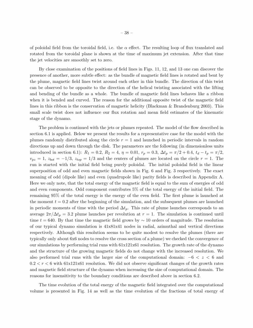
– 38 –

of poloidal field from the toroidal field, i.e. the α effect. The resulting loop of flux translated and

rotated from the toroidal plane is shown at the time of maximum jet extension. After that time

the jet velocities are smoothly set to zero.

By close examination of the positions of field lines in Figs. 11, 12, and 13 one can discover the

presence of another, more subtle effect: as the bundle of magnetic field lines is rotated and bent by

the plume, magnetic field lines twist around each other in this bundle. The direction of this twist

can be observed to be opposite to the direction of the helical twisting associated with the lifting

and bending of the bundle as a whole. The bundle of magnetic field lines behaves like a ribbon

when it is bended and curved. The reason for the additional opposite twist of the magnetic field

lines in this ribbon is the conservation of magnetic helicity (Blackman & Brandenburg 2003). This

small scale twist does not influence our flux rotation and mean field estimates of the kinematic

stage of the dynamo.

The problem is continued with the jets or plumes repeated. The model of the flow described in

section 6.1 is applied. Below we present the results for a representative case for the model with the

plumes randomly distributed along the circle r = 1 and launched in periodic intervals in random

directions up and down through the disk. The parameters are the following (in dimensionless units

introduced in section 6.1): R1 = 0.2, R2 = 4, η = 0.01, rp = 0.3, ∆tp = π/2 + 0.4, td − tp = π/2,

vpz = 1, zbot = −1/3, ztop = 1/3 and the centers of plumes are located on the circle r = 1. The

run is started with the initial field being purely poloidal. The initial poloidal field is the linear

superposition of odd and even magnetic fields shown in Fig. 6 and Fig. 3 respectively. The exact

meaning of odd (dipole like) and even (quadrupole like) parity fields is described in Appendix A.

Here we only note, that the total energy of the magnetic field is equal to the sum of energies of odd

and even components. Odd component contributes 5% of the total energy of the initial field. The

remaining 95% of the total energy is the energy of the even field. The first plume is launched at

the moment t = 0.2 after the beginning of the simulation, and the subsequent plumes are launched

in periodic moments of time with the period ∆tp. This rate of plume launches corresponds to an

average 2π/∆tp = 3.2 plume launches per revolution at r = 1. The simulation is continued until

time t = 640. By that time the magnetic field grows by ∼ 10 orders of magnitude. The resolution

of our typical dynamo simulation is 41x81x41 nodes in radial, azimuthal and vertical directions

respectively. Although this resolution seems to be quite modest to resolve the plumes (there are

typically only about 6x6 nodes to resolve the cross section of a plume) we checked the convergence of

our simulations by performing trial runs with 61x121x61 resolution. The growth rate of the dynamo

and the structure of the growing magnetic fields do not change with the increased resolution. We

also performed trial runs with the larger size of the computational domain: −6 < z < 6 and

0.2 < r < 6 with 61x121x61 resolution. We did not observe significant changes of the growth rates

and magnetic field structure of the dynamo when increasing the size of computational domain. The

reasons for insensitivity to the boundary conditions are described above in section 6.2.

The time evolution of the total energy of the magnetic field integrated over the computational

volume is presented in Fig. 14 as well as the time evolution of the fractions of total energy of

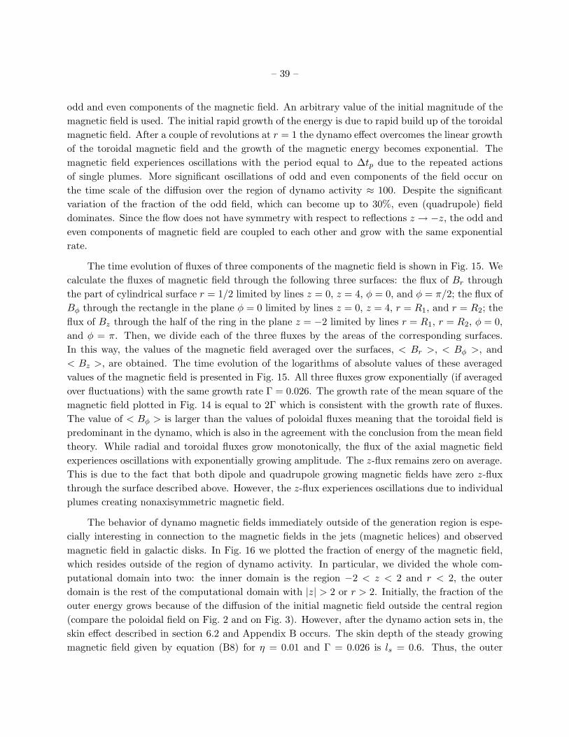
– 39 –

odd and even components of the magnetic field. An arbitrary value of the initial magnitude of the

magnetic field is used. The initial rapid growth of the energy is due to rapid build up of the toroidal

magnetic field. After a couple of revolutions at r = 1 the dynamo effect overcomes the linear growth

of the toroidal magnetic field and the growth of the magnetic energy becomes exponential. The

magnetic field experiences oscillations with the period equal to ∆tp due to the repeated actions

of single plumes. More significant oscillations of odd and even components of the field occur on

the time scale of the diffusion over the region of dynamo activity ≈ 100. Despite the significant

variation of the fraction of the odd field, which can become up to 30%, even (quadrupole) field

dominates. Since the flow does not have symmetry with respect to reflections z → −z, the odd and

even components of magnetic field are coupled to each other and grow with the same exponential

rate.

The time evolution of fluxes of three components of the magnetic field is shown in Fig. 15. We

calculate the fluxes of magnetic field through the following three surfaces: the flux of Br through

the part of cylindrical surface r = 1/2 limited by lines z = 0, z = 4, φ = 0, and φ = π/2; the flux of

Bφ through the rectangle in the plane φ = 0 limited by lines z = 0, z = 4, r = R1, and r = R2; the

flux of Bz through the half of the ring in the plane z = −2 limited by lines r = R1, r = R2, φ = 0,

and φ = π. Then, we divide each of the three fluxes by the areas of the corresponding surfaces.

In this way, the values of the magnetic field averaged over the surfaces, < Br >, < Bφ >, and

< Bz >, are obtained. The time evolution of the logarithms of absolute values of these averaged

values of the magnetic field is presented in Fig. 15. All three fluxes grow exponentially (if averaged

over fluctuations) with the same growth rate Γ = 0.026. The growth rate of the mean square of the

magnetic field plotted in Fig. 14 is equal to 2Γ which is consistent with the growth rate of fluxes.

The value of < Bφ > is larger than the values of poloidal fluxes meaning that the toroidal field is

predominant in the dynamo, which is also in the agreement with the conclusion from the mean field

theory. While radial and toroidal fluxes grow monotonically, the flux of the axial magnetic field

experiences oscillations with exponentially growing amplitude. The z-flux remains zero on average.

This is due to the fact that both dipole and quadrupole growing magnetic fields have zero z-flux

through the surface described above. However, the z-flux experiences oscillations due to individual

plumes creating nonaxisymmetric magnetic field.

The behavior of dynamo magnetic fields immediately outside of the generation region is espe-

cially interesting in connection to the magnetic fields in the jets (magnetic helices) and observed

magnetic field in galactic disks. In Fig. 16 we plotted the fraction of energy of the magnetic field,

which resides outside of the region of dynamo activity. In particular, we divided the whole com-

putational domain into two: the inner domain is the region −2 < z < 2 and r < 2, the outer

domain is the rest of the computational domain with |z| > 2 or r > 2. Initially, the fraction of the

outer energy grows because of the diffusion of the initial magnetic field outside the central region

(compare the poloidal field on Fig. 2 and on Fig. 3). However, after the dynamo action sets in, the

skin effect described in section 6.2 and Appendix B occurs. The skin depth of the steady growing

magnetic field given by equation (B8) for η = 0.01 and Γ = 0.026 is ls = 0.6. Thus, the outer

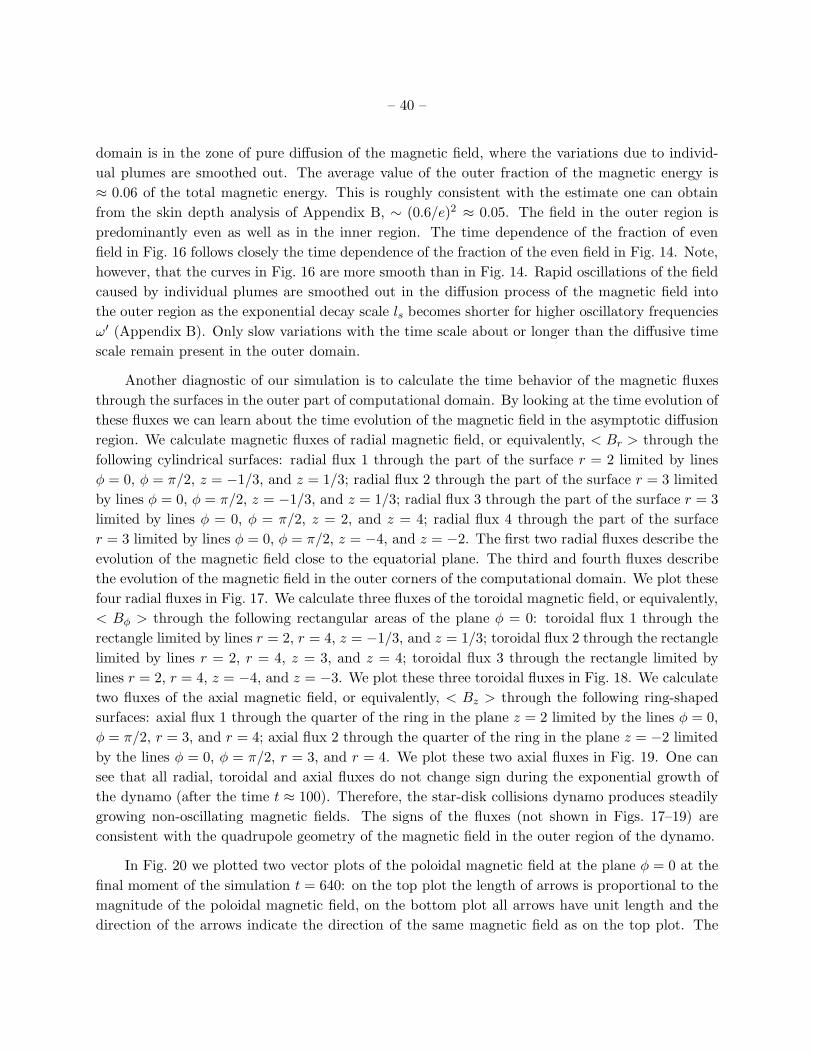
– 40 –

domain is in the zone of pure diffusion of the magnetic field, where the variations due to individ-

ual plumes are smoothed out. The average value of the outer fraction of the magnetic energy is

≈ 0.06 of the total magnetic energy. This is roughly consistent with the estimate one can obtain

from the skin depth analysis of Appendix B, ∼ (0.6/e)2 ≈ 0.05. The field in the outer region is

predominantly even as well as in the inner region. The time dependence of the fraction of even

field in Fig. 16 follows closely the time dependence of the fraction of the even field in Fig. 14. Note,

however, that the curves in Fig. 16 are more smooth than in Fig. 14. Rapid oscillations of the field

caused by individual plumes are smoothed out in the diffusion process of the magnetic field into

the outer region as the exponential decay scale ls becomes shorter for higher oscillatory frequencies

ω′ (Appendix B). Only slow variations with the time scale about or longer than the diffusive time

scale remain present in the outer domain.

Another diagnostic of our simulation is to calculate the time behavior of the magnetic fluxes

through the surfaces in the outer part of computational domain. By looking at the time evolution of

these fluxes we can learn about the time evolution of the magnetic field in the asymptotic diffusion

region. We calculate magnetic fluxes of radial magnetic field, or equivalently, < Br > through the

following cylindrical surfaces: radial flux 1 through the part of the surface r = 2 limited by lines

φ = 0, φ = π/2, z = −1/3, and z = 1/3; radial flux 2 through the part of the surface r = 3 limited

by lines φ = 0, φ = π/2, z = −1/3, and z = 1/3; radial flux 3 through the part of the surface r = 3

limited by lines φ = 0, φ = π/2, z = 2, and z = 4; radial flux 4 through the part of the surface

r = 3 limited by lines φ = 0, φ = π/2, z = −4, and z = −2. The first two radial fluxes describe the

evolution of the magnetic field close to the equatorial plane. The third and fourth fluxes describe

the evolution of the magnetic field in the outer corners of the computational domain. We plot these

four radial fluxes in Fig. 17. We calculate three fluxes of the toroidal magnetic field, or equivalently,

< Bφ > through the following rectangular areas of the plane φ = 0: toroidal flux 1 through the

rectangle limited by lines r = 2, r = 4, z = −1/3, and z = 1/3; toroidal flux 2 through the rectangle

limited by lines r = 2, r = 4, z = 3, and z = 4; toroidal flux 3 through the rectangle limited by

lines r = 2, r = 4, z = −4, and z = −3. We plot these three toroidal fluxes in Fig. 18. We calculate

two fluxes of the axial magnetic field, or equivalently, < Bz > through the following ring-shaped

surfaces: axial flux 1 through the quarter of the ring in the plane z = 2 limited by the lines φ = 0,

φ = π/2, r = 3, and r = 4; axial flux 2 through the quarter of the ring in the plane z = −2 limited

by the lines φ = 0, φ = π/2, r = 3, and r = 4. We plot these two axial fluxes in Fig. 19. One can

see that all radial, toroidal and axial fluxes do not change sign during the exponential growth of

the dynamo (after the time t ≈ 100). Therefore, the star-disk collisions dynamo produces steadily

growing non-oscillating magnetic fields. The signs of the fluxes (not shown in Figs. 17–19) are

consistent with the quadrupole geometry of the magnetic field in the outer region of the dynamo.

In Fig. 20 we plotted two vector plots of the poloidal magnetic field at the plane φ = 0 at the

final moment of the simulation t = 640: on the top plot the length of arrows is proportional to the

magnitude of the poloidal magnetic field, on the bottom plot all arrows have unit length and the

direction of the arrows indicate the direction of the same magnetic field as on the top plot. The

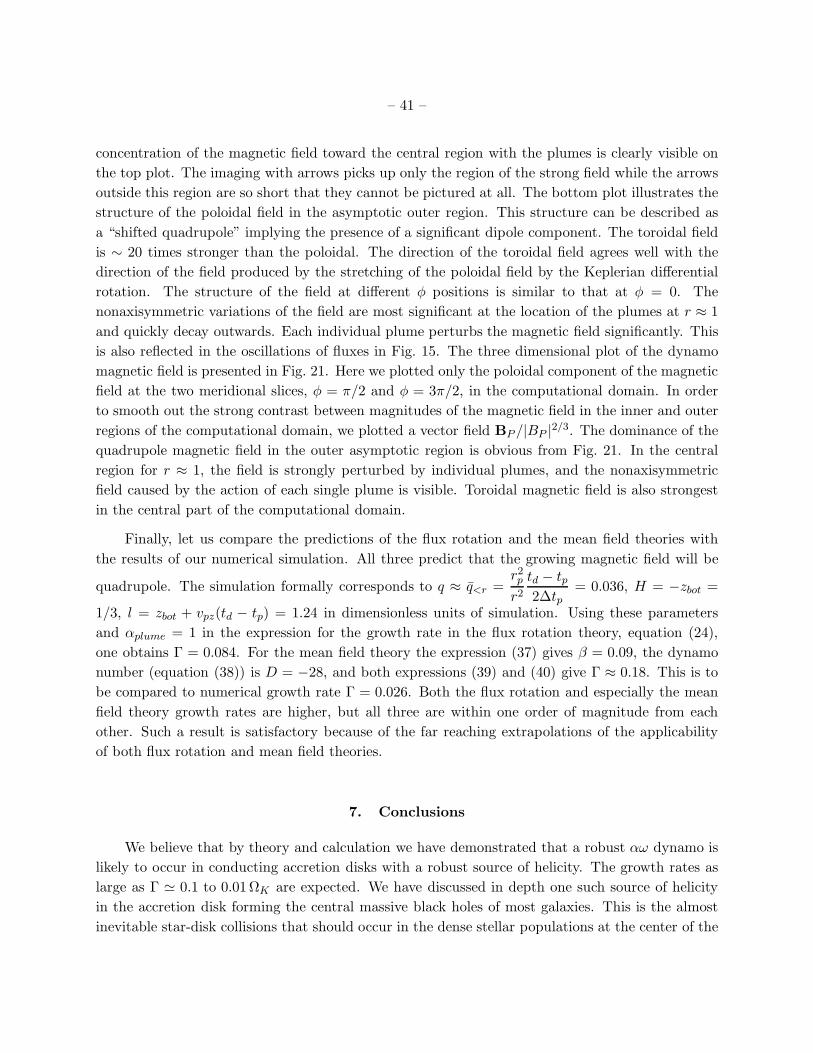
– 41 –

concentration of the magnetic field toward the central region with the plumes is clearly visible on

the top plot. The imaging with arrows picks up only the region of the strong field while the arrows

outside this region are so short that they cannot be pictured at all. The bottom plot illustrates the

structure of the poloidal field in the asymptotic outer region. This structure can be described as

a “shifted quadrupole” implying the presence of a significant dipole component. The toroidal field

is ∼ 20 times stronger than the poloidal. The direction of the toroidal field agrees well with the

direction of the field produced by the stretching of the poloidal field by the Keplerian differential

rotation. The structure of the field at different φ positions is similar to that at φ = 0. The

nonaxisymmetric variations of the field are most significant at the location of the plumes at r ≈ 1

and quickly decay outwards. Each individual plume perturbs the magnetic field significantly. This

is also reflected in the oscillations of fluxes in Fig. 15. The three dimensional plot of the dynamo

magnetic field is presented in Fig. 21. Here we plotted only the poloidal component of the magnetic

field at the two meridional slices, φ = π/2 and φ = 3π/2, in the computational domain. In order

to smooth out the strong contrast between magnitudes of the magnetic field in the inner and outer

regions of the computational domain, we plotted a vector field BP /|BP |2/3. The dominance of the

quadrupole magnetic field in the outer asymptotic region is obvious from Fig. 21. In the central

region for r ≈ 1, the field is strongly perturbed by individual plumes, and the nonaxisymmetric

field caused by the action of each single plume is visible. Toroidal magnetic field is also strongest

in the central part of the computational domain.

Finally, let us compare the predictions of the flux rotation and the mean field theories with

the results of our numerical simulation. All three predict that the growing magnetic field will be

quadrupole. The simulation formally corresponds to q ≈ q<r =r2p

r2

td − tp2∆tp

= 0.036, H = −zbot =

1/3, l = zbot + vpz(td − tp) = 1.24 in dimensionless units of simulation. Using these parameters

and αplume = 1 in the expression for the growth rate in the flux rotation theory, equation (24),

one obtains Γ = 0.084. For the mean field theory the expression (37) gives β = 0.09, the dynamo

number (equation (38)) is D = −28, and both expressions (39) and (40) give Γ ≈ 0.18. This is to

be compared to numerical growth rate Γ = 0.026. Both the flux rotation and especially the mean

field theory growth rates are higher, but all three are within one order of magnitude from each

other. Such a result is satisfactory because of the far reaching extrapolations of the applicability

of both flux rotation and mean field theories.

7. Conclusions

We believe that by theory and calculation we have demonstrated that a robust αω dynamo is

likely to occur in conducting accretion disks with a robust source of helicity. The growth rates as

large as Γ ≃ 0.1 to 0.01ΩK are expected. We have discussed in depth one such source of helicity

in the accretion disk forming the central massive black holes of most galaxies. This is the almost

inevitable star-disk collisions that should occur in the dense stellar populations at the center of the

– 42 –

galaxy. We estimate that this source of helicity is far larger than necessary for the dynamo fields to

reach saturation in less than the formation time of the black hole. Star-disk collisions should also

be the most robust source of helicity because the resulting plumes are driven several scale heights

above the surface of the disk as compared to turbulence were the vertical motions are limited to

a fraction of a scale height. The advantage of the αω dynamo is that because it produces a large

scale coherent field outside the disk, the poloidal field, the differential winding of this poloidal field

leads to a large scale force-free helix that transports the magnetic energy away from the disk and

from the dynamo. The back reaction of this force-free field (force-free except at the disk surface

boundary) only acts as a torque on the Keplerian flow and thus the field energy of the force-free

helix can grow at the expense of the free energy of formation of the black hole. The back reaction of

this force-free field, being much smaller than the toroidal field, does not affect the plume formation

by star-disk collisions. Only the much larger toroidal field affects the plumes and this in turn must

be less than the pressure inside the disk. Thus the star disk collisions produce a robust dynamo

where the back reaction does not quench the dynamo action at low values of field. The resulting

exponential gain of this dynamo is an instability converting kinetic to magnetic energy. Since the

gain is large, the dynamo fields should rapidly grow to saturation or the back reaction limit. This

limit we conjecture is the torque corresponding to the accretion flow of angular momentum away

from the black hole. Hence, the dynamo should convert a large fraction of the free energy of the

black hole formation to magnetic energy.

VP is pleased to thank Richard Lovelace and Eric Blackman for helpful discussions and Ben-

jamin Bromley for support with computer simulations. Eric Blackman is thanked again for his

support during the late stages of this work. The facilities and interactions of Aspen Center for

Physics are gratefully acknowledged, and particular support has been given by Hui Li through the

support of the Director Funded Research, ”Active Galaxies”. We are particularly pleased to ac-

knowledge the careful reading of the text by the anonymous referee and furthermore the significant

improvement of readability and putting our work in more perspective due to the referee’s efforts.

This work has been supported by the U.S. Department of Energy through the LDRD program at

Los Alamos National Laboratory. VP also acknowledges partial support by DOE grant DE-FG02-

00ER54600 and by the Center for Magnetic Self-Organization in Laboratory and Astrophysical

Plasmas at University of Wisconsin-Madison . The Cray supercomputer used in this research was

provided through funding from the NASA Offices of Space Sciences, Aeronautics, and Mission to

Planet Earth.

A. On the Parity of Magnetic Fields

Any arbitrary vector field C = C(r, φ, z) can be decomposed into the sum of parts even and

odd with respect to the reflection z → −z, C = Ce + Co. The following symmetry rules are valid

– 43 –

for an even field:

Cer (−z) = Ce

r (z), Ceφ(−z) = Ce

φ(z), Cez (−z) = −Ce

z (z), (A1)

and for an odd field:

Cor (−z) = −Co

r (z), Coφ(−z) = −Co

φ(z), Coz (−z) = Co

z (z). (A2)

Often even fields are called quadrupole type fields and odd fields are called dipole type fields.

The last terminology reflects on the largest scale modes possible within each symmetry class and

allows one to visualize fields of each symmetry type easily. The even and odd decomposition of an

arbitrary field C can be performed as follows:

Cer (r, φ, z) =

1

2(C(r, φ, z) + C(r, φ,−z)), (A3a)

Ceφ(r, φ, z) =

1

2(C(r, φ, z) + C(r, φ,−z)), (A3b)

Cez (r, φ, z) =

1

2(C(r, φ, z) − C(r, φ,−z)), (A3c)

Cor (r, φ, z) =

1

2(C(r, φ, z) − C(r, φ,−z)), (A3d)

Coφ(r, φ, z) =

1

2(C(r, φ, z) − C(r, φ,−z)), (A3e)

Coz (r, φ, z) =

1

2(C(r, φ, z) + C(r, φ,−z)). (A3f)

One can check that for any volume V symmetric with respect to the plane z = 0∫

VC2 dV =

∫

V(Ce)2 dV +

∫

V(Co)2 dV . (A4)

This implies that if C = B is a magnetic field, then the energy of the magnetic field is equal

to the sum of the energies of its even and odd components. The even and odd components of

solutions of equations (34) and (35) decouples if the mean velocity field is even, vPr(−z) = vPr(z),

vPz(−z) = −vPz(z), Ω(−z) = Ω(z), the coefficient α is antisymmetric with respect to reflection

z → −z, and the coefficient β is symmetric with respect to reflection z → −z. Thus, even

(quadrupole) and odd (dipole) modes will have different growth rates. The axisymmetric magnetic

field is even if A(−z) = −A(z), Bφ(z) = Bφ(−z) and is odd if A(−z) = A(z), Bφ(−z) = −Bφ(z).

B. Skin Effect for the Magnetic Dynamo

Let us consider equation (72) written in spherical coordinates , θ, and φ such that θ = 0

and θ = π corresponds to the symmetry axis of the system. In the case of time-dependent flow

described in section 6.1 there are no eigenmodes with a fixed frequency. Instead, the magnetic

field can be represented as an integral over frequencies in the Fourier transformation. However,

– 44 –

in the case of a growing (and possibly oscillating) magnetic field, there is a characteristic growth

rate Γ of the dynamo averaged over plume pulses. In addition, the magnetic field will possess

oscillating Fourier components associated with the period of the emergence of plumes and, possibly,

some intrinsic oscillatory behavior of the dynamo. We consider the behavior of one such Fourier

component assuming the dependence A ∝ exp(−iωt), where the complex ω is the sum of the real

and imaginary parts as ω = ω′ + iΓ. The Γ is the average growth rate of the dynamo, while ω′ can

take on a whole range of values, including the frequency of plumes, the Keplerian period, all its

harmonics, etc. We impose the boundary condition for A on some sphere of radius in such that

in > 1 but still in is of the order of 1. We assume that the value of A at = in is dictated by

the dynamo process inside in. Then, for one Fourier component equation (72) becomes

−iωA

η=

1

2

∂

∂

(

2 ∂A

∂

)

+1

2LA, (B1)

where

L =1

sin θ

∂

∂θ

(

sin θ∂

∂θ

)

− 1

sin2 θ

is the angular operator acting on A. In spherical geometry, equation (B1) has separable variables

and θ. Thus, we look for solutions in the form A = Rl()Ql(θ) exp(−iωt).

The operator L commonly occurs in problems with axisymmetric flows, when solving the

equation for the stream function. Since the magnetic field should be finite on the axis θ = 0, the

quantity1

sin θ

∂

∂θ(sin θA)

must be finite at θ = 0 and at θ = π, because BP = ∇× (Aeφ). The eigenvalues and eigenfunctions

LQl = λlQl satisfying these boundary conditions are

λl = −l(l + 1), Ql = sin θP ′

l (cos θ), (B2)

where prime denotes the differentiation of the Legendre polynomial Pl(x) with respect to x and

l = 1, 2, 3, . . . Besides these eigenvalues, λ = 0 is also an eigenvalue with the eigenfunction Q0 =

(1 − cos θ)/ sin θ. The first three eigenfunctions given by formula (B2) are

Q1 = sin θ, Q2 = sin θ cos θ, Q3 = sin θ

(

cos2 θ − 1

5

)

. (B3)

The angular dependence Ql(θ) determines the symmetry of the solutions. The mode proportional

to Q0 describes the radially directed magnetic field with nonzero total flux through the sphere from

θ = 0 to θ = π. All terms with l ≥ 1 corresponds to the magnetic field with vanishing total flux

through the sphere from θ = 0 to θ = π. The Q0 term cannot be excited by the dynamo operating

inside in because of ∇·B = 0 condition. This is also clear from the fact that Q0 → ∞ when θ → π,

which means that the vector potential cannot be well defined for a magnetic field with ∇ · B 6= 0.

The terms with l ≥ 1 represent multipole expansion of the magnetic field in the far zone of the

generation region. R1()Q1(θ) is a dipole term, R2()Q2(θ) is a quadrupole term, and so on.

– 45 –

For the radial part of the solution we obtain the equation

d2Rl

d2+

2

dRl

d− l(l + 1)

2Rl −

Γ − iω′

ηRl = 0. (B4)

We introduce a new variable z = /χ where

χ2 =η(Γ + iω′)

Γ2 + ω′2. (B5)

Then, equation (B4) reduces to the Bessel equation of imaginary argument. Solutions of this

equation which vanishes at → ∞ are given in terms of modified Bessel function Kν(z) as

Rl =

√

π

2zKl+1/2(z).

The Bessel functions of half-integer order can be expressed through elementary functions (e.g.,

Abramowitz & Stegun (1972)). Thus, we obtain for the dipole and quadrupole terms

R1(z) =π

2ze−z

(

1 +1

z

)

, R2(z) =π

2ze−z

(

1 +3

z+

3

z2

)

.

Finally, collecting all the terms together and retaining only the leading dipole and quadrupole

terms, we obtain the following solution for A

A = a1 sin θπχ

2e−/χ

(

1 +χ

)

e−iωt +

a2 sin θ cos θπχ

2e−/χ

(

1 +3χ

+

3χ2

2

)

e−iωt, (B6)

where the coefficients a1 and a2 should be determined by the condition of the continuity of harmonics

of A at the surface = in. The values of a1 and a2 are determined by the dynamo action inside

the radius in. We see that both dipole and quadrupole components (and all higher multipole

components) decay as ∝ e−/χ. Using the expression (B5) for χ one obtains

e−/χ = exp

(

− √2η

√

√

Γ2 + ω′2 + Γ + i√2η

√

√

Γ2 + ω′2 − Γ

)

, (B7)

where we assumed Γ > 0 and ω′ > 0. The thickness of the skin layer is determined by the real part

of the expression under the exponent in equation (B7). The larger the growth rate Γ, the faster the

magnetic field decays with the radius. Also, oscillating modes with ω′ > 0 decay faster with the

radius than the steady modes with ω′ = 0. Thus, far from the dynamo source one should expect

the magnetic field to be growing in time, steadily, without oscillations.

The characteristic length of the exponential decay of the field, ls, is found from equation (B7)

as

ls =

√

2η√Γ2 + ω′2 + Γ

. (B8)

For a steady magnetic field ls =√

η/Γ. When is approaching the radius of the outer boundary

R2, the solution (B6) starts to “feel” the boundary condition as an ideally conducting boundary

and the numerical results at ≥ R2 are not approximated by formula (B6).

– 46 –

REFERENCES

Abramowitz, M., & Stegun, I. A. 1972, Handbook of Mathematical Functions. (New York: Dover)

Bayliss, R.A., Nornberg, M.D., Terry, P.W., & Forest, C.B. 2006, Phys. Rev. E, submitted

(arXiv:physics/0602126)

Beckley, H.F., Colgate, S.A., Romero, V.D., & Ferrel, R. 2003, ApJ, 599, 702

Biskamp, D. 1993, Nonlinear Magnetohydrodynamics. (Cambridge: Cambridge Univ. Press)

Blackman, E.G., & Brandenburg, A. 2003, ApJ, 584, L99

Blandford, R.D., & Payne, D.G. 1982, MNRAS, 199, 883

Boldyrev, S.A., & Cattaneo, F. 2004, Phys. Rev. Lett., 92, 144501

Boldyrev, S.A. 2006, Phys. Rev. Lett., 96, 115002

Bondi, H., & Hoyle, F. 1944, MNRAS, 104, 273

Bondi, H., Hoyle, F., & Lyttleton, R.A. 1947, MNRAS, 107, 184

Bondi, H. 1952, MNRAS, 112, 195

Bourgoin, M., Marie, L., Petrelis, F., Gasquet, C., Guigon, A., Luciani, J.-P., Moulin, M.,

Namer, F., et al. 2002, Phys. Fluids., 14, 3046

Bourgoin, M., Odier, P., Pinton, J.-F., & Ricard, Y. 2004, Phys. Fluids., 16, 2529

Busse, F.H. 1991, in Advances in Solar System Magnetohydrodynamics, eds. Priest E.R.,

Wood A.W. (Cambridge: Cambridge Univ. Press), p. 51

Chakrabarti, S.K., Rosner, R., & Vainshtein, S.I. 1994, Nature, 368, 434

Childress, S., Collet, P., Frish, U., Gilbert, A.D., Moffatt, H.K., & Zaslavsky, G.M. 1990, Geophys.

Astrophys. Fluid Dyn., 52, 263

Colgate, S.A., & Li, H. 1997, in Relativistic Jets in AGNs, ed. Ostrowski M. (Crakow: Poland),

p. 170

Colgate, S.A., & Li, H. 1999, Ap&SS, 264, 357

Colgate, S.A., Li, H., & Pariev, V.I. 2001, Physics of Plasmas, 8, 2425

Colgate, S.A., Cen, R., Li, H., Currier, N., & Warren, M.S. 2003, ApJ, 598, L7

Cowling, T.G. 1981, ARA&A, 19, 115

Dudley, M.L., & James, R.W. 1989 Proc. R. Soc. London A 425, 407

– 47 –

Ferriere, K., 1993a, ApJ, 404, 162

Ferriere, K., 1993b, ApJ, 409, 248

Ferriere, K., 1998, A&A, 335, 488

Ferriere, K., & Schmitt, D. 2000, A&A, 358, 125

Finn, J.M. 1992, in Electromechanical coupling of the solar atmosphere, Proceedings of the OSL

Workshop, (Capri, Italy), p. 79

Finn, J.M., Ott, E., Hanson, J.D., & Kan, I. 1991, Physics of Fluids, B3, 1250

Fletcher, C.A.J. 1992, Computational Techniques for Fluid Dynamics. (Heidelberg: Springer–

Verlag)

Frolov, V.P., & Novikov, I.D. 1998, Black Hole Physics: Basic Concepts and New Developments.

(Dordrecht: Kluwer)

Gailitis, A., & Freiberg, Ya. 1976, Magnetohydrodynamics, 12, 127

Gailitis, A., Lielausis, O., Dement’ev, S., et al. 2000, Phys. Rev. Lett., 84, 4365

Gailitis, A., Lielausis, O., Platacis, E., et al. 2001, Phys. Rev. Lett., 86, 3024

Goldreich, P., & Sridhar, S. 1995, ApJ, 438, 763

Hoyle, F. 1949, Some Recent Researches in Solar Physics. (Cambridge: University Press)

Iroshnikov, P.S. 1963, AZh, 40, 742

Khanna, R., & Camenzind, M., 1996a, A&A, 307, 665

Khanna, R., & Camenzind, M., 1996b, A&A, 313, 1028

Kraichnan, R.H. 1965, Phys. Fluids, 8, 1385

Krause, F., & Radler, K.H. 1980, Mean-Field Magnetohydrodynamics and Dynamo Theory. (Ox-

ford: Pergamon Press)

Kronberg, P.P., Dufton, Q.W., Li, H., & Colgate, S.A. 2001, ApJ, 560, 178

Kulsrud, R.M., 1999, ARA&A, 37, 37

Lau, Y.-T., & Finn, J.M. 1993, Physics of Fluids, B5, 365

Laval, J-P., Blaineau, P., Leprovost, N., Dubrulle, B., & Daviaud, F. 2006, Phys. Rev. Lett., 96,

204503

Li, H., Finn, J.M., Lovelace, R.V.E., & Colgate, S.A. 2000, ApJ, 533, 1023

– 48 –

Li, H., Lovelace, R.V.E., Finn, J.M., & Colgate, S.A. 2001a, ApJ, 561, 915

Li, H., Colgate, S.A., Wendroff, B., & Liska, R. 2001b, ApJ, 551, 874

Lovelace, R.V.E., Li, H., Colgate, S.A., & Nelson, A.F. 1999, ApJ, 513, 805

Marie, L., Burguete, J., Daviaud, F., & Leorat, J. 2003, European Physical Journal B, 33, 469

McCrea, W.H. 1953, MNRAS, 113, 162

Mestel, L. 1999, Stellar Magnetism. (Oxford: Clarendon)

Moffatt, H.K. 1978, Magnetic Field Generation in Electrically Conducting Fluids. (Cambridge:

Cambridge University Press)

Molchanov, S.A., Ruzmaikin, A.A., & Sokoloff, D.D. 1983, Magnetohydrodynamics, 19, 402

Nornberg, M.D., Spence, E.J., Kendrick R.D., & Forest C.B. 2006, Phys. Plasmas, 13, 055901

O’Connell, R., Kendrick, R.D., Nornberg, M.D., Spence, E.J., Bayliss, R.A., & Forest, C.B. 2005,

in Dynamo and Dynamics, a Mathematical Challenge, v.26 of NATO Science Series, eds.

Chossat, P., Ambruster, D., Oprea, I.

Ponty, Y., Mininni, P.D., Montgomery, D.C., Pinton, J.-F., Politano, H., & Pouquet, A. 2005,

Phys. Rev. Lett., 94, 164502

Pariev, V.I., & Colgate, S.A. 2006, ApJ, in press (paper I)

Parker, E.N. 1955, ApJ, 121, 29

Parker, E.N. 1979, Cosmical Magnetic Fields, their Origin and their Activity. (Oxford: Claredon)

Peffley, N.L., Cawthorne, A.B., & Lathrop, D.P. 2000, Phys. Rev. E, 61, 5287

Petrelis, F., Bourgoin, M., Marie, L., Burguete, J., Chiffaudel, A., Daviaud, F., Fauve, S., Odier, P.,

et al. 2003, Phys. Rev. Lett., 90, 174501.

Ponomarenko, Yu.B. 1973, J. Appl. Mech. Tech. Phys., 14, 775

Priest, E.R. 1982, Solar Magneto-hydrodynamics. (Boston: Kluwer, Inc.)

Reyes-Ruiz, M. & Stepinski, T.F., 1999, A&A, 342, 892

Roberts, P.H., & Soward, A.M. 1992, Ann. Rev. of Fluid Mechanics, 24, 459

Ruzmaikin, A.A., Sokoloff, D.D., & Shukurov, A.M. 1988, Magnetic fields in galaxies. (Moscow:

Nauka)

Sakharov, A.D. 1982, Selected Scientific Works. Divertissment 11. (New York: Marcel Dekker)

– 49 –

Shakura, N.I. 1972, AZh, 49, 921

Shakura, N.I., & Sunyaev, R.A. 1973, A&A, 24, 337

Sovinec, C.R., Finn, J.M., & del-Castillo-Negrete, D. 2001, Phys. Plasmas, 8, 475

Sisan, D.R., Mujica, N., Tillotson, W.A., Huang, Y.-M., Dorland, W., Hassam, A.B., Anton-

sen T.M., & Lathrop, D.P. 2004, Phys. Rev. Lett., 93, 114502

Spence, E.J., Nornberg, M.D., Jacobson, C.M., Kendrick R.D., & Forest, C.B. 2006, Phys. Rev.

Lett., 96, 055002

Steenbeck, M., Krause, F., & Radler, K.H. 1966, Z. Naturforsch., 21a, 369

Stepinski, T.F., & Levy, E.H. 1988, ApJ, 331, 416

Stieglitz, R., & Muller, U. 2001, Physics of Fluids, 13, 561

Stix, M. 1975, A&A, 42, 85

Sweet, D., Ott, E., Antonsen, T.M., Lathrop, D.P., & Finn, J.M. 2001, Physics of Plasmas, 8, 1944

Vainshtein, S.I., & Zeldovich, Ya.B. 1972, Soviet Physics Uspekhi, 15, 159

Zeldovich, Ya.B., Ruzmaikin, A.A., & Sokoloff, D.D. 1983, Magnetic Fields in Astrophysics. (New

York: Gordon and Breach Science Publishers)

This preprint was prepared with the AAS LATEX macros v5.0.

– 50 –

Fig. 1.— The α − Ω dynamo in a galactic black hole accretion disk. The radial component of the

poloidal quadrupole field within the disk (A) is sheared by the differential rotation within the disk,

developing a stronger toroidal component (B). As a star passes through the disk it heats by shock

and by radiation a fraction of the matter of the disk, which expands vertically and lifts a fraction of

the toroidal flux within an expanding plume (C). Due to the conservation of angular momentum,

the expanding plume and embedded flux rotate ∼ π/2 radians before the matter in the plume and

embedded flux falls back to the disk (D). Reconnection allows the new poloidal flux to merge with

and augment the original poloidal flux (D).

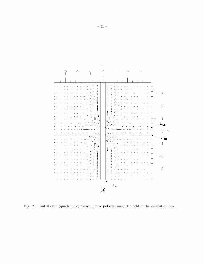
– 51 –

Fig. 2.— Initial even (quadrupole) axisymmetric poloidal magnetic field in the simulation box.

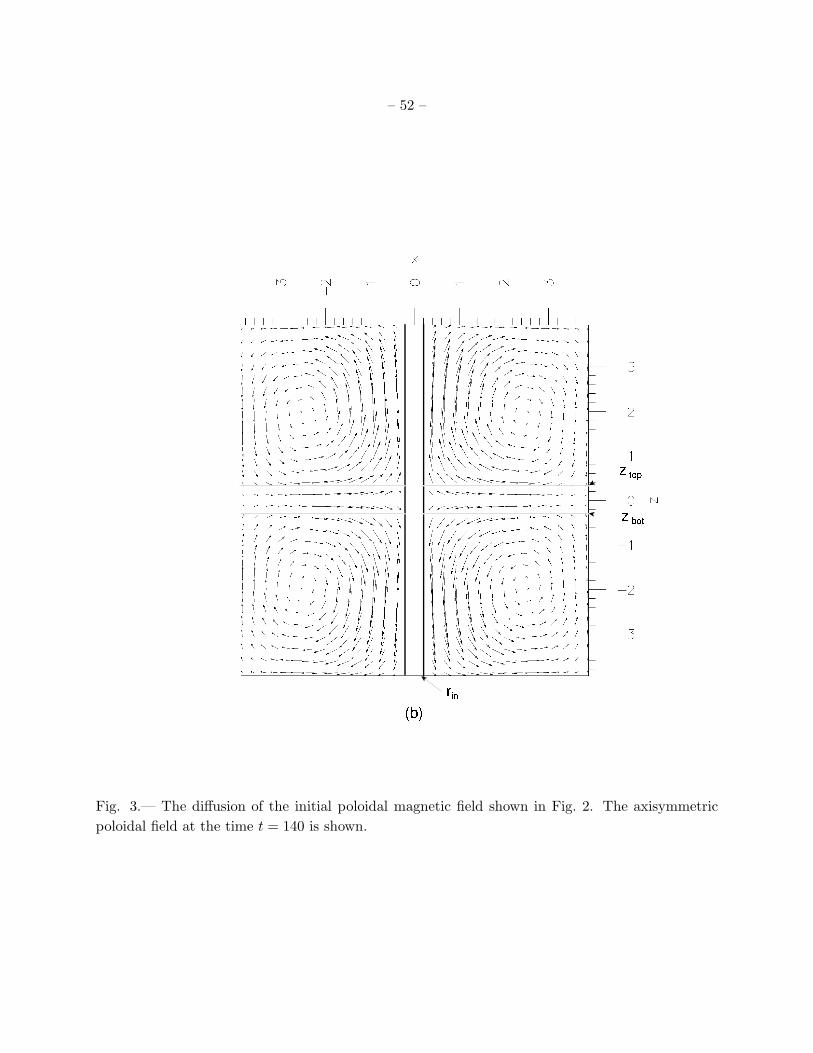
– 52 –

Fig. 3.— The diffusion of the initial poloidal magnetic field shown in Fig. 2. The axisymmetric

poloidal field at the time t = 140 is shown.

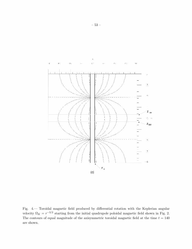
– 53 –

Fig. 4.— Toroidal magnetic field produced by differential rotation with the Keplerian angular

velocity ΩK = r−3/2 starting from the initial quadrupole poloidal magnetic field shown in Fig. 2.

The contours of equal magnitude of the axisymmetric toroidal magnetic field at the time t = 140

are shown.

– 54 –

Fig. 5.— Evolution of fluxes of three components of magnetic field for the simulation presented in

Figs. 2–4. Natural logarithms of the absolute value of fluxes are plotted vs. time. Flux of Br is

calculated through the part of the cylindrical surface r = 2 limited by lines φ = 0, φ = π/2, z = 0,

and z = 4. Flux of Bz is calculated through the surface z = 3 limited by lines r = R1, r = R2,

φ = 0, and φ = π. Flux of Bφ is calculated through the surface φ = 0 limited by lines r = R1,

r = R2, z = 0, and z = 4.

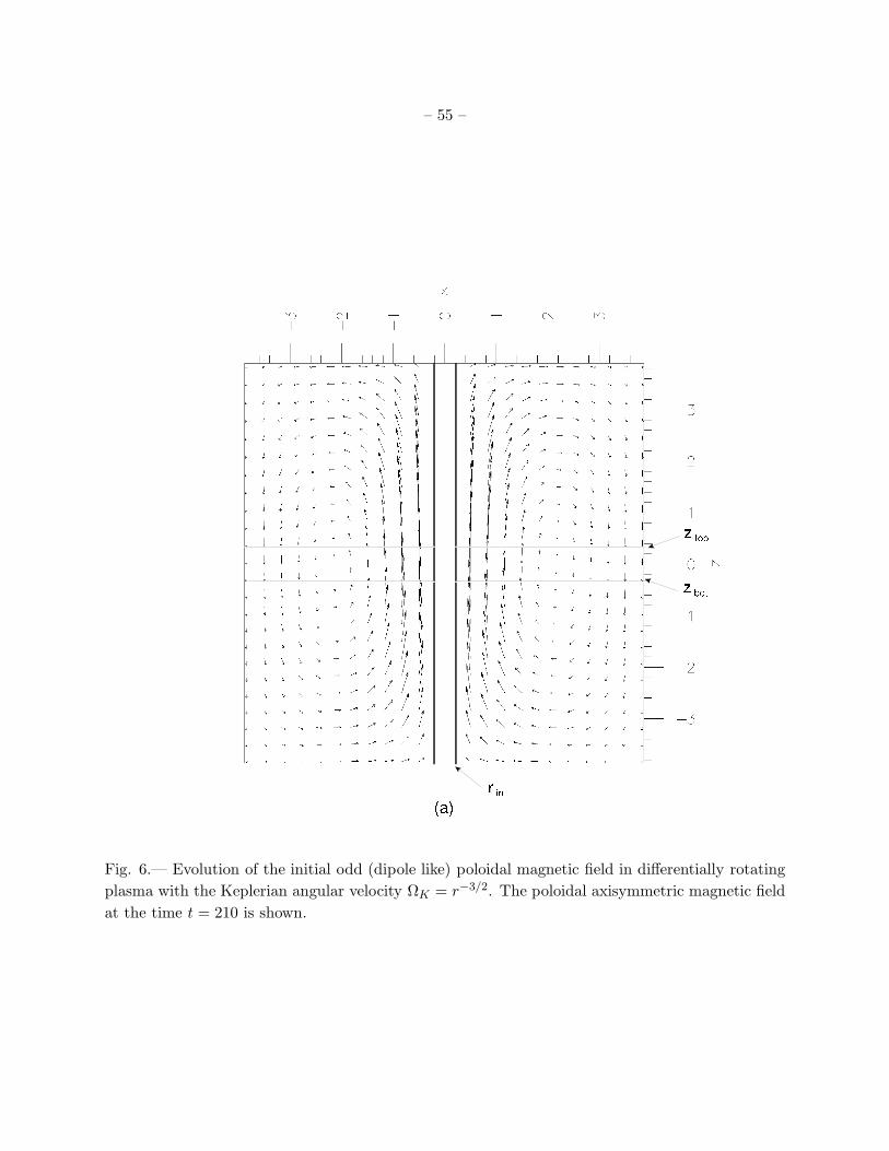
– 55 –

Fig. 6.— Evolution of the initial odd (dipole like) poloidal magnetic field in differentially rotating

plasma with the Keplerian angular velocity ΩK = r−3/2. The poloidal axisymmetric magnetic field

at the time t = 210 is shown.

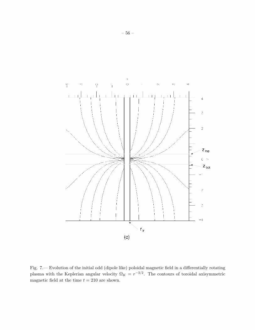
– 56 –

Fig. 7.— Evolution of the initial odd (dipole like) poloidal magnetic field in a differentially rotating

plasma with the Keplerian angular velocity ΩK = r−3/2. The contours of toroidal axisymmetric

magnetic field at the time t = 210 are shown.

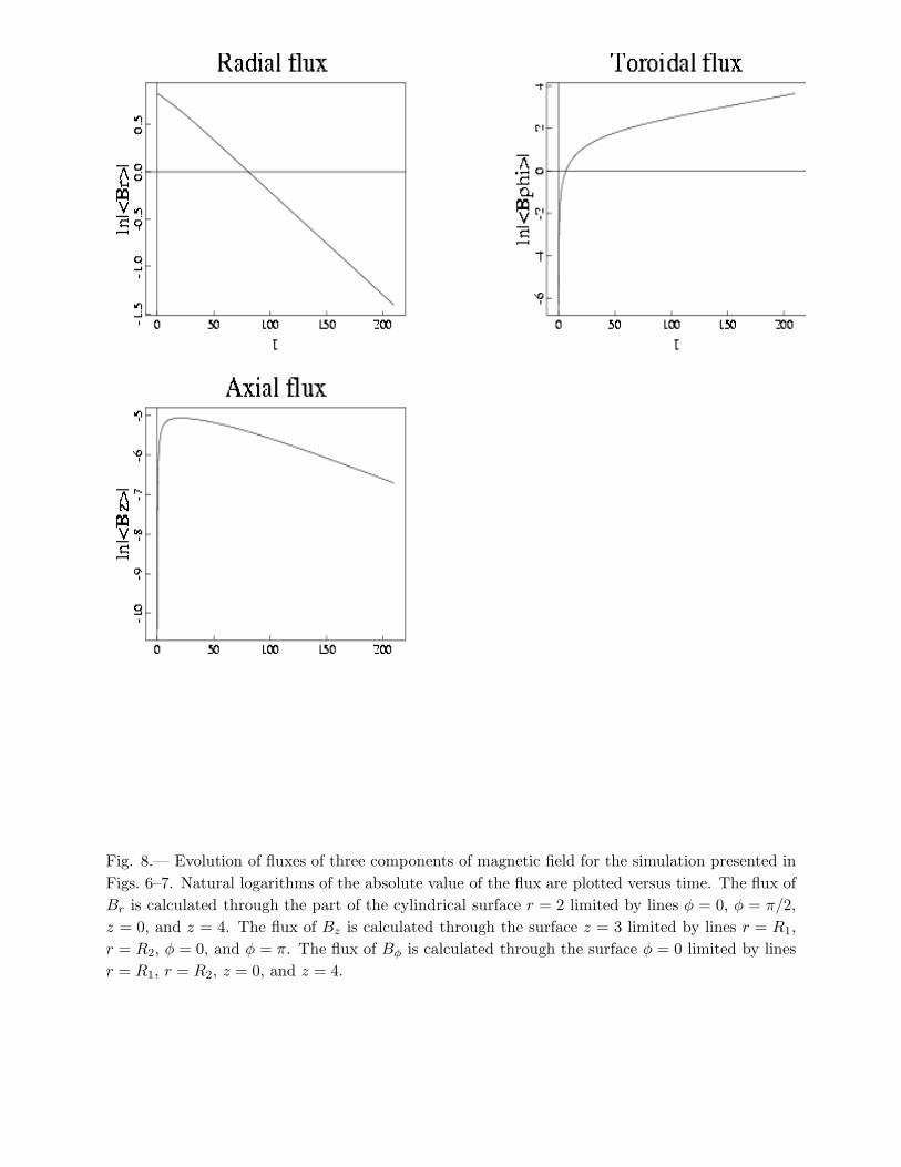
– 57 –

Fig. 8.— Evolution of fluxes of three components of magnetic field for the simulation presented in

Figs. 6–7. Natural logarithms of the absolute value of the flux are plotted versus time. The flux of

Br is calculated through the part of the cylindrical surface r = 2 limited by lines φ = 0, φ = π/2,

z = 0, and z = 4. The flux of Bz is calculated through the surface z = 3 limited by lines r = R1,

r = R2, φ = 0, and φ = π. The flux of Bφ is calculated through the surface φ = 0 limited by lines

r = R1, r = R2, z = 0, and z = 4.

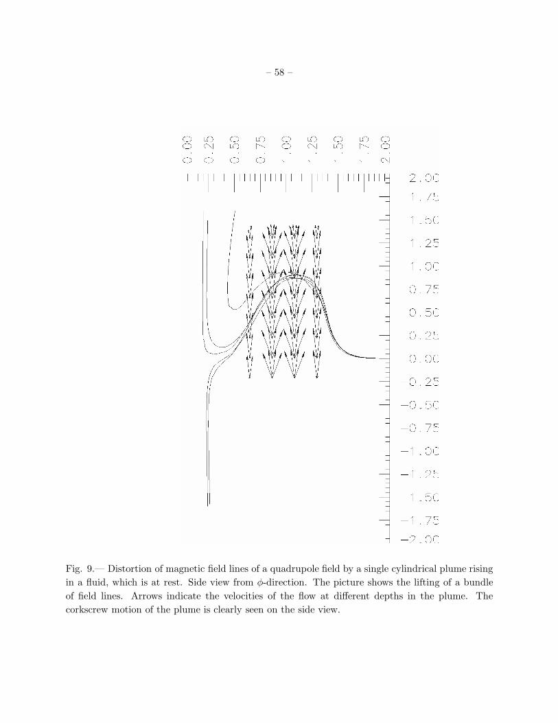
– 58 –

Fig. 9.— Distortion of magnetic field lines of a quadrupole field by a single cylindrical plume rising

in a fluid, which is at rest. Side view from φ-direction. The picture shows the lifting of a bundle

of field lines. Arrows indicate the velocities of the flow at different depths in the plume. The

corkscrew motion of the plume is clearly seen on the side view.

– 59 –

Fig. 10.— Same field configuration as in Fig. 9 viewed from the top z-direction. The picture shows

the twisting of the bundle of field lines. Arrows indicate velocities of the flow. The time is the same

as on Fig. 9.

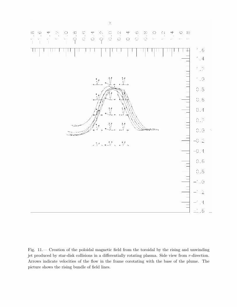
– 60 –

Fig. 11.— Creation of the poloidal magnetic field from the toroidal by the rising and unwinding

jet produced by star-disk collisions in a differentially rotating plasma. Side view from r-direction.

Arrows indicate velocities of the flow in the frame corotating with the base of the plume. The

picture shows the rising bundle of field lines.

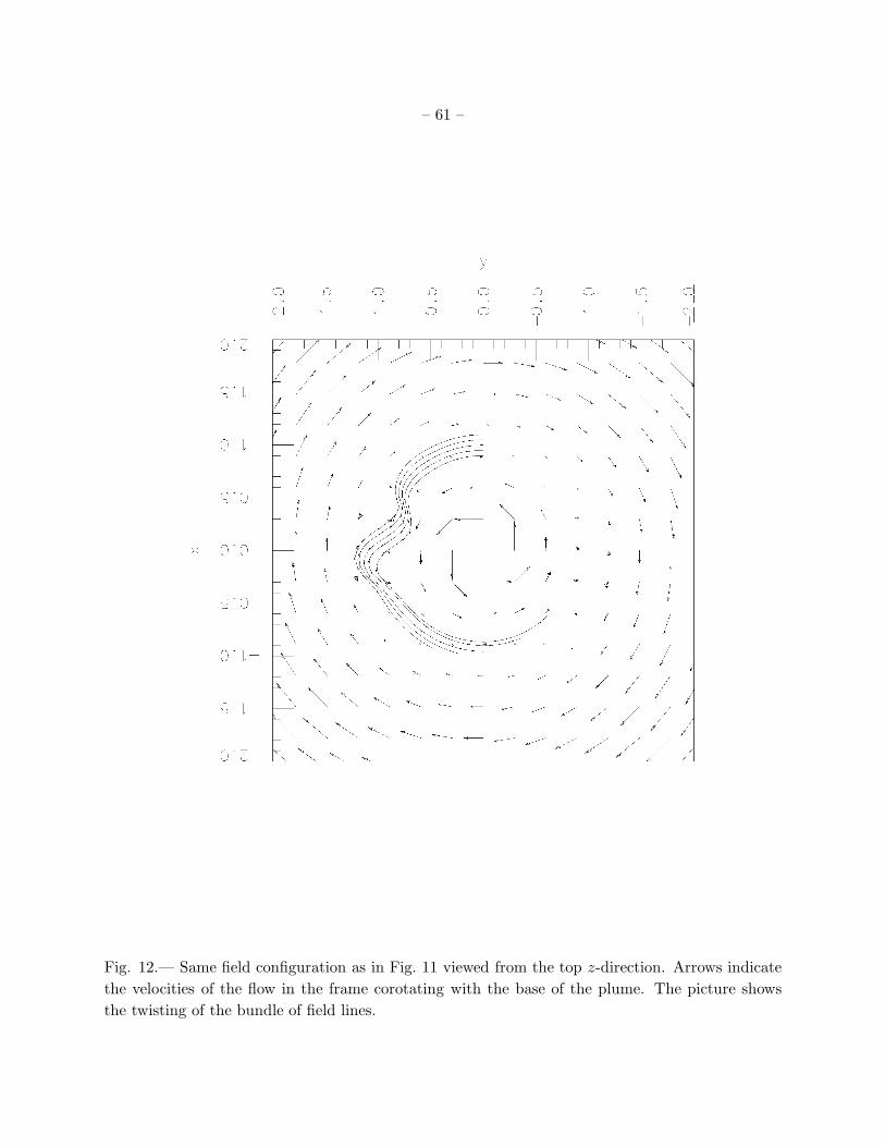
– 61 –

Fig. 12.— Same field configuration as in Fig. 11 viewed from the top z-direction. Arrows indicate

the velocities of the flow in the frame corotating with the base of the plume. The picture shows

the twisting of the bundle of field lines.

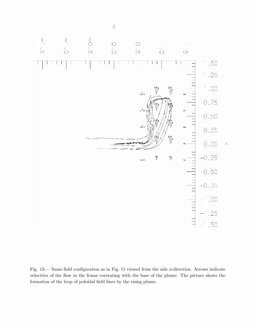
– 62 –

Fig. 13.— Same field configuration as in Fig. 11 viewed from the side φ-direction. Arrows indicate

velocities of the flow in the frame corotating with the base of the plume. The picture shows the

formation of the loop of poloidal field lines by the rising plume.

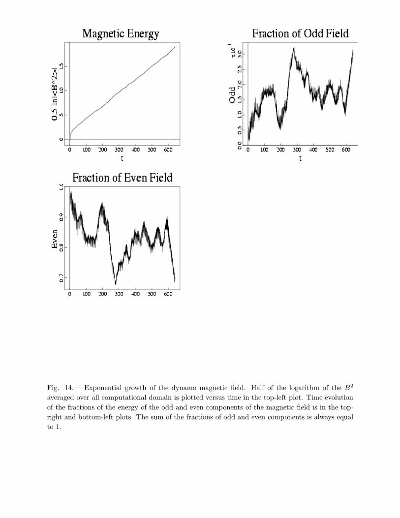
– 63 –

Fig. 14.— Exponential growth of the dynamo magnetic field. Half of the logarithm of the B2

averaged over all computational domain is plotted versus time in the top-left plot. Time evolution

of the fractions of the energy of the odd and even components of the magnetic field is in the top-

right and bottom-left plots. The sum of the fractions of odd and even components is always equal

to 1.

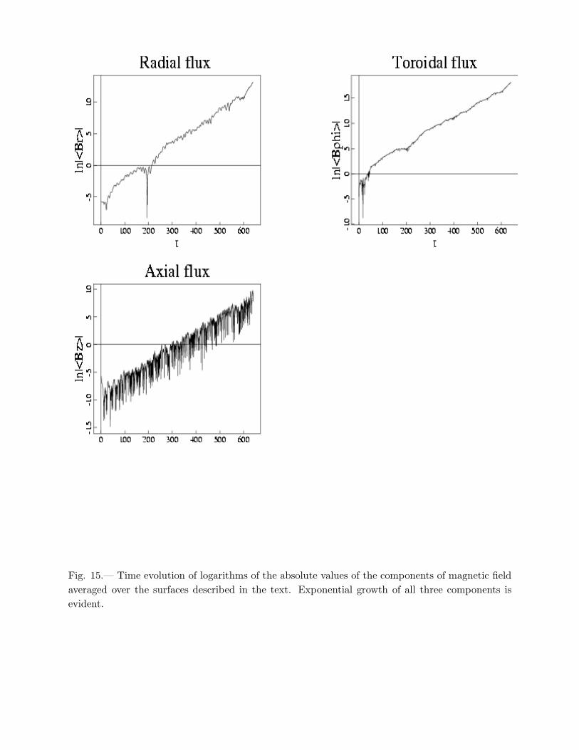
– 64 –

Fig. 15.— Time evolution of logarithms of the absolute values of the components of magnetic field

averaged over the surfaces described in the text. Exponential growth of all three components is

evident.

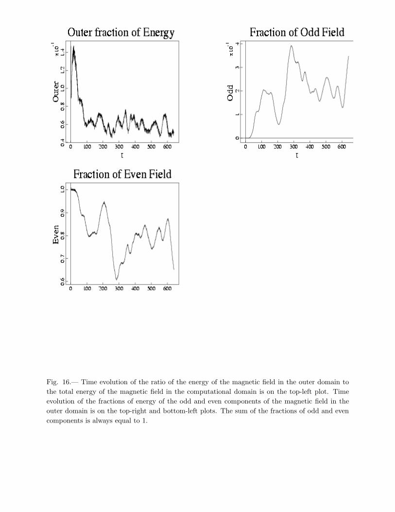
– 65 –

Fig. 16.— Time evolution of the ratio of the energy of the magnetic field in the outer domain to

the total energy of the magnetic field in the computational domain is on the top-left plot. Time

evolution of the fractions of energy of the odd and even components of the magnetic field in the

outer domain is on the top-right and bottom-left plots. The sum of the fractions of odd and even

components is always equal to 1.

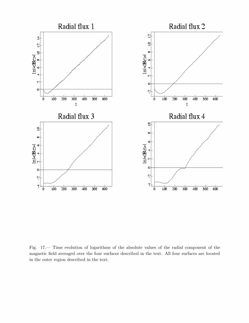
– 66 –

Fig. 17.— Time evolution of logarithms of the absolute values of the radial component of the

magnetic field averaged over the four surfaces described in the text. All four surfaces are located

in the outer region described in the text.

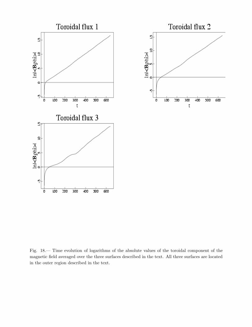
– 67 –

Fig. 18.— Time evolution of logarithms of the absolute values of the toroidal component of the

magnetic field averaged over the three surfaces described in the text. All three surfaces are located

in the outer region described in the text.

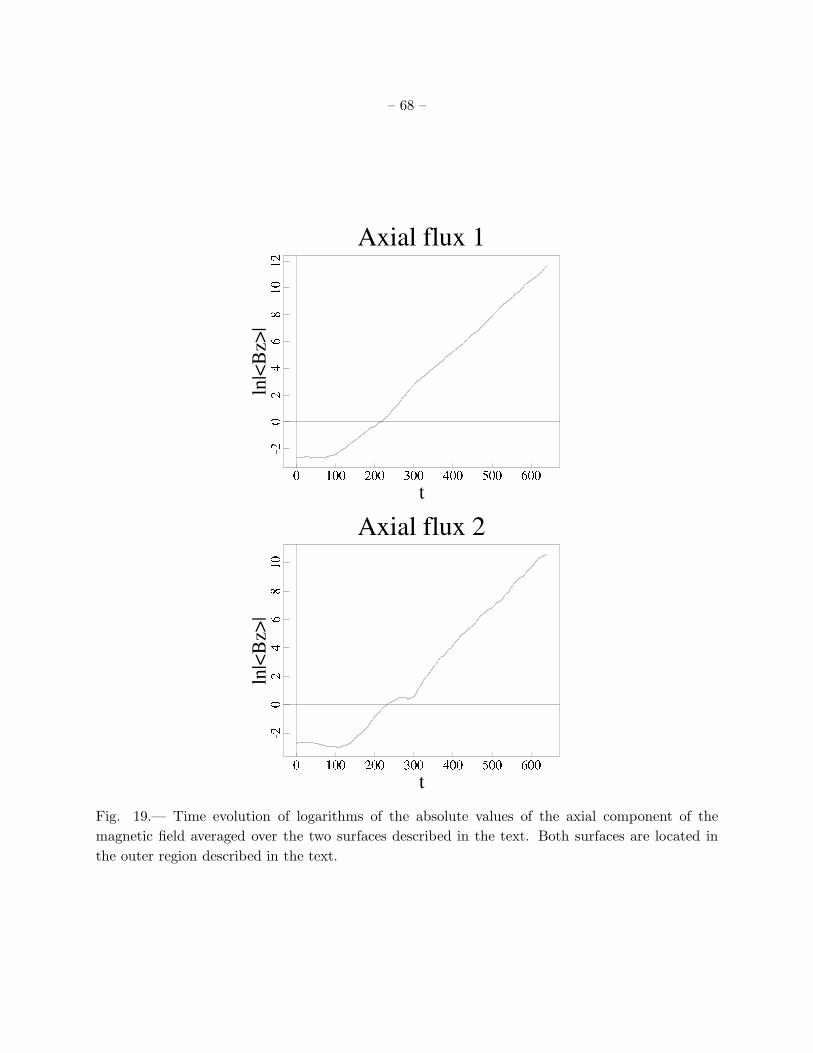
– 68 –

Fig. 19.— Time evolution of logarithms of the absolute values of the axial component of the

magnetic field averaged over the two surfaces described in the text. Both surfaces are located in

the outer region described in the text.

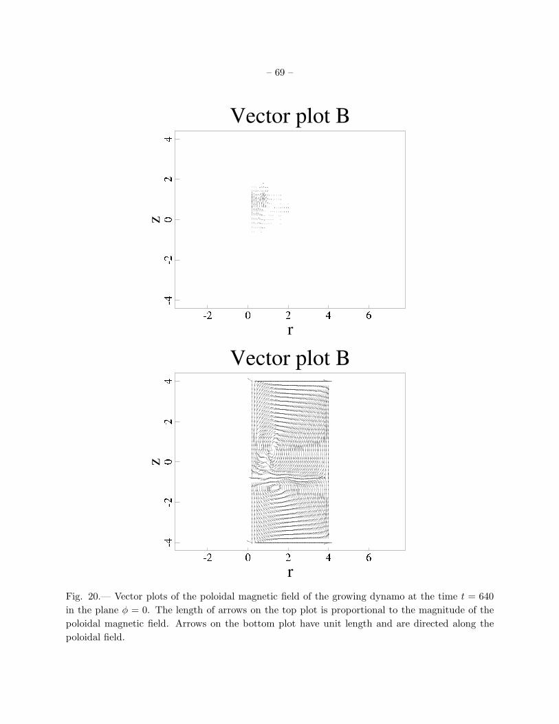
– 69 –

Fig. 20.— Vector plots of the poloidal magnetic field of the growing dynamo at the time t = 640

in the plane φ = 0. The length of arrows on the top plot is proportional to the magnitude of the

poloidal magnetic field. Arrows on the bottom plot have unit length and are directed along the

poloidal field.

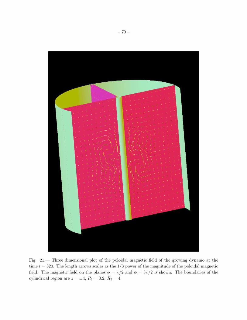
– 70 –

Fig. 21.— Three dimensional plot of the poloidal magnetic field of the growing dynamo at the

time t = 320. The length arrows scales as the 1/3 power of the magnitude of the poloidal magnetic

field. The magnetic field on the planes φ = π/2 and φ = 3π/2 is shown. The boundaries of the

cylindrical region are z = ±4, R1 = 0.2, R2 = 4.