A KRYLOV SUBSPACE ALGORITHM FOR EVALUATING THE … · A KRYLOV SUBSPACE ALGORITHM FOR EVALUATING...
21
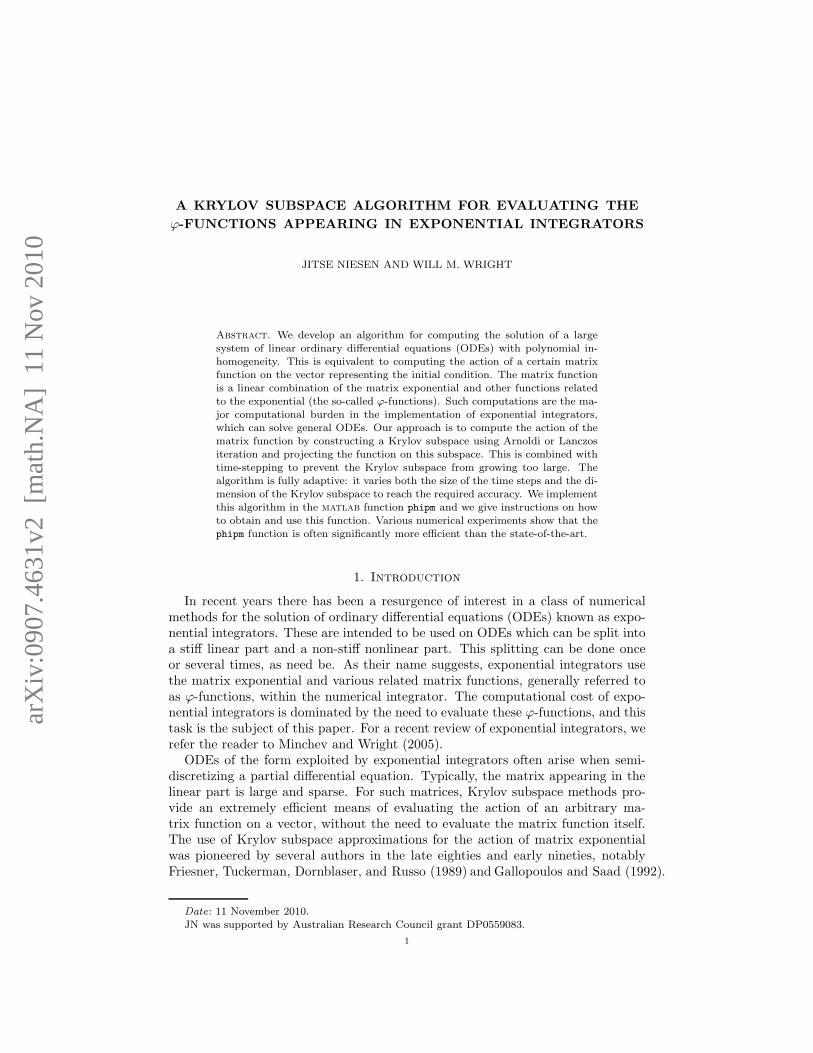
arXiv:0907.4631v2 [math.NA] 11 Nov 2010 A KRYLOV SUBSPACE ALGORITHM FOR EVALUATING THE ϕ-FUNCTIONS APPEARING IN EXPONENTIAL INTEGRATORS JITSE NIESEN AND WILL M. WRIGHT Abstract. We develop an algorithm for computing the solution of a large system of linear ordinary differential equations (ODEs) with polynomial in- homogeneity. This is equivalent to computing the action of a certain matrix function on the vector representing the initial condition. The matrix function is a linear combination of the matrix exponential and other functions related to the exponential (the so-called ϕ-functions). Such computations are the ma- jor computational burden in the implementation of exponential integrators, which can solve general ODEs. Our approach is to compute the action of the matrix function by constructing a Krylov subspace using Arnoldi or Lanczos iteration and projecting the function on this subspace. This is combined with time-stepping to prevent the Krylov subspace from growing too large. The algorithm is fully adaptive: it varies both the size of the time steps and the di- mension of the Krylov subspace to reach the required accuracy. We implement this algorithm in the matlab function phipm and we give instructions on how to obtain and use this function. Various numerical experiments show that the phipm function is often significantly more efficient than the state-of-the-art. 1. Introduction In recent years there has been a resurgence of interest in a class of numerical methods for the solution of ordinary differential equations (ODEs) known as expo- nential integrators. These are intended to be used on ODEs which can be split into a stiff linear part and a non-stiff nonlinear part. This splitting can be done once or several times, as need be. As their name suggests, exponential integrators use the matrix exponential and various related matrix functions, generally referred to as ϕ-functions, within the numerical integrator. The computational cost of expo- nential integrators is dominated by the need to evaluate these ϕ-functions, and this task is the subject of this paper. For a recent review of exponential integrators, we refer the reader to Minchev and Wright (2005). ODEs of the form exploited by exponential integrators often arise when semi- discretizing a partial differential equation. Typically, the matrix appearing in the linear part is large and sparse. For such matrices, Krylov subspace methods pro- vide an extremely efficient means of evaluating the action of an arbitrary ma- trix function on a vector, without the need to evaluate the matrix function itself. The use of Krylov subspace approximations for the action of matrix exponential was pioneered by several authors in the late eighties and early nineties, notably Friesner, Tuckerman, Dornblaser, and Russo (1989) and Gallopoulos and Saad (1992). Date : 11 November 2010. JN was supported by Australian Research Council grant DP0559083. 1
Transcript of A KRYLOV SUBSPACE ALGORITHM FOR EVALUATING THE … · A KRYLOV SUBSPACE ALGORITHM FOR EVALUATING...
arX
iv:0
907.
4631
v2 [
mat
h.N
A]
11
Nov
201
0
A KRYLOV SUBSPACE ALGORITHM FOR EVALUATING THE
ϕ-FUNCTIONS APPEARING IN EXPONENTIAL INTEGRATORS
JITSE NIESEN AND WILL M. WRIGHT
Abstract. We develop an algorithm for computing the solution of a largesystem of linear ordinary differential equations (ODEs) with polynomial in-homogeneity. This is equivalent to computing the action of a certain matrixfunction on the vector representing the initial condition. The matrix functionis a linear combination of the matrix exponential and other functions relatedto the exponential (the so-called ϕ-functions). Such computations are the ma-jor computational burden in the implementation of exponential integrators,which can solve general ODEs. Our approach is to compute the action of thematrix function by constructing a Krylov subspace using Arnoldi or Lanczositeration and projecting the function on this subspace. This is combined withtime-stepping to prevent the Krylov subspace from growing too large. Thealgorithm is fully adaptive: it varies both the size of the time steps and the di-mension of the Krylov subspace to reach the required accuracy. We implementthis algorithm in the matlab function phipm and we give instructions on howto obtain and use this function. Various numerical experiments show that thephipm function is often significantly more efficient than the state-of-the-art.
1. Introduction
In recent years there has been a resurgence of interest in a class of numericalmethods for the solution of ordinary differential equations (ODEs) known as expo-nential integrators. These are intended to be used on ODEs which can be split intoa stiff linear part and a non-stiff nonlinear part. This splitting can be done onceor several times, as need be. As their name suggests, exponential integrators usethe matrix exponential and various related matrix functions, generally referred toas ϕ-functions, within the numerical integrator. The computational cost of expo-nential integrators is dominated by the need to evaluate these ϕ-functions, and thistask is the subject of this paper. For a recent review of exponential integrators, werefer the reader to Minchev and Wright (2005).
ODEs of the form exploited by exponential integrators often arise when semi-discretizing a partial differential equation. Typically, the matrix appearing in thelinear part is large and sparse. For such matrices, Krylov subspace methods pro-vide an extremely efficient means of evaluating the action of an arbitrary ma-trix function on a vector, without the need to evaluate the matrix function itself.The use of Krylov subspace approximations for the action of matrix exponentialwas pioneered by several authors in the late eighties and early nineties, notablyFriesner, Tuckerman, Dornblaser, and Russo (1989) and Gallopoulos and Saad (1992).
Date: 11 November 2010.JN was supported by Australian Research Council grant DP0559083.
1
2 Jitse Niesen and Will M. Wright
Hochbruck and Lubich (1997) show that for particular classes of matrices, the con-vergence of the action of the matrix exponential on a vector is faster than thatfor the solution of the corresponding linear system. This suggests that exponentialintegrators can be faster than implicit methods, because computing the action ofthe matrix exponential and solving linear systems are the two fundamental opera-tions for exponential integrators and implicit methods, respectively. This analysisbreathed life back in the class of exponential integrators invented in the early six-ties, which had been abandoned in the eighties due to their excessive computationalexpense.
In their well-known paper on computing the matrix exponential, Moler and Van Loan (2003)write: “The most extensive software for computing the matrix exponential that weare aware of is expokit.” This refers to the work of Sidje (1998), who wrotesoftware for the computation of the matrix exponential of both small dense andlarge sparse matrices. The software uses a Krylov subspace approach in the largesparse setting. Computing the action of the matrix exponential is equivalentto solving a linear ODE, and Sidje uses this equivalence to apply time-steppingideas from numerical ODE methods in expokit. The time-steps are chosen withthe help of an error estimate due to Saad (1992). Sidje (1998) extends this ap-proach to the computation of the first ϕ-function, which appears in the solu-tions of linear ODEs with constant inhomogeneity. This was further generalizedby Sofroniou and Spaletta (2007) to polynomial inhomogeneities (or, from anotherpoint of view, to general ϕ-functions); their work is included in the latest versionof mathematica.
In all the approaches described above the size of the Krylov subspace is fixed,generally to thirty. Hochbruck, Lubich, and Selhofer (1998) explain in their land-mark paper one approach to adapt the size of the Krylov subspace. In this paper,we develop a solver which combines the time-stepping ideas of Sidje (1998) andSofroniou and Spaletta (2007) with the adaptivity of the dimension of the Krylovsubspace as described by Hochbruck, Lubich, and Selhofer (1998). We do not ex-amine the case of small dense matrices; this has been studied by Koikari (2007) andSkaflestad and Wright (2009). This algorithm described in this paper can be usedas a kernel for the efficient implementation of certain classes of exponential inte-grators. We also recommend the recent book by Higham (2008), which discussesmany of the issues related to matrix functions and their computation.
The approach followed in this paper, reducing large matrices to smaller onesby projecting them on Krylov subspace, is not the only game in town. Otherpossibilities are restricted-denominator rational Krylov methods (Moret 2007), thereal Leja point method (Caliari and Ostermann 2009), quadrature formulas basedon numerical inversion of sectorial Laplace transforms (Lopez-Fernandez 2010), andcontour integration (Schmelzer and Trefethen 2007). These methods are outsidethe scope of this paper, but we intend to study and compare them in future work.
The outline of this paper follows. In Section 2 we present several useful resultsregarding the ϕ-functions. The algorithm we have developed is explained in Sec-tion 3, where we present the Krylov subspace method, show how error estimation,time-stepping and adaptivity are handled in our algorithm, and finally give someinstructions on how to use our implementation. Several numerical experiments aregiven in Section 4 followed by some concluding remarks and pointers towards futurework in Section 5.
A Krylov subspace algorithm for evaluating the ϕ-functions 3
2. The ϕ-functions
Central to the implementation of exponential integrators is the efficient andaccurate evaluation of the matrix exponential and other ϕ-functions. These ϕ-functions are defined for scalar arguments by the integral representation
(1) ϕ0(z) = ez, ϕℓ(z) =1
(ℓ− 1)!
∫ 1
0
e(1−θ)zθℓ−1 dθ, ℓ = 1, 2, . . . , z ∈ C.
For small values of ℓ, these functions are
ϕ1(z) =ez − 1
z, ϕ2(z) =
ez − 1− z
z2, ϕ3(z) =
ez − 1− z − 12z
2
z3.
The ϕ-functions satisfy the recurrence relation
(2) ϕℓ(z) = zϕℓ+1(z) +1
ℓ!, ℓ = 1, 2, . . . .
The definition can then be extended to matrices instead of scalars using any of theavailable definitions of matrix functions, such as that based on the Jordan canonicalform (Horn and Johnson 1991; Higham 2008).
Every stage in an exponential integrator can be expressed as a linear combinationof ϕ-functions acting on certain vectors:
(3) ϕ0(A)b0 + ϕ1(A)b1 + ϕ2(A)b2 + · · ·+ ϕp(A)bp.
Here p is related to the order of the exponential integrator, typically taking valuesless than five. A is a matrix, often the Jacobian for exponential Rosenbrock-typemethods or an approximation to it for methods based on the classical linear/non-linear splitting; usually, A is large and sparse.
We need to compute expressions of the form (3) several times in each step thatthe integrator takes, so there is a need to evaluate these expressions efficiently andaccurately. This is the problem taken up in this paper. We would like to stress thatany procedure for evaluating (3), such as the one described here, is independentof the specific exponential integrator used and can thus be re-used in differentintegrators. The exponential integrators differ in the vectors b0, . . . , bp appearingin (3).
The following lemma gives a formula for the exact solution of linear differentialequations with polynomial inhomogeneity. This result partly explains the importantrole that ϕ-functions play in exponential integrators (see Minchev and Wright (2005)for more details). The lemma also provides the background for the time-steppingprocedure for the evaluation of (3) which we develop in §3.3.Lemma 2.1 ((Skaflestad and Wright (2009))). The solution of the non-autonomous
linear initial value problem
(4) u′(t) = Au(t) +
p−1∑
j=0
tj
j!bj+1, u(tk) = uk,
is given by
u(tk + τk) = ϕ0(τkA)uk +
p−1∑
j=0
j∑
ℓ=0
tj−ℓk
(j − ℓ)!τ ℓ+1k ϕℓ+1(τkA)bj+1,
where the functions ϕℓ are defined in (1).
4 Jitse Niesen and Will M. Wright
Proof. Recall that ϕ0 denotes the matrix exponential. Using ϕ0((tk − t)A) as anintegrating factor for (4) we arrive at
u(tk + τk) = ϕ0(τkA)uk + ϕ0(τkA)
∫ τk
0
ϕ0(−sA)
p−1∑
j=0
(tk + τk)j
j!bj+1 ds
= ϕ0(τkA)uk + ϕ0(τkA)
∫ τk
0
ϕ0(−sA)
p−1∑
j=0
j∑
ℓ=0
tj−ℓk sℓ
ℓ!(j − ℓ)!bj+1 ds.
Now change the integration variable, s = θτk, and apply the definition (1) of theϕ-functions.
= ϕ0(τkA)uk +
d−1∑
j=0
j∑
ℓ=0
tj−ℓk
(j − ℓ)!τ ℓ+1k
(
1
ℓ!
∫ 1
0
ϕ0((1 − θ)τkA)θℓ dθ
)
bj+1
= ϕ0(τkA)uk +
p−1∑
j=0
j∑
ℓ=0
tj−ℓk
(j − ℓ)!τ ℓ+1k ϕℓ+1(τkA)bj+1.
�
3. The algorithm
This section describes the details of our algorithm for evaluating expressionsof the form (3) as implemented in the matlab function phipm. In the first partof this section we explain how Krylov subspace techniques can be used to reducelarge matrices to small ones when evaluating matrix functions. An estimate of theerror committed in the Krylov subspace approximation is essential for an adaptivesolver; this is dealt with in the second part. Then we discuss how to split up thecomputation of the ϕ-functions into several steps. Part four concerns the possibilityof adapting the Krylov subspace dimension and the size of the steps using the errorestimate from the second part, and the interaction between both forms of adaptivity.Finally, we explain how to use the implementation provided in the phipm function.
3.1. The basic method. We start by considering how to compute ϕp(A)v, whereA is an n × n matrix (with n large) and v ∈ Rn. This is one of the terms in (3).We will use a Krylov subspace approach for this task.
The idea behind this Krylov subspace approach is quite simple. The vectorϕp(A)v lives in Rn, which is a big space. We approximate it in a smaller space ofdimension m. This smaller space is the Krylov subspace, which is given by
Km = span{v,Av,A2v, . . . , Am−1v}.However, the vectors Ajv form a bad basis for the Krylov subspace because theypoint in almost the same direction as the dominant eigenvector of A; thus, the basisvectors are almost linearly dependent. In fact, computing these successive productsis the power iteration method for evaluating the dominant eigenvector. Therefore,we apply the (stabilized) Gram–Schmidt procedure to get an orthonormal basis ofthe Krylov subspace:
Km = span{v1, v2, . . . , vm}.Let Vm denote the n-by-m matrix whose columns are v1, . . . , vm. Then the m-by-mmatrix Hm = V T
mAVm is the projection of the action of A to the Krylov subspace,
A Krylov subspace algorithm for evaluating the ϕ-functions 5
expressed in the basis {v1, . . . , vm}. The Arnoldi iteration (Algorithm 1) computesthe matrices Hm and Vm, see Saad (1992).
Algorithm 1 The Arnoldi iteration.
v1 = v/‖v‖for j = 1, . . . ,m do
w = Avjfor i = 1, . . . , j do
hi,j = vTi w; w = w − hi,jviend for
hj+1,j = ‖w‖; vj+1 = w/hj+1,j
end for
It costs 32 (m
2 − m + 1)n floating point operations (flops) and m products ofA with a vector to compute the matrices Hm and Vm. The cost of one of thesematrix-vector products depends on the sparsity of A; the straightforward approachuses 2NA flops where NA is the number of nonzero entries in the matrix A.
The projection of the action of A on the Krylov subspace Km in the standardbasis of Rn is VmHmV T
m . We now approximate ϕp(A)v by ϕp(VmHmV Tm )v. Since
V TmVm = Im and VmV T
m v = v we have ϕp(VmHmV Tm )v = Vmϕp(Hm)V T
m v. Finally,V Tm v = ‖v‖e1, where e1 is the first vector in the standard basis. Taking everything
together, we arrive at the approximation
(5) ϕp(A)v ≈ βVmϕp(Hm)e1, β = ‖v‖.The advantage of this formulation is that the matrix Hm has size m-by-m and thusit is much cheaper to evaluate ϕp(Hm) than ϕp(A).
The matrix Hm is Hessenberg, meaning that the (i, j) entry vanishes wheneveri > j + 1. It is related to the matrix A by the relation Hm = V T
mAVm. If Ais symmetric, then Hm is both symmetric and Hessenberg, which means that itis tridiagonal. In that case, we denote the matrix by Tm, and we only need tra-verse the i-loop in the Arnoldi iteration twice: once for i = j − 1 and once fori = j. The resulting algorithm is known as the Lanczos iteration (Algorithm 2);see Trefethen and Bau (1997, Alg 36.1). It takes 3(2m− 1)n flops and m productsof A with a vector to compute Tm and Vm when A is symmetric.
Algorithm 2 The Lanczos iteration.
t1,0 = 0; v0 = 0; v1 = v/‖v‖for j = 1, . . . ,m do
w = Avj ; tj,j = vTj ww = w − tj,j−1vj−1 − tj,jvjtj,j−1 = ‖w‖; tj−1,j = ‖w‖vj+1 = w/tj,j−1
end for
The Krylov subspace algorithm reduces the problem of computing ϕp(A)v whereA is a big n-by-n matrix to that of computing ϕp(Hm)e1 where Hm is a smallerm-by-m matrix. Skaflestad and Wright (2009) describe a modified scaling-and-squaring method for the computation of ϕp(Hm). However, this method has the
6 Jitse Niesen and Will M. Wright
disadvantage that one generally also has to compute ϕ0(Hm), . . . , ϕp−1(Hm). It is
usually cheaper to compute the matrix exponential exp(Hm) of a slightly larger ma-
trix Hm, following an idea of Saad (1992, Prop. 2.1), generalized by Sidje (1998, Thm. 1)
to p > 1. Indeed, if we define the augmented matrix Hm by
(6) Hm =
Hm e1 0 m rows0 0 I p− 1 rows0 0 0 1 row
then the top m entries of the last column of exp(Hm) yield the vector ϕp(Hm)e1.
Finally, we compute the matrix exponential exp(Hm) using the degree-13 diagonalPade approximant combined with scaling and squaring as advocated by Higham (2005);this is the method implemented in the function expm in matlab Version 7.2 (R2006a)and later. In contrast, expokit uses the degree-14 uniform rational Chebyshev ap-proximant for symmetric negative-definite matrices and the degree-6 diagonal Padeapproximant for general matrices, combined with scaling and squaring. We choosenot to deal with the negative-definite matrices separately, but consider this as apossible extension to consider at a later date. Koikari (2009) recently developed anew variant of the Schur–Parlett algorithm using three-by-three blocking.
The computation of exp(Hm) using Higham’s method requires one matrix divi-
sion (costing 83 (m+ p)3 flops) and 6+ ⌈log2(‖Hm‖1/5.37)⌉+ matrix multiplications
(costing 2(m+p)3 flops each), where ⌈x⌉+ denotes the smallest nonnegative integer
larger than x. Thus, the total cost of computing the matrix exponential of Hm is
M(Hm) (m+ p)3 where
(7) M(A) =44
3+ 2
⌈
log2‖A‖15.37
⌉
+
.
Only the last column of the matrix exponential exp(Hm) is needed; it is naturalto ask if this can be exploited. Alternatively one could ask whether the computa-tion of exp(Hm) using the scaling-and-squaring algorithm can be modified to take
advantage of the fact that Hm is Hessenberg (Higham (2008, Prob. 13.6) suggeststhis as a research problem). The algorithm suggested by Higham (2005, Alg. 2.3)computes the matrix exponential to machine precision (Higham considers IEEEsingle, double and quadruple precision). The choice of the degree of the Padeapproximation and the number of scaling steps is intimately connected with thischoice of precision. However, we generally do not require this accuracy. It would beinteresting to see if significant computational savings can be gained in computingthe matrix exponential by developing an algorithm with several other choices ofprecision.
3.2. Error estimation. Saad (1992, Thm. 5.1) derives a formula for the error inthe Krylov subspace approximation (5) to ϕp(A)v in the case p = 0. This resultwas generalized by Sidje (1998, Thm. 2) to p > 0. Their result states that
(8) ϕp(A)v − βVmϕp(Hm)e1 = β
∞∑
j=p+1
hm+1,meTmϕj(Hm)e1Aj−p−1vm+1.
The first term in the series on the right-hand side does not involve any multiplica-tions with the matrix A and the Arnoldi iteration already computes vector vm+1,
A Krylov subspace algorithm for evaluating the ϕ-functions 7
so this term can be computed without too much effort. We use this term as anerror estimate for the approximation (5):
(9) ε = ‖βhm+1,meTmϕp+1(Hm)e1vm+1‖ = β|hm+1,m| [ϕp+1(Hm)]m,1.
Further justification for this error estimate is given by Hochbruck, Lubich, and Selhofer (1998).We also use this error estimate as a corrector: instead of (5), we use
(10) ϕp(A)v ≈ βVmϕp(Hm)e1 + βhm+1,meTmϕp+1(Hm)e1vm+1.
If ϕp+1(Hm)e1 is computed using the augmented matrix (6), then ϕp(Hm)e1 alsoappears in the result, so we only need to exponentiate a matrix of size m+ p+ 1.The approximation (10) is more accurate, but ε is no longer a real error estimate.This is acceptable because, as explained below, it is not used as an error estimatebut only for the purpose of adaptivity.
Sidje (1998) proposes a more accurate error estimate which also uses the secondterm of the series in (8). However, the computation of this requires a matrix-vectorproduct and the additional accuracy is in our experience limited. We thus do notuse Sidje’s error estimate.
3.3. Time-stepping. Saad (1992, Thm. 4.7) proves that the error of the approx-imation (5) satisfies the bound
(11) ‖Error‖ ≤ 2β(ρ(A))m
m!(1 + o(1))
for sufficiently large m, where ρ(A) denotes the spectral radius of A. This bounddeteriorates as ρ(A) increases, showing that the dimensionm of the Krylov subspacehas to be large if ρ(A) is large. Sidje (1998) proposes an alternative method forcomputing ϕ1(A)v when ρ(A) is large, based on time-stepping. This approach isgeneralized by Sofroniou and Spaletta (2007) for general ϕ-functions.
The main idea behind this time-stepping procedure is that ϕp(A)v solves a non-autonomous linear ODE. More generally, Lemma 2.1 states that the function
(12) u(t) = ϕ0(tA)b0 + tϕ1(tA)b1 + t2ϕ2(tA)b2 + · · ·+ tpϕp(tA)bp,
is the solution of the differential equation
(13) u′(t) = Au(t) + b1 + tb2 + · · ·+ tp−1
(p− 1)!bp, u(0) = b0.
We now use a time-stepping method to calculate u(tend) for some tend ∈ R. If wewant to compute an expression of the form (3), we set tend = 1. Split the timeinterval [0, tend] by introducing a grid 0 = t0 < t1 < . . . < tn = tend. To advancethe solution, say from tk to tk+1, we need to solve the differential equation (13)with the value of u(tk) as initial condition. The relation between u(tk) and u(tk+1)is given in Lemma 2.1. Rearranging this expression gives
(14) u(tk+1) = ϕ0(τkA)u(tk) +
p∑
i=1
τ ikϕi(τkA)
p−i∑
j=0
tjkj!bi+j ,
where τk = tk+1− tk. However, we do not need to evaluate all the ϕ-functions. Therecurrence relation ϕq(A) = ϕq+1(A)A+ 1
q! I implies that
ϕq(A) = ϕp(A)Ap−q +
p−q−1∑
j=0
1
(q + j)!Aj , q = 0, 1, . . . , p− 1.
8 Jitse Niesen and Will M. Wright
Substituting this in (14) yields
(15) u(tk+1) = τpkϕp(τkA)wp +
p−1∑
j=0
τ jkj!wj ,
where the vectors wj are given by
wj = Aju(tk) +
j∑
i=1
Aj−i
j−i∑
ℓ=0
tℓkℓ!bi+ℓ, j = 0, 1, . . . , p.
This is the time-stepping method for computing (3).The computational cost of this method is as follows. At every step, we need
to compute the vectors wj for j = 0, . . . , p, the action of ϕp(τkA) on a vector,p + 1 scalar multiplications of a vector of length n and p vector additions. Thevectors wj satisfy the recurrence relation
(16) w0 = u(tk) and wj = Awj−1 +
p−j∑
ℓ=0
tℓkℓ!bj+ℓ, j = 1, . . . , p,
and hence their computation requires p multiplications of A with a vector, p scalarmultiplications, and p vector additions.
One reason for developing this time-stepping method is to reduce the dimensionof the Krylov subspace. If the spectrum of A is very large, multiple time-stepsmay be required. We intend, in the future, to compare this approach with theapproach described by Skaflestad and Wright (2009) which evaluates the matricesϕ0(Hm), . . . , ϕp+1(Hm) directly. The latter method may have computational ad-vantages, particularly if b0, . . . , bp are equal or zero. For values of p that we areinterested in, that is less than five, we have not noticed any loss of accuracy usingthis approach. We intend to look into this issue more thoroughly in future investiga-tions, especially in light of the paper (Al-Mohy and Higham 2010), which appearedduring the review process, which noticed that for large values of p accuracy can belost.
We choose an initial step size similar to the one suggested in expokit, exceptwe increase the rather conservative estimate by an order of magnitude, to give
(17) τ0 =10
‖A‖∞
(
Tol(
(mave + 1)/e)mave+1√
2π(mave + 1)
4‖A‖∞‖b0‖∞
)1/mave
,
where Tol is the user defined tolerance and mave is the average of the input andmaximum allowed size of the Krylov subspace.
3.4. Adaptivity. The procedure described above has two key parameters, the di-mension m of the Krylov subspace and the time-step τ . These need to be chosenappropriately. As we cannot expect the user to make this choice, and the optimalvalues may change, the algorithm needs to determine m and τ adaptively.
We are using a time-stepping method, so adapting the step size τ is similar toadaptivity in ODE solvers. This has been studied extensively. It is described byButcher (2008, §39) and Hairer, Nørsett, and Wanner (1993, §II.4), among others.The basic idea is as follows. We assume that the time-stepping method has or-der q, so that the error is approximately Cτq+1 for some constant C. We somehow
A Krylov subspace algorithm for evaluating the ϕ-functions 9
compute an error estimate ε and choose a tolerance Tol that the algorithm shouldsatisfy. Then the optimal choice for the new step size is
(18) τnew = τk
(
1
ω
)1/(q+1)
where ω =tend‖ε‖τk · Tol .
The factor tend is included so that the method is invariant under time scalings.Usually, a safety factor γ is added to ensure that the error will probably satisfy theerror tolerance, changing the formula to τnew = τk(γ/ω)
1/(q+1). Common choicesare γ = 0.25 and γ = 0.38. However, in our case the consequence of rejecting astep is that we computed the matrix exponential in vain, while in ODE solvers thewhole computation has to be repeated when a step is rejected. We may thus bemore adventurous and therefore we take γ = 0.8.
In our scheme, the error estimate ε is given by (9). However, what is the order qfor our scheme? The a priori estimate (11) suggests that the order equals thedimension m of the Krylov subspace. Experiments confirm that the error is indeedproportional to τm+1 in the limit τ → 0. However, for finite step size the error isbetter described by τq with a smaller exponent q. Let us call the exponent q whichprovides the best fit around a given value step size τ the “heuristic order”, for lackof a better term.
We can estimate the heuristic order if we have attempted two step sizes duringthe same step, which happens if we have just rejected a step and reduced the stepsize. The estimate for the heuristic order is then
(19) q =log(τ/τold)
log(‖ε‖/‖εold‖)− 1,
where ε and εold denote the error estimates produced when attempting step size τand τold, respectively. In all other cases, we use q = 1
4m; there is no rigorous
argument behind the choice of 14 but it seems to yield good performance in practice.
With this estimate for the heuristic order, we compute the suggested new stepsize as
(20) τnew = τk
( γ
ω
)1/(q+1)
.
The other parameter that we want to adapt is the Krylov subspace dimension m.The error bound (11) suggests that, at least for modest changes of m, the error isapproximately equal to Cκ−m for some values of C and k. Again, we can estimateκ if we have error estimates corresponding to two different values of m:
(21) κ =
( ‖ε‖‖εold‖
)1/(mold−m)
.
If this formula cannot be used, then we take κ = 2. Given this estimate, theminimal m which satisfies the required tolerance is given by
(22) mnew = m+log(ω/γ)
log κ.
We now have to choose between two possibilities: either we keep m constant andchange τ to τnew, or we keep τ constant and change m to mnew. We will pick thecheapest option. To advance from tk to tk+1, we need to evaluate (15). Computa-tion of the vectors wj requires 2(p− 1)(NA+n) flops. Then, we need to do m steps
10 Jitse Niesen and Will M. Wright
of the Arnoldi algorithm, for a cost of 32 (m
2 −m+1)n+ 2mNA flops. If A is sym-metric, we will use the Lanczos algorithm and the costs drops to 3(2m−1)n+2mNA
flops. To compute ϕp(τkA)wp in (15) using (10), we need to exponentiate a matrix
of size m + p + 1, costing M(Hm) (m + p + 1)3 flops with M(Hm) given by (7).Finally, the scalar multiplications and vector additions in (15) requires a further(2p+ 1)n flops. All together, we find that the cost of a single step is(23)
C1(m) =
{
(m+ p)NA + 3(m+ p)n+M(Hm) (m+ p+ 1)3, for Lanczos;
(m+ p)NA + (m2 + 3p+ 2)n+M(Hm) (m+ p+ 1)3, for Arnoldi.
This needs to be multiplied with the number of steps required to go from the currenttime tk to the end point t = tend. So the total cost is
(24) C(τ,m) =
⌈
tend − tkτ
⌉
C1(m).
We compute C(τnew,m) and C(τ,mnew) according to this formula. If C(τnew,m) issmaller, then we change the time-step to τnew and leave m unchanged. However, toprevent too large changes in τ we restrict it to change by no more than a factor 5.Similarly, if C(τnew,m) is smaller, then τ remains as it is and we change m to mnew,except that we restrict it to change by no more as a factor 4
3 (this factor is chosenfollowing Hochbruck, Lubich, and Selhofer (1998)).
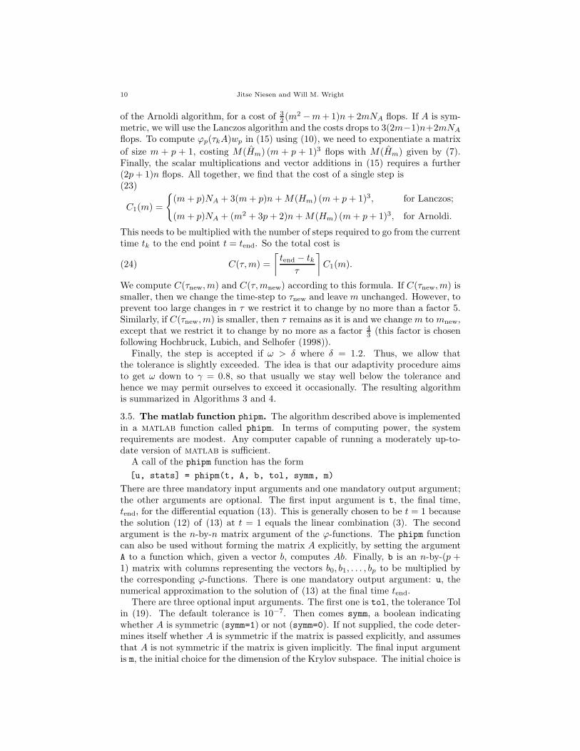
Finally, the step is accepted if ω > δ where δ = 1.2. Thus, we allow thatthe tolerance is slightly exceeded. The idea is that our adaptivity procedure aimsto get ω down to γ = 0.8, so that usually we stay well below the tolerance andhence we may permit ourselves to exceed it occasionally. The resulting algorithmis summarized in Algorithms 3 and 4.
3.5. The matlab function phipm. The algorithm described above is implementedin a matlab function called phipm. In terms of computing power, the systemrequirements are modest. Any computer capable of running a moderately up-to-date version of matlab is sufficient.
A call of the phipm function has the form
[u, stats] = phipm(t, A, b, tol, symm, m)
There are three mandatory input arguments and one mandatory output argument;the other arguments are optional. The first input argument is t, the final time,tend, for the differential equation (13). This is generally chosen to be t = 1 becausethe solution (12) of (13) at t = 1 equals the linear combination (3). The secondargument is the n-by-n matrix argument of the ϕ-functions. The phipm functioncan also be used without forming the matrix A explicitly, by setting the argumentA to a function which, given a vector b, computes Ab. Finally, b is an n-by-(p +1) matrix with columns representing the vectors b0, b1, . . . , bp to be multiplied bythe corresponding ϕ-functions. There is one mandatory output argument: u, thenumerical approximation to the solution of (13) at the final time tend.
There are three optional input arguments. The first one is tol, the tolerance Tolin (19). The default tolerance is 10−7. Then comes symm, a boolean indicatingwhether A is symmetric (symm=1) or not (symm=0). If not supplied, the code deter-mines itself whether A is symmetric if the matrix is passed explicitly, and assumesthat A is not symmetric if the matrix is given implicitly. The final input argumentis m, the initial choice for the dimension of the Krylov subspace. The initial choice is
A Krylov subspace algorithm for evaluating the ϕ-functions 11
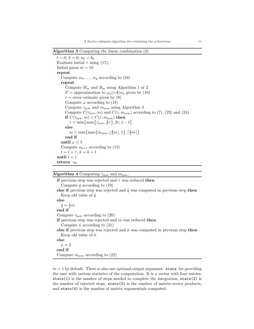
Algorithm 3 Computing the linear combination (3).
t = 0; k = 0; uk = b0Evaluate initial τ using (17);Initial guess m = 10repeat
Compute w0, . . . , wp according to (16)repeat
Compute Hm and Bm using Algorithm 1 or 2F = approximation to ϕp(τA)wp given by (10)ε = error estimate given by (9)Compute ω according to (18)Compute τnew and mnew using Algorithm 4Compute C(τnew,m) and C(τ,mnew) according to (7), (23) and (24)if C(τnew,m) < C(τ,mnew) thenτ = min
{
max{
τnew,15τ}
, 2τ, 1− t}
else
m = min{
max{
mnew, ⌊ 34m⌋, 1
}
, ⌈ 43m⌉
}
end if
until ω ≤ δCompute uk+1 according to (15)t = t+ τ ; k = k + 1
until t = 1return uk
Algorithm 4 Computing τnew and mnew.
if previous step was rejected and τ was reduced then
Compute q according to (19)else if previous step was rejected and q was computed in previous step then
Keep old value of qelse
q = 14m
end if
Compute τnew according to (20)if previous step was rejected and m was reduced then
Compute κ according to (21)else if previous step was rejected and κ was computed in previous step then
Keep old value of κelse
κ = 2end if
Compute mnew according to (22)
m = 1 by default. There is also one optional output argument: stats, for providingthe user with various statistics of the computation. It is a vector with four entries:stats(1) is the number of steps needed to complete the integration, stats(2) isthe number of rejected steps, stats(3) is the number of matrix-vector products,and stats(4) is the number of matrix exponentials computed.
12 Jitse Niesen and Will M. Wright
4. Numerical experiments
In this section we perform several numerical experiments, which illustrate theadvantages of the approach that has been outlined in the previous sections. Wecompare the function phipm with various state-of-the-art numerical algorithms.The first experiment compares several numerical ODE solvers on a large systemof linear ODEs, resulting from the finite-difference discretization of the HestonPDE, a common example from the mathematical finance literature. The secondexperiment compares our function phipm and the expv and phiv functions fromexpokit on various large sparse matrices. This repeats the experiment reportedby Sidje (1998).
All experiments use a MacBookPro with 2.66 GHz Intel Core 2 Duo processor and4GB 1067 MHz DDR3 memory. We use matlab Version 7.11 (R2010b) for all ex-periments, which computes the matrix exponential as described in Higham (2005).We have noticed that the results described in this section depend on the specifica-tions of the computer but the overall nature of the numerical experiments remainsthe same.
4.1. The Heston equation in financial mathematics. A European call optiongives its owner the right (but not obligation) to buy a certain asset for a certainprice (called the strike price) at a certain time (the expiration date). European calloptions with stochastic volatility, modeled by a stochastic mean-reverting differen-tial equation, have been successfully priced by Heston (1993). The Heston pricingformulae are a natural extension of the celebrated Black–Scholes–Merton pricingformulae. Despite the existence of a semi-closed form solution, which requires thenumerical computation of an indefinite integral, the so-called Heston PDE is oftenused as a test example to compare various numerical integrators. This examplefollows closely In ’t Hout (2007) and In ’t Hout and Foulon (2010).
Let U(s, v, t) denote the European call option price at time T − t, where s isthe price of the underlying asset and v the variance in the asset price at thattime. Here, T is the expiration date of the option. Heston’s stochastic volatilitymodel ensures that the price of a European call option satisfies the time-dependentconvection-diffusion-reaction equation
Ut =1
2vs2Uss + ρλvsUvs +
1
2λ2vUvv + (rd − rf )sUs + κ(η − v)Uv − rdU.
This equation is posed on the unbounded spatial domain s > 0 and v ≥ 0, while tranges from 0 to T . Here, ρ ∈ [−1, 1] represents the correlation between the Wienerprocesses modeling the asset price and its variance, λ is a positive scaling constant,rd and rf are constants representing the risk-neutral domestic and foreign interestrates respectively, η represents the mean level of v and κ the rate at which v revertsto η. The payoff of the European call option provides the initial condition
U(s, v, 0) = max(s−K, 0),
where K ≥ 0 denotes the strike price.The unbounded spatial domain must be restricted in size in computations and
we choose the sufficiently large rectangle [0, S]× [0, V ]. Usually S and V are chosenmuch larger than the values of s and v of practical interest. This is a commonlyused approach in financial modeling so that if the boundary conditions are im-perfect their effect is minimized, see Tavella and Randall (2000, p. 121). Suitable
A Krylov subspace algorithm for evaluating the ϕ-functions 13
boundary conditions for 0 < t ≤ T are
U(0, v, t) = 0,
U(s, V, t) = s,
Us(S, v, t) = 1,
Ut(s, 0, t)− (rd − rf )sUs(s, 0, t)− κηUv(s, 0, t) + rU(s, 0, t) = 0.
Note that the boundary and initial conditions are inconsistent or non-matching,that is the boundary and initial conditions at t = 0 do not agree.
We discretize the spatial domain using a uniform rectangular mesh with meshlengths ∆s and ∆v and use standard second-order finite differences to approximatethe derivatives as follows:
(Us)i,j ≈Ui+1,j − Ui−1,j
2∆s,
(Uss)i,j ≈Ui+1,j − 2Ui,j + Ui−1,j
∆s2,
(Uv)i,j ≈Ui,j+1 − Ui,j−1
2∆v,
(Uv)i,0 ≈ −3Ui,0 + 4Ui,1 − Ui,2
2∆v,
(Uvv)i,j ≈Ui,j+1 − 2Ui,j + Ui,j−1
∆v2,
(Usv)i,j ≈Ui+1,j+1 + Ui−1,j−1 − Ui−1,j+1 − Ui+1,j−1
4∆v∆s.
The boundary associated to v = 0 is included in the mesh, but the other threeboundaries are not. Combining the finite-difference discretization and the boundaryconditions leads to a large system of ODEs of the form
u′(t) = Au(t) + b1, u(0) = b0.
The exact solution for this system is given in Lemma 2.1. This is a natural problemfor the phipm solver.
We compare five methods: the scheme of Crank and Nicolson (1947), two Al-ternating Direction Implicit (ADI) schemes, ode15s from matlab and the phipm
method described in this paper. The two ADI schemes are the method due toDouglas and Rachford (1956) with θ = 1
2 , and the method of Hundsdorfer and Verwer (2003)
with θ = 310 and µ = 1
2 . The first ADI method is of order one and the second methodis of order two. In ’t Hout (2007) lists each of the ADI methods described aboveand explains necessary implementation details; the stability of these methods isdiscussed in In ’t Hout and Welfert (2009). To compare phipm with an adaptivesolver we choose the in-built matlab solver ode15s, which is a variable step size,variable order implementation of the backward differentiation formulae (BDF). TheJacobian of the right-hand side (that is, the matrix A) is passed to ode15s; thismakes ode15s considerably faster.
We choose the same problem parameters as in the paper by (In ’t Hout 2007):namely κ = 2, ν = 0.2, λ = 0.3, ρ = 0.8, rd = 0.03, rf = 0.0, the optionmaturity T = 1 and the strike price K = 100. The spatial domain is truncated to[0, 8K]× [0, 5]. We use a grid with 100 points in the s-direction and 51 points inthe v-direction (recall that v = 0 is included in the grid and the other borders arenot). This results in a system with 5100 degrees of freedom, with nnz = 44, 800
14 Jitse Niesen and Will M. Wright
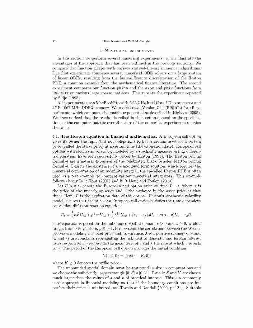
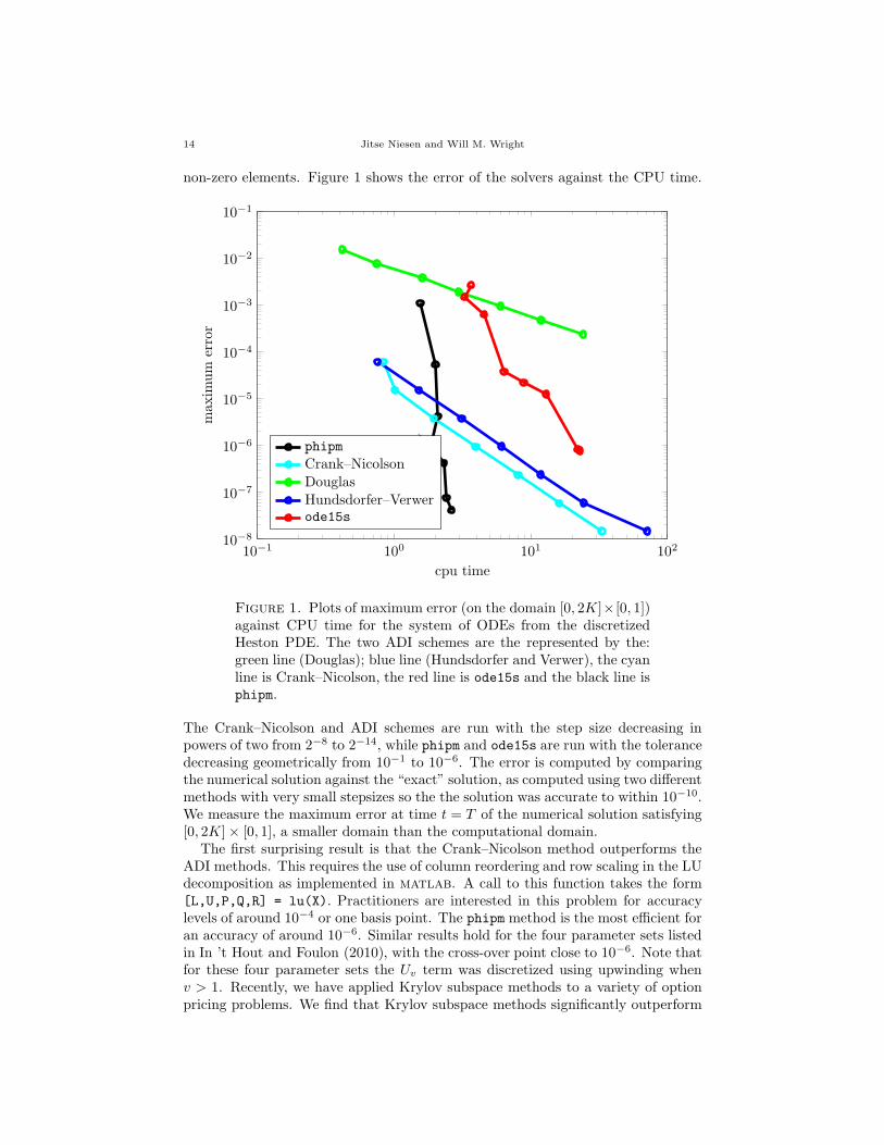
non-zero elements. Figure 1 shows the error of the solvers against the CPU time.
10−1 100 101 10210−8
10−7
10−6
10−5
10−4
10−3
10−2
10−1
cpu time
maxim
um
error
phipm
Crank–Nicolson
DouglasHundsdorfer–Verwerode15s
Figure 1. Plots of maximum error (on the domain [0, 2K]× [0, 1])against CPU time for the system of ODEs from the discretizedHeston PDE. The two ADI schemes are the represented by the:green line (Douglas); blue line (Hundsdorfer and Verwer), the cyanline is Crank–Nicolson, the red line is ode15s and the black line isphipm.
The Crank–Nicolson and ADI schemes are run with the step size decreasing inpowers of two from 2−8 to 2−14, while phipm and ode15s are run with the tolerancedecreasing geometrically from 10−1 to 10−6. The error is computed by comparingthe numerical solution against the “exact” solution, as computed using two differentmethods with very small stepsizes so the the solution was accurate to within 10−10.We measure the maximum error at time t = T of the numerical solution satisfying[0, 2K]× [0, 1], a smaller domain than the computational domain.
The first surprising result is that the Crank–Nicolson method outperforms theADI methods. This requires the use of column reordering and row scaling in the LUdecomposition as implemented in matlab. A call to this function takes the form[L,U,P,Q,R] = lu(X). Practitioners are interested in this problem for accuracylevels of around 10−4 or one basis point. The phipm method is the most efficient foran accuracy of around 10−6. Similar results hold for the four parameter sets listedin In ’t Hout and Foulon (2010), with the cross-over point close to 10−6. Note thatfor these four parameter sets the Uv term was discretized using upwinding whenv > 1. Recently, we have applied Krylov subspace methods to a variety of optionpricing problems. We find that Krylov subspace methods significantly outperform
A Krylov subspace algorithm for evaluating the ϕ-functions 15
0 5 · 10−2 0.1 0.15 0.2 0.25 0.3 0.35 0.430
32
34
36
38
40
m
0 5 · 10−2 0.1 0.15 0.2 0.25 0.3 0.35 0.42
2.5
3
3.5
4·10−3
t
τ
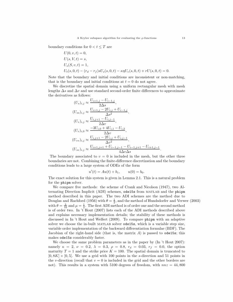
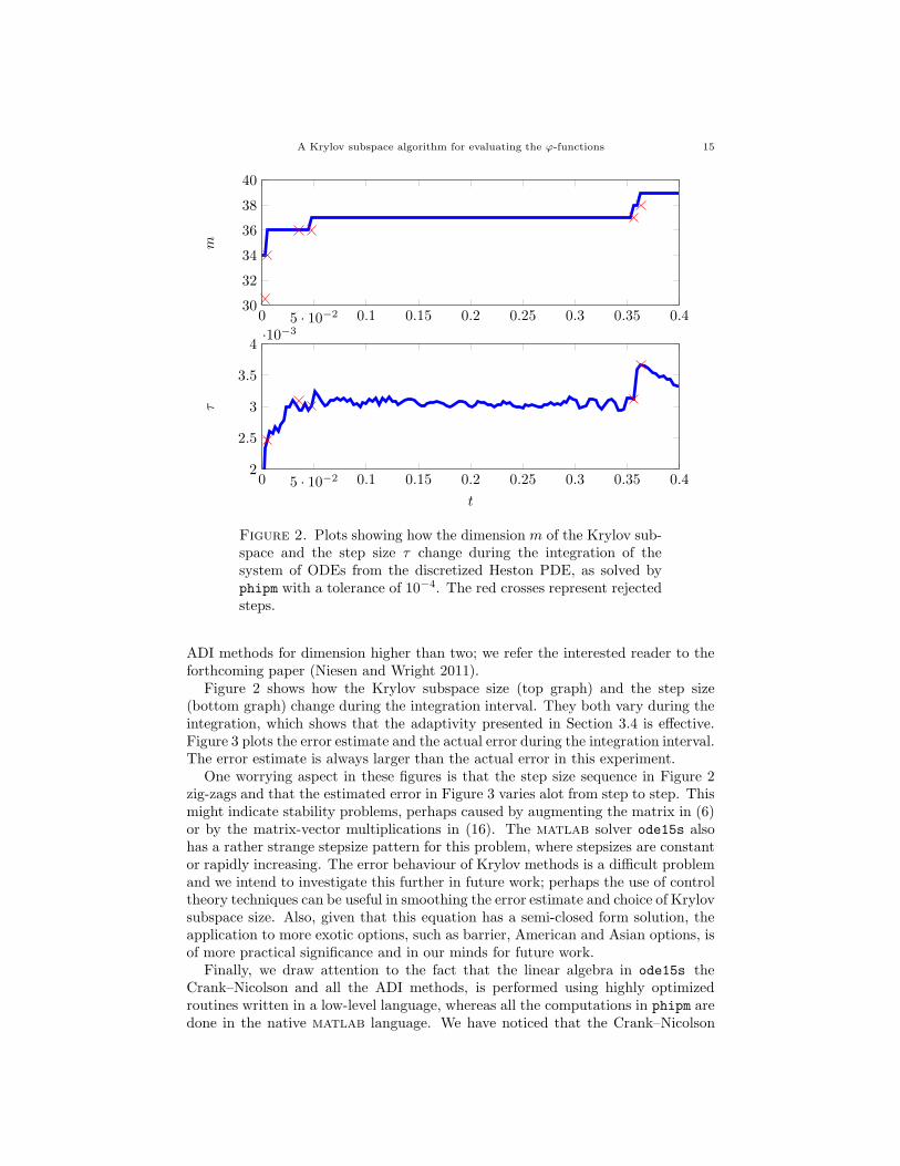
Figure 2. Plots showing how the dimension m of the Krylov sub-space and the step size τ change during the integration of thesystem of ODEs from the discretized Heston PDE, as solved byphipm with a tolerance of 10−4. The red crosses represent rejectedsteps.
ADI methods for dimension higher than two; we refer the interested reader to theforthcoming paper (Niesen and Wright 2011).
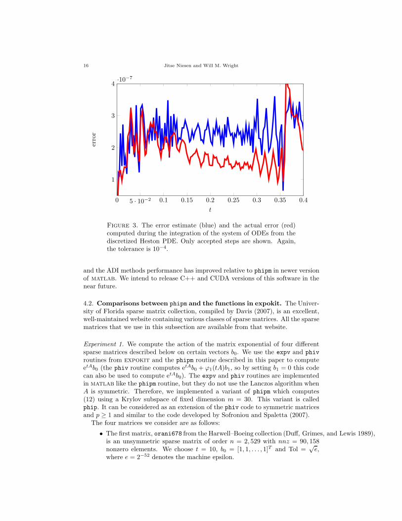
Figure 2 shows how the Krylov subspace size (top graph) and the step size(bottom graph) change during the integration interval. They both vary during theintegration, which shows that the adaptivity presented in Section 3.4 is effective.Figure 3 plots the error estimate and the actual error during the integration interval.The error estimate is always larger than the actual error in this experiment.
One worrying aspect in these figures is that the step size sequence in Figure 2zig-zags and that the estimated error in Figure 3 varies alot from step to step. Thismight indicate stability problems, perhaps caused by augmenting the matrix in (6)or by the matrix-vector multiplications in (16). The matlab solver ode15s alsohas a rather strange stepsize pattern for this problem, where stepsizes are constantor rapidly increasing. The error behaviour of Krylov methods is a difficult problemand we intend to investigate this further in future work; perhaps the use of controltheory techniques can be useful in smoothing the error estimate and choice of Krylovsubspace size. Also, given that this equation has a semi-closed form solution, theapplication to more exotic options, such as barrier, American and Asian options, isof more practical significance and in our minds for future work.
Finally, we draw attention to the fact that the linear algebra in ode15s theCrank–Nicolson and all the ADI methods, is performed using highly optimizedroutines written in a low-level language, whereas all the computations in phipm aredone in the native matlab language. We have noticed that the Crank–Nicolson
16 Jitse Niesen and Will M. Wright
0 5 · 10−2 0.1 0.15 0.2 0.25 0.3 0.35 0.4
1
2
3
4·10−7
t
error
Figure 3. The error estimate (blue) and the actual error (red)computed during the integration of the system of ODEs from thediscretized Heston PDE. Only accepted steps are shown. Again,the tolerance is 10−4.
and the ADI methods performance has improved relative to phipm in newer versionof matlab. We intend to release C++ and CUDA versions of this software in thenear future.
4.2. Comparisons between phipm and the functions in expokit. The Univer-sity of Florida sparse matrix collection, compiled by Davis (2007), is an excellent,well-maintained website containing various classes of sparse matrices. All the sparsematrices that we use in this subsection are available from that website.
Experiment 1. We compute the action of the matrix exponential of four differentsparse matrices described below on certain vectors b0. We use the expv and phiv
routines from expokit and the phipm routine described in this paper to computeetAb0 (the phiv routine computes etAb0 + ϕ1(tA)b1, so by setting b1 = 0 this codecan also be used to compute etAb0). The expv and phiv routines are implementedin matlab like the phipm routine, but they do not use the Lanczos algorithm whenA is symmetric. Therefore, we implemented a variant of phipm which computes(12) using a Krylov subspace of fixed dimension m = 30. This variant is calledphip. It can be considered as an extension of the phiv code to symmetric matricesand p ≥ 1 and similar to the code developed by Sofroniou and Spaletta (2007).
The four matrices we consider are as follows:
• The first matrix, orani678 from the Harwell–Boeing collection (Duff, Grimes, and Lewis 1989),is an unsymmetric sparse matrix of order n = 2, 529 with nnz = 90, 158nonzero elements. We choose t = 10, b0 = [1, 1, . . . , 1]T and Tol =
√e,
where e = 2−52 denotes the machine epsilon.
A Krylov subspace algorithm for evaluating the ϕ-functions 17
• The second example is bcspwr10, also from the Harwell–Boeing collection.This is a symmetric Hermitian sparse matrix of order n = 5, 300 withnnz = 21, 842. We set t = 2, b0 = [1, 0, . . . , 0, 1]T and Tol = 10−5.
• The third example, gr 30 30, again of the Harwell–Boeing collection, is asymmetric matrix arising when discretizing the Laplacian operator using anine-point stencil on a 30 × 30 grid. This yields an order n = 900 sparsematrix with nnz = 7, 744 nonzero elements. Here, we choose t = 2 andcompute e−tAetAb0, where b0 = [1, 1, . . . , 1]T , in two steps: first the forwardstep computes w = etAb0 and then we use the result w as the operandvector for the reverse part e−tAw. The result should approximate b0 withTol = 10−14.
• The final example uses helm2d03 from the GHS indef collection (see (Davis 2007)for more details), which describes the Helmholtz equation−∆T∇u−10000u =1 on a unit square with Dirichlet u = 0 boundary conditions. The result-ing symmetric sparse matrix of order n = 392, 257 has nnz = 2, 741, 935nonzero elements. We compute etAb0 + tϕ1(tA)b1, where t = 2 and b0 =b1 = [1, 1, . . . , 1]T . In this test, only the codes phiv, phip and phipm arecompared, with Tol =
√e.
Only the third example has a known exact solution. To compute the exact solutionsfor the other three examples we use phiv, phipm and expmv from (Al-Mohy and Higham 2010),with a small tolerance so that all methods agree to a suitable level of accuracy. Wereport relative errors computed at the using
error =
∥
∥
∥
∥
uexact − uapprox
uexact
∥
∥
∥
∥
,
where uexact and uapprox are the exact and approximate solutions. When the exactsolution has components which are zero they are removed from the relative errorcalculations. In the first three comparisons we measure the average speedup anderror of each of the codes relative to expv; in the final comparison we measurerelative to phiv. The tic and toc functions from matlab are used to compute thetimings. We ran the comparisons 100 times to compute the average speedup. Wesummarize our findings in Table 1.
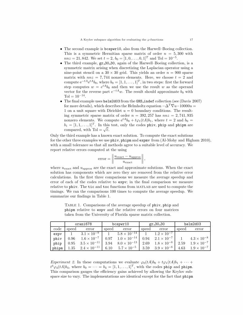
Table 1. Comparisons of the average speedup of phiv, phip andphipm relative to expv and the relative errors on four matricestaken from the University of Florida sparse matrix collection.
orani678 bcspwr10 gr 30 30 helm2d03
code speed error speed error speed error speed errorexpv 1 3.1× 10⁻⁹ 1 5.8× 10⁻¹⁴ 1 1.2× 10⁻⁷
phiv 0.96 1.6× 10⁻⁷ 0.97 1.0× 10⁻¹⁴ 0.94 2.1× 10⁻⁷ 1 4.3× 10⁻⁸
phip 0.95 3.5× 10⁻¹¹ 3.94 8.0× 10⁻¹³ 2.69 1.8× 10⁻⁶ 2.59 1.9× 10⁻⁷
phipm 1.35 2.4× 10⁻¹¹ 6.10 5.7× 10⁻⁵ 3.59 3.9× 10⁻⁶ 4.63 1.9× 10⁻⁷
Experiment 2. In these computations we evaluate ϕ0(tA)b0 + tϕ1(tA)b1 + · · · +t4ϕ4(tA)b4, where b0 = · · · = b4 = [1, 1, . . . , 1]T , with the codes phip and phipm.This comparison gauges the efficiency gains achieved by allowing the Krylov sub-space size to vary. The implementations are identical except for the fact that phipm
18 Jitse Niesen and Will M. Wright
can vary m as well. We use the four sparse matrices described above, with the samevalues of t and Tol, except for the sparse matrix gr 30 30 with Tol =
√e, is used
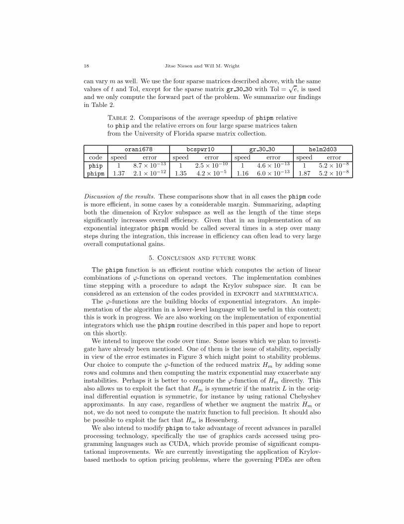
and we only compute the forward part of the problem. We summarize our findingsin Table 2.
Table 2. Comparisons of the average speedup of phipm relativeto phip and the relative errors on four large sparse matrices takenfrom the University of Florida sparse matrix collection.
orani678 bcspwr10 gr 30 30 helm2d03
code speed error speed error speed error speed errorphip 1 8.7× 10⁻¹³ 1 2.5× 10⁻¹⁰ 1 4.6× 10⁻¹³ 1 5.2× 10⁻⁸
phipm 1.37 2.1× 10⁻¹² 1.35 4.2× 10⁻⁵ 1.16 6.0× 10⁻¹³ 1.87 5.2× 10⁻⁸
Discussion of the results. These comparisons show that in all cases the phipm codeis more efficient, in some cases by a considerable margin. Summarizing, adaptingboth the dimension of Krylov subspace as well as the length of the time stepssignificantly increases overall efficiency. Given that in an implementation of anexponential integrator phipm would be called several times in a step over manysteps during the integration, this increase in efficiency can often lead to very largeoverall computational gains.
5. Conclusion and future work
The phipm function is an efficient routine which computes the action of linearcombinations of ϕ-functions on operand vectors. The implementation combinestime stepping with a procedure to adapt the Krylov subspace size. It can beconsidered as an extension of the codes provided in expokit and mathematica.
The ϕ-functions are the building blocks of exponential integrators. An imple-mentation of the algorithm in a lower-level language will be useful in this context;this is work in progress. We are also working on the implementation of exponentialintegrators which use the phipm routine described in this paper and hope to reporton this shortly.
We intend to improve the code over time. Some issues which we plan to investi-gate have already been mentioned. One of them is the issue of stability, especiallyin view of the error estimates in Figure 3 which might point to stability problems.Our choice to compute the ϕ-function of the reduced matrix Hm by adding somerows and columns and then computing the matrix exponential may exacerbate anyinstabilities. Perhaps it is better to compute the ϕ-function of Hm directly. Thisalso allows us to exploit the fact that Hm is symmetric if the matrix L in the orig-inal differential equation is symmetric, for instance by using rational Chebyshevapproximants. In any case, regardless of whether we augment the matrix Hm ornot, we do not need to compute the matrix function to full precision. It should alsobe possible to exploit the fact that Hm is Hessenberg.
We also intend to modify phipm to take advantage of recent advances in parallelprocessing technology, specifically the use of graphics cards accessed using pro-gramming languages such as CUDA, which provide promise of significant compu-tational improvements. We are currently investigating the application of Krylov-based methods to option pricing problems, where the governing PDEs are often
References 19
linear. The corresponding discretized ODEs often take the form of Equation (4),which can naturally be computed using phipm. Finally, as mentioned in the in-troduction, there are alternatives to the (polynomial) Krylov method consideredin this paper. We plan to study other methods and compare them against themethod introduced here. Competitive methods can be added to the code, becausewe expect that the performance of the various methods depends strongly on thecharacteristics of both the problem and the exponential integrator.
Acknowledgements. The authors thank Nick Higham, Karel in ’t Hout, BrynjulfOwren, Roger Sidje and the anonymous referee for helpful discussions.
References
Al-Mohy, A. H. and Higham, N. J. 2010. Computing the action of the matrixexponential, with an application to exponential integrators. Tech. Rep. 30,Manchester Institute for Mathematical Sciences, Manchester, England.
Butcher, J. C. 2008. Numerical methods for ordinary differential equations ,Second ed. John Wiley & Sons Ltd., Chichester.
Caliari, M. and Ostermann, A. 2009. Implementation of exponentialRosenbrock-type integrators. Appl. Numer. Math. 59, 568–581.
Crank, J. and Nicolson, P. 1947. A practical method for numerical evaluationof solutions of partial differential equations of the heat-conduction type. Proc.Cambridge Philos. Soc. 43, 50–67.
Davis, T. A. 2007. The University of Florida sparse matrix collection. Tech.Rep. REP-2007-298, CISE Dept, University of Florida.
Douglas, Jr., J. and Rachford, Jr., H. H. 1956. On the numerical solutionof heat conduction problems in two and three space variables. Trans. Amer.
Math. Soc. 82, 421–439.Duff, I. S., Grimes, R. G., and Lewis, J. G. 1989. Sparse matrix test prob-
lems. ACM Transactions on Mathematical Software 15, 1 (Mar.), 1–14.Friesner, R. A., Tuckerman, L. S., Dornblaser, B. C., and Russo,
T. V. 1989. A method for the exponential propagation of large stiff nonlineardifferential equations. J. Sci. Comput. 4, 4, 327–354.
Gallopoulos, E. and Saad, Y. 1992. Efficient solution of parabolic equationsby Krylov approximation methods. SIAM J. Sci. Statist. Comput. 13, 1236–1264.
Hairer, E.,Nørsett, S. P., andWanner, G. 1993. Solving ordinary differen-
tial equations. I , Second ed. Springer Series in Computational Mathematics,vol. 8. Springer-Verlag, Berlin. Nonstiff problems.
Heston, S. L. 1993. A closed-form solution for options with stochastic volatilitywith applications to bond and currency options. Review of Financial Stud-
ies 6, 2, 327–43.Higham, N. J. 2005. The scaling and squaring method for the matrix exponential
revisited. SIAM J. Matrix Anal. Appl. 26, 4, 1179–1193 (electronic).Higham, N. J. 2008. Functions of matrices. Society for Industrial and Applied
Mathematics (SIAM), Philadelphia, PA. Theory and computation.Hochbruck, M. and Lubich, C. 1997. On Krylov subspace approximations to
the matrix exponential operator. SIAM J. Numer. Anal. 34, 5, 1911–1925.
20 References
Hochbruck, M., Lubich, C., and Selhofer, H. 1998. Exponential integra-tors for large systems of differential equations. SIAM J. Sci. Comput. 19, 5,1552–1574.
Horn, R. A. and Johnson, C. R. 1991. Topics in matrix analysis. CambridgeUniversity Press, Cambridge.
Hundsdorfer, W. and Verwer, J. 2003. Numerical solution of time-
dependent advection-diffusion-reaction equations. Springer Series in Compu-tational Mathematics, vol. 33. Springer-Verlag, Berlin.
In ’t Hout, K. J. 2007. ADI schemes in the numerical solution of the HestonPDE. Numerical Analysis and Applied Mathematics 936, 10–14.
In ’t Hout, K. J. and Foulon, S. 2010. ADI finite difference schemes foroption pricing in the Heston model with correlation. Int. J. Numer. Anal.
Model. 7, 2, 303–320.In ’t Hout, K. J. and Welfert, B. D. 2009. Unconditional stability of
second-order ADI schemes applied to multi-dimensional diffusion equationswith mixed derivative terms. Appl. Numer. Math. 59, 4, 677–692.
Koikari, S. 2007. An error analysis of the modified scaling and squaring method.Computers Math. Applic. 53, 8, 1293–1305.
Koikari, S. 2009. On a block Schur–Parlett algorithm for ϕ-functions based onthe sep-inverse estimate. ACM Trans. on Math. Soft. 38, 2, Article 12.
Lopez-Fernandez, M. 2010. A quadrature based method for evaluatingexponential-type functions for exponential methods. BIT 50, 3, 631–655.
Minchev, B. andWright, W. M. 2005. A review of exponential integrators forsemilinear problems. Tech. Rep. 2/05, Department of Mathematical Sciences,NTNU, Norway. http://www.math.ntnu.no/preprint/.
Moler, C. B. and Van Loan, C. F. 2003. Nineteen dubious ways to computethe exponential of a matrix, twenty-five years later. SIAM Review 45, 1, 3–49.
Moret, I. 2007. On RD-rational Krylov approximations to the core-functionsof exponential integrators. Numer. Linear Algebra Appl. 14, 5, 445–457.
Niesen, J. and Wright, W. M. 2011. Krylov subspace methods applied tooption pricing problems. In preparation.
Saad, Y. 1992. Analysis of some Krylov subspace approximations to the matrixexponential operator. SIAM J. Numer. Anal. 29, 1, 209–228.
Schmelzer, T. and Trefethen, L. N. 2007. Evaluating matrix functions forexponential integrators via Caratheodory–Fejer approximation and contourintegrals. Electronic Transactions on Numerical Analysis 29, 1–18.
Sidje, R. 1998. EXPOKIT: Software package for computing ma-trix exponentials. ACM Trans. on Math. Soft. 24, 1, 130–156. Seehttp://www.maths.uq.edu.au/expokit/ for latest software.
Skaflestad, B. and Wright, W. M. 2009. The scaling and modified squar-ing method for matrix functions related to the exponential. Appl. Numer.
Math. 59, 3-4, 783–799.Sofroniou, M. and Spaletta, G. 2007. Efficient computation of Krylov ap-
proximations to the matrix exponential and related functions. Preprint.Tavella, D. and Randall, C. 2000. Pricing financial instruments. JohnWiley
& Sons Ltd., New York.Trefethen, L. N. and Bau, III, D. 1997. Numerical linear algebra. Society
for Industrial and Applied Mathematics (SIAM), Philadelphia, PA.

References 21
School of Mathematics, University of Leeds, Leeds, LS2 9JT, United Kingdom
E-mail address: [email protected]
Department of Mathematics and Statistics, La Trobe University, 3086 Victoria, Aus-
tralia
E-mail address: [email protected]