A genetic algorithm analysis of resonances in p(γ,K )Λ ...

e

r,

ce in

ymmetrytion

ediateledge

s exist.

Nuclear Physics A 740 (2004) 147–167

www.elsevier.com/locate/np

A genetic algorithm analysis ofN∗ resonancesin p(γ,K+)Λ reactions

D.G. Irelanda,∗, S. Janssenb, J. Ryckebuschb

a Department of Physics and Astronomy, University of Glasgow, Glasgow G12 8QQ, Scotland, UKb Department of Subatomic and Radiation Physics, Ghent University, Proeftuinstraat 86,

B-9000 Gent, Belgium

Received 19 February 2004; received in revised form 5 May 2004; accepted 7 May 2004

Available online 25 May 2004

Abstract

The problem of extracting information on new and knownN∗ resonances by fitting isobamodels to photonuclear data is addressed. A new fitting strategy, incorporating a genetic algorithmis outlined. As an example, the method is applied to a typical tree-level analysis of publishedp(γ,K+)Λ data. It is shown that, within the limitations of this tree-level analysis, a resonanaddition to the known set is required to obtain a reasonable fit. An additionalP11 resonance, with amass of about 1.9 GeV, gives the best agreement with the published data, but additionalS11 or D13resonances cannot be ruled out. Our genetic algorithm method predicts that photon beam asand double polarizationp(γ,K+)Λ measurements should provide the most sensitive informawith respect to missing resonances. 2004 Elsevier B.V. All rights reserved.

PACS:14.20.Gk; 13.60.Le; 02.60.Pn; 02.70.-c

Keywords:Nucleon resonances; Geneticalgorithms; Kaon production

1. Introduction

The spectroscopy of baryons continues to be a subject of great interest in intermenergy nuclear physics, since it an essential component in underpinning our knowof the substructure of the nucleon. Central to this is the issue of which resonance

* Corresponding author.E-mail address:[email protected] (D.G. Ireland).

0375-9474/$ – see front matter 2004 Elsevier B.V. All rights reserved.doi:10.1016/j.nuclphysa.2004.05.007

redict aodels

s.e pionoreposedis the

QCDre ableutental

ory toquark

in thes allng into

an

eachfitting

reesible, aich is

thers and

yinging

iouslyngenessshowducingbaryonecausealysisd, ane need

148 D.G. Ireland et al. / Nuclear Physics A 740 (2004) 147–167

Constituent quark models such as those proposed by Capstick and Roberts [1] plarge number of resonances which thus far have not been observed, whilst for mwhich limit quark degrees of freedom [2], the number of “missing” resonances is les

The majority of resonance information has been gleaned from analyses of singlproduction reactions [3], and the suggestion that the missing resonances may couple mstrongly to other channels [1,4] has led to a number of experiments being proand carried out at intermediate energy accelerator facilities. Of particular interestpossibility of studying strangeness production, since this opensup the possibility ofextracting extraN∗ information.

The use of effective field theories is necessary in the resonance region sincecannot be solved perturbatively at this energy scale. Constituent quark models ato predict quantities such as coupling constants and electromagnetic form factors, bit is not straightforward for these models to predict real observables, as a fundamunderstanding of the underlying dynamics is missing. By using an effective field theextract coupling constants from fits to data, one can obtain numbers to compare withmodel predictions.

A complete understanding of the physics underlying the photonucleon dataresonance region will in principle only be possible in a framework that containparticipating processes which include coupling to resonances [5–9]. This means takiaccount meson production reactions such asγN → πN , ππN , ηN , ωN , KΛ, KΣ, . . . ,

as well as Compton scattering and meson-induced production reactions. This is clearlyenormous task.

In a model adopting effective degrees-of-freedom, the field associated withresonance has a number of free parameters which are usually determined bymodel calculations to data. In a full-blown coupled-channels approach, the number of fparameters could easily end up being over 100. For such a procedure to be possizeable data set for each of the contributing channels is required. One difficulty, whoften overlooked, is the process of how to obtain a set of parameters which leads tobest description of the data. Related to this is the issue of how to assign error baconfidence levels to the values of the extracted resonance parameters.

An analysis of a single channel, whilst not complete, offers the possibility of simplifthe problem by reducing the number of free parameters to a manageable size, and in beable to identify the most important features. Recent attempts to analyse thep(γ,K+)Λ

channel in such a framework have highlighted the tantalising prospect that prevundiscovered resonances may reveal themselves in the mechanisms involving straproduction. Mart and Bennhold [10] used their tree-level hadrodynamical model tothat the total cross-section measured at SAPHIR [11] could be reproduced by introaD13(1895) resonance. This resonance does not appear in the Particle Data Groupsummary table as it had not been conclusively observed, but was included in [10] bof the predicted coupling [1] to strange channels. In addition to this, a recent re-anof pion photoproduction data [12] appeared to find evidence for it. On the other hananalysis by Saghai [13] argued that by tuning the background processes involved, th
for the extra resonance was removed. Both approaches were based on the analysis of theSAPHIR data set, which at that point amounted to around 100 data points.

anceym we

ent ofrole in

thee

ass

orithmntionalhotonn

-levelablescussesisof

esent

ent onlyreested inithmans

ndoundel used

D.G. Ireland et al. / Nuclear Physics A 740 (2004) 147–167 149

In a previous article [14], we highlighted the problem of extracting reliable resoninformation from the limited set ofp(γ,K+)Λ data points by performing manindependent fitting calculations. Using a fitting strategy based on a genetic algorithillustrated that a large number of different solutions resulted in similarχ2 values. Wewere able to group these solutions into two main sets: one withD13 coupling constantsclose to zero (indicating its non-existence), and one with significantly non-zeroD13

coupling constants (indicating its existence). We further showed that the measurempolarization observables, such as photon beam asymmetry, could have a pivotalremoving ambiguities.

We have now performed a systematic study into the feasibility of determiningcombination of resonances which contribute to thep(γ,K+)Λ reaction. To this end, whave used a typical tree-level description of the reaction process in combination withminimization procedure which is specificallydesigned to quantify the relative succeof different combinations of resonances. This procedure employs a genetic algwhich is able to search efficiently a large parameter space, coupled with a conveminimization routine to ensure convergence. We have benefitted from adding new pbeam asymmetry measurements from SPring-8 [15], as well as fitting electroproductiodata measured at Jefferson Lab [16].

The structure of this paper is as follows. We outline the features of a typical treep(γ,K+)Λ reaction model in Section 2. Section 3 describes a framework which enthe extraction of resonance information from existing photonucleon data, and dishow to evaluate the reliability of the information. As an example, the methodologyapplied to a tree-level analysis ofp(γ,K+)Λ in Section 4. We discuss the resultsour work and highlight the important next steps in studying this problem. We prconclusions in Section 5.

2. Model formalism

We adopt a hadrodynamical framework for modelling kaon photoproduction on thnucleon. The model we use has been described in previous work [17], so we presea brief summary here. Thep(γ,K+)Λ reaction process is described by hadronic degof freedom using an effective Lagrangian. The contributioning diagrams are depicFig. 1. Every intermediate particle in the reaction is treated as an effective field wassociated mass, photocoupling amplitudes and strong decay widths. Tree level Feyndiagrams contain the vectorK∗(892) and the axial-vectorK1(1270) t-channel mesons, awell as the usual Born terms. Two hyperon resonances, theS01(1800) andP01(1810) arepresent in theu-channel. These ingredients constitute the so-called “background”.

In Ref. [18] we stressed the difficulties associated with parameterizing the backgroudiagrams inp(γ,K+)Λ calculations and presented results for three plausible backgrschemes. Subsequent work [19] showed that thep(e, e′K+)Λ process is highly selectivwith respect to viable choices for dealing with the background diagrams. The mode
here is the only one which we found to reproduce simultaneously thep(γ,K+)Λ andp(e, e′K+)Λ data.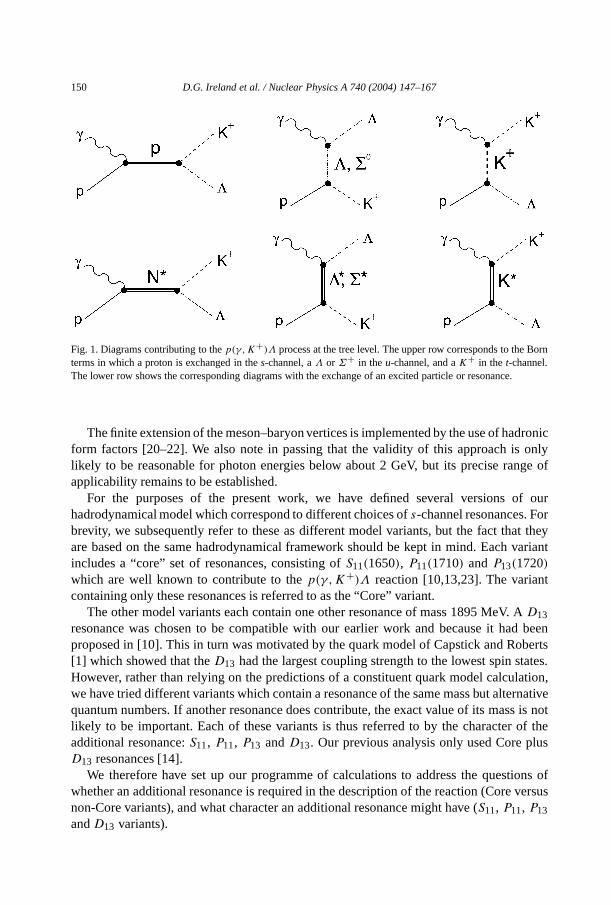

Born

droniconly

nge of

of ourort theyvariant

t

d beenbertstes.

lation,rnativeothelus

ions ofversus


Fig. 1. Diagrams contributing to thep(γ,K+)Λ process at the tree level. The upper row corresponds to theterms in which a proton is exchanged in thes-channel, aΛ or Σ+ in theu-channel, and aK+ in the t-channel.The lower row shows the corresponding diagrams withthe exchange of an excited particle or resonance.

The finite extension of the meson–baryon vertices is implemented by the use of haform factors [20–22]. We also note in passing that the validity of this approach islikely to be reasonable for photon energies below about 2 GeV, but its precise raapplicability remains to be established.

For the purposes of the present work, we have defined several versionshadrodynamical model which correspond to different choices ofs-channel resonances. Fbrevity, we subsequently refer to these as different model variants, but the fact thaare based on the same hadrodynamical framework should be kept in mind. Eachincludes a “core” set of resonances, consisting ofS11(1650), P11(1710) andP13(1720)which are well known to contribute to thep(γ,K+)Λ reaction [10,13,23]. The variancontaining only these resonances is referred to as the “Core” variant.

The other model variants each containone other resonance of mass 1895 MeV. AD13

resonance was chosen to be compatible with our earlier work and because it haproposed in [10]. This in turn was motivated by the quark model of Capstick and Ro[1] which showed that theD13 had the largest coupling strength to the lowest spin staHowever, rather than relying on the predictions of a constituent quark model calcuwe have tried different variants which contain a resonance of the same mass but altequantum numbers. If another resonance does contribute, the exact value of its mass is nlikely to be important. Each of these variants is thus referred to by the character of tadditional resonance:S11, P11, P13 andD13. Our previous analysis only used Core pD13 resonances [14].

We therefore have set up our programme of calculations to address the questwhether an additional resonance is required in the description of the reaction (Core
non-Core variants), and what characteran additional resonance might have (S11, P11, P13
andD13 variants).

s.rentialt [11],d

16], as].s

f theirngin

ofor

irefor eachcedure

d thebeing

bars onh these

arers (asrue ifg thel data,

ave’s


3. Analysis procedure

For each model variant, we performed a set of calculations to extractN∗ informationfrom the reaction data. Each set consisted of100 separate minimization calculationThe data sets employed in the fitting procedure included total cross-sections, diffephoto-production cross-sections and recoil polarizations from the SAPHIR data seand photon beam-polarization asymmetriesfrom SPring-8 [15]. In addition, we also useseparated longitudinal and transverse electroproduction data from Jefferson Lab [well as total electroproduction cross sections from a variety of older sources [24–26

The coupling constants associated with the hadronic vertices in all the amplitudeincluded in the model are free parameters in the fitting procedure. A description oexact definition is given in [27], but we brieflylist them here for completeness: coupliconstants related to Born terms,gK+Λp andgK+Σp ; vector and axial vector mesonsthe t-channel,Gv

K∗ , GtK∗ , Gv

K1andGt

K1; spin-12 Y ∗ resonances in theu-channel,GY ∗Kp ;

spin-12 N∗ resonances in thes-channel,GN∗KΛ; spin-32 N∗ resonances in thes-channel,G1

N∗KΛ, G2N∗KΛ and three off-shell parameters. Note that these constants are products

both a hadronic part and an electromagnetic part. Two hadronic cut-off parameters (one fall the Born terms,Λborn, and for all resonances in thes-, t- andu-channels,Λres) are alsofree parameters.

To compare the relative success of each model variant in describing the data, we requtwo separate but related procedures: a search for the best set of free parametersmodel variant, and a comparison amongst the different model variants. The first prois achieved by varying the free parameters and searching for a minimumχ2 statistic byfitting calculations to the data. This is a fairly standard procedure, but we reminreader in passing the assumptions which are implicitly required: the data pointsfitted must be independent (the value of one does not affect the others), and errorthe points represent the standard deviations of a Gaussian probability density. Botrequirements are likely to be approximately correct, and thus minimisingχ2 is equivalentto maximising a likelihood function. The likelihood represents the probability that the datawould be measured, given a particular set of free parameters.

Furthermore, there is the assumption that no particular values of the free parametersto be favoured prior to the fitting procedure. By imposing limits on the free parametewe do through physics constraints) this is not strictly true, but will be approximately tthe limits are sufficiently large. The whole procedure is then equivalent to maximisinprobability that a particular set of free parameters is correct, given the experimentaby varying the free parameters.

Comparing different model variants needs to be done carefully, since each one may ha different number of free parameters. The approach we take implicitly employs “Occamrazor” by penalising model variants with more free parameters.

3.1. Fitting

Each model variant has at least 20 parameters which need to be extracted by fitting thecalculations to the data. Traditional optimizing routines require a first guess at parameter

ad bywas

A) inA

sonableowelltima,ys to

puting.the

domly.rs

thee the

bles

Onereaternare

f thebyories.

andd:

in theapointsone

hownationst-


values. Whilst some prior experience can beused to estimate the starting values, inparameter space of this size it is very difficult to judge whether an optimum founan optimizer is local or global. In previous work [17] a simulated annealing strategyadopted, however we subsequently found [14] that using a genetic algorithm (Gcombination with a traditional optimizer, MINUIT [28], offered many advantages. The Gis able to search a large region of parameter space and very quickly arrives at reasolutions, whereas a minimizer such as MINUIT, which uses a Davidon–Fletcher–Palgorithm, is able to take the solutions from the GA as starting points and find opprovided the starting points are not too far from the optimum. This strategy thus plathe strengths of both algorithms.

Genetic algorithms are a class of search strategies known as evolutionary comA number of excellent texts on GAs exist (e.g., [29,30]), so we will only briefly sketchstrategy we have employed. The idea is to generate a number of trial solutions ranIn this implementation, each solution is an encoding of trial values of the free parameteas a string of real numbers{λi}, whereλi represents the value of free parameteri.

The collection of solutions is referred to as a “population”. Each solution inpopulation is used to evaluate a function which determines its “fitness”. In our casfitness function is

f {λi} = 1

1+ χ2{λi} ,

whereχ2{λi} is the result of running the calculation of all the experimental observaand comparing with the available data.

The population is then “evolved” in a manner analogous to biological evolution.or two solutions are selected from the current population, where solutions with gfitness function values are selected preferentially, but not exclusively. When one solutiois selected, it is subjected to a “mutation”, where one or more of the free parametersaltered at random.

When two solutions are selected, a new individual is created by “crossover” oencoded parameters in each solution. In thisimplementation, crossover is performeda number of different functions, chosen at random, which fall broadly into two categThe first is to swap one or more parameters from solution{λi} to solution{µi}, λi ↔ µi

two obtain two “child” solutions. The second takes parameters from each solutionforms one child by assigning it new parameters{νi} calculated by a weighted averageνi = w1λi+w2µi

w1+w2.

A new fitness is then evaluated, and if it is better than the worst current fitnesspopulation, the new solution replaces the previous worst. This is often referred to assteady state GA. The population therefore gradually migrates to one or more betterin parameter space, and if the routine is run for long enough, it will converge onoptimum. Whilst this optimum is not guaranteed to be global, GA research [30] has sthat “reasonable” solutions can be found very efficiently, even when no prior informhas been used to constrain the free parameters.For instance, in our calculations, the beof-generation solutions at the start of a run haveχ2 values of order 106 but this will be
reduced to of order 10 after only 5000 evaluations of the objective function. If gradientmethods were employed using such a random choice of initial starting values, it is highly

latedber offor allwith

end

00er

aintidual

n

ngeduced

g the

UITheed

inceouldre,neficial

. At

nted a

re

tat thezation


likely they would be trapped in local minima. Note also that compared to the simuannealing strategy used in previous work [17–19,31] we have reduced the numfunction evaluations by a factor of 10. Whereas no one strategy can be optimumproblems, the GA is likely to be highly efficient for problems such as the present onemany parameters and complicatedχ2 surfaces. The best-of-generation solutions at theof each GA run can be used as starting points for a MINUIT minimization.

The complete strategy for analysis of each model was as follows:

(1) 100 GA calculations were initiated. Each GA calculation used a population of 2and was run for 5000 evaluations of the objective function. The limits for each parametwere deliberately chosen to define a large region of parameter space;

(2) The best solution from each GA calculation was used as a starting point forMINUIT minimization which was run for a further 5000 function evaluations. At this povery few, if any, of the MINUIT calculations had achieved convergence and the resvalues ofχ2 were too high; a more limited search space was required;

(3) The parameters associated with eachof the 100 MINUIT solutions were theexamined. The set of solutions whoseχ2 values were within 1.0 of the current bestχ2

were selected. A new, tighter set of limitsfor each parameter was defined from the raof parameter values exhibited by the chosen subset of solutions. This typically reparameter ranges by factors of 5–10;

(4) 100 new GA calculations were initiated, the only difference from before beinsmaller region of parameter space inwhich the search was performed;

(5) As before, the best solution from each GA calculation was used to initiate MINcalculations. A few calculations had convergedat this point. It was clear, however, that tcalculations had not converged to the same optimum, so to investigate this, we proceedto try to obtain convergence for all the calculations;

(6) The MINUIT solutions were then re-inserted back into the GA populations. Sthe inserted solution was likely to be the “fittest” solution in the population, this wcause the GA to concentrate more on a particular region of parameter space. Furthermothe populations from each of the 100 GA calculations were mixed. This is a variation owhat is known as an island population mixing scheme, and can be shown to be benin cases where separate GAs are converging on different optima;

(7) A third run of the 100 GA calculations was now performed;(8) A final MINUIT calculation for each of the 100 GA best solutions was done

this point, all the calculations had converged.

The result for each model variant was 100 solutions, each of which represeconverged minimization by MINUIT. As we noted in [14], we observed thateach solutionwas unique,even although they had roughly similarχ2 values. In other words, there weat least100 local minima in theχ2 surface.

The fact that each calculation appears to finda different local minimum shows thathe optimization problem may be ill-posed. The reason for this could be either threaction model lacks an ingredient which is necessary to obtain reproducible minimi
results, or that the experimental data contain systematic uncertainties which render theminconsistent with each other, or that both themodel and the data are problematic. From

uplingbydata

h theusns ofingsed in] and

duction). This(e.g.,e the

regionork we

he

gionedllyismodel,f either

r

mle

camily


this observation, we caution that it is not possible to extract the magnitudes of coconstants to high precision by fitting hadrodynamical models such as ours (andextension other similar models) to a relatively small number of photoproductionpoints.

What is observed however, is that the “best” of the calculations (i.e., those witlowestχ2 values) tend to cluster around particularregions in parameter space. Our previowork [14] showed that this still resulted in considerable ambiguities in the calculatioun-measured observables, and pointed to quantities such as photon asymmetry as bevery useful in reducing the uncertainties in parameter values. The additional data uthe present work are the beam polarization data from the SPring-8/LEPS facility [15electroproduction data [16,24–26], and it appears they have affected a marked rein the regions of parameter space which give a good fit to the data (see Section 4is a valuable observation. It shows that our original work, in agreement with others[10]), was able to predict the measurements which would most significantly improvcomparison between data and theory.

3.2. Model variant comparison

Whilst the best fit for each model was obtained by minimisingχ2, this does not takeinto account the different number of free parameters in each model, or how small aof parameter space corresponds to a reasonable fit. A full description of the framewhave employed is given in the appendix, but we sketch the salient points here.

Comparing two model variants (A and B, say), we can evaluate the ratio of tlikelihood functions:

P(D|A)

P(D|B), (1)

whereP(D|A) (P(D|B)) is the probability that the dataD would be obtained, assuminthat variant A (B) were true. Under some reasonable assumptions (as mentpreviously), minimisingχ2 is equivalent to maximising the likelihood, but what is actuaobtained could be written asP(D|λMP

i ,A) (where MP stands for “most probable”). Thexpression indicates that the maximum likelihood depends on the parameters of theλi , whereas Eq. (1) requires there to be no dependence on the free parameters ovariant.

Using further approximations, we obtain for variantA the expression (with a similaone for variantB):

P(D|A) ∝ P(D

∣∣λMP,A) ∏N

i δλMPi∏N

i (λmaxi − λmin

i ), (2)

where there areN free parameters,λmaxi andλmin

i represent the maximum and minimulimits of search space for parameterλi , andδλMP

i is the uncertainty in the most probabvalue of parameterλi . The second factor in Eq. (2) is often referred to as the “Ocfactor”, since it penalizes model variants with more free parameters. It is most eas
interpreted as a product ofN factors, each one a ratio of fitted error bar size to searchspace size for parameterλi . Model variants whose parameter error bars are relatively large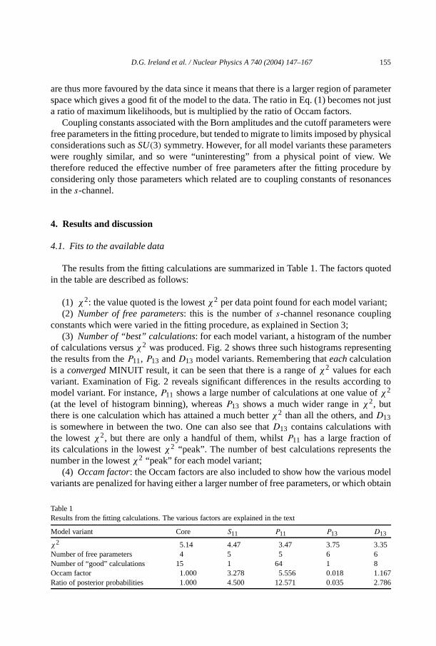

terot just

rs werealtersWe

ure bynances

ted

t;g

bernting

of

fe

eltain


are thus more favoured by the data since it means that there is a larger region of paramespace which gives a good fit of the model to the data. The ratio in Eq. (1) becomes na ratio of maximum likelihoods, but is multiplied by the ratio of Occam factors.

Coupling constants associated with the Born amplitudes and the cutoff parametefree parameters in the fitting procedure, but tended to migrate to limits imposed by physicconsiderations such asSU(3) symmetry. However, for all model variants these paramewere roughly similar, and so were “uninteresting” from a physical point of view.therefore reduced the effective number of free parameters after the fitting procedconsidering only those parameters which related are to coupling constants of resoin thes-channel.

4. Results and discussion

4.1. Fits to the available data

The results from the fitting calculations are summarized in Table 1. The factors quoin the table are described as follows:

(1) χ2: the value quoted is the lowestχ2 per data point found for each model varian(2) Number of free parameters: this is the number ofs-channel resonance couplin

constants which were varied in the fitting procedure, as explained in Section 3;(3) Number of “best” calculations: for each model variant, a histogram of the num

of calculations versusχ2 was produced. Fig. 2 shows three such histograms represethe results from theP11, P13 andD13 model variants. Remembering thateachcalculationis a convergedMINUIT result, it can be seen that there is a range ofχ2 values for eachvariant. Examination of Fig. 2 reveals significant differences in the results according tmodel variant. For instance,P11 shows a large number of calculations at one value oχ2

(at the level of histogram binning), whereasP13 shows a much wider range inχ2, butthere is one calculation which has attained a much betterχ2 than all the others, andD13is somewhere in between the two. One can also see thatD13 contains calculations withthe lowestχ2, but there are only a handful of them, whilstP11 has a large fraction oits calculations in the lowestχ2 “peak”. The number of best calculations represents thnumber in the lowestχ2 “peak” for each model variant;

(4) Occam factor: the Occam factors are also included to show how the various modvariants are penalized for having either a larger number of free parameters, or which ob

Table 1Results from the fitting calculations. The various factors are explained in the text

Model variant Core S11 P11 P13 D13

χ2 5.14 4.47 3.47 3.75 3.35Number of free parameters 4 5 5 6 6Number of “good” calculations 15 1 64 1 8Occam factor 1.000 3.278 5.556 0.018 1.167
Ratio of posterior probabilities 1.000 4.500 12.571 0.035 2.786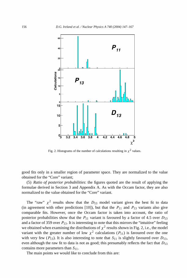

value

theo

ta

tio of

gele

at


Fig. 2. Histograms of the number of calculations resulting inχ2 values.

good fits only in a smaller region of parameter space. They are normalized to theobtained for the “Core” variant;

(5) Ratio of posterior probabilities: the figures quoted are the result of applyingformulae derived in Section 3 and Appendix A. As with the Occam factor, they are alsnormalized to the value obtained for the “Core” variant.

The “raw” χ2 results show that theD13 model variant gives the best fit to da(in agreement with other predictions [10]), but that theP11 and P13 variants also givecomparable fits. However, once the Occam factor is taken into account, the raposterior probabilities show that theP11 variant is favoured by a factor of 4.5 overD13

and a factor of 359 overP13. It is interesting to note that this mirrors the “intuitive” feelinwe obtained when examining the distributions ofχ2 results shown in Fig. 2, i.e., the modvariant with the greater number of lowχ2 calculations (P11) is favoured over the onwith very few (P13). It is also interesting to note thatS11 is slightly favoured overD13,even although the raw fit to data is not as good; this presumably reflects the fact thD13

contains more parameters thanS11.The main points we would like to conclude from this are:

ant

al

certainsupport

ectionng14]reatw dataionduced.cegst the

ilhichl cross-

edtotal


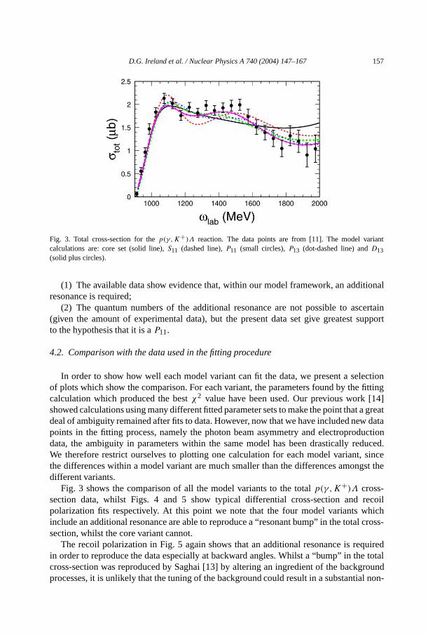
Fig. 3. Total cross-section for thep(γ,K+)Λ reaction. The data points are from [11]. The model varicalculations are: core set (solid line),S11 (dashed line),P11 (small circles),P13 (dot-dashed line) andD13(solid plus circles).

(1) The available data show evidence that,within our model framework, an additionresonance is required;

(2) The quantum numbers of the additional resonance are not possible to as(given the amount of experimental data), but the present data set give greatestto the hypothesis that it is aP11.

4.2. Comparison with the data used in the fitting procedure

In order to show how well each model variant can fit the data, we present a selof plots which show the comparison. For eachvariant, the parameters found by the fitticalculation which produced the bestχ2 value have been used. Our previous work [showed calculations using many different fitted parameter sets to make the point that a gdeal of ambiguity remained after fits to data. However, now that we have included nepoints in the fitting process, namely the photon beam asymmetry and electroproductdata, the ambiguity in parameters within the same model has been drastically reWe therefore restrict ourselves to plotting one calculation for each model variant, sinthe differences within a model variant are much smaller than the differences amondifferent variants.

Fig. 3 shows the comparison of all the model variants to the totalp(γ,K+)Λ cross-section data, whilst Figs. 4 and 5 show typical differential cross-section and recopolarization fits respectively. At this point we note that the four model variants winclude an additional resonance are able to reproduce a “resonant bump” in the totasection, whilst the core variant cannot.

The recoil polarization in Fig. 5 again showsthat an additional resonance is requirin order to reproduce the data especially at backward angles. Whilst a “bump” in the
cross-section was reproduced by Saghai [13] by altering an ingredient of the backgroundprocesses, it is unlikely that the tuning of the background could result in a substantial non-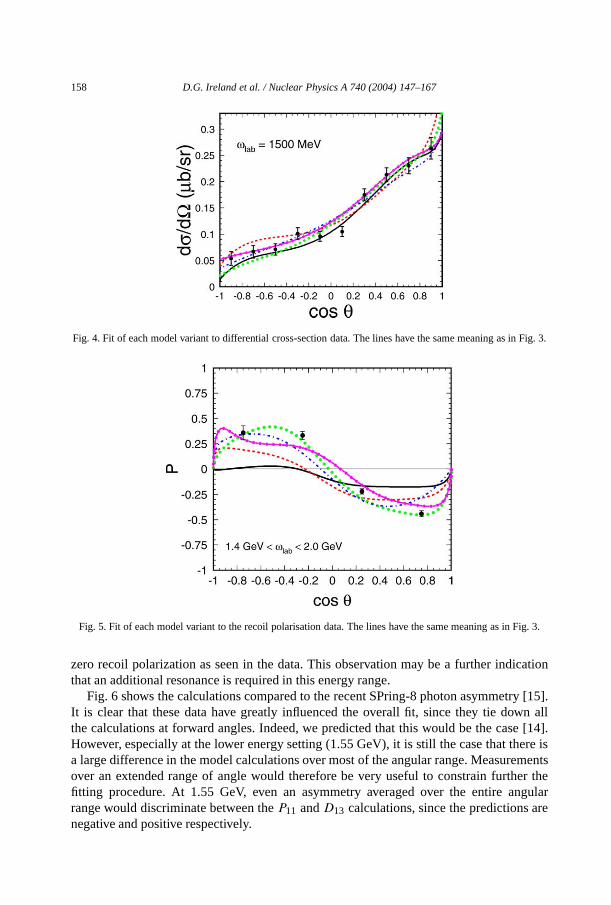

Fig. 3.

3.

n

5].wn all4].ere ismentse

ngular


Fig. 4. Fit of each model variant to differential cross-section data. The lines have the same meaning as in

Fig. 5. Fit of each model variant to the recoil polarisation data. The lines have the same meaning as in Fig.

zero recoil polarization as seen in the data. This observation may be a further indicatiothat an additional resonance is required in this energy range.

Fig. 6 shows the calculations compared tothe recent SPring-8 photon asymmetry [1It is clear that these data have greatly influenced the overall fit, since they tie dothe calculations at forward angles. Indeed, we predicted that this would be the case [1However, especially at the lower energy setting (1.55 GeV), it is still the case that tha large difference in the model calculations over most of the angular range. Measureover an extended range of angle would therefore be very useful to constrain further thfitting procedure. At 1.55 GeV, even an asymmetry averaged over the entire a
range would discriminate between theP11 andD13 calculations, since the predictions arenegative and positive respectively.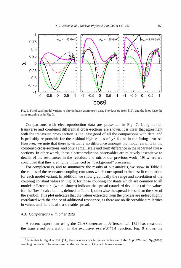

the

dinal,entta, and.in thess-itive tore we

2ulationof theto allalues

size ofhighly

ilarities

surede


Fig. 6. Fit of each model variant to photon beam asymmetry data. The data are from [15], and the lines havesame meaning as in Fig. 3.

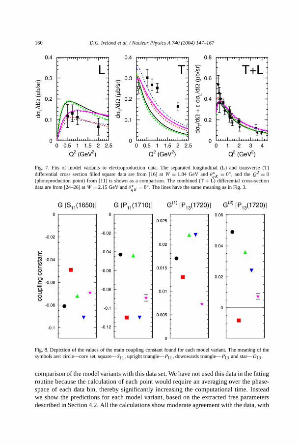
Comparisons with electroproduction data are presented in Fig. 7. Longitutransverse and combined differential cross-sections are shown. It is clear that agreemwith the transverse cross section is the least good of all the comparisons with dais probably responsible for the residual high values ofχ2 found in the fitting processHowever, we note that there is virtually no difference amongst the model variantscombined cross-sections, and only a small scale and form difference in the separated crosections. In other words, these electroproduction observables are relatively insensdetails of the resonances in the reaction, and mirror our previous work [19] wheconcluded that they are highly influenced by “background” processes.

For completeness, and to summarize the results of our analysis, we show in Tablethe values of the resonance coupling constants which correspond to the best fit calcfor each model variant. In addition, we show graphically the range and correlationcoupling constant values in Fig. 8, for those coupling constants which are commonmodels.1 Error bars (where shown) indicate the spread (standard deviation) of the vfor the “best” calculations, defined in Table 1, otherwise the spread is less than thethe symbol. This plot indicates that the values extracted from the process are indeedcorrelated with the choice of additional resonance, as there are no discernable simin values and there is also a sizeable spread.

4.3. Comparisons with other data

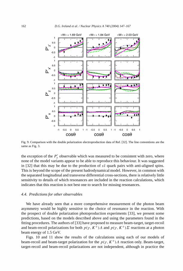
A recent experiment using the CLAS detector at Jefferson Lab [32] has meathe transferred polarization in the exclusivep(�e, e′K+) �Λ reaction. Fig. 9 shows th

1 Note that in Fig. 4 of Ref. [14], there was an error in the normalisation of theP13(1720) andD13(1895)coupling constants. The values used in thecalculations of that article were correct.

(T)

of the

fittingase-ad


Fig. 7. Fits of model variants to electroproduction data. The separated longitudinal (L) and transversedifferential cross section filled square data are from [16] atW = 1.84 GeV andθ�

qK= 0◦, and theQ2 = 0

(photoproduction point) from [11] is shown as a comparison. The combined (T+ L) differential cross-sectiondata are from [24–26] atW = 2.15 GeV andθ�

qK= 8◦ . The lines have the same meaning as in Fig. 3.

Fig. 8. Depiction of the values of the main coupling constant found for each model variant. The meaningsymbols are: circle—core set, square—S11, upright triangle—P11, downwards triangle—P13 and star—D13.

comparison of the model variants with this data set. We have not used this data in theroutine because the calculation of each point would require an averaging over the phspace of each data bin, thereby significantly increasing the computational time. Inste
we show the predictions for each model variant, based on the extracted free parametersdescribed in Section 4.2. All the calculations show moderate agreement with the data, with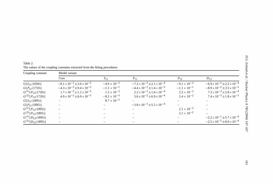

D.G

.Irela

nd

eta

l./Nucle

ar

Physics

A740

(2004)

147–167

161

P13 D13

−9.1× 10−2 −6.9×10−2 ±2.2×10−4

−1.1× 10−1 −8.9×10−2 ±3.5×10−3

2.2× 10−2 7.3×10−3 ±2.8×10−4

2.4× 10−2 7.4×10−3 ±1.8×10−3

– –– –

2.1× 10−2 –2.1× 10−2 –

– −2.2×10−1 ±5.7×10−4

– −2.5×10−2 ±8.0×10−4

Table 2The values of the coupling constants extracted from the fitting procedures

Coupling constant Model variant

Core S11 P11

G[S11(1650)] −8.1×10−2±3.6×10−5 −4.9× 10−2 −7.2×10−2±2.1×10−4

G[P11(1710)] −4.3×10−2±9.4×10−5 −1.1× 10−1 −4.4×10−2±1.4×10−3

G(1)[P13(1720)] 1.7×10−2±1.2×10−5 1.3× 10−2 2.2×10−2±1.6×10−4

G(2)[P13(1720)] 4.9×10−2±6.0×10−5 −8.2× 10−3 3.6×10−2±6.9×10−4

G[S11(1895)] – 8.7× 10−2 –G[P11(1895)] – – −3.8×10−1±5.5×10−4

G(1)[P13(1895)] – – –G(2)[P13(1895)] – – –G(1)[D13(1895)] – – –G(2)[D13(1895)] – – –

the

heregested

s.n withly littlewhich

n beamWithsomed in thecoiln

els of


Fig. 9. Comparison with the double polarization electroproduction data of Ref. [32]. The line conventions aresame as Fig. 3.

the exception of theP ′x observable which was measured to be consistent with zero, w

none of the model variants appear to be able to reproduce this behaviour. It was sugin [32] that this may be due to the production ofss̄ quark pairs with anti-aligned spinThis is beyond the scope of the present hadrodynamical model. However, in commothe separated longitudinal and transverse differential cross-sections, there is relativesensitivity to details of which resonances are included in the reaction calculations,indicates that this reaction is not best one to search for missing resonances.

4.4. Predictions for other observables

We have already seen that a more comprehensive measurement of the photoasymmetry would be highly sensitive to the choice of resonance in the reaction.the prospect of double polarization photoproduction experiments [33], we presentpredictions, based on the models described above and using the parameters founfitting procedures. The authors of [33] have proposed to measure beam-target, target-reand beam-recoil polarizations for bothp(γ,K+)Λ andp(γ,K+)Σ reactions at a photobeam energy of 1.5 GeV.

Figs. 10 and 11 show the results of the calculations using each of our mod
beam-recoil and beam-target polarization for thep(γ,K+)Λ reaction only. Beam-target,target-recoil and beam-recoil polarizations are not independent, although in practice the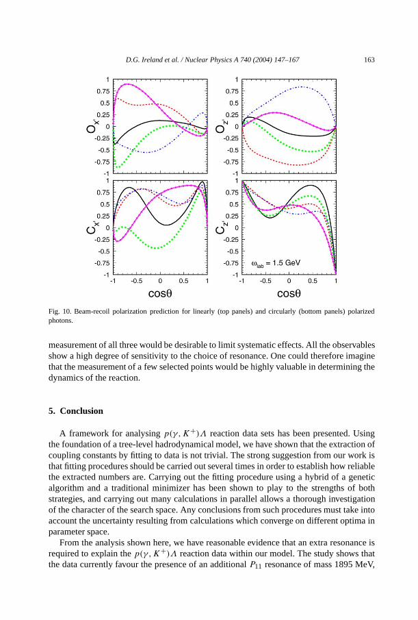

ed

lesaginee

singtion ofrk isleticboth

gationntoin

e is


Fig. 10. Beam-recoil polarization prediction for linearly(top panels) and circularly (bottom panels) polarizphotons.

measurement of all three would be desirable to limit systematic effects. All the observabshow a high degree of sensitivity to the choice of resonance. One could therefore imthat the measurement of a few selected points would be highly valuable in determining thdynamics of the reaction.

5. Conclusion

A framework for analysingp(γ,K+)Λ reaction data sets has been presented. Uthe foundation of a tree-level hadrodynamical model, we have shown that the extraccoupling constants by fitting to data is not trivial. The strong suggestion from our wothat fitting procedures should be carried out several times in order to establish how reliabthe extracted numbers are. Carrying out the fitting procedure using a hybrid of a genealgorithm and a traditional minimizer has been shown to play to the strengths ofstrategies, and carrying out many calculations in parallel allows a thorough investiof the character of the search space. Any conclusions from such procedures must take iaccount the uncertainty resulting from calculations which converge on different optimaparameter space.

From the analysis shown here, we have reasonable evidence that an extra resonanc
required to explain thep(γ,K+)Λ reaction data within our model. The study shows thatthe data currently favour the presence of an additionalP11 resonance of mass 1895 MeV,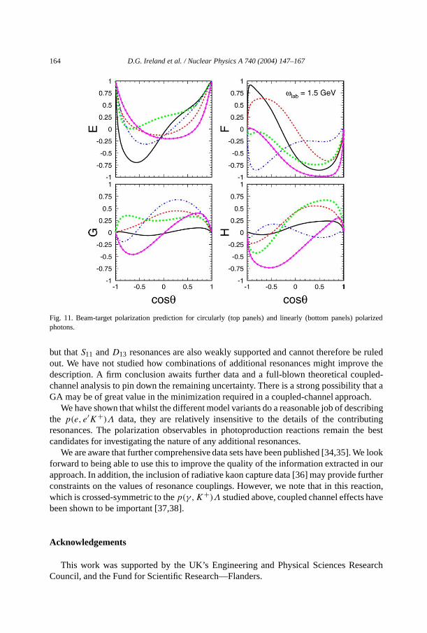

d

ruledve thed-that a

ch.ribingtingest

e lookn oururtheraction,ave


Fig. 11. Beam-target polarization prediction for circularly (top panels) and linearly (bottom panels) polarizephotons.

but thatS11 andD13 resonances are also weakly supported and cannot therefore beout. We have not studied how combinations of additional resonances might improdescription. A firm conclusion awaits further data and a full-blown theoretical couplechannel analysis to pin down the remaining uncertainty. There is a strong possibilityGA may be of great value in the minimization required in a coupled-channel approa

We have shown that whilst the different model variants do a reasonable job of descthe p(e, e′K+)Λ data, they are relatively insensitive to the details of the contriburesonances. The polarization observables in photoproduction reactions remain the bcandidates for investigating the nature of any additional resonances.

We are aware that further comprehensive data sets have been published [34,35]. Wforward to being able to use this to improve the quality of the information extracted iapproach. In addition, the inclusion of radiative kaon capture data [36] may provide fconstraints on the values of resonance couplings. However, we note that in this rewhich is crossed-symmetric to thep(γ,K+)Λ studied above, coupled channel effects hbeen shown to be important [37,38].

Acknowledgements

This work was supported by the UK’s Engineering and Physical Sciences ResearchCouncil, and the Fund for Scientific Research—Flanders.

os

haves the

hate

itswere

orsate

trix


Appendix A. Model comparison

We compare the relative success of the different model variants by evaluating the ratiof the maximum posterior probabilities [39]. To compare variantsA andB the ratio, afterapplication of BayesTheorem, becomes

P(A|D)

P(B|D)= P(D|A)P(A)

P(D|B)P(B),

where P(A|D) is the maximum posterior probability for variantA, P(D|A) is theprobability that the data would be obtained, assuming variantA to be true,P(A) is thea priori probability that variantA is correct and similarly for variantB. With no priorprejudice as to which variant is correct, we obtain the ratio of likelihoods:

P(D|A)

P(D|B).

The likelihoodP(D|A) is an integral over the joint likelihoodP(D, {λi }|A), where{λi}represents a set of free parameters:

P(D|A) =∫

P(D,λi |A)dλi

=∫

P(D|λi ,A)P (λi |A)dλi, (A.1)

where we have dropped the curly brackets for convenience. Model variants maydifferent numbers of parameters, and the multi-dimensional integral in Eq. (A.1) iformal means of handling the problem. The functionP(λi |A) is the prior probabilitythat the parameters take on specific values. With no prior prejudice, we assume teach parameterλi lies in the rangeλmin

i � λi � λmaxi , and we can write the prior as th

reciprocal of the volume of a hypercube in parameter search space (N -dimensional forNfree parameters):

P(λi |A) = 1∏Ni (λmax

i − λmini )

.

To evaluate the volume of the hypercube in parameter space for each variant, the limdefined after the first GA plus MINUIT calculations were used, and in general theydifferent for each variant.

The factorP(D|λi ,A) in the integrand of Eq. (A.1) is not trivial to evaluate. If the errin the fitted parameters,δλMP

i corresponding to the maximum likelihood are multivariGaussian, it can be shown that

P(D|λi ,A) ∝ P(D

∣∣λMPi ,A

)Det−

12

(H2π

), (A.2)

whereH = − �2 lnP(λ|D,A) is the Hessian matrix, and is the inverse of the error ma
obtained in the fitting process which yieldsλMP. The explanations for this are given instandard texts on Bayesian data analysis [39].

case.sentingded totheeters,he

s and

s fromt of

willeing


Eq. (A.2) can thus be written as

P(D|A) ∝ P(D

∣∣λMPi ,A

) Det− 12 ( H

2π)∏N

i (λmaxi − λmin

i ), (A.3)

where the second factor is the Occam factor. We make a further simplification in ourAs mentioned in the main text, some of the free parameters, such as those reprecoupling constants associated with Born amplitudes and cutoff parameters tenmigrate to limits. Apart from being physically “uninteresting”, this also causeddeterminant of the error matrix to be very sensitive to details of these fitted paramsince the errors on each were very small. Thephysically interesting parameters are tones which relate to resonances in thes-channel.

Rather than redoing the whole minimization procedure with fixed Born amplitudecutoffs (which we deemed unnecessary due to the likely inaccuracy of the results fromfitting to a limited data set), we took the errors on the most probable parameter valuethe MINUIT calculations. MINUIT returns values which take into account the effeccorrelations amongst parameters, so we applied the approximation

Det−12

(H2π

)=

M∏i

δλMPi ,

whereM is the reduced number of parameters.The Occam factor for each variant was therefore reduced to∏M

i δλMPi∏M

i (λmaxi − λmin

i ).

The first factor in Eq. (A.3) can be evaluated up to a scale factor by

P(D

∣∣λMP,A) ∝ exp

(−χ2

2

).

Hence, by taking a ratio of the total likelihoods for two variants, all common factorsdivide out, leaving a figure which represents the relative probability of two variants bcorrect.

References

[1] S. Capstick, W. Roberts, Phys. Rev. D 58 (1998) 074011.[2] M. Oettel, R. Alkofer, L. von Smekal, Eur. Phys. J. A 8 (2000) 553.[3] Particle Data Group, D.E. Groom, et al., Eur. Phys. J. C 15 (2000) 1.[4] S. Capstick, W. Roberts, Phys. Rev. D 49 (1994) 4570.[5] D. Manley, E. Saleski, Phys. Ref. D 45 (1992) 4002.[6] T. Vrana, S. Dytman, T.-S. Lee, Phys. Rep. 328 (1999) 181.[7] G. Penner, U. Mosel, Phys. Rev. C 66 (2002) 055212.[8] W.-T. Chiang, F. Tabakin, T.-S. Lee, B. Saghai, Phys. Lett. B 517 (2001) 101.
[9] N. Kaiser, T. Waas, W. Weise, Nucl. Phys. A 612 (1997) 297.
[10] T. Mart, C. Bennhold, Phys. Rev. C 61 (2000) (R)012201.

Physics

1) 105.

y,


[11] M.Q. Tran, et al., Phys. Lett. B 445 (1998) 20.[12] R. Crawford, in: S. Dytman, S. Swanson (Eds.), Proceedings of the NSTAR 2002 Workshop on the

of Excited Nucleons, World Scientific, New Jersey, 2002, p. 256.[13] B. Saghai, nucl-th/0105001.[14] S. Janssen, D. Ireland, J. Ryckebusch, Phys. Lett. B 562 (2003) 51.[15] R.G.T. Zegers, et al., Phys. Rev. Lett. 91 (9) (2003) 092001.[16] R.M. Mohring, et al., Phys. Rev. C 67 (2003) 055205.[17] S. Janssen, J. Ryckebusch, W. Van Nespen, D. Debruyne, T. Van Cauteren, Eur. Phys. J. A 11 (200[18] S. Janssen, J. Ryckebusch, D. Debruyne, T. Van Cauteren, Phys. Rev. C 65 (2002) 015201.[19] S. Janssen, J. Ryckebusch, T. Van Cauteren, Phys. Rev. C 67 (2003) 052201(R).[20] H. Haberzettl, Phys. Rev. C 56 (1997) 2041.[21] R. Davidson, R. Workman, Phys. Rev. C 63 (2001) 025210.[22] A.Y. Korchin, O. Scholten, Phys. Rev. C 68 (2003) 045206.[23] T. Feuster, U. Mosel, Phys. Rev. C 59 (1999) 460.[24] C.J. Bebek, et al., Phys. Rev. Lett. 32 (1974) 21.[25] C.J. Bebek, et al., Phys. Rev. D 15 (1977) 594.[26] C.N. Brown, et al., Phys. Rev. Lett. 28 (1972) 1086.[27] S. Janssen, Ph.D. Thesis, Universiteit Gent (2002).[28] CERN, MINUIT 95.03, CERN Library d506 edition, 1995.[29] L. Davis, Handbook of Genetic Algorithms, Van Nostrand–Reinhold, New York, 1991.[30] D. Goldberg, Genetic Algorithms in Search, Optimization and Machine Learning, Addison–Wesle

Reading, MA, 1989.[31] S. Janssen, J. Ryckebusch, D. Debruyne, T. Van Cauteren, Phys. Rev. C 66 (2002) 035202.[32] D.S. Carman, et al., Phys. Rev. Lett. 90 (13) (2003) 131804.[33] F.J. Klein, et al., CLAS proposal e-02-112, TJNAF, Newport News, VA, US (2002).[34] K.-H. Glander, et al., Eur. Phys. J. A 19 (2004) 251.[35] J.W.C. McNabb, et al., Phys. Rev. C 69 (2004) 042201.[36] N. Phaisangittisakul, Ph.D. Thesis, UCLA (2001).[37] P. Siegel, B. Saghai, Phys. Rev. C 52 (1995) 392.
[38] T.-S. Lee, J. Oller, E. Oset, A. Ramos, Nucl. Phys. A 643 (1998) 402.[39] D. Sivia, Data Analysis—A Bayesian Tutorial, Oxford Univ. Press, Oxford, UK, 1996.

A genetic algorithm analysis of resonances in p(γ,K )Λ ...

Documents

Transcript of A genetic algorithm analysis of resonances in p(γ,K )Λ ...