Decompositions of Higher -Order Grammars to First -Order Transducers
Noname manuscript No.(will be inserted by the editor)
A family of non-conforming elements and the analysis of Nitsche’smethod for a singularly perturbed fourth order problem
Johnny Guzman · Dmitriy Leykekhman · MichaelNeilan
Received: date / Accepted: date
Abstract In this paper we address several issues arising from a singularly perturbed fourth orderproblem with small parameter ε. First, we introduce a new family of non-conforming elements. Wethen prove that the corresponding finite element method is robust with respect to the parameter εand uniformly convergent to order h1/2. In addition, we analyze the effect of treating the Neumannboundary condition weakly by Nitsche’s method. We show that such treatment is superior when theparameter ε is smaller than the mesh size h and obtain sharper error estimates. Such error analysisis not restricted to the proposed elements and can easily be carried out to other elements as long asthe Neumann boundary condition is imposed weakly. Finally, we discuss the local error estimatesand the pollution effect of the boundary layers in the interior of the domain.
Mathematics Subject Classification (2000) 65M60, 65N12, 34D15
Keywords nonconforming finite elements, fourth order problem, biharmonic, singular perturbation,Nitsche
1 Introduction
We consider the fourth order problem:
ε2∆2u−∆u = f in Ω, (1.1a)
u =∂u
∂n= 0 on ∂Ω, (1.1b)
J. GuzmanDivision of Applied Mathematics, Brown University, Providence, RI 02912E-mail: johnny [email protected]
D. LeykekhmanDepartment of Mathematics, University of Connecticut, Storrs, CT 06269E-mail: [email protected]
M. NeilanDepartment of Mathematics and Center for Computation & Technology, Louisiana State University, Baton Rouge,LA 70803Current address: Department of Mathematics, University of Pittsburgh, Pittsburgh, PA 15260E-mail: [email protected]
2 J. Guzman, D. Leykekhman, and M. Neilan
where Ω ⊂ Rd (d = 2, 3) is a convex polygonal domain, f ∈ L2(Ω), and n denotes the outward unitnormal of ∂Ω. In two dimensions, the boundary value problem (1.1) arises in the context of linearelasticity of thin buckling plates with u representing the displacement of the plate. The dimensionlesspositive parameter ε, assumed to be small (i.e. ε 1), is defined by
ε =t3E
12(1− ν2)`2T.
Here, t is the thickness of the plate, E the Young modulus of the elastic material, ν the Poissonratio, ` characteristic diameter of the plate, and T the absolute value of the density of the isotropicstretching force applied at the end of the plate [11]. In three dimensions, problem (1.1) can beconsidered a gross simplification of the stationary Cahn-Hilliard equation with ε being the length ofthe transition region of phase separation.
Since problem (1.1) is fourth order, standard conformal finite element methods require functionspaces to be subspaces of H2(Ω). Such elements require polynomials of high degree and even in twodimensions are not easy to construct. Moreover, the approximation properties of such elements maynot even be high on quasi-uniform meshes due to the presence of strong boundary layers that affectglobal regularity estimates [1,22,23]. Specifically, a priori estimates show (cf. Lemma 4)
‖u‖Hs(Ω) ≤ Cε3/2−s‖f‖L2(Ω), for s = 2, 3. (1.2)
Therefore, due to their relative simplicity, non-conforming methods are an attractive option.In this direction, there are several such methods available in the literature. The Morley element
is a natural choice since it has the least number of degrees of freedom on each element for fourthorder problems, as its basis functions consist of only quadratic polynomials [15,24]. However, sincethe Morley element is not convergent for second order problems [17,27], either the formulationof the Morley method must be modified or the element itself must be altered in order to obtainrobust schemes. In the former category, a modified Morley method was proposed and analyzed intwo and three dimensions in [28] and [29]. In these papers, the authors used the original Morleyelement in conjunction with an enriching operator within their numerical method. In the latercategory, Nilssen et al. [17] did not change the formulation of the Morley method, but rather enrichedsecond degree polynomials with cubic bubble functions in two dimensions. Tai and Winther laterextended this element to three dimensions in [26], and variations of the element were also proposedin [30]; all of these elements are low-order. Another approach to compute the solution to (1.1) isby using C0 interior penalty methods. For this method, one uses standard continuous Lagrangefinite elements while replacing the C1(Ω) continuity requirement with penalization techniques. Suchmethods were proposed in [6,7,10] with ε = 1, and the corresponding simply supported plate problemwas constructed and analyzed in [8].
In the three papers [17,28,29] it was shown that the modified Morley methods are convergentuniformly in ε in the energy norm with bounds of order h1/2. In fact, in the last remark in [17]the authors argue that this is the best possible ε-independent error estimate for any finite elementmethod on quasi-uniform meshes due to the strong boundary layers of the solution. This claimseems plausible if one takes in consideration all possible relations between ε and h. However in someregimes it is not the case. For example, modifying a method by imposing the Neumann boundaryconditions weakly, we obtain better error estimates in the case of ε < h, while still retaining the h1/2
and ε-uniform error estimate.As the title suggests, there are several aims of this paper. First, we propose a family of non-
conforming finite elements for the singular perturbation problem (1.1) that is robust with respectto the parameter ε. The element is motivated by the element constructed in [17], and although our
Non-conforming elements for a fourth order problem 3
lowest order element has the same degrees of freedom as the elements in [17,26], the finite elementspaces are different. This is because we use face (3D)/edge (2D) bubbles to construct our elements.Our elements also come in a natural hierarchy, and therefore higher order approximations may bepossible. We are not aware of any other family of elements with such a hierarchical construction forthe biharmonic problem.
Our next contribution is that we modify our method to impose the Neumann boundary conditionin (1.1b) weakly. The new error estimates show that this approach is superior to that enforcingboundary conditions strongly and may lead to better convergence rates. Although the analysis ofsuch convergence rates is fairly involved, the concept is very natural. If we let u be to the solutionto the reduced problem
−∆u = f in Ω, (1.3a)u = 0 on ∂Ω, (1.3b)
we see that u has no dependence on ε, and therefore no boundary layers. Moreover, since Ω is convex,u ∈ H2(Ω) and there holds [12]
‖u‖H2(Ω) ≤ C‖f‖L2(Ω). (1.4)
Furthermore, it can be shown (cf. Lemma 4) that ‖u − u‖H1(Ω) ≤ Cε1/2; that is for small ε thesolution to (1.1) is very close to the solution to the reduces problem (1.3). Thus we naturally want toconstruct a finite element method that does not only approximate u for all ε, but also approximateu well when ε is small. Noting that u does not satisfy the second boundary condition in (1.1b), itis then logical to construct a method that does not enforce the normal derivative constraint on theboundary with ε = 0. This naturally leads us to formulation using Nitsche’s ideas [18], that is, toimpose the boundary condition weakly in the variational formulation using penalization techniques.We note that the use of Nitsche’s method for singular problems is not new (e.g. [2,13,14,20,25]).However, as far as we are aware, this is the first time such an approach has been applied for problem(1.1). Moreover, we give a rigorous justification of the advantage of Nitsche’s method for (1.1) byproving sharp error estimates in the case ε is small. Similar analysis has been developed by [20] forsecond order convection-diffusion problems.
The rest of the paper is organized as follows. In the next section we provide the notation thatwill be used throughout the paper. In Section 3 we introduce a family of elements for the singularperturbation problem in two and three dimensions. Here, we describe the local and global spaces,its associated degrees of freedom, and unisolvency. We also address the approximation properties ofthe space as well. In Section 4 we define and analyze the finite element method with weakly imposedboundary conditions. We show that the new method satisfies all of the estimates in [17,28,29], butin addition, derive a new estimate which is better for small ε-values. In Section 5, we derive L2 errorestimates. In Section 6 we mention how other popular methods can be modified to include Nitsche’smethod. Finally, in the last section we discuss the local error estimates and the pollution effect ofthe boundary layers in the interior of the domain.
2 Notation
We use Hs(Ω) (s ≥ 0) to denote the set of all L2(Ω) functions whose distributional derivatives upto order s are in L2(Ω), and Hs
0(Ω) the set of functions whose traces vanish up to order s−1 on ∂Ω.We use (·, ·)D to denote the L2 inner product between two functions over a d-dimensional set D,〈·, ·〉G to denote the L2 inner product over a set G of dimension less than d, and use the convention(·, ·) := (·, ·)Ω .
4 J. Guzman, D. Leykekhman, and M. Neilan
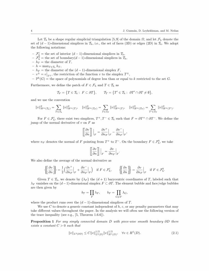
Let Th be a shape regular simplicial triangulation [5,9] of the domain Ω, and let Fh denote theset of (d− 1)-dimensional simplices in Th, i.e., the set of faces (3D) or edges (2D) in Th. We adoptthe following notations:
– F ih = the set of interior (d− 1)-dimensional simplices in Th,– Fbh = the set of boundary(d− 1)-dimensional simplices in Th,– hT = the diameter of T ,– h = maxT∈Th
hT ,– hF = the diameter of the (d− 1)-dimensional simplex F ,– v± = v
∣∣T±
, the restriction of the function v to the simplex T±,– Pk(G) = the space of polynomials of degree less than or equal to k restricted to the set G.
Furthermore, we define the patch of F ∈ Fh and T ∈ Th as
TF =T ∈ Th : F ⊂ ∂T
, TT =
T ′ ∈ Th : ∂T ′ ∩ ∂T 6= ∅
,
and we use the convention
‖v‖2Hm(Th) =∑T∈Th
‖v‖2Hm(T ), ‖v‖2Hm(TF ) =∑T∈TF
‖v‖2Hm(T ), ‖v‖2Hm(TT ) =∑T ′∈TT
‖v‖2Hm(T ′).
For F ∈ F ih, there exist two simplices, T+, T− ∈ Th such that F = ∂T+ ∩ ∂T−. We define thejump of the normal derivative of v on F as[[
∂v
∂n
]] ∣∣∣F
=∂v+
∂nF
∣∣∣F− ∂v−
∂nF
∣∣∣F,
where nF denotes the normal of F pointing from T+ to T−. On the boundary F ∈ Fbh, we take[[∂v
∂n
]] ∣∣∣F
=∂v
∂nF
∣∣∣F.
We also define the average of the normal derivative as∂v
∂n
=
12
( ∂v+
∂nF
∣∣∣F
+∂v−
∂nF
∣∣∣F
)if F ∈ F ih,
∂v
∂n
=
∂v
∂nF
∣∣∣F
if F ∈ Fbh.
Given T ∈ Th, we denote by λF the (d + 1) barycentric coordinates of T , labeled such thatλF vanishes on the (d−1)-dimensional simplex F ⊂ ∂T . The element bubble and face/edge bubblesare then given by
bT =∏F
λF , bF =∏G 6=F
λG,
where the product runs over the (d− 1)-dimensional simplices of T .We use C to denote a generic constant independent of h, ε, or any penalty parameters that may
take different values throughout the paper. In the analysis we will often use the following version ofthe trace inequality (see e.g., [5, Theorem 1.6.6]).
Proposition 1 For any simply connected domain D with piece-wise smooth boundary ∂D thereexists a constant C > 0 such that
‖v‖L2(∂D) ≤ C‖v‖1/2L2(D)‖v‖
1/2H1(D), ∀v ∈ H1(D). (2.1)
Non-conforming elements for a fourth order problem 5
In particular, by a standard scaling argument we obtain the following estimates on any simplex T
‖v‖L2(∂T ) ≤ C(h−1/2T ‖v‖L2(T ) + ‖v‖1/2L2(T )‖∇v‖
1/2L2(T )), ∀v ∈ H1(T ), (2.2a)
‖v‖L2(∂T ) ≤ C(h−1/2T ‖v‖L2(T ) + h
1/2T ‖∇v‖L2(T )), ∀v ∈ H1(T ). (2.2b)
In addition we will also need a standard inverse estimate. Let q be fixed. Then for all v ∈ Pq(T ),
‖v‖L2(∂T ) ≤ Ch−1/2T ‖v‖L2(T ), (2.3)
where C is independent of v.
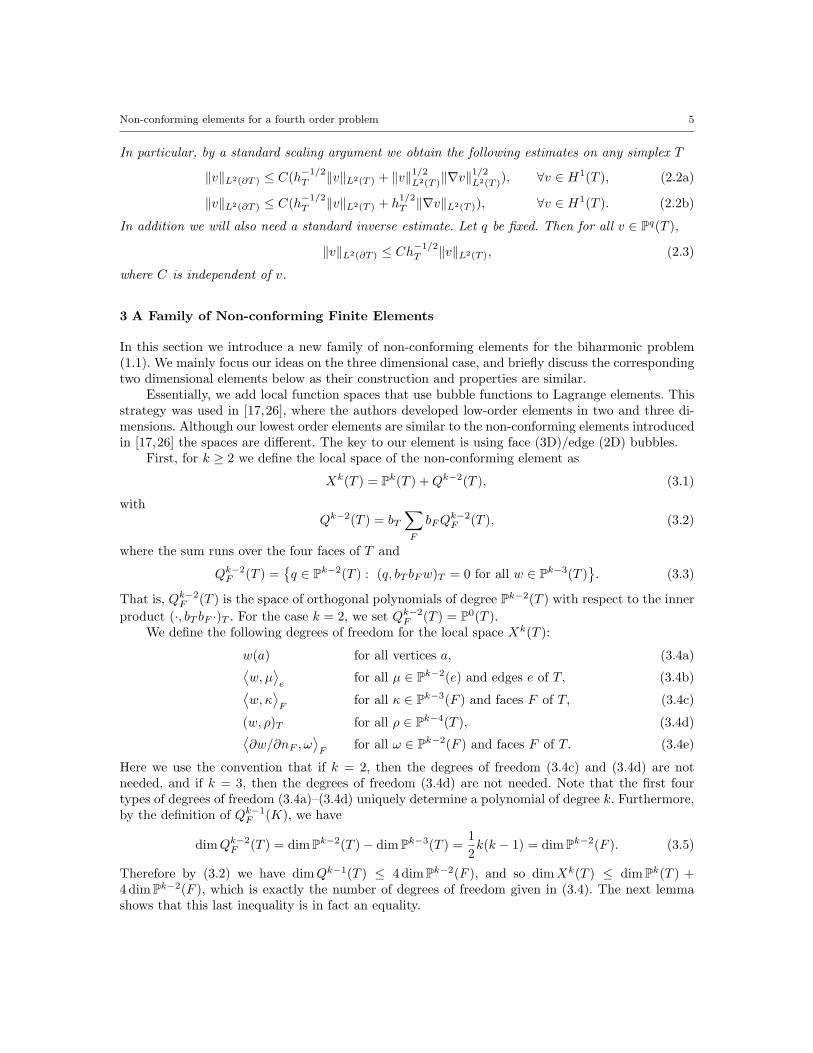
3 A Family of Non-conforming Finite Elements
In this section we introduce a new family of non-conforming elements for the biharmonic problem(1.1). We mainly focus our ideas on the three dimensional case, and briefly discuss the correspondingtwo dimensional elements below as their construction and properties are similar.
Essentially, we add local function spaces that use bubble functions to Lagrange elements. Thisstrategy was used in [17,26], where the authors developed low-order elements in two and three di-mensions. Although our lowest order elements are similar to the non-conforming elements introducedin [17,26] the spaces are different. The key to our element is using face (3D)/edge (2D) bubbles.
First, for k ≥ 2 we define the local space of the non-conforming element as
Xk(T ) = Pk(T ) +Qk−2(T ), (3.1)
withQk−2(T ) = bT
∑F
bFQk−2F (T ), (3.2)
where the sum runs over the four faces of T and
Qk−2F (T ) =
q ∈ Pk−2(T ) : (q, bT bFw)T = 0 for all w ∈ Pk−3(T )
. (3.3)
That is, Qk−2F (T ) is the space of orthogonal polynomials of degree Pk−2(T ) with respect to the inner
product (·, bT bF ·)T . For the case k = 2, we set Qk−2F (T ) = P0(T ).
We define the following degrees of freedom for the local space Xk(T ):
w(a) for all vertices a, (3.4a)⟨w, µ
⟩e
for all µ ∈ Pk−2(e) and edges e of T, (3.4b)⟨w, κ
⟩F
for all κ ∈ Pk−3(F ) and faces F of T, (3.4c)
(w, ρ)T for all ρ ∈ Pk−4(T ), (3.4d)⟨∂w/∂nF , ω
⟩F
for all ω ∈ Pk−2(F ) and faces F of T. (3.4e)
Here we use the convention that if k = 2, then the degrees of freedom (3.4c) and (3.4d) are notneeded, and if k = 3, then the degrees of freedom (3.4d) are not needed. Note that the first fourtypes of degrees of freedom (3.4a)–(3.4d) uniquely determine a polynomial of degree k. Furthermore,by the definition of Qk−1
F (K), we have
dimQk−2F (T ) = dim Pk−2(T )− dim Pk−3(T ) =
12k(k − 1) = dim Pk−2(F ). (3.5)
Therefore by (3.2) we have dimQk−1(T ) ≤ 4 dim Pk−2(F ), and so dimXk(T ) ≤ dim Pk(T ) +4 dim Pk−2(F ), which is exactly the number of degrees of freedom given in (3.4). The next lemmashows that this last inequality is in fact an equality.
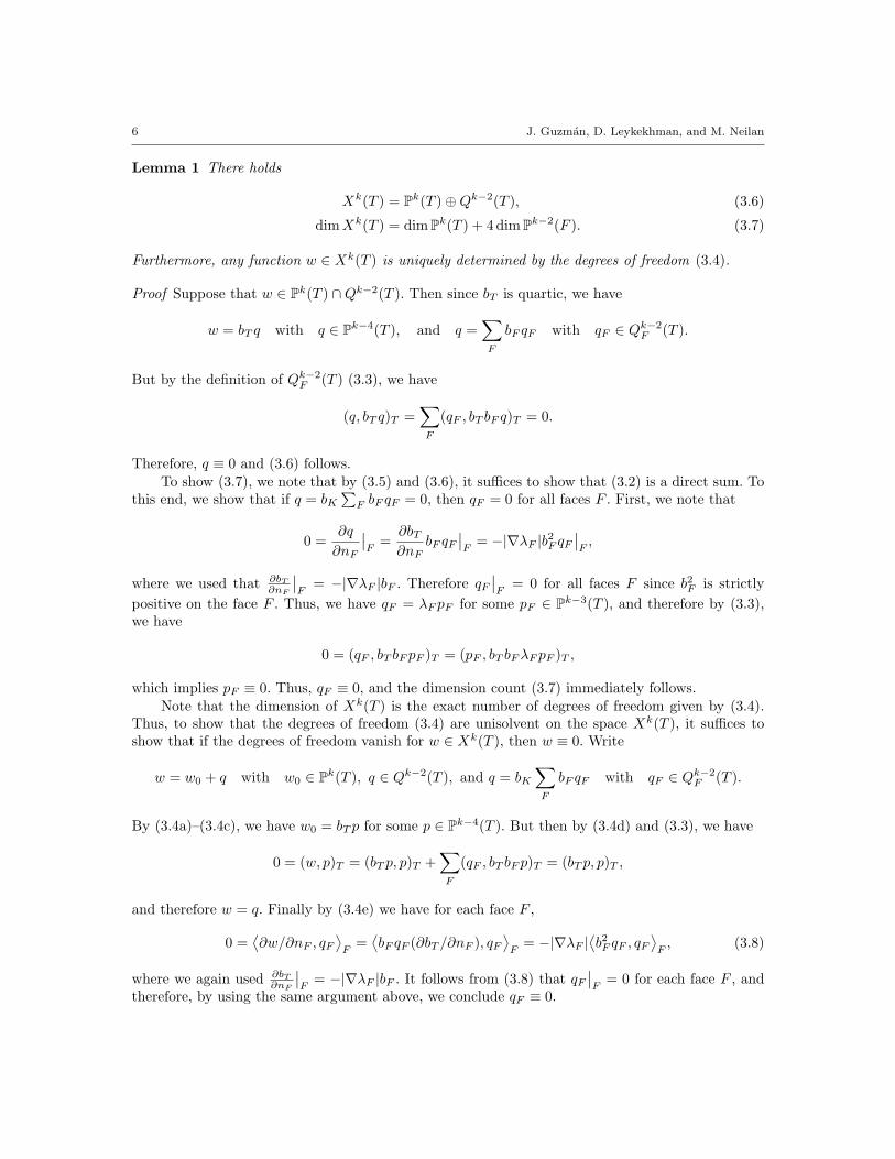
6 J. Guzman, D. Leykekhman, and M. Neilan
Lemma 1 There holds
Xk(T ) = Pk(T )⊕Qk−2(T ), (3.6)
dimXk(T ) = dim Pk(T ) + 4 dim Pk−2(F ). (3.7)
Furthermore, any function w ∈ Xk(T ) is uniquely determined by the degrees of freedom (3.4).
Proof Suppose that w ∈ Pk(T ) ∩Qk−2(T ). Then since bT is quartic, we have
w = bT q with q ∈ Pk−4(T ), and q =∑F
bF qF with qF ∈ Qk−2F (T ).
But by the definition of Qk−2F (T ) (3.3), we have
(q, bT q)T =∑F
(qF , bT bF q)T = 0.
Therefore, q ≡ 0 and (3.6) follows.To show (3.7), we note that by (3.5) and (3.6), it suffices to show that (3.2) is a direct sum. To
this end, we show that if q = bK∑F bF qF = 0, then qF = 0 for all faces F . First, we note that
0 =∂q
∂nF
∣∣F
=∂bT∂nF
bF qF∣∣F
= −|∇λF |b2F qF∣∣F,
where we used that ∂bT
∂nF
∣∣F
= −|∇λF |bF . Therefore qF∣∣F
= 0 for all faces F since b2F is strictlypositive on the face F . Thus, we have qF = λF pF for some pF ∈ Pk−3(T ), and therefore by (3.3),we have
0 = (qF , bT bF pF )T = (pF , bT bFλF pF )T ,
which implies pF ≡ 0. Thus, qF ≡ 0, and the dimension count (3.7) immediately follows.Note that the dimension of Xk(T ) is the exact number of degrees of freedom given by (3.4).
Thus, to show that the degrees of freedom (3.4) are unisolvent on the space Xk(T ), it suffices toshow that if the degrees of freedom vanish for w ∈ Xk(T ), then w ≡ 0. Write
w = w0 + q with w0 ∈ Pk(T ), q ∈ Qk−2(T ), and q = bK∑F
bF qF with qF ∈ Qk−2F (T ).
By (3.4a)–(3.4c), we have w0 = bT p for some p ∈ Pk−4(T ). But then by (3.4d) and (3.3), we have
0 = (w, p)T = (bT p, p)T +∑F
(qF , bT bF p)T = (bT p, p)T ,
and therefore w = q. Finally by (3.4e) we have for each face F ,
0 =⟨∂w/∂nF , qF
⟩F
=⟨bF qF (∂bT /∂nF ), qF
⟩F
= −|∇λF |⟨b2F qF , qF
⟩F, (3.8)
where we again used ∂bT
∂nF
∣∣F
= −|∇λF |bF . It follows from (3.8) that qF∣∣F
= 0 for each face F , andtherefore, by using the same argument above, we conclude qF ≡ 0.
Non-conforming elements for a fourth order problem 7
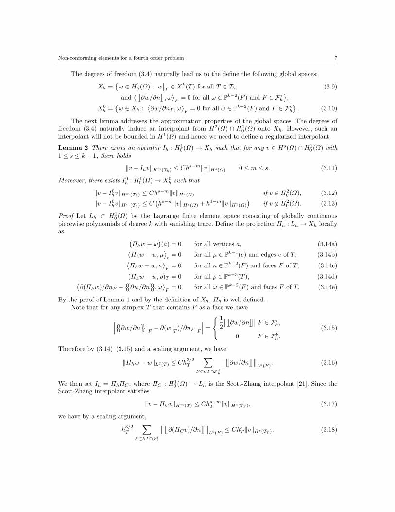
The degrees of freedom (3.4) naturally lead us to the define the following global spaces:
Xh =w ∈ H1
0 (Ω) : w∣∣T∈ Xk(T ) for all T ∈ Th, (3.9)
and⟨[[∂w/∂n
]], ω⟩F
= 0 for all ω ∈ Pk−2(F ) and F ∈ F ih,
X0h =
w ∈ Xh :
⟨∂w/∂nF , ω
⟩F
= 0 for all ω ∈ Pk−2(F ) and F ∈ Fbh. (3.10)
The next lemma addresses the approximation properties of the global spaces. The degrees offreedom (3.4) naturally induce an interpolant from H2(Ω) ∩ H1
0 (Ω) onto Xh. However, such aninterpolant will not be bounded in H1(Ω) and hence we need to define a regularized interpolant.
Lemma 2 There exists an operator Ih : H10 (Ω) → Xh such that for any v ∈ Hs(Ω) ∩H1
0 (Ω) with1 ≤ s ≤ k + 1, there holds
‖v − Ihv‖Hm(Th) ≤ Chs−m‖v‖Hs(Ω) 0 ≤ m ≤ s. (3.11)
Moreover, there exists I0h : H1
0 (Ω)→ X0h such that
‖v − I0hv‖Hm(Th) ≤ Chs−m‖v‖Hs(Ω) if v ∈ H2
0 (Ω), (3.12)
‖v − I0hv‖Hm(Th) ≤ C
(hs−m‖v‖Hs(Ω) + h1−m‖v‖H1(Ω)
)if v 6∈ H2
0 (Ω). (3.13)
Proof Let Lh ⊂ H10 (Ω) be the Lagrange finite element space consisting of globally continuous
piecewise polynomials of degree k with vanishing trace. Define the projection Πh : Lh → Xh locallyas (
Πhw − w)(a) = 0 for all vertices a, (3.14a)⟨
Πhw − w, µ⟩e
= 0 for all µ ∈ Pk−1(e) and edges e of T, (3.14b)⟨Πhw − w, κ
⟩F
= 0 for all κ ∈ Pk−2(F ) and faces F of T, (3.14c)
(Πhw − w, ρ)T = 0 for all ρ ∈ Pk−3(T ), (3.14d)⟨∂(Πhw)/∂nF −
∂w/∂n
, ω⟩F
= 0 for all ω ∈ Pk−2(F ) and faces F of T. (3.14e)
By the proof of Lemma 1 and by the definition of Xh, Πh is well-defined.Note that for any simplex T that contains F as a face we have
∣∣∣∂w/∂n∣∣F− ∂(w
∣∣T
)/∂nF∣∣F
∣∣∣ =
12
∣∣[[∂w/∂n]]∣∣ F ∈ F ih,0 F ∈ Fbh.
(3.15)
Therefore by (3.14)–(3.15) and a scaling argument, we have
‖Πhw − w‖L2(T ) ≤ Ch3/2T
∑F⊂∂T∩Fi
h
∥∥[[∂w/∂n]]∥∥L2(F )
. (3.16)
We then set Ih = ΠhΠC , where ΠC : H10 (Ω) → Lh is the Scott-Zhang interpolant [21]. Since the
Scott-Zhang interpolant satisfies
‖v −ΠCv‖Hm(T ) ≤ Chs−mT ‖v‖Hs(TT ), (3.17)
we have by a scaling argument,
h3/2T
∑F⊂∂T∩Fi
h
∥∥[[∂(ΠCv)/∂n]]∥∥
L2(F )≤ ChsT ‖v‖Hs(TT ). (3.18)
8 J. Guzman, D. Leykekhman, and M. Neilan
Therefore by (3.16)–(3.18) and an inverse estimate, we obtain
‖v − Ihv‖Hm(T ) ≤ ‖v −ΠCv‖Hm(T ) + ‖ΠCv −ΠhΠCv‖Hm(T )
≤ Chs−mT ‖v‖Hs(TT ) + Ch3/2−mT
∑F⊂∂T∩Fi
h
∥∥[[∂(ΠCv)/∂n]]∥∥
L2(F )
≤ Chs−mT ‖v‖Hs(TT ).
To construct an interpolant I0hv in X0
h, we modify the construction of Πh by replacing (3.14e) with
⟨∂(Πhw)/∂nF −
∂w/∂n
, ω⟩F
= 0 for all ω ∈ Pk−2(F ) and interior faces F of T, (3.14e′)⟨∂(Πhw)/∂nF , ω
⟩F
= 0 for all ω ∈ Pk−2(F ) and boundary faces F of T.
If we recall (3.15) for interior faces F and use the fact that
⟨∂(Πhw − w)/∂nF , ω
⟩F
= −⟨∂w/∂nF , ω
⟩F
for all ω ∈ Pk−2(F ) and boundary faces F of T.
We then have
‖Πhw − w‖L2(T ) ≤ Ch3/2T
∑F⊂∂T
∥∥[[∂w/∂n]]∥∥L2(F )
. (3.19)
Note that, in contrast to (3.16), the right-hand side of (3.19) may include boundary faces. However,we see that if v ∈ H2
0 (Ω), then the estimate (3.18) still holds with the sum taken over all faces of T(and not just interior faces). It then follows by using the same argument as above, that if v ∈ H2
0 (Ω),then
‖v − I0hv‖Hm(T ) ≤ Chs−mT ‖v‖Hs(TT ).
However, if v 6∈ H20 (Ω) then we only obtain the estimate
h3/2T
∑F⊂∂T∩Fb
h
∥∥[[∂(ΠCv)/∂n]]∥∥
L2(F )≤ ChT ‖v‖H1(TT ).
It then follows that
‖v − I0hv‖Hm(T ) ≤ ‖v −ΠCv‖Hm(T ) + ‖ΠCv −ΠhΠCv‖Hm(T )
≤ Chs−mT ‖v‖Hs(TT ) + Ch3/2−mT
∑F⊂∂T
∥∥[[∂(ΠCv)/∂n]]∥∥
L2(F )
≤ C(hs−mT ‖v‖Hs(TT ) + h1−m
T ‖v‖H1(TT )
).
Remark 1 The lackluster estimate (3.13) will play a key role while discussing the advantages ofenforcing boundary conditions weakly into the formulation (cf. Remark 3).
Non-conforming elements for a fourth order problem 9
3.1 Remarks on the two dimensional elements
The family of two dimensional elements are similar to the three dimensional case, so we only sketchthe details. The local space of the two dimensional element takes the same form as (3.1), but thesum in (3.2) now run over all edges. Also note that the definition of bF in (3.2)–(3.3) are quadraticedge bubbles instead of cubic face bubbles.
The associated degrees of freedom of Xk(T ) are defined as follows:
w(a) for all vertices a of T, (3.20a)⟨w, µ
⟩F
for all µ ∈ Pk−2(F ) and edges F of T, (3.20b)
(w, ρ)T for all ρ ∈ Pk−3(T ), (3.20c)⟨∂w/∂nF , ω
⟩F
for all ω ∈ Pk−2(F ) and edges F of T. (3.20d)
Lemma 3 There holds
Xk(T ) = Pk(T )⊕Qk−2(T ), (3.21)
dimXk(T ) = dim Pk(T ) + 3Pk−2(F ). (3.22)
Furthermore, any function w ∈ Xk(T ) is uniquely determined by the degrees of freedom (3.20).
The proof of Lemma 3 is very similar to that of Lemma 1, so we omit it. Similar to the threedimensional case, we can define the global spaces as (3.9)–(3.10) by substituting faces by edges inthe definition. Moreover, following similar arguments to those found in the proof of Lemma 2, thereexists interpolants Ih : H1
0 (Ω) → Xh and I0h : H1
0 (Ω) → X0h such that the estimates (3.11)–(3.13)
hold. Again, we omit the proof.
4 The finite element method
In this section we define the finite element method for (1.1) and analyze its convergence. First weprovide the variational form of the singular biharmonic problem. A function u ∈ H2
0 (Ω) is a solutionto (1.1) if for all test functions v ∈ H2
0 (Ω), there holds
Aε(u, v) = (f, v), (4.1)
whereAε(u, v) := ε2a(u, v) + b(u, v), (4.2)
witha(u, v) := (D2u,D2v), b(u, v) := (∇u,∇v). (4.3)
Here, we have used the notation
(D2u,D2v) =∫Ω
D2u : D2v dx =d∑
i,j=1
∫Ω
∂2u
∂xi∂xj
∂2v
∂xi∂xjdx,
and
(∇u,∇v) =∫Ω
∇u · ∇v dx =d∑i=1
∫Ω
∂u
∂xi
∂v
∂xidx.
10 J. Guzman, D. Leykekhman, and M. Neilan
Similarly, a function u ∈ H10 (Ω) is defined to be a solution to (1.3) if there holds
b(u, v) =∫Ω
fv dx ∀v ∈ H10 (Ω). (4.4)
Before continuing, we first state the following a priori estimates and convergence rates to the reducedproblem.
Lemma 4 Let u be the solution to (4.2), and u the solution to the reduced problem (1.3). Thenu ∈ H3(Ω), and there exists a constant C > 0 independent of ε, u, and f such that
‖u‖Hs(Ω) ≤ Cε3/2−s‖f‖L2(Ω) s = 2, 3, (4.5a)
‖u− u‖H1(Ω) ≤ Cε1/2‖f‖L2(Ω), (4.5b)‖u− u‖L2(Ω) ≤ Cε‖f‖L2(Ω). (4.5c)
Proof The proofs of the estimates (4.5a)–(4.5b) are given in [17]. To prove (4.5c), we use a dualityargument. For arbitrary v ∈ L2(Ω), let ψ be the solution to the following second order problem:
−∆ψ = v in Ω, (4.6a)ψ = 0 on ∂Ω. (4.6b)
By (4.6), (1.1), (1.3), and integration by parts, we have
(u− u, v) = b(u− u, ψ) = −ε2a(u, ψ) + ε2⟨∂2u
∂n2
∂ψ
∂n
⟩∂Ω.
Therefore by the trace inequality (2.1), the estimates (4.5a) and elliptic regularity, we obtain
(u− u, v) ≤ Cε2(‖u‖H2(Ω) + ‖u‖1/2H2(Ω)‖u‖
1/2H3(Ω)
)‖ψ‖H2(Ω)
≤ Cε2(ε−1/2 +
(ε−1/2
)1/2(ε−3/2
)1/2)‖f‖L2(Ω)‖v‖L2(Ω)
≤ Cε‖f‖L2(Ω)‖v‖L2(Ω).
The estimate (4.5c) then follows from this last inequality.
To define the finite element method, we introduce the bilinear form
ah(v, w) =∑T∈Th
(D2v,D2w)T −∑F∈Fb
h
⟨ ∂2v
∂n2F
,∂w
∂nF
⟩F
(4.7)
−∑F∈Fb
h
⟨ ∂v
∂nF,∂2w
∂n2F
⟩F
+ σ∑F∈Fb
h
h−1F
⟨ ∂v
∂nF,∂w
∂nF
⟩F,
where σ is a positive penalization parameter. Although, theoretically σ needs to be sufficiently largeto ensure the stability of the method (cf. Lemma 5 below), our numerical examples show that themethod is robust even for very small values of σ, even for σ = 0 (cf. Section 8).
The finite element method then reads: Find uh ∈ Xh such that
Aε,h(uh, w) = (f, w) ∀w ∈ Xh, (4.8)
whereAε,h(w, v) = ε2ah(w, v) + b(w, v). (4.9)
Non-conforming elements for a fourth order problem 11
We define the following norms associated with problem (4.8):
‖v‖22,h =∑T∈Th
|v|2H2(T ) +∑F∈Fb
h
h−1F ‖∂v/∂nF ‖
2L2(F ), (4.10)
‖v‖2ε,h = ε2‖v‖22,h + |v|2H1(Ω). (4.11)
The next lemma shows that the finite element method (4.8) is well-posed.
Lemma 5 There exists a constant σ0 > 0 depending only on the shape regularity of Th, such thatfor σ ≥ σ0, there holds
12‖w‖2ε,h ≤ Aε,h(w,w) ∀w ∈ Xh. (4.12)
Proof To show (4.12), it suffices to show that the bilinear form ah(·, ·) is coercive with respect tothe norm ‖ · ‖2,h. By the form’s definition (4.7), we have
ah(w,w) =∑T∈Th
|w|2H2(T ) − 2∑F∈Fb
h
⟨∂2w/∂n2
F , ∂w/∂nF⟩F
+ σ∑F∈Fb
h
h−1F ‖∂w/∂nF ‖
2L2(F ). (4.13)
By the Cauchy-Schwarz inequality and a standard scaling argument, there exists a constant C > 0depending only on the shape regularity of the mesh such that
2∑F∈Fb
h
⟨∂2w/∂n2
F , ∂w/∂nF⟩F≤ 2
∑F∈Fb
h
hF ‖∂2w/∂n2F ‖2L2(F )
1/2 ∑F∈Fb
h
h−1F ‖∂w/∂nF ‖
2L2(F )
1/2
≤ C
∑F∈Fb
h
|w|2H2(TF )
1/2 ∑F∈Fb
h
h−1F ‖∂w/∂nF ‖
2L2(F )
1/2
≤ 12
∑T∈Th
|w|2H2(T ) +C2
2
∑F∈Fb
h
h−1F ‖∂w/∂nF ‖
2L2(F ).
Therefore by (4.13) we obtain
ah(w,w) ≥ 12
∑T∈Th
|w|2H2(T ) +(σ − C2
2) ∑F∈Fi
h
h−1F ‖∂w/∂nF ‖
2L2(F ).
Choosing σ0 = 12 (C2 + 1), we obtain (4.12).
Before deriving our main results, we need a few more technical lemmas. The first measures theinterpolation error in the norm given by (4.11).
Lemma 6 Let u ∈ Hs(Ω) with 3 ≤ s ≤ k + 1 be the solution to (1.1), and let Ih be the interpolantfrom Lemma 2. Then there holds
‖u− Ihu‖ε,h ≤ C(hs−1 + εhs−2
)‖u‖Hs(Ω), (4.14a)
‖u− Ihu‖ε,h ≤ Ch1/2‖f‖L2(Ω). (4.14b)
Moreover, if the solution to the reduced problem satisfies u ∈ Hm(Ω) for some 2 ≤ m ≤ k + 1, then
‖u− Ihu‖ε,h ≤ C(ε1/2‖f‖L2(Ω) + hm−1‖u‖Hm(Ω)
). (4.14c)
12 J. Guzman, D. Leykekhman, and M. Neilan
Proof By (3.11) and (4.5a), we have
ε2∑T∈Th
|u− Ihu|2H2(T ) ≤ Cε2h2s−4‖u‖2Hs(Ω), (4.15a)
ε2∑T∈Th
|u− Ihu|2H2(T ) ≤ Cε2h‖u‖H2(Ω)‖u‖H3(Ω) ≤ Ch‖f‖2L2(Ω), (4.15b)
and
ε2∑T∈Th
|u− Ihu|2H2(T ) ≤ Cε2‖u‖2H2(Ω) ≤ Cε‖f‖
2L2(Ω). (4.15c)
Similarly, we have by (3.11), (4.5a), and the trace inequality (2.2b),
ε2∑F∈Fb
h
h−1F
∥∥∂(u− Ihu)/∂nF∥∥2
L2(F )≤ Cε2
∑T∈Th
(h−2T ‖u− Ihu‖
2H1(T ) + ‖u− Ihu‖2H2(T )
)(4.16a)
≤ Cε2h2s−4‖u‖2Hs(Ω),
ε2∑F∈Fb
h
h−1F
∥∥∂(u− Ihu)/∂nF∥∥2
L2(F )≤ Cε2
∑T∈Th
(h−2T ‖u− Ihu‖
2H1(T ) + ‖u− Ihu‖2H2(T )
)(4.16b)
≤ Cε2h‖u‖H2(Ω)‖u‖H3(Ω) ≤ Ch‖f‖2L2(Ω),
and
ε2∑F∈Fb
h
h−1F
∥∥∂(u− Ihu)/∂nF∥∥2
L2(F )≤ Cε2
∑T∈Th
(h−2T ‖u− Ihu‖
2H1(T ) + ‖u− Ihu‖2H2(T )
)(4.16c)
≤ Cε2‖u‖2H2(Ω) ≤ Cε‖f‖2L2(Ω).
Moreover, we have by (3.11), (4.5a), (4.5b), and (1.4),
|u− Ihu|2H1(Ω) ≤ Ch2s−2‖u‖2Hs(Ω), (4.17a)
|u− Ihu|2H1(Ω) ≤ C(|u− u− Ih(u− u)|2H1(Ω) + |u− Ihu|2H1(Ω)
)(4.17b)
≤ C(h‖u− u‖H1(Ω)‖u− u‖H2(Ω) + h2‖u‖2H2(Ω)
)≤ Ch‖f‖2L2(Ω)
and
|u− Ihu|2H1(Ω) ≤ C(|u− u− Ih(u− u)|2H1(Ω) + |u− Ihu|2H1(Ω)
)(4.17c)
≤ C(‖u− u‖2H1(Ω) + h2m−2‖u‖2Hm(Ω)
)≤ C
(ε‖f‖2L2(Ω) + h2m−2‖u‖2Hm(Ω)
).
The first estimate (4.14a) then follows from (4.11), (4.15a), (4.16a) and (4.17a); the secondestimate (4.14b) follows from (4.11), (4.15b), (4.16b) and (4.17b); and the third estimate (4.14c)follows from (4.11), (4.15c), (4.16c) and (4.17c).
The next lemma is needed to analyze the error equation. It provides bounds for the interpolationerror in the bilinear form restricted to the subspace.
Non-conforming elements for a fourth order problem 13
Lemma 7 Under the same hypotheses of Lemma 6, for any w ∈ Xh there holds,
Aε,h(u− Ihu,w) ≤ C(1 + σ)(hs−1 + εhs−2
)‖u‖Hs(Ω)‖w‖ε,h, (4.18a)
Aε,h(u− Ihu,w) ≤ C(1 + σ)h1/2‖f‖L2(Ω)‖w‖ε,h, (4.18b)
Aε,h(u− Ihu,w) ≤ C(1 + σ)(ε1/2‖f‖L2(Ω) + hm−1‖u‖Hm(Ω)
)‖w‖ε,h. (4.18c)
Proof By (4.9), we have
Aε,h(u− Ihu,w) = ε2∑T∈Th
(D2(u− Ihu), D2w)T + (∇(u− Ihu),∇w) (4.19)
− ε2∑F∈Fb
h
⟨∂2(u− Ihu)∂n2
F
∂w
∂nF
⟩F− ε2
∑F∈Fb
h
⟨∂(u− Ihu)∂nF
,∂2w
∂n2F
⟩F
+ ε2σ∑F∈Fb
h
h−1F
⟨∂(u− Ihu)∂nF
,∂w
∂nF
⟩F
=: J1 + J2 + J3 + J4 + J5.
By the Cauchy-Schwarz inequality, (2.3) and (4.11), we can show
J1, J2, J4, J5 ≤ C(1 + σ)‖u− Ihu‖ε,h‖w‖ε,h.
Using (4.14) we have
J1, J2, J4, J5 ≤ C(1 + σ)(εhs−2 + hs−1)‖u‖Hs(Ω)‖w‖ε,h, (4.20a)
J1, J2, J4, J5 ≤ C(1 + σ)h1/2‖f‖L2(Ω)‖w‖ε,h, (4.20b)
and
J1, J2, J4, J5 ≤ C(1 + σ)(ε1/2‖f‖L2(Ω) + hm−1‖u‖Hm(Ω)
)‖w‖ε,h. (4.20c)
Next, by the Cauchy-Schwarz inequality, the trace inequality (2.2b), (4.11) and (3.11), we have
J3 ≤ Cε2 ∑F∈Fb
h
hF ‖∂2(u− Ihu)/∂n2F ‖2L2(F )
1/2 ∑F∈Fb
h
h−1F ‖∂w/∂nF ‖
2L2(F )
1/2
(4.21a)
≤ Cε
(∑T∈Th
(‖u− Ihu‖2H2(T ) + h2
T ‖u− Ihu‖2H3(T )
))1/2
‖w‖ε,h
≤ Cεhs−2‖u‖Hs(Ω)‖w‖ε,h.
Furthermore, by the trace inequality (2.2b), (3.11), the inverse estimate (2.3), and (4.5a), we have
J3 ≤ Cε2(∑T∈Th
(h−2T ‖u− Ihu‖
2H2(T ) + ‖u− Ihu‖2H3(T )
))1/2
‖w‖H1(T ) (4.20c)
≤ Cε2‖u‖H3(Ω)‖w‖ε,h ≤ Cε1/2‖f‖L2(Ω)‖w‖ε,h.
14 J. Guzman, D. Leykekhman, and M. Neilan
Note that if ε ≤ h, then this last estimate also implies
J3 ≤ Ch1/2‖f‖L2(Ω)‖w‖ε,h. (4.20b′)
On the other hand, if h ≤ ε we can use (4.21a) with s = 3 and (4.5a) to obtain
J3 ≤ Cεh‖u‖H3(Ω)‖w‖ε,h ≤ Ch1/2‖f‖L2(Ω)‖w‖ε,h. (4.20b′′)
Finally, the estimate (4.18a) follows from (4.19), (4.20a) and (4.21a); the second estimate (4.18b)follows from (4.19), (4.20b) and (4.20b); and the third estimate (4.18c) follows from (4.19), (4.20c)and (4.20c).
We now are now in position to state the prove the main result of this section.
Theorem 1 Suppose that u ∈ Hs(Ω) with 3 ≤ s ≤ k+1. Then there exists a constant C independentof ε and h such that
‖u− uh‖ε,h ≤ C(εhs−2 + hs−1)‖u‖Hs(Ω), (4.22a)
‖u− uh‖ε,h ≤ Ch1/2‖f‖L2(Ω). (4.22b)
Moreover, if u ∈ Hm(Ω) with 2 ≤ m ≤ k + 1, then
‖u− uh‖ε,h ≤ C(ε1/2‖f‖L2(Ω) + hm−1‖u‖Hm(Ω)
). (4.22c)
Remark 2 We would like to point out that for ε = o(h) the estimate (4.22c) gives a better orderapproximation than the uniform order h1/2.
Proof Let Ihu be the interpolant of u defined in Lemma 2 and set w = Ihu − uh ∈ Xh. Then by(4.12) and (4.8), we have
12‖w‖ε,h ≤ Aε,h(Ihu− uh, w) = Aε,h(Ihu− u,w) + Eh(u,w), (4.23)
where the consistency error is defined as
Eh(u,w) = Aε,h(u,w)− (f, w) = ε2ah(u,w) + b(u,w)− (f, w). (4.24)
Since u ∈ H3(Ω), equation (1.1) can be considered in the H−1(Ω) sense, and therefore we have
−ε2(∇∆u,∇w) + (∇u,∇w)− (f, w) = 0 ∀w ∈ Xh ⊂ H10 (Ω).
Hence, by (4.24), (1.1b), (4.7) and integration by parts,
Eh(u,w) = ε2∑F∈Fi
h
⟨ ∂2u
∂n2F
,
[[∂w
∂n
]]⟩F. (4.25)
By the definition of Xh (3.9), there holds for any ω ∈ Pk−2(F ),⟨ ∂2u
∂n2F
,
[[∂w
∂n
]]⟩F
=⟨ ∂2u
∂n2F
− ω,[[∂w
∂n
]]⟩F.
Non-conforming elements for a fourth order problem 15
In particular, we have⟨ ∂2u
∂n2F
,
[[∂w
∂n
]]⟩F
=⟨∂2(u−ΠCu)
∂n2
,
[[∂w
∂n
]]⟩F
≤∥∥∂2(u−ΠCu)/∂n2
∥∥L2(F )
∥∥[[∂w/∂n]]∥∥L2(F )
, (4.26)
where we recall that ΠC is the Scott-Zhang interpolant of order k which has the following approxi-mation properties:
‖u−ΠCu‖Hm(Th) ≤ C hs−m‖u‖Hs(Th) for 1 ≤ m ≤ s ≤ k + 1. (4.27)
We bound each of the factors on the right of (4.26) separately. Using that the average of[[∂w∂n
]]vanishes on F we have by Poincare’s inequality that∥∥[[∂w/∂n]]∥∥
L2(F )≤ C hF
∥∥∇F ([[∂w/∂n
]])∥∥L2(F )
,
where ∇F is the surface gradient on F . We then have by the inverse estimate (2.3) that∥∥[[∂w/∂n]]∥∥L2(F )
≤ C h1/2F |w|H2(TF ). (4.28)
Of course, using the inverse estimate (2.3) twice we also have∥∥[[∂w/∂n]]∥∥L2(F )
=∥∥[[∂w/∂n]]∥∥1/2
L2(F )
∥∥[[∂w/∂n]]∥∥1/2
L2(F )≤ C |w|1/2H1(TF )|w|
1/2H2(TF ). (4.29)
Next, using the trace inequality (2.2a) we obtain∥∥∂2(u−ΠCu)/∂n2∥∥
L2(F )(4.30)
≤ C(h−1/2F |u−ΠCu|H2(TF ) + |u−ΠCu|1/2H2(TF )|u−ΠCu|1/2H3(TF )
).
Using (4.26), (4.28), (4.30) and (4.27) we obtain
Eh(u,w) ≤ C εhs−2‖u‖Hs(Ω)‖w‖ε,h. (4.31)
The error estimate (4.22a) then follows from (4.23), (4.18a), (4.31), the triangle inequality and(4.14a).
Alternatively, by (4.26), (4.28), (4.30), (4.27) and (4.5a) we get
Eh(u,w) ≤ C εh1/2‖u‖1/2H3(Ω)‖u‖1/2H2(Ω)‖w‖ε,h ≤ Ch
1/2‖f‖L2(Ω)‖w‖ε,h. (4.32)
The error estimate (4.22b) follows from (4.23), (4.18b), (4.32) and (4.14b).Finally, by (4.26), (4.29), (4.30), (4.27) and (4.5a) we see that
Eh(u,w) ≤ Cε2‖u‖1/2H3(Ω)‖u‖1/2H2(Ω)|w|
1/2H2(Th)|w|
1/2H1(Ω) (4.33)
≤ Cε3/2‖u‖1/2H3(Ω)‖u‖1/2H2(Ω)‖w‖ε,h ≤ Cε
1/2‖f‖L2(Ω)‖w‖ε,h.
The third estimate (4.22c) is then deduced from (4.23), (4.18c), (4.33) and (4.14c).
16 J. Guzman, D. Leykekhman, and M. Neilan
4.1 Remarks on imposing boundary conditions strongly
Similar to other non-conforming finite element methods (e.g. [15,17,24]), we can define a finiteelement method for (1.1) that imposes the normal derivative boundary conditions strongly in thefinite element space. Although this approach is perhaps more natural than the one proposed above,we argue that the method does not inherit as good convergence properties.
In this case, we define the method as finding u0h ∈ X0
h such that
A0ε,h(u0
h, v) = (f, v) ∀v ∈ X0h, (4.34)
where
A0ε,h(w, v) = ε2
∑T∈Th
(D2w,D2v)T + (∇w,∇v),
and we recall that the finite element space X0h is defined by (3.10).
It is easily to see that (4.34) is well-posed as
‖v‖2A := A0ε,h(v, v) (4.35)
is a norm on X0h. Furthermore, we have the following convergence result.
Theorem 2 Let u ∈ Hs(Ω) with (3 ≤ s ≤ k + 1) be the solution to (1.1), and let u0h ∈ X0
h satisfy(4.34). Then there holds
‖u− u0h‖A ≤ C
(hs−1 + εhs−2
)‖u‖Hs(Ω), (4.36a)
‖u− u0h‖A ≤ Ch1/2‖u‖Hs(Ω). (4.36b)
Proof The proof of Theorem 2 is similar to that of Theorem 1 so we only provide a sketch.First, by the proof of Lemma 6 along with the interpolation estimates (3.12)–(3.13), we have
‖u− I0hu‖A ≤ C
(hs−1 + εhs−2
)‖u‖Hs(Ω), (4.37a)
‖u− I0hu‖A ≤ Ch1/2‖f‖L2(Ω). (4.37b)
Next, setting w = I0hu− u0
h, we have by (4.35) and (4.34),
‖w‖2A = A0ε,h(I0
hu− u,w) + E0h(u,w), (4.38)
where E0h(u,w) = A0
ε,h(u,w)− (f, w).By the proof of Lemma 7 and by (3.12)–(3.13), we have
A0ε,h(u− I0
hu,w) ≤ C(1 + σ)(hs−1 + εhs−2
)‖u‖Hs(Ω)‖w‖A, (4.39a)
A0ε,h(u− I0
hu,w) ≤ C(1 + σ)h1/2‖f‖L2(Ω)‖w‖A. (4.39b)
Next, after integrating by parts, we conclude
E0h(u,w) = ε2
∑F∈Fh
⟨ ∂2u
∂n2F
,
[[∂w
∂n
]]⟩F.
Thus, by using the same arguments in the proof of Theorem 1, we have
E0h(u,w) ≤ C
(hs−1 + εhs−2
)‖u‖Hs(Ω)‖w‖A, (4.40a)
E0h(u,w) ≤ Ch1/2‖f‖L2(Ω)‖w‖A. (4.40b)
The estimate (4.36a) then follows from (4.38), (4.39a), (4.40a) and (4.37a), where as the estimate(4.36b) follows from (4.38), (4.39b), (4.40b) and (4.37b).
Non-conforming elements for a fourth order problem 17
Remark 3 Note that the error u − u0h does not satisfy an estimate of the form (4.22c). This is due
to the fact that we cannot derive an estimate of the interpolation error of the form (4.14c). Bycarefully studying the proof of Lemma 6, we find a problem occurs when we try to estimate the term|u − I0
hu|H1(Ω) due to the interpolation result (3.13). Indeed, in comparison to (4.17c), we have by(3.13) and (4.5a),
|u− I0hu|H1(Ω) ≤ C
(|u− u− I0
h(u− u)|H1(Ω) + |u− I0hu|H1(Ω)
)≤ C
(‖u− u‖H1(Ω) + |u− I0
hu|H1(Ω)
)≤ C
(ε1/2‖f‖L2(Ω) + |u− I0
hu|H1(Ω)
).
However, by (3.13) we can only conclude
|u− I0hu|H1(Ω) ≤ C‖u‖H1(Ω),
and therefore the estimate does not yield anything.From this result, we see the advantages of imposing Neumann boundary conditions weakly. In
particular, if ε h, then by (4.22c) we will observe convergence rates of O(hm−1) in the energynorm instead of convergence rates of O(h1/2).
5 L2 error estimates
In this section we prove error estimates in the L2 norm for ε small relative to h. Again, we see theadvantage of using Nitsche’s method. We also state an ε-independent estimates.
Theorem 3 Let u and uh satisfy (1.1) and (4.8) respectively. Then, for ε ≤ h and for u ∈ Hm(Ω)with 2 ≤ m ≤ k + 1, there exists a constant C such that
‖u− uh‖L2(Ω) ≤ C(1 + σ)2((hε1/2 + ε
)‖f‖L2(Ω) + hm‖u‖Hm(Ω)
).
In particular, we have
‖u− uh‖L2(Ω) ≤ C(1 + σ)2(ε+ h2
)‖f‖L2(Ω).
Proof We can decompose the error as
u− uh = (u− u) + (u− uh). (5.1)
By (4.5b), we have
‖u− u‖L2(Ω) ≤ Cε‖f‖L2(Ω). (5.2)
Thus we only need to estimate ‖u− uh‖L2(Ω).Let z ∈ H1
0 (Ω) be the solution to the following problem:
(∇z,∇w) = (u− uh, w), ∀w ∈ H10 (Ω). (5.3)
We then have
‖u− uh‖2L2(Ω) =(∇(z − Ihz),∇(u− uh)
)+(∇Ihz,∇(u− uh)
)=: J1 + J2. (5.4)
18 J. Guzman, D. Leykekhman, and M. Neilan
By (3.11), the triangle inequality, (4.5b) and (4.11),
J1 ≤ Ch‖u− uh‖H1(Ω)‖z‖H2(Ω) ≤ Ch(ε1/2‖f‖L2(Ω) + ‖u− uh‖ε,h
)‖z‖H2(Ω). (5.5)
To estimate J2 we have by (4.8), (1.3) and (4.7),
J2 = ε2ah(uh, Ihz) (5.6)
= ε2∑T∈Th
(D2uh, D2Ihz)T − ε2
∑F∈Fb
h
⟨ ∂uh∂nF
,∂2Ihz
∂n2F
⟩F
+ ε2σ∑F∈Fb
h
h−1F
⟨ ∂uh∂nF
,∂(Ihz − z)
∂nF
⟩F− ε2
∑F∈Fb
h
⟨∂2uh∂n2
F
,∂(Ihz − z)
∂nF
⟩F
+ ε2σ∑F∈Fb
h
h−1F
⟨ ∂uh∂nF
,∂z
∂nF
⟩F− ε2
∑F∈Fb
h
⟨∂2uh∂n2
F
,∂z
∂nF
⟩F
=: K1 +K2 +K3 +K4 +K5 +K6.
Using the Cauchy-Schwarz, inverse inequalities, (4.5a), (4.22b) and (3.11), we have
K1 ≤ Cε2h−1‖uh‖H1(Ω)‖Ihz‖H2(Th) ≤ Cε‖f‖L2(Ω)‖z‖H2(Ω), (5.7)
where we used that ε ≤ h.Bounding K2 we use that ∂u/∂n = 0 on ∂Ω. Thus by the Cauchy-Schwarz, the inverse inequality
(2.3), and (3.11),
K2 ≤ ε2 ∑F∈Fb
h
h−1F
∥∥∂(u− uh)/∂nF∥∥2
L2(F )
1/2 ∑F∈Fb
h
hF∥∥∂2Ihz/∂n
2F
∥∥2
L2(F )
1/2
(5.8)
≤ Cε‖u− uh‖ε,h‖Ihz‖H2(Th) ≤ Cε‖u− uh‖ε,h‖z‖H2(Ω).
Below we will need the following estimate which follows from the trace inequality (2.2b) and theinterpolation estimate (4.14a)∥∥∂(Ihz − z)/∂n
∥∥L2(∂F )
≤ h1/2‖z‖H2(TF ). (5.9)
We easily see using (5.9) that we have the bound
K3 ≤ Cσε‖u− uh‖ε,h‖z‖H2(Ω). (5.10)
Bounding K4, we have use (5.9) and the inverse estimate (2.3)
K4 ≤ Cε2‖uh‖H2(Th)‖z‖H2(Ω).
Note that by the triangle and inverse inequalities, (3.11), (4.5a) and (4.22b),
‖u− uh‖H2(Th) ≤ ‖u− Ihu‖H2(Th) + h−1‖Ihu− uh‖H1(Ω) (5.11)
≤ C‖u‖H2(Ω) + h−1‖u− uh‖H1(Ω)
≤ C(ε−1/2 + h−1/2
)‖f‖L2(Ω) ≤ Cε−1/2‖f‖L2(Ω)
Non-conforming elements for a fourth order problem 19
since ε ≤ h. Thus, ‖uh‖H2(Th) ≤ Cε−1/2‖f‖L2(Ω), and therefore
K4 ≤ ε3/2‖f‖L2(Ω)‖z‖H2(Ω). (5.12)
Bounding K5, we again use that ∂u/∂n = 0 on ∂Ω. Thus by the Cauchy-Schwarz inequality,the trace inequality (2.2b), the trace inequality (2.1), (5.11), (4.22b), and the fact ε ≤ h,
K5 ≤ σε2 ∑F∈Fb
h
h−2F
∥∥∂(u− uh)/∂nF∥∥2
L2(F )
1/2
‖∂z/∂n‖L2(∂Ω) (5.13)
≤ Cσε2 ∑F∈Fb
h
(h−3F ‖u− uh‖
2H1(TF ) + h−1
F ‖u− uh‖2H2(TF )
)1/2
‖z‖H2(Ω)
≤ Cσε2(h−3/2‖u− uh‖H1(Ω) + h−1/2‖u− uh‖H2(Th)
)‖z‖H2(Ω)
≤ Cσε2(h−1 + h−1/2ε−1/2
)‖f‖L2(Ω)‖z‖H2(Ω)
≤ Cσε‖f‖L2(Ω)‖z‖H2(Ω).
Similarly we can bound K6 as follows
K6 ≤ ε2 ∑F∈Fb
h
‖∂2uh/∂n2F ‖2L2(F )
1/2
‖∂z/∂n‖L2(∂Ω) (5.14)
≤ ε2h−1/2‖uh‖H2(Th)‖z‖H2(Ω) ≤ ε‖f‖L2(Ω)‖z‖H2(Ω),
where again, we used the hypothesis ε ≤ h.Applying the estimates (5.7)–(5.10) and (5.12)–(5.14) to (5.6) we have
J2 ≤ C(1 + σ)(ε‖f‖L2(Ω) + ε‖u− uh‖ε,h
)‖z‖H2(Ω).
Combining this last inequality with (5.5) and (5.4), and using the H2 regularity of z, we conclude
‖u− uh‖L2(Ω) ≤ C(1 + σ)(
(hε1/2 + ε)‖f‖L2(Ω) + (h+ ε)‖u− uh‖ε,h).
It then follows from (5.1), (5.2) and (4.22c) that
‖u− uh‖L2(Ω) ≤ C(1 + σ)(
(hε1/2 + ε)‖f‖L2(Ω) + (h+ ε)‖u− uh‖ε,h)
≤ C(1 + σ)(
(hε1/2 + ε)‖f‖L2(Ω) + h‖u− uh‖ε,h)
≤ C(1 + σ)2(
(hε1/2 + ε)‖f‖L2(Ω) + hm‖u‖Hm(Ω)
).
Next we state an ε-independent estimate.
Theorem 4 Let u and uh satisfy (1.1) and (4.8) respectively. There exists a constant C such that
‖u− uh‖L2(Ω) ≤ Ch ‖f‖L2(Ω).
The proof of Theorem 4 is based on the duality argument
ε2∆z −∆z = u− uh in Ω,
z =∂z
∂n= 0 on ∂Ω,
and by using similar techniques as those found in Theorems 3 and 1. Since the proof is long andsimilar to ones above, we omit it.
20 J. Guzman, D. Leykekhman, and M. Neilan
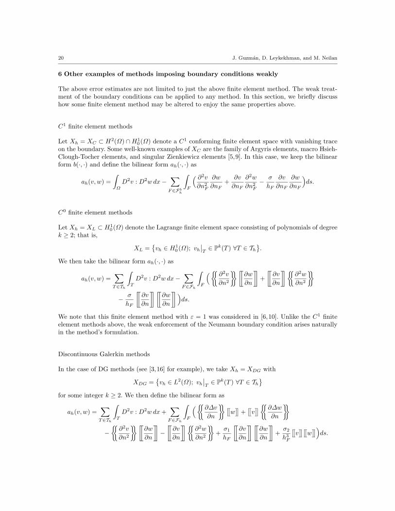
6 Other examples of methods imposing boundary conditions weakly
The above error estimates are not limited to just the above finite element method. The weak treat-ment of the boundary conditions can be applied to any method. In this section, we briefly discusshow some finite element method may be altered to enjoy the same properties above.
C1 finite element methods
Let Xh = XC ⊂ H2(Ω) ∩H10 (Ω) denote a C1 conforming finite element space with vanishing trace
on the boundary. Some well-known examples of XC are the family of Argyris elements, macro Hsieh-Clough-Tocher elements, and singular Zienkiewicz elements [5,9]. In this case, we keep the bilinearform b(·, ·) and define the bilinear form ah(·, ·) as
ah(v, w) =∫Ω
D2v : D2w dx−∑F∈Fb
h
∫F
( ∂2v
∂n2F
∂w
∂nF+
∂v
∂nF
∂2w
∂n2F
− σ
hF
∂v
∂nF
∂w
∂nF
)ds.
C0 finite element methods
Let Xh = XL ⊂ H10 (Ω) denote the Lagrange finite element space consisting of polynomials of degree
k ≥ 2; that is,
XL =vh ∈ H1
0 (Ω); vh∣∣T∈ Pk(T ) ∀T ∈ Th
.
We then take the bilinear form ah(·, ·) as
ah(v, w) =∑T∈Th
∫T
D2v : D2w dx−∑F∈Fh
∫F
( ∂2v
∂n2
[[∂w
∂n
]]+[[∂v
∂n
]]∂2w
∂n2
− σ
hF
[[∂v
∂n
]] [[∂w
∂n
]])ds.
We note that this finite element method with ε = 1 was considered in [6,10]. Unlike the C1 finiteelement methods above, the weak enforcement of the Neumann boundary condition arises naturallyin the method’s formulation.
Discontinuous Galerkin methods
In the case of DG methods (see [3,16] for example), we take Xh = XDG with
XDG =vh ∈ L2(Ω); vh
∣∣T∈ Pk(T ) ∀T ∈ Th
for some integer k ≥ 2. We then define the bilinear form as
ah(v, w) =∑T∈Th
∫T
D2v : D2w dx+∑F∈Fh
∫F
(∂∆v∂n
[[w]]
+[[v]]∂∆w
∂n
−∂2v
∂n2
[[∂w
∂n
]]−[[∂v
∂n
]]∂2w
∂n2
+σ1
hF
[[∂v
∂n
]] [[∂w
∂n
]]+σ2
h3F
[[v]][[
w]])ds.
Non-conforming elements for a fourth order problem 21
We also replace the bilinear form b(·, ·) with
bh(v, w) =∑T∈Th
∫T
∇v · ∇w dx−∑F∈Fh
( ∂v∂n
[[w]]
+[[v]]∂w
∂n
− σ3
hF
[[v]][[
w]])ds.
In comparison to other methods, both boundary conditions are imposed weakly. Our analysis showsthat there is no obvious advantages to imposing function values on the boundary weakly for theproblem in hand.
7 Discussion on local error estimates and pollution effects
In this section we discuss the local error estimates and a pollution effect from the boundary layers.Our analysis above shows that for ε small the presence of boundary layers has a substantial effecton global a priori error estimates when the Neumann boundary conditions are imposed strongly (cf.Section 4.1). As a result, the use of high order elements do not necessary improve the convergencerates. On the other hand, since the boundary layers are contained in a small neighborhood of theboundary, one would expect better convergence rates in the interior of the domain. However as wasshown in [22,23] for conformal C1 elements, the improvement is only minor. In those papers, Sempershowed that for ε < h the presence of boundary layers pollutes the finite element method everywhereeven far away from the boundary, and that the error in the interior is controlled by the global errorin the L2 norm; this error happens to be of order h. Numerical results using C1 Hermite polynomialsin one dimension presented in those papers confirm this statement (cf. Table 2 and 3 in [23]). Westress that this strong pollution effect is not due to the fact that C1 basis are used, but due to thetreatment of Neumann boundary conditions strongly.
The above result may look surprising if compared to analogous result of singularly perturbedreaction-diffusion problem,
−ε2∆u+ u = f in Ω, (7.1a)u = 0 on ∂Ω. (7.1b)
Indeed, Schatz and Wahlbin [19], proved that the standard conformal finite element approximationto the above problem converges optimally on any interior subdomain; i.e., there is no pollution fromthe boundary layers into the interior.
At first glance this may seem puzzling since both problems are singularly perturbed ellipticproblems, but their conformal finite elements behave so differently. The fundamental issue lies in thedifference between the low order terms of each respective equation and its Galerkin approximation(i.e. difference between the Ritz and L2 projections). Some additional insight to that phenomenacan be obtained from looking at one dimensional problem. In one dimension one may decomposethe differential operator as
ε2∂4
∂x4− ∂2
∂x2= (−ε ∂
2
∂x2− ∂
∂x)(−ε ∂
2
∂x2+
∂
∂x)
22 J. Guzman, D. Leykekhman, and M. Neilan
and rewrite (1.1) as a system (−ε ∂
2
∂x2+
∂
∂x
)u = v (7.2a)(
−ε ∂2
∂x2− ∂
∂x
)v = f, (7.2b)
with the following Dirichlet boundary conditions for u and v: u(0) = u(1) = 0 and v(0) = ε2u′′(0),v(1) = ε2u′′(1). Thus we obtain a singularly perturbed system of advection-diffusion equations. Thusfor example, if we solve (7.2b) by finite element method on a quasi-uniform mesh, we can not resolvethe boundary layer at x = 0. This will result in a perturbation term on the right hand side for(7.2a) near x = 0, which is now on inflow part of the boundary for (7.2a) and will pollute the wholesolution on the entire domain. The pollution is of size h (the width of the numerical layer) and thatis precisely the convergence rate observed numerically in [22]. By treating the Neumann boundaryconditions weakly we essentially reduce the size of the numerical layer from h to ε. In the case ofε < h, this improvement allows us to obtain better global error estimates in energy and L2 norms. Inparticular, assuming the reduced solution is smooth, from (4.22c) for ε1/2 ≤ hk, we obtain optimalerror estimates in the energy norm. We also expect to obtain better interior error estimates. In fact,we expect to observe optimal error estimates in the energy norm in interior sub-domains, and thisis exactly what is seen in our numerical experiments below. However, we do not pursue this here asthis is outside of the scope of the present paper.
8 Numerical Results
In this section we provide several numerical examples that show the approximation properties of themethod, the robustness of the method with respect to the penalty parameter σ, and illustrate theadvantages of weakly imposed Neumann boundary conditions in certain situations. All computationsare performed on uniform meshes.
8.1 Example 1
In the first example we show how our method performs for a smooth solution. We take the exactsolution to be
u(x, y) = sin2 (πx) sin2 (πy),
with the following data
f(x, y) = ε2∆2u−∆u, σ = 20, Ω = (0, 1)2.
We note that f depends on ε, however, this should not affect convergence rates in this case. In Tables1 and 2 we report the converges rates in various norms for ε = 10−2 and ε = 10−5, respectively.Since the exact solution has no layers, we observe the expected rates of convergence in L2, H1, andH2 norms.
Non-conforming elements for a fourth order problem 23
Table 1. Rates of convergence for ε = 10−2
h L2 error rates H1 error rates H2 error rates1 4.02E − 02 6.32E − 01 1.67E + 01
1/2 1.74E − 02 1.21 3.82E − 01 0.73 9.70E + 00 0.781/4 4.31E − 03 2.01 1.60E − 01 1.26 6.26E + 00 0.631/8 9.20E − 04 2.23 5.46E − 02 1.55 3.19E + 00 0.971/16 1.73E − 04 2.38 1.58E − 02 1.77 1.59E + 00 1.001/32 3.36E − 05 2.36 4.21E − 03 1.91 8.07E − 01 0.981/64 7.30E − 06 2.31 1.09E − 03 2.05 4.08E − 01 1.031/128 1.73E − 06 2.07 2.76E − 04 1.98 2.05E − 01 0.991/256 4.28E − 07 2.02 6.94E − 05 1.99 1.03E − 01 1.00
Table 2. Rates of convergence for ε = 10−5
h L2 error rates H1 error rates H2 error rates1 3.96E − 02 6.33E − 01 1.71E + 01
1/2 1.66E − 02 1.25 3.82E − 01 0.73 1.01E + 01 0.771/4 3.81E − 03 2.12 1.59E − 01 1.26 6.73E + 00 0.581/8 7.00E − 04 2.44 5.37E − 02 1.57 3.60E + 00 0.901/16 1.06E − 04 2.70 1.55E − 02 1.78 1.75E + 00 1.031/32 1.44E − 05 2.87 4.13E − 03 1.91 8.70E − 01 1.011/64 1.89E − 06 3.08 1.07E − 03 2.05 4.37E − 01 1.041/128 2.41E − 07 2.97 2.70E − 04 1.98 2.19E − 01 0.991/256 3.05E − 08 2.98 6.82E − 05 1.99 1.10E − 01 1.00
8.2 Example 2
In the second example we show that our method is robust with respect to the penalty parameter σ.For this example we take the same exact solution and data as in Example 1. In Table 3 we reportthe errors for various values of σ. From the results we can see that the method is robust for a largerange of σ, and surprisingly, the method even works for σ = 0.
Table 3. Error for various values of σ with h = 1/128σ L2 error H1 error H2 error0 1.75E − 06 2.76E − 04 2.05E − 01
1E − 03 1.75E − 06 2.76E − 04 2.05E − 011E − 02 1.75E − 06 2.76E − 04 2.05E − 011E − 01 1.75E − 06 2.76E − 04 2.05E − 01
1 1.77E − 06 2.76E − 04 2.05E − 011E + 01 1.38E − 06 2.76E − 04 2.08E − 011E + 02 1.94E − 06 2.77E − 04 2.06E − 011E + 03 2.42E − 06 2.83E − 04 2.15E − 011E + 04 2.72E − 06 2.88E − 04 2.23E − 011E + 05 2.76E − 06 2.89E − 04 2.25E − 011E + 06 2.77E − 06 2.89E − 04 2.25E − 01
24 J. Guzman, D. Leykekhman, and M. Neilan
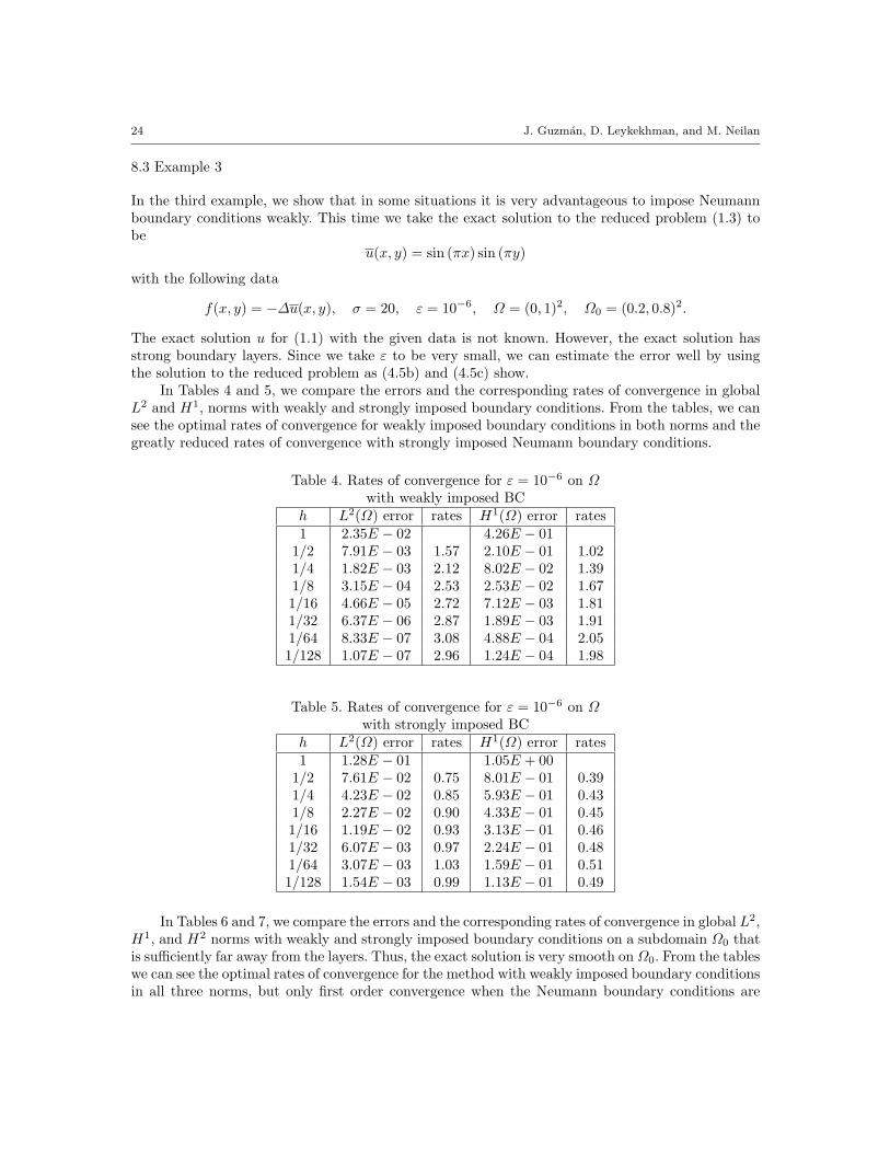
8.3 Example 3
In the third example, we show that in some situations it is very advantageous to impose Neumannboundary conditions weakly. This time we take the exact solution to the reduced problem (1.3) tobe
u(x, y) = sin (πx) sin (πy)
with the following data
f(x, y) = −∆u(x, y), σ = 20, ε = 10−6, Ω = (0, 1)2, Ω0 = (0.2, 0.8)2.
The exact solution u for (1.1) with the given data is not known. However, the exact solution hasstrong boundary layers. Since we take ε to be very small, we can estimate the error well by usingthe solution to the reduced problem as (4.5b) and (4.5c) show.
In Tables 4 and 5, we compare the errors and the corresponding rates of convergence in globalL2 and H1, norms with weakly and strongly imposed boundary conditions. From the tables, we cansee the optimal rates of convergence for weakly imposed boundary conditions in both norms and thegreatly reduced rates of convergence with strongly imposed Neumann boundary conditions.
Table 4. Rates of convergence for ε = 10−6 on Ωwith weakly imposed BC
h L2(Ω) error rates H1(Ω) error rates1 2.35E − 02 4.26E − 01
1/2 7.91E − 03 1.57 2.10E − 01 1.021/4 1.82E − 03 2.12 8.02E − 02 1.391/8 3.15E − 04 2.53 2.53E − 02 1.671/16 4.66E − 05 2.72 7.12E − 03 1.811/32 6.37E − 06 2.87 1.89E − 03 1.911/64 8.33E − 07 3.08 4.88E − 04 2.051/128 1.07E − 07 2.96 1.24E − 04 1.98
Table 5. Rates of convergence for ε = 10−6 on Ωwith strongly imposed BC
h L2(Ω) error rates H1(Ω) error rates1 1.28E − 01 1.05E + 00
1/2 7.61E − 02 0.75 8.01E − 01 0.391/4 4.23E − 02 0.85 5.93E − 01 0.431/8 2.27E − 02 0.90 4.33E − 01 0.451/16 1.19E − 02 0.93 3.13E − 01 0.461/32 6.07E − 03 0.97 2.24E − 01 0.481/64 3.07E − 03 1.03 1.59E − 01 0.511/128 1.54E − 03 0.99 1.13E − 01 0.49
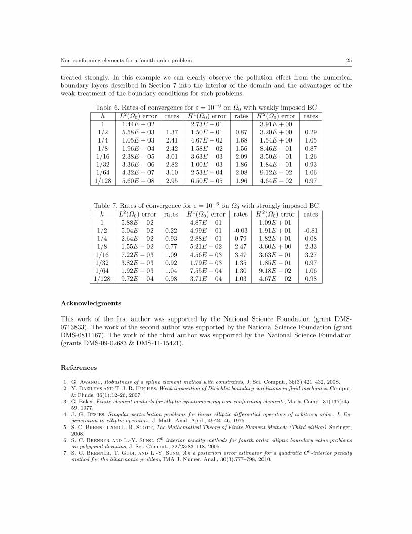
In Tables 6 and 7, we compare the errors and the corresponding rates of convergence in global L2,H1, and H2 norms with weakly and strongly imposed boundary conditions on a subdomain Ω0 thatis sufficiently far away from the layers. Thus, the exact solution is very smooth on Ω0. From the tableswe can see the optimal rates of convergence for the method with weakly imposed boundary conditionsin all three norms, but only first order convergence when the Neumann boundary conditions are
Non-conforming elements for a fourth order problem 25
treated strongly. In this example we can clearly observe the pollution effect from the numericalboundary layers described in Section 7 into the interior of the domain and the advantages of theweak treatment of the boundary conditions for such problems.
Table 6. Rates of convergence for ε = 10−6 on Ω0 with weakly imposed BCh L2(Ω0) error rates H1(Ω0) error rates H2(Ω0) error rates1 1.44E − 02 2.73E − 01 3.91E + 00
1/2 5.58E − 03 1.37 1.50E − 01 0.87 3.20E + 00 0.291/4 1.05E − 03 2.41 4.67E − 02 1.68 1.54E + 00 1.051/8 1.96E − 04 2.42 1.58E − 02 1.56 8.46E − 01 0.871/16 2.38E − 05 3.01 3.63E − 03 2.09 3.50E − 01 1.261/32 3.36E − 06 2.82 1.00E − 03 1.86 1.84E − 01 0.931/64 4.32E − 07 3.10 2.53E − 04 2.08 9.12E − 02 1.061/128 5.60E − 08 2.95 6.50E − 05 1.96 4.64E − 02 0.97
Table 7. Rates of convergence for ε = 10−6 on Ω0 with strongly imposed BCh L2(Ω0) error rates H1(Ω0) error rates H2(Ω0) error rates1 5.88E − 02 4.87E − 01 1.09E + 01
1/2 5.04E − 02 0.22 4.99E − 01 -0.03 1.91E + 01 -0.811/4 2.64E − 02 0.93 2.88E − 01 0.79 1.82E + 01 0.081/8 1.55E − 02 0.77 5.21E − 02 2.47 3.60E + 00 2.331/16 7.22E − 03 1.09 4.56E − 03 3.47 3.63E − 01 3.271/32 3.82E − 03 0.92 1.79E − 03 1.35 1.85E − 01 0.971/64 1.92E − 03 1.04 7.55E − 04 1.30 9.18E − 02 1.061/128 9.72E − 04 0.98 3.71E − 04 1.03 4.67E − 02 0.98
Acknowledgments
This work of the first author was supported by the National Science Foundation (grant DMS-0713833). The work of the second author was supported by the National Science Foundation (grantDMS-0811167). The work of the third author was supported by the National Science Foundation(grants DMS-09-02683 & DMS-11-15421).
References
1. G. Awanou, Robustness of a spline element method with constraints, J. Sci. Comput., 36(3):421–432, 2008.2. Y. Bazilevs and T. J. R. Hughes, Weak imposition of Dirichlet boundary conditions in fluid mechanics, Comput.
& Fluids, 36(1):12–26, 2007.3. G. Baker, Finite element methods for elliptic equations using non-conforming elements, Math. Comp., 31(137):45–
59, 1977.4. J. G. Besjes, Singular perturbation problems for linear elliptic differential operators of arbitrary order. I. De-
generation to elliptic operators, J. Math. Anal. Appl., 49:24–46, 1975.5. S. C. Brenner and L. R. Scott, The Mathematical Theory of Finite Element Methods (Third edition), Springer,
2008.6. S. C. Brenner and L.-Y. Sung, C0 interior penalty methods for fourth order elliptic boundary value problems
on polygonal domains, J. Sci. Comput., 22/23:83–118, 2005.7. S. C. Brenner, T. Gudi, and L.-Y. Sung, An a posteriori error estimator for a quadratic C0-interior penalty
method for the biharmonic problem, IMA J. Numer. Anal., 30(3):777–798, 2010.
26 J. Guzman, D. Leykekhman, and M. Neilan
8. S. C. Brenner and M. Neilan, C0 penalty methods for a fourth order elliptic singular perturbation problem,SIAM J. Numer. Anal., 49:869–892, 2011.
9. P. G. Ciarlet, The Finite Element Method for Elliptic Problems, North-Holland, Amsterdam, 1978.10. G. Engel, K. Garikipati, T. J. R. Hughes, M. G. Larson, L. Mazzei, and R. L. Taylor, Continu-
ous/discontinuous finite element approximations of fourth order elliptic problems in structural and continuummechanics with applications to thin beams and plates, and strain gradient elasticity, Comput. Meth. Appl. Mech.Eng., 191:3669–3750, 2002.
11. L. S. Frank, Singular Perturbations in Elasticity Theory, Analysis and its Applications, 1., IOS Press, Amster-dam, 1997.
12. P. Grisvard, Elliptic Problems on Nonsmooth Domains, Monographs and studies in mathematics, vol. 24, PitmanPublishing Inc., 1985.
13. P. Hansbo and M. Juntunen, Weakly imposed Dirichlet boundary conditions for the Brinkman model of porousmedia flow, Appl. Numer. Math., 59 (2009), pp. 1274–1289.
14. M. Juntunen, R. Stenberg, Analysis of finite element methods for the Brinkman problem, Calcolo, 47 (2010),pp. 129–147.
15. L. S. D. Morley, The triangular equilibrium element in the solution of plate bending problems, Aero. Quart.,19:149–169, 1968.
16. I. Mozolevski, E. Suli, P. R. Bosing, hp-version a priori error analysis of interior penalty discontinuousGalerkin finite element approximations to the biharmonic equation, J. Sci. Comput., 30 (2007), no. 3, 465-491.
17. T. K. Nilssen, X. C. Tai, and R. Winther, A robust nonconforming H2-element, Math. Comp., 70(234):489–505, 2001.
18. J. A. Nitsche, Uber ein Variationspirinzip zur Losung Dirichlet-Problemen bei Verwendung von Teilraumen,die keinen Randbedingungen unteworfen sind, Abh. Math. Sem. Univ. Hamburg, 36:9–15, 1971.
19. A. H. Schatz and L. B. Wahlbin, On the finite element method for singularly perturbed reaction-diffusionproblems in two and one dimensions, Math. Comp., 40:47–89, 1983.
20. F. Schieweck, On the role of boundary conditions for CIP stabilization of higher order finite elements, Electron.Trans. Numer. Anal., 32:1–16, 2008.
21. L. R. Scott and S. Zhang, Finite element interpolation of nonsmooth functions satisfying boundary conditions,Math. Comp., 54(190):483–493, 1990.
22. B. Semper, Conforming finite element approximations for a fourth-order singular perturbation problem, SIAMJ. Numer. Anal., 29(4):1043–1058, 1992.
23. B. Semper, Locking in finite-element approximations to long thin extensible beams, IMA J. Numer. Anal.,14(1):97–109, 1994.
24. Z. Shi, Error estimates of Morley element, Math. Numer. Sinica, 12(2):113–118, 1990.25. R. Stenberg, On some techniques for approximating boundary conditions in the finite element method, MJ.
Comput. Appl. Math. 63(1-3):139–148, 1995.26. X.-C. Tai and R. Winther, A discrete de Rham complex with enhanced smoothness, Calcolo, 43:287–306, 2006.27. M. Wang, The necessity and sufficiency of the patch test for the convergence of finite element methods, SIAM
J. Numer. Anal., 39(2):363–384, 2001.28. M. Wang, J. Xu, and Y-C. Hu, Modified Morley element method for a fourth order elliptic singular perturbation
problem, J. Comput. Math., 24(2):113–120, 2006.29. M. Wang and X. Meng, A robust finite element method for a 3-D elliptic singular perturbation problem, J.
Comput. Math., 25(6):631–644, 2007.30. P. Xie, D. Shi, and H. Li, A new robust C0-type nonconforming triangular element for singular perturbation
problems, Appl. Math. Comput., 217(8):3832–3843, 2010.


![Cours Elements Finis[1]](https://static.fdocument.org/doc/165x107/5571fa2449795991699162f9/cours-elements-finis1.jpg)