A EXPONENTIAL FAMILIES

This section reviews the standard results on exponentialfamilies in the literature [16, 2, 21]. A 1-dimensionalstandard exponential family [2, page 2] at its core canbe represented by a reference measure (R,B, ρp), wherethe set of outcomes (whether possible or not: see the def-inition of Ωp below) is given by R, the real numbers; theset of measurable sets is given by B, the Borel algebra ofR; and ρp : B → [0,∞] is a positive measure (often nota probability measure). Define Ap : R→ [−∞,+∞] tobe a normalization function where:

Ap(θ) = ln

(∫exp(θω)dρp(ω)

). (14)

If Ap is finite for all θ ∈ R, then p is defined to befull [2]. If p is full, then for each θ ∈ R, there is adistribution in the family of the form:

∀B ∈ B,Pr[x ∈ B|θ] =

∫B

exp(θω −Ap(θ))ρp(dω),

(15)

Full exponential families are also “regular” [2, page 2].Define Ωp to be the support of ρp, the minimal closed setW ⊆ R such that ρp(R−W) = 0, i.e. the possible out-comes. If p is full and |Ωp| > 1, it is “minimal” [2, page2].7 A full, minimal, 1-dimensional standard exponentialfamily p has a strictly convex Ap [2, Theorem 1.13] thatis infinitely differentiable everywhere [2, Theorem 2.2],

The likelihood of ω given θ is exp(θω−Ap(θ)). The neg-ative log likelihood of ω given θ is `p(ω, θ) = Ap(θ) −θω. Notice that if Ap is strictly convex, then `p is strictlyconvex in its second argument. The mean µp : R → Ris:

µp(θ) =

∫exp(θω −Ap(θ))ρp(dω). (16)

It is useful to define λp : R→ R to be:

λp(θ) =

∫exp(θω)ρp(dω). (17)

Now given these standard defintions, we canprove Lemma 1:

7The definition of minimal in [2, page 2] states that p is min-imal if the dimension of the convex hull of the support equalsthe dimension of the set of parameters where Ap is finite, butsince we are dealing with full, 1-dimensional, standard expo-nential families, that complexity is unnecessary, as the dimen-sion of the set of parameters where Ap is finite is always 1,and the dimension of the convex hull of the support is zero ifthe support has 1 point, and 1 if the support has two or morepoints.

Lemma 1 The Bernoulli family, Gaussian family (fixedvariance), and Poisson family are full, minimal, 1-dimensional standard exponential families. For a full,minimal, 1-dimensional standard exponential family p:

1. for every θ ∈ R, ω ∈ Ωp, `p(ω, θ) is differentiablewith respect to θ and ∂`p(ω,θ)

∂θ = µp(θ)− ω; and2. `p is strictly convex in its second argument: for

every θ, θ′ ∈ R, if θ 6= θ′, then for all λ ∈ (0, 1)we have `p(ω, λθ + (1− λ)θ′) < λ`p(ω, θ) + (1−λ)`p(ω, θ

′).

Proof: As we stated before, Ap is strictly convex if p isa full, minimal, 1 dimensional standard exponential fam-ily, and this implies that `p is strictly convex in its sec-ond argument. If p is a standard exponential family thatis full and minimal, then λp is infinitely differentiableeverywhere [2, Theorem 2.2], and by [2, page 34]:

λ′p(θ) =

∫ω exp(θω)ρp(dω) (18)

We then normalize:

λ′p(θ)

λp(θ)=

∫ω exp(θω)ρp(dω)

λp(θ)(19)

=

∫ω exp(θω)ρp(dω)

exp(Ap(θ))(20)

=

∫ω exp(θω −Ap(θ))ρp(dω) (21)

= µp(θ). (22)

So, for `p(ω, θ):

∂`p(ω, θ)

∂θ= A′p(θ)− ω (23)

=λ′p(θ)

λp(θ)− ω (24)

= µp(θ)− ω. (25)

Equation 25 is [16, Equation 3].

We now just have to show that |Ωp| > 1 and Ap is fi-nite everywhere for the families mentioned. It is naturalto think of the definition of ρp in terms of the possibleoutcomes, but Ωp is defined in terms of ρp. So, insteadwe define W as a set (that will turn out to be the possi-ble outcomes), define ρp in terms of W , and then showΩp = W . Note that if W is finite, to prove Ωp = W ,we need only prove that for all ω ∈ W , ρp(ω) > 0, andρp(R−W) = 0. IfW = R, then we need to show anyfinite, nonempty, open interval has positive measure toprove Ωp = W (this is because R − Ωp is open, and ifthere is some ω ∈ R − Ωp, then there must be a neigh-borhood N of ω (a finite, nonempty, open interval) inR− Ωp where ρp(N) = 0).

1. For the Bernoulli family of distributions, W =0, 1 and ρp(B) = |B ∩ W|. Thus, ρp(0) =ρp(1) = 1, and ρp(R−W) = |(R−W)∩W| =0, so Ωp = W . Also, Ap(θ) = − ln(1 + exp(θ)),Pr[ω|θ] = exp(θω)

1+exp(θ) , and `p(ω, θ) = −θω + ln(1 +

exp(θ)), and µp(θ) = 11+exp(−θ) . Since Ap(θ) is

finite everywhere, the Bernoulli family is full, andsince |Ωp| > 1, the Bernoulli family is minimal.

2. For the Gaussian family of distributions with fixedmean σ2 = 1 we have W = R, but we also needto define a particular ρp. Specifically, define someh(ω) = 1√

2πexp(−ω

2

2 ). For any Borel measurableset, define ρp(B) =

∫Bh(ω)dω, where the right

hand side is the standard Lebesgue integral. Noteρp itself is a Gaussian with mean zero and vari-ance one. Since h(ω) > 0 and h(ω) is continu-ous, on any finite, closed interval [a, b] it has a mini-mum m > 0, and therefore on any finite, nonempty,open interval (a, b), ρp((a, b)) ≥ (b − a)m, soΩp = W . Thus, Ap(θ) = θ2

2 , Pr[ω ∈ B|θ] =1√2π

∫B

exp(− (ω−θ)2

2

)dω, µp(θ) = θ, the likeli-

hood8 is exp(θω − θ2

2 ), and `p(θ, ω) = θ2

2 − θω =12 (θ − ω)2 + ω2

2 . Notice that this loss is off by ω2

2from squared loss, and this term is independent of θ.Finally, |Ωp| > 1,Ap is finite everywhere, implyingp is a full, minimal, standard, 1-dimensional family.

3. For the Poisson family of distributions W =0, 1, 2 . . .. Define ρp(B) =

∑ω∈W∩B

1ω! , so

Ap(θ) = exp(θ). Moreover, for any non-negativeinteger ω, ρp(ω) = 1

ω! , and ρp(R − W) is thesum over an empty set, and therefore zero. Finally,Pr[ω|θ] = 1

ω! exp(θω − exp(θ)), and the likeli-hood9 is exp(θω − exp(θ)). µp(θ) = exp(θ) and`p(ω, θ) = exp(θ) − θω. Again, |Ωp| > 1, and Apis finite everywhere.

B RELATION TO TRADITIONALLAYERED NEURAL NETWORKS

A more conventional way to represent a network involveswriting layers, by interleaving fixed activation functionswith learned affine functions. We imagine a sequence ofintegers n0 . . . nk, representing the number of nodes in

8Note the distinction here between the conventional densitydefined with respect to the Lebesgue measure, and this likeli-hood defined with respect to ρ. However, since we are tuning θand ω is given, this is simply a constant in `p.

9As before, there is a slight distinction between the conven-tional probability mass and the likelihood as defined here.

each layer, with 0 being the input layer (with X = Rn0 ),and k being the output layer (with nk = 1). We choosean activation function ai : R → R for each layer0, . . . k − 1, and define Ai : Rni → Rni such that(Ai(v))j = ai(vj) for all v ∈ Rni , for all j ∈ 1 . . . ni.Often a0 is the identity, and a1 . . . ak−1 are relu, sig-moid, or some other standard function.

Then, in-between these layers, we have a matrix W i ∈Rni×ni−1 and a vector wi ∈ Rni . We define h0 :Rn0 → Rn0 to be the identity. We can then definehi : Rn0 → Rni for i ∈ 1 . . . k recursively such thathi(x) = W iAi−1(hi−1(x)) + wi). The model in thisform is MW,w(x) = hk(x)1. As we will show, these canbe easily modeled in our graph representation. However,we will see that learning affine (as opposed to linear)functions show that the conventional concept of “layer”is not as crisp and neat as one would like.

B.1 REPRESENTATION AS A GRAPH

First of all, this kind of model can be represented in thegraph network that we describe in Section 5. Most oddi-ties of the representation come from the bias features.

1. For each i ∈ 1 . . . k, define Vi = vi,1 . . . vi,ni,and let vc be a special vertex (which will be a specialinput node that will always equal 1).

2. Define V = vc ∪⋃ki=0 Vi.

3. Define I = V0 ∪ vc.4. Define o∗ = vk,1,5. For i ∈ 0, . . . k − 1, for all j ∈ 1 . . . ni, letavi,j = ai.

6. Define ao∗ and avc to be the identity.7. For all x ∈ X , for all j ∈ 1 . . . n0, let gv0,j (x) =xj .

8. For all x ∈ X , gvc(x) = 1.9. The edges associated with W i are Ei = Vi−1 × Vi.

10. The edges associated with wi are Eci = vc × Vi.11. Define E =

⋃ki=1Ei ∪ Eci .

D=(V,E, I, gii∈I , o∗, avv∈V ) is a neural network,equivalent to the layered form we described in the previ-ous section.

In the next section, we will show how the edges in Eci(associated with the bias parameters) play an unusualrole in our work.

B.2 AN ORDERED CUT IN A LAYEREDNEURAL NETWORK

We introduced ordered cuts and cut sets in Section 6. Themost obvious cut would be Bi = vc ∪

⋃i−1j=0 Vj and

TB

vc v0,1 v0,2 v0,3

v1,3v1,2v1,1

v2,1 v2,2 v2,3

v3,3v3,2v3,1

v4,1 v4,2 v4,3

v5,1

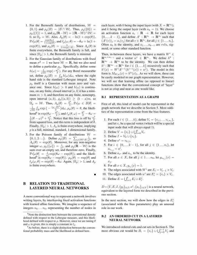
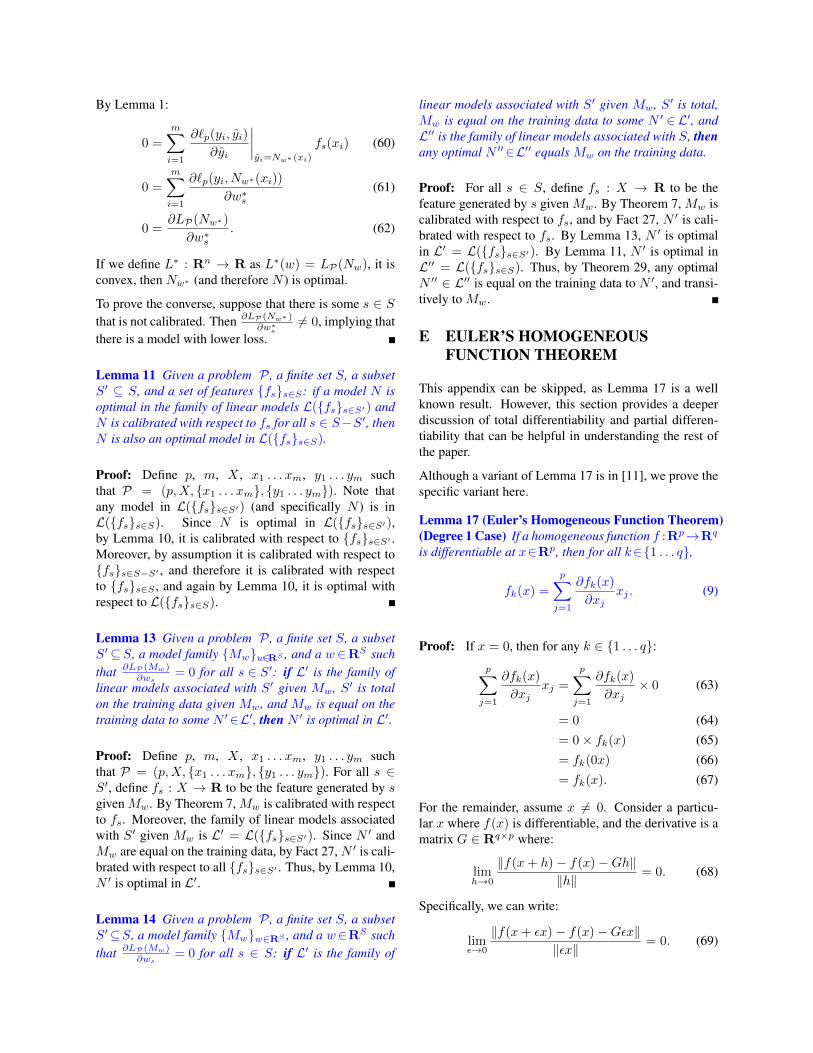
Figure 5: A traditional neural network represented as agraph, with 4 fully connected hidden layers, and a biasparameter for each node. The input nodes are squares,and the internal nodes are circles, with the output nodeon top. The ordered cut is indicated with the white nodesand the black nodes, and the edges in the cut set are red.Note that while this ordered cut naturally separates thesecond and third hidden layers, bias parameters from thethird, fourth, and fifth layer are in the cut set.

Ti =⋃kj=i Vj , and these are the ones we use in the ex-

periments.

Suppose k = 5, and we consider the cut B2, T2, thenthe cut set E′ is the set of edges with one endpoint in B2

and one endpoint in T2 (see Figure 5). Obviously, E2 isa subset of the cut set, as is Ec2. Less obviously, Ec3, Ec4,and Ec5 are also subsets of the cut set.10 However, uponreflection this makes sense: the proof in Appendix F re-lies on the network after the cut set to be a homogeneousfunction, and affine functions with nonzero offsets arecertainly not homogeneous functions.

This is the reason that we use the graph representation tointroduce our results. Cut sets have very counterintuitiveproperties in the conventional representation, but oncethe traditional representations are reduced to a network,they make perfect sense.

10Keep in mind, while Ec5 is in the cut set, it only contains

one parameter, and the generated (holographic) feature is al-ways 1.

B.3 EXPLORING THE NATURE OFGENERATED FEATURES

So, as we consider these conventional networks, it is nat-ural to ask, what does a generated feature look like? Howdoes it relate to a conventional activation feature? Let usbreak this down into features generated from weight ma-tricesW (orE1 . . . Ek), and features generated from biasvectors w (or Ec1 . . . E

ck). In this section, for simplicity

we assume that partial derivatives exist where necessary:see Appendix I for a deeper discussion of differentiabil-ity in deep networks.

We consider the bias features first for some layer i ∈1 . . . k − 1. For any j ≥ i, we can recursively definehj,i : Rni → Rnj such that hi,i(v) = v and for allj ∈ i + 1 . . . k, hj,i(v) = W jAj−1(hj−1,i(v)) + wj .This is an accumulation of the transforms after the inputof layer i, and for all x ∈ X:

MW,w(x) = hk,i(hi(x)) (26)

MW,w(x) = hk,i(W iAi−1(hi−1(x)) + wi). (27)

For some q ∈ 1 . . . ni, if we define f iq : X → R to bethe feature generated from (vc, vi,q), then we can write:

f iq(x) =∂MW,w(x)

∂wiq(28)

=∂hk,i(v)

∂vq

∣∣∣∣v=W iAi−1(hi−1(x))+wi

. (29)

Notice that this is the partial derivative of the predictionwith respect to the input of node vi,q .

Next, we consider features generated from a weightmatrix. Consider some i ∈ 1 . . . k, some p ∈1 . . . ni−1 and some q ∈ 1 . . . ni. Then(vi−1,p, vi,q) ∈ Ei is the edge related to parameterW i

q,p.Define F iq,p : X → R to be the feature generated from(vi−1,p, vi,q). Using hk,i again:

F iq,p(x) =∂MW,w(x)

∂W iq,p

(30)

=∂hk,i(v)

∂vq

∣∣∣∣v=W iAi−1(hi−1(x))+wi

Ai−1p (hi−1(x))

(31)

= f iq(x)ai−1(hi−1p (x)). (32)

So, the generated feature from (vi−1,p, vi,q) is the acti-vation feature of vi−1,p times the generated feature of(vc, vi,q).

In summary, the generated features of conventional lay-ers have a nice form, and one can take a conventionallayered network and translate it into a graph. However,

from a mathematical perspective, it is much easier to rea-son about graphs, because of the clean concept of cutsand cut sets. Moreover, the bias features work in highlycounterintuitive ways, and presenting a theory withoutthem tells an incomplete story.

C CONVEXITY

In this section, we will state some known results aboutconvexity.

Fact 27 Given a supervised learning problem P =(p,X, x1 . . . xm, y1 . . . ym), given two models M :X → R andM ′ : X → R that are equal on the trainingdata, if M is calibrated on a feature f : X → R, thenM ′ is calibrated on f .

One can think about the model as mapping a matrix ofinputs to a vector of predictions, which is then composedwith a loss function that maps a vector of predictions toa single loss. Next, we show when this second mappingwill be (strictly) convex.

Lemma 28 Given convex sets C1 . . . Cm ⊆ R, for eachi ∈ 1 . . .m a function Li : Ci → R, then if C =×mi=1Ci, and there is a function L : C → R such thatfor all x ∈ C:

L(x) =

m∑i=1

Li(xi), (33)

then:

1. if for all i, Li is convex, then L is convex.2. if for all i, Li is strictly convex, then L is strictly

convex.

Proof: Consider x, y ∈ C, and λ ∈ [0, 1]. Withoutloss of generality, assume x 6= y, and λ ∈ (0, 1). Byconvexity, for all i, λLi(xi)+(1−λ)Li(yi) ≥ Li(λxi+(1− λ)yi), so:

L(λx+ (1− λ)y)

=

m∑i=1

Li(λxi + (1− λ)yi) (34)

≤m∑i=1

(λLi(xi) + (1− λ)L(yi)) (35)

≤ λm∑i=1

Li(xi) + (1− λ)

m∑i=1

L(yi) (36)

≤ λL(x) + (1− λ)L(y). (37)

To prove the result for strong convexity, we need to bea little more careful. Since x 6= y, there exists a j ∈

1 . . .m where xj 6= yj . So Lj(λxj + (1 − λ)yj) <λLj(xj) + (1− λ)Lj(yj). Thus:

L(λx+ (1− λ)y)

= Lj(λxj + (1− λ)yj)

+∑i 6=j

Li(λxi + (1− λ)yi) (38)

< λLj(xj) + (1− λ)Lj(yj)

+∑i 6=j

Li(λxi + (1− λ)yi) (39)

< λLj(xj) + (1− λ)Lj(yj)

+∑i 6=j

(λLi(xi) + (1− λ)Li(yi)) (40)

<m∑i=1

(λLi(xi) + (1− λ)Li(yi)) (41)

< λ

m∑i=1

Li(xi) + (1− λ)

m∑i=1

Li(yi) (42)

< λL(x) + (1− λ)L(y). (43)

D PROOFS OF CALIBRATION ONGENERATED FEATURES

Next we show that if the partial derivative of the loss withrespect to a parameter is zero, then the feature generatedby that parameter is calibrated.

Theorem 7 For a problem P and model family M =Mww∈RS , given a w ∈ RS and s ∈ S such thatfs is the feature generated from parameter s of modelMw: if s is total on the training data given Mw and∂LP(Mw)

∂ws= 0, then Mw is calibrated with respect to fs.

Proof: Define p, m, X , x1 . . . xm, y1 . . . ym suchthat P = (p,X, x1 . . . xm, y1 . . . ym). We be-gin with the partial derivative of LP . Note thatfrom Lemma 1, `p is partially differentiable with respectto its second argument, and since for any i ∈ 1 . . .ms is total for xi given Mw, then Mw(xi) is partially

differentiable with respect to ws. Therefore:

0 =∂LP(Mw)

∂ws(44)

=∂

∂ws

m∑i=1

`p(yi,Mw(xi)) (45)

=

m∑i=1

∂`p(yi,Mw(xi))

∂ws(46)

=

m∑i=1

∂`p(yi, yi)

∂yi

∣∣∣∣yi=Mw(xi)

∂Mw(xi)

∂ws(47)

=

m∑i=1

(µp(Mw(xi))− yi)∂Mw(xi)

∂ws. (48)

The last step is because of Lemma 1. For any i ∈1 . . .m, since Mw(xi) is partially differentiable withrespect to ws, we can use fs(xi) = ∂+Mw(xi)

∂ws=

∂Mw(xi)∂ws

to get:

0 =

m∑i=1

(µp(Mw(xi))− yi)fs(xi) (49)

m∑i=1

yifs(xi) =

m∑i=1

µp(Mw(xi))fs(xi). (50)

Lemma 9 For finite S, given a set of features fss∈S ,the family of linear models L(fss∈S), and Nw ∈ L:the set S is total for all x ∈ X given Nw, and the featuregenerated from parameter s by model Nw is fs.

Proof: First note that, by definition, a linear model is alinear function of w, and therefore a differentiable func-tion of w regardless of the input or w. Thus, for anyx ∈ X , for any w, the set S is total. Notice that, for anyx ∈ X:

∂Mw(x)

∂ws=

∂

∂ws

∑t∈S

wtft(x) (51)

=∑t∈S

∂

∂ws(wtft(x)) (52)

= fs(x). (53)

Another known key result about linear models is that anytwo linear models that minimize loss will produce thesame predictions on the training data.

Theorem 29 Given a supervised learning problemP = (p,X, x1 . . . xm, y1 . . . ym), a set of features

f1 . . . fn : X → R, and a family of linear modelsL(f1 . . . fn), if two models M,M ′ ∈ L are optimalin L for P , then they are equal on the training data.

Proof: Define L∗ : Rm → R such that for all y ∈ Rm:

L∗(y) =

m∑i=1

`p(yi, yi). (54)

By Lemma 1, each `p is strictly convex in its secondargument. By Lemma 28,11 L∗ is strictly convex. Wedefine P : Rn → Rm, such that for all v ∈ Rn,for all i ∈ 1 . . .m, Pi(v) = Mv(xi). Therefore,L∗(P (v)) = LP(Mv). We need to prove P (w) =P (w′).

Consider w′′ = w+w′

2 . Since the models are linear, weknow that for all x ∈ X , Mw′′(x) = Mw(x)+Mw′ (x)

2 .

Thus, P (w′′) = P (w)+P (w′)2 . Assume for the sake of

contradiction, P (w) 6= P (w′). Since L∗ is strictly con-vex:

L∗(P (w′′)) <L∗(P (w)) + L∗(P (w′))

2; (55)

since L∗(P (v)) = LP(Mv):

LP(Mw′′) <LP(Mw) + LP(Mw′)

2; (56)

since LP(Mw) = LP(Mw′):

LP(Mw′′) < LP(Mw). (57)

This contradicts the original hypothesis that both areminima. Thus, P (w) = P (w′), which is the same assaying, for all i ∈ 1 . . .m, Mw(xi) = Mw′(xi).

Lemma 10 (c.f. [16, Equation 10]) Given a problem P ,a finite set S and a set of features fss∈S: a modelN inthe family of linear models L(fss∈S) is optimal if andonly if N is calibrated with respect to fs for all s ∈ S.

Proof: Define p, m, X , x1 . . . xm, y1 . . . ym suchthat P = (p,X, x1 . . . xm, y1 . . . ym). DefineNww∈RS = L(fss∈S) where Nw(x) =∑s∈S wsfs(x). Define w∗ ∈ RS such that Nw∗ = N .

If N (and therefore Nw∗ ) is calibrated, for all s ∈ S:m∑i=1

µp(Nw∗(xi))fs(xi) =

m∑i=1

yifs(xi) (58)

0 =

m∑i=1

(yi − µp(Nw∗(xi)))fs(xi).

(59)

11Formally, for all i ∈ 1 . . .m, we could define Li : R →R such that Li(yi) = `p(yi, yi).

By Lemma 1:

0 =

m∑i=1

∂`p(yi, yi)

∂yi

∣∣∣∣yi=Nw∗ (xi)

fs(xi) (60)

0 =

m∑i=1

∂`p(yi, Nw∗(xi))

∂w∗s(61)

0 =∂LP(Nw∗)

∂w∗s. (62)

If we define L∗ : Rn → R as L∗(w) = LP(Nw), it isconvex, then Nw∗ (and therefore N ) is optimal.

To prove the converse, suppose that there is some s ∈ Sthat is not calibrated. Then ∂LP(Nw∗ )

∂w∗s6= 0, implying that

there is a model with lower loss.

Lemma 11 Given a problem P , a finite set S, a subsetS′ ⊆ S, and a set of features fss∈S: if a model N isoptimal in the family of linear models L(fss∈S′) andN is calibrated with respect to fs for all s ∈ S−S′, thenN is also an optimal model in L(fss∈S).

Proof: Define p, m, X , x1 . . . xm, y1 . . . ym suchthat P = (p,X, x1 . . . xm, y1 . . . ym). Note thatany model in L(fss∈S′) (and specifically N ) is inL(fss∈S). Since N is optimal in L(fss∈S′),by Lemma 10, it is calibrated with respect to fss∈S′ .Moreover, by assumption it is calibrated with respect tofss∈S−S′ , and therefore it is calibrated with respectto fss∈S , and again by Lemma 10, it is optimal withrespect to L(fss∈S).

Lemma 13 Given a problem P , a finite set S, a subsetS′⊆S, a model family Mww∈RS , and a w∈RS suchthat ∂LP(Mw)

∂ws= 0 for all s ∈ S′: if L′ is the family of

linear models associated with S′ given Mw, S′ is totalon the training data given Mw, and Mw is equal on thetraining data to some N ′∈L′, then N ′ is optimal in L′.

Proof: Define p, m, X , x1 . . . xm, y1 . . . ym suchthat P = (p,X, x1 . . . xm, y1 . . . ym). For all s ∈S′, define fs : X → R to be the feature generated by sgiven Mw. By Theorem 7, Mw is calibrated with respectto fs. Moreover, the family of linear models associatedwith S′ given Mw is L′ = L(fss∈S′). Since N ′ andMw are equal on the training data, by Fact 27, N ′ is cali-brated with respect to all fss∈S′ . Thus, by Lemma 10,N ′ is optimal in L′.

Lemma 14 Given a problem P , a finite set S, a subsetS′⊆S, a model family Mww∈RS , and a w∈RS suchthat ∂LP(Mw)

∂ws= 0 for all s ∈ S: if L′ is the family of

linear models associated with S′ given Mw, S′ is total,Mw is equal on the training data to some N ′ ∈ L′, andL′′ is the family of linear models associated with S, thenany optimal N ′′∈L′′ equals Mw on the training data.

Proof: For all s ∈ S, define fs : X → R to be thefeature generated by s given Mw. By Theorem 7, Mw iscalibrated with respect to fs, and by Fact 27, N ′ is cali-brated with respect to fs. By Lemma 13, N ′ is optimalin L′ = L(fss∈S′). By Lemma 11, N ′ is optimal inL′′ = L(fss∈S). Thus, by Theorem 29, any optimalN ′′ ∈ L′′ is equal on the training data to N ′, and transi-tively to Mw.

E EULER’S HOMOGENEOUSFUNCTION THEOREM

This appendix can be skipped, as Lemma 17 is a wellknown result. However, this section provides a deeperdiscussion of total differentiability and partial differen-tiability that can be helpful in understanding the rest ofthe paper.

Although a variant of Lemma 17 is in [11], we prove thespecific variant here.

Lemma 17 (Euler’s Homogeneous Function Theorem)(Degree 1 Case) If a homogeneous function f :Rp→Rq

is differentiable at x∈Rp, then for all k∈1 . . . q,

fk(x) =

p∑j=1

∂fk(x)

∂xjxj . (9)

Proof: If x = 0, then for any k ∈ 1 . . . q:p∑j=1

∂fk(x)

∂xjxj =

p∑j=1

∂fk(x)

∂xj× 0 (63)

= 0 (64)= 0× fk(x) (65)= fk(0x) (66)= fk(x). (67)

For the remainder, assume x 6= 0. Consider a particu-lar x where f(x) is differentiable, and the derivative is amatrix G ∈ Rq×p where:

limh→0

‖f(x+ h)− f(x)−Gh‖‖h‖

= 0. (68)

Specifically, we can write:

limε→0

‖f(x+ εx)− f(x)−Gεx‖‖εx‖

= 0. (69)

In the limit, ε > −1, so by the homogeneous property:

limε→0

‖(1 + ε)f(x)− f(x)−Gεx‖‖εx‖

= 0 (70)

limε→0

‖εf(x)−Gεx‖ε ‖x‖

= 0 (71)

limε→0

‖f(x)−Gx‖‖x‖

= 0 (72)

‖f(x)−Gx‖‖x‖

= 0 (73)

‖f(x)−Gx‖ = 0 (74)f(x) = Gx. (75)

Since Gk,j = ∂fk(x)∂xj

, the result follows.

One might wonder, is it possible to prove this for func-tions that are only partially (and not totally) differen-tiable? Yes and no: for one or two dimensions partiallydifferentiability is sufficient for Euler’s function to hold,but for three or more dimensions, there is no such guaran-tee, and we can demonstrate this with a counterexample.

Lemma 30 If a homogeneous function f : Rp → Rq ispartially differentiable at a point x ∈ Rp, and p ≤ 2,then for all k ∈ 1 . . . q:

fk(x) =

p∑j=1

∂fk(x)

∂xjxj . (76)

Proof: Since partial differentiability implies differen-tiability when p = 1, the proof for p = 1 follows di-rectly from Lemma 17. So, we assume p = 2. Considera specific point (x, y) where f is partially differentiable,i.e. ∂f(x,y)∂x and ∂f(x,y)

∂y exist. If x = 0 or y = 0, thenit is basically analogous to the one dimensional case, asthe function along the axis can be considered a 1 dimen-sional homogeneous function that is differentiable at thatpoint.

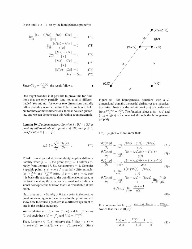
Next, assume x > 0 and y > 0, i.e. a point in the positivequadrant as in Figure 6: near the end of the proof, we willshow how to reduce a problem in a different quadrant toone in the positive quadrant.

We can define g : (0, x) → (0,∞) and h : (0, x) →(0,∞) such that g(ε) = yε

x−ε and h(ε) = y+g(ε)y .

Then, for any ε ∈ (0, x), observe that h(ε)(x − ε, y) =(x, y+g(ε)), so h(ε)f(x− ε, y) = f(x, y+g(ε)). Since

(x,y)(x-𝜖,y)

(x,y+g(𝜖))

a

𝜖

g(𝜖)b

x

y

(0,0) (x,0)

Figure 6: For homogeneous functions with a 2-dimensional domain, the partial derivatives are inextrica-bly linked. Note that the definition of g(ε) can be derivedfrom g(ε)+y

x = g(ε)ε . The function values at (x−ε, y) and

(x, y + g(ε)) are connected through the homogeneousproperty.

limε→0+ g(ε) = 0, we know that:

∂f(x, y)

∂y= limε→0+

f(x, y + g(ε))− f(x, y)

g(ε)(77)

∂f(x, y)

∂y= limε→0+

f(x− ε, y)h(ε)− f(x, y)

g(ε)(78)

∂f(x, y)

∂y= limε→0+

f(x− ε, y)h(ε)− f(x, y)h(ε)

g(ε)

+ limε→0+

f(x, y)h(ε)− f(x, y)

g(ε)

(79)

∂f(x, y)

∂y= limε→0+

f(x− ε, y)− f(x, y)

εlimε→0+

h(ε)ε

g(ε)

+ f(x, y) limε→0+

h(ε)− 1

g(ε).

(80)

First, observe that limε→0+f(x−ε,y)−f(x,y)

ε = −∂f(x,y)∂x .Notice that for ε ∈ (0, x):

h(ε)− 1

g(ε)=

y+g(ε)y − 1

g(ε)=

1

y. (81)

Also, since limε→0+ h(ε) = 1, for ε ∈ (0, x):

limε→0+

h(ε)ε

g(ε)= limε→0+

ε

g(ε)(82)

= limε→0+

ε(x− ε)yε

(83)

=x

y. (84)

So, from Equation 80:

∂f(x, y)

∂y= −∂f(x, y)

∂x

x

y+ f(x, y)

1

y(85)

∂f(x, y)

∂xx+

∂f(x, y)

∂yy = f(x, y), (86)

which is Euler’s function.

Now if x < 0 or y < 0, we could flip the functionon one axis or on both without affecting homogene-ity, partial differentiability, or Euler’s function. Specif-ically, note that if we defined f∗ : R2 → R suchthat for all x′, y′ ∈ R, f∗(x′, y′) = f(−x′, y′), then∂f∗(−x,y)

∂x = −∂f(x,y)∂x , ∂f∗(−x,y)∂y = ∂f∗(−x,y)

∂y , and if

f∗(−x, y) = ∂f∗(−x,y)∂x (−x) + ∂f∗(−x,y)

∂x y then:

f(x, y) = f∗(−x, y) (87)

=∂f∗(−x, y)

∂x(−x) +

∂f∗(−x, y)

∂xy (88)

= (−∂f(−x, y)

∂x)(−x) +

∂f(−x, y)

∂xy (89)

=∂f(−x, y)

∂xx+

∂f(−x, y)

∂xy. (90)

Similarly for flipping on the x axis.

However, if we add a third dimension, things get incred-ibly complex. Consider the following function:

f(x, y, z) =

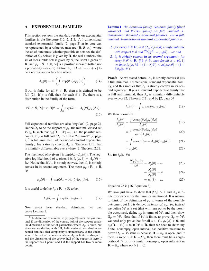
7z − x if x+ y − 2z ≥ 0 and x− y < 07z − y if x− y ≥ 0 and x+ y − 2z > 0x+ 5z if x+ y − 2z ≤ 0 and x− z > 07z − x if x− z ≤ 0 and x− y > 07z − y if x− y ≤ 0 and y − z < 0y + 5z if y − z ≥ 0 and x+ y − 2z < 0y + 5z if x = y = z

(91)

So, we wish to establish five things:

1. f is well-defined.2. f is continuous.3. f is homogeneous.4. f has partial derivatives at (1, 1, 1).

x-y=0 x-z=0

y-z=0

x+y-2z=0

f(x,y,z)=y+5z

f(x,y,z)=7z-x

f(x,y,z)=7z-yf(x,y,z)=7z-y

f(x,y,z)=7z-x f(x,y,z)=x+5z

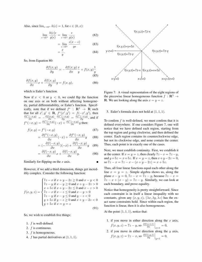
Figure 7: A visual representation of the eight regions ofthe piecewise linear homogeneous function f : R3 →R. We are looking along the axis x = y = z.

5. Euler’s formula does not hold at (1, 1, 1).

To confirm f is well-defined, we must confirm that it isdefined everywhere. If one considers Figure 7, one willnotice that we have defined each region, starting fromthe top region and going clockwise, and then defined thecenter. Each region contains its counterclockwise edge,but not its clockwise edge, and none contain the center.Thus, each point is in exactly one of the cases.

Next, we must establish continuity. First, we establish itat the center. If x = y = z, then clearly 7z−x = 7z−y,and y+5z = x+5z. If x = y = z, then x+y−2z = 0,so 7z − x = 7z − x− (x+ y − 2z) = x+ 5z.

Thus, all four linear functions equal each other along theline x = y = z. Simple algebra shows us, along theplane x − y = 0, 7z − x = 7z − y, because 7z − x =7z − x + (x − y) = 7z − y. Similarly, we can look ateach boundary, and prove equality.

Notice that homogeneity is pretty straightforward. Sinceeach constraint is in itself a linear inequality with noconstants, given any (x, y, z), (λx, λy, λz) has the ex-act same constraints hold. Since within each region, thefunction is linear, then it is also homogeneous.

At the point (1, 1, 1), notice that:

1. if you move in either direction along the x axis,f(x, y, z) = 7z − y, so ∂f(x,1,1)

∂x

∣∣∣x=1

= 0,

2. if you move in either direction along the y axis,f(x, y, z) = 7z − x, so ∂f(1,y,1)

∂y

∣∣∣y=1

= 0,

3. and if you move in either direction along the z axis,you will stay where x − y = 0, so f(x, y, z) =

7z − x, so ∂f(1,1,z)∂z

∣∣∣z=1

= 7.

Note that f(1, 1, 1) = 6. However:

∂f(x, 1, 1)

∂x

∣∣∣∣x=1

×1+∂f(1, y, 1)

∂y

∣∣∣∣y=1

×1+∂f(1, 1, z)

∂z

∣∣∣∣z=1

×1

= 0× 1 + 0× 1 + 7× 1 = 7. (92)

Thus, since 6 6= 7 , this function, while homogeneousand continuous, has a point where it is partially differen-tiable, but Euler’s formula does not hold.

With further effort, we can also show that the functioncan be constructed using relu gates. Thus, in a very cru-cial way, Euler’s function requires total differentiability,justifying the large role this concept of total features hasin our theoretical analysis. However, as our empiricalanalysis shows, we can pretty much ignore this concernin practice. In Appendix I, we give a sufficient condition(based on a complex proof) to determine if the model istotal on an input.

F PROOFS FOR HOMOGENEOUSFUNCTIONS

Before continuing, it is important to note that when defin-ing the homogeneous property of a model family, we di-rectly appealed to a property of differentiability due tothe technical issues described in higher dimensional ho-mogeneous functions in Appendix E.

We now prove Theorem 20:

Theorem 20 If a model family M is homogeneous onthe parameter set S′, M ∈ M, L′ is the family of linearmodels associated with S′ given M , and S′ is total onthe training data givenM , then there existsN ∈ L′ suchthat M and N are equivalent on the training data.

Proof: Define M = M ′ww∈RS , and w ∈ RS suchthat M ′w = M . Given some x in the training data, sinceM is homogeneous with respect to S′, and S′ is total onx given M ′w, then by Lemma 17:

M ′w(x) =∑s∈S′

∂M ′w(x)

∂wsws. (93)

Since fs(x) =∂+M ′w(x)∂ws

is the feature generated by sgiven M , if x is in the training data, thens ⊆ S′ istotal on x given M ′w, and fs(x) =

∂M ′w(x)∂ws

, so:

M ′w(x) =∑s∈S′

wsfs(x). (94)

Note L′ = L(fss∈S′), and if N ′ww∈RS′ = L′, thenfor the w′ ∈ RS′ where w′s = ws for all s ∈ S′:

N ′w′(x) =∑s∈S′

w′sfs(x) (95)

=∑s∈S′

wsfs(x) (96)

= M ′w(x) = M(x), (97)

so M(x) = N ′w′(x) on the training data, and N ′w′ is inthe family of linear models associated with S′ given M .

We now prove Theorem 23:

Theorem 23 Given a problem P and a family of feed-forward network models D(V,E, I, gii∈I , o∗, A) =Mww∈RE , where all a ∈ A are homogeneous: if Band T is an ordered cut of the feedforward network, suchthat E′ is the cut set, then:

1. Mww∈RE is homogeneous on E′;2. for some w ∈ RE , if E′ is total on the training

data given Mw, L′ is the family of linear modelsassociated with E′ given Mw, and ∂LP(Mw)

∂we= 0

for all e ∈ E′, then Mw is equal on the trainingdata to any optimal model in L′;

3. for some w ∈ RE , if L′ is the family of linear mod-els associated with E given Mw, if E is total on thetraining data given Mw, and ∂LP(Mw)

∂we= 0 for all

e ∈ E, thenMw is equal on the training data to anyoptimal model in L′.

Proof: We need only prove that the model family ishomogeneous: the other two results follow from Theo-rem 20, Lemma 13, and Lemma 14. We need to con-struct a function from the inputs passing through thecut set to the second part of the function. First, defineE′′ = E −E′, and given w, define w′′ ∈ RE′′ such thatfor all e ∈ E′′, w′′e = we. Thus, for all t ∈ T , definedt,w′′ : RE′ → R recursively (using the partial orderingof the vertices in the network) such that for all z ∈ RE′ :

dt,w′′(z) = at

( ∑u:(u,t)∈E′

z(u,t)

+∑

u:(u,t)∈E′′du,w′′(z)w

′′(u,t)

). (98)

We subscript this by w′′ to indicate that dt,w′′ is inde-pendent of the weights in E′. An important point to noteis that for any x ∈ X , for any b ∈ B, cb,w(x) doesnot depend upon the weight of any edge in E′. For any

(b, t) ∈ E′, we can write gw′′(x)(b,t) = cb,w(x) to for-malize this idea. Define w′ ∈ RE′ such that for all e ∈RE′ , w′e = we. Finally, for any z, z′ ∈ RE′ we denotethe Hadamard (entrywise) product as (z z′)e = zez

′e.

We can prove recursively, for all t ∈ T :

ct,w(x) = dt,w′′(w′ gw′′(x)). (99)

Importantly, this means:

Mw(x) = co∗,w(x) (100)= dt,w′′(w

′ gw′′(x)). (101)

We can use this formulation to prove Mw(x) is homoge-neous inw′. First, we can prove recursively that dt,w′′(z)is a homogeneous function of z: since all a ∈ A are ho-mogeneous, it is a homogeneous function of the sum of aset of projections (and all projections are homogeneous)and a set of homogeneous functions multiplied by a con-stant. To prove that the overall function is homogeneous,we introduce λ ≥ 0, v ∈ RE , v′ ∈ RE′ , and v′′ ∈ RE′′ ,such that v′s = vs for all s ∈ E′, v′′s = vs for all s ∈ E′′,v′′ = w′′, and v′ = λw′. Note that:

Mv(x) = co∗,v(x) (102)= dt,v′′(v

′ gv′′(x)) (103)= dt,w′′((λw

′) gw′′(x)) (104)= dt,w′′(λ(w′ gw′′(x))). (105)

Since dt,w′′ is homogeneous:

Mv(x) = λdt,w′′(w′ gw′′(x)) (106)

= λMw(x). (107)

We have established that Mw(x) is homogeneous withrespect to w′. Thus, from Theorem 20, Lemma 13, andLemma 14, the other results hold.

G PROOFS FOR RESNETS AND CNNS

Recall the main theorem about ResNets and CNNs:

Theorem 24 For a problem P and family of RC feedfor-ward network models RC(V,E, I, gii∈I , o∗, A,w∗)denoted Qvv∈Rn , where all a ∈ A are homogeneous:if E1 . . . En is the partition of the dynamic parameters,andB and T are a well-behaved cut such that there is anS ⊆ 1 . . . n where E′ =

⋃s∈S Es is the cut set; then

1. Qvv∈Rn is a homogeneous model family with re-spect to S;

2. if for some v ∈ Rn, ∂LP(Qv)∂vs= 0 for all s ∈ S,

the set S is total on the training data given Qv , andL′ is the family of linear models associated with Sgiven Qv , then Qv is equal on the training data toany optimal N ′ in L′;

3. if for some v ∈ Rn, ∂LP(Qv)∂vs

= 0 for all s ∈1 . . . n, the set 1 . . . n is total on the trainingdata given Qv , and L′ is the family of linear mod-els associated with 1 . . . n given Qv , then Qv isequal on the training data to any optimal N ′ in L′.

Proof: We need only prove that the model family is ho-mogeneous: as with Theorem 23, the other two resultsfollow from Theorem 20, Lemma 13, and Lemma 14.We can define S′′ = 1 . . . n − S, and v′′ ∈ RS′′ suchthat v′′s = vs for all s ∈ S′′. We can define v′ ∈ RS suchthat v′s = vs when s ∈ S. We can define E′′ = E − E′,and w′′ : RS′′ → RE′′ such that for all e ∈ E′′,w′′e (v′′) = wfe if e ∈ Ef , and w′′e = v′′π(e) otherwise.

As before, we will define dt,v′′ : RE′ → R, and we willcreate a matrix Gv

′′: X → RE′×S . As before, for all

t ∈ T , for all z ∈ RE′ , we define dt,v′′ recursively:

dt,v′′(z) = at(∑

u:(u,t)∈E′ z(u,t)

+∑

u:(u,t)∈E′′du,v′′(z)w

′′(u,t)(v

′′))

(108)

Since, for all b ∈ B, cb,w∗(v)(x) does not depend uponparameters in the cut set, we can write (Gv

′′(x))e,s =

0 if π(e) 6= s, and otherwise (Gv′′(x))(b,t),s =

cb,w∗(v)(x). Crucially, neither d nor G is a function ofthe parameters in S. We can now write the activation en-ergy of a node in the top as a combination of d, G, andv′:

ct,w∗(v)(x) = dt,v′′(Gv′′(x)v′) (109)

Notice that Gv′′(x)v′ is the product of a matrix and a

vector, and (Gv′′(x)v′)(b,t) = v′π(b,t)cb,w∗(v)(x). More-

over, this relies on the fact that the cut set does not in-clude Ef , as this would make the activation energies onthe cut set an affine function of v′ instead of a linear one.Considering the output of the model is ct,w∗(v)(x) yields:

Qv(x) = do∗,v′′((Gv′′(x))v′). (110)

Consider any λ > 0. Define y ∈ Rn, where for alls ∈ S′′, ys = vs, and for all s ∈ S, ys = λvs. If wedefine y′ ∈ RS such that y′s = ys for all s ∈ S, then wecan write:

Qy(x) = do∗,v′′((Gv′′(x))y′) (111)

Qy(x) = do∗,v′′((Gv′′(x))(λv′)) (112)

Qy(x) = do∗,v′′(λ(Gv′′(x))v′) (113)

As we argued in the proof of Theorem 23, do∗,v′′(z) is ahomogeneous function of z. So:

Qy(x) = λdo∗,v′′((Gv′′(x))v′) (114)

Qy(x) = λQv(x) (115)

Thus, the RC class is homogeneous with respect to S.

H REGULARIZATION ANDRESTRICTIONS

Now we prove Theorem 26.

Theorem 26 Given a problem P , a set S, a subsetS′ ⊆ S, a model family M = Mww∈RS that is ho-mogeneous with respect to S′, a strictly convex regular-ization functionR :M→ R that is additively separablewith respect to S′, and a modelMw where for all s ∈ S′:

∂[LP(Mw) +R(Mw)]

∂ws= 0, (13)

if S′ is total on the training data given Mw, L′ =Nvv∈RS′ is the family of linear models associatedwith S′ given Mw, and a new regularizer R′ : L′ → Ris defined such that R′(Nv)=(R∗)S

′(v), then Mw must

be equal on the training data to any optimalN ∈L′ giventhe supervised learning problem and regularization R′.

Proof: Define v′ ∈ RS′ such that v′s = ws for all s ∈S′. For all s ∈ S′, define fs to be the feature generatedby s givenMw. We will prove the result by showing that:

1. For all s ∈ S′, for all x in the training data, fs(x) =∂Mw(x)∂ws

.2. For all x in the training data, Nv′(x) = Mw(x).

3. For all s ∈ S′, ∂LP(Nv′ )∂v′s= ∂LP(Mw)

∂ws

4. For all s ∈ S′, ∂R′(Nv′ )∂v′s

= ∂R(Mw)∂ws

5. Now, we know that ∂[LP(Nv′ )+R′(Nv′ )]

∂v′s=

∂[LP(Mw)+R(Mw)]∂ws

= 0. Then, we use this to provethat Nv′ is the unique optimal solution in L′.

We begin by proving item 1. By definition, fs(x) =∂+Mw(x)∂ws

. Since S′ is total on the training data givenMw, Mw is partially differentiable with respect to ws, sofs(x) = ∂Mw(x)

∂ws.

Next we prove item 2 (c.f. Theorem 20). Note that, forany x ∈ X:

Nv′(x) =∑s∈S′

v′sfs(x). (116)

By the definition of v′:

Nv′(x) =∑s∈S′

wsfs(x). (117)

By item 1, if x is in the training data:

Nv′(x) =∑s∈S′

ws∂Mw(x)

∂ws. (118)

Because the model familyM is homogeneous, and S′ istotal on the training data given Mw:

Nv′(x) = Mw(x). (119)

Next, we prove item 3. Choose an arbitrary s ∈ S′:

∂LP(Nv′)

∂v′s=

m∑i=1

∂LP(y, y′i)

∂y′i

∣∣∣∣y′i=Nv′ (xi)

fs(xi).

(120)

By item 1:

∂LP(Nv′)

∂v′s=

m∑i=1

∂LP(y, y′i)

∂y′i

∣∣∣∣y′i=Nv′ (xi)

∂Mw(xi)

∂ws.

(121)

By item 2, y′i = Nv′(xi) = Mw(xi):

∂LP(Nv′)

∂v′s=

m∑i=1

∂LP(y, y′i)

∂y′i

∣∣∣∣y′i=Mw(xi)

∂Mw(xi)

∂ws

(122)

=∂LP(Mw)

∂ws. (123)

Now, we prove item 4. Choose an arbitrary s ∈ S′. Note

that ∂R(Mw)∂ws

= ∂R∗(w)∂ws

= ∂(R∗)S′(πS→S

′(w))

∂ws. Since

v′ = πS→S′(w), ∂(R∗)S

′(πS→S

′(w))

∂ws= ∂(R∗)S

′(v′)

∂v′s.

Also, by the definition of R′, ∂(R∗)S′(v′)

∂v′s= ∂R′(Nv′ )

∂v′s.

So ∂R(Mw)∂ws

= ∂R′(Nv′ )∂v′s

.

Finally, we must prove item 5. By item 3 and item 4, forany s ∈ S′:

∂[LP(Nv′) +R′(Nv′)]

∂v′s=∂[LP(Mw) +R(Mw)]

∂ws.

(124)

Then, by assumption:

∂[LP(Nv′) +R′(Nv′)]

∂v′s=∂[LP(Mw) +R(Mw)]

∂ws= 0.

(125)

Now, define a function g : RS′ → R such that for allv ∈ RS′ , g(v) = LP(Nv) + R′(Nv). Notice that thefirst part is convex, and the second part is strictly convex,implying g is strictly convex. Notice that ∇g(v′) = 0.Thus, v′ is a minimum of g. Moreover, since g is strictlyconvex, it can have no more than one minimum. So Nv′is the unique optimal model, and it is equivalent to Mw.

I SUFFICIENT CONDITIONS FORTOTAL FEATURE SETS

In this section, we want to focus on when the concept oftotality applies in deep networks. Specifically, are thereeasy rules of thumb to determine whether a feature set istotal?

I.1 TOTALITY AND DIFFERENTIABILITY

While we invented the term ”totality”, it is very similarto the concept of differentiability. Specifically, considerg : RS′ → R, where for all h ∈ RS′ , g(h) = Mw+h(x).Then, Mw(x) is total if g(h) is differentiable at zero.

I.2 TOTALITY AND FEEDFORWARDNETWORKS

Let’s focus on feedforward networks with relu gates,as those are relatively simple and have nice homoge-neous properties. Specifically, assume that each inputand the output have identity transformations, and the in-ternal nodes are relu gates.

Notice that the features will always exist for feedforwardnetworks. If one considers the output of a feedforwardnetwork as a function of weights of the edges given afixed input, the output is a piecewise polynomial func-tion.

The relu function has a single point of non-differentiability at zero. If we “avoid” this point, we willhave a total model on an example. More formally, let’stake apart deep networks in a different way. Specifically,for all v ∈ V − I , w ∈ RE , define kv,w : X → R suchthat:

kv,w(x) =∑

u:u,v∈E

cu,w(x)w(u,v). (126)

Notice that, for all v ∈ V − I:

cv,w(x) = av(kv,w(x)). (127)

In this section we assume av is the identity for v ∈ I ∪o∗ and av is a relu function elsewhere. Observe12 that,for some w ∈ RE , for some x ∈ X , if kv,w(x) 6= 0 forall v ∈ V − I , then E is total for x given Mw. However,notice that if kv,w(x) = 0 for some v ∈ V − I , thatdoes not mean that the features are not total. Specifically,if kv,w(x) = 0, but for all u ∈ V where (v, u) ∈ E,w(v,u) = 0, then effectively the node v has no effect.Thus, we will define a node to be soft given Mw and x

12The following may not be obvious: however, it is a corol-lary of Lemma 31.

if kv,w(x) 6= 0 or ∂+Mw(x)∂cv,w(x) = 0. Otherwise, we will

say v is hard. Notice that any node where all weights onoutgoing edges are zero is soft.

Lemma 31 Given a set E′ ⊆ E, given a model Mw andan example x ∈ X , if for all (u, v) ∈ E′, for all v′ ≥ v(in the sense that there exists a path from v to v′), v′ issoft, then E′ is total on Mw.

Proof: At a high level, we construct differentiable func-tions, starting with one that maps the input of o∗ to itsoutput, and then incorporating more and more nodes andedges until we have incorporated all of E′. These func-tions will not be differentiable everywhere, simply wherewe need them to be.‘

Consider V ′ to be the set of all vertices v′ ∈ V wherethere is a (u, v) ∈ E′ where v ≤ v′. Now, without lossof generality, assume E′ = (u, v) ∈ E : v ∈ V ′.Then, we know that all v′ ∈ V ′ are soft. Without loss ofgenerality, assume o∗ ∈ V ′.

Now, we can arrange a total ordering on the vertices in V ′

(in the opposite direction of the partial ordering inducedby the graph), beginning with o∗, and we will denote theordering v1 . . . vj , such that there is no path from vi′ tovi for all i > i′, and v1 = o∗. We will denote Vi =v1, . . . vi (such that Vj = V ′). andEi = (u, v) ∈ E :u ∈ Vi. Define wi ∈ REi such that wi(u,v) = w(u,v)

if (u, v) ∈ Ei. Define α1v1 = kv1,w(x). We define d1 :

RV1 ×RE1 → R such that13 d1(α, ∅) = av1(α) = α.Thus, d1(α1

v1) = cv1,w(x), and d1 is differentiable withrespect to its arguments.

Now, we recursively define d2 . . . dj . Given di, we definemi : RVi+1 ×REi+1 → RV

i such that (mi(α,w′))v =αv+a(αvi+1)w′vi+1,v if (vi+1, v) ∈ E andmi(α,w′)v =αv if (vi+1, v) /∈ E. Moreover, for any sets S, andT ⊆ S, for any v ∈ RS , we define ΠT (v) such thatΠT (v)i = vi for all i ∈ T . Then, we can definedi+1 : RVi+1 × REi+1 → R such that di+1(α,w′) =di(mi(α,w′),ΠEi(w′)).

Recursively, we define αi+1 ∈ RVi+1 such thatαvi+1

= kvi,w(x) and for all v ∈ Vi, αi+1v = αiv −

a(kvi+1,w(x))w(vi+1,v) if (vi+1, v) ∈ E, and αi+1v =

aiv otherwise. Thus, observe that di+1(αi+1, wi+1) =di(αi, wi), so recursively di+1(αi+1, wi+1) = cv1,w(x).Moreover, recursively one can establish that for anyw′ ∈ RE where ΠE−Ei+1(w′) = ΠE−Ei+1(w),di+1(αi+1,ΠEi(w′)) = cv1,w′(x).

Now, we must show differentiability. The inductive hy-pothesis is di is differentiable, or more formally, for

13Note that E1 is the emptyset, as there are no outgoingedges from o∗1.

h ∈ RVi ×REi :

limh→0

di(αi + ΠVi(h), wi + ΠEi(h))

‖h‖= 0 (128)

First, we know that vi is soft. If kvi+1,w(x) 6= 0, thenαi+1vi+1

6= 0. If αi+1vi+1

< 0, then in a region aroundαi+1, wi+1,mi((αi+1, wi+1)+h) = αi+ΠVi(h), i.e. islinear. If αi+1

vi+1> 0, then in a region around αi+1, wi+1,

mi((αi+1, wi+1) + h)v = αiv + hv + hvi+1(wi+1

(vi+1,v)+

h(vi+1,v)) if (vi+1, v) ∈ E, and mi((αi+1, wi+1) +h)v = αiv + hv otherwise (again, linear).

Thus, if kvi+1,w(x) 6= 0, then αi+1vi+1

6= 0, in a regionaround αi+1 and wi, mi is linear. Then di+1 is the com-position of a differentiable function, a linear function,and a projection, and therefore differentiable at αi+1 andwi.

On the other hand, if kvi+1,w(x) = 0, then αi+1vi+1

= 0.

Since vi is soft, then ∂+Mw(x)∂cvi+1,w

(x) = 0. This implies∂+di+1(αi+1,wi+1)

∂αi+1vi+1

= 0. Using the chain rule for direc-

tional derivatives:

0 =∂+di+1(αi+1, wi+1)

∂αi+1vi+1

(129)

0 = ∂gdi(αi, wi) (130)

Where g = ∂+mi(αi+1,wi+1)

∂αi+1vi+1

, so gv = wi+1vi+1,v if

(vi+1, v) ∈ E, and gv = 0 otherwise. If J i is thederivative of di at αi, wi, then, because vi+1 is soft andαi+1vi+1

= 0: ∑v∈Vi

J ivgv = 0 (131)

∑(vi+1,v)∈E

J ivwvi+1,v = 0 (132)

In order to prove differentiability of di+1, we intro-duce a function εi : RVi × REi → R quan-tifying the error of the derivative of di, such thatfor any hα ∈ RVi , hw ∈ REi , ε(hα, hw) =di(αi+hα, wi+hw)−

(∑v∈Vi J

ivhαv +

∑e∈Ei J

iew

αe

).

Thus, limhα,hw→0ε(hα,hw)‖hα,hw‖ = 0, where ‖hα, hw‖ =√

‖hα‖2 + ‖hw‖2.

First, although mi is not differentiable when αi+1vi+1

= 0,the derivative is “almost” the linear projection operatorΠV i , because the partial derivative of αi+1

vi+1= 0. We can

prove this using a proof similar to the proof of the chainrule. We will denote the following η, and will endeavor

to prove it exists and is zero.

η = limhα,hw→0

di+1(αi+1 + hα, wi+1 + hw)

‖hα, hw‖(133)

−di+1(αi+1, wi+1) +

∑v∈Vi J

ivhαv +

∑e∈Ei J

iehwe

‖hα, hw‖(134)

The last sum is a linear operator: notice that in this case,we are effectively showing J i+1 = J i. First, we notethat di+1(αi+1, wi+1) = di(αi, wi):

η = limhα,hw→0

di+1(αi+1 + hα, wi+1 + hw)

‖hα, hw‖(135)

−di(αi, wi) +

∑v∈Vi J

ivhαv +

∑e∈Ei J

iehwe

‖hα, hw‖(136)

Furthermore, we study the first term separately:

di+1(αi+1 + hα, wi+1 + hw)

= di(mi(αi+1 + hα, wi+1 + hw),ΠEi(wi+1 + hw))

= di(mi(αi+1 + hα, wi+1 + hw), wi + ΠEi(hw))(137)

Write a = avi+1, which is a relu function, because

vi+1 6= o∗, and vi+1 /∈ I . Using ε we get:

di+1(αi+1 + hα, wi+1 + hw)

= di(αi, wi)+εi(mi(αi+1+hα, wi+1+hw),ΠEi(wi+1+hw))

+∑v∈Vi

J ivhαv

+∑

(vi+1,v)∈E

J iva(hαvi+1)(wvi+1,v + hwvi+1,v)

+∑e∈Ei

J iehwe (138)

Focusing on the most complex term:∑(vi+1,v)∈E

J iva(hαvi+1)(wvi+1,v + hwvi+1,v)

= a(hαvi+1)

∑(vi+1,v)∈E

J ivwvi+1,v

+ a(hαvi+1)

∑(vi+1,v)∈E

J ivhwvi+1,v (139)

Note that∑vi+1,v

J ivwvi+1,v = 0, so:∑(vi+1,v)∈E

J iva(hαvi+1)(wvi+1,v + hwvi+1,v)

= a(hαvi+1)

∑(vi+1,v)∈E

J ivhwvi+1,v (140)

So, now we consider the limit:

limhα,hw→0

∑(vi+1,v)∈E J

iva(hαvi+1

)(wvi+1,v + hwvi+1,v)

‖hα, hw‖

= limhα,hw→0

a(hαvi+1)∑

(vi+1,v)∈E Jivhwvi+1,v

‖hα, hw‖(141)

Taking the absolute value:

limhα,hw→0

∣∣∣∑(vi+1,v)∈E Jiva(hαvi+1

)(wvi+1,v + hwvi+1,v)∣∣∣

‖hα, hw‖

= limhα,hw→0

|a(hαvi+1)|∑

(vi+1,v)∈E |Jiv||hwvi+1,v|

‖hα, hw‖(142)

Since |a(hαvi+1)| ≤ |hαvi+1

|:

limhα,hw→0

∣∣∣∑(vi+1,v)∈E Jiva(hαvi+1

)(wvi+1,v + hwvi+1,v)∣∣∣

‖hα, hw‖

= limhα,hw→0

|hαvi+1|∑

(vi+1,v)∈E |Jiv||hwvi+1,v|

‖hα, hw‖(143)

The quadratic terms in the numerator mean that the limitis zero, because for any i, j ∈ 1 . . . n limz→0

zizj‖z‖ =

0.

limhα,hw→0

∑(vi+1,v)∈E J

iva(hαvi+1

)(wvi+1,v + hwvi+1,v)

‖hα, hw‖= 0

(144)

We next consider the term εi(mi(αi+1 + hα, wi+1 +hw),ΠEi(wi+1 + hw)). In order to bound this, we needto understand how fast mi is approaching αi.∥∥mi(αi+1 + hα, wi+1 + hw)− αi

∥∥2=

∑v∈Vi:(vi+1,v)∈E

(hαv + a(hαvi+1)(wi+1

vi+1,v + hwvi+1,v))2

+∑

v∈Vi:(vi+1,v)/∈E

(hαv )2

≤∑

v∈Vi:(vi+1,v)∈E

2(hαv )2

+∑

v∈Vi:(vi+1,v)∈E

4(a(hαvi+1))2(wi+1

vi+1,v)2

+∑

v∈Vi:(vi+1,v)∈E

4(a(hαvi+1))2(hwvi+1,v)

2

+∑

v∈Vi:(vi+1,v)/∈E

(hαv )2

(145)

Define W i+1 =∑v∈Vi:(vi+1,v)∈E(wvi+1,v)

2.∥∥mi(αi+1 + hα, wi+1 + hw)− αi∥∥2

≤ 2 ‖hα‖2+4(a(hαvi+1))2W i+1+4(a(hαvi+1

))2 ‖hw‖2

(146)

In the limit |hαvi+1| < 1, so (a(hαvi+1

))2 < 1, and we canwrite:∥∥mi(αi+1 + hα, wi+1 + hw)− αi

∥∥2≤ 2 ‖hα‖2 + 4(a(hαvi+1

))2W i+1 + 4 ‖hw‖2

(147)

Moreover, a(hαvi+1)2 ≤ (hαvi+1

)2 ≤ ‖hα, hw‖2:∥∥mi(αi+1 + hα, wi+1 + hw)− αi∥∥2

≤ (4 + 4W i+1) ‖hα, hw‖2 (148)

Since ΠEi(wi+1 − hw) − wi = ΠEi(hw), then∥∥ΠEi(wi+1 − hw)− wi∥∥2 ≤ ‖hw‖2 ≤ ‖hα, hw‖2, so:∥∥mi(αi+1 + hα, wi+1 + hw)− αi,ΠEi(wi+1 − hw)− wi

∥∥≤√

5 + 4W i+1 ‖hα, hw‖ (149)

So, considering the limit of the absolute value:

limhα,hw→0

|εi(mi(αi+1 + hα, wi+1 + hw),ΠEi(wi+1 + hw))|‖hα, hw‖

=√

5 + 4W i+1×

limhα,hw→0

|εi(mi(αi+1 + hα, wi+1 + hw),ΠEi(wi+1 + hw))|√5 + 4W i+1 ‖hα, hw‖

(150)

Note that since the denominator is larger than the normof the vector inside εi, then the whole thing approacheszero.

limhα,hw→0

|εi(mi(αi+1 + hα, wi+1 + hw),ΠEi(wi+1 + hw))|‖hα, hw‖

= 0

(151)

Now we have established that:

limhα,hw→0

di+1(αi+1 + hα, wi+1 + hw)

‖hα, hw‖

= limhα,hw→0

di(αi, wi)

‖hα, hw‖

+

∑v∈Vi J

ivhαv

‖hα, hw‖

+

∑e∈Ei J

iehwe

‖hα, hw‖(152)

Plugging this into η yields η = 0, implying that di+1

is differentiable. Recursively, we have established thatdj is differentiable. However, Ej is a subset of E′: byconstruction, V ′ = Vj are the nodes that are at the endof the edges in E′, not at the beginning, and Ej are theedges that can be reached from Vj . The final step is toconstruct a function f : RE′ → R as a function definedon all the relevant edges. Define E∗ = E′ − Ej . For all(u, v) ∈ E∗, define β(u,v) = cu,w(x). Define w∗ ∈ RE′

such that w∗e = we for all e ∈ E′. Then, we define m∗ :RE′ → RVj such that for all v ∈ Vj , for all w′ ∈ RE′ :

m∗(w′) =∑

(u,v)∈E∗w′(u,v)β(u,v) (153)

Now we can define f(w′) = dj(m∗(w′),ΠEj (w′)).Note that f(w∗) = Mw(x): moreover, for any w′ ∈RE , if ΠE−E′(w′) = ΠE−E′(w), then f(ΠE′(w′)) =Mw′(x). Finally, since dj is differentiable and m∗ is lin-ear, then f is differentiable at w∗. This implies that E′ istotal on x given Mw(x).