A Dynamic General Equilibrium Model with Centralized

Auction Markets∗

Kazuya Kamiya†and Takashi Shimizu‡

March 7, 2006

(Preliminary)

Abstract

A model of centralized auction markets with a large number of agents is considered, wherethere is no friction in trades. As contrasted with a conventional wisdom— that the outcome isWalrasian regardless of institutional differences as far as competitive conditions are met— theequilibrium in our model does not coincide with that in the Walrasian market. More precisely, theset of equilibria in our model with auction markets is a continuum which includes the Walrasianequilibrium. A model of decentralized auction markets with a large number of agents is alsoinvestigated and a similar result is obtained.

Keywords: Dynamic General Equilibrium, Auction, Walrasian Market, Real Indeterminacy ofStationary Equilibria

Journal of Economic Literature Classification Number: C72, C78, D44, D51, D83, E40

∗The authors would like to acknowledge seminar participants at Keio University, Kyoto University, Osaka University,University of Tokyo, and Waseda University. This research is financially supported by Grant-in-Aid for ScientificResearch from Japan Society for the Promotion of Sciences and ministry of Education. Of course, any remaining erroris our own.

†Faculty of Economics, University of Tokyo, Bunkyo-ku, Tokyo 113-0033 JAPAN (E-mail: kkamiya@e.u-tokyo.ac.jp)‡Faculty of Economics, Kansai University, 3-3-35 Yamate-cho, Suita, Osaka 564-8680 JAPAN (E-mail:

tshimizu@ipcku.kansai-u.ac.jp)

1

To an economic theorist, all competitive markets are the same. Regardless

of their institutional differences, we use the Walrasian equilibrium. (...) The

convensional wisdom can then be summed up in the conclusion that friction-

less markets are Walrasian. Since the Walrasian theory itself has nothing to

say on this subject, it remains an interesting and open question whether all

frictionless markets are indeed Walrasian. (Gale [5])

1 Introduction

In the literature of decentralized trading, the equilibrium price is considered as an

equilibrium outcome of some noncooperative bargaining game and it is investigated

whether the outcome coincides with that in the centralized Walrasian market. (See, for

example, Rubinstein and Wolinsky [23] [24], Gale [5] [6] [7], and Gale and Sabourian

[9].) Before Rubinstein and Wolinsky [23], economic theorists had intuitively believed

that the outcome is Walrasian regardless of institutional differences as far as the market

is frictionless. The frictionless market means that there is a large number of individually

insignificant agents, no transaction cost, no informational asymmetries, and so forth.

Rubinstein and Wolinsky refute this claim by showing that the outcome is not Walrasian

in a random matching model, where matched agents bargain over the terms of trade.

Gale [5] [6] [7] and Gale and Sabourian [9] present other frictionless and decentralized

market models in which the equilibrium outcome is Walrasian. On the other hand,

as for centralized markets, we believe that it is still a conventional wisdom that any

centralized market outcome is Walrasian regardless of institutional differences as far as

the market is frictionless.1 In this paper, we refute this claim by presenting a dynamic

general equilibrium model with centralized auction markets. In the model, the set of

equilibria is a continuum, i.e., indeterminate, and it does not coincide with that in the

Walrasian market. A model of decentralized auction markets is also investigated and

a similar result is obtained.

Recently, real indeterminacy of stationary equilibria has been found in both specific

and general search models with divisible money. (See, for example, Green and Zhou

[11] [12], Kamiya and Shimizu [16], Matsui and Shimizu [20], and Zhou [28].) Al-

though indeterminacy of equilibria has been found in some Walrasian market models,

the nature of indeterminacy is very different from that in search models; for example,1In a very general framework, Dubey, Mas-Colell, and Shubik [3] present axioms on market games leading to Walrasian

outcome.

2

overlapping generations models have a continuum of equilibria in some cases, but the

stationary equilibria are typically determinate. A counterpart of money search models

in Walrasian market models is perhaps a cash-in-advance model with infinitely lived

consumers. In the model, it is known that the equilibrium is determinate. (See, for

example, Lucas [18].) Therefore, the stationary equilibria in money search models have

a quite different feature from those in Walrasian market models. A natural question is

whether some centralized market model other than Walrasian models has real indeter-

minacy of stationary equilibria. Our results on auction markets affirmatively answer

the question; real indeterminacy can occur even in a centralized auction market model

with divisible money.

Our model is a dynamic general equilibrium model with fiat money and a finite

number of perishable goods. For each good, there is a centralized market, where goods

are traded by the uniform price auction using fiat money. Each agent can produce

a type of good which she cannot consume and it is consumed by other agents. The

utility and cost of production are the same for all agents, and therefore there is no

informational asymmmetry. In each period, she can visit just one centralized market.

For example, at period t, if an agent do not have money, she would first visit the

market of her production good and then in period t+1 she would buy her consumption

good using money she obtained at t.2 The conditions for a stationary equilibrium are

(i) each agent maximizes the expected value of utility-streams, (ii) the money holdings

distribution of the economy is stationary, i.e., time-invariant, and (iii) the total amount

of money the agents have is equal to exogenously given amount of money. We compare

the equilibrium with that in the Walrasian market with cash-in-advance constraints,

i.e., the case that equilibria are determined at the price that demand is equal to supply

and the expenditure of each consumer is constrained by the amount of her money

holding. We show that the set of equilibria with auction markets is a continuum while

that of the Walrasian market model is a singleton. Therefore the sets of equilibria do

not coincide.

The plan of this paper is as follows. In Section 2, we present the common environ-

ment in this paper. In Section 3, we investigate a dynamic general equilibrium model

with auction markets and show that there is a continuum of stationary equilibria. Then

in Section 4, we show that if the trading institution is the Walrasian market with cash-

in-advance constraints, the stationary equilibrium is unique, where the environment

2Even without this limited participation constraint, we can obtain almost the results. See Section B in Appendix.

3

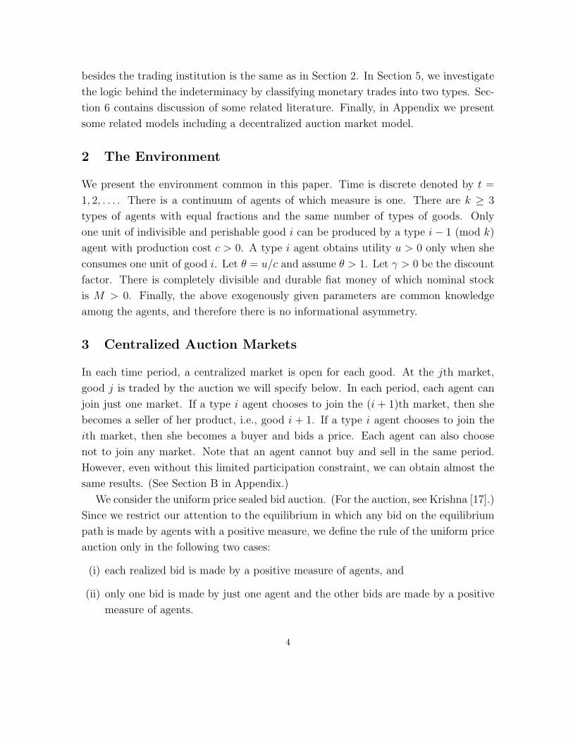
besides the trading institution is the same as in Section 2. In Section 5, we investigate

the logic behind the indeterminacy by classifying monetary trades into two types. Sec-

tion 6 contains discussion of some related literature. Finally, in Appendix we present

some related models including a decentralized auction market model.

2 The Environment

We present the environment common in this paper. Time is discrete denoted by t =

1, 2, . . . . There is a continuum of agents of which measure is one. There are k ≥ 3

types of agents with equal fractions and the same number of types of goods. Only

one unit of indivisible and perishable good i can be produced by a type i − 1 (mod k)

agent with production cost c > 0. A type i agent obtains utility u > 0 only when she

consumes one unit of good i. Let θ = u/c and assume θ > 1. Let γ > 0 be the discount

factor. There is completely divisible and durable fiat money of which nominal stock

is M > 0. Finally, the above exogenously given parameters are common knowledge

among the agents, and therefore there is no informational asymmetry.

3 Centralized Auction Markets

In each time period, a centralized market is open for each good. At the jth market,

good j is traded by the auction we will specify below. In each period, each agent can

join just one market. If a type i agent chooses to join the (i + 1)th market, then she

becomes a seller of her product, i.e., good i + 1. If a type i agent chooses to join the

ith market, then she becomes a buyer and bids a price. Each agent can also choose

not to join any market. Note that an agent cannot buy and sell in the same period.

However, even without this limited participation constraint, we can obtain almost the

same results. (See Section B in Appendix.)

We consider the uniform price sealed bid auction. (For the auction, see Krishna [17].)

Since we restrict our attention to the equilibrium in which any bid on the equilibrium

path is made by agents with a positive measure, we define the rule of the uniform price

auction only in the following two cases:

(i) each realized bid is made by a positive measure of agents, and

(ii) only one bid is made by just one agent and the other bids are made by a positive

measure of agents.

4

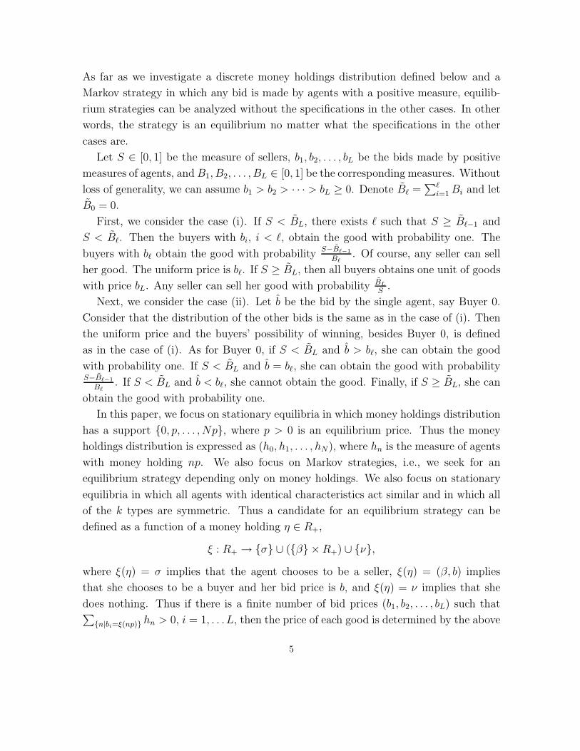
As far as we investigate a discrete money holdings distribution defined below and a

Markov strategy in which any bid is made by agents with a positive measure, equilib-

rium strategies can be analyzed without the specifications in the other cases. In other

words, the strategy is an equilibrium no matter what the specifications in the other

cases are.

Let S ∈ [0, 1] be the measure of sellers, b1, b2, . . . , bL be the bids made by positive

measures of agents, and B1, B2, . . . , BL ∈ [0, 1] be the corresponding measures. Without

loss of generality, we can assume b1 > b2 > · · · > bL ≥ 0. Denote B� =∑�

i=1 Bi and let

B0 = 0.

First, we consider the case (i). If S < BL, there exists � such that S ≥ B�−1 and

S < B�. Then the buyers with bi, i < �, obtain the good with probability one. The

buyers with b� obtain the good with probabilityS−B�−1

B�. Of course, any seller can sell

her good. The uniform price is b�. If S ≥ BL, then all buyers obtains one unit of goods

with price bL. Any seller can sell her good with probability BL

S.

Next, we consider the case (ii). Let b be the bid by the single agent, say Buyer 0.

Consider that the distribution of the other bids is the same as in the case of (i). Then

the uniform price and the buyers’ possibility of winning, besides Buyer 0, is defined

as in the case of (i). As for Buyer 0, if S < BL and b > b�, she can obtain the good

with probability one. If S < BL and b = b�, she can obtain the good with probabilityS−B�−1

B�. If S < BL and b < b�, she cannot obtain the good. Finally, if S ≥ BL, she can

obtain the good with probability one.

In this paper, we focus on stationary equilibria in which money holdings distribution

has a support {0, p, . . . , Np}, where p > 0 is an equilibrium price. Thus the money

holdings distribution is expressed as (h0, h1, . . . , hN), where hn is the measure of agents

with money holding np. We also focus on Markov strategies, i.e., we seek for an

equilibrium strategy depending only on money holdings. We also focus on stationary

equilibria in which all agents with identical characteristics act similar and in which all

of the k types are symmetric. Thus a candidate for an equilibrium strategy can be

defined as a function of a money holding η ∈ R+,

ξ : R+ → {σ} ∪ ({β} × R+) ∪ {ν},where ξ(η) = σ implies that the agent chooses to be a seller, ξ(η) = (β, b) implies

that she chooses to be a buyer and her bid price is b, and ξ(η) = ν implies that she

does nothing. Thus if there is a finite number of bid prices (b1, b2, . . . , bL) such that∑{n|bi=ξ(np)} hn > 0, i = 1, . . . L, then the price of each good is determined by the above

5

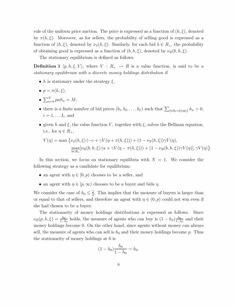
rule of the uniform price auction. The price is expressed as a function of (h, ξ), denoted

by π(h, ξ). Moreover, as for sellers, the probability of selling good is expressed as a

function of (h, ξ), denoted by νS(h, ξ). Similarly, for each bid b ∈ R+, the probability

of obtaining good is expressed as a function of (b, h, ξ), denoted by νB(b, h, ξ).

The stationary equilibrium is defined as follows.

Definition 1 〈p, h, ξ, V 〉, where V : R+ → R is a value function, is said to be a

stationary equilibrium with a discrete money holdings distribution if

• h is stationary under the strategy ξ,

• p = π(h, ξ),

• ∑Nn=0 pnhn = M ,

• there is a finite number of bid prices (b1, b2, . . . , bL) such that∑

{n|bi=ξ(np)} hn > 0,

i = 1, . . . L, and

• given h and ξ, the value function V , together with ξ, solves the Bellman equation,

i.e., for η ∈ R+,

V (η) = max{νS(h, ξ) (−c + γV (η + π(h, ξ))) + (1 − νS(h, ξ))γV (η),

maxb∈R+

[νB(b, h, ξ) (u + γV (η − π(h, ξ))) + (1 − νB(b, h, ξ))γV (η)], γV (η)}.

In this section, we focus on stationary equilibria with N = 1. We consider the

following strategy as a candidate for equilibrium:

• an agent with η ∈ [0, p) chooses to be a seller, and

• an agent with η ∈ [p,∞) chooses to be a buyer and bids η.

We consider the case of h0 ≤ 12. This implies that the measure of buyers is larger than

or equal to that of sellers, and therefore an agent with η ∈ (0, p) could not win even if

she had chosen to be a buyer.

The stationarity of money holdings distributions is expressed as follows. Since

νB(p, h, ξ) = h0

1−h0holds, the measure of agents who can buy is (1 − h0)

h0

1−h0and their

money holdings become 0. On the other hand, since agents without money can always

sell, the measure of agents who can sell is h0 and their money holdings become p. Thus

the stationarity of money holdings at 0 is

(1 − h0)h0

1 − h0= h0.

6

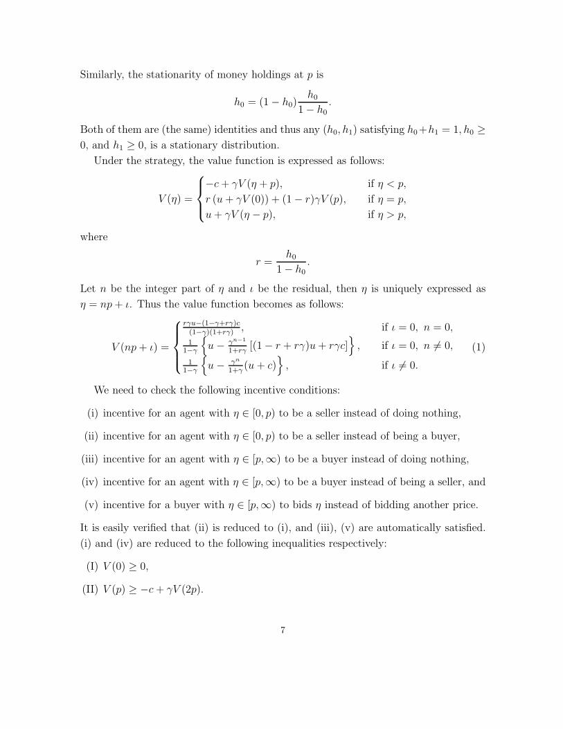
Similarly, the stationarity of money holdings at p is

h0 = (1 − h0)h0

1 − h0

.

Both of them are (the same) identities and thus any (h0, h1) satisfying h0+h1 = 1, h0 ≥0, and h1 ≥ 0, is a stationary distribution.

Under the strategy, the value function is expressed as follows:

V (η) =

⎧⎪⎨⎪⎩−c + γV (η + p), if η < p,

r (u + γV (0)) + (1 − r)γV (p), if η = p,

u + γV (η − p), if η > p,

where

r =h0

1 − h0.

Let n be the integer part of η and ι be the residual, then η is uniquely expressed as

η = np + ι. Thus the value function becomes as follows:

V (np + ι) =

⎧⎪⎪⎨⎪⎪⎩

rγu−(1−γ+rγ)c(1−γ)(1+rγ)

, if ι = 0, n = 0,

11−γ

{u − γn−1

1+rγ[(1 − r + rγ)u + rγc]

}, if ι = 0, n �= 0,

11−γ

{u − γn

1+γ(u + c)

}, if ι �= 0.

(1)

We need to check the following incentive conditions:

(i) incentive for an agent with η ∈ [0, p) to be a seller instead of doing nothing,

(ii) incentive for an agent with η ∈ [0, p) to be a seller instead of being a buyer,

(iii) incentive for an agent with η ∈ [p,∞) to be a buyer instead of doing nothing,

(iv) incentive for an agent with η ∈ [p,∞) to be a buyer instead of being a seller, and

(v) incentive for a buyer with η ∈ [p,∞) to bids η instead of bidding another price.

It is easily verified that (ii) is reduced to (i), and (iii), (v) are automatically satisfied.

(i) and (iv) are reduced to the following inequalities respectively:

(I) V (0) ≥ 0,

(II) V (p) ≥ −c + γV (2p).

7

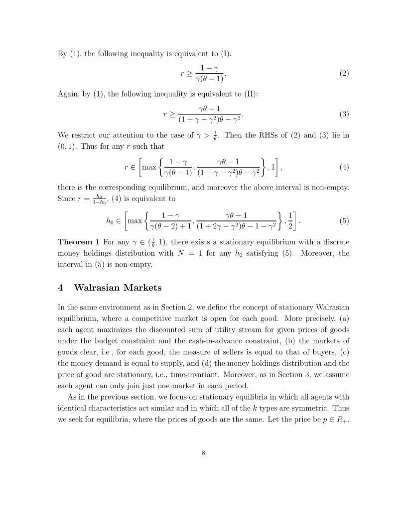
By (1), the following inequality is equivalent to (I):

r ≥ 1 − γ

γ(θ − 1). (2)

Again, by (1), the following inequality is equivalent to (II):

r ≥ γθ − 1

(1 + γ − γ2)θ − γ2. (3)

We restrict our attention to the case of γ > 1θ. Then the RHSs of (2) and (3) lie in

(0, 1). Thus for any r such that

r ∈[max

{1 − γ

γ(θ − 1),

γθ − 1

(1 + γ − γ2)θ − γ2

}, 1

], (4)

there is the corresponding equilibrium, and moreover the above interval is non-empty.

Since r = h0

1−h0, (4) is equivalent to

h0 ∈[max

{1 − γ

γ(θ − 2) + 1,

γθ − 1

(1 + 2γ − γ2)θ − 1 − γ2

},1

2

]. (5)

Theorem 1 For any γ ∈ (1θ, 1), there exists a stationary equilibrium with a discrete

money holdings distribution with N = 1 for any h0 satisfying (5). Moreover, the

interval in (5) is non-empty.

4 Walrasian Markets

In the same environment as in Section 2, we define the concept of stationary Walrasian

equilibrium, where a competitive market is open for each good. More precisely, (a)

each agent maximizes the discounted sum of utility stream for given prices of goods

under the budget constraint and the cash-in-advance constraint, (b) the markets of

goods clear, i.e., for each good, the measure of sellers is equal to that of buyers, (c)

the money demand is equal to supply, and (d) the money holdings distribution and the

price of good are stationary, i.e., time-invariant. Moreover, as in Section 3, we assume

each agent can only join just one market in each period.

As in the previous section, we focus on stationary equilibria in which all agents with

identical characteristics act similar and in which all of the k types are symmetric. Thus

we seek for equilibria, where the prices of goods are the same. Let the price be p ∈ R+.

8

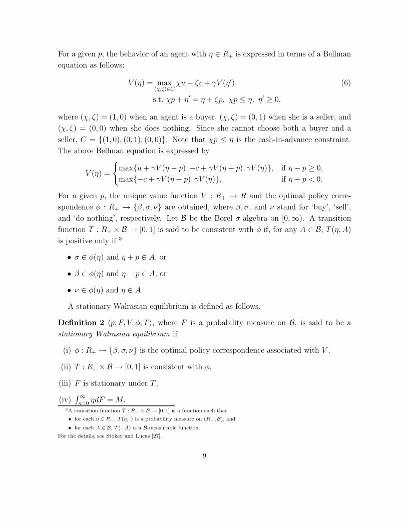
For a given p, the behavior of an agent with η ∈ R+ is expressed in terms of a Bellman

equation as follows:

V (η) = max(χ,ζ)∈C

χu − ζc + γV (η′), (6)

s.t. χp + η′ = η + ζp, χp ≤ η, η′ ≥ 0,

where (χ, ζ) = (1, 0) when an agent is a buyer, (χ, ζ) = (0, 1) when she is a seller, and

(χ, ζ) = (0, 0) when she does nothing. Since she cannot choose both a buyer and a

seller, C = {(1, 0), (0, 1), (0, 0)}. Note that χp ≤ η is the cash-in-advance constraint.

The above Bellman equation is expressed by

V (η) =

{max{u + γV (η − p),−c + γV (η + p), γV (η)}, if η − p ≥ 0,

max{−c + γV (η + p), γV (η)}, if η − p < 0.

For a given p, the unique value function V : R+ → R and the optimal policy corre-

spondence φ : R+ → {β, σ, ν} are obtained, where β, σ, and ν stand for ‘buy’, ‘sell’,

and ‘do nothing’, respectively. Let B be the Borel σ-algebra on [0,∞). A transition

function T : R+ × B → [0, 1] is said to be consistent with φ if, for any A ∈ B, T (η, A)

is positive only if 3

• σ ∈ φ(η) and η + p ∈ A, or

• β ∈ φ(η) and η − p ∈ A, or

• ν ∈ φ(η) and η ∈ A.

A stationary Walrasian equilibrium is defined as follows.

Definition 2 〈p, F, V, φ, T 〉, where F is a probability measure on B, is said to be a

stationary Walrasian equilibrium if

(i) φ : R+ → {β, σ, ν} is the optimal policy correspondence associated with V ,

(ii) T : R+ × B → [0, 1] is consistent with φ,

(iii) F is stationary under T ,

(iv)∫ ∞

n=0ηdF = M ,

3A transition function T : R+ ×B → [0, 1] is a function such that

• for each η ∈ R+, T (η, ·) is a probability measure on (R+,B), and

• for each A ∈ B, T (·, A) is a B-measurable function.

For the details, see Stokey and Lucas [27].

9

(v) given p, V satisfies (6),

(vi) T (η, {η − p}) and T (η, {η + p}) are measurable functions of η, and∫T (η, {η − p})dF =

∫T (η, {η + p})dF

holds.

As for (i)-(v), no explanation is needed. (vi) is the market clearing condition for goods;

namely, the measure of buyers is equal to that of sellers. Note that, by Walras’ law,

money demand is equal to money supply if (vi) is satisfied.

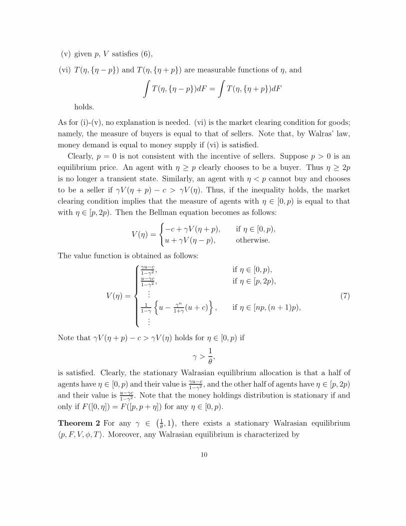
Clearly, p = 0 is not consistent with the incentive of sellers. Suppose p > 0 is an

equilibrium price. An agent with η ≥ p clearly chooses to be a buyer. Thus η ≥ 2p

is no longer a transient state. Similarly, an agent with η < p cannot buy and chooses

to be a seller if γV (η + p) − c > γV (η). Thus, if the inequality holds, the market

clearing condition implies that the measure of agents with η ∈ [0, p) is equal to that

with η ∈ [p, 2p). Then the Bellman equation becomes as follows:

V (η) =

{−c + γV (η + p), if η ∈ [0, p),

u + γV (η − p), otherwise.

The value function is obtained as follows:

V (η) =

⎧⎪⎪⎪⎪⎪⎪⎪⎨⎪⎪⎪⎪⎪⎪⎪⎩

γu−c1−γ2 , if η ∈ [0, p),u−γc1−γ2 , if η ∈ [p, 2p),

...1

1−γ

{u − γn

1+γ(u + c)

}, if η ∈ [np, (n + 1)p),

...

(7)

Note that γV (η + p) − c > γV (η) holds for η ∈ [0, p) if

γ >1

θ,

is satisfied. Clearly, the stationary Walrasian equilibrium allocation is that a half of

agents have η ∈ [0, p) and their value is γu−c1−γ2 , and the other half of agents have η ∈ [p, 2p)

and their value is u−γc1−γ2 . Note that the money holdings distribution is stationary if and

only if F ([0, η]) = F ([p, p + η]) for any η ∈ [0, p).

Theorem 2 For any γ ∈ (1θ, 1

), there exists a stationary Walrasian equilibrium

〈p, F, V, φ, T 〉. Moreover, any Walrasian equilibrium is characterized by

10

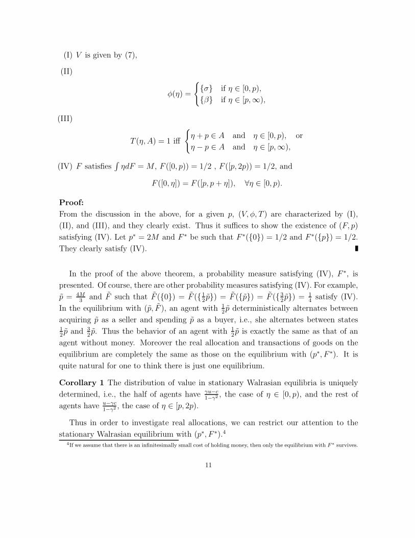
(I) V is given by (7),

(II)

φ(η) =

{{σ} if η ∈ [0, p),

{β} if η ∈ [p,∞),

(III)

T (η, A) = 1 iff

{η + p ∈ A and η ∈ [0, p), or

η − p ∈ A and η ∈ [p,∞),

(IV) F satisfies∫

ηdF = M , F ([0, p)) = 1/2 , F ([p, 2p)) = 1/2, and

F ([0, η]) = F ([p, p + η]), ∀η ∈ [0, p).

Proof:

From the discussion in the above, for a given p, (V, φ, T ) are characterized by (I),

(II), and (III), and they clearly exist. Thus it suffices to show the existence of (F, p)

satisfying (IV). Let p∗ = 2M and F ∗ be such that F ∗({0}) = 1/2 and F ∗({p}) = 1/2.

They clearly satisfy (IV).

In the proof of the above theorem, a probability measure satisfying (IV), F ∗, is

presented. Of course, there are other probability measures satisfying (IV). For example,

p = 4M3

and F such that F ({0}) = F ({12p}) = F ({p}) = F ({3

2p}) = 1

4satisfy (IV).

In the equilibrium with (p, F ), an agent with 12p deterministically alternates between

acquiring p as a seller and spending p as a buyer, i.e., she alternates between states12p and 3

2p. Thus the behavior of an agent with 1

2p is exactly the same as that of an

agent without money. Moreover the real allocation and transactions of goods on the

equilibrium are completely the same as those on the equilibrium with (p∗, F ∗). It is

quite natural for one to think there is just one equilibrium.

Corollary 1 The distribution of value in stationary Walrasian equilibria is uniquely

determined, i.e., the half of agents have γu−c1−γ2 , the case of η ∈ [0, p), and the rest of

agents have u−γc1−γ2 , the case of η ∈ [p, 2p).

Thus in order to investigate real allocations, we can restrict our attention to the

stationary Walrasian equilibrium with (p∗, F ∗).44If we assume that there is an infinitesimally small cost of holding money, then only the equilibrium with F ∗ survives.

11

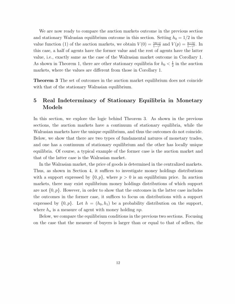
We are now ready to compare the auction markets outcome in the previous section

and stationary Walrasian equilibrium outcome in this section. Setting h0 = 1/2 in the

value function (1) of the auction markets, we obtain V (0) = γu−c1−γ2 and V (p) = u−γc

1−γ2 . In

this case, a half of agents have the former value and the rest of agents have the latter

value, i.e., exactly same as the case of the Walrasian market outcome in Corollary 1.

As shown in Theorem 1, there are other stationary equilibria for h0 < 12

in the auction

markets, where the values are different from those in Corollary 1.

Theorem 3 The set of outcomes in the auction market equilibrium does not coincide

with that of the stationary Walrasian equilibrium.

5 Real Indeterminacy of Stationary Equilibria in MonetaryModels

In this section, we explore the logic behind Theorem 3. As shown in the previous

sections, the auction markets have a continuum of stationary equilibria, while the

Walrasian markets have the unique equilibrium, and thus the outcomes do not coincide.

Below, we show that there are two types of fundamental natures of monetary trades,

and one has a continuum of stationary equilibrium and the other has locally unique

equilibria. Of course, a typical example of the former case is the auction market and

that of the latter case is the Walrasian market.

In the Walrasian market, the price of goods is determined in the centralized markets.

Thus, as shown in Section 4, it suffices to investigate money holdings distributions

with a support expressed by {0, p}, where p > 0 is an equilibrium price. In auction

markets, there may exist equilibrium money holdings distributions of which support

are not {0, p}. However, in order to show that the outcomes in the latter case includes

the outcomes in the former case, it suffices to focus on distributions with a support

expressed by {0, p}. Let h = (h0, h1) be a probability distribution on the support,

where hn is a measure of agent with money holding np.

Below, we compare the equilibrium conditions in the previous two sections. Focusing

on the case that the measure of buyers is larger than or equal to that of sellers, the

12

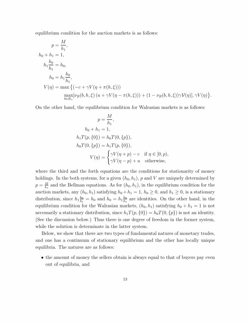
equilibrium condition for the auction markets is as follows:

p =M

h1

,

h0 + h1 = 1,

h1h0

h1= h0,

h0 = h1h0

h1,

V (η) = max{(−c + γV (η + π(h, ξ)))

maxb∈R+

[νB(b, h, ξ) (u + γV (η − π(h, ξ))) + (1 − νB(b, h, ξ))γV(η)], γV (η)}.

On the other hand, the equilibrium condition for Walrasian markets is as follows:

p =M

h1

,

h0 + h1 = 1,

h1T (p, {0}) = h0T (0, {p}),h0T (0, {p}) = h1T (p, {0}),

V (η) =

{γV (η + p) − c if η ∈ [0, p),

γV (η − p) + u otherwise,

where the third and the forth equations are the conditions for stationarity of money

holdings. In the both systems, for a given (h0, h1), p and V are uniquely determined by

p = Mh1

and the Bellman equations. As for (h0, h1), in the equilibrium condition for the

auction markets, any (h0, h1) satisfying h0 +h1 = 1, h0 ≥ 0, and h1 ≥ 0, is a stationary

distribution, since h1h0

h1= h0 and h0 = h1

h0

h1are identities. On the other hand, in the

equilibrium condition for the Walrasian markets, (h0, h1) satisfying h0 + h1 = 1 is not

necessarily a stationary distribution, since h1T (p, {0}) = h0T (0, {p}) is not an identity.

(See the discussion below.) Thus there is one degree of freedom in the former system,

while the solution is determinate in the latter system.

Below, we show that there are two types of fundamental natures of monetary trades,

and one has a continuum of stationary equilibrium and the other has locally unique

equilibria. The natures are as follows:

• the amount of money the sellers obtain is always equal to that of buyers pay even

out of equilibria, and

13

• the amount of money the sellers obtain is not necessarily equal to that of buyers

pay.

The auction market is clearly classified as the first type and the Walrasian market is

classified as the second type. Indeed, in the auction markets, the amount of money the

sellers obtain is ph0 and that of buyers pay is ph1h0

h1= ph0. By this identity, any money

holdings distribution is stationary, i.e., all (h0, h1) satisfying h0 + h1 = 1, h0 ≥ 0, and

h1 ≥ 0 is stationarity, and the set of equilibria is a continuum. On the other hand, in

the Walrasian markets, if p is large enough, then all agents without money choose to

be sellers, i.e., T (0, {p}) = 1, and the amount of money the sellers obtain is ph0 and

the amount of money the buyers pay is at most p(1 − h0). Of course, they are not

necessarily the same.

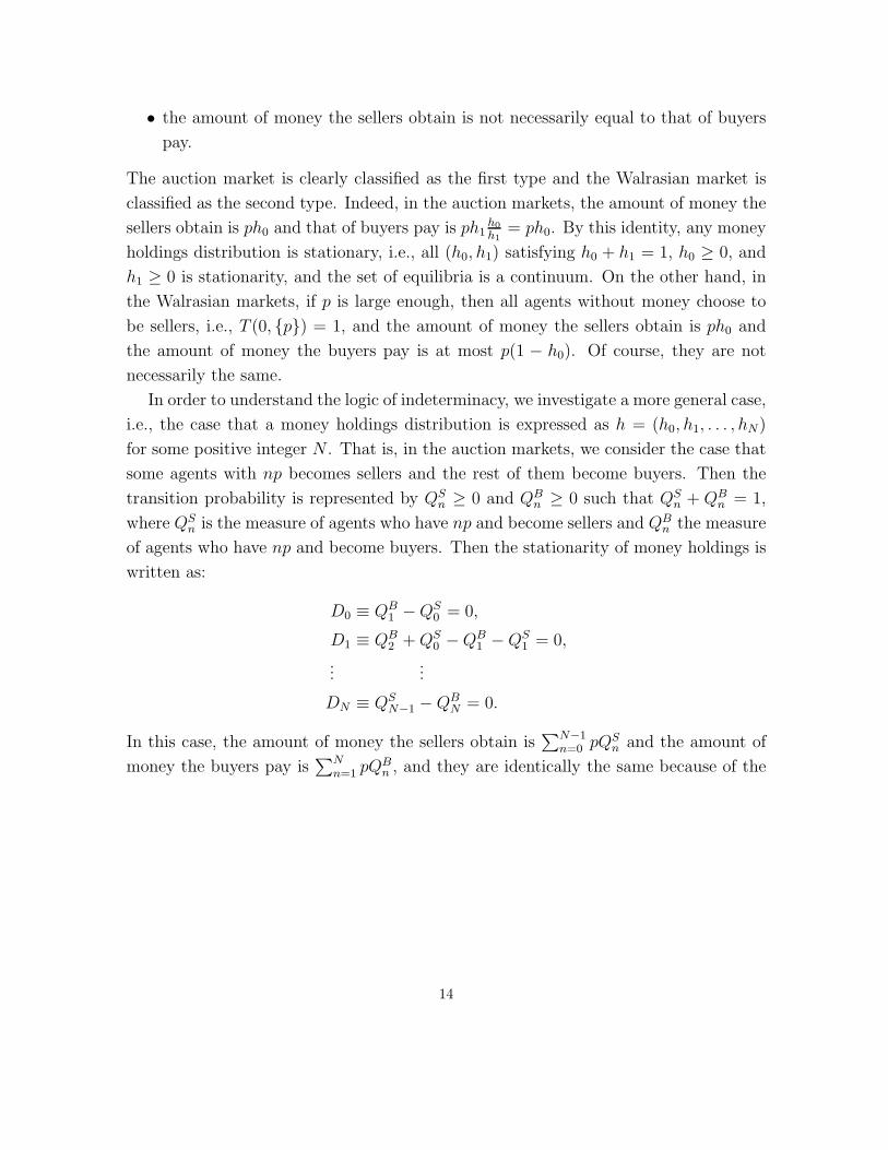
In order to understand the logic of indeterminacy, we investigate a more general case,

i.e., the case that a money holdings distribution is expressed as h = (h0, h1, . . . , hN)

for some positive integer N . That is, in the auction markets, we consider the case that

some agents with np becomes sellers and the rest of them become buyers. Then the

transition probability is represented by QSn ≥ 0 and QB

n ≥ 0 such that QSn + QB

n = 1,

where QSn is the measure of agents who have np and become sellers and QB

n the measure

of agents who have np and become buyers. Then the stationarity of money holdings is

written as:

D0 ≡ QB1 − QS

0 = 0,

D1 ≡ QB2 + QS

0 − QB1 − QS

1 = 0,

......

DN ≡ QSN−1 − QB

N = 0.

In this case, the amount of money the sellers obtain is∑N−1

n=0 pQSn and the amount of

money the buyers pay is∑N

n=1 pQBn , and they are identically the same because of the

14

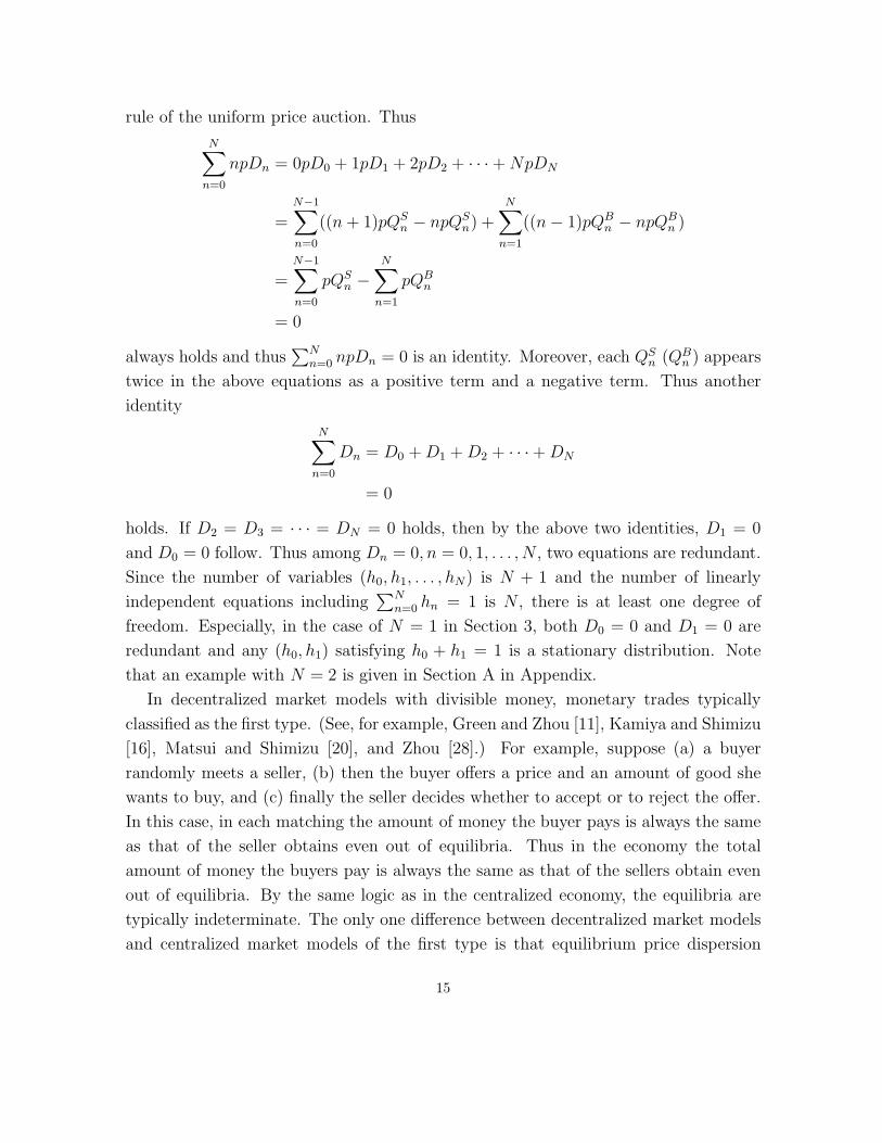
rule of the uniform price auction. Thus

N∑n=0

npDn = 0pD0 + 1pD1 + 2pD2 + · · · + NpDN

=

N−1∑n=0

((n + 1)pQSn − npQS

n) +

N∑n=1

((n − 1)pQBn − npQB

n )

=N−1∑n=0

pQSn −

N∑n=1

pQBn

= 0

always holds and thus∑N

n=0 npDn = 0 is an identity. Moreover, each QSn (QB

n ) appears

twice in the above equations as a positive term and a negative term. Thus another

identity

N∑n=0

Dn = D0 + D1 + D2 + · · ·+ DN

= 0

holds. If D2 = D3 = · · · = DN = 0 holds, then by the above two identities, D1 = 0

and D0 = 0 follow. Thus among Dn = 0, n = 0, 1, . . . , N , two equations are redundant.

Since the number of variables (h0, h1, . . . , hN) is N + 1 and the number of linearly

independent equations including∑N

n=0 hn = 1 is N , there is at least one degree of

freedom. Especially, in the case of N = 1 in Section 3, both D0 = 0 and D1 = 0 are

redundant and any (h0, h1) satisfying h0 + h1 = 1 is a stationary distribution. Note

that an example with N = 2 is given in Section A in Appendix.

In decentralized market models with divisible money, monetary trades typically

classified as the first type. (See, for example, Green and Zhou [11], Kamiya and Shimizu

[16], Matsui and Shimizu [20], and Zhou [28].) For example, suppose (a) a buyer

randomly meets a seller, (b) then the buyer offers a price and an amount of good she

wants to buy, and (c) finally the seller decides whether to accept or to reject the offer.

In this case, in each matching the amount of money the buyer pays is always the same

as that of the seller obtains even out of equilibria. Thus in the economy the total

amount of money the buyers pay is always the same as that of the sellers obtain even

out of equilibria. By the same logic as in the centralized economy, the equilibria are

typically indeterminate. The only one difference between decentralized market models

and centralized market models of the first type is that equilibrium price dispersion

15

might occur in decentralized market models. (See Kamiya and Sato [15] and Matsui

and Shimizu [20].)

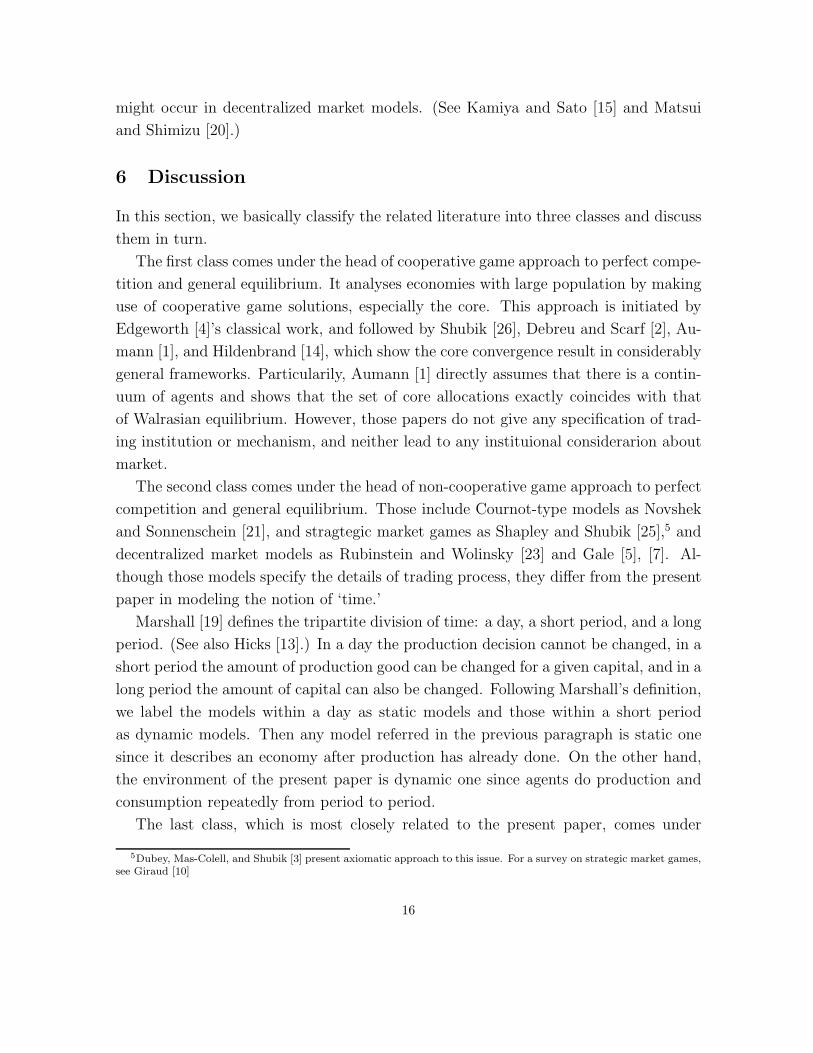
6 Discussion

In this section, we basically classify the related literature into three classes and discuss

them in turn.

The first class comes under the head of cooperative game approach to perfect compe-

tition and general equilibrium. It analyses economies with large population by making

use of cooperative game solutions, especially the core. This approach is initiated by

Edgeworth [4]’s classical work, and followed by Shubik [26], Debreu and Scarf [2], Au-

mann [1], and Hildenbrand [14], which show the core convergence result in considerably

general frameworks. Particularily, Aumann [1] directly assumes that there is a contin-

uum of agents and shows that the set of core allocations exactly coincides with that

of Walrasian equilibrium. However, those papers do not give any specification of trad-

ing institution or mechanism, and neither lead to any instituional considerarion about

market.

The second class comes under the head of non-cooperative game approach to perfect

competition and general equilibrium. Those include Cournot-type models as Novshek

and Sonnenschein [21], and stragtegic market games as Shapley and Shubik [25],5 and

decentralized market models as Rubinstein and Wolinsky [23] and Gale [5], [7]. Al-

though those models specify the details of trading process, they differ from the present

paper in modeling the notion of ‘time.’

Marshall [19] defines the tripartite division of time: a day, a short period, and a long

period. (See also Hicks [13].) In a day the production decision cannot be changed, in a

short period the amount of production good can be changed for a given capital, and in a

long period the amount of capital can also be changed. Following Marshall’s definition,

we label the models within a day as static models and those within a short period

as dynamic models. Then any model referred in the previous paragraph is static one

since it describes an economy after production has already done. On the other hand,

the environment of the present paper is dynamic one since agents do production and

consumption repeatedly from period to period.

The last class, which is most closely related to the present paper, comes under

5Dubey, Mas-Colell, and Shubik [3] present axiomatic approach to this issue. For a survey on strategic market games,see Giraud [10]

16

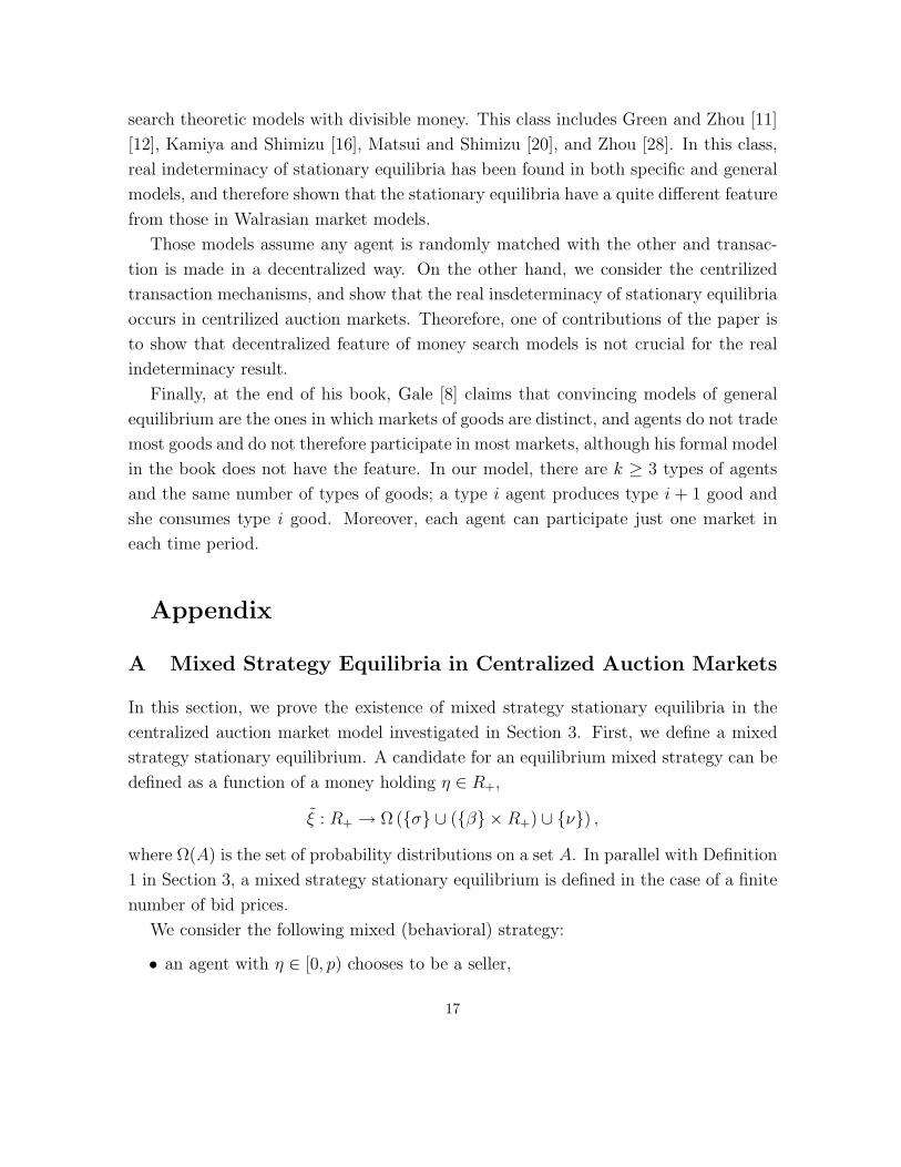
search theoretic models with divisible money. This class includes Green and Zhou [11]

[12], Kamiya and Shimizu [16], Matsui and Shimizu [20], and Zhou [28]. In this class,

real indeterminacy of stationary equilibria has been found in both specific and general

models, and therefore shown that the stationary equilibria have a quite different feature

from those in Walrasian market models.

Those models assume any agent is randomly matched with the other and transac-

tion is made in a decentralized way. On the other hand, we consider the centrilized

transaction mechanisms, and show that the real insdeterminacy of stationary equilibria

occurs in centrilized auction markets. Theorefore, one of contributions of the paper is

to show that decentralized feature of money search models is not crucial for the real

indeterminacy result.

Finally, at the end of his book, Gale [8] claims that convincing models of general

equilibrium are the ones in which markets of goods are distinct, and agents do not trade

most goods and do not therefore participate in most markets, although his formal model

in the book does not have the feature. In our model, there are k ≥ 3 types of agents

and the same number of types of goods; a type i agent produces type i + 1 good and

she consumes type i good. Moreover, each agent can participate just one market in

each time period.

Appendix

A Mixed Strategy Equilibria in Centralized Auction Markets

In this section, we prove the existence of mixed strategy stationary equilibria in the

centralized auction market model investigated in Section 3. First, we define a mixed

strategy stationary equilibrium. A candidate for an equilibrium mixed strategy can be

defined as a function of a money holding η ∈ R+,

ξ : R+ → Ω ({σ} ∪ ({β} × R+) ∪ {ν}) ,

where Ω(A) is the set of probability distributions on a set A. In parallel with Definition

1 in Section 3, a mixed strategy stationary equilibrium is defined in the case of a finite

number of bid prices.

We consider the following mixed (behavioral) strategy:

• an agent with η ∈ [0, p) chooses to be a seller,

17

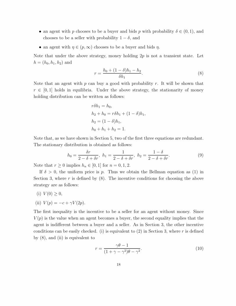
• an agent with p chooses to be a buyer and bids p with probability δ ∈ (0, 1), and

chooses to be a seller with probability 1 − δ, and

• an agent with η ∈ (p,∞) chooses to be a buyer and bids η.

Note that under the above strategy, money holding 2p is not a transient state. Let

h = (h0, h1, h2) and

r =h0 + (1 − δ)h1 − h2

δh1. (8)

Note that an agent with p can buy a good with probability r. It will be shown that

r ∈ [0, 1] holds in equilibria. Under the above strategy, the stationarity of money

holding distribution can be written as follows:

rδh1 = h0,

h2 + h0 = rδh1 + (1 − δ)h1,

h2 = (1 − δ)h1,

h0 + h1 + h2 = 1.

Note that, as we have shown in Section 5, two of the first three equations are redundant.

The stationary distribution is obtained as follows:

h0 =δr

2 − δ + δr, h1 =

1

2 − δ + δr, h2 =

1 − δ

2 − δ + δr. (9)

Note that r ≥ 0 implies hn ∈ [0, 1] for n = 0, 1, 2.

If δ > 0, the uniform price is p. Thus we obtain the Bellman equation as (1) in

Section 3, where r is defined by (8). The incentive conditions for choosing the above

strategy are as follows:

(i) V (0) ≥ 0,

(ii) V (p) = −c + γV (2p).

The first inequality is the incentive to be a seller for an agent without money. Since

V (p) is the value when an agent becomes a buyer, the second equality implies that the

agent is indifferent between a buyer and a seller. As in Section 3, the other incentive

conditions can be easily checked. (i) is equivalent to (2) in Section 3, where r is defined

by (8), and (ii) is equivalent to

r =γθ − 1

(1 + γ − γ2)θ − γ2. (10)

18

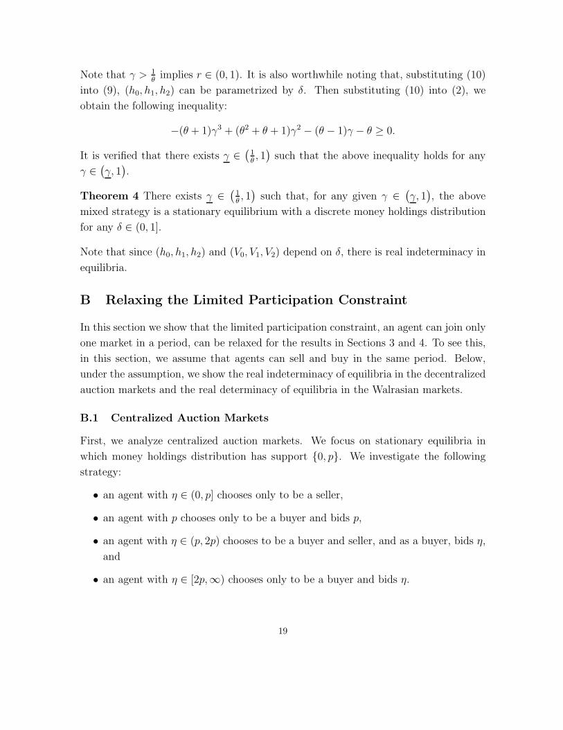
Note that γ > 1θ

implies r ∈ (0, 1). It is also worthwhile noting that, substituting (10)

into (9), (h0, h1, h2) can be parametrized by δ. Then substituting (10) into (2), we

obtain the following inequality:

−(θ + 1)γ3 + (θ2 + θ + 1)γ2 − (θ − 1)γ − θ ≥ 0.

It is verified that there exists γ ∈ (1θ, 1

)such that the above inequality holds for any

γ ∈ (γ, 1

).

Theorem 4 There exists γ ∈ (1θ, 1

)such that, for any given γ ∈ (

γ, 1), the above

mixed strategy is a stationary equilibrium with a discrete money holdings distribution

for any δ ∈ (0, 1].

Note that since (h0, h1, h2) and (V0, V1, V2) depend on δ, there is real indeterminacy in

equilibria.

B Relaxing the Limited Participation Constraint

In this section we show that the limited participation constraint, an agent can join only

one market in a period, can be relaxed for the results in Sections 3 and 4. To see this,

in this section, we assume that agents can sell and buy in the same period. Below,

under the assumption, we show the real indeterminacy of equilibria in the decentralized

auction markets and the real determinacy of equilibria in the Walrasian markets.

B.1 Centralized Auction Markets

First, we analyze centralized auction markets. We focus on stationary equilibria in

which money holdings distribution has support {0, p}. We investigate the following

strategy:

• an agent with η ∈ (0, p] chooses only to be a seller,

• an agent with p chooses only to be a buyer and bids p,

• an agent with η ∈ (p, 2p) chooses to be a buyer and seller, and as a buyer, bids η,

and

• an agent with η ∈ [2p,∞) chooses only to be a buyer and bids η.

19

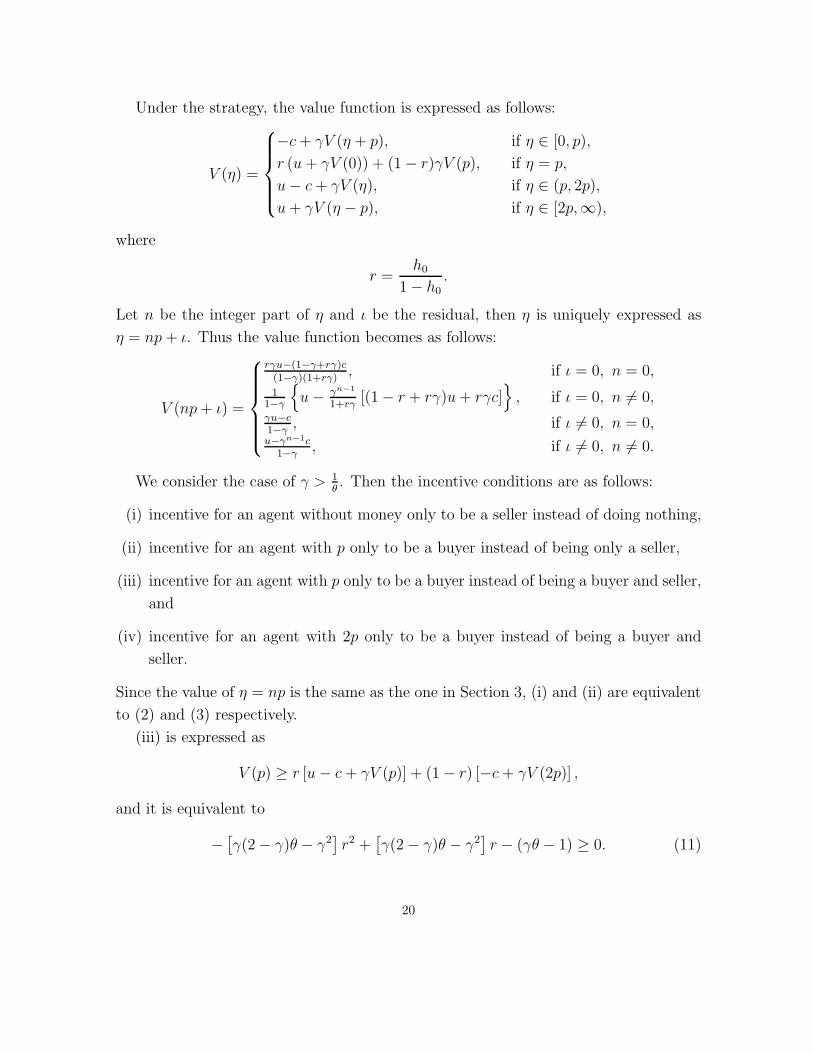
Under the strategy, the value function is expressed as follows:

V (η) =

⎧⎪⎪⎪⎨⎪⎪⎪⎩−c + γV (η + p), if η ∈ [0, p),

r (u + γV (0)) + (1 − r)γV (p), if η = p,

u − c + γV (η), if η ∈ (p, 2p),

u + γV (η − p), if η ∈ [2p,∞),

where

r =h0

1 − h0

.

Let n be the integer part of η and ι be the residual, then η is uniquely expressed as

η = np + ι. Thus the value function becomes as follows:

V (np + ι) =

⎧⎪⎪⎪⎪⎨⎪⎪⎪⎪⎩

rγu−(1−γ+rγ)c(1−γ)(1+rγ)

, if ι = 0, n = 0,

11−γ

{u − γn−1

1+rγ[(1 − r + rγ)u + rγc]

}, if ι = 0, n �= 0,

γu−c1−γ

, if ι �= 0, n = 0,u−γn−1c

1−γ, if ι �= 0, n �= 0.

We consider the case of γ > 1θ. Then the incentive conditions are as follows:

(i) incentive for an agent without money only to be a seller instead of doing nothing,

(ii) incentive for an agent with p only to be a buyer instead of being only a seller,

(iii) incentive for an agent with p only to be a buyer instead of being a buyer and seller,

and

(iv) incentive for an agent with 2p only to be a buyer instead of being a buyer and

seller.

Since the value of η = np is the same as the one in Section 3, (i) and (ii) are equivalent

to (2) and (3) respectively.

(iii) is expressed as

V (p) ≥ r [u − c + γV (p)] + (1 − r) [−c + γV (2p)] ,

and it is equivalent to

− [γ(2 − γ)θ − γ2

]r2 +

[γ(2 − γ)θ − γ2

]r − (γθ − 1) ≥ 0. (11)

20

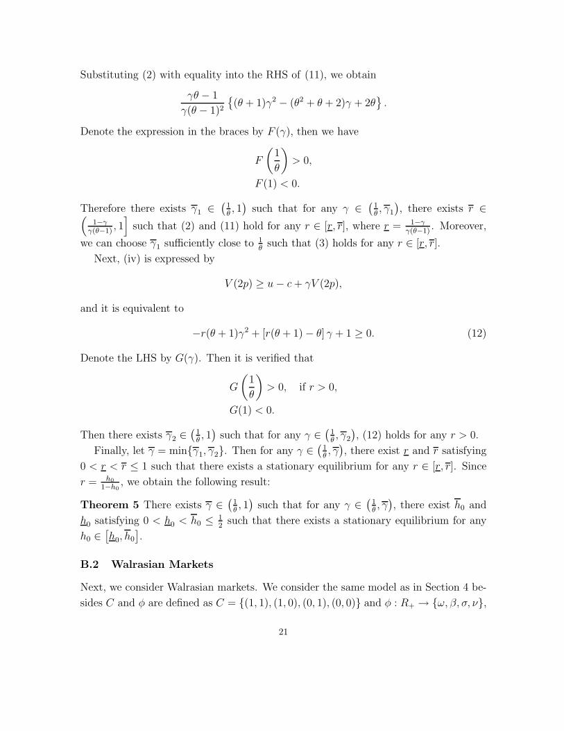
Substituting (2) with equality into the RHS of (11), we obtain

γθ − 1

γ(θ − 1)2

{(θ + 1)γ2 − (θ2 + θ + 2)γ + 2θ

}.

Denote the expression in the braces by F (γ), then we have

F

(1

θ

)> 0,

F (1) < 0.

Therefore there exists γ1 ∈ (1θ, 1

)such that for any γ ∈ (

1θ, γ1

), there exists r ∈(

1−γγ(θ−1)

, 1]

such that (2) and (11) hold for any r ∈ [r, r], where r = 1−γγ(θ−1)

. Moreover,

we can choose γ1 sufficiently close to 1θ

such that (3) holds for any r ∈ [r, r].

Next, (iv) is expressed by

V (2p) ≥ u − c + γV (2p),

and it is equivalent to

−r(θ + 1)γ2 + [r(θ + 1) − θ] γ + 1 ≥ 0. (12)

Denote the LHS by G(γ). Then it is verified that

G

(1

θ

)> 0, if r > 0,

G(1) < 0.

Then there exists γ2 ∈(

1θ, 1

)such that for any γ ∈ (

1θ, γ2

), (12) holds for any r > 0.

Finally, let γ = min{γ1, γ2}. Then for any γ ∈ (1θ, γ

), there exist r and r satisfying

0 < r < r ≤ 1 such that there exists a stationary equilibrium for any r ∈ [r, r]. Since

r = h0

1−h0, we obtain the following result:

Theorem 5 There exists γ ∈ (1θ, 1

)such that for any γ ∈ (

1θ, γ

), there exist h0 and

h0 satisfying 0 < h0 < h0 ≤ 12

such that there exists a stationary equilibrium for any

h0 ∈[h0, h0

].

B.2 Walrasian Markets

Next, we consider Walrasian markets. We consider the same model as in Section 4 be-

sides C and φ are defined as C = {(1, 1), (1, 0), (0, 1), (0, 0)} and φ : R+ → {ω, β, σ, ν},

21

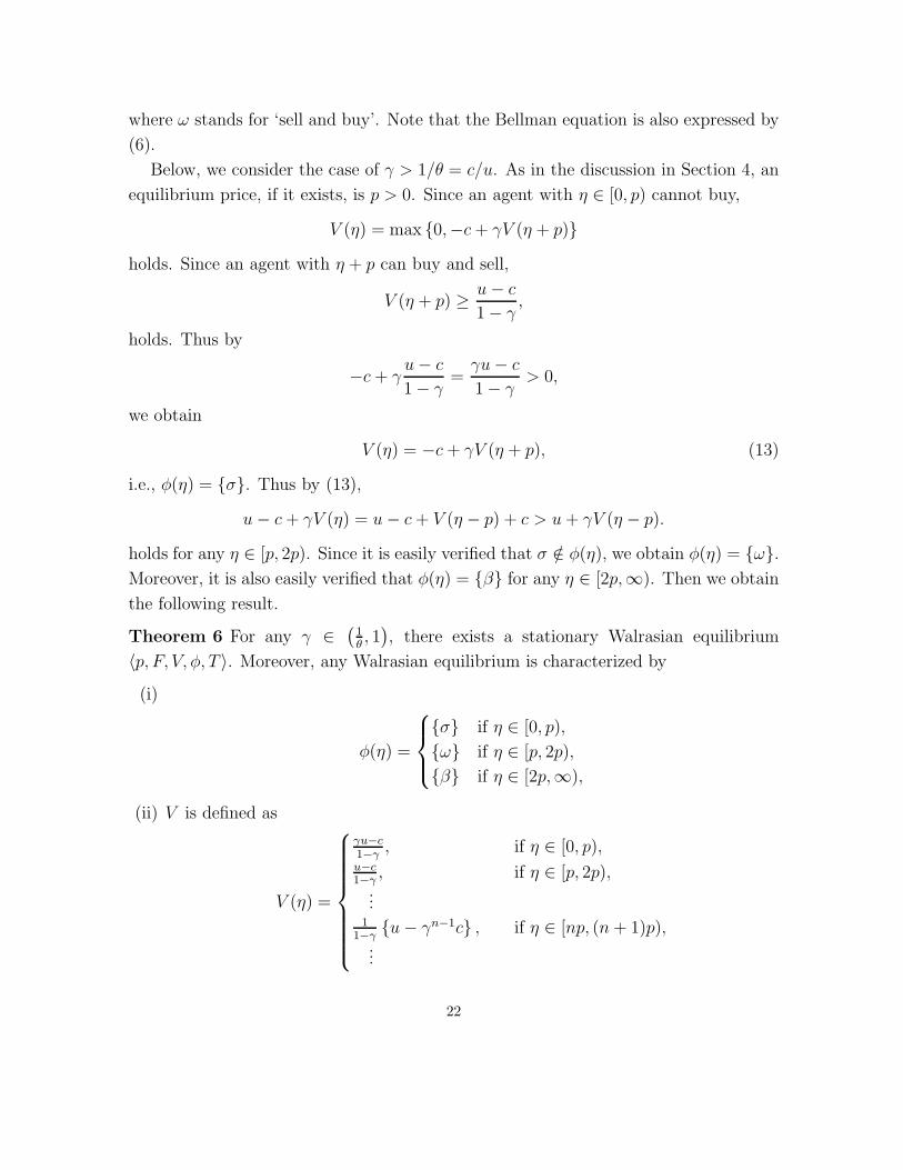
where ω stands for ‘sell and buy’. Note that the Bellman equation is also expressed by

(6).

Below, we consider the case of γ > 1/θ = c/u. As in the discussion in Section 4, an

equilibrium price, if it exists, is p > 0. Since an agent with η ∈ [0, p) cannot buy,

V (η) = max {0,−c + γV (η + p)}holds. Since an agent with η + p can buy and sell,

V (η + p) ≥ u − c

1 − γ,

holds. Thus by

−c + γu − c

1 − γ=

γu − c

1 − γ> 0,

we obtain

V (η) = −c + γV (η + p), (13)

i.e., φ(η) = {σ}. Thus by (13),

u − c + γV (η) = u − c + V (η − p) + c > u + γV (η − p).

holds for any η ∈ [p, 2p). Since it is easily verified that σ /∈ φ(η), we obtain φ(η) = {ω}.Moreover, it is also easily verified that φ(η) = {β} for any η ∈ [2p,∞). Then we obtain

the following result.

Theorem 6 For any γ ∈ (1θ, 1

), there exists a stationary Walrasian equilibrium

〈p, F, V, φ, T 〉. Moreover, any Walrasian equilibrium is characterized by

(i)

φ(η) =

⎧⎪⎨⎪⎩{σ} if η ∈ [0, p),

{ω} if η ∈ [p, 2p),

{β} if η ∈ [2p,∞),

(ii) V is defined as

V (η) =

⎧⎪⎪⎪⎪⎪⎪⎪⎨⎪⎪⎪⎪⎪⎪⎪⎩

γu−c1−γ

, if η ∈ [0, p),u−c1−γ

, if η ∈ [p, 2p),...

11−γ

{u − γn−1c} , if η ∈ [np, (n + 1)p),...

22

(iii)

T (η, A) = 1, iff

⎧⎪⎨⎪⎩

η + p ∈ A and η ∈ [0, p), or

η ∈ A and η ∈ [p, 2p), or

η − p ∈ A and η ∈ [2p,∞),

(iv) F satisfies

F ([p, 2p)) = 1,∫ 2p

p

ηdF = M.

Corollary 2 The distribution of value in stationary Walrasian equilibria is uniquely

determined, i.e., the value of any agent is u−c1−γ

.

The above corollary implies that the indeterminacy is not a real one but a nominal

one as in Section 4.

C Decentralized Auctions

In the same environment as in Section 2, we consider an economy, where trades take

place in decentralized second price auction markets, and show that there is also a

continuum of stationary equilibria.

In each period, each agent first chooses whether to be a seller or a buyer (or doing

nothing). Each seller posts a minimum bid of her second-price auction.6 After observing

the distribution of posted minimum bids, each buyer simultaneously chooses which

auction he participates in. After observing the number of the other participants in the

auction he participates in and bids a price.

In the environment, we consider the following strategy:

• an agent with η ∈ [0, p) chooses to be a seller and post a minimum bid p,

• an agent with p chooses to be a buyer and always bids p,

• an agent with η ∈ [p,∞) chooses to be a buyer, and

– bids p if there is no participant in the auction,

– bids η if there are other participants in the auction.6Nothing would change if we assume the sellers also choose her auction format.

23

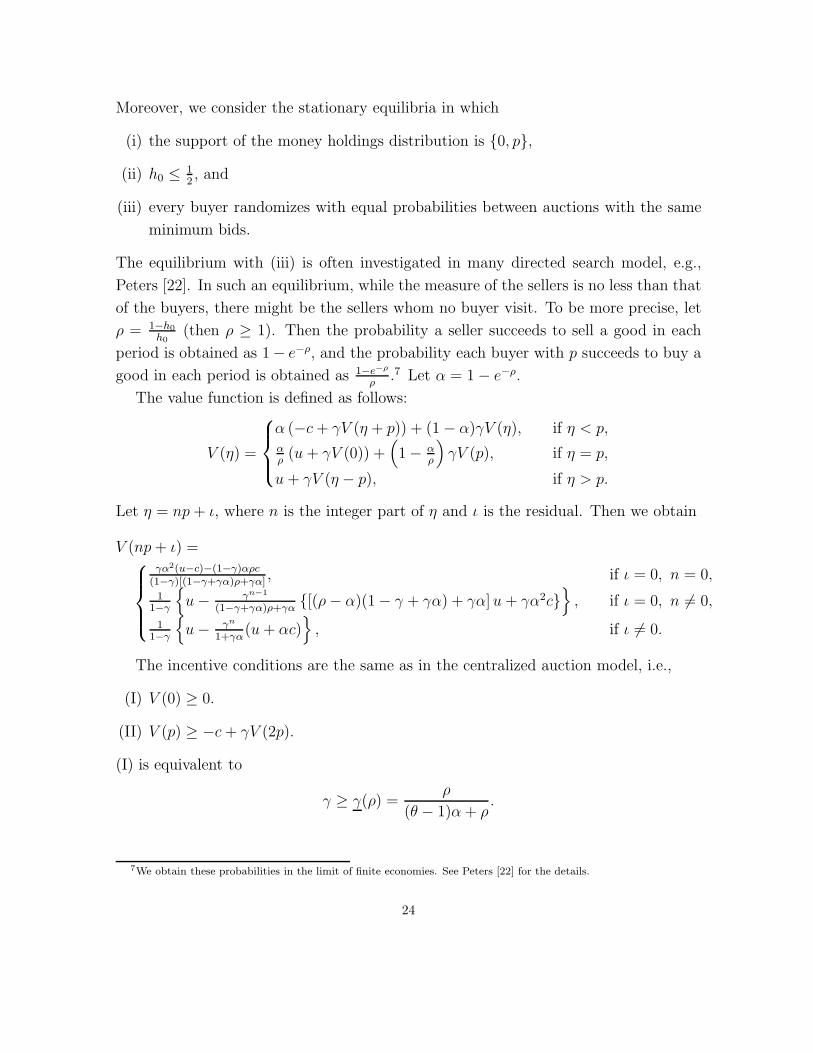
Moreover, we consider the stationary equilibria in which

(i) the support of the money holdings distribution is {0, p},(ii) h0 ≤ 1

2, and

(iii) every buyer randomizes with equal probabilities between auctions with the same

minimum bids.

The equilibrium with (iii) is often investigated in many directed search model, e.g.,

Peters [22]. In such an equilibrium, while the measure of the sellers is no less than that

of the buyers, there might be the sellers whom no buyer visit. To be more precise, let

ρ = 1−h0

h0(then ρ ≥ 1). Then the probability a seller succeeds to sell a good in each

period is obtained as 1− e−ρ, and the probability each buyer with p succeeds to buy a

good in each period is obtained as 1−e−ρ

ρ.7 Let α = 1 − e−ρ.

The value function is defined as follows:

V (η) =

⎧⎪⎨⎪⎩

α (−c + γV (η + p)) + (1 − α)γV (η), if η < p,αρ

(u + γV (0)) +(1 − α

ρ

)γV (p), if η = p,

u + γV (η − p), if η > p.

Let η = np + ι, where n is the integer part of η and ι is the residual. Then we obtain

V (np + ι) =⎧⎪⎪⎨⎪⎪⎩

γα2(u−c)−(1−γ)αρc(1−γ)[(1−γ+γα)ρ+γα]

, if ι = 0, n = 0,

11−γ

{u − γn−1

(1−γ+γα)ρ+γα{[(ρ − α)(1 − γ + γα) + γα]u + γα2c}

}, if ι = 0, n �= 0,

11−γ

{u − γn

1+γα(u + αc)

}, if ι �= 0.

The incentive conditions are the same as in the centralized auction model, i.e.,

(I) V (0) ≥ 0.

(II) V (p) ≥ −c + γV (2p).

(I) is equivalent to

γ ≥ γ(ρ) =ρ

(θ − 1)α + ρ.

7We obtain these probabilities in the limit of finite economies. See Peters [22] for the details.

24

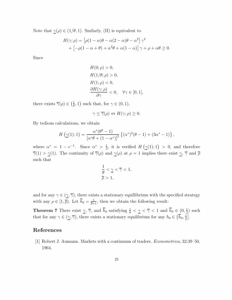
Note that γ(ρ) ∈ (1/θ, 1). Smilarly, (II) is equivalent to

H(γ; ρ) =[ρ(1 − α)θ − α(2 − α)θ − α2

]γ2

+[−ρ(1 − α + θ) + α2θ + α(1 − α)

]γ + ρ + αθ ≥ 0.

Since

H(0; ρ) > 0,

H(1/θ; ρ) > 0,

H(1; ρ) < 0,

∂H(γ; ρ)

∂γ< 0, ∀γ ∈ [0, 1],

there exists γ(ρ) ∈ (1θ, 1

)such that, for γ ∈ (0, 1),

γ ≤ γ(ρ) ⇔ H(γ; ρ) ≥ 0.

By tedious calculations, we obtain

H(γ(1); 1

)=

α∗(θ2 − 1)

[α∗θ + (1 − α∗)]2{(α∗)2(θ − 1) + (3α∗ − 1)

},

where α∗ = 1 − e−1. Since α∗ > 13, it is verified H

(γ(1); 1

)> 0, and therefore

γ(1) > γ(1). The continuity of γ(ρ) and γ(ρ) at ρ = 1 implies there exist γ, γ and ρ

such that

1

θ< γ < γ < 1,

ρ > 1,

and for any γ ∈ (γ, γ), there exists a stationary equillibrium with the specified strategy

with any ρ ∈ [1, ρ). Let h0 = 1ρ+1

, then we obtain the following result:

Theorem 7 There exist γ, γ, and h0 satisfying 1θ

< γ < γ < 1 and h0 ∈ (0, 12) such

that for any γ ∈ (γ, γ), there exists a stationary equilibrium for any h0 ∈(h0,

12

].

References

[1] Robert J. Aumann. Markets with a continuum of traders. Econometrica, 32:39–50,

1964.

25

[2] Gerard Debreu and Herbert E. Scarf. A limit theorem on the core of an economy.

International Economic Review, 3:235–246, 1963.

[3] Pradeep Dubey, Andreu Mas-Colell, and Martin Shubik. Efficiency properties of

strategic market games: An axiomatic approach. Journal of Economic Theory,

22:339–362, 1980.

[4] F. Y. Edgeworth. Mathematical Physics: An Essay on the Application of Mathe-

matics to the Moral Science. Kegan Paul, 1881.

[5] Douglas Gale. Bargaining and competition part i: Characterization. Econometrica,

54(4):785–806, Jul. 1986.

[6] Douglas Gale. Bargaining and competition part ii: Existence. Econometrica,

54(4):807–818, Jul. 1986.

[7] Douglas Gale. Limit theorems for markets with sequential bargaining. Journal of

Economic Theory, 43:20–54, 1987.

[8] Douglas Gale. Strategic Foundations of General Equilibrium: Dynamic Match-

ing and Bargaining Games (Churchill Lectures in Economic Theory). Cambridge

University Press, 2000.

[9] Douglas Gale and Hamid Sabourian. Complexity and competition. Econometrica,

73:739–769, 2005.

[10] Gael Giraud. Strategic market games: an introduction. Journal of Mathematical

Economics, 39:355–375, 2003.

[11] Edward J. Green and Ruilin Zhou. A rudimentary random-matching model with

divisible money and prices. Journal of Economic Theory, 81(2):252–271, 1998.

[12] Edward J. Green and Ruilin Zhou. Dynamic monetary equilibrium in a random

matching economy. Econometrica, 70(3):929–969, 2002.

[13] John R. Hicks. Value and Capital. Clarendon Press, 1939.

[14] Werner Hildenbrand. Core and Equilibria of a Large Economy. Princeton Univer-

sity Press, 1974.

[15] Kazuya Kamiya and Takashi Sato. Equilibrium price dispersion in a matching

model with divisible money. International Economic Review, 45:413–430, 2004.

26

[16] Kazuya Kamiya and Takashi Shimizu. Real indeterminacy of stationary equilibria

in matching models with divisible money. Journal of Mathematical Economics,

forthcoming.

[17] Vijay Krishna. Auction Theory. Academic Press, 2002.

[18] Robert E. Lucas, Jr. Equilibrium in a pure currency economy. Economic Inquiry,

18:203–220, 1980.

[19] Alfred Marshall. Principles of Economics: An Introductory Volume, 8th edn.

Macmillan, 1920.

[20] Akihiko Matsui and Takashi Shimizu. A theory of money and marketplaces. In-

ternational Economic Review, 46:35–59, 2005.

[21] William Novshek and Hugo F. Sonnenshein. Cournot and walras equilibrium.

Journal of Economic Theory, 19:223–266, 1978.

[22] Michael Peters. Ex ante price offers in matching games non-steady states. Econo-

metrica, 59(5):1425–1454, 1991.

[23] Ariel Rubinstein and Asher Wolinsky. Equilibrium in a market with sequential

bargaining. Econometrica, 53(5):1133–1150, Sep. 1985.

[24] Ariel Rubinstein and Asher Wolinsky. Decentralized trading, strategic behaviour

and the walrasian outcome. Review of Economic Studies, 57:63–78, 1990.

[25] Lloyd Shapley and Martin Shubik. Trade using one commodity as a means of

payment. Journal of Political Economy, 85(5):937–968, 1977.

[26] Martin Shubik. Edgeworth market games. In R. Duncan Luce and A. W. Tucker,

editors, Contributioins to the Theory of Games IV. Princeton University Press,

1959.

[27] Nancy L. Stokey, Robert E. Lucas, Jr., and with Edward C. Prescott. Recursive

Methods in Economic Dynamics. Harvard University Press, 1989.

[28] Ruilin Zhou. Individual and aggregate real balances in a random-matching model.

International Economic Review, 40(4):1009–1038, 1999.

27