A Consistent Regularization Approach for

Structured Prediction

Carlo Ciliberto, Alessandro Rudi, Lorenzo Rosasco

University of GenovaIstituto Italiano di Tecnologia - Massachusetts Institute of Technology

lcsl.mit.edu

Dec 9th, NIPS 2016

Structured Prediction

Outline

Standard Supervised Learning

Structured Prediction with SELFAlgorithmTheoryExperiments

Conclusions

Outline

Standard Supervised Learning

Structured Prediction with SELFAlgorithmTheoryExperiments

Conclusions

Scalar Learning

Goal: given (xi, yi)ni=1, find fn : X → Y

Let Y = R

I Parametrize

f(x) = w>ϕ(x) w ∈ RP ϕ : X → RP

I Learn

fn = w>n ϕ(x) wn = argminw∈RP

1

n

n∑i=1

L(w>ϕ(xi), yi)

Multi-variate Learning

Goal: given (xi, yi)ni=1, find fn : X → Y

Let Y = RM

I Parametrize

f(x) = Wϕ(x) W ∈ RM×P ϕ : X → RP

I Learn

fn(x) = Wn ϕ(x) Wn = argminW∈RM×P

1

n

n∑i=1

L(Wϕ(xi), yi)

Learning Theory

Expected Risk

E(f) =

∫X×Y

L(f(x), y) dρ(x, y)

I Consistency

limn→+∞

E(fn) = inffE(f) (in probability)

I Excess Risk Bounds

E(fn)− inff∈H

E(f) . ε(n, ρ,H) (w.h.p.)

Outline

Standard Supervised Learning

Structured Prediction with SELFAlgorithmTheoryExperiments

Conclusions

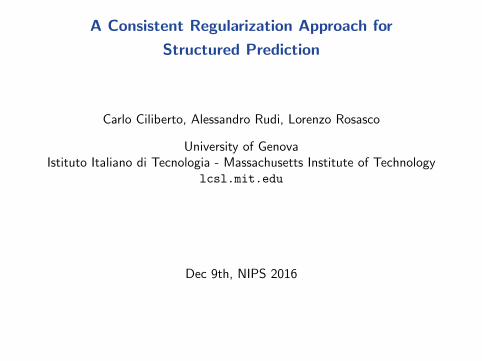
(Un)Structured prediction

What if Y is not a vector space?(e.g. strings, graphs, histograms, etc.)

Q. How do we:

I Parametrize

I Learn

a function f : X → Y ?

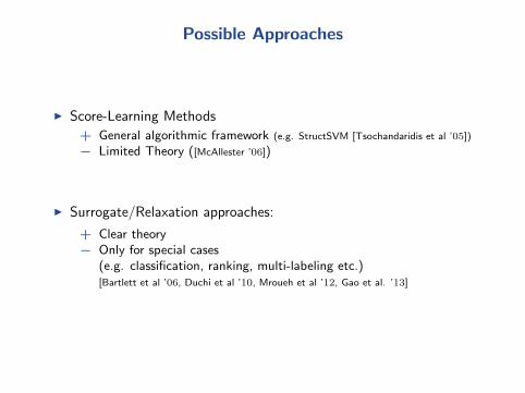
Possible Approaches

I Score-Learning Methods

+ General algorithmic framework (e.g. StructSVM [Tsochandaridis et al ’05])

− Limited Theory ([McAllester ’06])

I Surrogate/Relaxation approaches:

+ Clear theory− Only for special cases

(e.g. classification, ranking, multi-labeling etc.)[Bartlett et al ’06, Duchi et al ’10, Mroueh et al ’12, Gao et al. ’13]

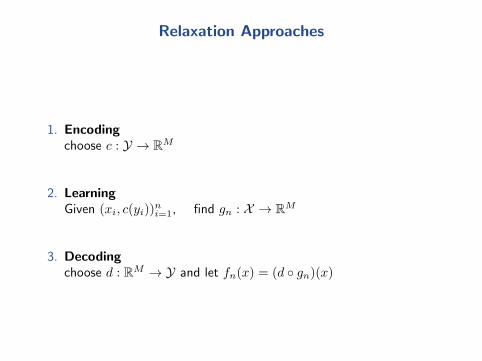
Relaxation Approaches

1. Encodingchoose c : Y → RM

2. LearningGiven (xi, c(yi))

ni=1, find gn : X → RM

3. Decodingchoose d : RM → Y and let fn(x) = (d ◦ gn)(x)

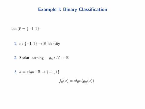
Example I: Binary Classification

Let Y = {−1, 1}

1. c : {−1, 1} → R identity

2. Scalar learning gn : X → R

3. d = sign : R→ {−1, 1}

fn(x) = sign(gn(x))

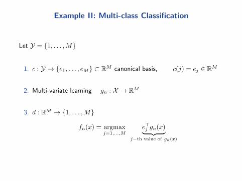
Example II: Multi-class Classification

Let Y = {1, . . . ,M}

1. c : Y → {e1, . . . , eM} ⊂ RM canonical basis, c(j) = ej ∈ RM

2. Multi-variate learning gn : X → RM

3. d : RM → {1, . . . ,M}

fn(x) = argmaxj=1,...,M

e>j gn(x)︸ ︷︷ ︸j−th value of gn(x)

A General Relaxation Approach

Main Assumption. Structure Encoding Loss Function (SELF)

Given 4 : Y × Y → R, there exist:

I HY RKHS with c : Y → HY feature map

I V : HY → HY bounded linear operator

such that:4(y, y′) = 〈c(y), V c(y′)〉HY ∀y, y′ ∈ Y

Note. If V is Positive Semidefinite =⇒ 4 is a kernel.

A General Relaxation Approach

Main Assumption. Structure Encoding Loss Function (SELF)

Given 4 : Y × Y → R, there exist:

I HY RKHS with c : Y → HY feature map

I V : HY → HY bounded linear operator

such that:4(y, y′) = 〈c(y), V c(y′)〉HY ∀y, y′ ∈ Y

Note. If V is Positive Semidefinite =⇒ 4 is a kernel.

SELF: Examples

I Binary classification: c : {−1, 1} → R and V = 1.

I Multi-class classification: c(j) = ej ∈ RM and V = 1− I ∈ RM×M .

I Kernel Dependency Estimation (KDE) [Weston et al. ’02, Cortes et al. ’05]:4(y, y′) = 1− h(y, y′), h : Y × Y → R kernel on Y.

SELF: Finite Y

All 4 on discrete Y are SELF

Examples:

I Strings: edit distance, KL divergence, word error rate, . . .

I Ordered sequences: rank loss, . . .

I Graphs/Trees: graph/trees edit distance, subgraph matching . . .

I Discrete subsets: weighted overlap loss, . . .

I . . .

SELF: More examples

I Histograms/Probabilities: e.g. χ2, Hellinger, . . .

I Manifolds: Diffusion distances

I . . .

Relaxation with SELF

1. Encoding. c : Y → HY canonical feature map of HY

2. Surrogate Learning. Multi-variate regression gn : X → HY

3. Decoding. fn(x) = argminy∈Y

〈c(y), V gn(x)〉HY

Surrogate Learning

Multi-variate learning with ridge regression

I Parametrize

g(x) = Wϕ(x) W ∈ RM×P ϕ : X → RP

I Learn

gn = Wn ϕ(x) Wn = argminW∈RM×P

1

n

n∑i=1

‖Wϕ(xi)− c(yi)‖︸ ︷︷ ︸least-squares

2HY

Learning (cont.)

Solution1

gn(x) = Wn ϕ(x)

Wn = C (Φ>Φ)−1Φ>︸ ︷︷ ︸A∈Rn×n

= CA

I Φ = [ϕ(x1), . . . , ϕ(xn)] ∈ RP×n input features

I C = [c(y1), . . . , c(yn)] ∈ RM×n output features

1In practice add a regularizer!

Decoding

Lemma (Ciliberto, Rudi, Rosasco ’16)

Let gn(x) = CA ϕ(x) solution the surrogate problem. Then

fn(x) = argminy∈Y

〈c(y), V gn(x)〉HY

can be written as

fn(x) = argminy∈Y

n∑i=1

αi(x)4 (y, yi)

where(α1(x), . . . , αn(x))> = A ϕ(x) ∈ Rn

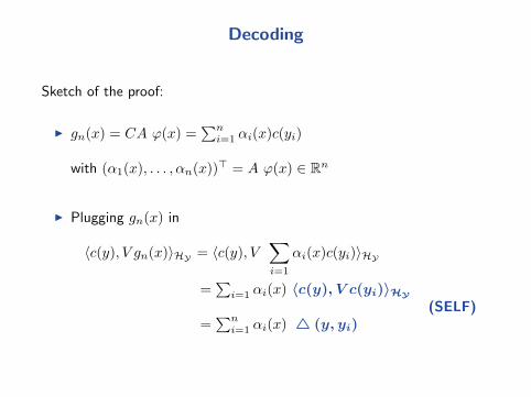
Decoding

Sketch of the proof:

I gn(x) = CA ϕ(x) =∑n

i=1 αi(x)c(yi)

with (α1(x), . . . , αn(x))> = A ϕ(x) ∈ Rn

I Plugging gn(x) in

〈c(y), V gn(x)〉HY = 〈c(y), V∑i=1

αi(x)c(yi)〉HY

=∑

i=1 αi(x) 〈c(y), V c(yi)〉HY

=∑n

i=1 αi(x) 4 (y, yi)(SELF)

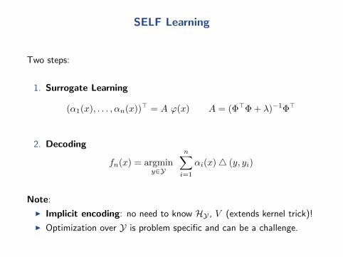
SELF Learning

Two steps:

1. Surrogate Learning

(α1(x), . . . , αn(x))> = A ϕ(x) A = (Φ>Φ + λ)−1Φ>

2. Decoding

fn(x) = argminy∈Y

n∑i=1

αi(x)4 (y, yi)

Note:

I Implicit encoding: no need to know HY , V (extends kernel trick)!

I Optimization over Y is problem specific and can be a challenge.

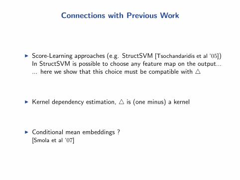
Connections with Previous Work

I Score-Learning approaches (e.g. StructSVM [Tsochandaridis et al ’05])In StructSVM is possible to choose any feature map on the output...... here we show that this choice must be compatible with 4

I Kernel dependency estimation, 4 is (one minus) a kernel

I Conditional mean embeddings ?[Smola et al ’07]

Relaxation Analysis

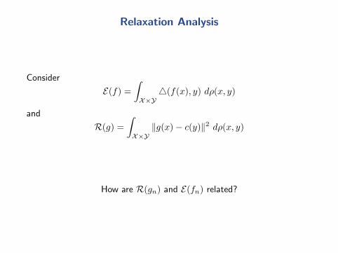
Consider

E(f) =

∫X×Y

4(f(x), y) dρ(x, y)

and

R(g) =

∫X×Y

‖g(x)− c(y)‖2 dρ(x, y)

How are R(gn) and E(fn) related?

Relaxation Analysis

Consider

E(f) =

∫X×Y

4(f(x), y) dρ(x, y)

and

R(g) =

∫X×Y

‖g(x)− c(y)‖2 dρ(x, y)

How are R(gn) and E(fn) related?

Relaxation Analysis

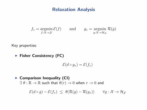
f∗ = argminf :X→Y

E(f) and g∗ = argming:X→HY

R(g)

Key properties:

I Fisher Consistency (FC)

E(d ◦ g∗) = E(f∗)

I Comparison Inequality (CI)∃ θ : R→ R such that θ(r)→ 0 when r → 0 and

E(d ◦ g)− E(f∗) ≤ θ(R(g)−R(g∗)) ∀g : X → HY

SELF Relaxation Analysis

Theorem (Ciliberto, Rudi, Rosasco ’16)

4 : Y ×Y → R SELF loss, g∗ : X → HY least-square “relaxed” solution.

Then

I Fisher ConsistencyE(d ◦ g∗) = E(f∗)

I Comparison Inequality ∀g : X → HY

E(d ◦ g)− E(f∗) .√R(g)−R(g∗)

SELF Relaxation Analysis (cont.)

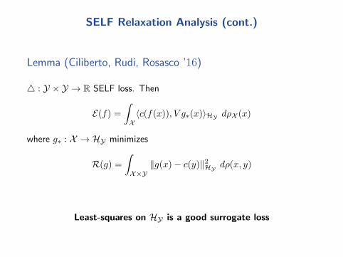
Lemma (Ciliberto, Rudi, Rosasco ’16)

4 : Y × Y → R SELF loss. Then

E(f) =

∫X〈c(f(x)), V g∗(x)〉HY dρX (x)

where g∗ : X → HY minimizes

R(g) =

∫X×Y

‖g(x)− c(y)‖2HY dρ(x, y)

Least-squares on HY is a good surrogate loss

Consistency and Generalization Bounds

Theorem (Ciliberto, Rudi, Rosasco ’16)If we consider a universal feature map and λ = 1/

√n, then,

limn→∞

E(fn) = E(f∗), almost surely

Moreover, under mild assumptions

E(fn)− E(f∗) . n−1/4 (w.h.p.)

Proof.Relaxation analysis + (kernel) ridge regression results

R(gn)−R(g∗) . n−1/2

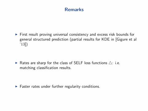
Remarks

I First result proving universal consistency and excess risk bounds forgeneral structured prediction (partial results for KDE in [Gigure et al’13])

I Rates are sharp for the class of SELF loss functions 4: i.e.matching classification results.

I Faster rates under further regularity conditions.

Experiments: Ranking

4rank(f(x), y) =

M∑i,j=1

γ(y)ij (1− sign(f(x)i − f(x)j))/2

Rank Loss

[Herbrich et al. ’99] 0.432± 0.008[Dekel et al. ’04] 0.432± 0.012[Duchi et al. ’10] 0.430± 0.004

[Tsochantaridis et al. ’05] 0.451± 0.008[Ciliberto, Rudi, R. ’16] 0.396± 0.003

Ranking experiments on the MovieLens dataset with 4rank [Dekel et al. ’04,

Duchi et al. ’10]. ∼ 1600 Movies for ∼ 900 users.

Experiments: Digit Reconstruction

Digit reconstruction on USPS dataset

Loss KDE SELF4G 4H

4G 0.149± 0.013 0.172± 0.0114H 0.736± 0.032 0.647± 0.0174R 0.294± 0.012 0.193± 0.015

I 4G(f(x), y) = 1− k(f(x), y) k Gaussian kernel on the output.

I 4H(f(x), y) = ‖√f(x)−√y‖ Hellinger distance.

I 4R(f(x), y) Recognition accuracy of an SVM digit classifier.

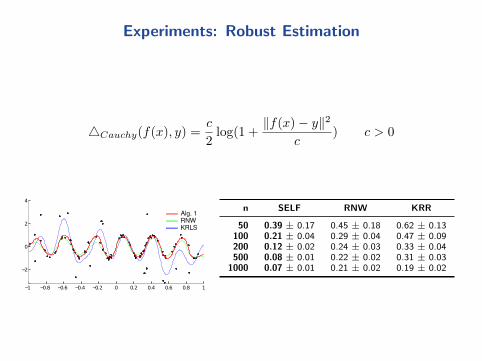
Experiments: Robust Estimation

4Cauchy(f(x), y) =c

2log(1 +

‖f(x)− y‖2

c) c > 0

−1 −0.8 −0.6 −0.4 −0.2 0 0.2 0.4 0.6 0.8 1

−2

0

2

4

Alg. 1RNWKRLS

n SELF RNW KRR

50 0.39 ± 0.17 0.45 ± 0.18 0.62 ± 0.13100 0.21 ± 0.04 0.29 ± 0.04 0.47 ± 0.09200 0.12 ± 0.02 0.24 ± 0.03 0.33 ± 0.04500 0.08 ± 0.01 0.22 ± 0.02 0.31 ± 0.03

1000 0.07 ± 0.01 0.21 ± 0.02 0.19 ± 0.02

Outline

Standard Supervised Learning

Structured Prediction with SELFAlgorithmTheoryExperiments

Conclusions

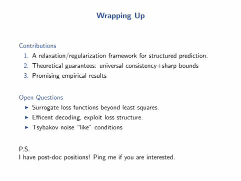
Wrapping Up

Contributions

1. A relaxation/regularization framework for structured prediction.

2. Theoretical guarantees: universal consistency+sharp bounds

3. Promising empirical results

Open Questions

I Surrogate loss functions beyond least-squares.

I Efficent decoding, exploit loss structure.

I Tsybakov noise “like” conditions

P.S.I have post-doc positions! Ping me if you are interested.