A Combinatorial Data Analysis Toolbox for MATLABcda.psych.uiuc.edu/cdatool/cdatoolr1.pdf · others....

A Combinatorial Data AnalysisToolbox for MATLAB

The HAM Team

October 7, 2002

Contents

I Linear Unidimensional Scaling (LUS) 2

1 LUS in the L2 Norm 5

1.1 Optimization Methods for∑

i(t(ρ)i )2 . . . . . . . . . . 6

1.1.1 Dynamic Programming . . . . . . . . . . . . 7

1.1.2 Iterative Quadratic Assignment . . . . . . . . 11

1.1.3 Gradient-Based Optimization . . . . . . . . . 21

1.1.4 A Nonlinear Programming Heuristic . . . . . . 24

1.1.5 Solving Linear (In)equality Constrained Least

Squares Tasks:

The Example of the Confirmatory Fitting of a

Given Order . . . . . . . . . . . . . . . . . . 28

1.1.6 Some Useful Utilities for Transforming and Dis-

playing Proximity Matrices . . . . . . . . . . 32

1.2 The Incorporation of Additive Constants in L2 LUS . 41

1.2.1 The L2 Fitting of a Single Unidimensional Scale

(with an Additive Constant) . . . . . . . . . . 43

1.2.2 The L2 Finding and Fitting of Multiple Unidi-

mensional Scales . . . . . . . . . . . . . . . . 49

1

1.2.3 Incorporating Monotonic Transformation of a

Proximity Matrix in Fitting Multiple Unidi-

mensional Scales: L2 Nonmetric Multidimen-

sional Scaling in the City-Block Metric . . . . 54

2 LUS in the L1 Norm 59

2.1 The L1 Fitting of a Single Unidimensional Scale . . . 60

2.1.1 Iterative Linear Programming . . . . . . . . . 64

2.2 The L1 Finding and Fitting of Multiple Unidimen-

sional Scales . . . . . . . . . . . . . . . . . . . . . . 67

A main program files 74

A.1 uniscaldp.m . . . . . . . . . . . . . . . . . . . . . . 74

A.2 uniscaldpf.m . . . . . . . . . . . . . . . . . . . . . . 78

A.2.1 uscalfor.for . . . . . . . . . . . . . . . . . . . 79

A.2.2 uscalforgw.for . . . . . . . . . . . . . . . . . . 82

A.3 uniscalqa.m . . . . . . . . . . . . . . . . . . . . . . . 83

A.4 guttorder.m . . . . . . . . . . . . . . . . . . . . . . 87

A.5 plinorder.m . . . . . . . . . . . . . . . . . . . . . . . 89

A.6 unifitl2nlp.m . . . . . . . . . . . . . . . . . . . . . . 92

A.6.1 objfunl2.m . . . . . . . . . . . . . . . . . . . 95

A.7 linfit.m . . . . . . . . . . . . . . . . . . . . . . . . . 96

A.8 linfitac.m . . . . . . . . . . . . . . . . . . . . . . . . 99

A.9 biscalqa.m . . . . . . . . . . . . . . . . . . . . . . . 102

A.10 triscalqa.m . . . . . . . . . . . . . . . . . . . . . . . 110

A.11 bimonscalqa.m . . . . . . . . . . . . . . . . . . . . . 122

A.12 trimonscalqa.m . . . . . . . . . . . . . . . . . . . . . 124

A.13 linfitl1.m . . . . . . . . . . . . . . . . . . . . . . . . 126

2

A.14 linfitl1ac.m . . . . . . . . . . . . . . . . . . . . . . . 128

A.15 uniscallp.m . . . . . . . . . . . . . . . . . . . . . . . 131

A.16 uniscallpac.m . . . . . . . . . . . . . . . . . . . . . . 132

A.17 biscallp.m . . . . . . . . . . . . . . . . . . . . . . . 133

B utility program files 138

B.1 ransymat.m . . . . . . . . . . . . . . . . . . . . . . 138

B.2 A GAUSS procedure corresponding to uniscaldp.m . . 139

B.3 Iterative improvement Quadratic Assignment proce-

dures . . . . . . . . . . . . . . . . . . . . . . . . . . 142

B.3.1 pairwiseqa.m . . . . . . . . . . . . . . . . . . 142

B.3.2 rotateqa.m . . . . . . . . . . . . . . . . . . . 143

B.3.3 insertqa.m . . . . . . . . . . . . . . . . . . . 145

B.4 proxstd.m . . . . . . . . . . . . . . . . . . . . . . . 147

B.5 proxrand.m . . . . . . . . . . . . . . . . . . . . . . . 148

B.6 proxmon.m . . . . . . . . . . . . . . . . . . . . . . . 148

B.7 matcolor.m . . . . . . . . . . . . . . . . . . . . . . . 152

3

Part I

Linear Unidimensional Scaling (LUS)

4

The task of linear unidimensional scaling (LUS) can be characterized as a very specificdata analysis problem: given a set of n objects, S = O1, ..., On, and an n × n symmetricproximity matrix P = pij, arrange the objects along a single dimension such that the in-duced n(n− 1)/2 interpoint distances between the objects reflect the proximities in P. Theterm “proximity” merely refers to some arbitrary symmetric numerical measure of relation-ship between each object pair (pij = pji for 1 ≤ i, j ≤ n) and for which all self-proximitiesare considered irrelevant and set equal to zero (pii = 0 for 1 ≤ i ≤ n). As a technical con-venience, proximities are assumed nonnegative and are given a dissimilarity interpretation,i.e., large proximities refer to dissimilar objects.

Given the inherent vagueness regarding the technical details involved in the unidimen-sional scaling task, it should not be surprising that a variety of approaches to it are availablein the literature. As a starting point to be developed first in Chapter 1, we consider anobvious formalization assuming the interpoint distances along a continuum are Euclideanand that the measure of how close the interpoint distances are to the given proximities is thesum of squared discrepancies. Specifically, we wish to find the n coordinates, x1, x2, . . . , xn,such that the least-squares (or L2) criterion∑

i<j

(pij − |xj − xi|)2 (1)

is minimized. Although there is some inherent arbitrariness in the selection of this measureof goodness-of-fit for metric scaling and the reliance on Euclidean interpoint distances, thesechoices are traditional and have been discussed in some detail in the literature by Guttman(1968), Defays (1978), de Leeuw and Heiser (1977), and Hubert and Arabie (1986), amongothers. In the first chapter that follows in this Part I, we present several functions in theCombinatorial Data Analysis (CDA) Toolbox (within a MATLAB environment) for this L2

task based on a number of different optimization strategies, e.g., dynamic programming, theiterative use of a quadratic assignment improvement heuristic, Pliner’s technique of smooth-ing, the original Guttman update method, and a nonlinear programming reformulation byLau, Leung, and Tse (1998). Several generalizations of the unidimensional scaling task aregiven (along with appropriate Toolbox implementations): the incorporation of a fitted ad-ditive constant by replacing the absolute coordinate difference |xj − xi| by [|xj − xi| − c],where c is a constant to be estimated along with the n coordinates; the extension to multiple(additive) unidimensional scalings of a common proximity matrix; and in Chapter 2, thereplacement of the L2 least-squares loss function by the minimization of the sum of absolutedeviations (the L1 criterion).

In addition to making available the basic MATLAB m-functions for carrying out thevarious unidimensional scaling tasks, several important computational improvements arealso discussed and compared. These involve either transforming a given m-function withthe MATLAB Compiler into C code that can in turn be submitted to a C/C++ compiler,or alternatively, rewriting an m-function and the mandatory MATLAB gateway directly inFortran90 and then compiling into a MATLAB callable *.dll file (within a windows envi-ronment). In some cases studied, the computational improvements are very dramatic when

5

the use of an external Fortran coded *.dll is compared either to one generated through Cby use of the MATLAB Compiler, or as might be more expected, to the original interpretedm-function directly within a MATLAB environment.

6

Chapter 1

LUS in the L2 Norm

As an alternative reformulation of the L2 unidimensional scaling task that will prove veryconvenient as a point of departure in our development of computational routines, the op-timization suggested by (1) can be subdivided into two separate problems to be solvedsimultaneously: find a set of n numbers, x1 ≤ x2 ≤ · · · ≤ xn, and a permutation on the firstn integers, ρ(·) ≡ ρ, for which ∑

i<j

(pρ(i)ρ(j) − (xj − xi))2 (1.1)

is minimized. Thus, a set of locations (coordinates) is defined along a continuum as repre-sented in ascending order by the sequence x1, x2, . . . , xn; the n objects are allocated to theselocations by the permutation ρ, i.e., object Oρ(i) is placed at location i. In fact, without lossof generality we can and will impose one additional constraint that

∑i xi = 0, i.e., any set of

values, x1, x2, . . . , xn, can be replaced by x1 − x, x2 − x, . . . , xn − x, where x = (1/n)∑

i xi,without altering the value of (1) or (1.1). Formally, if ρ∗ and x∗1 ≤ x∗2 ≤ · · · ≤ x∗n define aglobal minimum of (1.1), and Ω denotes the set of all permutations of the first n integers,then ∑

i<j

(pρ∗(i)ρ∗(j) − (x∗j − x∗i ))2 =

min[∑i<j

(pρ(i)ρ(j) − (xj − xi))2 | ρ ∈ Ω; x1 ≤ · · · ≤ xn;

∑i

xi = 0].

The measure of loss in (1.1) can be reduced algebraically:∑i<j

p2ij + n(

∑i

x2i − 2

∑i

xit(ρ)i ), (1.2)

subject to the constraints that x1 ≤ · · · ≤ xn and∑

i xi = 0, and letting

t(ρ)i = (u

(ρ)i − v

(ρ)i )/n,

where

u(ρ)i =

i−1∑j=1

pρ(i)ρ(j) for i ≥ 2;

7

v(ρ)i =

n∑j=i+1

pρ(i)ρ(j) for i < n,

andu

(ρ)1 = v(ρ)

n = 0.

In words, u(ρ)i is the sum of the entries within row ρ(i) of pρ(i)ρ(j) from the extreme left up

to the main diagonal; v(ρ)i is the sum from the main diagonal to the extreme right. Or, we

might rewrite (1.2) as

∑i<j

p2ij + n

(∑i

(xi − t(ρ)i )2 −

∑i

(t(ρ)i )2

). (1.3)

In (1.3), the two terms∑

i(xi − t(ρ)i )2 and

∑i(t

(ρ)i )2 control the size of the discrepancy index

since∑

i<j p2ij is constant for any given data matrix. Thus, to minimize the original index in

(1.1), we should simultaneously minimize∑

i(xi− t(ρ)i )2 and maximize

∑i(t

(ρ)i )2. If the equiv-

alent form of (1.2) is considered, our concern would be in minimizing∑

i x2i and maximizing∑

i xit(ρ)i .

As noted first by Defays (1978), the minimization of (1.3) can be carried out directly

by the maximization of the single term,∑

i(t(ρ)i )2 (under the mild regularity condition that

all off-diagonal proximities in P are positive and not merely nonnegative). Explicitly, if

ρ∗ is a permutation that maximizes∑

i(t(ρ)i )2, then we can let xi = t

(ρ∗)i , which eliminates

the term∑

i(xi − t(ρ∗)i )2 from (1.3). In short, because the order induced by t

(ρ∗)1 , . . . , t(ρ

∗)n is

consistent with the constraint x1 ≤ x2 ≤ · · · ≤ xn, the minimization of (1.3) reduces to the

maximization of the single term∑

i(t(ρ)i )2 with the coordinate estimation completed as an

automatic byproduct.

1.1 Optimization Methods for∑

i(t(ρ)i )2

The maximization of∑

i(t(ρ)i )2 over all permutations is a prototypical combinatorial optimiza-

tion task, and a variety of different methods are available for its solution. Unfortunately,because this optimization task is representative of the class of so-called NP-hard problems(e.g., see Garey and Johnson, 1979), any procedure yielding verifiably globally optimal so-lutions would be severely limited by the size of the matrices that could be realisticallyprocessed. We begin in the first subsection below, the discussion of a dynamic programmingstrategy for the maximization of

∑i(t

(ρ)i )2 proposed by Hubert and Arabie (1986) that will

produce globally optimal solutions for proximity matrices of sizes up to, say, the low twenties(within a MATLAB environment). We will provide and illustrate in some detail a MAT-LAB function that carries out the optimization; also as a mechanism for speeding up theoptimization, we discuss the use of the MATLAB C/C++ Compiler and external Fortransubroutines and their gateways to allow externally generated functions to be callable fromMATLAB. The other subsections of this section present other (heuristic) methods for the

8

maximization of∑

i(t(ρ)i )2 and illustrate the use of their MATLAB function implementations

that are provided.It is convenient to have a small numerical example available as we discuss the various

optimization strategies in the unidimensional scaling context. To this end we list a datafile below, called ‘number.dat’, that contains a dissimilarity matrix taken from Shepard,Kilpatric, and Cunningham (1975). The stimulus domain is the first ten single-digits 0,1,2,. . . , 9 considered as abstract concepts; the 10 × 10 proximity matrix (with an ith row orcolumn corresponding to the i− 1 digit) was constructed by averaging dissimilarity ratingsfor distinct pairs of those integers over a number of subjects and conditions. An inspection ofthese data suggests there may be some very regular but possibly complex manifest patterningreflecting either structural characteristics of the digits (e.g., the powers of 2 or of 3, thesalience of the two additive/multiplicative identities [0/1], oddness/evenness), or of absolutemagnitudes. These data will be relied on to provide concrete numerical illustrations of thevarious MATLAB functions we introduce, and will be loaded as a proximity matrix (andimportantly, as one that is symmetric and has zero values along the main diagonal) in theMATLAB environment by the command ‘load number.dat’.

.000 .421 .584 .709 .684 .804 .788 .909 .821 .850

.421 .000 .284 .346 .646 .588 .758 .630 .791 .625

.584 .284 .000 .354 .059 .671 .421 .796 .367 .808

.709 .346 .354 .000 .413 .429 .300 .592 .804 .263

.684 .646 .059 .413 .000 .409 .388 .742 .246 .683

.804 .588 .671 .429 .409 .000 .396 .400 .671 .592

.788 .758 .421 .300 .388 .396 .000 .417 .350 .296

.909 .630 .796 .592 .742 .400 .417 .000 .400 .459

.821 .791 .367 .804 .246 .671 .350 .400 .000 .392

.850 .625 .808 .263 .683 .592 .296 .459 .392 .000

1.1.1 Dynamic Programming

To maximize∑

i(t(ρ)i )2 over all permutations, we construct a function, F(·), by recursion for

all possible subsets of the first n integers, 1, 2, . . . , n:a) F() = 0, where is the empty set;

b) F(R′) = max[F(R) + d(R, i)], where R′ and R are subsets of size k + 1 and k,respectively; the maximum is taken over all subsets R and indices i such that R′ = R ∪ i;and d(R, i) is the incremental value that would be added to the criterion if the objects in Rhad formed the first k values assigned by the optimal permutation and i had been the nextassignment made, i.e., ρ(k + 1) = i. Explicitly,

d(R, i) = [(1/n)∑j∈R

pij −∑

j( 6=i)/∈R

pij]2;

c) the optimal value of the criterion, i.e., F(1, 2, . . . , n), is obtained for R = 1, 2, . . . , nand the optimal permutation, ρ∗, identified by working backwards through the recursion to

9

identify the sequence of successive subsets of decreasing size that led to the value attainedfor F(1, 2, . . . , n).

This type of dynamic programming strategy is a very general one and can be used for anycriterion for which the incremental value in identifying the index to be assigned to ρ(k + 1)does not depend on the particular order of the assigned values in the set ρ(1), . . . , ρ(k).The reader might refer to Hubert, Arabie, and Meulman (2001) for many more applicationsof dynamic programming in the combinatorial data analysis context.

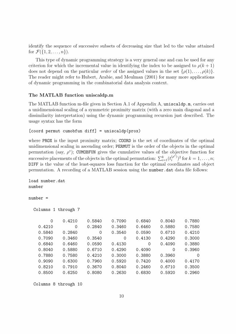
The MATLAB function uniscaldp.m

The MATLAB function m-file given in Section A.1 of Appendix A, uniscaldp.m, carries outa unidimensional scaling of a symmetric proximity matrix (with a zero main diagonal and adissimilarity interpretation) using the dynamic programming recursion just described. Theusage syntax has the form

[coord permut cumobfun diff] = uniscaldp(prox)

where PROX is the input proximity matrix; COORD is the set of coordinates of the optimalunidimensional scaling in ascending order; PERMUT is the order of the objects in the optimalpermutation (say, ρ∗); CUMOBFUN gives the cumulative values of the objective function for

successive placements of the objects in the optimal permutation:∑k

i=1(t(ρ∗)i )2 for k = 1, . . . , n;

DIFF is the value of the least-squares loss function for the optimal coordinates and objectpermutation. A recording of a MATLAB session using the number.dat data file follows:

load number.dat

number

number =

Columns 1 through 7

0 0.4210 0.5840 0.7090 0.6840 0.8040 0.7880

0.4210 0 0.2840 0.3460 0.6460 0.5880 0.7580

0.5840 0.2840 0 0.3540 0.0590 0.6710 0.4210

0.7090 0.3460 0.3540 0 0.4130 0.4290 0.3000

0.6840 0.6460 0.0590 0.4130 0 0.4090 0.3880

0.8040 0.5880 0.6710 0.4290 0.4090 0 0.3960

0.7880 0.7580 0.4210 0.3000 0.3880 0.3960 0

0.9090 0.6300 0.7960 0.5920 0.7420 0.4000 0.4170

0.8210 0.7910 0.3670 0.8040 0.2460 0.6710 0.3500

0.8500 0.6250 0.8080 0.2630 0.6830 0.5920 0.2960

Columns 8 through 10

10

0.9090 0.8210 0.8500

0.6300 0.7910 0.6250

0.7960 0.3670 0.8080

0.5920 0.8040 0.2630

0.7420 0.2460 0.6830

0.4000 0.6710 0.5920

0.4170 0.3500 0.2960

0 0.4000 0.4590

0.4000 0 0.3920

0.4590 0.3920 0

[coord permut cumobfun diff] = uniscaldp(number)

coord =

-0.6570

-0.4247

-0.2608

-0.1492

-0.0566

0.0842

0.1988

0.3258

0.4050

0.5345

permut =

1

2

3

5

4

6

7

9

10

8

11

cumobfun =

43.1649

61.2019

68.0036

70.2296

70.5500

71.2590

75.2111

85.8257

102.2282

130.7972

diff =

1.9599

The second column of Table 1.1 provides some time comparisons (in seconds) for theuse of uniscaldp.m over randomly constructed proximity matrices of size n × n for n =10 to 24. The matrices were randomly generated using the utility program ransymat.m

given in Section B.1 of Appendix B (the usage syntax of ransymat.m can be seen from itsheader comments). The computer on which these times were obtained is a laptop with a750MHz Pentium processor and 512MB of RAM; for matrices of size 25 × 25 and above,an “insufficient memory” message is obtained so the largest matrix size possible in Table1.1 is 24. The execution times (obtained using the tic toc command pair in MATLAB)range from 1.43 seconds for n = 10 to a rather enormous 116550.0 seconds for n = 24(which is about 32.4 hours). As can be seen from the timings given, there is a fairly regularproportional increase in execution time of about 2.2 for each unit increase in n.

The MATLAB C/C++ Compiler

One of the separate add-on components that can be obtained with MATLAB is a C/C++Compiler that when applied to a function m-file, such as uniscaldp.m, produces C or C++code. The latter can itself then be compiled by a separate C/C++ compiler to produce(in a windows environment) a *.dll file that can be called within MATLAB just like a *.mfunction. As an example, we first renamed a version of uniscaldp.m to uniscaldpc.m

and then applied in MATLAB 6 the C/C++ Compiler Version 2.1 with all the possibleoptimization options selected; the resulting code was compiled with the built-in C compiler(called lcc) to produce uniscaldpc.dll

We give the timings for the use of uniscaldpc.dll in the third column of Table 1.1. Asn increases by 1, the execution times increase by about 2.2 just as for uniscaldp.m; but

12

overall, the compiled uniscaldpc.dll executes at about 4.3 times faster than the interpretedfile uniscaldp.m.

A GAUSS procedure paralleling uniscaldp.m

One of the arguments heard informally (at least among some of our colleagues) for usingthe program GAUSS rather than MATLAB is that the former is generally much faster com-putationally than the latter, even though both are interpreters. To evaluate this conjecturewithin the present unidimensional scaling context, a GAUSS procedure, given in AppendixB.2, was written that parallels uniscaldp.m. The fourth column of Table 1.1 gives the tim-ings for the recent version of GAUSS (Version 3.5). Again, there is an increase in executiontime of about 2.2 for each unit increase in n; GAUSS, however, is about 7.5 times fasterthan the comparable MATLAB function, and even about 1.8 times faster than using the Ccompiled uniscaldpc.dll. Our colleagues apparently have a point here.

External Fortran subroutines

One strategy for decreasing the execution time of an m-file would replace part of the code thatmay be slow (usually nonvectorizable “for” loops, for example) by a call to a *.dll that is pro-duced from a Fortran subroutine implementing the code in its own language. As an example,the m-function listed in Appendix A.2, uniscaldpf.m, is a parallel of uniscaldp.m exceptthat the actual recursion constructing the two crucial vectors (and from which the optimalsolution is eventually identified by working backwards) is replaced by a call to uscalfor.dll.This latter file (called a Fortran MEX-file in MATLAB) was produced using the MATLABApplication Program Interface (API) through the Digital Visual Fortran90 (6.0) Compilerand with the central computational Fortran subroutine uscalfor.for in Appendix SectionA.2.1 and the second necessary gateway Fortran subroutine uscalforgw.for in AppendixSection A.2.2. These two subroutines are compiled together to produce uscalfor.dll thatis then called in uniscaldpf.m to do “the heavy lifting”.

In comparison to the other times listed in Table 1.1, the speedup provided by usingthe routine uniscaldpf.m is rather incredible. There is generally the same type of 2.2proportional increase in time for each unit change in n (except for the odd anomaly forn = 24, which must be due to some type of caching/virtual memory difficulty). In comparisonto the basic m-function, uniscaldp.m, there is a 700/800 increase in speed for uniscaldpf.m.As one dramatic example, when n = 23 the analysis takes about a minute for uniscaldpf.m,but 15.5 hours for uniscaldp.m.

1.1.2 Iterative Quadratic Assignment

Because of the manner in which the discrepancy index for the unidimensional scaling taskcan be rephrased as in (1.2) and (1.3), the two optimization subproblems to be solved simul-taneously of identifying an optimal permutation and a set of coordinates can be separated:

13

Table 1.1: Time comparisons in seconds for the various implementations of unidimensionalscaling through dynamic programming

matrix size uniscaldp.m uniscaldpc.dll gauss/uniscaldp uniscaldpf.m10 1.43 .33 .22 .0011 3.30 .77 .44 .0012 7.42 1.81 .99 .0013 16.75 3.96 2.25 .0014 37.62 8.90 5.05 .0515 83.98 19.88 11.37 .1716 186.09 43.99 25.54 .2817 411.45 96.95 56.63 .6018 904.57 212.56 125.01 1.4319 2007.5 465.66 272.65 3.0220 4465.4 1050.3 595.29 6.5421 11415. 2236.9 1351.3 14.0622 24728. 4992.4 3103.8 30.0423 55706. 12451. 6840.5 63.8824 116550. 23371. 15942. 1148.4

(a) assuming that an ordering of the objects is known (and denoted, say, as ρ0 for the

moment), find those values x01 ≤ · · · ≤ x0

n to minimize∑

i(x0i − t

(ρ0)i )2. If the permutation ρ0

produces a monotonic form for the matrix pρ0(i)ρ0(j) in the sense that t(ρ0)1 ≤ t

(ρ0)2 ≤ · · · ≤

t(ρ0)

n , the coordinate estimation is immediate by letting x0i = t

(ρ0)i , in which case

∑i(x

0i−t

(ρ0)i )2

is zero.

(b) assuming that the locations x01 ≤ · · · ≤ x0

n are known, find the permutation ρ0

to maximize∑

i xit(ρ0)i . We note from the work of Hubert and Arabie (1986, p. 189) that

any such permutation which even only locally maximizes∑

i xit(ρ0)i in the sense that no

adjacently placed pair of objects in ρ0 could be interchanged to increase the index, willproduce a monotonic form for the non-negative matrix pρ0(i)ρ0(j). Also, the task of finding

the permutation ρ0 to maximize∑

i xit(ρ0)i is actually a quadratic assignment (QA) task which

has been discussed extensively in the literature of operations research, e.g., see Francis andWhite (1974), Lawler (1975), Hubert and Schultz (1976), among others. As usually defined, aQA problem involves two n×n matrices A = aij and B = bij, and we seek a permutationρ to maximize

Γ(ρ) =∑i,j

aρ(i)ρ(j)bij. (1.4)

If we define bij = |xi − xj| and let aij = pij, then

Γ(ρ) =∑i,j

pρ(i)ρ(j)|xi − xj| = 2n∑

i

xit(ρ)i ,

14

and thus, the permutation that maximizes Γ(ρ) also maximizes∑

xit(ρ)i .

The QA optimization task as formulated through (1.4) has an enormous literature at-tached to it, and the reader is referred to Pardalos and Wolkowicz (1994) for an up-to-dateand comprehensive review. For current purposes and as provided in three general m-functionsof the next subsection (pairwiseqa.m, rotateqa.m, and insertqa.m), one might considerthe optimization of (1.4) through simple object interchange/rearrangement heuristics. Basedon given matrices A and B, and beginning with some permutation (possibly chosen at ran-dom), local interchanges/rearrangements of a particular type are implemented until no im-provement in the index can be made. By repeatedly initializing such a process randomly, adistribution over a set of local optima can be achieved. At least within the context of somecommon data analysis applications, such a distribution may be highly relevant diagnosticallyfor explaining whatever structure might be inherent in the matrix A.

In a subsequent subsection below, we introduce the main m-function (uniscalqa.m) forunidimensional scaling based on these earlier QA optimization strategies. In effect, we beginwith an equally-spaced set of fixed coordinates with their interpoint distances defining the Bmatrix of the general QA index in (1.4) and a random object permutation; a locally-optimalpermutation is then identified through a collection of local interchanges/rearrangements; thecoordinates are re-estimated based on this identified permutation, and the whole processrepeated until no change can be made in either the identified permutation or coordinatecollection.

The QA interchange/rearrangement heuristics

The three m-functions of Appendix B.3 that carry out general QA interchange/rearrangementheuristics all have the same general usage syntax:

[outperm rawindex allperms index] = pairwiseqa(prox,targ,inperm)

[outperm rawindex allperms index] = rotateqa(prox,targ,inperm,kblock)

[outperm rawindex allperms index] = insertqa(prox,targ,inperm,kblock)

pairwiseqa.m carries out an iterative QA maximization task using the pairwise interchangesof objects in the current permutation defining the row and column order of the data ma-trix. All possible such interchanges are generated and considered in turn, and whenever anincrease in the cross-product index would result from a particular interchange, it is madeimmediately. The process continues until the current permutation cannot be improved uponby any such pairwise object interchange; this final locally optimal permutation is OUTPERM

The input beginning permutation is INPERM (a permutation of the first n integers); PROX

is the n × n input proximity matrix and TARG is the n × n input target matrix (which arerespective analogues of the matrices A and B of (1.4)); the final OUTPERM row and column

15

permutation of PROX has the cross-product index RAWINDEX with respect to TARG. The cellarray ALLPERMS contains INDEX entries corresponding to all the permutations identified inthe optimization, from ALLPERMS1 = INPERM to ALLPERMSINDEX = OUTPERM. (Noticein the example given below how the entries of a cell array must be accessed through thecurly braces, .) rotateqa.m carries out a similar iterative QA maximization task butnow uses the rotation (or inversion) of from 2 to KBLOCK (which is less than or equal ton− 1) consecutive objects in the current permutation defining the row and column order ofthe data matrix. insertqa.m relies on the (re-)insertion of from 1 to KBLOCK consecutiveobjects somewhere in the permutation defining the current row and column order of the datamatrix.

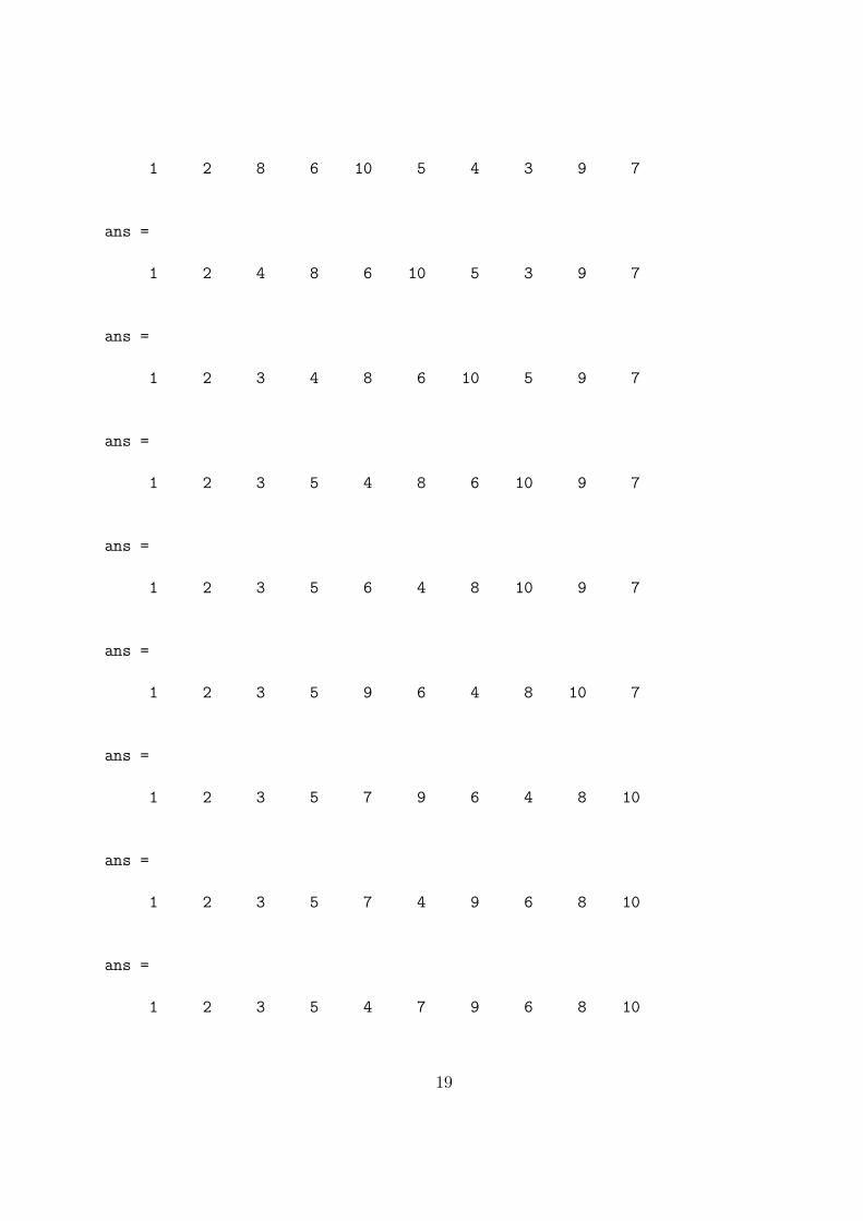
A recording of a MATLAB session follows using the data file number.dat, and as onerepresentative of the three QA heuristic m-functions, invoking insertqa.m for kblock =2. Note (a) the application of the built-in MATLAB function randperm(10) to obtain arandom input permutation of the first 10 digits; (b) the use of the utility m-function fromthe Appendix B.1, ransymat(10), to generate a target matrix targlin based on an equally(and unit) spaced set of coordinates; (c) the mechanism through the use of a “for i = 1:18”loop for displaying the permutations identified from INPERM to OUTPERM; and (d) the identifiedOUTPERM here for a QA task relying on an equally-spaced set of coordinates turns out to bethe same as found for our (globally optimal) DP solution for LUS in the L2 norm.

load number.dat

[prox10 targlin targcir] = ransymat(10);

targlin

targlin =

0 1 2 3 4 5 6 7 8 9

1 0 1 2 3 4 5 6 7 8

2 1 0 1 2 3 4 5 6 7

3 2 1 0 1 2 3 4 5 6

4 3 2 1 0 1 2 3 4 5

5 4 3 2 1 0 1 2 3 4

6 5 4 3 2 1 0 1 2 3

7 6 5 4 3 2 1 0 1 2

8 7 6 5 4 3 2 1 0 1

9 8 7 6 5 4 3 2 1 0

inperm = randperm(10)

inperm =

10 5 6 8 4 3 1 9 7 2

16

kblock = 2

kblock =

2

[outperm rawindex allperms index] = ...

insertqa(number,targlin,inperm,kblock)

elapsed_time =

0.0600

outperm =

1 2 3 5 4 6 7 9 10 8

rawindex =

206.4920

allperms =

Columns 1 through 4

[1x10 double] [1x10 double] [1x10 double] [1x10 double]

Columns 5 through 8





17



[1x10 double] [1x10 double]

index =

18

for i = 1:18

allpermsi

end

ans =

10 5 6 8 4 3 1 9 7 2

ans =

6 10 5 8 4 3 1 9 7 2

ans =

8 6 10 5 4 3 1 9 7 2

ans =

1 8 6 10 5 4 3 9 7 2

ans =

2 1 8 6 10 5 4 3 9 7

ans =

18

1 2 8 6 10 5 4 3 9 7

ans =

1 2 4 8 6 10 5 3 9 7

ans =

1 2 3 4 8 6 10 5 9 7

ans =

1 2 3 5 4 8 6 10 9 7

ans =

1 2 3 5 6 4 8 10 9 7

ans =

1 2 3 5 9 6 4 8 10 7

ans =

1 2 3 5 7 9 6 4 8 10

ans =

1 2 3 5 7 4 9 6 8 10

ans =

1 2 3 5 4 7 9 6 8 10

19

ans =

1 2 3 5 4 7 6 9 8 10

ans =

1 2 3 5 4 6 7 9 8 10

ans =

1 2 3 5 4 6 7 10 9 8

ans =

1 2 3 5 4 6 7 9 10 8

The MATLAB function uniscalqa.m

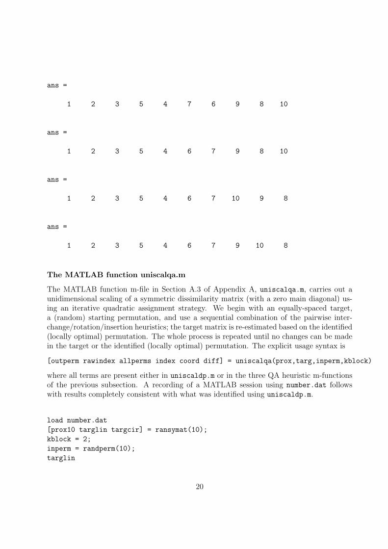
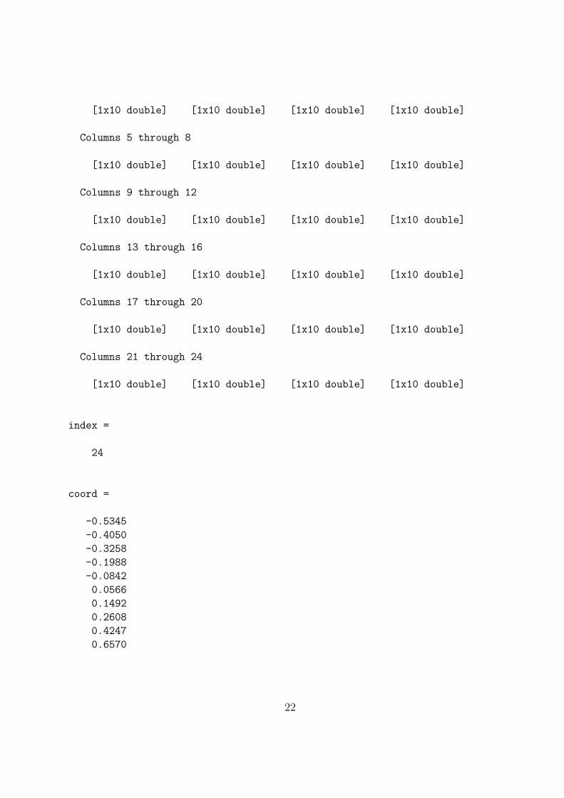
The MATLAB function m-file in Section A.3 of Appendix A, uniscalqa.m, carries out aunidimensional scaling of a symmetric dissimilarity matrix (with a zero main diagonal) us-ing an iterative quadratic assignment strategy. We begin with an equally-spaced target,a (random) starting permutation, and use a sequential combination of the pairwise inter-change/rotation/insertion heuristics; the target matrix is re-estimated based on the identified(locally optimal) permutation. The whole process is repeated until no changes can be madein the target or the identified (locally optimal) permutation. The explicit usage syntax is

[outperm rawindex allperms index coord diff] = uniscalqa(prox,targ,inperm,kblock)

where all terms are present either in uniscaldp.m or in the three QA heuristic m-functionsof the previous subsection. A recording of a MATLAB session using number.dat followswith results completely consistent with what was identified using uniscaldp.m.

load number.dat


kblock = 2;

inperm = randperm(10);

targlin

20

targlin =

0 1 2 3 4 5 6 7 8 9

1 0 1 2 3 4 5 6 7 8

2 1 0 1 2 3 4 5 6 7

3 2 1 0 1 2 3 4 5 6

4 3 2 1 0 1 2 3 4 5

5 4 3 2 1 0 1 2 3 4

6 5 4 3 2 1 0 1 2 3

7 6 5 4 3 2 1 0 1 2

8 7 6 5 4 3 2 1 0 1

9 8 7 6 5 4 3 2 1 0

inperm

inperm =

10 5 6 8 4 3 1 9 7 2

[outperm rawindex allperms index coord diff] = ...

uniscalqa(number,targlin,inperm,kblock)

elapsed_time =

0.0600

outperm =

8 10 9 7 6 4 5 3 2 1

rawindex =

26.1594

allperms =

Columns 1 through 4

21


Columns 5 through 8










index =

24

coord =

-0.5345

-0.4050

-0.3258

-0.1988

-0.0842

0.0566

0.1492

0.2608

0.4247

0.6570

22

diff =

1.9599

1.1.3 Gradient-Based Optimization

In Guttman’s 1968 paper on multidimensional scaling, the optimization task in (1) is treatedas a special case of his general iterative algorithm based on the partial derivatives of (1) withrespect to the unknown locations. For one dimension, Guttman’s multidimensional scalingalgorithm reduces to a simple updating procedure:

x(t+1)i =

1

n

n∑j=1

pijsign(x(t)i − x

(t)j ), (1.5)

where t is the index of iteration. As pointed out by de Leeuw and Heiser (1977), convergence

of (1.5) is guaranteed because x(t+1)i only depends on the rank order of x

(t)1 , . . . , x(t)

n , there area finite number of different rank orders, and no rank order can be repeated with intermediatedifferent rank orders. In fact, the stationary points of (1.5) are defined by all possibleorderings of P that lead to monotonic forms. Specifically, if x1, . . . , xn is a stationary pointof (1.5) and ρ is the permutation for which xρ(1) ≤ xρ(2) ≤ · · · ≤ xρ(n), then pρ(i)ρ(j) is

monotonic, i.e., t(ρ)1 ≤ · · · ≤ t(ρ)

n , and, in fact, t(ρ)i = xρ(i) for 1 ≤ i ≤ n. Conversely, if pij

is monotonic, then (1.5) converges in one step if we let the initial value of xi be, say, i for1 ≤ i ≤ n.

Guttman’s updating algorithm is in reality a procedure for finding monotonic forms fora proximity matrix and only very indirectly can it even be characterized as a strategy forunidimensional scaling. From a somewhat wider perspective, the general weakness of themonotonic forms for a given matrix may indicate why multidimensional scaling methodsgenerally have such difficulties with local optima when restricted to a single dimension (e.g.,see Shepard, 1974, pp. 378–379). As can be seen in the way the index of goodness-of-fit isrewritten in (1.3), the crucial quantity for distinguishing among different monotonic forms is∑

i(t(ρ)i )2. Unfortunately, consideration of this latter term disappears in Guttman’s update

method because of the algorithm’s reliance on a gradient approach.

The MATLAB function guttorder.m

The MATLAB m-function in Section A.4 of Appendix A, guttorder.m, carries out a unidi-mensional scaling of a symmetric proximity matrix based on the Guttman update formulain (1.5). The usage syntax is

[gcoordsort gperm] = guttorder(prox,inperm)

where PROX and INPERM are as before, and the output vector GCOORDSORT contains thecoordinates ordered from the most negative to most positive; GPERM is the object permutation

23

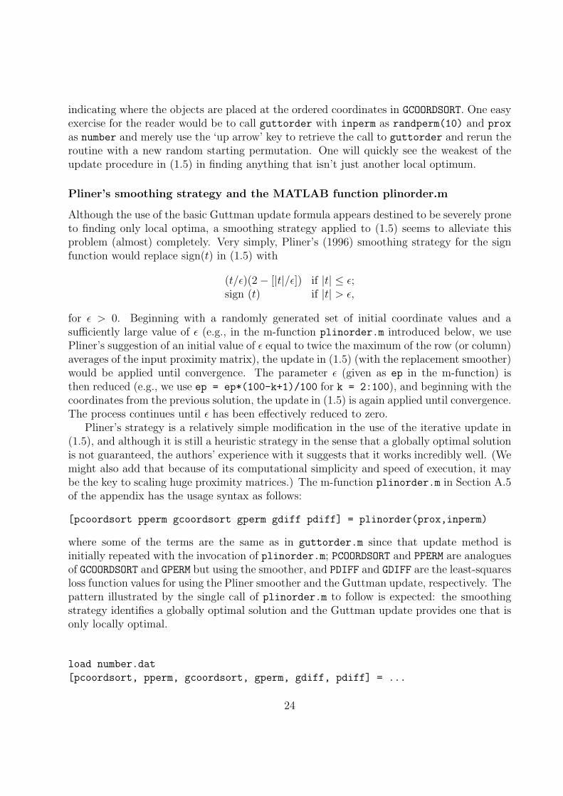
indicating where the objects are placed at the ordered coordinates in GCOORDSORT. One easyexercise for the reader would be to call guttorder with inperm as randperm(10) and prox

as number and merely use the ‘up arrow’ key to retrieve the call to guttorder and rerun theroutine with a new random starting permutation. One will quickly see the weakest of theupdate procedure in (1.5) in finding anything that isn’t just another local optimum.

Pliner’s smoothing strategy and the MATLAB function plinorder.m

Although the use of the basic Guttman update formula appears destined to be severely proneto finding only local optima, a smoothing strategy applied to (1.5) seems to alleviate thisproblem (almost) completely. Very simply, Pliner’s (1996) smoothing strategy for the signfunction would replace sign(t) in (1.5) with

(t/ε)(2− [|t|/ε]) if |t| ≤ ε;sign (t) if |t| > ε,

for ε > 0. Beginning with a randomly generated set of initial coordinate values and asufficiently large value of ε (e.g., in the m-function plinorder.m introduced below, we usePliner’s suggestion of an initial value of ε equal to twice the maximum of the row (or column)averages of the input proximity matrix), the update in (1.5) (with the replacement smoother)would be applied until convergence. The parameter ε (given as ep in the m-function) isthen reduced (e.g., we use ep = ep*(100-k+1)/100 for k = 2:100), and beginning with thecoordinates from the previous solution, the update in (1.5) is again applied until convergence.The process continues until ε has been effectively reduced to zero.

Pliner’s strategy is a relatively simple modification in the use of the iterative update in(1.5), and although it is still a heuristic strategy in the sense that a globally optimal solutionis not guaranteed, the authors’ experience with it suggests that it works incredibly well. (Wemight also add that because of its computational simplicity and speed of execution, it maybe the key to scaling huge proximity matrices.) The m-function plinorder.m in Section A.5of the appendix has the usage syntax as follows:

[pcoordsort pperm gcoordsort gperm gdiff pdiff] = plinorder(prox,inperm)

where some of the terms are the same as in guttorder.m since that update method isinitially repeated with the invocation of plinorder.m; PCOORDSORT and PPERM are analoguesof GCOORDSORT and GPERM but using the smoother, and PDIFF and GDIFF are the least-squaresloss function values for using the Pliner smoother and the Guttman update, respectively. Thepattern illustrated by the single call of plinorder.m to follow is expected: the smoothingstrategy identifies a globally optimal solution and the Guttman update provides one that isonly locally optimal.

load number.dat

[pcoordsort, pperm, gcoordsort, gperm, gdiff, pdiff] = ...

24

plinorder(number,randperm(10))

pcoordsort =

-0.5345

-0.4050

-0.3258

-0.1988

-0.0842

0.0566

0.1492

0.2608

0.4247

0.6570

pperm =

8 10 9 7 6 4 5 3 2 1

gcoordsort =

-0.5345

-0.3829

-0.2800

-0.1808

-0.0572

0.0982

0.1192

0.2708

0.2902

0.6570

gperm =

8 2 10 4 7 3 6 9 5 1

gdiff =

25

3.4425

pdiff =

1.9599

1.1.4 A Nonlinear Programming Heuristic

In considering the unidimensional scaling task in (1), Lau, Leung, and Tse (1998) note theequivalence to the minimization over x1, x2, . . . , xn of∑

i<j

min[pij − (xi − xj)]2, [pij − (xj − xi)]

2. (1.6)

Two zero/one variables can then be defined, w1ij and w2ij, and (1.6) rewritten as the math-ematical program

minimize∑i<j

w1ij(e1ij)2 + w2ij(e2ij)

2 (1.7)

subject topij = xi − xj + e1ij;

pij = xj − xi + e2ij;

w1ij + w2ij = 1;

w1ij, w2ij ≥ 0,

where e1ij is the error if xi > xj and e2ij is the error if xi < xj. The authors observe that thebinary restriction on w1ij and w2ij can be removed since they will automatically be forcedto zero or one. In short, what initially appears as a combinatorial optimization task in (1)has now been replaced by a nonlinear programming model in (1.7).

The MATLAB function unifitl2nlp.m

The m-function unifitl2nlp.m given in Section A.6 carries out the optimization task speci-fied in (1.7) by a call to a very general m-function from the MATLAB Optimization Toolbox,fmincon.m. The latter is an extremely general routine for the minimization of a constrainedmultivariable function, and requires in our case a separate m-function, objfunl2.m, thatwe give in Section A.6.1 to evaluate the objective function in (1.7). So, to use the func-tion unifitl2nlp.m, the user needs to have the Optimization Toolbox installed. The usagesyntax for unifitl2nlp.m has the form

[startcoord begval outcoord endval exitflag] = unifitl2nlp(prox,inperm)

26

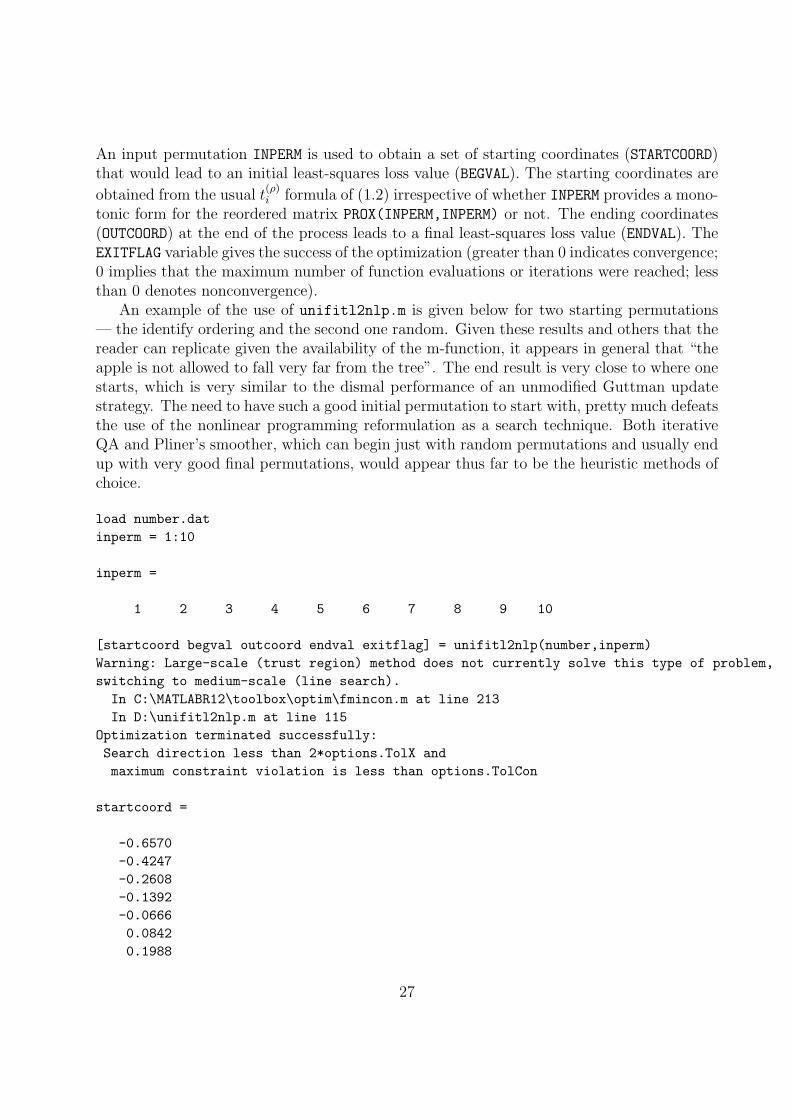
An input permutation INPERM is used to obtain a set of starting coordinates (STARTCOORD)that would lead to an initial least-squares loss value (BEGVAL). The starting coordinates are

obtained from the usual t(ρ)i formula of (1.2) irrespective of whether INPERM provides a mono-

tonic form for the reordered matrix PROX(INPERM,INPERM) or not. The ending coordinates(OUTCOORD) at the end of the process leads to a final least-squares loss value (ENDVAL). TheEXITFLAG variable gives the success of the optimization (greater than 0 indicates convergence;0 implies that the maximum number of function evaluations or iterations were reached; lessthan 0 denotes nonconvergence).

An example of the use of unifitl2nlp.m is given below for two starting permutations— the identify ordering and the second one random. Given these results and others that thereader can replicate given the availability of the m-function, it appears in general that “theapple is not allowed to fall very far from the tree”. The end result is very close to where onestarts, which is very similar to the dismal performance of an unmodified Guttman updatestrategy. The need to have such a good initial permutation to start with, pretty much defeatsthe use of the nonlinear programming reformulation as a search technique. Both iterativeQA and Pliner’s smoother, which can begin just with random permutations and usually endup with very good final permutations, would appear thus far to be the heuristic methods ofchoice.

load number.datinperm = 1:10

inperm =

1 2 3 4 5 6 7 8 9 10

[startcoord begval outcoord endval exitflag] = unifitl2nlp(number,inperm)Warning: Large-scale (trust region) method does not currently solve this type of problem,switching to medium-scale (line search).

In C:\MATLABR12\toolbox\optim\fmincon.m at line 213In D:\unifitl2nlp.m at line 115

Optimization terminated successfully:Search direction less than 2*options.TolX andmaximum constraint violation is less than options.TolCon

startcoord =

-0.6570-0.4247-0.2608-0.1392-0.06660.08420.1988

27

0.36270.40580.4968

begval =

2.1046

outcoord =

-0.6570-0.4247-0.2608-0.1392-0.06660.08420.19880.36270.40580.4968

endval =

2.1046

exitflag =

1

[startcoord begval outcoord endval exitflag] = unifitl2nlp(number,randperm(10))Warning: Large-scale (trust region) method does not currently solve this type of problem,switching to medium-scale (line search).In C:\MATLABR12\toolbox\optim\fmincon.m at line 213In D:\unifitl2nlp.m at line 115

Warning: Divide by zero.In C:\MATLABR12\toolbox\optim\private\nlconst.m at line 198In C:\MATLABR12\toolbox\optim\fmincon.m at line 458In D:\unifitl2nlp.m at line 115

Optimization terminated successfully:Magnitude of directional derivative in search directionless than 2*options.TolFun and maximum constraint violation

28

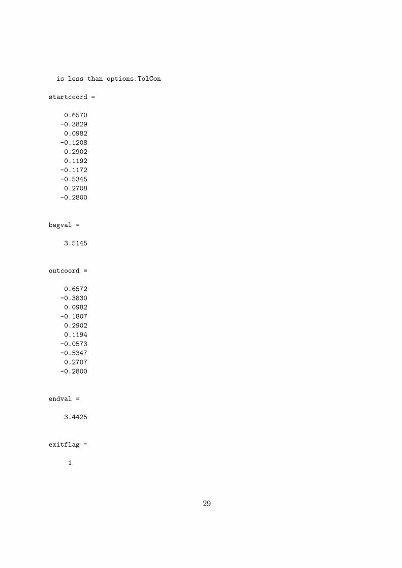
is less than options.TolCon

startcoord =

0.6570-0.38290.0982-0.12080.29020.1192-0.1172-0.53450.2708-0.2800

begval =

3.5145

outcoord =

0.6572-0.38300.0982-0.18070.29020.1194-0.0573-0.53470.2707-0.2800

endval =

3.4425

exitflag =

1

29

1.1.5 Solving Linear (In)equality Constrained Least Squares Tasks:The Example of the Confirmatory Fitting of a Given Order

A strategy for solving linear systems of equations through the use of iterative projectionand typically attributed to Kaczmarz (1937) (e.g., see Bodewig, 1956, pp. 163–164, or morerecently, Deutsch, 1992, pp. 107–108) has some very close connections with several morerecent approaches in the Applied Statistics/Psychometrics (AS/P) literature to the least-squares representation of a data matrix. The latter rely on a close relative to the Kaczmarzstrategy and what is now commonly referred to as Dykstra’s method for solving linearinequality constrained weighted least-squares tasks (e.g., see Dykstra, 1983).

Kaczmarz’s method can be characterized as follows:Given A = aij of order m× n, x′ = x1, . . . , xn, b′ = b1, . . . , bm, and assuming the

linear system Ax = b is consistent, define the set Ci = x | aijxj = bi, for 1 ≤ i ≤ m.The projection of any n × 1 vector y onto Ci is simply y − (a′iy − bi)ai(a

′iai)

−1, wherea′i = ai1, . . . , ain. Beginning with a vector x0, and successively projecting x0 onto C1, andthat result onto C2, and so on, and cyclically and repeatedly reconsidering projections ontothe sets C1, . . . , Cm, leads at convergence to a vector x∗

0 that is closest to x0 (in vector 2-norm, so

∑ni=1(x0i−x∗0i)

2 is minimized) and Ax∗0 = b. In short, Kaczmarz’s method provides

an iterative way to solve least-squares tasks subject to equality restrictions.Dykstra’s method can be characterized as follows:Given A = aij of order m × n, x′

0 = x01, . . . , x0n, b′ = b1, . . . , bm, and w′ =w1, . . . , wn, where wj > 0 for all j, find x∗

0 such that a′ix∗0 ≤ bi for 1 ≤ i ≤ m and∑n

i=1 wi(x0i−x∗0i)2 is minimized. Again, (re)define the (closed convex) sets Ci = x | aijxj ≤

bi and when a vector y /∈ Ci, its projection onto Ci (in the metric defined by the weightvector w) is y− (a′iy− bi)aiW

−1(a′iW−1ai)

−1, where W−1 = diagw−11 , . . . , w−1

n . We againinitialize the process with the vector x0 and each set C1, . . . , Cm is considered in turn. Ifthe vector being carried forward to this point when Ci is (re)considered does not satisfy theconstraint defining Ci, a projection onto Ci occurs. The sets C1, . . . , Cm are cyclically andrepeatedly considered but with one difference from the operation of Kaczmarz’s method —each time a constraint set Ci is revisited, any changes from the previous time Ci was reachedare first “added back”. This last process ensures convergence to an optimal solution x∗

0 (seeDykstra, 1983). Thus, Dykstra’s method generalizes the equality restrictions that can behandled by Kaczmarz’s strategy to the use of inequality constraints.

The Dykstra method is currently serving as the major computational tool for a varietyof newer data representation devices in AS/P. For example, and first considering an arbi-trary rectangular data matrix, Dykstra and Robertson (1982) use it to fit a least-squaresapproximation constrained by entries within rows and within columns being monotonic withrespect to given row and column orders. For an arbitrary symmetric proximity matrix A(of order p × p and with diagonal entries typically set to zero), a number of applicationsof Dykstra’s method have been discussed for approximating A in a least-squares sense by

30

A1 + · · ·+ AK , where K is typically small (e.g., 2 or 3) and each Ak is patterned in a par-ticularly informative way that can be characterized by a set of linear inequality constraintsthat its entries should satisfy. We note three exemplar classes of patterns that Ak mighthave, and all with a substantial history in the AS/P literature. In each instance, Dykstra’smethod can be used to fit the additive structures satisfying the inequality constraints oncethey are identified, possibly through an initial combinatorial optimization task seeking anoptimal reordering of a given (residual) data matrix, or in some instances in a heuristic formto identify the constraints to impose in the first place. We merely give the patterns soughtin Ak and refer the reader to sources that develop the representations in more detail.

(a) Order constraints (Hubert and Arabie, 1994): The entries in Ak = aij(k) shouldsatisfy the anti-Robinson constraints: there exists a permutation on the first p integers ρ(·)such that aρ(i)ρ(j)(k) ≤ aρ(i)ρ(j′)(k) for 1 ≤ i < j < j′ ≤ p, and aρ(i)ρ(j)(k) ≤ aρ(i′)ρ(j)(k) for1 ≤ i < i′ < j ≤ p.

(b) Ultrametric and additive trees (Hubert and Arabie, 1995): The entries in Ak shouldbe represented by an ultrametric: for all i, j, and h, aij(k) ≤ maxaih(k), ajh(k); or an additivetree: for all i, j, h, and l, aij(k) + ahl(k) ≤ maxaih(k) + ajl(k), ail(k) + ajh(k).

(c) Linear and circular unidimensional scales (Hubert, Arabie, and Meulman, 1997): Theentries in Ak should be represented by a linear unidimensional scale: aij(k) = |xj−xi| for someset of coordinates x1, . . . , xn; or a circular unidimensional scale: aij(k) = min|xj − xi|, x0 −|xj −xi| for some set of coordinates x1, . . . , xn and x0 representing the circumference of thecircular structure.

The confirmatory fitting of a given order using the MATLAB function linfit.m

The MATLAB m-function in Section A.7, linfit.m, fits a set of coordinates to a givenproximity matrix based on some given input permutation, say, ρ(0). Specifically, we seekx1 ≤ x2 ≤ · · · ≤ xn such that

∑i<j(pρ0(i)ρ0(j) − |xj − xi|)2 is minimized (and where the

permutation ρ(0) may not even put the matrix pρ0(i)ρ0(j) into a monotonic form). Usingthe syntax

[fit diff coord] = linfit(prox,inperm)

the matrix |xj − xi| is referred to as the fitted matrix (FIT); COORD gives the orderedcoordinates; and DIFF is the value of the least-squares criterion. The fitted matrix is foundthrough the Dykstra-Kaczmarz method where the equality constraints defined by distancesalong a continuum are imposed to find the fitted matrix, i.e., if i < j < k, then |xi − xj| +|xj − xk| = |xi − xk|. Once found, the actual ordered coordinates are retrieved by the usual

t(ρ0)i formula in (1.2) but computed on FIT.

The example below of the use of linfit.m fits two separate orders: the identity permu-tation and the one that we know is least-squares optimal. The consistency of the results canbe compared to those given earlier.

load number.dat

31

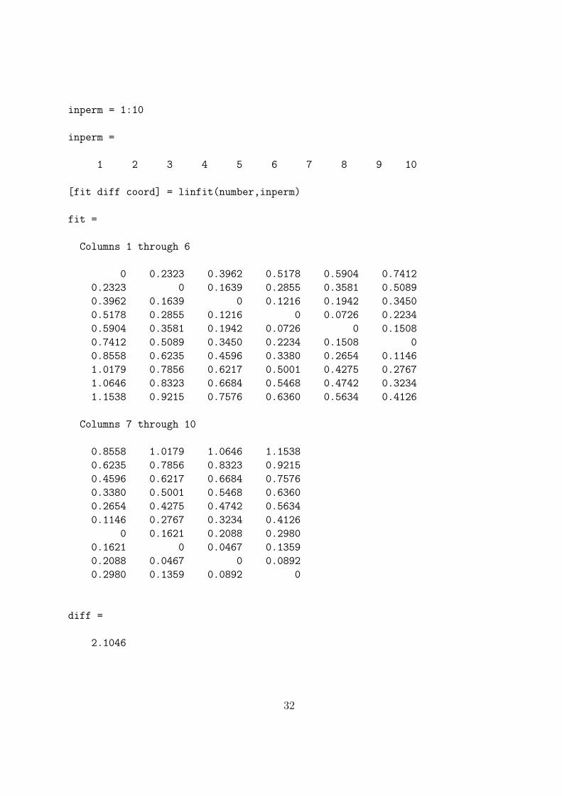
inperm = 1:10

inperm =

1 2 3 4 5 6 7 8 9 10

[fit diff coord] = linfit(number,inperm)

fit =

Columns 1 through 6

0 0.2323 0.3962 0.5178 0.5904 0.7412

0.2323 0 0.1639 0.2855 0.3581 0.5089

0.3962 0.1639 0 0.1216 0.1942 0.3450

0.5178 0.2855 0.1216 0 0.0726 0.2234

0.5904 0.3581 0.1942 0.0726 0 0.1508

0.7412 0.5089 0.3450 0.2234 0.1508 0

0.8558 0.6235 0.4596 0.3380 0.2654 0.1146

1.0179 0.7856 0.6217 0.5001 0.4275 0.2767

1.0646 0.8323 0.6684 0.5468 0.4742 0.3234

1.1538 0.9215 0.7576 0.6360 0.5634 0.4126


0.8558 1.0179 1.0646 1.1538

0.6235 0.7856 0.8323 0.9215

0.4596 0.6217 0.6684 0.7576

0.3380 0.5001 0.5468 0.6360

0.2654 0.4275 0.4742 0.5634

0.1146 0.2767 0.3234 0.4126

0 0.1621 0.2088 0.2980

0.1621 0 0.0467 0.1359

0.2088 0.0467 0 0.0892

0.2980 0.1359 0.0892 0

diff =

2.1046

32

coord =

-0.6570

-0.4247

-0.2608

-0.1392

-0.0666

0.0842

0.1988

0.3627

0.4058

0.4968

inperm = [8 10 9 7 6 4 5 3 2 1]

inperm =

8 10 9 7 6 4 5 3 2 1


fit =

Columns 1 through 6

0 0.1295 0.2087 0.3357 0.4503 0.5911

0.1295 0 0.0792 0.2062 0.3208 0.4616

0.2087 0.0792 0 0.1270 0.2416 0.3824

0.3357 0.2062 0.1270 0 0.1146 0.2554

0.4503 0.3208 0.2416 0.1146 0 0.1408

0.5911 0.4616 0.3824 0.2554 0.1408 0

0.6837 0.5542 0.4750 0.3480 0.2334 0.0926

0.7953 0.6658 0.5866 0.4596 0.3450 0.2042

0.9592 0.8297 0.7505 0.6235 0.5089 0.3681

1.1915 1.0620 0.9828 0.8558 0.7412 0.6004


0.6837 0.7953 0.9592 1.1915

0.5542 0.6658 0.8297 1.0620

0.4750 0.5866 0.7505 0.9828

0.3480 0.4596 0.6235 0.8558

33

0.2334 0.3450 0.5089 0.7412

0.0926 0.2042 0.3681 0.6004

0 0.1116 0.2755 0.5078

0.1116 0 0.1639 0.3962

0.2755 0.1639 0 0.2323

0.5078 0.3962 0.2323 0

diff =

1.9599

coord =

-0.5345

-0.4050

-0.3258

-0.1988

-0.0842

0.0566

0.1492

0.2608

0.4247

0.6570

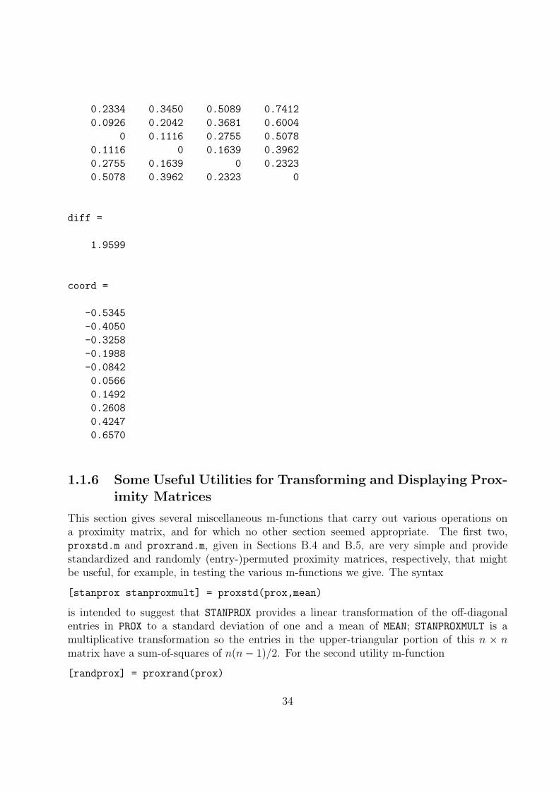
1.1.6 Some Useful Utilities for Transforming and Displaying Prox-imity Matrices

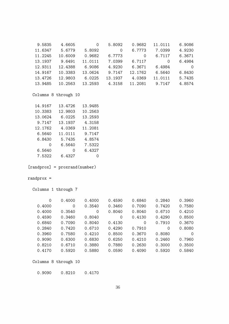
This section gives several miscellaneous m-functions that carry out various operations ona proximity matrix, and for which no other section seemed appropriate. The first two,proxstd.m and proxrand.m, given in Sections B.4 and B.5, are very simple and providestandardized and randomly (entry-)permuted proximity matrices, respectively, that mightbe useful, for example, in testing the various m-functions we give. The syntax

[stanprox stanproxmult] = proxstd(prox,mean)

is intended to suggest that STANPROX provides a linear transformation of the off-diagonalentries in PROX to a standard deviation of one and a mean of MEAN; STANPROXMULT is amultiplicative transformation so the entries in the upper-triangular portion of this n × nmatrix have a sum-of-squares of n(n− 1)/2. For the second utility m-function

[randprox] = proxrand(prox)

34

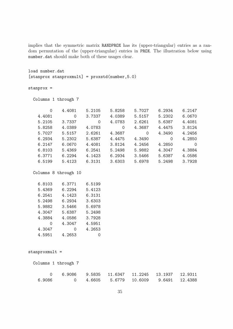
implies that the symmetric matrix RANDPROX has its (upper-triangular) entries as a ran-dom permutation of the (upper-triangular) entries in PROX. The illustration below usingnumber.dat should make both of these usages clear.

load number.dat

[stanprox stanproxmult] = proxstd(number,5.0)

stanprox =

Columns 1 through 7

0 4.4081 5.2105 5.8258 5.7027 6.2934 6.2147

4.4081 0 3.7337 4.0389 5.5157 5.2302 6.0670

5.2105 3.7337 0 4.0783 2.6261 5.6387 4.4081

5.8258 4.0389 4.0783 0 4.3687 4.4475 3.8124

5.7027 5.5157 2.6261 4.3687 0 4.3490 4.2456

6.2934 5.2302 5.6387 4.4475 4.3490 0 4.2850

6.2147 6.0670 4.4081 3.8124 4.2456 4.2850 0

6.8103 5.4369 6.2541 5.2498 5.9882 4.3047 4.3884

6.3771 6.2294 4.1423 6.2934 3.5466 5.6387 4.0586

6.5199 5.4123 6.3131 3.6303 5.6978 5.2498 3.7928


6.8103 6.3771 6.5199

5.4369 6.2294 5.4123

6.2541 4.1423 6.3131

5.2498 6.2934 3.6303

5.9882 3.5466 5.6978

4.3047 5.6387 5.2498

4.3884 4.0586 3.7928

0 4.3047 4.5951

4.3047 0 4.2653

4.5951 4.2653 0

stanproxmult =

Columns 1 through 7

0 6.9086 9.5835 11.6347 11.2245 13.1937 12.9311

6.9086 0 4.6605 5.6779 10.6009 9.6491 12.4388

35

9.5835 4.6605 0 5.8092 0.9682 11.0111 6.9086

11.6347 5.6779 5.8092 0 6.7773 7.0399 4.9230

11.2245 10.6009 0.9682 6.7773 0 6.7117 6.3671

13.1937 9.6491 11.0111 7.0399 6.7117 0 6.4984

12.9311 12.4388 6.9086 4.9230 6.3671 6.4984 0

14.9167 10.3383 13.0624 9.7147 12.1762 6.5640 6.8430

13.4726 12.9803 6.0225 13.1937 4.0369 11.0111 5.7435

13.9485 10.2563 13.2593 4.3158 11.2081 9.7147 4.8574


14.9167 13.4726 13.9485

10.3383 12.9803 10.2563

13.0624 6.0225 13.2593

9.7147 13.1937 4.3158

12.1762 4.0369 11.2081

6.5640 11.0111 9.7147

6.8430 5.7435 4.8574

0 6.5640 7.5322

6.5640 0 6.4327

7.5322 6.4327 0

[randprox] = proxrand(number)

randprox =

Columns 1 through 7

0 0.4000 0.4000 0.4590 0.6840 0.2840 0.3960

0.4000 0 0.3540 0.3460 0.7090 0.7420 0.7580

0.4000 0.3540 0 0.8040 0.8040 0.6710 0.4210

0.4590 0.3460 0.8040 0 0.4130 0.4290 0.8500

0.6840 0.7090 0.8040 0.4130 0 0.7910 0.3670

0.2840 0.7420 0.6710 0.4290 0.7910 0 0.8080

0.3960 0.7580 0.4210 0.8500 0.3670 0.8080 0

0.9090 0.6300 0.6830 0.6250 0.4210 0.2460 0.7960

0.8210 0.6710 0.3880 0.7880 0.2630 0.3000 0.3500

0.4170 0.5920 0.5880 0.0590 0.4090 0.5920 0.5840


0.9090 0.8210 0.4170

36

0.6300 0.6710 0.5920

0.6830 0.3880 0.5880

0.6250 0.7880 0.0590

0.4210 0.2630 0.4090

0.2460 0.3000 0.5920

0.7960 0.3500 0.5840

0 0.2960 0.6460

0.2960 0 0.3920

0.6460 0.3920 0

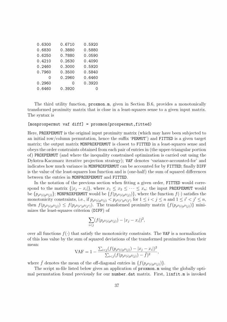
The third utility function, proxmon.m, given in Section B.6, provides a monotonicallytransformed proximity matrix that is close in a least-squares sense to a given input matrix.The syntax is

[monproxpermut vaf diff] = proxmon(proxpermut,fitted)

Here, PROXPERMUT is the original input proximity matrix (which may have been subjected toan initial row/column permutation, hence the suffix ‘PERMUT’) and FITTED is a given targetmatrix; the output matrix MONPROXPERMUT is closest to FITTED in a least-squares sense andobeys the order constraints obtained from each pair of entries in (the upper-triangular portionof) PROXPERMUT (and where the inequality constrained optimization is carried out using theDykstra-Kaczmarz iterative projection strategy); VAF denotes ‘variance-accounted-for’ andindicates how much variance in MONPROXPERMUT can be accounted for by FITTED; finally DIFF

is the value of the least-squares loss function and is (one-half) the sum of squared differencesbetween the entries in MONPROXPERMUT and FITTED.

In the notation of the previous section when fitting a given order, FITTED would corre-spond to the matrix |xj − xi|, where x1 ≤ x2 ≤ · · · ≤ xn; the input PROXPERMUT wouldbe pρ0(i)ρ0(j); MONPROXPERMUT would be f(pρ0(i)ρ0(j)), where the function f(·) satisfies themonotonicity constraints, i.e., if pρ0(i)ρ0(j) < pρ0(i′)ρ0(j′) for 1 ≤ i < j ≤ n and 1 ≤ i′ < j′ ≤ n,then f(pρ0(i)ρ0(j)) ≤ f(pρ0(i′)ρ0(j′)). The transformed proximity matrix f(pρ0(i)ρ0(j)) mini-mizes the least-squares criterion (DIFF) of∑

i<j

(f(pρ0(i)ρ0(j))− |xj − xi|)2,

over all functions f(·) that satisfy the monotonicity constraints. The VAF is a normalizationof this loss value by the sum of squared deviations of the transformed proximities from theirmean:

VAF = 1−∑

i<j(f(pρ0(i)ρ0(j))− |xj − xi|)2∑i<j(f(pρ0(i)ρ0(j))− f)2

,

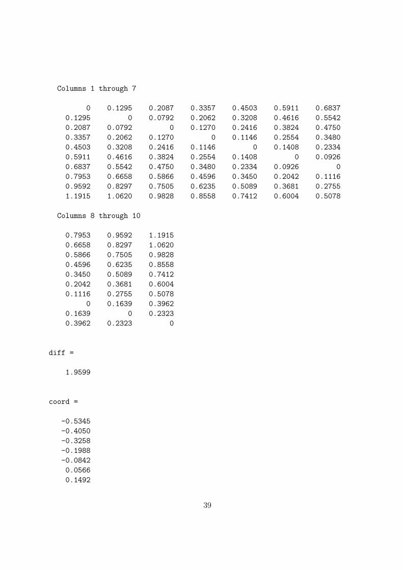
where f denotes the mean of the off-diagonal entries in f(pρ0(i)ρ0(j)).The script m-file listed below gives an application of proxmon.m using the globally opti-

mal permutation found previously for our number.dat matrix. First, linfit.m is invoked

37

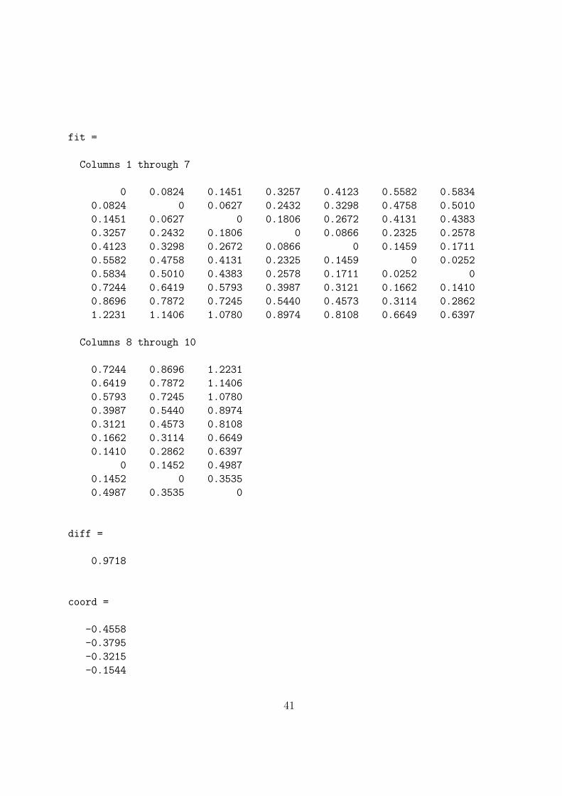
to obtain a fitted matrix (fit); proxmon.m then generates the monotonically transformedproximity matrix (monproxpermut) with vaf = .5821 and diff = 1.0623. The strategy isthen repeated cyclically (i.e., finding a fitted matrix based on the monotonically transformedproximity matrix, finding a new monotonically tranformed matrix, and so on). To avoid de-generacy (where all matrices would converge to zeros), the sum of squares of the fitted matrixis kept the same as it was initially; convergence is based on observing a minimal change (lessthan 1.0e-006) in the vaf. As indicated in the output below, the final vaf is .6672 with adiff of .9718.

load number.dat

inperm = [8 10 9 7 6 4 5 3 2 1]


[monproxpermut vaf diff] = ...

proxmon(number(inperm,inperm),fit)

sumfitsq = sum(sum(fit.^2));

prevvaf = 2;

while (abs(prevvaf-vaf) >= 1.0e-006)

prevvaf = vaf;

[fit diff coord] = linfit(monproxpermut,1:10);

sumnewfitsq = sum(sum(fit.^2));

fit = sqrt(sumfitsq)*(fit/sqrt(sumnewfitsq));

[monproxpermut vaf diff] = proxmon(number(inperm,inperm), fit);

end

fit

diff

coord

monproxpermut

vaf

inperm =

8 10 9 7 6 4 5 3 2 1

fit =

38

Columns 1 through 7

0 0.1295 0.2087 0.3357 0.4503 0.5911 0.6837

0.1295 0 0.0792 0.2062 0.3208 0.4616 0.5542

0.2087 0.0792 0 0.1270 0.2416 0.3824 0.4750

0.3357 0.2062 0.1270 0 0.1146 0.2554 0.3480

0.4503 0.3208 0.2416 0.1146 0 0.1408 0.2334

0.5911 0.4616 0.3824 0.2554 0.1408 0 0.0926

0.6837 0.5542 0.4750 0.3480 0.2334 0.0926 0

0.7953 0.6658 0.5866 0.4596 0.3450 0.2042 0.1116

0.9592 0.8297 0.7505 0.6235 0.5089 0.3681 0.2755

1.1915 1.0620 0.9828 0.8558 0.7412 0.6004 0.5078


0.7953 0.9592 1.1915

0.6658 0.8297 1.0620

0.5866 0.7505 0.9828

0.4596 0.6235 0.8558

0.3450 0.5089 0.7412

0.2042 0.3681 0.6004

0.1116 0.2755 0.5078

0 0.1639 0.3962

0.1639 0 0.2323

0.3962 0.2323 0

diff =

1.9599

coord =

-0.5345

-0.4050

-0.3258

-0.1988

-0.0842

0.0566

0.1492

39

0.2608

0.4247

0.6570

monproxpermut =

Columns 1 through 7

0 0.2701 0.2701 0.2701 0.2701 0.5380 0.6536

0.2701 0 0.2701 0.2701 0.4148 0.2701 0.5380

0.2701 0.2701 0 0.2701 0.5380 0.6960 0.2701

0.2701 0.2701 0.2701 0 0.2701 0.2701 0.2701

0.2701 0.4148 0.5380 0.2701 0 0.2701 0.2701

0.5380 0.2701 0.6960 0.2701 0.2701 0 0.2701

0.6536 0.5380 0.2701 0.2701 0.2701 0.2701 0

0.6960 0.7035 0.2701 0.2701 0.5380 0.2701 0.1116

0.5380 0.5380 0.6960 0.6536 0.4148 0.2701 0.5380

1.1915 1.0620 0.9828 0.6960 0.7035 0.6004 0.5380


0.6960 0.5380 1.1915

0.7035 0.5380 1.0620

0.2701 0.6960 0.9828

0.2701 0.6536 0.6960

0.5380 0.4148 0.7035

0.2701 0.2701 0.6004

0.1116 0.5380 0.5380

0 0.2701 0.3962

0.2701 0 0.2701

0.3962 0.2701 0

vaf =

0.5821

diff =

1.0623

40

fit =

Columns 1 through 7

0 0.0824 0.1451 0.3257 0.4123 0.5582 0.5834

0.0824 0 0.0627 0.2432 0.3298 0.4758 0.5010

0.1451 0.0627 0 0.1806 0.2672 0.4131 0.4383

0.3257 0.2432 0.1806 0 0.0866 0.2325 0.2578

0.4123 0.3298 0.2672 0.0866 0 0.1459 0.1711

0.5582 0.4758 0.4131 0.2325 0.1459 0 0.0252

0.5834 0.5010 0.4383 0.2578 0.1711 0.0252 0

0.7244 0.6419 0.5793 0.3987 0.3121 0.1662 0.1410

0.8696 0.7872 0.7245 0.5440 0.4573 0.3114 0.2862

1.2231 1.1406 1.0780 0.8974 0.8108 0.6649 0.6397


0.7244 0.8696 1.2231

0.6419 0.7872 1.1406

0.5793 0.7245 1.0780

0.3987 0.5440 0.8974

0.3121 0.4573 0.8108

0.1662 0.3114 0.6649

0.1410 0.2862 0.6397

0 0.1452 0.4987

0.1452 0 0.3535

0.4987 0.3535 0

diff =

0.9718

coord =

-0.4558

-0.3795

-0.3215

-0.1544

41

-0.0742

0.0609

0.0842

0.2147

0.3492

0.6764

monproxpermut =

Columns 1 through 7

0 0.2612 0.2458 0.2612 0.2458 0.5116 0.6080

0.2612 0 0.2458 0.2458 0.4286 0.2458 0.5116

0.2458 0.2458 0 0.2458 0.5116 0.6899 0.2458

0.2612 0.2458 0.2458 0 0.2458 0.2458 0.2458

0.2458 0.4286 0.5116 0.2458 0 0.2612 0.2458

0.5116 0.2458 0.6899 0.2458 0.2612 0 0.2458

0.6080 0.5116 0.2458 0.2458 0.2458 0.2458 0

0.6899 0.7264 0.2458 0.2612 0.5116 0.2458 0.1410

0.5116 0.5116 0.6899 0.6080 0.4286 0.2458 0.5116

1.2231 1.1406 1.0780 0.6899 0.7264 0.6080 0.6080


0.6899 0.5116 1.2231

0.7264 0.5116 1.1406

0.2458 0.6899 1.0780

0.2612 0.6080 0.6899

0.5116 0.4286 0.7264

0.2458 0.2458 0.6080

0.1410 0.5116 0.6080

0 0.2458 0.4286

0.2458 0 0.2612

0.4286 0.2612 0

vaf =

0.6672

42

The final m-function of this miscellany section, matcolor.m, and given in Section B.7,provides a way of displaying a set of permutations constructed for a proximity matrix (asmight be obtained, say, from one of the QA interchange routines) in a color-coded manner.The usage syntax is

matcolor(datamat,perms,numperms)

where DATAMAT is an n × n symmetric proximity matrix; PERMS is a cell array containingNUMPERMS permutations. A movie is constructed and played that illustrates the transforma-tions carried out on the proximity matrix from the first permutation, perms1, to the last,permsnumperms. The colormap used in this example is ‘summer’, but a variety of otheralternatives are available within the MATLAB environment.

To give an example of the use of matcolor.m, the MATLAB statements given belowshould be entered by the reader; stand back and enjoy the movie.

load number.dat


inperm = randperm(10);

[outperm,rawindex,allperms,index] = ...

pairwiseqa(number,targlin,inperm);

matcolor(number,allperms,index)

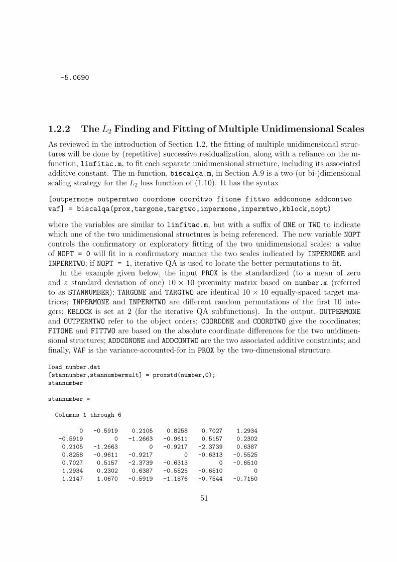
1.2 The Incorporation of Additive Constants in L2 LUS

Thus far in Chapter 1 the emphasis has been solely on the basic unidimensional scaling modelin (1), where we seek a set of n coordinates x1, . . . , xn so the interpoint distances |xj − xi|are close in a least-squares sense to the proximities pij (1 ≤ i, j ≤ n). This section willextend this simple linear unidimensional scaling (LUS) structure to one that incorporates anadditional additive constant. Explicitly, we consider the slightly more general least-squaresloss function of the form ∑

i<j

(pij + c− |xj − xi|)2, (1.8)

or equivalently, ∑i<j

(pij − |xj − xi| − c)2, (1.9)

where c is some constant to be estimated along with the coordinates x1, . . . , xn. The opti-mization task implicit in the use of (1.8) and (1.9) can be interpreted in either of two ways,as reflected by the equality of the two forms of the loss function: (a) the interpoint distancesamong a set of n coordinates along a line, |xj − xi|, are being fitted to a constant trans-lation of the originally given proximities, pij + c; or (b) a generalization from the usualunidimensional model to one of the form |xj−xi|−c is being fitted to the proximities pijoriginally given. Although these two interpretations will not affect how we presently proceed,

43

the second, which includes the additive constant as a part of the model, will become relevantin how generalizations are framed in Section 1.2.2 concerning the fitting of multiple unidi-mensional structures to a given proximity matrix. In any case, the presence of the constantc in (1.8) and (1.9) obviates the need to impose any type of non-negativity constraints onthe input proximities (in fact, for consistency of presentation, we routinely begin with prox-imities standardized to a mean of zero and standard deviation of one as a way of providingsome type of common interpretive scale for whatever proximities we may be originally given,although such a transformation is not necessary for the methods of optimization pursued).This step of estimating an additive constant may seem like a minor modification at first, butthe presence of negative proximities can produce rather serious difficulties in discussions oflinear unidimensional scaling; e.g., they cannot be accommodated in Pliner’s (1996) sugges-tion of a smooth gradient approximation, and their presence invalidates several convenientproperties or characterizations that certain optimization heuristics would otherwise possess.In various related optimization tasks, specialized algorithms have been devised to deal withthe possibility of negative proximities, however they might arise (see Heiser, 1989, 1991).

The discussion in the previous sections has been restricted to the fitting of a singleunidimensional structure to a symmetric proximity matrix. Given the type of computationalapproach being developed here for carrying out this task that lack dependence on the presenceof non-negative proximities, extensions are very direct to the use of multiple unidimensionalstructures through a process of successive residualization of the original proximity matrix.For example, the fitting of two LUS structures to a proximity matrix pij could be rephrasedas the minimization of a least squares loss function that generalizes (1.9) to the form∑

i<j

(pij − [|xj1 − xi1| − c1]− [|xj2 − xi2| − c2])2. (1.10)

The attempt to minimize (1.10) could proceed with the fitting of a single LUS structure topij, [|xj1−xi1| − c1], using the iterative QA procedure of section 1.1.2, and once obtained,fitting a second LUS structure, [|xj2 − xi2| − c2], to the residual matrix, pij − [|xj1 − xi1| −c1]. The process would then cycle by repetitively fitting the residuals from the secondlinear structure by the first, and the residuals from the first linear structure by the second,until the sequence converges. In any case, obvious extensions would exist for (1.10) to theinclusion of more than two LUS structures, or even to the eventual mixture of other typesof representations in the spirit of Carroll and Pruzansky’s (1980) hybrid models.

The explicit inclusion of two constants, c1 and c2 in (1.10) rather than adding these twotogether and including a single additive constant c, deserves some additional explanation.In the case of fitting a single LUS structure using the loss functions in (1.8) and (1.9), it wasnoted in the introduction that two interpretations exist for the role of the additive constantc. We could consider |xj − xi| to be fitted to the translated proximities pij + c, oralternatively, |xj −xi|− c to be fitted to the original proximities pij, where the constantc becomes part of the actual model. Although these two interpretations do not lead to anyalgorithmic differences in how we would proceed with minimizing the loss functions in (1.8)and (1.9), a consistent use of the second interpretation suggests that we frame extensions to

44

the use of multiple LUS structures as we did in (1.10), where it is explicit that the constantsc1 and c2 are part of the actual models to be fitted to the (untransformed) proximities pij.Once c1 and c2 are obtained, they could be summed as c = c1 + c2, and an interpretationmade that we have attempted to fit a transformed set of proximities pij + c by the sum|xj1 − xi1|+ |xj2 − xi2| (and in this latter case, a more usual terminology would be one ofa two-dimensional scaling (MDS) based on the city-block distance function). However, sucha further interpretation is unnecessary and could lead to at least some small terminologicalconfusion in further extensions that we might wish to pursue. For instance, if some typeof (optimal nonlinear) transformation, say f(·), of the proximities is also sought (e.g., amonotonic function of some form as in Section 1.2.3 below) in addition to fitting multipleLUS structures, and where pij in (1.10) is replaced by f(pij), and f(·) is to be constructed,the first interpretation would require the use of a ‘doubly transformed’ set of proximitiesf(pij) + c to be fitted by the sum |xj1 − xi1| + |xj2 − xi2|. In general, it seems bestto avoid the need to incorporate the notion of a double transformation in this context, andinstead merely consider the constants c1 and c2 to be part of the models being fitted to atransformed set of proximities f(pij).

1.2.1 The L2 Fitting of a Single Unidimensional Scale (with anAdditive Constant)

Given a fixed object permutation, ρ(0), we denote the set of all n × n matrices that areadditive translations of the off-diagonal entries in the reordered symmetric proximity matrixpρ(0)(i)ρ(0)(j) by ∆ρ(0) , and let Ξ be the set of all n×n matrices that represent the interpointdistances between all pairs of n coordinate locations along a line. Explicitly,

∆ρ(0) ≡ qij|qij = pρ(0)(i)ρ(0)(j) + c, for some constant c, i 6= j; qii = 0, 1 ≤ i ≤ n;

Ξ ≡ rij|rij = |xj − xi| for some set of n coordinates, x1 ≤ · · · ≤ xn;∑

i

xi = 0.

Alternatively, we could define Ξ through a set of linear inequality (for non-negativity re-strictions) and equality constraints (to represent the additive nature of distances along aline – as we did in linfit.m). In any case, both ∆ρ(0) and Ξ are closed convex sets (in aHilbert space), and thus, given any n × n symmetric matrix with a zero main diagonal, itsprojection onto either ∆ρ(0) or Ξ exists, i.e., there is a (unique) member of ∆ρ(0) or Ξ ata closest (Euclidean) distance to the given matrix (e.g., see Cheney and Goldstein, 1959).Moreover, if a procedure of alternating projections onto ∆ρ(0) and Ξ is carried out (where agiven matrix is first projected onto one of the sets, and that result is then projected ontothe second which result is in turn projected back onto the first, and so on), the process isconvergent and generates members of ∆ρ(0) and Ξ that are closest to each other (again, thislast statement is justified in Cheney and Goldstein, 1959, Theorems 2 and 4).

Given any n × n symmetric matrix with a main diagonal of all zeros, which we denotearbitrarily as U = uij, its projection onto ∆ρ(0) may be obtained by a simple formula for

45

the sought constant c. Explicitly, the minimum over c of∑i<j

(pρ(0)(i)ρ(0)(j)+ c− uij)2,

is obtained forc = (2/n(n− 1))

∑i<j

(uij − pρ(0)(i)ρ(0)(j)),

and thus, this last value defines a constant translation of the proximities necessary to generatethat member of ∆ρ(0) closest to U = uij. For the second necessary projection and given anyn× n symmetric matrix (again with a main diagonal of all zeros, that we denote arbitrarilyas V = vij (but which in our applications will generally have the form vij = pρ(0)(i)ρ(0)(j) +cfor i 6= j and some constant c), its projection onto Ξ is somewhat more involved and requiresminimizing ∑

i<j

(vij − rij)2,

over rij, where rij is subject to the linear inequality nonnegativity constraints, and thelinear equality constraints of representing distances along a line (of the set Ξ). Althoughthis is a (classic) quadratic programming problem for which a wide variety of optimizationtechniques has been published, we adopt (as we did in fitting a LUS without an additiveconstant in linfit.m, the Dykstra-Kaczmarz iterative projection strategy that we reviewedearlier in Section 1.1.5).

The MATLAB function linfitac.m

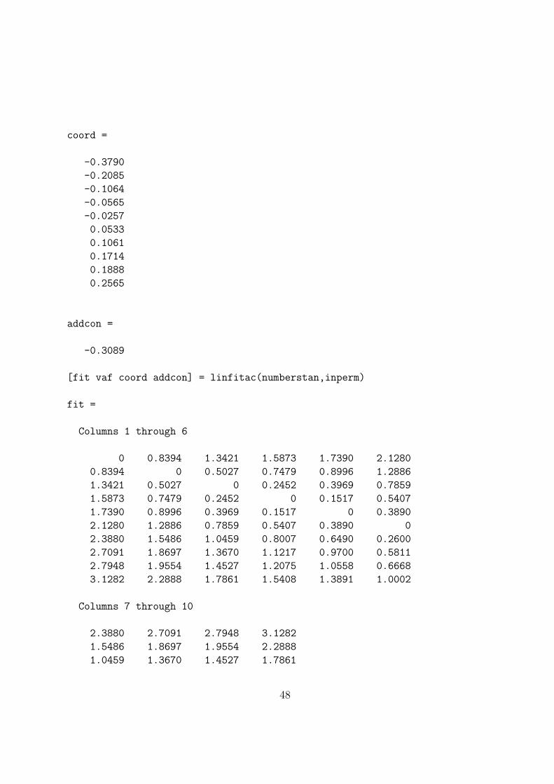
As discussed above, the MATLAB m-function in Section A.8, linfitac.m, fits a set ofcoordinates to a given proximity matrix based on some given input permutation, say, ρ(0),plus an additive constant c. The usage syntax of

[fit vaf coord addcon] = linfitac(prox,inperm)

is similar to that of linfit.m except for the inclusion (as output) of the additive constantADDCON, and the replacement of the least-squares criterion of DIFF by the variance-accounted-for (VAF) given by the general formula

vaf = 1−∑

i<j(pρ(0)(i)ρ(0)(j) + c− |xj − xi|)2∑i<j(pij − p)2

,

where p is the mean of the proximity values being used.To illustrate the invariance of VAF to the use of linear transformations of the proximity

matrix (although COORD and ADDCON obviously will change depending on the transformationused), we fit the permutation found optimal earlier, to three different matrices: the originalproximity matrix for number.dat; one standardized to mean zero and variance one; and thethird standardized to have the sum of the (upper-triangular) squared entries be n(n− 1)/2.The latter two matrices are obtained with the utility proxstd.m.

46

load number.dat

inperm = [1 2 3 5 4 6 7 9 10 8]

inperm =

1 2 3 5 4 6 7 9 10 8

[numberstan numbermult] = proxstd(number,0.0);

[fit vaf coord addcon] = linfitac(number,inperm)

fit =

Columns 1 through 6

0 0.1705 0.2727 0.3225 0.3533 0.4323

0.1705 0 0.1021 0.1520 0.1828 0.2618

0.2727 0.1021 0 0.0498 0.0807 0.1597

0.3225 0.1520 0.0498 0 0.0308 0.1099

0.3533 0.1828 0.0807 0.0308 0 0.0790

0.4323 0.2618 0.1597 0.1099 0.0790 0

0.4852 0.3146 0.2125 0.1627 0.1319 0.0528

0.5504 0.3799 0.2777 0.2279 0.1971 0.1181

0.5678 0.3973 0.2952 0.2453 0.2145 0.1355

0.6355 0.4650 0.3629 0.3131 0.2822 0.2032


0.4852 0.5504 0.5678 0.6355

0.3146 0.3799 0.3973 0.4650

0.2125 0.2777 0.2952 0.3629

0.1627 0.2279 0.2453 0.3131

0.1319 0.1971 0.2145 0.2822

0.0528 0.1181 0.1355 0.2032

0 0.0652 0.0827 0.1504

0.0652 0 0.0174 0.0852

0.0827 0.0174 0 0.0677

0.1504 0.0852 0.0677 0

vaf =

0.5612

47

coord =

-0.3790

-0.2085

-0.1064

-0.0565

-0.0257

0.0533

0.1061

0.1714

0.1888

0.2565

addcon =

-0.3089

[fit vaf coord addcon] = linfitac(numberstan,inperm)

fit =

Columns 1 through 6

0 0.8394 1.3421 1.5873 1.7390 2.1280

0.8394 0 0.5027 0.7479 0.8996 1.2886

1.3421 0.5027 0 0.2452 0.3969 0.7859

1.5873 0.7479 0.2452 0 0.1517 0.5407

1.7390 0.8996 0.3969 0.1517 0 0.3890

2.1280 1.2886 0.7859 0.5407 0.3890 0

2.3880 1.5486 1.0459 0.8007 0.6490 0.2600

2.7091 1.8697 1.3670 1.1217 0.9700 0.5811

2.7948 1.9554 1.4527 1.2075 1.0558 0.6668

3.1282 2.2888 1.7861 1.5408 1.3891 1.0002


2.3880 2.7091 2.7948 3.1282

1.5486 1.8697 1.9554 2.2888

1.0459 1.3670 1.4527 1.7861

48

0.8007 1.1217 1.2075 1.5408

0.6490 0.9700 1.0558 1.3891

0.2600 0.5811 0.6668 1.0002

0 0.3210 0.4068 0.7401

0.3210 0 0.0857 0.4191

0.4068 0.0857 0 0.3334

0.7401 0.4191 0.3334 0

vaf =

0.5612

coord =

-1.8656

-1.0262

-0.5235

-0.2783

-0.1266

0.2624

0.5224

0.8435

0.9292

1.2626

addcon =

1.1437

[fit vaf coord addcon] = linfitac(numbermult,inperm)

fit =

Columns 1 through 6

0 2.7982 4.4740 5.2916 5.7974 7.0941

2.7982 0 1.6758 2.4934 2.9991 4.2958

4.4740 1.6758 0 0.8176 1.3233 2.6200

5.2916 2.4934 0.8176 0 0.5058 1.8025

49

5.7974 2.9991 1.3233 0.5058 0 1.2967

7.0941 4.2958 2.6200 1.8025 1.2967 0

7.9609 5.1626 3.4868 2.6693 2.1635 0.8668

9.0311 6.2329 4.5571 3.7395 3.2338 1.9371

9.3170 6.5188 4.8430 4.0254 3.5196 2.2229

10.4283 7.6301 5.9543 5.1367 4.6309 3.3342


7.9609 9.0311 9.3170 10.4283

5.1626 6.2329 6.5188 7.6301

3.4868 4.5571 4.8430 5.9543

2.6693 3.7395 4.0254 5.1367

2.1635 3.2338 3.5196 4.6309

0.8668 1.9371 2.2229 3.3342

0 1.0703 1.3561 2.4674

1.0703 0 0.2859 1.3972

1.3561 0.2859 0 1.1113

2.4674 1.3972 1.1113 0

vaf =

0.5612

coord =

-6.2193

-3.4210

-1.7452

-0.9277

-0.4219

0.8748

1.7416

2.8119

3.0977

4.2090

addcon =

50

-5.0690

1.2.2 The L2 Finding and Fitting of Multiple Unidimensional Scales

As reviewed in the introduction of Section 1.2, the fitting of multiple unidimensional struc-tures will be done by (repetitive) successive residualization, along with a reliance on the m-function, linfitac.m, to fit each separate unidimensional structure, including its associatedadditive constant. The m-function, biscalqa.m, in Section A.9 is a two-(or bi-)dimensionalscaling strategy for the L2 loss function of (1.10). It has the syntax

[outpermone outpermtwo coordone coordtwo fitone fittwo addconone addcontwo

vaf] = biscalqa(prox,targone,targtwo,inpermone,inpermtwo,kblock,nopt)

where the variables are similar to linfitac.m, but with a suffix of ONE or TWO to indicatewhich one of the two unidimensional structures is being referenced. The new variable NOPT

controls the confirmatory or exploratory fitting of the two unidimensional scales; a valueof NOPT = 0 will fit in a confirmatory manner the two scales indicated by INPERMONE andINPERMTWO; if NOPT = 1, iterative QA is used to locate the better permutations to fit.

In the example given below, the input PROX is the standardized (to a mean of zeroand a standard deviation of one) 10 × 10 proximity matrix based on number.m (referredto as STANNUMBER); TARGONE and TARGTWO are identical 10 × 10 equally-spaced target ma-trices; INPERMONE and INPERMTWO are different random permutations of the first 10 inte-gers; KBLOCK is set at 2 (for the iterative QA subfunctions). In the output, OUTPERMONEand OUTPERMTWO refer to the object orders; COORDONE and COORDTWO give the coordinates;FITONE and FITTWO are based on the absolute coordinate differences for the two unidimen-sional structures; ADDCONONE and ADDCONTWO are the two associated additive constraints; andfinally, VAF is the variance-accounted-for in PROX by the two-dimensional structure.

load number.dat[stannumber,stannumbermult] = proxstd(number,0);stannumber

stannumber =

Columns 1 through 6

0 -0.5919 0.2105 0.8258 0.7027 1.2934-0.5919 0 -1.2663 -0.9611 0.5157 0.23020.2105 -1.2663 0 -0.9217 -2.3739 0.63870.8258 -0.9611 -0.9217 0 -0.6313 -0.55250.7027 0.5157 -2.3739 -0.6313 0 -0.65101.2934 0.2302 0.6387 -0.5525 -0.6510 01.2147 1.0670 -0.5919 -1.1876 -0.7544 -0.7150

51

1.8103 0.4369 1.2541 0.2498 0.9882 -0.69531.3771 1.2294 -0.8577 1.2934 -1.4534 0.63871.5199 0.4123 1.3131 -1.3697 0.6978 0.2498


1.2147 1.8103 1.3771 1.51991.0670 0.4369 1.2294 0.4123-0.5919 1.2541 -0.8577 1.3131-1.1876 0.2498 1.2934 -1.3697-0.7544 0.9882 -1.4534 0.6978-0.7150 -0.6953 0.6387 0.2498

0 -0.6116 -0.9414 -1.2072-0.6116 0 -0.6953 -0.4049-0.9414 -0.6953 0 -0.7347-1.2072 -0.4049 -0.7347 0

inpermone = randperm(10)

inpermone =

10 5 6 8 4 3 1 9 7 2

inpermtwo = randperm(10)

inpermtwo =

2 6 5 9 1 10 8 4 3 7

kblock = 2

kblock =

2

nopt = 1

nopt =

1

[prox10 targone targcir] = ransymat(10);targone

targone =

0 1 2 3 4 5 6 7 8 91 0 1 2 3 4 5 6 7 82 1 0 1 2 3 4 5 6 73 2 1 0 1 2 3 4 5 64 3 2 1 0 1 2 3 4 5

52

5 4 3 2 1 0 1 2 3 46 5 4 3 2 1 0 1 2 37 6 5 4 3 2 1 0 1 28 7 6 5 4 3 2 1 0 19 8 7 6 5 4 3 2 1 0

targtwo = targone;[outpermone outpermtwo coordone coordtwo fitone fittwo addconone ...addcontwo vaf] = biscalqa(stannumber,targone,targtwo,inpermone, ...inpermtwo,kblock,nopt)

elapsed_time =

552.2200

outpermone =

10 8 9 7 6 5 4 3 2 1

outpermtwo =

5 9 3 1 7 4 10 2 8 6

coordone =

-1.4191-1.0310-1.0310-0.6805-0.0858-0.00090.29150.54181.23632.1786

coordtwo =

-0.8791-0.8791-0.8791-0.2629-0.11510.24720.24720.36390.9885

53

1.1688

fitone =

Columns 1 through 6

0 0.3881 0.3881 0.7386 1.3333 1.41820.3881 0 0 0.3505 0.9452 1.03010.3881 0 0 0.3505 0.9452 1.03010.7386 0.3505 0.3505 0 0.5947 0.67961.3333 0.9452 0.9452 0.5947 0 0.08491.4182 1.0301 1.0301 0.6796 0.0849 01.7106 1.3225 1.3225 0.9720 0.3773 0.29241.9609 1.5727 1.5727 1.2222 0.6275 0.54262.6554 2.2673 2.2673 1.9168 1.3221 1.23713.5977 3.2096 3.2096 2.8591 2.2644 2.1795


1.7106 1.9609 2.6554 3.59771.3225 1.5727 2.2673 3.20961.3225 1.5727 2.2673 3.20960.9720 1.2222 1.9168 2.85910.3773 0.6275 1.3221 2.26440.2924 0.5426 1.2371 2.1795

0 0.2503 0.9448 1.88710.2503 0 0.6945 1.63680.9448 0.6945 0 0.94231.8871 1.6368 0.9423 0

fittwo =

Columns 1 through 6

0 0 0 0.6162 0.7640 1.12630 0 0.0000 0.6162 0.7640 1.12630 0.0000 0 0.6162 0.7640 1.1263

0.6162 0.6162 0.6162 0 0.1478 0.51010.7640 0.7640 0.7640 0.1478 0 0.36231.1263 1.1263 1.1263 0.5101 0.3623 01.1263 1.1263 1.1263 0.5101 0.3623 01.2430 1.2430 1.2430 0.6268 0.4790 0.11671.8676 1.8676 1.8676 1.2514 1.1036 0.74132.0479 2.0479 2.0479 1.4317 1.2839 0.9216


1.1263 1.2430 1.8676 2.04791.1263 1.2430 1.8676 2.0479

54

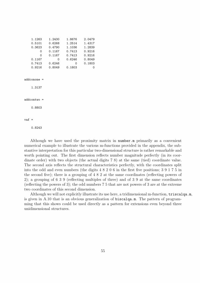
1.1263 1.2430 1.8676 2.04790.5101 0.6268 1.2514 1.43170.3623 0.4790 1.1036 1.2839

0 0.1167 0.7413 0.92160 0.1167 0.7413 0.9216

0.1167 0 0.6246 0.80490.7413 0.6246 0 0.18030.9216 0.8049 0.1803 0

addconone =

1.3137

addcontwo =

0.8803

vaf =

0.8243

Although we have used the proximity matrix in number.m primarily as a convenientnumerical example to illustrate the various m-functions provided in the appendix, the sub-stantive interpretation for this particular two-dimensional structure is rather remarkable andworth pointing out. The first dimension reflects number magnitude perfectly (in its coor-dinate order) with two objects (the actual digits 7 8) at the same (tied) coordinate value.The second axis reflects the structural characteristics perfectly, with the coordinates splitinto the odd and even numbers (the digits 4 8 2 0 6 in the first five positions; 3 9 1 7 5 inthe second five); there is a grouping of 4 8 2 at the same coordinates (reflecting powers of2); a grouping of 6 3 9 (reflecting multiples of three) and of 3 9 at the same coordinates(reflecting the powers of 3); the odd numbers 7 5 that are not powers of 3 are at the extremetwo coordinates of this second dimension.

Although we will not explicitly illustrate its use here, a tridimensional m-function, triscalqa.m,is given in A.10 that is an obvious generalization of biscalqa.m. The pattern of program-ming that this shows could be used directly as a pattern for extensions even beyond threeunidimensional structures.

55

1.2.3 Incorporating Monotonic Transformation of a Proximity Ma-trix in Fitting Multiple Unidimensional Scales: L2 Non-metric Multidimensional Scaling in the City-Block Metric

As a direct extension of the m-function biscalqa.m discussed in the last section, AppendixA.11 gives bimonscalqa.m which provides an optimal monotonic transformation (by incor-porating the use of proxmon.m) of the original proximity matrix given as input in additionto the later’s bidimensional scaling. To prevent degeneracy, the sum-of-squares value for theinitial input proximity matrix is maintained in the optimally transformed proximities; theoverall strategy is iterative with termination again dependent on a change in the variance-accounted-for being less than 1.0e-005. The usage syntax is almost identical to that ofbiscalqa.m except for the inclusion of the monotonically transformed proximity matrixMONPROX as an output matrix:

[ ... monprox] = bimonscalqa( ... )

The ellipses indicate that the same items should be used as in biscalqa.m. If bimonscalqawould have been used in the numerical example of the previous section, the same results givenwould have been provided initially plus the results for the optimally transformed proximitymatrix. We give this additional output below, which shows that the incorporation of anoptimal monotonic transformation provides an increase in the VAF from .8243 to .9362; theorderings on the two dimensions remain the same as well as the nice substantive explanationof the previous section.

outpermone =

Columns 1 through 8

10 8 9 7 6 5 4 3


2 1

outpermtwo =

Columns 1 through 8

6 8 2 4 10 7 1 3


56

5 9

coordone =

-1.6247

-1.1342

-1.1342

-0.5857

-0.1216

-0.0775

0.3565

0.6409

1.3290

2.3514

coordtwo =

-1.0035

-0.8467

-0.3480

-0.3242

-0.3242

0.1196

0.3891

0.7793

0.7793

0.7793

fitone =

Columns 1 through 5

0 0.4906 0.4906 1.0390 1.5032

0.4906 0 0 0.5484 1.0126

0.4906 0 0 0.5484 1.0126

1.0390 0.5484 0.5484 0 0.4642

1.5032 1.0126 1.0126 0.4642 0

1.5473 1.0567 1.0567 0.5083 0.0441

57

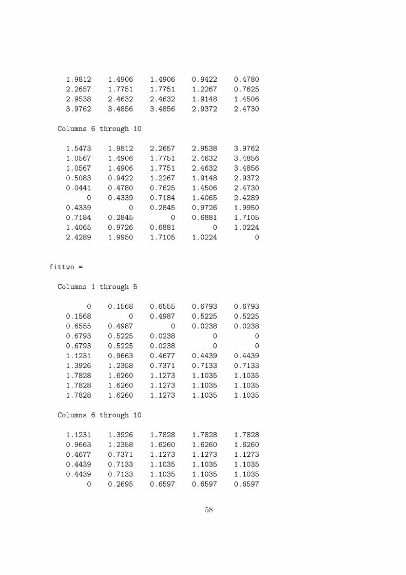
1.9812 1.4906 1.4906 0.9422 0.4780

2.2657 1.7751 1.7751 1.2267 0.7625

2.9538 2.4632 2.4632 1.9148 1.4506

3.9762 3.4856 3.4856 2.9372 2.4730


1.5473 1.9812 2.2657 2.9538 3.9762

1.0567 1.4906 1.7751 2.4632 3.4856

1.0567 1.4906 1.7751 2.4632 3.4856

0.5083 0.9422 1.2267 1.9148 2.9372

0.0441 0.4780 0.7625 1.4506 2.4730

0 0.4339 0.7184 1.4065 2.4289

0.4339 0 0.2845 0.9726 1.9950

0.7184 0.2845 0 0.6881 1.7105

1.4065 0.9726 0.6881 0 1.0224

2.4289 1.9950 1.7105 1.0224 0

fittwo =

Columns 1 through 5

0 0.1568 0.6555 0.6793 0.6793

0.1568 0 0.4987 0.5225 0.5225

0.6555 0.4987 0 0.0238 0.0238

0.6793 0.5225 0.0238 0 0

0.6793 0.5225 0.0238 0 0

1.1231 0.9663 0.4677 0.4439 0.4439

1.3926 1.2358 0.7371 0.7133 0.7133

1.7828 1.6260 1.1273 1.1035 1.1035

1.7828 1.6260 1.1273 1.1035 1.1035

1.7828 1.6260 1.1273 1.1035 1.1035


1.1231 1.3926 1.7828 1.7828 1.7828

0.9663 1.2358 1.6260 1.6260 1.6260

0.4677 0.7371 1.1273 1.1273 1.1273

0.4439 0.7133 1.1035 1.1035 1.1035

0.4439 0.7133 1.1035 1.1035 1.1035

0 0.2695 0.6597 0.6597 0.6597

58

0.2695 0 0.3902 0.3902 0.3902

0.6597 0.3902 0 0.0000 0

0.6597 0.3902 0.0000 0 0

0.6597 0.3902 0 0 0

addconone =

1.4394

addcontwo =

0.7922

vaf =

0.9362

monprox =

Columns 1 through 5

0 -0.7387 -0.1667 0.5067 0.5067

-0.7387 0 -0.8218 -0.8218 0.5067

-0.1667 -0.8218 0 -0.8218 -1.6174

0.5067 -0.8218 -0.8218 0 -0.7387

0.5067 0.5067 -1.6174 -0.7387 0

1.4791 -0.1667 0.5067 -0.7387 -0.7387

1.0321 0.5067 -0.7387 -0.8218 -0.8218

2.6590 0.5067 1.0321 -0.1667 0.5067

1.7609 1.0321 -0.8218 1.0321 -1.2541

2.6231 0.5067 1.4791 -0.8218 0.5067


1.4791 1.0321 2.6590 1.7609 2.6231

-0.1667 0.5067 0.5067 1.0321 0.5067

0.5067 -0.7387 1.0321 -0.8218 1.4791

-0.7387 -0.8218 -0.1667 1.0321 -0.8218

59

-0.7387 -0.8218 0.5067 -1.2541 0.5067

0 -0.8218 -0.8218 0.5067 -0.0534

-0.8218 0 -0.7387 -0.8218 -0.8218

-0.8218 -0.7387 0 -0.7387 -0.7387

0.5067 -0.8218 -0.7387 0 -0.8218

-0.0534 -0.8218 -0.7387 -0.8218 0

Although we will not provide an example of its use here, Appendix A.12 gives trimonscalqa.m,which extends triscalqa.m (listed in A.10) to include an optimal monotonic transformationof whatever is given as the original input proximity matrix.

60

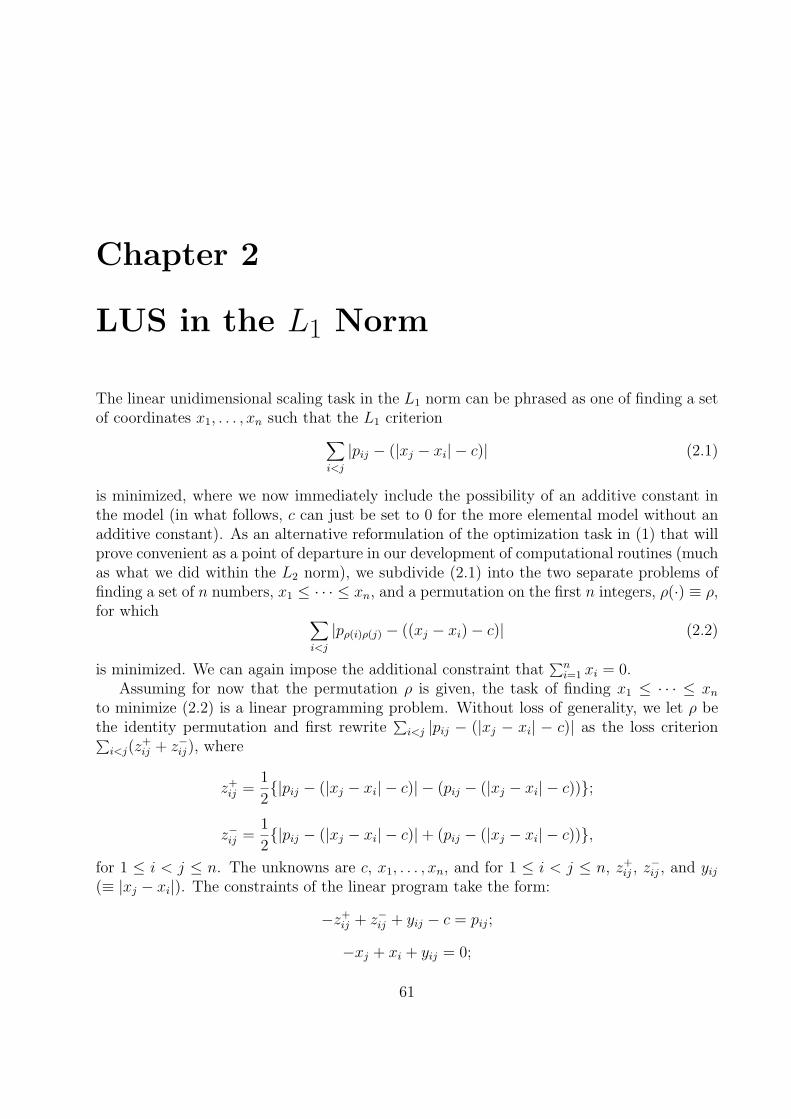
Chapter 2

LUS in the L1 Norm

The linear unidimensional scaling task in the L1 norm can be phrased as one of finding a setof coordinates x1, . . . , xn such that the L1 criterion∑

i<j

|pij − (|xj − xi| − c)| (2.1)

is minimized, where we now immediately include the possibility of an additive constant inthe model (in what follows, c can just be set to 0 for the more elemental model without anadditive constant). As an alternative reformulation of the optimization task in (1) that willprove convenient as a point of departure in our development of computational routines (muchas what we did within the L2 norm), we subdivide (2.1) into the two separate problems offinding a set of n numbers, x1 ≤ · · · ≤ xn, and a permutation on the first n integers, ρ(·) ≡ ρ,for which ∑

i<j

|pρ(i)ρ(j) − ((xj − xi)− c)| (2.2)

is minimized. We can again impose the additional constraint that∑n

i=1 xi = 0.Assuming for now that the permutation ρ is given, the task of finding x1 ≤ · · · ≤ xn

to minimize (2.2) is a linear programming problem. Without loss of generality, we let ρ bethe identity permutation and first rewrite

∑i<j |pij − (|xj − xi| − c)| as the loss criterion∑

i<j(z+ij + z−ij), where

z+ij =

1

2|pij − (|xj − xi| − c)| − (pij − (|xj − xi| − c));

z−ij =1

2|pij − (|xj − xi| − c)|+ (pij − (|xj − xi| − c)),

for 1 ≤ i < j ≤ n. The unknowns are c, x1, . . . , xn, and for 1 ≤ i < j ≤ n, z+ij , z−ij , and yij

(≡ |xj − xi|). The constraints of the linear program take the form:

−z+ij + z−ij + yij − c = pij;

−xj + xi + yij = 0;

61

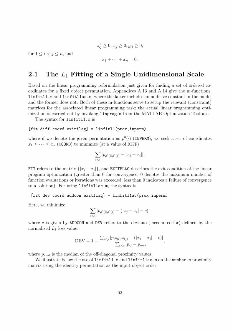
z+ij ≥ 0, z−ij ≥ 0, yij ≥ 0,

for 1 ≤ i < j ≤ n, andx1 + · · ·+ xn = 0.

2.1 The L1 Fitting of a Single Unidimensional Scale

Based on the linear programming reformulation just given for finding a set of ordered co-ordinates for a fixed object permutation, Appendices A.13 and A.14 give the m-functions,linfitl1.m and linfitl1ac.m, where the latter includes an additive constant in the modeland the former does not. Both of these m-functions serve to setup the relevant (constraint)matrices for the associated linear programming task; the actual linear programming opti-mization is carried out by invoking linprog.m from the MATLAB Optimization Toolbox.

The syntax for linfitl1.m is

[fit diff coord exitflag] = linfitl1(prox,inperm)

where if we denote the given permutation as ρ0(·) (INPERM), we seek a set of coordinatesx1 ≤ · · · ≤ xn (COORD) to minimize (at a value of DIFF)∑

i<j

|pρ0(i)ρ0(j) − |xj − xi||;

FIT refers to the matrix |xj − xi|, and EXITFLAG describes the exit condition of the linearprogram optimization (greater than 0 for convergence; 0 denotes the maximum number offunction evaluations or iterations was exceeded; less than 0 indicates a failure of convergenceto a solution). For using linfitl1ac.m, the syntax is

[fit dev coord addcon exitflag] = linfitl1ac(prox,inperm)

Here, we minimize ∑i<j

|pρ0(i)ρ0(j) − (|xj − xi| − c)|

where c is given by ADDCON and DEV refers to the deviance(-accounted-for) defined by thenormalized L1 loss value:

DEV = 1−∑

i<j |pρ0(i)ρ0(j) − (|xj − xi| − c)|∑i<j |pij − pmed|

,

where pmed is the median of the off-diagonal proximity values.We illustrate below the use of linfitl1.m and linfitl1ac.m on the number.m proximity

matrix using the identity permutation as the input object order.

62

load number.dat

inperm = 1:10

inperm =

1 2 3 4 5 6 7 8 9 10

[fit diff coord exitflag] = linfitl1(number,inperm)

Optimization terminated successfully.

fit =

Columns 1 through 6

0 0.3000 0.5840 0.6460 0.6460 0.8040

0.3000 0 0.2840 0.3460 0.3460 0.5040

0.5840 0.2840 0 0.0620 0.0620 0.2200

0.6460 0.3460 0.0620 0 0.0000 0.1580

0.6460 0.3460 0.0620 0.0000 0 0.1580

0.8040 0.5040 0.2200 0.1580 0.1580 0

1.0050 0.7050 0.4210 0.3590 0.3590 0.2010

1.2040 0.9040 0.6200 0.5580 0.5580 0.4000

1.2040 0.9040 0.6200 0.5580 0.5580 0.4000

1.3290 1.0290 0.7450 0.6830 0.6830 0.5250


1.0050 1.2040 1.2040 1.3290

0.7050 0.9040 0.9040 1.0290

0.4210 0.6200 0.6200 0.7450

0.3590 0.5580 0.5580 0.6830

0.3590 0.5580 0.5580 0.6830

0.2010 0.4000 0.4000 0.5250

0 0.1990 0.1990 0.3240

0.1990 0 0.0000 0.1250

0.1990 0.0000 0 0.1250

0.3240 0.1250 0.1250 0

diff =

63

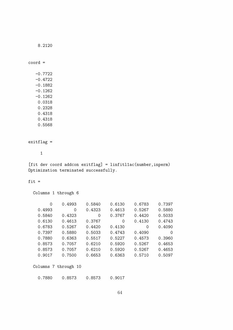
8.2120

coord =

-0.7722

-0.4722

-0.1882

-0.1262

-0.1262

0.0318

0.2328

0.4318

0.4318

0.5568

exitflag =

1

[fit dev coord addcon exitflag] = linfitl1ac(number,inperm)

Optimization terminated successfully.

fit =

Columns 1 through 6

0 0.4993 0.5840 0.6130 0.6783 0.7397

0.4993 0 0.4323 0.4613 0.5267 0.5880

0.5840 0.4323 0 0.3767 0.4420 0.5033

0.6130 0.4613 0.3767 0 0.4130 0.4743

0.6783 0.5267 0.4420 0.4130 0 0.4090

0.7397 0.5880 0.5033 0.4743 0.4090 0

0.7880 0.6363 0.5517 0.5227 0.4573 0.3960

0.8573 0.7057 0.6210 0.5920 0.5267 0.4653

0.8573 0.7057 0.6210 0.5920 0.5267 0.4653

0.9017 0.7500 0.6653 0.6363 0.5710 0.5097


0.7880 0.8573 0.8573 0.9017

64

0.6363 0.7057 0.7057 0.7500

0.5517 0.6210 0.6210 0.6653

0.5227 0.5920 0.5920 0.6363

0.4573 0.5267 0.5267 0.5710

0.3960 0.4653 0.4653 0.5097

0 0.4170 0.4170 0.4613

0.4170 0 0.3477 0.3920

0.4170 0.3477 0 0.3920

0.4613 0.3920 0.3920 0

dev =

0.4252

coord =

-0.3390

-0.1873

-0.1026

-0.0736

-0.0083

0.0530

0.1014

0.1707

0.1707

0.2150

addcon =

-0.3477

exitflag =

1

65

2.1.1 Iterative Linear Programming

Given the availability of the two linear programming based m-functions (discussed in theprevious Section 2.1) for fitting given unidimensional scales defined by specific input objectpermutations, it is possible to imbed these two routines in a search strategy for actuallyfinding the (at least hopefully) best such permutations in the first place. This imbeddingis analogous to adopting iterative quadratic assignment in uniscalqa.m (of Section 1.1.2)and attempting to locate good unidimensional scalings in the L2 norm. Here, we have aniterative use of linear programming in uniscallp.m (in A.15) and uniscallpac.m (in A.16)to identifying the good unidimensional scales in the L1 norm, without and with, respectively,an additive constant in the fitted model. The usage syntax of both m-functions are as follows:

[outperm coord diff fit] = uniscallp(prox,inperm)

[outperm coord dev fit addcon] = uniscallpac(prox,inperm)

Both m-functions begin with a given object ordering (INPERM) and evaluate the effect ofpairwise object interchanges on the current permutation carried forward to that point. If anobject interchange is identified that improves the L1 loss value, that interchange is made andthe changed permutation becomes the current one. When no pairwise object interchangecan reduce DIFF in uniscallp.m, or increase DEV in uniscallpac.m over its current value,that ending permutation is provided as OUTPERM along with its coordinates (COORD) and thematrix FIT (the absolute differences of the ordered coordinates). In uniscallpac.m, theadditive constant (ADDCON) is also given.

The numerical example that follows on our number.dat proximity matrix, initialize boththe m-functions with the identity permutation (1:10). From other random starts that wehave tried in addition to this very rational starting permutation, the resulting scales we givebelow are (almost undoubtedly) L1 norm optimal. We might note that the (optimal) objectorderings differ depending on whether or not an additive constant is included in the model.

[outperm coord diff fit] = uniscallp(number,1:10)

elapsed_time =

1.0611e+003

outperm =

1 2 3 5 4 9 7 6 10 8

coord =

66

-0.7025

-0.3685

-0.2485

-0.1895

-0.0225

0.1185

0.1725

0.2195

0.4685

0.5525

diff =

7.0430

fit =

Columns 1 through 6

0 0.3340 0.4540 0.5130 0.6800 0.8210

0.3340 0 0.1200 0.1790 0.3460 0.4870

0.4540 0.1200 0 0.0590 0.2260 0.3670

0.5130 0.1790 0.0590 0 0.1670 0.3080

0.6800 0.3460 0.2260 0.1670 0 0.1410

0.8210 0.4870 0.3670 0.3080 0.1410 0

0.8750 0.5410 0.4210 0.3620 0.1950 0.0540

0.9220 0.5880 0.4680 0.4090 0.2420 0.1010

1.1710 0.8370 0.7170 0.6580 0.4910 0.3500

1.2550 0.9210 0.8010 0.7420 0.5750 0.4340


0.8750 0.9220 1.1710 1.2550

0.5410 0.5880 0.8370 0.9210

0.4210 0.4680 0.7170 0.8010

0.3620 0.4090 0.6580 0.7420

0.1950 0.2420 0.4910 0.5750

0.0540 0.1010 0.3500 0.4340

0 0.0470 0.2960 0.3800

0.0470 0 0.2490 0.3330

67

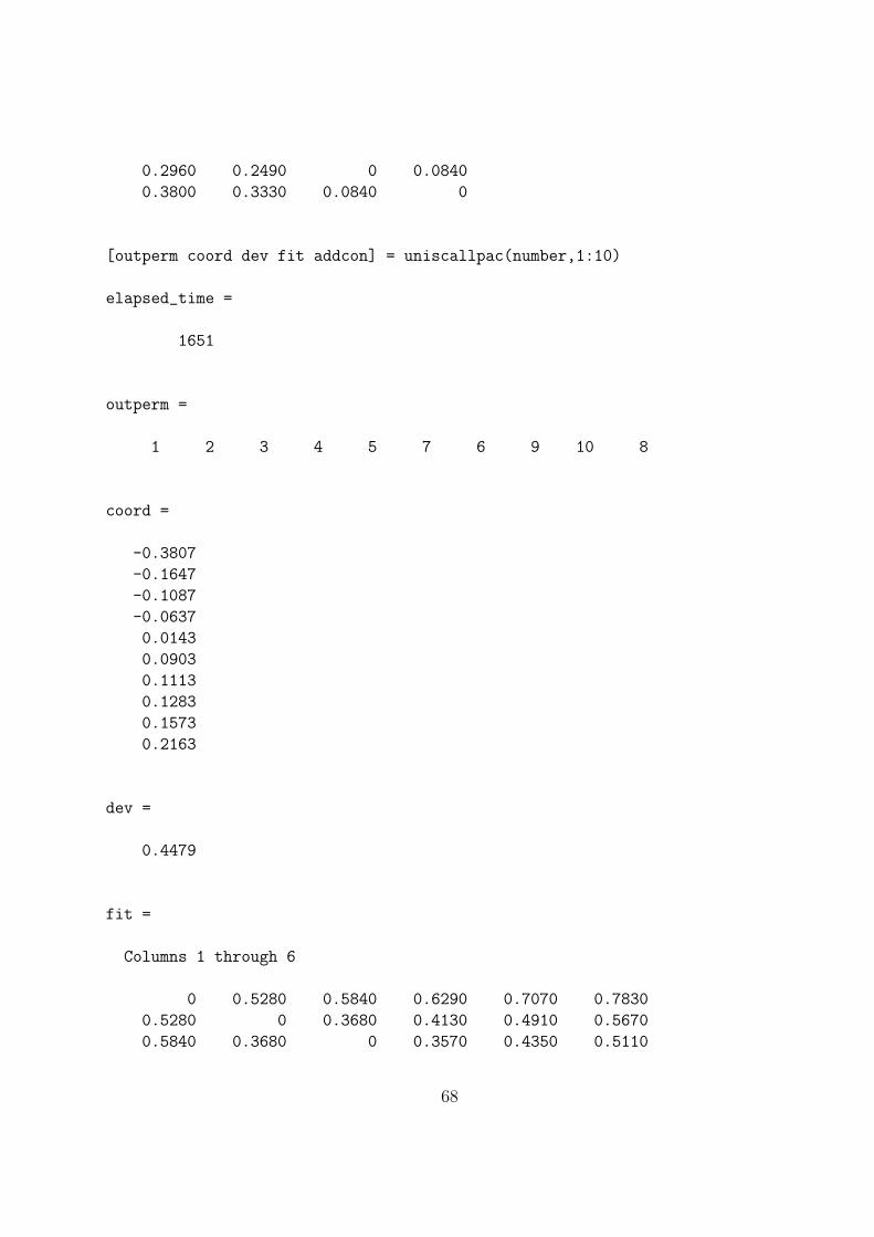
0.2960 0.2490 0 0.0840

0.3800 0.3330 0.0840 0

[outperm coord dev fit addcon] = uniscallpac(number,1:10)

elapsed_time =

1651

outperm =

1 2 3 4 5 7 6 9 10 8

coord =

-0.3807

-0.1647

-0.1087

-0.0637

0.0143

0.0903

0.1113

0.1283

0.1573

0.2163

dev =

0.4479

fit =

Columns 1 through 6

0 0.5280 0.5840 0.6290 0.7070 0.7830

0.5280 0 0.3680 0.4130 0.4910 0.5670

0.5840 0.3680 0 0.3570 0.4350 0.5110

68

0.6290 0.4130 0.3570 0 0.3900 0.4660

0.7070 0.4910 0.4350 0.3900 0 0.3880

0.7830 0.5670 0.5110 0.4660 0.3880 0

0.8040 0.5880 0.5320 0.4870 0.4090 0.3330

0.8210 0.6050 0.5490 0.5040 0.4260 0.3500

0.8500 0.6340 0.5780 0.5330 0.4550 0.3790

0.9090 0.6930 0.6370 0.5920 0.5140 0.4380


0.8040 0.8210 0.8500 0.9090

0.5880 0.6050 0.6340 0.6930

0.5320 0.5490 0.5780 0.6370

0.4870 0.5040 0.5330 0.5920

0.4090 0.4260 0.4550 0.5140

0.3330 0.3500 0.3790 0.4380

0 0.3290 0.3580 0.4170

0.3290 0 0.3410 0.4000

0.3580 0.3410 0 0.3710

0.4170 0.4000 0.3710 0

addcon =

-0.3120

2.2 The L1 Finding and Fitting of Multiple Unidimen-

sional Scales

In analogy to the L2 fitting of multiple unidimensional structures, the use of the L1 normcan again be done by (repetitive) successive residualization, but now with a reliance on them-function, linfitl1ac.m, to fit each separate unidimensional structure with its additiveconstant. The m-function, biscallp.m, given in the Appendix Section A.17 is a two-(orbi-)dimensional scaling strategy for the L1 loss-function∑

i<j

|pij − [|xj1 − xi1| − c1]− [|xj2 − xi2| − c2]|, (2.3)

with syntax (and all variables) similar to biscalqa.m of Section 1.2.2, including a provisionfor the confirmatory fitting of two given input orders (by setting NOPT = 1).

69

In the example given below, the two beginning permutations used were the ones identifiedwith the L2 norm. Compared to the input permutations, there is only one slight change in theinterchange of “3” and “5” in the second output permutation. The final deviance-accounted-for (DEV) of this solution is .6780.

load number.dat

[stannumber,stannumbermult] = proxstd(number,0);

nopt = 1;

inpermone = [10 8 9 7 6 5 4 3 2 1]

inpermone =

10 8 9 7 6 5 4 3 2 1

inpermtwo = [5 9 3 1 7 4 10 2 8 6]

inpermtwo =

5 9 3 1 7 4 10 2 8 6

[outpermone,outpermtwo,coordone,coordtwo,fitone,fittwo,...

addconone,addcontwo,dev] = biscallp(stannumber,inpermone,inpermtwo,nopt)

outpermone =

10 8 9 7 6 5 4 3 2 1

outpermtwo =

5 3 9 1 7 4 10 2 8 6

coordone =

-1.3666

-1.1641

-0.8702

-0.4647

-0.1317

70

-0.0203

0.3600

0.4902

1.1473

2.0201

coordtwo =

-0.9600

-0.9356

-0.8132

-0.1471

-0.0082

0.1366

0.1366

0.5387

0.8147

1.2375

fitone =

Columns 1 through 7

0 -1.0431 -0.7492 -0.3436 -0.0106 0.1008 0.4810

-1.0431 0 -0.9516 -0.5461 -0.2131 -0.1017 0.2786

-0.7492 -0.9516 0 -0.8400 -0.5070 -0.3956 -0.0153

-0.3436 -0.5461 -0.8400 0 -0.9125 -0.8011 -0.4209

-0.0106 -0.2131 -0.5070 -0.9125 0 -1.1341 -0.7539

0.1008 -0.1017 -0.3956 -0.8011 -1.1341 0 -0.8653

0.4810 0.2786 -0.0153 -0.4209 -0.7539 -0.8653 0

0.6113 0.4088 0.1149 -0.2906 -0.6236 -0.7350 -1.1153

1.2684 1.0659 0.7720 0.3664 0.0334 -0.0780 -0.4582

2.1412 1.9388 1.6449 1.2393 0.9063 0.7949 0.4147


0.6113 1.2684 2.1412

0.4088 1.0659 1.9388

0.1149 0.7720 1.6449

-0.2906 0.3664 1.2393

71

-0.6236 0.0334 0.9063

-0.7350 -0.0780 0.7949

-1.1153 -0.4582 0.4147

0 -0.5885 0.2844

-0.5885 0 -0.3727

0.2844 -0.3727 0

fittwo =

Columns 1 through 7

0 -0.8806 -0.7583 -0.0922 0.0468 0.1915 0.1915

-0.8806 0 -0.7827 -0.1166 0.0223 0.1671 0.1671

-0.7583 -0.7827 0 -0.2389 -0.1000 0.0448 0.0448

-0.0922 -0.1166 -0.2389 0 -0.7661 -0.6213 -0.6213

0.0468 0.0223 -0.1000 -0.7661 0 -0.7603 -0.7603

0.1915 0.1671 0.0448 -0.6213 -0.7603 0 -0.9050

0.1915 0.1671 0.0448 -0.6213 -0.7603 -0.9050 0

0.5936 0.5692 0.4469 -0.2192 -0.3582 -0.5029 -0.5029

0.8697 0.8452 0.7229 0.0568 -0.0821 -0.2269 -0.2269

1.2925 1.2680 1.1457 0.4796 0.3407 0.1959 0.1959


0.5936 0.8697 1.2925

0.5692 0.8452 1.2680

0.4469 0.7229 1.1457

-0.2192 0.0568 0.4796

-0.3582 -0.0821 0.3407

-0.5029 -0.2269 0.1959

-0.5029 -0.2269 0.1959

0 -0.6290 -0.2062

-0.6290 0 -0.4822

-0.2062 -0.4822 0

addconone =

1.2455

72

addcontwo =

0.9050

dev =

0.6780

73

Bibliography

[1] Bodewig, E. (1956). Matrix calculus. Amsterdam: North-Holland.

[2] Carroll, J. D. & Pruzansky, S. (1980). Discrete and hybrid scaling models. In E. D.Lantermann & H. Feger (Eds.), Similarity and choice (pp. 108–139). Bern: Hans Huber.

[3] Cheney, W., & Goldstein, A. (1959). Proximity maps for convex sets. Proceedings of theAmerican Mathematical Society. 10, 448–450.

[4] Defays, D. (1978). A short note on a method of seriation. British Journal of Mathemat-ical and Statistical Psychology, 3, 49–53.

[5] de Leeuw, J., & Heiser, W. (1977). Convergence of correction-matrix algorithms formultidimensional scaling. In J. C. Lingoes, E. E. Roskam, & I. Borg (Eds.), Geometricrepresentations of relational data (pp. 735–752). Ann Arbor, MI: Mathesis Press.

[6] Deutsch, F. (1992). The method of alternating orthogonal projections. In S. P. Singh(Ed.), Approximation theory, spline functions, and applications (pp. 105–121). Dor-drecht, The Netherlands: Kluwer.

[7] Dykstra, R. L. (1983). An algorithm for restricted least squares regression. Journal ofthe American Statistical Association, 78, 837–842.

[8] Dykstra, R. L., & Robertson, R. (1982). An algorithm for isotonic regression for two ormore independent variables. Annals of Statistics, 10, 708–718.

[9] Francis, R. L., & White, J. A. (1974). Facility layout and location: An analytical ap-proach. Englewood Cliffs, NJ: Prentice-Hall.

[10] Garey, M. R., & Johnson, D. S. (1979). Computers and intractability. San Francisco:W. H. Freeman.

[11] Guttman, L. (1968). A general nonmetric technique for finding the smallest coordinatespace for a configuration of points. Psychometrika, 33, 469–506.

[12] Heiser, W. J. (1989). The city-block model for three-way multidimensional scaling. In R.Coppi & S. Bolasco (Eds.), Multiway data analysis (pp. 395–404). Amsterdam: North-Holland.

74

[13] Heiser, W. J. (1991). A generalized majorization method for least squares multidimen-sional scaling of pseudodistances that may be negative. Psychometrika, 56, 7–27.

[14] Hubert, L. J., & Arabie, P. (1986). Unidimensional scaling and combinatorial optimiza-tion. In J. de Leeuw, W. Heiser, J. Meulman, & F. Critchely (Eds.), Multidimensionaldata analysis (pp. 181–196). Leiden, The Netherlands: DSWO Press.

[15] Hubert, L. J., & Arabie, P. (1994). The analysis of proximity matrices through sums ofmatrices having (anti-)Robinson forms. British Journal of Mathematical and StatisticalPsychology, 47, 1–40.

[16] Hubert, L. J., & Arabie, P. (1995). Iterative projection strategies for the least-squaresfitting of tree structures to proximity data. British Journal of Mathematical and Statis-tical Psychology, 48, 281–317.

[17] Hubert, L. J., Arabie, P., & Meulman, J. (1997). Linear and circular unidimensionalscaling for symmetric proximity matrices. British Journal of Mathematical and Statis-tical Psychology, 50, 253–284.

[18] Hubert, L. J., Arabie, P., & Meulman, J. (2001). Combinatorial data analysis: Opti-mization by dynamic programming. Philadelphia: SIAM.

[19] Hubert, L. J., & Schultz, J. W. (1976). Quadratic assignment as a general data analysisstrategy. British Journal of Mathematical and Statistical Psychology, 29, 190–241.

[20] Kaczmarz, S. (1937). Angenaherte Auflosung von Systemen linearer Gleichungen. Bul-letin of the Polish Academy of Sciences, A35, 355–357.

[21] Lawler, E. L. (1975). The quadratic assignment problem: A brief review. In R. Roy(Ed.), Combinatorial programming: Methods and applications (pp. 351–360). Dordrecht,The Netherlands: Reidel.

[22] Lau, Kin-nam, Leung, Pui Lam, & Tse, Ka-kit (1998). A nonlinear programming ap-proach to metric unidimensional scaling. Journal of Classification, 15, 3–14.

[23] Pardalos, P. M., & Wolkowicz, H. (Eds.). (1994). Quadratic assignment and relatedproblems. DIMACS Series on Discrete Mathematics and Theoretical Computer Science.Providence, RI: American Mathematical Society.

[24] Pliner, V. (1996). Metric unidimensional scaling and global optimization. Journal ofClassification, 13, 3–18.

[25] Shepard, R. N. (1974). Representation of structure in similarity data: Problems andprospects. Psychometrika, 39, 373–421.

[26] Shepard, R. N., Kilpatric, D. W., & Cunningham, J. P. (1975). The internal represen-tation of numbers. Cognitive Psychology, 7, 82–138.

75

Appendix A

main program files

A.1 uniscaldp.m

function [coord,permut,cumobfun,diff] = uniscaldp(prox)

%UNISCALDP carries out a unidimensional scaling of a symmetric proximity% matrix using dynamic programming.% PROX is the input proximity matrix (with a zero main diagonal and a% dissimilarity interpretation);% COORD is the set of coordinates of the optimal unidimensional scaling% in ascending order;% PERMUT is the order of the objects in the optimal permutation(say,% $\rho^*$);% CUMOBFUN gives the cumulative values of the objective function for% the successive placements of the objects in the optimal permutation:% $\sum_i=1^k (t_i^(\rho^*))^2$ for $k = 1, \ldots, n$;% DIFF is the value of the least-squares loss function for the optimal% coordinates and object permutation.

% Initializations. The vectors VALSTORE and IDXSTORE store the results of% of the recursion for the $(2^n)-1$ nonempty subsets of $S$. The integer% positions in these vectors correspond to subsets whose binary% number equivalents are equal those integer positions.

tic;n = size(prox,1);bigneg = -1.0e+20;nsum = (2^n) - 1;valstore = ones(nsum,1)*bigneg;idxstore = zeros(nsum,1);sub = zeros(n,1);

76

subcomp = zeros(n,1);coord = zeros(n,1);permut = zeros(n,1);cumobfun = zeros(n,1);

% Initializing the recursion for subsets of size 1for i = 1:n

rowsum = 0;for j = 1:n

rowsum = rowsum + prox(i,j);endindex = 2^(i-1);idxstore(index) = i;valstore(index) = rowsum^2;

end

% Carrying out the recursion for subsets of size $k$ from $k = 1$% to $n-1$ by adapting a Fortran subroutine from Nijenhuis and Wilf% (1978, Combinatorial Algorithms, Academic Press, pp. 26--38) on% generating the next k-subset from an n-Set% (and placed in the variable SUB)mtc = 0;for k = 1:(n-1)

nfirst = 0;if(mtc == 0)

m2 = 0;nh = k;for j = 1:nh

sub(k+j-nh) = m2 + j;endif(sub(1) ~= (n-k+1))

mtc = 1;end

end

while (mtc == 1)if(nfirst == 1)

if(m2 < (n-nh))nh = 0;

endnh = nh + 1;m2 = sub(k+1-nh);for j = 1:nh

sub(k+j-nh) = m2 + j;end

77

if(sub(1) ~= (n-k+1))mtc = 1;

elsemtc = 0;

endend

if(nfirst == 0)nfirst = 1;

endindex = 0;

for i = 1:kindex = index + 2^(sub(i)-1);

end

% Generating the complement (SUBCOMP) of the subset indicated in SUBjj = 1;subcomp = zeros(n,1);for i = 1:n

idxcomp = 1;for j = 1:k

if(sub(j) == i)idxcomp = 0;

endendif(idxcomp == 1)

subcomp(jj) = i;jj = jj + 1;

endend

% Trying to add objects from SUBCOMP one at a time to the end of% SUB to see if better placements can be found

nk = n - k;for jj = 1:nk

jone = subcomp(jj);sum = 0.0;for i = 1:k

ione = sub(i);sum = sum + prox(jone,ione);

endfor i = 1:nk

ione = subcomp(i);if(ione ~= jone)

sum = sum - prox(jone,ione);

78

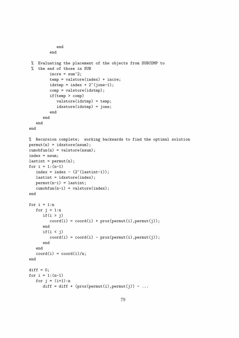
endend

% Evaluating the placement of the objects from SUBCOMP to% the end of those in SUB

incre = sum^2;temp = valstore(index) + incre;idxtmp = index + 2^(jone-1);comp = valstore(idxtmp);if(temp > comp)

valstore(idxtmp) = temp;idxstore(idxtmp) = jone;

endend

endend

% Recursion complete; working backwards to find the optimal solutionpermut(n) = idxstore(nsum);cumobfun(n) = valstore(nsum);index = nsum;lastint = permut(n);for i = 1:(n-1)

index = index - (2^(lastint-1));lastint = idxstore(index);permut(n-i) = lastint;cumobfun(n-i) = valstore(index);

end

for i = 1:nfor j = 1:n

if(i > j)coord(i) = coord(i) + prox(permut(i),permut(j));

endif(i < j)

coord(i) = coord(i) - prox(permut(i),permut(j));end

endcoord(i) = coord(i)/n;

end

diff = 0;for i = 1:(n-1)

for j = (i+1):ndiff = diff + (prox(permut(i),permut(j)) - ...

79

abs(coord(i) - coord(j)))^2;end

endtoc

A.2 uniscaldpf.m

function [coord,permut,cumobfun,diff] = uniscaldpf(prox)

tic;n = size(prox,1);bigneg = -1.0e+20;nsum = (2^n) - 1;sub = zeros(n,1);subcomp = zeros(n,1);coord = zeros(n,1);permut = zeros(n,1);cumobfun = zeros(n,1);

[valstore vidxstore] = uscalfor(prox);

permut(n) = vidxstore(nsum);cumobfun(n) = valstore(nsum);index = nsum;lastint = permut(n);for i = 1:(n-1)

index = index - (2^(lastint-1));lastint = vidxstore(index);permut(n-i) = lastint;cumobfun(n-i) = valstore(index);

end


if(i > j)coord(i) = coord(i) + prox(permut(i),permut(j));

endif(i < j)

coord(i) = coord(i) - prox(permut(i),permut(j));end


80

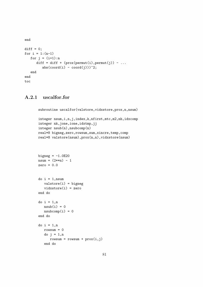
end

diff = 0;for i = 1:(n-1)

for j = (i+1):ndiff = diff + (prox(permut(i),permut(j)) - ...


endtoc

A.2.1 uscalfor.for

subroutine uscalfor(valstore,vidxstore,prox,n,nsum)

integer nsum,i,n,j,index,k,nfirst,mtc,m2,nh,idxcompinteger nk,jone,ione,idxtmp,jjinteger nsub(n),nsubcomp(n)real*8 bigneg,zero,rowsum,sum,xincre,temp,compreal*8 valstore(nsum),prox(n,n),vidxstore(nsum)

bigneg = -1.0E20nsum = (2**n) - 1zero = 0.0

do i = 1,nsumvalstore(i) = bignegvidxstore(i) = zero

end do

do i = 1,nnsub(i) = 0nsubcomp(i) = 0

end do

do i = 1,nrowsum = 0do j = 1,n

rowsum = rowsum + prox(i,j)end do

81

index = 2**(i-1)valstore(index) = rowsum**2vidxstore(index) = i

end do

mtc = 0

do k = 1,n-1nfirst = 0

if(mtc.eq.0) thenm2 = 0nh = kdo j = 1,nh

nsub(k+j-nh) = m2 + jend doif(nsub(1).ne.(n-k+1)) then

mtc = 1end if

end if

do while(mtc.eq.1)if(nfirst.eq.1) then

if(m2.lt.(n-nh)) thennh = 0

end ifnh = nh + 1m2 = nsub(k+1-nh)do j = 1,nh

nsub(k+j-nh) = m2 + jend doif(nsub(1).ne.(n-k+1)) then

mtc = 1else

mtc = 0end if

end if

if(nfirst.eq.0) thennfirst = 1

end ifindex = 0

do i = 1,kindex = index + 2**(nsub(i)-1)

end do

82

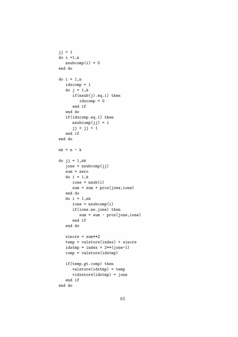
jj = 1do i =1,n

nsubcomp(i) = 0end do

do i = 1,nidxcomp = 1do j = 1,k

if(nsub(j).eq.i) thenidxcomp = 0

end ifend doif(idxcomp.eq.1) then

nsubcomp(jj) = ijj = jj + 1

end ifend do

nk = n - k

do jj = 1,nkjone = nsubcomp(jj)sum = zerodo i = 1,k

ione = nsub(i)sum = sum + prox(jone,ione)

end dodo i = 1,nk

ione = nsubcomp(i)if(ione.ne.jone) then

sum = sum - prox(jone,ione)end if

end do

xincre = sum**2temp = valstore(index) + xincreidxtmp = index + 2**(jone-1)comp = valstore(idxtmp)

if(temp.gt.comp) thenvalstore(idxtmp) = tempvidxstore(idxtmp) = jone

end ifend do

83

end doend do

returnend

A.2.2 uscalforgw.for

subroutine mexFunction(nlhs,plhs,nrhs,prhs)

integer plhs(*),prhs(*)integer mxCreateFull,mxGetPrinteger mxGetM,mxGetN,m,n,nsize,nsuminteger valstore_pr,vidxstore_pr,prox_printeger nlhs,nrhsreal*8 valstore(2**25),prox(25*25),vidxstore(2**25)

m = mxGetM(prhs(1))n = mxGetN(prhs(1))nsize = m*nnsum = (2**n) - 1if(n.gt.25) then

call mexErrMsgTxt(’n must be <= 25’)end if

plhs(1) = mxCreateFull(nsum,1,0)plhs(2) = mxCreateFull(nsum,1,0)prox_pr = mxGetPr(prhs(1))valstore_pr = mxGetPr(plhs(1))vidxstore_pr = mxGetPr(plhs(2))

call mxCopyPtrToReal8(prox_pr,prox,nsize)call uscalfor(valstore,vidxstore,prox,n,nsum)call mxCopyReal8ToPtr(valstore,valstore_pr,nsum)call mxCopyReal8ToPtr(vidxstore,vidxstore_pr,nsum)

return

end

84

A.3 uniscalqa.m

function [outperm, rawindex, allperms, index, coord, diff] = ...uniscalqa(prox, targ, inperm, kblock)

%UNISCALQA carries out a unidimensional scaling of a symmetric proximity% matrix using iterative quadratic assignment.% PROX is the input proximity matrix (with a zero main diagonal and a% dissimilarity interpretation);% TARG is the input target matrix (usually with a zero main diagonal and% with a dissimilarity interpretation representing equally-spaced locations% along a continuum);% INPERM is the input beginning permutation (a permuation of the first $n$ integers).% OUTPERM is the final permutation of PROX with the cross-product index RAWINDEX% with respect to TARG redefined as $ = \abs(coord(i) - coord(j))\$;% ALLPERMS is a cell array containing INDEX entries corresponding to all the% permutations identified in the optimization from ALLPERMS1 = INPERM to% ALLPERMSINDEX = OUTPERM.% The insertion and rotation routines use from 1 to KBLOCK% (which is less than or equal to $n-1$)% consecutive objects in% the permutation defining the row and column order of the data matrix.% COORD is the set of coordinates of the unidimensional scaling% in ascending order;% DIFF is the value of the least-squares loss function for the% coordinates and object permutation.

tic;n = size(prox,1);outperm = inperm;index = 1;allpermsindex = inperm;begindex = sum(sum(prox(inperm,inperm).*targ));coord = zeros(n,1);

prevperm = inperm;nprevperm = 1;

while (nprevperm == 1)nprevperm = 0;

nchange = 1;

while (nchange == 1)

85

nchange=0;

for k = 1:(n-1)for j = (k+1):n

intrperm = outperm;

intrperm(k) = outperm(j);intrperm(j) = outperm(k);

tryindex = sum(sum(prox(intrperm,intrperm).*targ));

if(tryindex > (begindex + 1.0e-008))nchange = 1;begindex = tryindex;outperm = intrperm;index = index + 1;allpermsindex = intrperm;

end

endend

for k = 1:kblockfor insertpt = 1:(n+1)

for nlimlow = 1:(n+1-k)

intrperm = outperm;

if (nlimlow > insertpt)

jtwo = 0;for j = insertpt:(insertpt+k-1)

intrperm(j) =outperm(nlimlow+jtwo);jtwo = jtwo + 1;

end

jone = 0;for j = (insertpt+k):(nlimlow+k-1);

intrperm(j) = outperm(insertpt+jone);jone = jone + 1;

end

86

elseif ((nlimlow+k) < insertpt)

jtwo = 0;for j = (insertpt-k):(insertpt-1)

intrperm(j) = outperm(nlimlow+jtwo);jtwo = jtwo + 1;

end

jone = 0;for j = nlimlow:(insertpt-k-1)

intrperm(j) = outperm(nlimlow+k+jone);jone = jone + 1;

end

else

end


if(tryindex > (begindex + 1.0e-008))nchange = 1;begindex = tryindex;outperm = intrperm;index = index +1;allpermsindex = intrperm;

end

endend

end

if (kblock > 1)

for k = 2:kblockfor nlimlow = 1:(n+1-k)

intrperm = outperm;

for j = 1:kintrperm(nlimlow+j-1) = outperm(nlimlow+k-j);

end


87


end

endend

end

end

rawindex = begindex;if(any(prevperm - outperm) == 1)

nprevperm = 1;prevperm = outperm;

end

coord = zeros(n,1);


if(i > j)coord(i) = coord(i) + prox(outperm(i),outperm(j));

endif(i < j)

coord(i) = coord(i) - prox(outperm(i),outperm(j));end


end

diff = 0;for i = 1:(n-1)

for j = (i+1):ndiff = diff + (prox(outperm(i),outperm(j)) - ...


end


88

targ(i,j) = abs(coord(i) - coord(j));end

end

begindex = sum(sum(prox(outperm,outperm).*targ));

end

toc

A.4 guttorder.m

function [gcoordsort, gperm] = ...guttorder(prox,inperm)

%GUTTORDER carries out a unidimensional scaling of a symmetric proximity% matrix using Guttman’s updating algorithm.% PROX is the input proximity matrix (with a zero main diagonal and a% dissimilarity interpretation);% INPERM is an input permutation of the first $n$ integers;% GCOORDSORT are the coordinates ordered from most negative to most positive;% GPERM is the object permutation that indicates which objects are at which of the% ordered coordinates in GCOORDSORT.

n = size(prox,1);gpermprev = inperm;gcoord = zeros(n,1);gcoordprev = zeros(n,1);


if(inperm(j) == i)gcoordprev(i) = j;

endend

end

for i = 1:n

89

for j = 1:ngcoord(i) = gcoord(i) + (prox(i,j)*sign(gcoordprev(i) - ...

gcoordprev(j)))/n;end

end

gperm = 1:n;gcoordsort = gcoord;

for i = 1:(n-1)for j = (i+1):n

if(gcoordsort(i) > gcoordsort(j))tempcoord = gcoordsort(i);gcoordsort(i) = gcoordsort(j);gcoordsort(j) = tempcoord;tempperm = gperm(i);gperm(i) = gperm(j);gperm(j) = tempperm;

endend

end

while(any(gpermprev - gperm) == 1)gcoordprev = gcoord;gpermprev = gperm;gcoord = zeros(n,1);for i = 1:n



end


for i = 1:(n-1)for j = (i+1):n

if(gcoordsort(i) > gcoordsort(j))tempcoord = gcoordsort(i);gcoordsort(i) = gcoordsort(j);gcoordsort(j) = tempcoord;

90

tempperm = gperm(i);gperm(i) = gperm(j);gperm(j) = tempperm;

endend

end

end

A.5 plinorder.m

function [pcoordsort, pperm, gcoordsort, gperm, gdiff, pdiff] = ...plinorder(prox,inperm)

%PLINORDER carries out a unidimensional scaling of a symmetric proximity% matrix using Pliner smoothing function in Guttman’s updating algorithm.% PROX is the input proximity matrix (with a zero main diagonal and a% dissimilarity interpretation);% INPERM is an input permutation of the first $n$ integers;% GCOORDSORT are the coordinates from the Guttman update ordered from most negative to most positive;% GPERM is the object permutation that indicates which objects are at which of the% ordered coordinates in GCOORDSORT;% PCOORDSORT are the coordinates from the Pliner smoother of the Guttman update ordered from most% negative to most positive;% PPERM is the object permutation that indicates which objects are at which of the ordered% coordinates in PCOORDSORT;% GDIFF is the value of the least-squares loss function for the% coordinates and object permutation obtained from the Guttman update;% PDIFF is the value of the least-squares loss function for the coordinates% and object permutation obtained from the Pliner smoothing procedure.

n = size(prox,1);gpermprev = inperm;gcoord = zeros(n,1);gcoordprev = zeros(n,1);


if(inperm(j) == i)gcoordprev(i) = j;

91

endend

end


gcoord(i) = gcoord(i) + (prox(i,j)*sign(gcoordprev(i) - ...gcoordprev(j)))/n;

endend


for i = 1:(n-1)for j = (i+1):n

if(gcoordsort(i) > gcoordsort(j))tempcoord = gcoordsort(i);gcoordsort(i) = gcoordsort(j);gcoordsort(j) = tempcoord;tempperm = gperm(i);gperm(i) = gperm(j);gperm(j) = tempperm;

endend

endgpermprev = randperm(n);

while(any(gpermprev - gperm) == 1)gcoordprev = gcoord;gpermprev = gperm;gcoord = zeros(n,1);for i = 1:n



end


for i = 1:(n-1)

92

for j = (i+1):nif(gcoordsort(i) > gcoordsort(j))

tempcoord = gcoordsort(i);gcoordsort(i) = gcoordsort(j);gcoordsort(j) = tempcoord;tempperm = gperm(i);gperm(i) = gperm(j);gperm(j) = tempperm;

endend

end

gdiff = 0;for i = 1:n

for j = 1:ngdiff = gdiff + (prox(i,j) - abs(gcoord(i) - gcoord(j)))^2;

endend

end

ep = 2*(max(sum(prox))/n);pperm = gperm;pcoord = gcoord;

for k = 2:100

ppermprev = randperm(n);

while(any(ppermprev - pperm) == 1)

pcoordprev = pcoord;ppermprev = pperm;

pcoord = zeros(n,1);for i = 1:n

for j = 1:nabst = abs(pcoordprev(i) - pcoordprev(j));if(abst < ep)

factor = ((pcoordprev(i) - pcoordprev(j))/ep)* ...(2 - (abst/ep));

endif(abst >= ep)

factor = sign(pcoordprev(i) - pcoordprev(j));

93

endpcoord(i) = pcoord(i) + (prox(i,j)*factor)/n;

endend

pperm = 1:n;pcoordsort = pcoord;

for i = 1:(n-1)for j = (i+1):n

if(pcoordsort(i) > pcoordsort(j))tempcoord = pcoordsort(i);pcoordsort(i) = pcoordsort(j);pcoordsort(j) = tempcoord;tempperm = pperm(i);pperm(i) = pperm(j);pperm(j) = tempperm;

endend

end

pdiff = 0;for i = 1:n

for j = 1:npdiff = pdiff + (prox(i,j) - abs(pcoord(i) - pcoord(j)))^2;

endend

endep = ep*(100 - k +1)/100;

endgdiff = .5*gdiff;pdiff = .5*pdiff;

A.6 unifitl2nlp.m

function [startcoord, begval, outcoord, endval, exitflag] = ...

94

unifitl2nlp(prox,inperm)

%UNIFITL2NLP carries out a unidimensional scaling of a symmetric proximity% matrix using the l2 norm and the nonlinear programming refomulation of% Lau, Leung, and Tse.% PROX is the input proximity matrix (with a zero main diagonal and a% dissimilarity interpretation);% INPERM is the input permutation of the first $n$ integers which is used to% obtain the starting coordinates (STARTCOORD) and the initial least squares% loss value (BEGVAL);% OUTCOORD are the ending coordinates values having the final least squares loss% value of ENDVAL;% EXITFLAG indicates the success of the optimization ( > 0 indicates convergence;% 0 indicates that the maximum number of function evaluations or iterations were% reached; and < 0 denotes nonconvergence).

n = size(prox,1);outcoord = zeros(n,1);tmpcoord = zeros(n,1);coord = zeros(n,1);proxmat = prox(inperm,inperm);


if(i>j)tmpcoord(i) = tmpcoord(i) + proxmat(i,j);

endif(i<j)

tmpcoord(i) = tmpcoord(i) - proxmat(i,j);end

end

tmpcoord(i) = tmpcoord(i)/n;

end


if(inperm(i) == j)coord(j) = tmpcoord(i);

endend

end

nch2 = n*(n-1)/2;

95

xlength = (4*nch2) + n;xstart = zeros(xlength,1);

for i = 1:nxstart(i) = coord(i);

end

index = n;for i = 2:n

for j = 1:(i-1)index = index + 1;xstart(index) = prox(i,j) - coord(i) + coord(j);xstart(index+nch2) = prox(i,j) - coord(j) + coord(i);if(coord(i) > coord(j))

xstart(index+2*nch2) = 1;endif(coord(i) < coord(j))

xstart(index+3*nch2) = 1;end

endend

aequal = zeros(3*nch2+1,xlength);

index = 0;for i = 2:n

for j = 1:(i-1)index = index + 1;aequal(index,i) = 1;aequal(index,j) = -1;aequal(index,index+n) = 1;aequal(index+nch2,i) = -1;aequal(index+nch2,j) = 1;aequal(index+nch2,index+nch2+n) = 1;aequal(index+2*nch2,index+2*nch2+n) = 1;aequal(index+2*nch2,index+3*nch2+n) = 1;

endend

for i = 1:naequal(3*nch2+1,i) = 1;

end

96

bconst = zeros(3*nch2+1,1);


for j = 1:(i-1)index = index + 1;bconst(index) = prox(i,j);bconst(index+nch2) = prox(i,j);bconst(index+2*nch2) = 1;

endend

bconst(3*nch2+1) = 0;

for i = 1:xlengthlbound(i) = -inf;if(i > (n+2*nch2))

lbound(i) = 0;end

end

[xend,fval,exitflag,output] = ...fmincon(’objfunl2’,xstart,[],[],aequal,bconst,lbound,[]);

for i = 1:noutcoord(i) = xend(i);

end

startcoord = coord;begval = objfunl2(xstart);outcoord;endval = objfunl2(xend);

A.6.1 objfunl2.m

function f = objfunl2(x)

97

%OBJFUNL2 provides the objective function evaluations needed for unifitl2nlp.m.

c = length(x);n = round((1 + sqrt(1+8*c))/4);nch2 = n*(n-1)/2;

f = 0;index = n;for i = 2:n

for j = 1:(i-1)index = index + 1;f = f + x(index+2*nch2)*x(index)*x(index) + ...

x(index+3*nch2)*x(index+nch2)*x(index+nch2);end

end

A.7 linfit.m

function [fit, diff, coord] = linfit(prox,inperm)

%LINFIT does a confirmatory fitting of a given unidimensional order using Dykstra’s% (Kaczmarz’s) iterative projection least-squares method.% INPERM is the given order;% FIT is an $n \times n$ matrix that is fitted to PROX(INPERM,INPERM) with% least-squares value DIFF;% COORD gives the ordered coordinates whose absolute differences% could be used to reconstruct FIT.

n=size(prox,1);work = zeros(n*(n-1)*(n-2),1);fit = prox(inperm,inperm);work = zeros(n*(n-1)*(n-2),1);cr = 1.0;

while (cr >= 1.0e-006)

cr = 0.0;index = 0;

for jone = 1:(n-2)for jtwo = (jone+1):(n-1)

for jthree = (jtwo+1):n

98

p1 = fit(jone,jtwo);p2 = fit(jone,jthree);p3 = fit(jtwo,jthree);

fit(jone,jtwo) = fit(jone,jtwo) - work(index+1);fit(jone,jthree) = fit(jone,jthree) - work(index+2);fit(jtwo,jthree) = fit(jtwo,jthree) - work(index+3);

del = (fit(jone,jthree) - fit(jone,jtwo) - ...fit(jtwo,jthree))/3.0;

fit(jone,jthree) = fit(jone,jthree) - del;fit(jone,jtwo) = fit(jone,jtwo) + del;fit(jtwo,jthree) = fit(jtwo,jthree) + del;

work(index+1) = del;work(index+2) = -del;work(index+3) = del;

index = index + 3;

cr = cr + abs(p1-fit(jone,jtwo)) + abs(p2-fit(jone,jthree)) ...+ abs(p3 - fit(jtwo,jthree));

endend

end

for jone = 1:(n-1)for jtwo = (jone+1):n

p1 = fit(jone,jtwo);fit(jone,jtwo) = fit(jone,jtwo) - work(index+1);

if(fit(jone,jtwo) < 0.0)

work(index+1) = -fit(jone,jtwo);fit(jone,jtwo) = 0.0;

else

work(index+1) = 0.0;

end

99

index = index + 1;

cr= cr + abs(p1-fit(jone,jtwo));end

endend


fit(jtwo,jone) = fit(jone,jtwo);

endend

aveprox = sum(sum(prox))/(n*(n-1));


if( i ~= j)proxave(i,j) = aveprox;

elseproxave(i,j) = 0;

endend

end

diff = sum(sum((prox(inperm,inperm) - fit).^2));

% denom = sum(sum((prox(inperm,inperm) - proxave).^2));

denom = sum(sum((prox(inperm,inperm)).^2));

vaf = 1 - (diff/denom);coord = zeros(n,1);


if(i>j)coord(i) = coord(i) + fit(i,j);

endif(i<j)

coord(i) = coord(i) - fit(i,j);

100

endend

coord(i) = coord(i)/n;end

diff = (.5)*diff;

A.8 linfitac.m

function [fit, vaf, coord, addcon] = linfitac(prox,inperm)

%LINFITAC does a confirmatory fitting of a given unidimensional order% using the Dykstra-Kaczmarz iterative projection least-squares method,% but differing from LINFIT.M in including the estimation of an additive% constant.% INPERM is the given order;% FIT is an $n \times n$ matrix that is fitted to PROX(INPERM,INPERM) with% variance-accounted-for VAF;% COORD gives the ordered coordinates whose absolute differences% could be used to reconstruct FIT; ADDCON is the estimated additive constant% that can be interpreted as being added to PROX.

n=size(prox,1);acondiff = 1.0;addcon = 0.0;

while (acondiff >= 1.0e-005)

for i =1:nfor j=1:n

if(i ~= j)fit(i,j) = prox(inperm(i),inperm(j)) + addcon;

elsefit(i,j) = 0.0;

endend

end

101

addconpv = addcon;

work = zeros(n*(n-1)*(n-2),1);cr = 1.0;

while (cr >= 1.0e-006)

cr = 0.0;index = 0;

for jone = 1:(n-2)for jtwo = (jone+1):(n-1)

for jthree = (jtwo+1):n

p1 = fit(jone,jtwo);p2 = fit(jone,jthree);p3 = fit(jtwo,jthree);

fit(jone,jtwo) = fit(jone,jtwo) - work(index+1);fit(jone,jthree) = fit(jone,jthree) - work(index+2);fit(jtwo,jthree) = fit(jtwo,jthree) - work(index+3);

del = (fit(jone,jthree) - fit(jone,jtwo) - ...fit(jtwo,jthree))/3.0;

fit(jone,jthree) = fit(jone,jthree) - del;fit(jone,jtwo) = fit(jone,jtwo) + del;fit(jtwo,jthree) = fit(jtwo,jthree) + del;

work(index+1) = del;work(index+2) = -del;work(index+3) = del;

index = index + 3;

cr = cr + abs(p1-fit(jone,jtwo)) + abs(p2-fit(jone,jthree)) ...+ abs(p3 - fit(jtwo,jthree));

endend

end


102

p1 = fit(jone,jtwo);

fit(jone,jtwo) = fit(jone,jtwo) - work(index+1);

if(fit(jone,jtwo) < 0.0)

work(index+1) = -fit(jone,jtwo);fit(jone,jtwo) = 0.0;

else

work(index+1) = 0.0;

end

index = index + 1;

cr= cr + abs(p1-fit(jone,jtwo));end

endend



endend

addcon = -sum(sum(prox(inperm,inperm) - fit))/(n*(n-1));

acondiff = abs(addcon - addconpv);

end

aveprox = sum(sum(prox))/(n*(n-1));


if( i ~= j)

103

proxave(i,j) = aveprox;fmadd(i,j) = fit(i,j) - addcon;

elseproxave(i,j) = 0;fmadd(i,j) = 0.0;

endend

end

diff = sum(sum((prox(inperm,inperm) - (fmadd)).^2));

denom = sum(sum((prox(inperm,inperm) - proxave).^2));

%denom = sum(sum((prox(inperm,inperm)).^2));

vaf = 1 - (diff/denom);

coord = zeros(n,1);


if(i>j)coord(i) = coord(i) + fit(i,j);

endif(i<j)

coord(i) = coord(i) - fit(i,j);end

end

coord(i) = coord(i)/n;end

A.9 biscalqa.m

function [outpermone,outpermtwo,coordone,coordtwo,fitone,fittwo,addconone,addcontwo,vaf] = ...biscalqa(prox,targone,targtwo,inpermone,inpermtwo,kblock,nopt)

%BISCALQA carries out a bidimensional scaling of a symmetric proximity% matrix using iterative quadratic assignment.% PROX is the input proximity matrix (with a zero main diagonal and a

104

% dissimilarity interpretation);% TARGONE is the input target matrix for the first dimension (usually with% a zero main diagonal and with a dissimilarity interpretation representing% equally-spaced locations along a continuum); TARGTWO is the input target% matrix for the second dimension;% INPERMONE is the input beginning permutation for the first dimension% (a permuation of the first $n$ integers); INPERMTWO is the input beginning% permutation for the second dimension;% the insertion and rotation routines use from 1 to KBLOCK% (which is less than or equal to $n-1$) consecutive objects in% the permutation defining the row and column orders of the data matrix.% NOPT controls the confirmatory or exploratory fitting of the unidimensional% scales; a value of NOPT = 0 will fit in a confirmatory manner the two scales% indicated by INPERMONE and INPERMTWO; a value of NOPT = 1 uses iterative QA% to locate the better permutations to fit;% OUTPERMONE is the final object permutation for the first dimension;% OUTPERMTWO is the final object permutation for the second dimension;% COORDONE is the set of first dimension coordinates in ascending order;% COORDTWO is the set of second dimension coordinates in ascending order;% ADDCONONE is the additive constant for the first dimensional model;% ADDCONTWO is the additive constant for the second dimensional model;% VAF is the variance-accounted-for in PROX by the bidimensional scaling.

tic;n = size(prox,1);outpermone = inpermone;outpermtwo = inpermtwo;coordone = zeros(n,1);coordtwo = zeros(n,1);fitone = targone;fittwo = targtwo;

addconone = 0.0;addcontwo = 0.0;fitonedim = zeros(n,n);fittwodim = zeros(n,n);

proxone = prox;proxtwo = zeros(n,n);proxave = zeros(n,n);aveprox = sum(sum(prox))/(n*(n-1));

for i = 1:n

105

for j = 1:nif (i ~= j)

proxave(i,j) = aveprox;else

proxave(i,j) = 0.0;

endend

end

vafdiff = 1.0;vaf = 0.0;

while (vafdiff >= 1.0e-005)

vafprev = vaf;

if(nopt == 1)

begindexone = sum(sum(proxone(outpermone,outpermone).*fitone));

nchange = 1;


nchange=0;

for k = 1:(n-1)for j = (k+1):n

intrperm = outpermone;

intrperm(k) = outpermone(j);intrperm(j) = outpermone(k);

tryindex = sum(sum(proxone(intrperm,intrperm).*fitone));

if(tryindex > (begindexone + 1.0e-008))nchange = 1;begindexone = tryindex;outpermone = intrperm;

end

end

106

end






intrperm(j) =outpermone(nlimlow+jtwo);jtwo = jtwo + 1;

end


intrperm(j) = outpermone(insertpt+jone);jone = jone + 1;

end



intrperm(j) = outpermone(nlimlow+jtwo);jtwo = jtwo + 1;

end


intrperm(j) = outpermone(nlimlow+k+jone);jone = jone + 1;

end

else

end


if(tryindex > (begindexone + 1.0e-008))nchange = 1;

107

begindexone = tryindex;outpermone = intrperm;

end

endend

end

if (kblock > 1)



for j = 1:kintrperm(nlimlow+j-1) = outpermone(nlimlow+k-j);

end



end

endend

endendend

[fitone,vafone,coordone,addconone] = linfitac(proxone,outpermone);

fitonedim = fitone;


if(i ~= j)

proxtwo(outpermone(i),outpermone(j)) = proxone(outpermone(i),outpermone(j)) - ...

108

fitonedim(i,j) + addconone;

elseproxtwo(outpermone(i),outpermone(j)) = 0.0;

endend

endfor i = 1:n

for j = 1:nif(i ~= j)

proxtwo(outpermtwo(i),outpermtwo(j)) = ...proxtwo(outpermtwo(i),outpermtwo(j)) + fittwodim(i,j) - addcontwo;

else

endend

end

if(nopt == 1)

begindextwo = sum(sum(proxtwo(outpermtwo,outpermtwo).*fittwo));

nchange = 1;


nchange=0;

for k = 1:(n-1)for j = (k+1):n

intrperm = outpermtwo;

intrperm(k) = outpermtwo(j);intrperm(j) = outpermtwo(k);

tryindex = sum(sum(proxtwo(intrperm,intrperm).*fittwo));

if(tryindex > (begindextwo + 1.0e-008))nchange = 1;begindextwo = tryindex;outpermtwo = intrperm;

end

end

109

end






intrperm(j) =outpermtwo(nlimlow+jtwo);jtwo = jtwo + 1;

end


intrperm(j) = outpermtwo(insertpt+jone);jone = jone + 1;

end



intrperm(j) = outpermtwo(nlimlow+jtwo);jtwo = jtwo + 1;

end


intrperm(j) = outpermtwo(nlimlow+k+jone);jone = jone + 1;

end

else

end


if(tryindex > (begindextwo + 1.0e-008))nchange = 1;

110

begindextwo = tryindex;outpermtwo = intrperm;

end

endend

end

if (kblock > 1)



for j = 1:kintrperm(nlimlow+j-1) = outpermtwo(nlimlow+k-j);

end



end

endend

endendend

[fittwo,vaftwo,coordtwo,addcontwo] = linfitac(proxtwo,outpermtwo);

fittwodim = fittwo;


if(i ~= j)

proxthree(outpermtwo(i),outpermtwo(j)) = proxtwo(outpermtwo(i),outpermtwo(j)) - ...fittwodim(i,j) + addcontwo;

111

elseproxthree(outpermtwo(i),outpermtwo(j)) = 0.0;

endend

end

diff = sum(sum(proxthree.^2));denom = sum(sum((prox-proxave).^2));vaf = 1 - (diff/denom);

vafdiff = abs(vaf-vafprev);


if (i ~= j)

proxone(outpermone(i),outpermone(j)) = fitone(i,j) - addconone + ...proxthree(outpermone(i),outpermone(j));

end

if (i == j)

proxone(outpermone(i),outpermone(j)) = 0.0;

endend

end

end

toc

A.10 triscalqa.m

function [outpermone,outpermtwo,outpermthree,coordone,coordtwo,coordthree, ...fitone,fittwo,fitthree,addconone,addcontwo,addconthree,vaf] = ...

triscalqa(prox,targone,targtwo,targthree,inpermone,inpermtwo,inpermthree,kblock,nopt)

112

%TRISCALQA carries out a tridimensional scaling of a symmetric proximity% matrix using iterative quadratic assignment.% PROX is the input proximity matrix (with a zero main diagonal and a% dissimilarity interpretation);% TARGONE is the input target matrix for the first dimension (usually with% a zero main diagonal and with a dissimilarity interpretation representing% equally-spaced locations along a continuum); TARGTWO is the input target% matrix for the second dimension; TARGTHREE is the input target matrix% for the third dimension;% INPERMONE is the input beginning permutation for the first dimension% (a permuation of the first $n$ integers); INPERMTWO is the input beginning% permutation for the second dimension; INPERMTHREE is the input beginning% permutation for the third dimension;% the insertion and rotation routines use from 1 to KBLOCK% (which is less than or equal to $n-1$) consecutive objects in% the permutation defining the row and column orders of the data matrix;% NOPT controls the confirmatory or exploratory fitting of the unidimensional% scales; a value of NOPT = 0 will fit in a confirmatory manner the three scales% indicated by INPERMONE and INPERMTWO; a value of NOPT = 1 uses iterative QA% to locate the better permutations to fit.% OUTPERMONE is the final object permutation for the first dimension;% OUTPERMTWO is the final object permutation for the second dimension;% OUTPERMTHREE is the final object permutation for the third dimension;% COORDONE is the set of first dimension coordinates in ascending order;% COORDTWO is the set of second dimension coordinates in ascending order;% COORDTHREE is the set of third dimension coordinates in asceding order;% ADDCONONE is the additive constant for the first dimensional model;% ADDCONTWO is the additive constant for the second dimensional model;% ADDCONTHREE is the additive constant for the third dimensional model;% VAF is the variance-accounted-for in PROX by the bidimensional scaling.

tic;n = size(prox,1);outpermone = inpermone;outpermtwo = inpermtwo;outpermthree = inpermthree;coordone = zeros(n,1);coordtwo = zeros(n,1);coordthree = zeros(n,1);fitone = targone;fittwo = targtwo;fitthree = targthree;

addconone = 0.0;

113

addcontwo = 0.0;addconthree = 0.0;fitonedim = zeros(n,n);fittwodim = zeros(n,n);fitthreedim = zeros(n,n);

proxone = prox;proxtwo = zeros(n,n);proxthree = zeros(n,n);proxave = zeros(n,n);aveprox = sum(sum(prox))/(n*(n-1));


if (i ~= j)proxave(i,j) = aveprox;

elseproxave(i,j) = 0.0;

endend

end

vafdiff = 1.0;vaf = 0.0;


vafprev = vaf;

if (nopt == 1)

begindexone = sum(sum(proxone(outpermone,outpermone).*fitone));

nchange = 1;


nchange=0;

for k = 1:(n-1)for j = (k+1):n

114


intrperm(k) = outpermone(j);intrperm(j) = outpermone(k);



end

endend






intrperm(j) =outpermone(nlimlow+jtwo);jtwo = jtwo + 1;

end


intrperm(j) = outpermone(insertpt+jone);jone = jone + 1;

end



intrperm(j) = outpermone(nlimlow+jtwo);jtwo = jtwo + 1;

end

115


intrperm(j) = outpermone(nlimlow+k+jone);jone = jone + 1;

end

else

end



end

endend

end

if (kblock > 1)



for j = 1:kintrperm(nlimlow+j-1) = outpermone(nlimlow+k-j);

end



end

endend

end

116

endend

[fitone,vafone,coordone,addconone] = linfitac(proxone,outpermone);

fitonedim = fitone;


if(i ~= j)

proxtwo(outpermone(i),outpermone(j)) = proxone(outpermone(i),outpermone(j)) - ...fitonedim(i,j) + addconone;


endend

endfor i = 1:n


proxtwo(outpermtwo(i),outpermtwo(j)) = ...proxtwo(outpermtwo(i),outpermtwo(j)) + fittwodim(i,j) - addcontwo;

else

endend

end

if (nopt == 1)

begindextwo = sum(sum(proxtwo(outpermtwo,outpermtwo).*fittwo));

nchange = 1;


nchange=0;

for k = 1:(n-1)for j = (k+1):n


117

intrperm(k) = outpermtwo(j);intrperm(j) = outpermtwo(k);



end

endend






intrperm(j) =outpermtwo(nlimlow+jtwo);jtwo = jtwo + 1;

end


intrperm(j) = outpermtwo(insertpt+jone);jone = jone + 1;

end



intrperm(j) = outpermtwo(nlimlow+jtwo);jtwo = jtwo + 1;

end

jone = 0;

118

for j = nlimlow:(insertpt-k-1)intrperm(j) = outpermtwo(nlimlow+k+jone);jone = jone + 1;

end

else

end



end

endend

end

if (kblock > 1)



for j = 1:kintrperm(nlimlow+j-1) = outpermtwo(nlimlow+k-j);

end



end

endend

endend

119

end

[fittwo,vaftwo,coordtwo,addcontwo] = linfitac(proxtwo,outpermtwo);

fittwodim = fittwo;


if(i ~= j)

proxthree(outpermtwo(i),outpermtwo(j)) = proxtwo(outpermtwo(i),outpermtwo(j)) - ...fittwodim(i,j) + addcontwo;


endend

end


if(i ~= j)proxthree(outpermthree(i),outpermthree(j)) = ...

proxthree(outpermthree(i),outpermthree(j)) + fitthreedim(i,j) - addconthree;else

endend

end

if (nopt == 1)

begindexthree = sum(sum(proxthree(outpermthree,outpermthree).*fitthree));

nchange = 1;


nchange=0;

for k = 1:(n-1)for j = (k+1):n

intrperm = outpermthree;

120

intrperm(k) = outpermthree(j);intrperm(j) = outpermthree(k);

tryindex = sum(sum(proxthree(intrperm,intrperm).*fitthree));

if(tryindex > (begindexthree + 1.0e-008))nchange = 1;begindexthree = tryindex;outpermthree = intrperm;

end

endend






intrperm(j) =outpermthree(nlimlow+jtwo);jtwo = jtwo + 1;

end


intrperm(j) = outpermthree(insertpt+jone);jone = jone + 1;

end



intrperm(j) = outpermthree(nlimlow+jtwo);jtwo = jtwo + 1;

end

jone = 0;

121

for j = nlimlow:(insertpt-k-1)intrperm(j) = outpermthree(nlimlow+k+jone);jone = jone + 1;

end

else

end



end

endend

end

if (kblock > 1)



for j = 1:kintrperm(nlimlow+j-1) = outpermthree(nlimlow+k-j);

end



end

endend

endend

122

end

[fitthree,vafthree,coordthree,addconthree] = linfitac(proxthree,outpermthree);

fitthreedim = fitthree;


if(i ~= j)

proxfour(outpermthree(i),outpermthree(j)) = proxthree(outpermthree(i), ...outpermthree(j)) - fitthreedim(i,j) + addconthree;

elseproxfour(outpermthree(i),outpermthree(j)) = 0.0;

endend

end

diff = sum(sum(proxfour.^2));denom = sum(sum((prox-proxave).^2));vaf = 1 - (diff/denom);

vafdiff = abs(vaf-vafprev);


if (i ~= j)

proxone(outpermone(i),outpermone(j)) = fitone(i,j) - addconone + ...proxfour(outpermone(i),outpermone(j));

end

if (i == j)


endend

end

123

end

toc

A.11 bimonscalqa.m

function [outpermone,outpermtwo,coordone,coordtwo,fitone,fittwo,addconone, ...addcontwo,vaf,monprox] = ...

bimonscalqa(prox,targone,targtwo,inpermone,inpermtwo,kblock,nopt)

%BIMONCALQA carries out a bidimensional scaling of a symmetric proximity% matrix using iterative quadratic assignment, plus it provides an% optimal monotonic transformation (MONPROX) of the original input% proximity matrix.% PROX is the input proximity matrix (with a zero main diagonal and a% dissimilarity interpretation);% TARGONE is the input target matrix for the first dimension (usually with% a zero main diagonal and with a dissimilarity interpretation representing% equally-spaced locations along a continuum); TARGTWO is the input target% matrix for the second dimension;% INPERMONE is the input beginning permutation for the first dimension% (a permuation of the first $n$ integers); INPERMTWO is the input beginning% permutation for the second dimension;% the insertion and rotation routines use from 1 to KBLOCK% (which is less than or equal to $n-1$) consecutive objects in% the permutation defining the row and column orders of the data matrix;% NOPT controls the confirmatory or exploratory fitting of the unidimensional% scales; a value of NOPT = 0 will fit in a confirmatory manner the two scales% indicated by INPERMONE and INPERMTWO; a value of NOPT = 1 uses iterative QA% to locate the better permutations to fit;% OUTPERMONE is the final object permutation for the first dimension;% OUTPERMTWO is the final object permutation for the second dimension;% COORDONE is the set of first dimension coordinates in ascending order;% COORDTWO is the set of second dimension coordinates in ascending order;% ADDCONONE is the additive constant for the first dimensional model;% ADDCONTWO is the additive constant for the second dimensional model;% VAF is the variance-accounted-for in MONPROX by the bidimensional scaling.

[outpermone,outpermtwo,coordone,coordtwo,fitone,fittwo,addconone,addcontwo,vaf] = ...biscalqa(prox,targone,targtwo,inpermone,inpermtwo,kblock,nopt)

124

n = size(prox,1);sumproxsq = sum(sum(prox.^2));vafdiff = 1.0;vaf = 0.0;


vafprev = vaf;

fit = zeros(n,n);


if(i ~= j)fit(outpermone(i),outpermone(j)) = fitone(i,j) - addconone;

endend

end


if(i ~= j)fit(outpermtwo(i),outpermtwo(j)) = fit(outpermtwo(i),outpermtwo(j)) + ...

fittwo(i,j) -addcontwo;end

endend

[monprox vaf diff] = proxmon(prox,fit);

summonnewsq = sum(sum(monprox.^2));monprox = sqrt(sumproxsq)*(monprox/sqrt(summonnewsq));

targone = fitone;targtwo = fittwo;inpermone = outpermone;inpermtwo = outpermtwo;

[outpermone,outpermtwo,coordone,coordtwo,fitone,fittwo,addconone, ...addcontwo,vaf] = ...

biscalqa(monprox,targone,targtwo,inpermone,inpermtwo,kblock,nopt);

125

vafdiff = abs(vaf - vafprev);

end

A.12 trimonscalqa.m

function [outpermone,outpermtwo,outpermthree,coordone,coordtwo,coordthree, ...fitone,fittwo,fitthree,addconone,addcontwo,addconthree,vaf,monprox] = ...

trimonscalqa(prox,targone,targtwo,targthree,inpermone,inpermtwo, ...inpermthree,kblock,nopt)

%TRIMONSCALQA carries out a tridimensional scaling of a symmetric proximity% matrix using iterative quadratic assignment, plus it provides an% optimal monotonic transformation (MONPROX) of the original input% proximity matrix.% PROX is the input proximity matrix (with a zero main diagonal and a% dissimilarity interpretation);% TARGONE is the input target matrix for the first dimension (usually with% a zero main diagonal and with a dissimilarity interpretation representing% equally-spaced locations along a continuum); TARGTWO is the input target% matrix for the second dimension; TARGTHREE is the input target matrix% for the third dimension;% INPERMONE is the input beginning permutation for the first dimension% (a permuation of the first $n$ integers); INPERMTWO is the input beginning% permutation for the second dimension; INPERMTHREE is the input% beginning permutation for the third dimension;% the insertion and rotation routines use from 1 to KBLOCK% (which is less than or equal to $n-1$) consecutive objects in% the permutation defining the row and column orders of the data matrix;% NOPT controls the confirmatory or exploratory fitting of the unidimensional% scales; a value of NOPT = 0 will fit in a confirmatory manner the two scales% indicated by INPERMONE and INPERMTWO; a value of NOPT = 1 uses iterative QA% to locate the better permutations to fit;% OUTPERMONE is the final object permutation for the first dimension;% OUTPERMTWO is the final object permutation for the second dimension;% OUTPERMTHREE is the final object permutation for the third dimension;% COORDONE is the set of first dimension coordinates in ascending order;% COORDTWO is the set of second dimension coordinates in ascending order;% COORDTHREE is the set of second dimension coordinates in ascending order;% ADDCONONE is the additive constant for the first dimensional model;% ADDCONTWO is the additive constant for the second dimensional model;% ADDCONTHREE is the additive constant for the second dimensional model;

126

% VAF is the variance-accounted-for in MONPROX by the tridimensional scaling.

[outpermone,outpermtwo,outpermthree,coordone,coordtwo,coordthree,fitone,fittwo, ...fitthree,addconone,addcontwo,addconthree,vaf] = ...

triscalqa(prox,targone,targtwo,targthree,inpermone,inpermtwo,inpermthree, ...kblock,nopt)

n = size(prox,1);sumproxsq = sum(sum(prox.^2));vafdiff = 1.0;vaf = 0.0;


vafprev = vaf;

fit = zeros(n,n);


if(i ~= j)fit(outpermone(i),outpermone(j)) = fitone(i,j) - addconone;

endend

end


if(i ~= j)fit(outpermtwo(i),outpermtwo(j)) = fit(outpermtwo(i),outpermtwo(j)) + ...

fittwo(i,j) -addcontwo;end

endend


if(i ~= j)fit(outpermthree(i),outpermthree(j)) = fit(outpermthree(i),outpermthree(j)) + ...

fitthree(i,j) -addconthree;end

endend

127

[monprox vaf diff] = proxmon(prox,fit);

summonnewsq = sum(sum(monprox.^2));monprox = sqrt(sumproxsq)*(monprox/sqrt(summonnewsq));

targone = fitone;targtwo = fittwo;targthree = fitthree;inpermone = outpermone;inpermtwo = outpermtwo;inpermthree = outpermthree;

[outpermone,outpermtwo,outpermthree,coordone,coordtwo,coordthree, ...fitone,fittwo,fitthree,addconone,addcontwo,addconthree,vaf] = ...

triscalqa(monprox,targone,targtwo,targthree,inpermone,inpermtwo, ...inpermthree,kblock,nopt)

vafdiff = abs(vaf - vafprev);

end

A.13 linfitl1.m

function [fit,diff,coord,exitflag] = ...linfitl1(prox,inperm)

%LINFITL1 does a confimatory fitting in the $L_1$ norm of a given unidimensional% order using linear programming.% INPERM is the given order; FIT is an $n \times n$ matrix that is fitted to% PROX(INPERM,INPERM) with $L_1$ value DIFF; COORD gives the ordered coordinates% whose absolute differences could be used to reconstruct FIT.% EXITFLAG indicates the success of the optimization ( > 0 indicates convergence;% 0 indicates that the maximum number of function evaluations or iterations were% reached; and < 0 denotes nonconvergence).

n=size(prox,1);coord = zeros(n,1);

128

proxmat = prox(inperm,inperm);nch2 = n*(n-1)/2;xlength = 3*nch2 + n;aequal = zeros(2*nch2+1,xlength);


for j = 1:(i-1)index = index + 1;aequal(index,index+n) = -1;aequal(index,index+n+nch2) = 1;aequal(index,index+n+2*nch2) = 1;aequal(index+nch2,i) = -1;aequal(index+nch2,j) = 1;aequal(index+nch2,index+n+2*nch2) = 1;

endend


end



for j = 1:(i-1)index = index +1;bconst(index) = proxmat(i,j);bconst(index+nch2) = 0;

endend


for i = 1:xlengthlbound(i) = -inf;if (i > n )

lbound(i) = 0;end

end

fweight = zeros(xlength,1);

for i = 1:xlength

129

if((i > n) & (i < (2*nch2+n+1)))fweight(i) = 1;

endend

options = optimset(’LargeScale’,’off’);[xend,diff,exitflag,output] = ...linprog(fweight,[],[],aequal,bconst,lbound,[],[],options);

for i = 1:ncoord(i) = xend(i);

end

dev = 0;fit = zeros(n,n);for i = 1:n

for j = 1:nif (i ~= j)

fit(i,j) = abs(coord(i) - coord(j));dev = dev + abs(proxmat(i,j) - fit(i,j));

endend

end

if (exitflag <= 0)exitflag

end

A.14 linfitl1ac.m

function [fit,dev,coord,addcon,exitflag] = ...linfitl1ac(prox,inperm)

%LINFITL1AC does a confimatory fitting in the $L_1$ norm of a given unidimensional% order using linear programming, with the estimation of% an additive constant (ADDCON).% INPERM is the given order; FIT is an $n \times n$ matrix that is fitted to% PROX(INPERM,INPERM) with deviance DEV; COORD gives the ordered coordinates% whose absolute differences could be used to reconstruct FIT.% EXITFLAG indicates the success of the optimization ( > 0 indicates convergence;% 0 indicates that the maximum number of function evaluations or iterations were% reached; and < 0 denotes nonconvergence).

130

n=size(prox,1);coord = zeros(n,1);proxmat = prox(inperm,inperm);nch2 = n*(n-1)/2;xlength = 3*nch2 + n + 1;aequal = zeros(2*nch2+1,xlength);proxvec = zeros(nch2,1);


for j = 1:(i-1)index = index + 1;proxvec(index) = prox(i,j);

endend

medprox = median(proxvec);


for j = 1:(i-1)index = index + 1;aequal(index,index+n) = -1;aequal(index,index+n+nch2) = 1;aequal(index,index+n+2*nch2) = 1;aequal(index,xlength) = -1;aequal(index+nch2,i) = -1;aequal(index+nch2,j) = 1;aequal(index+nch2,index+n+2*nch2) = 1;

endend


end



for j = 1:(i-1)

131

index = index +1;bconst(index) = proxmat(i,j);bconst(index+nch2) = 0;

endend


for i = 1:(xlength - 1)lbound(i) = -inf;if (i > n )

lbound(i) = 0;end

end

lbound(xlength) = -inf;

fweight = zeros(xlength,1);

for i = 1:xlengthif((i > n) & (i < (2*nch2+n+1)))

fweight(i) = 1;end

end

options = optimset(’LargeScale’,’off’);[xend,diff,exitflag,output] = ...linprog(fweight,[],[],aequal,bconst,lbound,[],[],options);

for i = 1:ncoord(i) = xend(i);

end

devnum = 0;devdem = 0;fit = zeros(n,n);addcon = xend(xlength);


if (i ~= j)fit(i,j) = abs(coord(i) - coord(j)) - addcon;

132

devnum = devnum + abs(proxmat(i,j) - fit(i,j));devdem = devdem + abs(proxmat(i,j) - medprox);

endend

end

dev = 1 - (devnum/devdem);if (exitflag <= 0)

exitflagend

A.15 uniscallp.m

function [outperm,coord,dev,fit,addcon] = uniscallpac(prox,inperm)

%UNISCALLPAC carries out a unidimensional scaling of a symmetric proximity% matrix using iterative linear programming, with the inclusion of an% additive constant (ADDCON) in the model.% PROX is the input proximity matrix (with a zero main diagonal and a% dissimilarity interpretation);% INPERM is the input beginning permutation (a permuation of the first $n$ integers).% OUTPERM is the final permutation of PROX.% COORD is the set of coordinates of the unidimensional scaling% in ascending order;% DEV is the value of deviance (the normalized $L_1$ loss function) for the% coordinates and object permutation; and FIT is the matrix being fit to% PROX(OUTPERM,OUTPERM) with the given deviance.tic;n = size(prox,1);outperm = inperm;

[fit begindex coord addcon exitflag] = linfitl1ac(prox,inperm);

nchange = 1;


nchange = 0;

for k = 1:(n-1)

133

for j = (k+1):n

intrperm = outperm;intrperm(k) = outperm(j);intrperm(j) = outperm(k);

[fit tryindex coord addcon exitflag] = linfitl1ac(prox,intrperm);

if ((tryindex > (begindex + 1.0e-008)) & (exitflag > 0))

nchange = 1;begindex = tryindex;outperm = intrperm;

endend

endend

[fit dev coord addcon exitflag] = linfitl1ac(prox,outperm);toc

A.16 uniscallpac.m

function [outperm,coord,dev,fit,addcon] = uniscallpac(prox,inperm)

%UNISCALLPAC carries out a unidimensional scaling of a symmetric proximity% matrix using iterative linear programming, with the inclusion of an% additive constant (ADDCON) in the model.% PROX is the input proximity matrix (with a zero main diagonal and a% dissimilarity interpretation);% INPERM is the input beginning permutation (a permuation of the first $n$ integers).% OUTPERM is the final permutation of PROX.% COORD is the set of coordinates of the unidimensional scaling% in ascending order;% DEV is the value of deviance (the normalized l1 loss function) for the% coordinates and object permutation; and FIT is the matrix of absolute% coordinate differences being fit to PROX(OUTPERM,OUTPERM).tic;n = size(prox,1);outperm = inperm;

134

[fit begindex coord addcon exitflag] = linfitl1ac(prox,inperm);

nchange = 1;


nchange = 0;

for k = 1:(n-1)for j = (k+1):n

intrperm = outperm;intrperm(k) = outperm(j);intrperm(j) = outperm(k);

[fit tryindex coord addcon exitflag] = linfitl1ac(prox,intrperm);

if ((tryindex > (begindex + 1.0e-008)) & (exitflag > 0))

nchange = 1;begindex = tryindex;outperm = intrperm;

endend

endend

[fit dev coord addcon exitflag] = linfitl1ac(prox,outperm);toc

A.17 biscallp.m

function [outpermone,outpermtwo,coordone,coordtwo,fitone,fittwo,addconone,addcontwo,dev] = ...biscallp(prox,inpermone,inpermtwo,nopt)

%BISCALLP carries out a bidimensional scaling of a symmetric proximity% matrix using iterative linear programming.

135

% PROX is the input proximity matrix (with a zero main diagonal and a% dissimilarity interpretation);% INPERMONE is the input beginning permutation for the first dimension% (a permuation of the first $n$ integers); INPERMTWO is the input beginning% permutation for the second dimension;% NOPT controls the confirmatory or exploratory fitting of the unidimensional% scales; a value of NOPT = 0 will fit in a confirmatory manner the two scales% indicated by INPERMONE and INPERMTWO; a value of NOPT = 1 uses iterative LP% to locate the better permutations to fit;% OUTPERMONE is the final object permutation for the first dimension;% OUTPERMTWO is the final object permutation for the second dimension;% COORDONE is the set of first dimension coordinates in ascending order;% COORDTWO is the set of second dimension coordinates in ascending order;% ADDCONONE is the additive constant for the first dimensional model;% ADDCONTWO is the additive constant for the second dimensional model;% DEV is the variance-accounted-for in PROX by the bidimensional scaling.

tic;n = size(prox,1);outpermone = inpermone;outpermtwo = inpermtwo;coordone = zeros(n,1);coordtwo = zeros(n,1);fitone = zeros(n,n);fittwo = zeros(n,n);

addconone = 0.0;addcontwo = 0.0;fitonedim = zeros(n,n);fittwodim = zeros(n,n);

proxone = prox;proxtwo = zeros(n,n);proxmed = zeros(n,n);

nch2 = n*(n-1)/2;proxvec = zeros(nch2,1);

index = 0;

for i = 2:nfor j = 1:(i-1)

136

index = index + 1;proxvec(index) = prox(i,j);

endendmedprox = median(proxvec);


if (i ~= j)proxmed(i,j) = medprox;

elseproxmed(i,j) = 0.0;

endend

end

devdiff = 1.0;dev = 0.0;

while (devdiff >= 1.0e-005)

devprev = dev;

if (nopt == 1)[outperm,coordone,devone,fitone,addconone] = ...

uniscallpac(proxone,outpermone);outpermone = outperm;

end

if (nopt == 0)[fitone,devone,coordone,addconone,exitflag] = linfitl1ac(proxone,outpermone);

end

fitonedim = fitone;


if(i ~= j)

137

proxtwo(outpermone(i),outpermone(j)) = proxone(outpermone(i),outpermone(j)) - ...fitonedim(i,j);


endend

endfor i = 1:n


proxtwo(outpermtwo(i),outpermtwo(j)) = ...proxtwo(outpermtwo(i),outpermtwo(j)) + fittwodim(i,j);

else

endend

end

if (nopt == 1)[outperm,coordtwo,devtwo,fittwo,addcontwo] = ...

uniscallpac(proxtwo,outpermtwo);outpermtwo = outperm;

end

if (nopt == 0)[fittwo,devtwo,coordtwo,addcontwo,exitflag] = linfitl1ac(proxtwo,outpermtwo);

end

fittwodim = fittwo;


if(i ~= j)

proxthree(outpermtwo(i),outpermtwo(j)) = proxtwo(outpermtwo(i),outpermtwo(j)) - ...fittwodim(i,j);


endend

138

end

diff = sum(sum(abs(proxthree)));denom = sum(sum(abs(prox-proxmed)));dev = 1 - (diff/denom)

devdiff = abs(dev-devprev);


if (i ~= j)

proxone(outpermone(i),outpermone(j)) = fitone(i,j) + ...proxthree(outpermone(i),outpermone(j));

end

if (i == j)


endend

end

end

toc

139

Appendix B

utility program files

B.1 ransymat.m

function [prox, targlin, targcir] = ransymat(n)

% RANSYMAT produces a random symmetric proximity matrix of size% $n \times n$, plus two fixed patterned symmetric proximity% matrices, all with zero main diagonals.

% The size of all the generated matrices is n.% PROX is symmetric with a zero main diagonal and entries uniform% between 0 and 1.% TARGLIN contains distances between equally and unit-spaced positions% along a line: targlin(i,j) = abs(i-j).% TARGCIR contains distances between equally and unit-spaced positions% along a circle: targcir(i,j) = min(abs(i-j),n-abs(i-j)).

prox = zeros(n,n);targlin = zeros(n,n);targcir = zeros(n,n);for i = 1:n-1

for j = (i+1):nprox(i,j) = rand;prox(j,i) = prox(i,j);targlin(i,j) = abs(i-j);targlin(j,i) = targlin(i,j);targcir(i,j) = min(abs(i-j),n-abs(i-j));targcir(j,i) = targcir(i,j);

endend

140

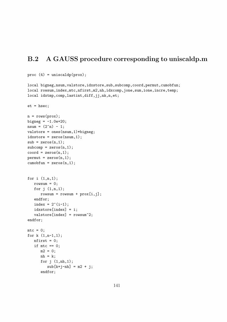
B.2 A GAUSS procedure corresponding to uniscaldp.m

proc (4) = uniscaldp(prox);

local bigneg,nsum,valstore,idxstore,sub,subcomp,coord,permut,cumobfun;local rowsum,index,mtc,nfirst,m2,nh,idxcomp,jone,sum,ione,incre,temp;local idxtmp,comp,lastint,diff,jj,nk,n,et;

et = hsec;

n = rows(prox);bigneg = -1.0e+20;nsum = (2^n) - 1;valstore = ones(nsum,1)*bigneg;idxstore = zeros(nsum,1);sub = zeros(n,1);subcomp = zeros(n,1);coord = zeros(n,1);permut = zeros(n,1);cumobfun = zeros(n,1);

for i (1,n,1);rowsum = 0;for j (1,n,1);

rowsum = rowsum + prox[i,j];endfor;index = 2^(i-1);idxstore[index] = i;valstore[index] = rowsum^2;

endfor;

mtc = 0;for k (1,n-1,1);

nfirst = 0;if mtc == 0;

m2 = 0;nh = k;for j (1,nh,1);

sub[k+j-nh] = m2 + j;endfor;

141

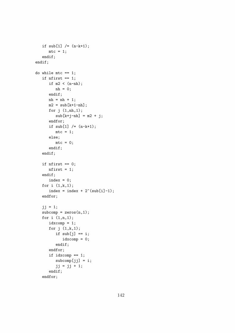
if sub[1] /= (n-k+1);mtc = 1;

endif;endif;

do while mtc == 1;if nfirst == 1;

if m2 < (n-nh);nh = 0;

endif;nh = nh + 1;m2 = sub[k+1-nh];for j (1,nh,1);

sub[k+j-nh] = m2 + j;endfor;if sub[1] /= (n-k+1);

mtc = 1;else;

mtc = 0;endif;

endif;

if nfirst == 0;nfirst = 1;

endif;index = 0;

for i (1,k,1);index = index + 2^(sub[i]-1);

endfor;

jj = 1;subcomp = zeros(n,1);for i (1,n,1);

idxcomp = 1;for j (1,k,1);

if sub[j] == i;idxcomp = 0;

endif;endfor;if idxcomp == 1;

subcomp[jj] = i;jj = jj + 1;

endif;endfor;

142

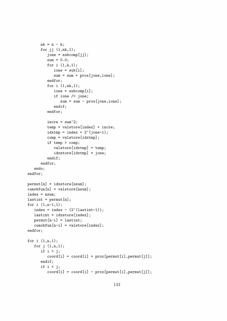
nk = n - k;for jj (1,nk,1);

jone = subcomp[jj];sum = 0.0;for i (1,k,1);

ione = sub[i];sum = sum + prox[jone,ione];

endfor;for i (1,nk,1);

ione = subcomp[i];if ione /= jone;

sum = sum - prox[jone,ione];endif;

endfor;

incre = sum^2;temp = valstore[index] + incre;idxtmp = index + 2^(jone-1);comp = valstore[idxtmp];if temp > comp;

valstore[idxtmp] = temp;idxstore[idxtmp] = jone;

endif;endfor;

endo;endfor;

permut[n] = idxstore[nsum];cumobfun[n] = valstore[nsum];index = nsum;lastint = permut[n];for i (1,n-1,1);

index = index - (2^(lastint-1));lastint = idxstore[index];permut[n-i] = lastint;cumobfun[n-i] = valstore[index];

endfor;

for i (1,n,1);for j (1,n,1);

if i > j;coord[i] = coord[i] + prox[permut[i],permut[j]];

endif;if i < j;

coord[i] = coord[i] - prox[permut[i],permut[j]];

143

endif;endfor;coord[i] = coord[i]/n;

endfor;

diff = 0;for i (1,n-1,1);

for j (i+1,n,1);diff = diff + (prox[permut[i],permut[j]] - abs(coord[i] - coord[j]))^2;

endfor;endfor;

et = hsec - et;print et;

retp(coord,permut,cumobfun,diff);

endp;

B.3 Iterative improvement Quadratic Assignment pro-

cedures

B.3.1 pairwiseqa.m

function [outperm, rawindex, allperms, index] = ...pairwiseqa(prox, targ, inperm)

% PAIRWISEQA carries out an iterative Quadratic Assignment maximization task using the% pairwise interchanges of objects in the permutation defining the row and column% order of the data matrix.% INPERM is the input beginning permutation (a permuation of the first $n$ integers).% PROX is the $n \times n$ input proximity matrix.% TARG is the $n \times n$ input target matrix.% OUTPERM is the final permutation of PROX with the cross-product index RAWINDEX% with respect to TARG.% ALLPERMS is a cell array containing INDEX entries corresponding to all the% permutations identified in the optimization from ALLPERMS1 = INPERM to% ALLPERMSINDEX = OUTPERM.

tic;begindex = sum(sum(prox(inperm,inperm).*targ));

144

outperm = inperm;nchange = 1;n = length(inperm);index = 1;allpermsindex = inperm;


nchange=0;

for k = 1:(n-1)for j = (k+1):n

intrperm = outperm;

intrperm(k) = outperm(j);intrperm(j) = outperm(k);



end

endend

end

rawindex = begindex;toc

B.3.2 rotateqa.m

function [outperm, rawindex, allperms, index] = ...rotateqa (prox, targ, inperm, kblock)

% ROTATEQA carries out a Quadratic Assignment maximization task using the% rotation of from 2 to KBLOCK% (which is less than or equal to $n-1$) consecutive objects in

145

% the permutation defining the row and column order of the data matrix.% INPERM is the input beginning permutation (a permuation of the first $n$ integers).% PROX is the $n \times n$ input proximity matrix.% TARG is the $n \times n$ input target matrix.% OUTPERM is the final permutation of PROX with the cross-product index RAWINDEX% with respect to TARG.% ALLPERMS is a cell array containing INDEX entries corresponding to all the% permutations identified in the optimization from ALLPERMS1 = INPERM to% ALLPERMSINDEX = OUTPERM.

tic;begindex = sum(sum(prox(inperm,inperm).*targ));outperm = inperm;nchange = 1;n = length(inperm);index = 1;allpermsindex = inperm;


nchange=0;


intrperm = outperm;

for j = 1:kintrperm(nlimlow+j-1) = outperm(nlimlow+k-j);

end



end

endend

end

146

rawindex = begindex;toc

B.3.3 insertqa.m

function [outperm, rawindex, allperms, index] = ...insertqa(prox, targ, inperm, kblock)

% INSERTQA carries out an iterative Quadratic Assignment maximization task using the% insertion of from 1 to KBLOCK% (which is less than or equal to $n-1$) consecutive objects in% the permutation defining the row and column order of the data matrix.% INPERM is the input beginning permutation (a permuation of the first $n$ integers).% PROX is the $n \times n$ input proximity matrix.% TARG is the $n \times n$ input target matrix.% OUTPERM is the final permutation of PROX with the cross-product index RAWINDEX% with respect to TARG.% ALLPERMS is a cell array containing INDEX entries corresponding to all the% permutations identified in the optimization from ALLPERMS1 = INPERM to% ALLPERMSINDEX = OUTPERM.

tic;begindex = sum(sum(prox(inperm,inperm).*targ));outperm = inperm;nchange = 1;n = length(inperm);index = 1;allpermsindex = inperm;


nchange=0;



intrperm = outperm;


jtwo = 0;

147

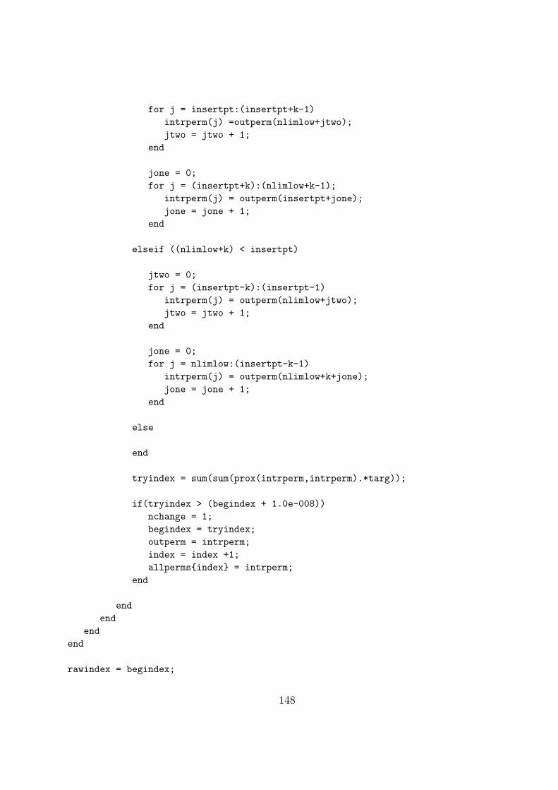
for j = insertpt:(insertpt+k-1)intrperm(j) =outperm(nlimlow+jtwo);jtwo = jtwo + 1;

end


intrperm(j) = outperm(insertpt+jone);jone = jone + 1;

end



intrperm(j) = outperm(nlimlow+jtwo);jtwo = jtwo + 1;

end


intrperm(j) = outperm(nlimlow+k+jone);jone = jone + 1;

end

else

end


if(tryindex > (begindex + 1.0e-008))nchange = 1;begindex = tryindex;outperm = intrperm;index = index +1;allpermsindex = intrperm;

end

endend

endend

rawindex = begindex;

148

toc

B.4 proxstd.m

function [stanprox, stanproxmult] = proxstd(prox,mean)

%PROXSTD produces a standardized proximity matrix (STANPROX) from the input% $n \times n$ proximity matrix (PROX) with zero main diagonal and a dissimilarity% interpretation.% STANPROX entries have unit variance (standard deviation of one) with a% mean of MEAN given as an input number;% STANPROXMULT (upper-triangular) entries have a sum of squares equal to% $n(n-1)/2$.

n = size(prox,1);aveprox = sum(sum(prox))/(n*(n-1));sumprxsq = sum(sum(prox.^2));stddev = sqrt(((1/(n*(n-1)))*sumprxsq) - ((aveprox)*(aveprox)));stanprox = zeros(n,n);stanproxmult = zeros(n,n);


if(i ~= j)

stanprox(i,j) = ((prox(i,j) - aveprox)/stddev) + mean;stanproxmult(i,j) = (n*(n-1))*(prox(i,j)/sqrt(sumprxsq));

else

stanprox(i,j) = 0.0;stanproxmult(i,j) = 0.0;

endend

end

149

B.5 proxrand.m

function [randprox] = proxrand(prox)

%PROXRAND produces a symmetric proximity matrix with a zero main diagonal having% entries that are a random permutation of those in the symmetric input proximity% matrix PROX.

n= size(prox,1);change = randperm((n*(n-1))/2);randprox = prox;

for i = 1:(n-2)for j = (i+1):n

k = i + j;

for ione = 1:(n-2)for jone = (ione+1):n

kk = ione + jone;

if(change(k) == kk)

temp = randprox(i,j);randprox(i,j) = randprox(ione,jone);randprox(j,i) = randprox(i,j);randprox(ione,jone) = temp;randprox(jone,ione) = randprox(ione,jone);

endend

end

endend

B.6 proxmon.m

150

function [monproxpermut, vaf, diff] = proxmon(proxpermut, fitted)

%PROXMON produces a monotonically transformed proximity matrix (MONPROXPERMUT)% from the order constraints obtained from each pair of entries in the input% proximity matrix PROXPERMUT (symmetric with a zero main diagonal and a dissimilarity% interpretation).% MONPROXPERMUT is close to the $n \times n$ matrix FITTED in the least-squares sense;% The variance accounted for (VAF) is how much variance in MONPROXPERMUT can be accounted for by% FITTED; DIFF is the value of the least-squares criterion.

n = size(proxpermut,1);work = zeros(n*(n-1)*n*(n-1),1);targ = proxpermut;fit = fitted;cr = 1.0;

while (cr >= 1.0e-006)

cr = 0.0;indexll = 0;


for jthree = 1:(n-1)for jfour = (jthree+1):n

if((jone ~= jthree) | (jtwo ~= jfour))

p1 = fit(jone,jtwo);p2 = fit(jthree,jfour);fit(jone,jtwo) = fit(jone,jtwo) - work(indexll+1);fit(jthree,jfour) = fit(jthree,jfour) - work(indexll+2);

if((abs(targ(jone,jtwo) - targ(jthree,jfour)) ...> 1.0e-006) & (targ(jone,jtwo) < ...targ(jthree,jfour)))

if(fit(jone,jtwo) <= fit(jthree,jfour))

work(indexll+1) = 0;work(indexll+2) = 0;

151

elseif(fit(jone,jtwo) > fit(jthree,jfour))

ave = (fit(jone,jtwo) + fit(jthree,jfour))/2.0;work(indexll+1) = ave - fit(jone,jtwo);work(indexll+2) = ave - fit(jthree,jfour);

fit(jone,jtwo) = ave;fit(jthree,jfour) = ave;

end

elseif((abs(targ(jone,jtwo) - targ(jthree,jfour)) ...> 1.0e-006) & (targ(jone,jtwo) > ...targ(jthree,jfour)))

if(fit(jone,jtwo) >= fit(jthree,jfour))

work(indexll+1) = 0;work(indexll+2) = 0;

elseif(fit(jone,jtwo) < fit(jthree,jfour))

ave = (fit(jone,jtwo) + fit(jthree,jfour))/2.0;work(indexll+1) = ave - fit(jone,jtwo);work(indexll+2) = ave - fit(jthree,jfour);fit(jone,jtwo) = ave;fit(jthree,jfour) = ave;

endend

cr = cr + abs(p1-fit(jone,jtwo)) + ...abs(p2-fit(jthree,jfour));

end

indexll = indexll + 2;

152

endend

endend

end



endend

avefit = sum(sum(fit))/(n*(n-1));


if( i ~= j)proxave(i,j) = avefit;

elseproxave(i,j) = 0;

endend

end

diff = sum(sum((fit - fitted).^2));

denom = sum(sum((fit - proxave).^2));

vaf = 1 - (diff/denom);

monproxpermut = fit;

diff = (.5)*diff;

153

B.7 matcolor.m

function matcolor(datamat,perms,numperms)

%MATCOLOR constructs a color movie of the effects of a series of% permutations on a proxmity matrix.% DATAMAT is an $n \times n$ symmetric proximity matrix;% PERMS is a cell array containing NUMPERMS permutations.

m=moviein(numperms);

for i=1:numpermspcolor(datamat(permsi,permsi));axis ij off;colormap(bone(256));colorbar;m(:,i) = getframe;

endmovie(m);

154

A Combinatorial Data Analysis Toolbox for MATLABcda.psych.uiuc.edu/cdatool/cdatoolr1.pdf · others....

Documents

Transcript of A Combinatorial Data Analysis Toolbox for MATLABcda.psych.uiuc.edu/cdatool/cdatoolr1.pdf · others....