
a bxn k Dynamics of a rational difference equation x ax A Bx k · Dynamics of a rational difference...
21
International Journal of Advances in Mathematics Volume 2018, Number 1, Pages 159-179, 2018 eISSN 2456-6098 c adv-math.com Dynamics of a rational difference equation x n+1 = ax n + α + βx n-k A + Bx n-k Abdul Khaliq * and Sk. Sarif Hassan 1 * Department of Mathematics, Riphah Institute of Computing and Applied Sciences, Riphah International University, Lahore, Pakistan. 1 Department of Mathematics, Pingla Thana Mahavidyalaya, Paschim Medinipur, 721400, West Bengal, India. E-mail: [email protected] ABSTRACT. A nonlinear rational difference equation x n+1 = ax n + α + βx n-k A + Bx n-k , n = 0, 1, ..., of higher order is considered to apprehend the dynamics viz. the invariant intervals, periodic solutions, the character of semi-cycles and global asymptotic sta- bility. Here all the parameters a, α, β and A, B and the initial conditions x k , ..., x 1 , x 0 are positive real numbers k = {1, 2, 3, ...}. It is shown that the equilibrium point is globally asymptotically stable under the condition β ≤ A, and the unique positive solu- tion is also globally asymptotically stable under the conditions β ≤ A ≤ β. Finally, we study the global stability of this equation through numerically solved examples and confirm our theoretical discussion through it. We also have considered parameters as real numbers (positive and negative) just to comprehend additional dynamics. 1 Introduction We attempt to investigate the global stability character and the periodicity of the solutions of the following rational higher order difference equation x n+1 = ax n + α + βx n-k A + Bx n-k , n = 0, 1, ..., (1.1) where the parameters a, α, β and A, B and the initial conditions x k , ..., x 1 , x 0 are positive real numbers, k = {1, 2, 3, ...} is a positive integer, and the initial conditions x -k , x -k+1 , ..., x 0 are non-negative real numbers. * Corresponding Author. Received July 18, 2017; revised September 29, 2017; accepted October 05, 2017. 2010 Mathematics Subject Classification: 39A10, 39A20, 39A99 & 39C99. Key words and phrases: Asymptotic stability, periodic solutions, equilibrium point, chaos, difference equations. This is an open access article under the CC BY license http://creativecommons.org/licenses/by/3.0/. 159
Transcript of a bxn k Dynamics of a rational difference equation x ax A Bx k · Dynamics of a rational difference...
International Journal of Advances in Mathematics
Volume 2018, Number 1, Pages 159-179, 2018
eISSN 2456-6098
c© adv-math.com
Dynamics of a rational difference equation xn+1 = axn +α + βxn−kA + Bxn−k
Abdul Khaliq∗ and Sk. Sarif Hassan1
∗Department of Mathematics, Riphah Institute of Computing and
Applied Sciences, Riphah International University, Lahore, Pakistan.1Department of Mathematics, Pingla Thana Mahavidyalaya,
Paschim Medinipur, 721400, West Bengal, India.
E-mail: [email protected]
ABSTRACT. A nonlinear rational difference equation xn+1 = axn +α + βxn−kA + Bxn−k
, n = 0, 1, ..., of higher order is considered to
apprehend the dynamics viz. the invariant intervals, periodic solutions, the character of semi-cycles and global asymptotic sta-
bility. Here all the parameters a, α, β and A, B and the initial conditions xk , ..., x1, x0 are positive real numbers k = {1, 2, 3, ...}. It
is shown that the equilibrium point is globally asymptotically stable under the condition β ≤ A, and the unique positive solu-
tion is also globally asymptotically stable under the conditions β ≤ A ≤ β. Finally, we study the global stability of this equation
through numerically solved examples and confirm our theoretical discussion through it. We also have considered parameters
as real numbers (positive and negative) just to comprehend additional dynamics.
1 Introduction
We attempt to investigate the global stability character and the periodicity of the solutions of the following rational
higher order difference equation
xn+1 = axn +α + βxn−kA + Bxn−k
, n = 0, 1, ..., (1.1)
where the parameters a, α, β and A, B and the initial conditions xk, ..., x1, x0 are positive real numbers, k =
{1, 2, 3, ...} is a positive integer, and the initial conditions x−k, x−k+1, ..., x0 are non-negative real numbers.
* Corresponding Author.
Received July 18, 2017; revised September 29, 2017; accepted October 05, 2017.
2010 Mathematics Subject Classification: 39A10, 39A20, 39A99 & 39C99.
Key words and phrases: Asymptotic stability, periodic solutions, equilibrium point, chaos, difference equations.
This is an open access article under the CC BY license http://creativecommons.org/licenses/by/3.0/.
159
Abdul Khaliq and Sk. Sarif Hassan 160
Various biological systems naturally leads to their study by means of discrete variables. Appropriate exam-
ples include ecological dynamics and medicine and etc. Some fundamental models of biological phenomena,
including harvesting of fish, a single species population model, ventilation volume and blood CO2 levels, the
production of red blood cells, a simple epidemics model, and a model of waves of disease that can be analyzed
by difference equations are shown in [1]. Newly, there has been interest in so-called dynamical diseases, which
correspond to physiological disorders for which a generally stable control system becomes unstable. One of the
first papers on this subject was that of Mackey and Glass [2]. In which they investigated a first-order difference-
delay equation that models the concentration of blood-level CO2. They also discussed models of a second class
of diseases associated with the production of red cells, white cells, and platelets in the bone marrow. The dynam-
ical characteristics of population system have been modeled, among others by differential equations in the case
of species with overlapping generations and by difference equations in the case of species with non-overlapping
generations. In process, one can develop a discrete model directly from observations and experiments. Peri-
odically, for numerical purposes, one wants to propose a finite-difference scheme to numerically solved a given
differential equation model, especially when the differential equation cannot be solved explicitly. For a given
differential equation, a difference equation approximation would be most acceptable if the solution of the differ-
ence equation is the same as the differential equation at the discrete points [3]. But unless we can explicitly solve
both equations, it is impossible to satisfy this requirements. Most of the time, it is fascinating that a differential
equation, when extracted from a difference equation, marmalade the dynamical features of the corresponding
continuous-time model such as equilibria, their local and global stability characteristics, and bifurcation behav-
iors. If alike discrete models can be derived from continuous time models, and it will preserve the considered
realities, such discrete-time models can be called ‘dynamically consistent’ with the continuous-time models.
The study of oscillatory and asymptotic stability properties of solution behavior of difference equations is
extremely advantageous in the behavior of various biological system and other applications. This is because
difference equations are relevant models for expressing situations where the variable is assumed to take only a
discrete set of values and they appear frequently in the formulation and analysis of discrete time systems, in the
study of biological systems, the study of deterministic chaos, the numerical integration of differential equations
by finite difference schemes and so on. Difference equations are good models for describing situations where
population growth is not continuous but seasonal with overlapping generations. For example, the difference
equation
xn+1 = xne
[r(1−
yn
k)
]
has been expressed to model different animal populations.
The generalized Beverton–Holt stock recruitment model has been investigated in [10,11]
xn+1 = axn +bxn−1
1 + cxn−1 + dxn.
Several other researchers have studied the behavior of the solution of difference equations, for example, in
[15] E.M. Elsayed investigated the solution of the following non-linear difference equation.
Abdul Khaliq and Sk. Sarif Hassan 161
xn+1 = axn +bx2
ncxn + dx2
n−1.
Elabbasy et al. [16] studied the boundedness, global stability, periodicity character and gave the solution of some
special cases of the difference equation.
xn+1 =αxn−l + βxn−kAxn−l + Bxn−k
.
Keratas et al. [20]gave the solution of the following difference equation
xn+1 =xn−5
1 + xn−2xn−5.
Elabbasy et al. [17] investigated the global stability, periodicity character and gave the solution of some special
cases of the difference equation
xn+1 =axn−l xn−k
bxn−p + cxn−q.
Yalcınkaya et al. [18] has studied the following difference equation
xn+1 = α +xn−m
xkn
.
Saleh et. al. [19]study the solution of difference
yn+1 = A +yn
yn−k.
Elsayed et al. [22] studied the global behavior of rational recursive sequence
xn+1 = axn−l +bxn−k + cxn−s
d + exn−t
As a matter of fact, numerous papers negotiate with the problem of solving nonlinear difference equations in
any way possible, see, for instance [7]–[15]. The long-term behavior and solutions of rational difference equations
of order greater than one has been extensively studied during the last decade. For example, various results about
periodicity, boundedness, stability, and closed form solution of the second-order rational difference equations, see
[5–9, 21–29]. Other related work on rational difference equations see in refs. [30–44]
Here, we recall some basic definitions and some theorems that we need in the sequel.
Let I be some interval of real numbers and let F : Ik+1 → I, be a continuously differentiable function. Then
for every set of initial conditions x−k, x−k+1, ...,x0 ∈ I, the difference equation
xn+1 = F(xn, xn−1, ..., xn−k), n = 0, 1, ..., (1.2)
has a unique solution {xn}∞n=−k.
(Equilibrium Point) A point x ∈ I is called an equilibrium point of Eq.(1.2) if
x = F(x, x, ..., x).
That is, xn = x for n ≥ 0, is a solution of Eq.(1.2), or equivalently, x is a fixed point of F.
Abdul Khaliq and Sk. Sarif Hassan 162
(Periodicity) A Sequence {xn}∞n=−k is said to be periodic with period p if xn+p = xn for all n ≥ −k.
(Fibonacci Sequence). The sequence {Fm}∞m=1 = {1, 2, 3, 5, 8, 13, ....}i.e. Fm = Fm−1 + Fm−2 ≥ 0, F−2 = 0, F−1 =
1 is called Fibonacci Sequence.
(Stability)
(i) The equilibrium point x of Eq.(1.2) is locally stable if for every ε > 0, there exists δ > 0 such that for all
x−k, x−k+1, ..., x−1,x0 ∈ I with
|x−k − x|+ |x−k+1 − x|+ ... + |x0 − x| < δ,
we have
|xn − x| < ε for all n ≥ −k.
(ii) The equilibrium point x of Eq.(1.2) is locally asymptotically stable if x is locally stable solution of Eq.(1.2) and
there exists γ > 0, such that for all x−k, x−k+1, ..., x−1, x0 ∈ I with
|x−k − x|+ |x−k+1 − x|+ ... + |x0 − x| < γ,
we have
limn→∞
xn = x.
(iii) The equilibrium point x of Eq.(1.2) is global attractor if for all x−k, x−k+1, ..., x−1, x0 ∈ I, we have
limn→∞
xn = x.
(iv) The equilibrium point x of Eq.(1.2) is globally asymptotically stable if x is locally stable, and x is also a global
attractor of Eq.(1.2).
(v) The equilibrium point x of Eq.(1.2) is unstable if x is not locally stable.
(vi) The linearized equation of Eq.(1.2) about the equilibrium x is the linear difference equation
yn+1 =k
∑i=0
∂F(x, x, ..., x)∂xn−i
yn−i. (1.3)
Theorem A [27] Assume that p, q ∈ R and k ∈ {0, 1, 2, ...}. Then
|p|+ |q| < 1, (1.4)
is a sufficient condition for the asymptotic stability of the difference equation
xn+1 + pxn + qxn−k = 0, n = 0, 1, ... .
The following theorem will be useful for the proof of our results in this paper.
Theorem B [28]: Let [l, m] be an interval of real numbers and assume that f : [l, m]2 → [l, m],is a continuous
function and consider the following equation
xn+1 = f (xn, xn−1), n = 0, 1, ..., (1.5)
satisfying the following conditions :
Abdul Khaliq and Sk. Sarif Hassan 163
(a) f (x, y) is non-decreasing in x ∈ [l, m] for each fixed y ∈ [α, β].and g(x, y) is non-increasing in y ∈ [l, m] for
each fixed x ∈ [l, m]
(b) If (m, M) ∈ [l, m]× [l, m] is a solution of the system
M = g(M, m) and m = g(m, M),
then m = M,
then Eq. (5) has a unique equilibrium x ∈ [l, m] and every solution of Eq.(5) converges to x.
2 Equilibrium points of Eq.(1.1)
In this section we shall study the equilibrium points of Eq.(1.1) and their computational existence. The equilibrium
points of Eq.(1.1) are the solutions of the equation
x = ax +α + βxA + Bx
or,
B(1− a)x2 + (A− Aa− β)x− α = 0
The solution of the Eq.(1) are√
(−aA+A−β)2+4α(B−aB)−aA+A−β
2(aB−B) and√
(−aA+A−β)2+4α(B−aB)+aA−A+β
2(B−aB) . Then the
only positive equilibrium point of Eq.(1)for all the positive parameters a, α, β and A, B is given by
x =(β− A + Aa) +
√(β− A + Aa)2 + 4αB(1− a)2B(1− a)
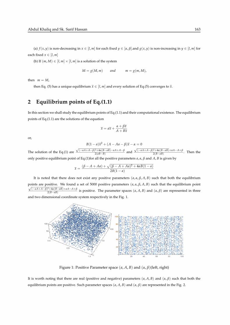
It is noted that there does not exist any positive parameters (a, α, β, A, B) such that both the equilibrium
points are positive. We found a set of 5000 positive parameters (a, α, β, A, B) such that the equilibrium point√(−aA+A−β)2+4α(B−aB)+aA−A+β
2(B−aB) is positive. The parameter spaces (a, A, B) and (α, β) are represented in three
and two dimensional coordinate system respectively in the Fig. 1.
Figure 1: Positive Parameter space (a, A, B) and (α, β)(left, right)
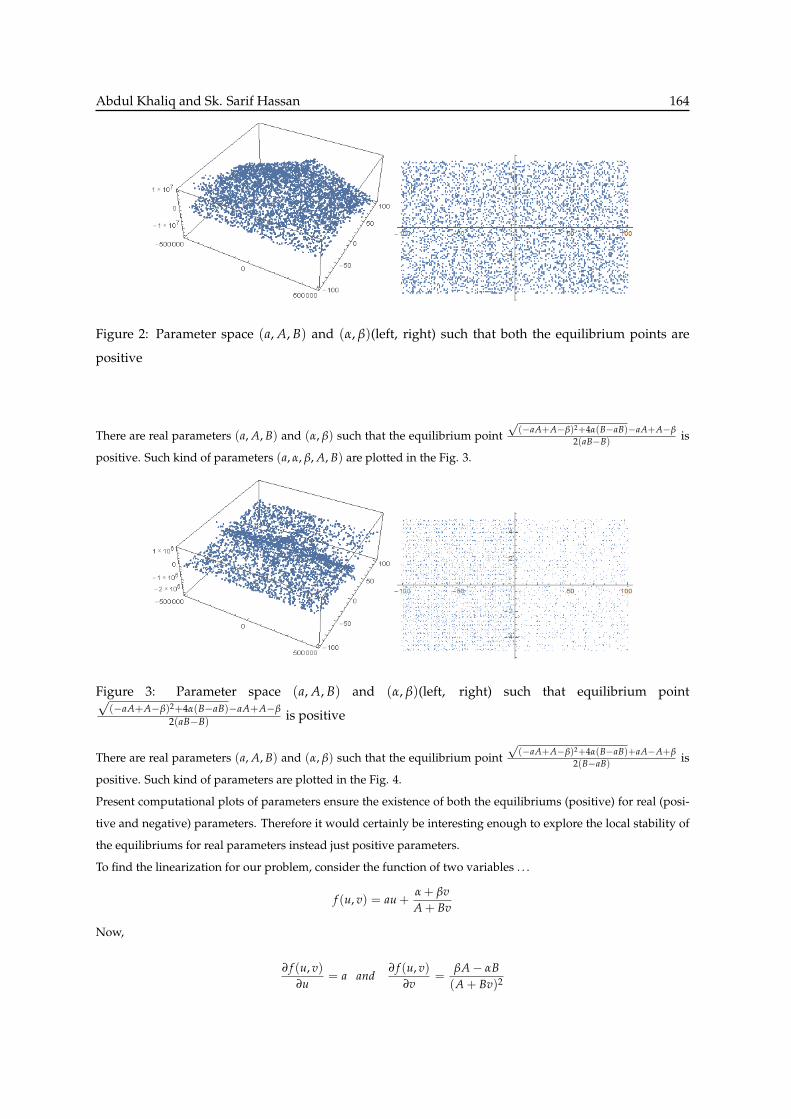
It is worth noting that there are real (positive and negative) parameters (a, A, B) and (α, β) such that both the
equilibrium points are positive. Such parameter spaces (a, A, B) and (α, β) are represented in the Fig. 2.
Abdul Khaliq and Sk. Sarif Hassan 164
Figure 2: Parameter space (a, A, B) and (α, β)(left, right) such that both the equilibrium points are
positive
There are real parameters (a, A, B) and (α, β) such that the equilibrium point√
(−aA+A−β)2+4α(B−aB)−aA+A−β
2(aB−B) is
positive. Such kind of parameters (a, α, β, A, B) are plotted in the Fig. 3.
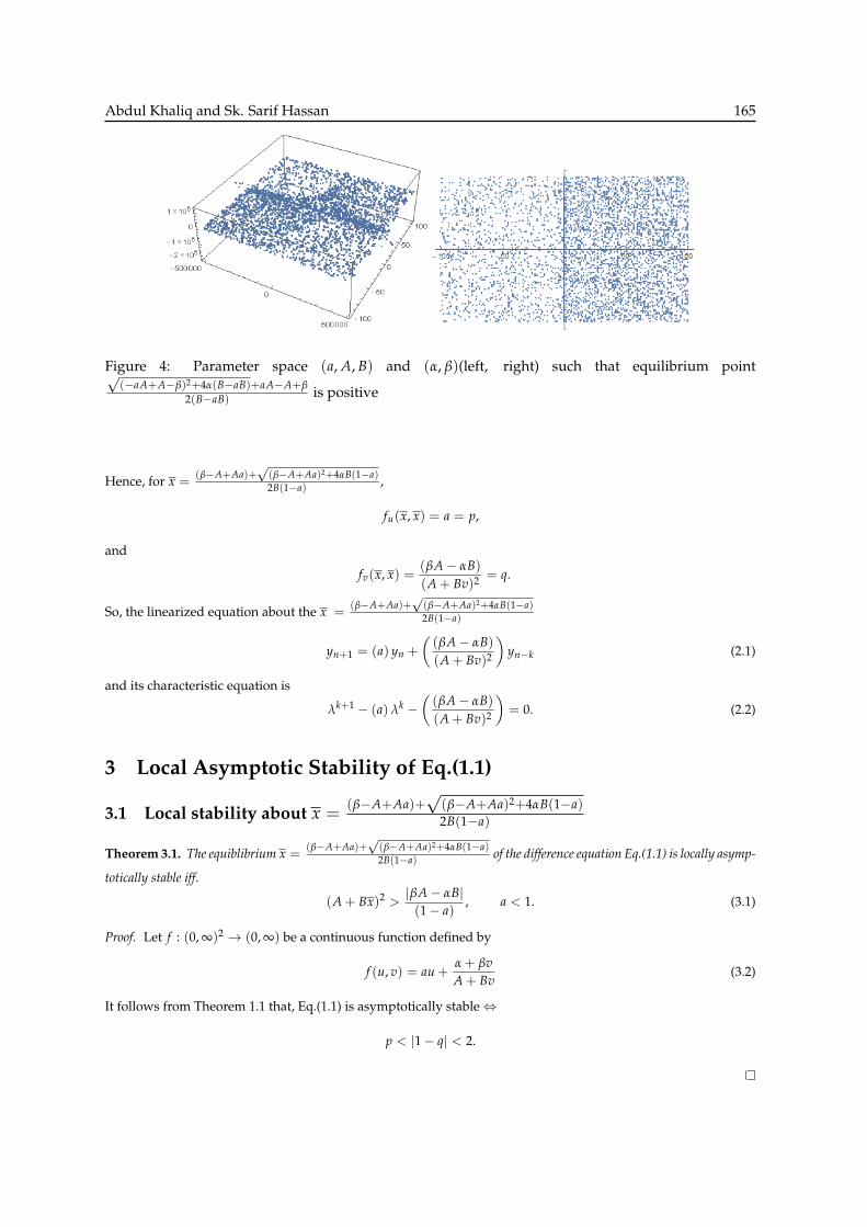
Figure 3: Parameter space (a, A, B) and (α, β)(left, right) such that equilibrium point√(−aA+A−β)2+4α(B−aB)−aA+A−β
2(aB−B) is positive
There are real parameters (a, A, B) and (α, β) such that the equilibrium point√
(−aA+A−β)2+4α(B−aB)+aA−A+β
2(B−aB) is
positive. Such kind of parameters are plotted in the Fig. 4.
Present computational plots of parameters ensure the existence of both the equilibriums (positive) for real (posi-
tive and negative) parameters. Therefore it would certainly be interesting enough to explore the local stability of
the equilibriums for real parameters instead just positive parameters.
To find the linearization for our problem, consider the function of two variables . . .
f (u, v) = au +α + βvA + Bv
Now,
∂ f (u, v)∂u
= a and∂ f (u, v)
∂v=
βA− αB(A + Bv)2
Abdul Khaliq and Sk. Sarif Hassan 165
Figure 4: Parameter space (a, A, B) and (α, β)(left, right) such that equilibrium point√(−aA+A−β)2+4α(B−aB)+aA−A+β
2(B−aB) is positive
Hence, for x =(β−A+Aa)+
√(β−A+Aa)2+4αB(1−a)2B(1−a) ,
fu(x, x) = a = p,
and
fv(x, x) =(βA− αB)(A + Bv)2 = q.
So, the linearized equation about the x =(β−A+Aa)+
√(β−A+Aa)2+4αB(1−a)2B(1−a)
yn+1 = (a) yn +
((βA− αB)(A + Bv)2
)yn−k (2.1)
and its characteristic equation is
λk+1 − (a) λk −((βA− αB)(A + Bv)2
)= 0. (2.2)
3 Local Asymptotic Stability of Eq.(1.1)
3.1 Local stability about x =(β−A+Aa)+
√(β−A+Aa)2+4αB(1−a)2B(1−a)
Theorem 3.1. The equiblibrium x =(β−A+Aa)+
√(β−A+Aa)2+4αB(1−a)2B(1−a) of the difference equation Eq.(1.1) is locally asymp-
totically stable iff.
(A + Bx)2 >|βA− αB|(1− a)
, a < 1. (3.1)
Proof. Let f : (0, ∞)2 → (0, ∞) be a continuous function defined by
f (u, v) = au +α + βvA + Bv
(3.2)
It follows from Theorem 1.1 that, Eq.(1.1) is asymptotically stable⇔
p < |1− q| < 2.
Abdul Khaliq and Sk. Sarif Hassan 166
Thus,
a +∣∣∣∣ (βA− αB)(A + Bv)2
∣∣∣∣ < 1,
also ∣∣∣∣ (βA− αB)(A + Bv)2
∣∣∣∣ < (1− a), a < 1,
|βA− αB| < (A + Bv)2(1− a), a < 1,
or|βA− αB|(1− a)
< (A + Bv)2, a < 1.
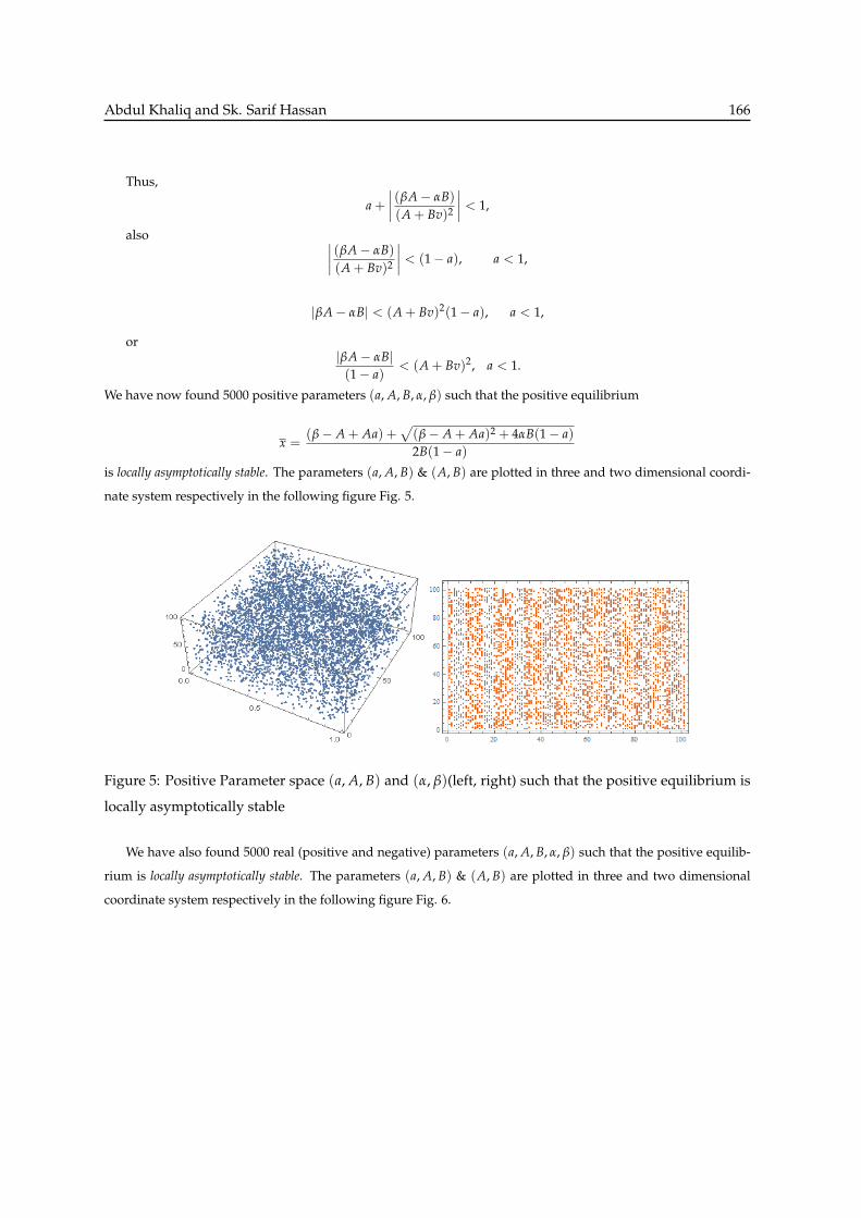
We have now found 5000 positive parameters (a, A, B, α, β) such that the positive equilibrium
x =(β− A + Aa) +
√(β− A + Aa)2 + 4αB(1− a)2B(1− a)
is locally asymptotically stable. The parameters (a, A, B) & (A, B) are plotted in three and two dimensional coordi-
nate system respectively in the following figure Fig. 5.
Figure 5: Positive Parameter space (a, A, B) and (α, β)(left, right) such that the positive equilibrium is
locally asymptotically stable
We have also found 5000 real (positive and negative) parameters (a, A, B, α, β) such that the positive equilib-
rium is locally asymptotically stable. The parameters (a, A, B) & (A, B) are plotted in three and two dimensional
coordinate system respectively in the following figure Fig. 6.
Abdul Khaliq and Sk. Sarif Hassan 167
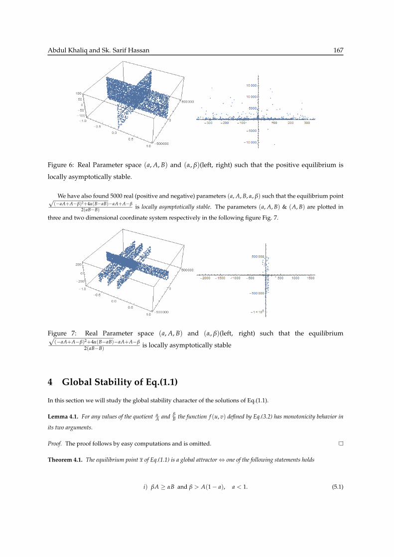
Figure 6: Real Parameter space (a, A, B) and (α, β)(left, right) such that the positive equilibrium is
locally asymptotically stable.
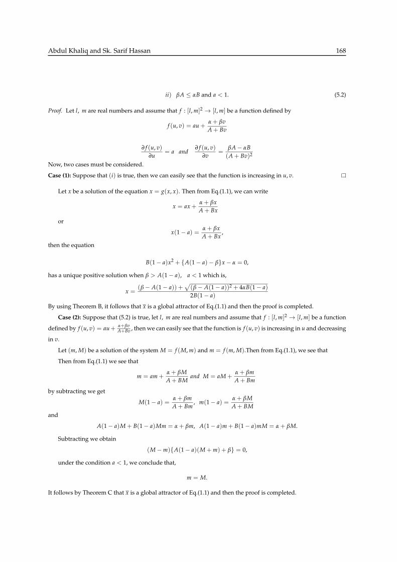
We have also found 5000 real (positive and negative) parameters (a, A, B, α, β) such that the equilibrium point√(−aA+A−β)2+4α(B−aB)−aA+A−β
2(aB−B) is locally asymptotically stable. The parameters (a, A, B) & (A, B) are plotted in
three and two dimensional coordinate system respectively in the following figure Fig. 7.
Figure 7: Real Parameter space (a, A, B) and (α, β)(left, right) such that the equilibrium√(−aA+A−β)2+4α(B−aB)−aA+A−β
2(aB−B) is locally asymptotically stable
4 Global Stability of Eq.(1.1)
In this section we will study the global stability character of the solutions of Eq.(1.1).
Lemma 4.1. For any values of the quotient αA and β
B the function f (u, v) defined by Eq.(3.2) has monotonicity behavior in
its two arguments.
Proof. The proof follows by easy computations and is omitted.
Theorem 4.1. The equilibrium point x of Eq.(1.1) is a global attractor⇔ one of the following statements holds
i) βA ≥ αB and β > A(1− a), a < 1. (5.1)
Abdul Khaliq and Sk. Sarif Hassan 168
ii) βA ≤ αB and a < 1. (5.2)
Proof. Let l, m are real numbers and assume that f : [l, m]2 → [l, m] be a function defined by
f (u, v) = au +α + βvA + Bv
∂ f (u, v)∂u
= a and∂ f (u, v)
∂v=
βA− αB(A + Bv)2
Now, two cases must be considered.
Case (1): Suppose that (i) is true, then we can easily see that the function is increasing in u, v.
Let x be a solution of the equation x = g(x, x). Then from Eq.(1.1), we can write
x = ax +α + βxA + Bx
or
x(1− a) =α + βxA + Bx
,
then the equation
B(1− a)x2 + {A(1− a)− β}x− α = 0,
has a unique positive solution when β > A(1− a), a < 1 which is,
x =(β− A(1− a)) +
√(β− A(1− a))2 + 4αB(1− a)2B(1− a)
By using Theorem B, it follows that x is a global attractor of Eq.(1.1) and then the proof is completed.
Case (2): Suppose that (5.2) is true, let l, m are real numbers and assume that f : [l, m]2 → [l, m] be a function
defined by f (u, v) = au+α+βvA+Bv , then we can easily see that the function is f (u, v) is increasing in u and decreasing
in v.
Let (m, M) be a solution of the system M = f (M, m) and m = f (m, M).Then from Eq.(1.1), we see that
Then from Eq.(1.1) we see that
m = am +α + βMA + BM
and M = aM +α + βmA + Bm
by subtracting we get
M(1− a) =α + βmA + Bm
, m(1− a) =α + βMA + BM
and
A(1− a)M + B(1− a)Mm = α + βm, A(1− a)m + B(1− a)mM = α + βM.
Subtracting we obtain
(M−m){A(1− a)(M + m) + β} = 0,
under the condition a < 1, we conclude that,
m = M.
It follows by Theorem C that x is a global attractor of Eq.(1.1) and then the proof is completed.
Abdul Khaliq and Sk. Sarif Hassan 169
5 Boundedness of Solution of Eq.(1.1)
In this section we will study the boundedness of solutions of Eq.(1.1).
Theorem 5.1. Every solution of Eq.(1.1) is boumded and persist if a < 1.
Proof. Let {xn}∞n=−k be a solution of Eq. (1.1). It follows from Eq. (1.1) that
xn+1 = axn +α + βxn−kA + Bxn−k
= axn +α
A + Bxn−k+
βxn−kA + Bxn−k
Then
xn+1 ≤ axn +α
A+
βxn−kBxn−k
= axn +α
A+
β
Bf or all n ≥ 1.
By using comparison, the right hand side can be written as follows
yn+1 = ayn +α
A+
β
B.
So, we can write
yn = any0 + constant,
and this equation is locally asymptotically stable because a < 1, and converges to the equillibrium point y =
αB+βAAB(1−a)
Therefore
limn→∞
sup xn ≤αB + βA
AB(1− a)
Hence the solution is bounded.
Theorem 5.2. Every solution of Eq.(1.1) is bounded is unbounded if a > 1.
Proof. Let {xn}∞n=−1be a solution of Eq.(1.1). Then from Eq.(1.1) we see that
xn+1 = axn +α + βxn−kA + Bxn−k
> axn f or all n ≥ 1.
the right hand side can be written as follows
yn+1 = ayn ⇒ yn = any0,
and this equation is unstable because a > 1, and limn→∞ yn = ∞. Then by using ratio test {xn}∞n=−1is unbounded
from above.
Abdul Khaliq and Sk. Sarif Hassan 170
6 Existence of Periodic Solution
In this section, we are looking for the positive prime period two solution of Eq.(1.1). Let us assume the two cycle
period of Eq.(1.1) will be in the form
...p, q, p, q...
Case (1): if k is odd then,
xn+1 = xn−k (4.1)
we get,
p = aq +α + βpA + Bp
q = ap +α + βqA + Bq
This transform to
Ap + Bp2 = aAq + aBpq + α + βp and
Aq + Bq2 = aAp + aBpq + α + βq.
by subtracting (4.5) from (4.4) we get,
A(p− q) + B(p2 − q2) = −aA(p− q) + β(p− q)
Then since p 6= q, it follows that
(p + q) =β− aA− A
B(4.4)
again by adding (4.5) from (4.4) we get,
A(p + q) + B(p2 + q2) = aA(p + q) + 2aBpq + 2α + β(p + q),
B(p2 + q2) = (aA− A + β)(p + q) + 2aBpq + 2α
By using (4.4), (4.5) and the relation
p2 + q2 = (p + q)2 − 2pq, p, q ∈ R,
we get
B((p + q)2 − 2pq) = (aA− A + β)(p + q) + 2aBpq + 2α
2(1 + a)Bpq = −2aA(p + q)− 2α
So,
pq =−(β− aA− A)aA− αB
(1 + a)B2 . (4.5)
Now, it is obvious from Eq.(4.4) and Eq.(4.5) that, p and q are two distinct real roots of the quadratic equation
t2 −(
β− aA− AB
)t−(
αB + (β− aA− A)aA(1 + a)B2
)= 0,
or,
Bt2 − (β− aA− A)t−(
αB + (β− aA− A)aA(1 + a)B
)= 0,
Abdul Khaliq and Sk. Sarif Hassan 171
Thus,
[β− aA− A]2 +4 [αB + (β− aA− A)aA]
(1 + a)> 0, (4.6)
or
[β− aA− A]2 (1 + a) + 4 [αB + (β− aA− A)aA] > 0.
Now suppose,
p =β− aA− A + δ
2Band
q =β− aA− A− δ
2B
where δ =
√[β− aA− A]2 +
4[αB+(β−aA−A)aA](1+a)
from (4.6) we get that δ2 > 0, therefore p and q are distinct real numbers, set
x−1 = p and x0 = q.
It follows from Eq.(1.1) that
x1 = aq +α + βpA + Bp
= a(
β− aA− A− δ
2B
)+
α + β(
β−aA−A−δ2B
)A + B
(β−aA−A−δ
2B
)dividing numerator and denominator by 2(A + aB) we get
x1 = a(
β− aA− A + δ
2B
)+
2Bα + β(β− aA− A + δ)
2BA + B(β− aA− A + δ)
multiply denominator and numerator of right hand side by 2BA + B(β− aA− A− δ) and by computation we get
x1 = p
Similarly
x2 = q
Then by induction we get
x2n = q and x2n+1 = p for all n ≥ −1.
Thus Eq.(1.1) has prime period two solution.
Case (2): if k is even then
p = aq +α + βqA + Bq
q = ap +α + βpA + Bp
This transforms to
Ap + Bpq = aAq + aBq2 + α + βq
Aq + Bpq = aAp + aBp2 + α + βp
Abdul Khaliq and Sk. Sarif Hassan 172
by subtracting (4.8) from (4.7) we get,
A(p− q) = −aA(p− q)− aB(p2 − q2)− β(p− q)
Then since p 6= q, it follows that
(p + q) = −(
β + aA + AaB
)(4.9)
again by adding (4.7) from (4.8) we get,
A(p + q) + 2Bpq = aA(p + q) + aB(p2 + q2) + 2α + β(p + q),
aB(p2 + q2) = (A− aA− β)(p + q) + 2aBpq− 2α.
by using (4.7), (4.8) and the relation
p2 + q2 = (p + q)2 − 2pq, p, q ∈ R,
we get
aB((p + q)2 − 2pq) = (A− aA− β)(p + q) + 2aBpq− 2α
4aBpq = 2α− 2A.
So,
pq =α− A2aB
. (4.10)
Now, it is obvious from Eq.(4.4) and Eq.(4.5) that, p and q are two distint real roots of the quadratic equation
t2 +
(β + aA + A
aB
)t−(
α− A2aB
)= 0,
or,
2aBt2 + 2(β + aA + A)t− (α− A) = 0,
Thus,
4(β + aA + A)2 + 8aB(α− A) > 0. (4.11)
Now suppose,
p =−2(β + aA + A) + δ
4aBand
q =−2(β + aA + A)− δ
4aBwhere δ =
√4(β + aA + A)2 + 8aB(α− A)
from (4.6) we get that δ2 > 0, therefore p and q are distinct real numbers, set
x−1 = p and x0 = q.
It follows from Eq.(1.1) that
x1 = aq +α + βqA + Bq
= a(−2(β + aA + A)− δ
4aB
)+
α + β(−2(β+aA+A)−δ
4aB
)A + B
(−2(β+aA+A)−δ
4aB
)
Abdul Khaliq and Sk. Sarif Hassan 173
so,
x1 = −a((β + aA + A)− δ
2aB
)+
4aBα + β(−2(β + aA + A)− δ)
4aBA + B(−2(β + aA + A)− δ)
multiply denominator and numerator of right hand side by 4aBA + B(−2(β + aA + A) + δ) and by computation
we get
x1 = p
Similarly
x2 = q
Then by induction we get
x2n = q and x2n+1 = p for all n ≥ −1.
Thus Eq.(1.1) has prime period two solution.
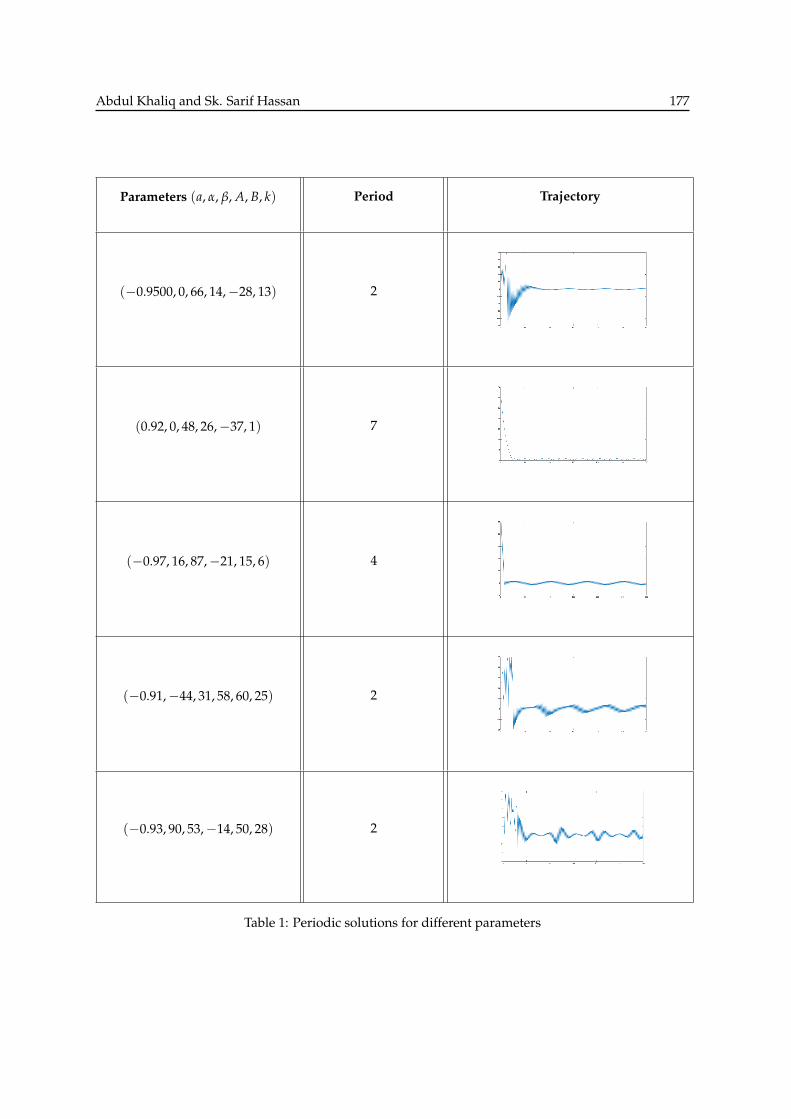
Here we shall explore real parameters (a, α, β, A, B) and k such that the solutions of the rational difference equation
Eq.(1.1) are periodic, which is listed in the Table 1.
It is noted that, in all the cases, the periodic solution exist if the parameter |a| < 1.
7 Existence of Chaotic Solution
Here computationally we wish to explore solution of the rational difference equation of chaotic nature. We assume
here the parameters are real numbers. This assumption is based on the impression that there does not exist such
dynamics for any strictly positive real parameters of the system. Here we gathered a set of examples as stated in
the following Table 2.
In all the above set of examples of chaotic cases, without loss of generality, the parameters A, B, α, β are taken
from the interval [−100, 100] and a is taken to be absolutely less than 1. Also k is taken from the interval [1, 50]. In
every case, ten different initial values are taken and ran the trajectory for the specific set parameters.
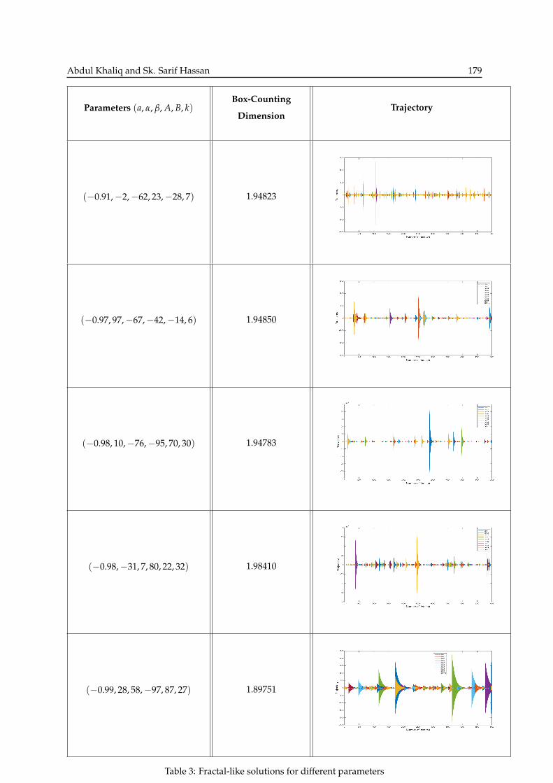
8 Existence of Fractal-like Solution
Computationally we explore solutions of the rational difference equation of self-similar (fractal-like) nature. We
assume here as usual the parameters are real numbers. Here we gathered a set of examples as stated in the
following Table 2.
In all the above set of examples of fractal-like(self-similar), without loss of generality, the parameters A, B, α, β
are taken from the interval [−100, 100] and a is taken to be absolutely less than 1. Also k is taken from the interval
[1, 50]. In every case, ten different initial values are taken and ran the trajectory for the specific set parameters.
Abdul Khaliq and Sk. Sarif Hassan 174
References
[1] A.M. Ahmed, and A.M. Youssef, A solution form of a class of higher-order rational difference equations, J.
Egyp. Math. Soc., 21 (2013), 248–253.
[2] M. Aloqeili, Global stability of a rational symmetric difference equation, Appl. Math. Comp., 215 (2009) 950-
953.
[3] M. Aprahamian, D. Souroujon, and S. Tersian, Decreasing and fast solutions for a second-order difference
equation related to Fisher-Kolmogorov’s equation, J. Math. Anal. Appl. 363 (2010), 97-110.
[4] H. Chen and H. Wang, Global attractivity of the difference equation xn+1 =xn + αxn−1
β + xn, Appl. Math. Comp.,
181 (2006) 1431–1438.
[5] C. Cinar, On the positive solutions of the difference equation xn+1 =axn−1
1 + bxnxn−1, Appl. Math. Comp., 156
(2004) 587-590.
[6] S. E. Das and M.Bayram, On a System of Rational Difference Equations, World Applied Sciences Journal
10(11) (2010), 1306-1312.
[7] Q. Din, and E. M. Elsayed, Stability analysis of a discrete ecological model, Computational Ecology and
Software 4 (2) (2014), 89–103.
[8] E. M. Elabbasy, H. El-Metwally and E. M. Elsayed, On the difference equations xn+1 =αxn−k
β + γ ∏ki=0 xn−i
, J.
Conc. Appl. Math., 5(2) (2007), 101-113.
[9] E. M. Elabbasy, H. El-Metwally and E. M. Elsayed, Qualitative behavior of higher order difference equation,
Soochow Journal of Mathematics, 33 (4) (2007), 861-873.
[10] E. M. Elabbasy, H. El-Metwally and E. M. Elsayed, On the Difference Equation xn+1 = a0xn+a1xn−1+...+ak xn−kb0xn+b1xn−1+...+bk xn−k
,
Mathematica Bohemica, 133 (2) (2008), 133-147.
[11] H. El-Metwally, Global behavior of an economic model, Chaos, Solitons and Fractals, 33 (2007), 994–1005.
[12] H. El-Metwally and M. M. El-Afifi, On the behavior of some extension forms of some population models,
Chaos, Solitons and Fractals, 36 (2008), 104–114.
[13] H. El-Metwally and E. M. Elsayed, Form of solutions and periodicity for systems of difference equations,
Journal of Computational Analysis and Applications, 15(5) (2013), 852-857.
[14] E. M. Elsayed, Behavior and expression of the solutions of some rational difference equations, Journal of
Computational Analysis and Applications, 15 (1) (2013), 73-81.
[15] E. M. Elsayed, Solution for systems of difference equations of rational form of order two, Computational and
Applied Mathematics, 33 (3) (2014), 751-765.
[16] E. M. Elsayed and H. El-Metwally, Global Behavior and Periodicity of Some Difference Equations, Journal of
Computational Analysis and Applications, 19 (2) (2015), 298-309.
[17] E. M. Elsayed, Dynamics of a Recursive Sequence of Higher Order, Communications on Applied Nonlinear
Analysis, 16 (2) (2009), 37–50.
Abdul Khaliq and Sk. Sarif Hassan 175
[18] E. M. Elsayed, Qualitative behavior of difference equation of order three, Acta Scientiarum Mathematicarum
(Szeged), 75 (1-2), 113–129.
[19] E. M. Elsayed, Qualitative behavior of difference equation of order two, Mathematical and Computer Mod-
elling, 50 (2009), 1130–1141.
[20] R. Karatas, C. Cinar and D. Simsek, On positive solutions of the difference equation xn+1 =xn−5
1 + xn−2xn−5,
Int. J. Contemp. Math. Sci., Vol. 1, 2006, no. 10, 495-500.
[21] V. L. Kocic and G. Ladas, Global Behavior of Nonlinear Difference Equations of Higher Order with Applica-
tions, Kluwer Academic Publishers, Dordrecht, 1993.
[22] M. R. S. Kulenovic and G. Ladas, Dynamics of Second Order Rational Difference Equations with Open Prob-
lems and Conjectures, Chapman & Hall / CRC Press, 2001.
[23] A. S. Kurbanli, On the Behavior of Solutions of the System of Rational Difference Equations, World Applied
Sciences Journal, 10 (11) (2010), 1344-1350.
[24] R. Memarbashi, Sufficient conditions for the exponential stability of nonautonomous difference equations,
Appl. Math. Letter 21 (2008) 232–235.
[25] A. Neyrameh, H. Neyrameh, M. Ebrahimi and A. Roozi, Analytic solution diffusivity equation in rational
form, World Applied Sciences Journal, 10 (7) (2010), 764-768.
[26] M. Saleh and M. Aloqeili, On the difference equation yn+1 = A +yn
yn−kwith A < 0, Appl. Math. Comp.,
176(1) (2006), 359–363.
[27] M. Saleh and M. Aloqeili, On the difference equation xn+1 = A +xn
xn−k, Appl. Math. Comp., 171 (2005),
862-869.
[28] T. Sun and H. Xi, On convergence of the solutions of the difference equation xn+1 = 1+xn−1
xn, J. Math. Anal.
Appl. 325 (2007) 1491–1494.
[29] C. Wang, S. Wang, L. LI, Q. Shi, Asymptotic behavior of equilibrium point for a class of nonlinear difference
equation, Advances in Difference Equations, Volume 2009, Article ID 214309. 8pages.
[30] C. Wang, S. Wang, Z. Wang, H. Gong, R. Wang, Asymptotic stability for a class of nonlinear difference
equation, Discrete Dynamics in Natural and Society, Volume 2010, Article ID 791610, 10pages.
[31] I. Yalcınkaya, On the global asymptotic stability of a second-order system of difference equations, Discrete
Dynamics in Nature and Society, Vol. 2008, Article ID 860152, 12 pages, doi: 10.1155/2008/ 860152.
[32] I. Yalcınkaya, On the difference equation xn+1 = α + xn−mxk
n, Discrete Dynamics in Nature and Society, Vol.
2008, Article ID 805460, 8 pages, doi: 10.1155/2008/ 805460.
[33] E. M. E. Zayed and M. A. El-Moneam, On the rational recursive sequence xn+1 =α+βxn+γxn−1A+Bxn+Cxn−1
, Communi-
cations on Applied Nonlinear Analysis, 12 (4) (2005), 15–28.
[34] E. M. E. Zayed and M. A. El-Moneam, On the rational recursive sequence xn+1 =αxn+βxn−1+γxn−2+δxn−3
Axn+Bxn−1+Cxn−2+Dxn−3;
Comm. Appl. Nonlinear Analysis, 12 (2005), 15-28.
Abdul Khaliq and Sk. Sarif Hassan 176
[35] B. G. Zhang, C. J. Tian and P. J. Wong, Global attractivity of difference equations with variable delay, Dyn.
Contin. Discrete Impuls. Syst., 6(3) (1999), 307–317.
[36] Wan-Tong Li, Hong-Rui Sun, Dynamics of a rational difference equation, Applied Mathematics and Compu-
tation Volume 163, Issue 2, 15 April 2005, Pages 577-591.
[37] Lin-Xia Hu, Wan-Tong Li, Hong-Wu Xu, Global asymptotical stability of a second order rational difference
equation, Computers & Mathematics with Applications archive Volume 54 Issue 9-10, November, 2007 Pages
1260-1266.
[38] You-Hui Su, Wan Tong Li, Stevo Stevic, Dynamics of a higher order nonlinear rational difference equation,
Journal of Difference Equations and Applications, Vol. 11, Iss. 2, 2005.
[39] Li X. Global behavior for a fourth-order rational difference equation. Journal of Mathematical Analysis and
Applications. 2005 Dec 15;312(2):555-63.
[40] Berenhaut KS, Stevi S. The global attractivity of a higher order rational difference equation. Journal of Math-
ematical Analysis and Applications. 2007 Feb 15;326(2):940-4.
[41] Elsayed EM. Solution and attractivity for a rational recursive sequence. Discrete Dynamics in Nature and
Society. 2011 Jun 8;2011.
[42] Stevi S. Nontrivial solutions of a higher-order rational difference equation. Mathematical Notes. 2008 Nov
1;84.
[43] Saleh M, Abu-Baha S. Dynamics of a higher order rational difference equation. Applied Mathematics and
Computation. 2006 Oct 1;181(1):84-102.
[44] Aloqeili M. Dynamics of a kth order rational difference equation. Applied Mathematics and Computation.
2006 Oct 15;181(2):1328-35.
Abdul Khaliq and Sk. Sarif Hassan 177
Parameters (a, α, β, A, B, k) Period Trajectory
(−0.9500, 0, 66, 14,−28, 13) 2
(0.92, 0, 48, 26,−37, 1) 7
(−0.97, 16, 87,−21, 15, 6) 4
(−0.91,−44, 31, 58, 60, 25) 2
(−0.93, 90, 53,−14, 50, 28) 2
Table 1: Periodic solutions for different parameters
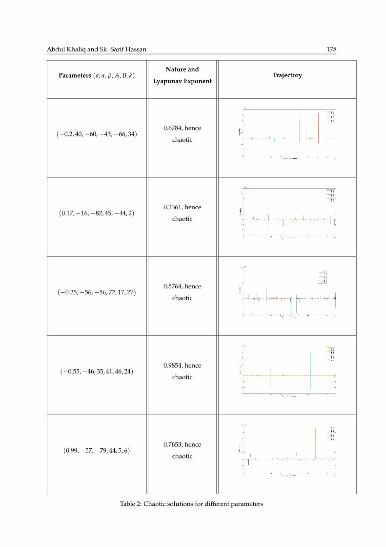
Abdul Khaliq and Sk. Sarif Hassan 178
Parameters (a, α, β, A, B, k)Nature and
Lyapunav ExponentTrajectory
(−0.2, 40,−60,−43,−66, 34)0.6784, hence
chaotic
(0.17,−16,−82, 45,−44, 2)0.2361, hence
chaotic
(−0.25,−56,−56, 72, 17, 27)0.5764, hence
chaotic
(−0.55,−46, 35, 41, 46, 24)0.9854, hence
chaotic
(0.99,−57,−79, 44, 5, 6)0.7653, hence
chaotic
Table 2: Chaotic solutions for different parameters
Abdul Khaliq and Sk. Sarif Hassan 179
Parameters (a, α, β, A, B, k)Box-Counting
DimensionTrajectory
(−0.91,−2,−62, 23,−28, 7) 1.94823
(−0.97, 97,−67,−42,−14, 6) 1.94850
(−0.98, 10,−76,−95, 70, 30) 1.94783
(−0.98,−31, 7, 80, 22, 32) 1.98410
(−0.99, 28, 58,−97, 87, 27) 1.89751
Table 3: Fractal-like solutions for different parameters


![Point clustering with a convex, corrected K-means · k: X a= k+ E a with E[X a] = k and E a ˘ ind sub-N(0; a) Key quantities to keep in mind: cluster separation G( ) := min k6=lj](https://static.fdocument.org/doc/165x107/5f057b917e708231d4132efa/point-clustering-with-a-convex-corrected-k-k-x-a-k-e-a-with-ex-a-k-and.jpg)


![Finite Element Clifford Algebra: A New Toolkit for ...ccom.ucsd.edu/~agillette/research/pd11talk.pdf · [0;T] k+2 [0;T] k+1 d 6 (r k d 6 (r k k 1 d 6 (r k 2 Finite Element Clifford](https://static.fdocument.org/doc/165x107/5f58bc148149db2e4503093f/finite-element-clifford-algebra-a-new-toolkit-for-ccomucsdeduagilletteresearch.jpg)