
A Brief and Friendly(?) Introduction to hierarchical...
202
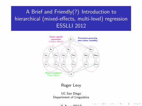
A Brief and Friendly(?) Introduction to hierarchical (mixed-effects, multi-level) regression ESSLLI 2012 θ Σb b1 b2 bM ··· ··· x11 x1n1 y11 y1n1 ··· ··· x21 x2n2 y21 y2n2 ··· ··· xM1 xMnM yM1 yMnM ··· ··· Cluster-specific parameters (“randomeffects”) Shared parameters (“fixedeffects”) Parameters governing inter-cluster variability Roger Levy UC San Diego Department of Linguistics 8 Aug 2012
Transcript of A Brief and Friendly(?) Introduction to hierarchical...
A Brief and Friendly(?) Introduction tohierarchical (mixed-effects, multi-level) regression
ESSLLI 2012
θ
Σb
b1 b2 bM· · ·
· · ·
x11 x1n1
y11 y1n1
· · ·
· · ·
x21 x2n2
y21 y2n2
· · ·
· · ·
xM1 xMnM
yM1 yMnM
· · ·
· · ·
Cluster-specificparameters
(“random effects”)
Shared parameters(“fixed effects”)
Parameters governinginter-cluster variability
Roger Levy
UC San DiegoDepartment of Linguistics
8 Aug 2012
Goals of this talk
I Briefly review generalized linear models and how to use them
I Give a precise description of hierarchical (multi-level,mixed-effects) models
I Show how to draw inferences using a hierarchical model(fitting the model)
I Discuss how to interpret model parameter estimatesI Fixed effectsI Random effects
I Briefly discuss hierarchical logit models
I Discuss ongoing work on approaching standards for how touse multi-level models
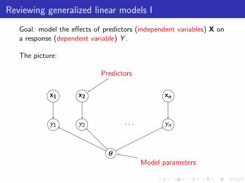
Reviewing generalized linear models I
Goal: model the effects of predictors (independent variables) X ona response (dependent variable) Y .
The picture:
θ
x1
y1
x2
y2
xn
yn· · ·
Predictors
Model parameters
Response
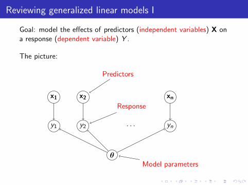
Reviewing generalized linear models I
Goal: model the effects of predictors (independent variables) X ona response (dependent variable) Y .
The picture:
θ
x1
y1
x2
y2
xn
yn· · ·
Predictors
Model parameters
Response
Reviewing generalized linear models I
Goal: model the effects of predictors (independent variables) X ona response (dependent variable) Y .
The picture:
θ
x1
y1
x2
y2
xn
yn· · ·
Predictors
Model parameters
Response
Reviewing generalized linear models I
Goal: model the effects of predictors (independent variables) X ona response (dependent variable) Y .
The picture:
θ
x1
y1
x2
y2
xn
yn· · ·
Predictors
Model parameters
Response
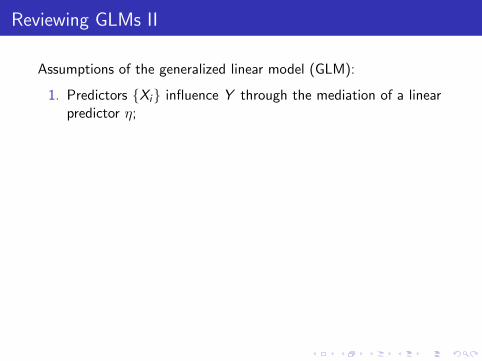
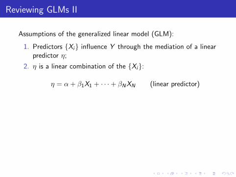
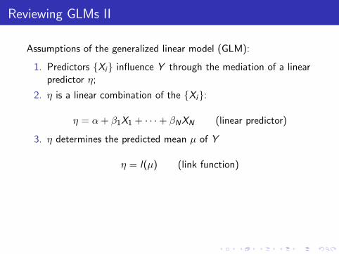
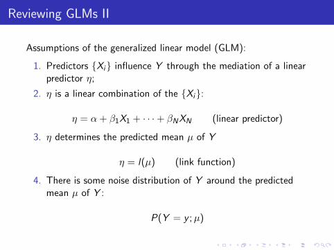
Reviewing GLMs II
Assumptions of the generalized linear model (GLM):
1. Predictors {Xi} influence Y through the mediation of a linearpredictor η;
2. η is a linear combination of the {Xi}:
η = α + β1X1 + · · ·+ βNXN (linear predictor)
3. η determines the predicted mean µ of Y
η = l(µ) (link function)
4. There is some noise distribution of Y around the predictedmean µ of Y :
P(Y = y ;µ)
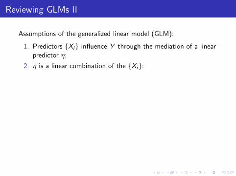
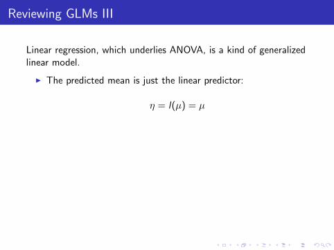
Reviewing GLMs III
Linear regression, which underlies ANOVA, is a kind of generalizedlinear model.
I The predicted mean is just the linear predictor:
η = l(µ) = µ
I Noise is normally (=Gaussian) distributed around 0 withstandard deviation σ:
ε ∼ N(0, σ)
I This gives us the traditional linear regression equation:
Y =
Predicted Mean µ = η︷ ︸︸ ︷α + β1X1 + · · ·+ βnXn +
Noise∼N(0,σ)︷︸︸︷ε
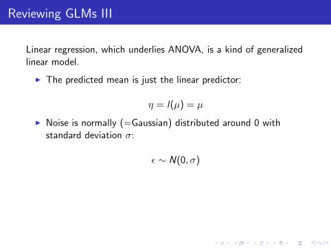
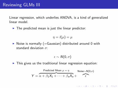

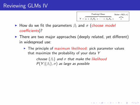
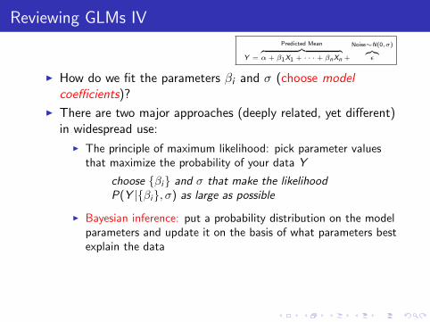
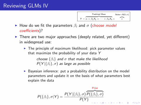
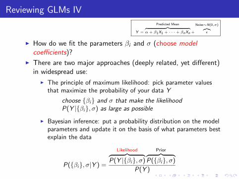
Reviewing GLMs IV
Y =
Predicted Mean︷ ︸︸ ︷α + β1X1 + · · · + βnXn +
Noise∼N(0,σ)︷︸︸︷ε
I How do we fit the parameters βi and σ (choose modelcoefficients)?
I There are two major approaches (deeply related, yet different)in widespread use:
I The principle of maximum likelihood: pick parameter valuesthat maximize the probability of your data Y
choose {βi} and σ that make the likelihoodP(Y |{βi}, σ) as large as possible
I Bayesian inference: put a probability distribution on the modelparameters and update it on the basis of what parameters bestexplain the data
P({βi}, σ|Y ) =P(Y |{βi}, σ)
Prior︷ ︸︸ ︷P({βi}, σ)
P(Y )
Reviewing GLMs IV
Y =
Predicted Mean︷ ︸︸ ︷α + β1X1 + · · · + βnXn +
Noise∼N(0,σ)︷︸︸︷ε
I How do we fit the parameters βi and σ (choose modelcoefficients)?
I There are two major approaches (deeply related, yet different)in widespread use:
I The principle of maximum likelihood: pick parameter valuesthat maximize the probability of your data Y
choose {βi} and σ that make the likelihoodP(Y |{βi}, σ) as large as possible
I Bayesian inference: put a probability distribution on the modelparameters and update it on the basis of what parameters bestexplain the data
P({βi}, σ|Y ) =
Likelihood︷ ︸︸ ︷P(Y |{βi}, σ)
Prior︷ ︸︸ ︷P({βi}, σ)
P(Y )

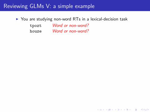
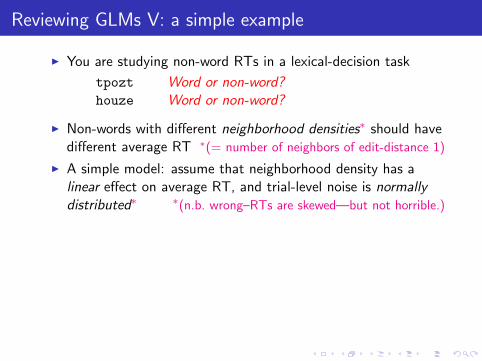
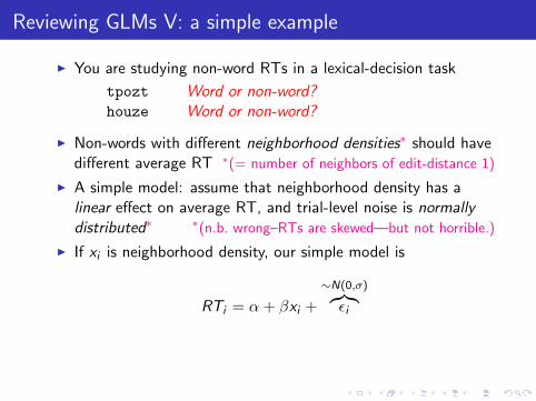
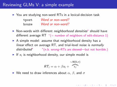
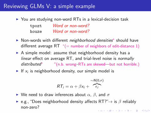
Reviewing GLMs V: a simple example
I You are studying non-word RTs in a lexical-decision task
tpozt Word or non-word?houze Word or non-word?
I Non-words with different neighborhood densities∗ should havedifferent average RT ∗(= number of neighbors of edit-distance 1)
I A simple model: assume that neighborhood density has alinear effect on average RT, and trial-level noise is normallydistributed∗ ∗(n.b. wrong–RTs are skewed—but not horrible.)
I If xi is neighborhood density, our simple model is
RTi = α + βxi +
∼N(0,σ)︷︸︸︷εi
I We need to draw inferences about α, β, and σ
I e.g., “Does neighborhood density affects RT?”→ is β reliablynon-zero?

Reviewing GLMs V: a simple example
I You are studying non-word RTs in a lexical-decision task
tpozt Word or non-word?
houze Word or non-word?
I Non-words with different neighborhood densities∗ should havedifferent average RT ∗(= number of neighbors of edit-distance 1)
I A simple model: assume that neighborhood density has alinear effect on average RT, and trial-level noise is normallydistributed∗ ∗(n.b. wrong–RTs are skewed—but not horrible.)
I If xi is neighborhood density, our simple model is
RTi = α + βxi +
∼N(0,σ)︷︸︸︷εi
I We need to draw inferences about α, β, and σ
I e.g., “Does neighborhood density affects RT?”→ is β reliablynon-zero?
Reviewing GLMs V: a simple example
I You are studying non-word RTs in a lexical-decision task
tpozt Word or non-word?houze Word or non-word?
I Non-words with different neighborhood densities∗ should havedifferent average RT ∗(= number of neighbors of edit-distance 1)
I A simple model: assume that neighborhood density has alinear effect on average RT, and trial-level noise is normallydistributed∗ ∗(n.b. wrong–RTs are skewed—but not horrible.)
I If xi is neighborhood density, our simple model is
RTi = α + βxi +
∼N(0,σ)︷︸︸︷εi
I We need to draw inferences about α, β, and σ
I e.g., “Does neighborhood density affects RT?”→ is β reliablynon-zero?
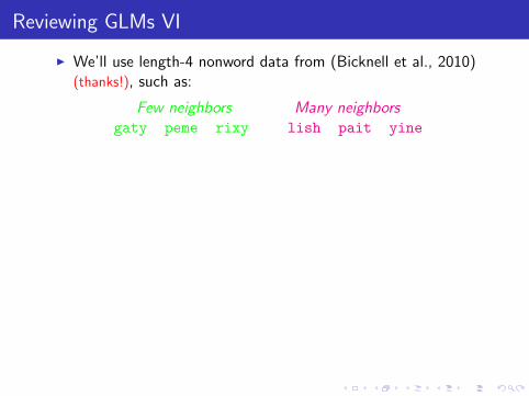
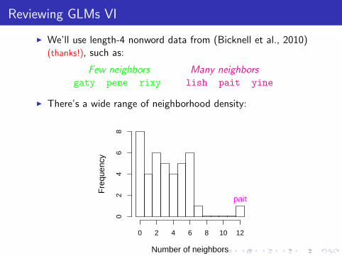
Reviewing GLMs VI
I We’ll use length-4 nonword data from (Bicknell et al., 2010)(thanks!), such as:
Few neighbors Many neighborsgaty peme rixy lish pait yine
I There’s a wide range of neighborhood density:
Number of neighbors
Fre
quen
cy
0 2 4 6 8 10 12
02
46
8
pait
Reviewing GLMs VI
I We’ll use length-4 nonword data from (Bicknell et al., 2010)(thanks!), such as:
Few neighbors Many neighborsgaty peme rixy lish pait yine
I There’s a wide range of neighborhood density:
Number of neighbors
Fre
quen
cy
0 2 4 6 8 10 12
02
46
8
pait
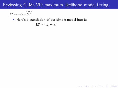
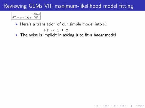
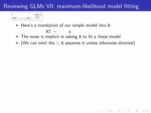
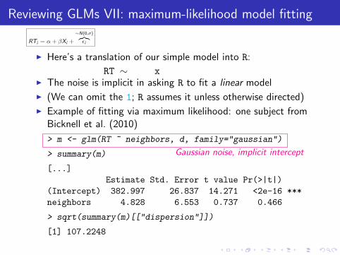
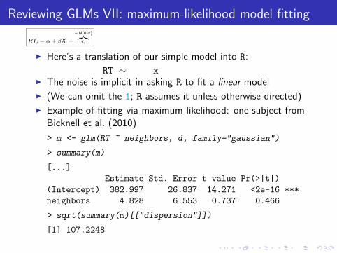
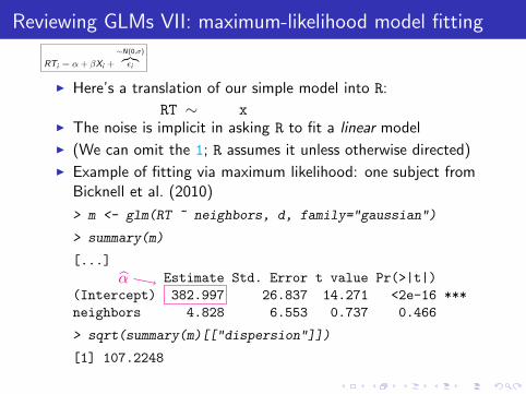
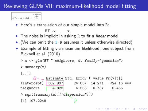
Reviewing GLMs VII: maximum-likelihood model fitting
RTi = α + βXi +
∼N(0,σ)︷︸︸︷εi
I Here’s a translation of our simple model into R:
RT ∼ 1 + x
I The noise is implicit in asking R to fit a linear model
I (We can omit the 1; R assumes it unless otherwise directed)
I Example of fitting via maximum likelihood: one subject fromBicknell et al. (2010)
> m <- glm(RT ~ neighbors, d, family="gaussian")
> summary(m)
[...]
Estimate Std. Error t value Pr(>|t|)
(Intercept) 382.997 26.837 14.271 <2e-16 ***
neighbors 4.828 6.553 0.737 0.466
> sqrt(summary(m)[["dispersion"]])
[1] 107.2248
Gaussian noise, implicit intercept
α̂
β̂
σ̂
Reviewing GLMs VII: maximum-likelihood model fitting
RTi = α + βXi +
∼N(0,σ)︷︸︸︷εi
I Here’s a translation of our simple model into R:
RT ∼ 1 + xI The noise is implicit in asking R to fit a linear model
I (We can omit the 1; R assumes it unless otherwise directed)
I Example of fitting via maximum likelihood: one subject fromBicknell et al. (2010)
> m <- glm(RT ~ neighbors, d, family="gaussian")
> summary(m)
[...]
Estimate Std. Error t value Pr(>|t|)
(Intercept) 382.997 26.837 14.271 <2e-16 ***
neighbors 4.828 6.553 0.737 0.466
> sqrt(summary(m)[["dispersion"]])
[1] 107.2248
Gaussian noise, implicit intercept
α̂
β̂
σ̂
Reviewing GLMs VII: maximum-likelihood model fitting
RTi = α + βXi +
∼N(0,σ)︷︸︸︷εi
I Here’s a translation of our simple model into R:
RT ∼ xI The noise is implicit in asking R to fit a linear model
I (We can omit the 1; R assumes it unless otherwise directed)
I Example of fitting via maximum likelihood: one subject fromBicknell et al. (2010)
> m <- glm(RT ~ neighbors, d, family="gaussian")
> summary(m)
[...]
Estimate Std. Error t value Pr(>|t|)
(Intercept) 382.997 26.837 14.271 <2e-16 ***
neighbors 4.828 6.553 0.737 0.466
> sqrt(summary(m)[["dispersion"]])
[1] 107.2248
Gaussian noise, implicit intercept
α̂
β̂
σ̂
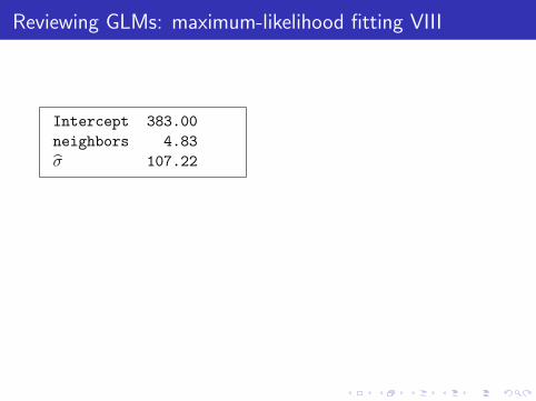
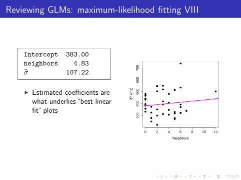
Reviewing GLMs: maximum-likelihood fitting VIII
Intercept 383.00
neighbors 4.83
σ̂ 107.22
I Estimated coefficients arewhat underlies “best linearfit” plots
●
●
●
●
●●
●
●
●
●
●
●
●
●
●
●
●
●
●
●●
●
●
●
●
●
●
●
●
●
●
●
●
●
●
●
●
●
●
●
0 2 4 6 8 10 12
300
400
500
600
700
Neighbors
RT
(m
s)
Reviewing GLMs: maximum-likelihood fitting VIII
Intercept 383.00
neighbors 4.83
σ̂ 107.22
I Estimated coefficients arewhat underlies “best linearfit” plots
●
●
●
●
●●
●
●
●
●
●
●
●
●
●
●
●
●
●
●●
●
●
●
●
●
●
●
●
●
●
●
●
●
●
●
●
●
●
●
0 2 4 6 8 10 12
300
400
500
600
700
Neighbors
RT
(m
s)
Reviewing GLMs: maximum-likelihood fitting VIII
Intercept 383.00
neighbors 4.83
σ̂ 107.22
I Estimated coefficients arewhat underlies “best linearfit” plots
●
●
●
●
●●
●
●
●
●
●
●
●
●
●
●
●
●
●
●●
●
●
●
●
●
●
●
●
●
●
●
●
●
●
●
●
●
●
●
0 2 4 6 8 10 1230
040
050
060
070
0Neighbors
RT
(m
s)
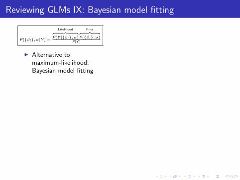
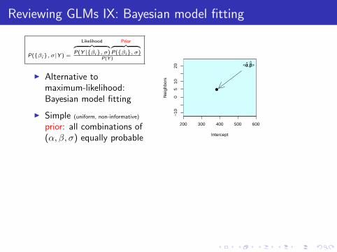
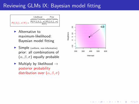
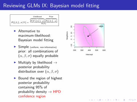
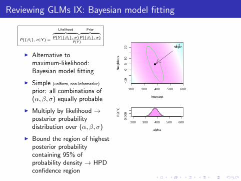
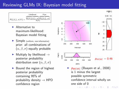
Reviewing GLMs IX: Bayesian model fitting
P({βi}, σ|Y ) =
Likelihood︷ ︸︸ ︷P(Y |{βi}, σ)
Prior︷ ︸︸ ︷P({βi}, σ)
P(Y )
I Alternative tomaximum-likelihood:Bayesian model fitting
I Simple (uniform, non-informative)
prior: all combinations of(α, β, σ) equally probable
I Multiply by likelihood →posterior probabilitydistribution over (α, β, σ)
I Bound the region of highestposterior probabilitycontaining 95% ofprobability density → HPDconfidence region
−10
−5
0
5
10
15
20
25
0.00 0.06
P(ββ|Y)
ββ
pMCMC = 0.46
200 300 400 500 600
−10
05
1020
Intercept
Nei
ghbo
rs
●
<αα̂,ββ̂>
200 300 400 500 600
−10
05
1020
Intercept
Nei
ghbo
rs
●
<αα̂,ββ̂>
200 300 400 500 600
−10
05
1020
Intercept
Nei
ghbo
rs
●
<αα̂,ββ̂>
200 300 400 500 600
0.00
0
alpha
P(αα
|Y)
I pMCMC (Baayen et al., 2008)is 1 minus the largestpossible symmetricconfidence interval wholly onone side of 0
Reviewing GLMs IX: Bayesian model fitting
P({βi}, σ|Y ) =
Likelihood︷ ︸︸ ︷P(Y |{βi}, σ)
Prior︷ ︸︸ ︷P({βi}, σ)
P(Y )
I Alternative tomaximum-likelihood:Bayesian model fitting
I Simple (uniform, non-informative)
prior: all combinations of(α, β, σ) equally probable
I Multiply by likelihood →posterior probabilitydistribution over (α, β, σ)
I Bound the region of highestposterior probabilitycontaining 95% ofprobability density → HPDconfidence region
−10
−5
0
5
10
15
20
25
0.00 0.06
P(ββ|Y)
ββ
pMCMC = 0.46
200 300 400 500 600
−10
05
1020
Intercept
Nei
ghbo
rs
●
<αα̂,ββ̂>
200 300 400 500 600
−10
05
1020
Intercept
Nei
ghbo
rs
●
<αα̂,ββ̂>
200 300 400 500 600
−10
05
1020
Intercept
Nei
ghbo
rs
●
<αα̂,ββ̂>
200 300 400 500 6000.
000
alpha
P(αα
|Y)
I pMCMC (Baayen et al., 2008)is 1 minus the largestpossible symmetricconfidence interval wholly onone side of 0
Multi-level Models
I But of course experiments don’t have just one participant
I Different participants may have different idiosyncratic behavior
I And items may have idiosyncratic properties too
I We’d like to take these into account, and perhaps investigatethem directly too.
I This is what multi-level (hierarchical, mixed-effects) models arefor!
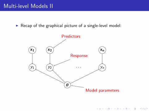
Multi-level Models II
I Recap of the graphical picture of a single-level model:
θ
x1
y1
x2
y2
xn
yn· · ·
Predictors
Model parameters
Response
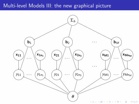
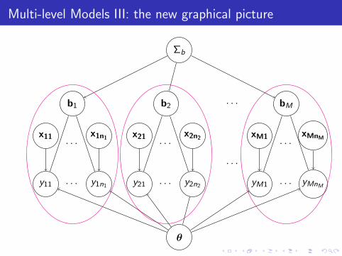
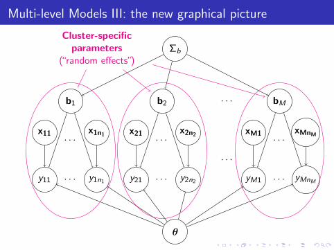
Multi-level Models III: the new graphical picture
θ
Σb
b1 b2 bM· · ·
· · ·
x11 x1n1
y11 y1n1
· · ·
· · ·
x21 x2n2
y21 y2n2
· · ·
· · ·
xM1 xMnM
yM1 yMnM
· · ·
· · ·
Cluster-specificparameters
(“random effects”)
Shared parameters(“fixed effects”)
Parameters governinginter-cluster variability
Multi-level Models III: the new graphical picture
θ
Σb
b1 b2 bM· · ·
· · ·
x11 x1n1
y11 y1n1
· · ·
· · ·
x21 x2n2
y21 y2n2
· · ·
· · ·
xM1 xMnM
yM1 yMnM
· · ·
· · ·
Cluster-specificparameters
(“random effects”)
Shared parameters(“fixed effects”)
Parameters governinginter-cluster variability
Multi-level Models III: the new graphical picture
θ
Σb
b1 b2 bM· · ·
· · ·
x11 x1n1
y11 y1n1
· · ·
· · ·
x21 x2n2
y21 y2n2
· · ·
· · ·
xM1 xMnM
yM1 yMnM
· · ·
· · ·
Cluster-specificparameters
(“random effects”)
Shared parameters(“fixed effects”)
Parameters governinginter-cluster variability
Multi-level Models III: the new graphical picture
θ
Σb
b1 b2 bM· · ·
· · ·
x11 x1n1
y11 y1n1
· · ·
· · ·
x21 x2n2
y21 y2n2
· · ·
· · ·
xM1 xMnM
yM1 yMnM
· · ·
· · ·
Cluster-specificparameters
(“random effects”)
Shared parameters(“fixed effects”)
Parameters governinginter-cluster variability
Multi-level Models III: the new graphical picture
θ
Σb
b1 b2 bM· · ·
· · ·
x11 x1n1
y11 y1n1
· · ·
· · ·
x21 x2n2
y21 y2n2
· · ·
· · ·
xM1 xMnM
yM1 yMnM
· · ·
· · ·
Cluster-specificparameters
(“random effects”)
Shared parameters(“fixed effects”)
Parameters governinginter-cluster variability
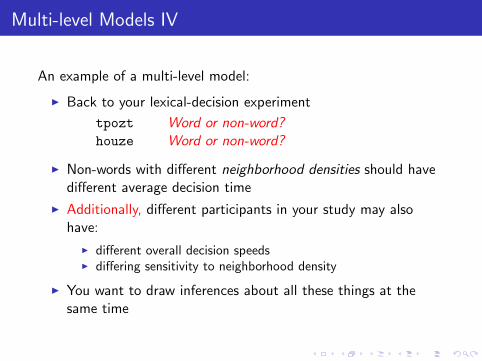
Multi-level Models IV
An example of a multi-level model:
I Back to your lexical-decision experiment
tpozt Word or non-word?houze Word or non-word?
I Non-words with different neighborhood densities should havedifferent average decision time
I Additionally, different participants in your study may alsohave:
I different overall decision speedsI differing sensitivity to neighborhood density
I You want to draw inferences about all these things at thesame time
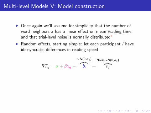
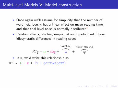
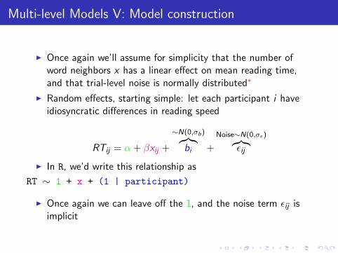
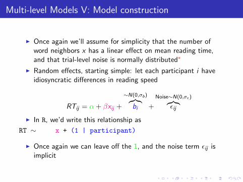
Multi-level Models V: Model construction
I Once again we’ll assume for simplicity that the number ofword neighbors x has a linear effect on mean reading time,and that trial-level noise is normally distributed∗
I Random effects, starting simple: let each participant i haveidiosyncratic differences in reading speed
RTij = α + βxij +
∼N(0,σb)︷︸︸︷bi +
Noise∼N(0,σε)︷︸︸︷εij
I In R, we’d write this relationship as
I Once again we can leave off the 1, and the noise term εij isimplicit
Multi-level Models V: Model construction
I Once again we’ll assume for simplicity that the number ofword neighbors x has a linear effect on mean reading time,and that trial-level noise is normally distributed∗
I Random effects, starting simple: let each participant i haveidiosyncratic differences in reading speed
RTij = α + βxij +
∼N(0,σb)︷︸︸︷bi +
Noise∼N(0,σε)︷︸︸︷εij
I In R, we’d write this relationship as
RT ∼ 1 + x + (1 | participant)
I Once again we can leave off the 1, and the noise term εij isimplicit
Multi-level Models V: Model construction
I Once again we’ll assume for simplicity that the number ofword neighbors x has a linear effect on mean reading time,and that trial-level noise is normally distributed∗
I Random effects, starting simple: let each participant i haveidiosyncratic differences in reading speed
RTij = α + βxij +
∼N(0,σb)︷︸︸︷bi +
Noise∼N(0,σε)︷︸︸︷εij
I In R, we’d write this relationship as
RT ∼ x + (1 | participant)
I Once again we can leave off the 1, and the noise term εij isimplicit
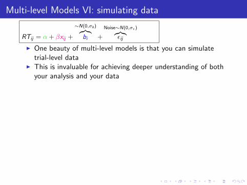
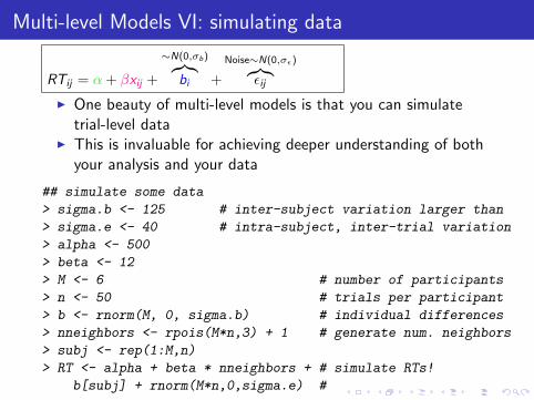
Multi-level Models VI: simulating data
RTij = α + βxij +
∼N(0,σb)︷︸︸︷bi +
Noise∼N(0,σε)︷︸︸︷εij
I One beauty of multi-level models is that you can simulatetrial-level data
I This is invaluable for achieving deeper understanding of bothyour analysis and your data
## simulate some data
> sigma.b <- 125 # inter-subject variation larger than
> sigma.e <- 40 # intra-subject, inter-trial variation
> alpha <- 500
> beta <- 12
> M <- 6 # number of participants
> n <- 50 # trials per participant
> b <- rnorm(M, 0, sigma.b) # individual differences
> nneighbors <- rpois(M*n,3) + 1 # generate num. neighbors
> subj <- rep(1:M,n)
> RT <- alpha + beta * nneighbors + # simulate RTs!
b[subj] + rnorm(M*n,0,sigma.e) #
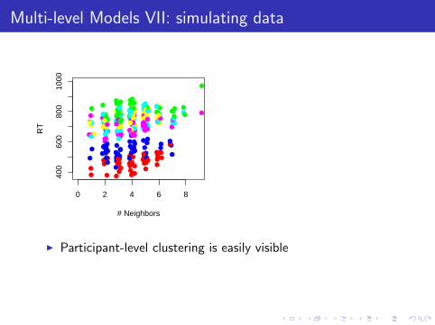
Multi-level Models VII: simulating data
●
●
●
●
●
●
●
●
●
●
●
●
●
●●
●
●
●
●
●
●
●
●
●
●
●
●
●
●
●
●
●
●
●
●
●
●
●●
●
●
●
●
● ●
●
●
●
●
●●
●
●
●
●
●●
●
●
●
●
●● ●
●
●
●
●●
●
●
●
●
●●
●
●
●
●
●●
●
●
●
●
●
●●
●
●●
●
●
●
●●
●
●●
●
●
●
●
●
●
●
●
●
●
●
●●
●
●
●
●
●
●
●
●
●
●
●
●
●
●
●
●
●
●●
●
●
●
●
●
●
●
●
●
●
●
●●
●
●●
●
●
●
●
●
●
●
●
●
●
● ●●
●
●
●
●
●●
●
●
●
●● ●
●
●
●
●
●
●
●
●
●
●
●
●
●
●
●
●
●●
●
●
●
●
●
●
●
●
●
●
●
●
●
●
●
●●●
●
●
●
●
●●
●
●
●
●
●
●
●
●
●
●
●
●
●
●
●
●●
●
●
●
●
●
●
●
●
●
●
●
●
●
●
●
●
●
●
●
●
●
●
●
●
●●
●
●
●●
●
●
●
●
●
●●
●
●
●
●●
●
●
●
●
●
●
●
●
●
●
●
●●
●
●
●
●
●●
●
●
●
●
●
●
●
●
0 2 4 6 8
400
600
800
1000
# Neighbors
RT
I Participant-level clustering is easily visible
I This reflects the fact that inter-participant variation (125ms)is larger than inter-trial variation (40ms)
I And the effects of neighborhood density are also visible
Multi-level Models VII: simulating data
●
●
●
●
●
●
●
●
●
●
●
●
●
●●
●
●
●
●
●
●
●
●
●
●
●
●
●
●
●
●
●
●
●
●
●
●
●●
●
●
●
●
● ●
●
●
●
●
●●
●
●
●
●
●●
●
●
●
●
●● ●
●
●
●
●●
●
●
●
●
●●
●
●
●
●
●●
●
●
●
●
●
●●
●
●●
●
●
●
●●
●
●●
●
●
●
●
●
●
●
●
●
●
●
●●
●
●
●
●
●
●
●
●
●
●
●
●
●
●
●
●
●
●●
●
●
●
●
●
●
●
●
●
●
●
●●
●
●●
●
●
●
●
●
●
●
●
●
●
● ●●
●
●
●
●
●●
●
●
●
●● ●
●
●
●
●
●
●
●
●
●
●
●
●
●
●
●
●
●●
●
●
●
●
●
●
●
●
●
●
●
●
●
●
●
●●●
●
●
●
●
●●
●
●
●
●
●
●
●
●
●
●
●
●
●
●
●
●●
●
●
●
●
●
●
●
●
●
●
●
●
●
●
●
●
●
●
●
●
●
●
●
●
●●
●
●
●●
●
●
●
●
●
●●
●
●
●
●●
●
●
●
●
●
●
●
●
●
●
●
●●
●
●
●
●
●●
●
●
●
●
●
●
●
●
0 2 4 6 8
400
600
800
1000
# Neighbors
RT
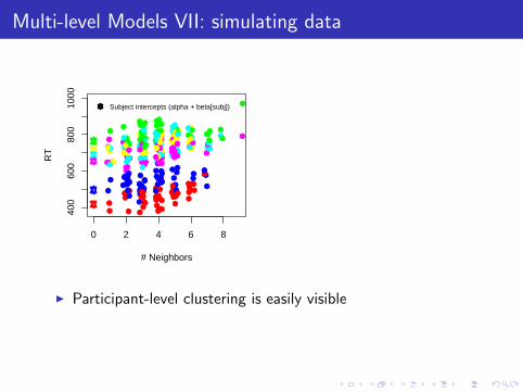
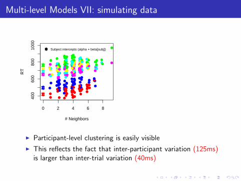
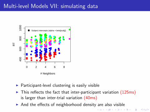
Subject intercepts (alpha + beta[subj])
I Participant-level clustering is easily visible
I This reflects the fact that inter-participant variation (125ms)is larger than inter-trial variation (40ms)
I And the effects of neighborhood density are also visible
Multi-level Models VII: simulating data
●
●
●
●
●
●
●
●
●
●
●
●
●
●●
●
●
●
●
●
●
●
●
●
●
●
●
●
●
●
●
●
●
●
●
●
●
●●
●
●
●
●
● ●
●
●
●
●
●●
●
●
●
●
●●
●
●
●
●
●● ●
●
●
●
●●
●
●
●
●
●●
●
●
●
●
●●
●
●
●
●
●
●●
●
●●
●
●
●
●●
●
●●
●
●
●
●
●
●
●
●
●
●
●
●●
●
●
●
●
●
●
●
●
●
●
●
●
●
●
●
●
●
●●
●
●
●
●
●
●
●
●
●
●
●
●●
●
●●
●
●
●
●
●
●
●
●
●
●
● ●●
●
●
●
●
●●
●
●
●
●● ●
●
●
●
●
●
●
●
●
●
●
●
●
●
●
●
●
●●
●
●
●
●
●
●
●
●
●
●
●
●
●
●
●
●●●
●
●
●
●
●●
●
●
●
●
●
●
●
●
●
●
●
●
●
●
●
●●
●
●
●
●
●
●
●
●
●
●
●
●
●
●
●
●
●
●
●
●
●
●
●
●
●●
●
●
●●
●
●
●
●
●
●●
●
●
●
●●
●
●
●
●
●
●
●
●
●
●
●
●●
●
●
●
●
●●
●
●
●
●
●
●
●
●
0 2 4 6 8
400
600
800
1000
# Neighbors
RT
Subject intercepts (alpha + beta[subj])
I Participant-level clustering is easily visible
I This reflects the fact that inter-participant variation (125ms)is larger than inter-trial variation (40ms)
I And the effects of neighborhood density are also visible
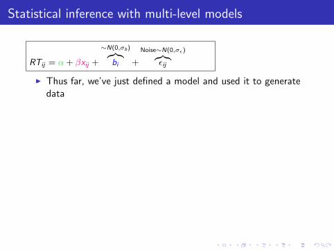
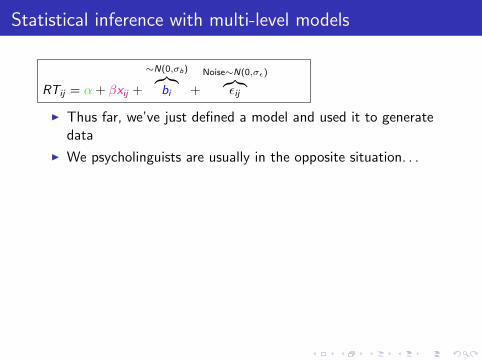
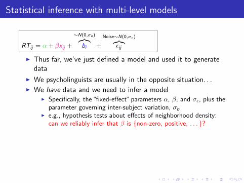
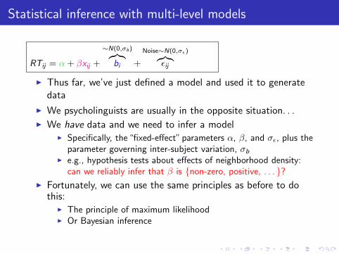
Statistical inference with multi-level models
RTij = α + βxij +
∼N(0,σb)︷︸︸︷bi +
Noise∼N(0,σε)︷︸︸︷εij
I Thus far, we’ve just defined a model and used it to generatedata
I We psycholinguists are usually in the opposite situation. . .I We have data and we need to infer a model
I Specifically, the “fixed-effect” parameters α, β, and σε, plus theparameter governing inter-subject variation, σb
I e.g., hypothesis tests about effects of neighborhood density:can we reliably infer that β is {non-zero, positive, . . . }?
I Fortunately, we can use the same principles as before to dothis:
I The principle of maximum likelihoodI Or Bayesian inference
Statistical inference with multi-level models
RTij = α + βxij +
∼N(0,σb)︷︸︸︷bi +
Noise∼N(0,σε)︷︸︸︷εij
I Thus far, we’ve just defined a model and used it to generatedata
I We psycholinguists are usually in the opposite situation. . .
I We have data and we need to infer a modelI Specifically, the “fixed-effect” parameters α, β, and σε, plus the
parameter governing inter-subject variation, σbI e.g., hypothesis tests about effects of neighborhood density:
can we reliably infer that β is {non-zero, positive, . . . }?I Fortunately, we can use the same principles as before to do
this:I The principle of maximum likelihoodI Or Bayesian inference
Statistical inference with multi-level models
RTij = α + βxij +
∼N(0,σb)︷︸︸︷bi +
Noise∼N(0,σε)︷︸︸︷εij
I Thus far, we’ve just defined a model and used it to generatedata
I We psycholinguists are usually in the opposite situation. . .I We have data and we need to infer a model
I Specifically, the “fixed-effect” parameters α, β, and σε, plus theparameter governing inter-subject variation, σb
I e.g., hypothesis tests about effects of neighborhood density:can we reliably infer that β is {non-zero, positive, . . . }?
I Fortunately, we can use the same principles as before to dothis:
I The principle of maximum likelihoodI Or Bayesian inference
Statistical inference with multi-level models
RTij = α + βxij +
∼N(0,σb)︷︸︸︷bi +
Noise∼N(0,σε)︷︸︸︷εij
I Thus far, we’ve just defined a model and used it to generatedata
I We psycholinguists are usually in the opposite situation. . .I We have data and we need to infer a model
I Specifically, the “fixed-effect” parameters α, β, and σε, plus theparameter governing inter-subject variation, σb
I e.g., hypothesis tests about effects of neighborhood density:can we reliably infer that β is {non-zero, positive, . . . }?
I Fortunately, we can use the same principles as before to dothis:
I The principle of maximum likelihoodI Or Bayesian inference
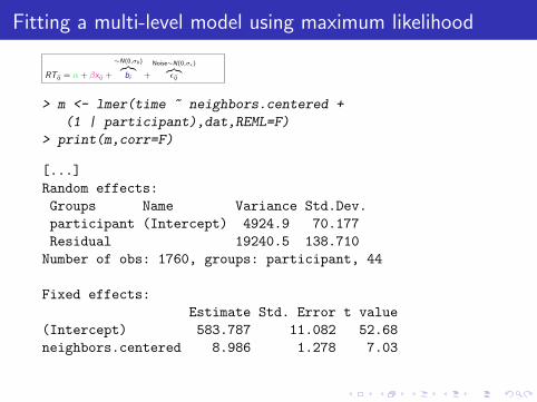
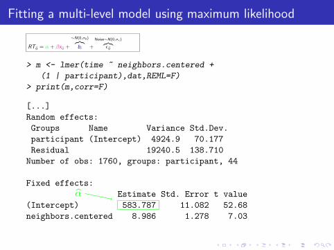
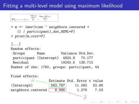
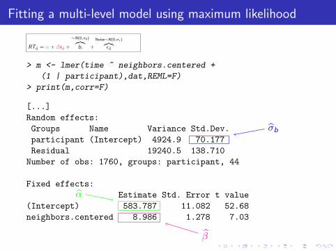
Fitting a multi-level model using maximum likelihood
RTij = α + βxij +
∼N(0,σb)︷︸︸︷bi +
Noise∼N(0,σε)︷︸︸︷εij
> m <- lmer(time ~ neighbors.centered +
(1 | participant),dat,REML=F)
> print(m,corr=F)
[...]
Random effects:
Groups Name Variance Std.Dev.
participant (Intercept) 4924.9 70.177
Residual 19240.5 138.710
Number of obs: 1760, groups: participant, 44
Fixed effects:
Estimate Std. Error t value
(Intercept) 583.787 11.082 52.68
neighbors.centered 8.986 1.278 7.03
α̂
β̂
σ̂b
σ̂ε
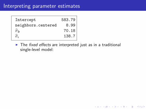
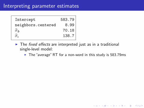
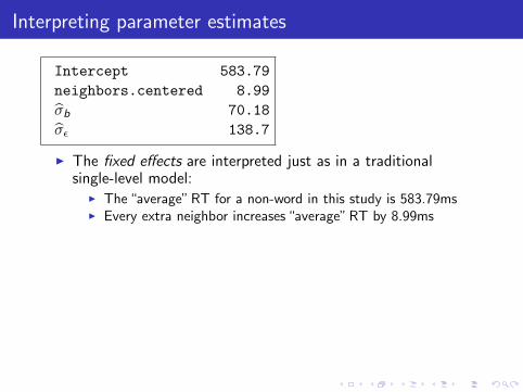
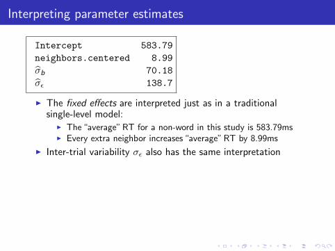
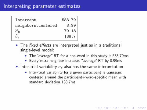
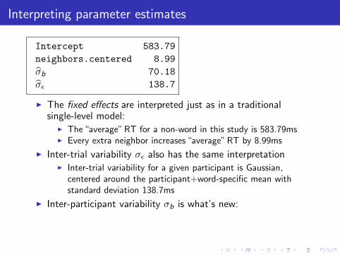
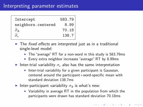
Interpreting parameter estimates
Intercept 583.79
neighbors.centered 8.99
σ̂b 70.18
σ̂ε 138.7
I The fixed effects are interpreted just as in a traditionalsingle-level model:
I The “average” RT for a non-word in this study is 583.79msI Every extra neighbor increases “average” RT by 8.99ms
I Inter-trial variability σε also has the same interpretationI Inter-trial variability for a given participant is Gaussian,
centered around the participant+word-specific mean withstandard deviation 138.7ms
I Inter-participant variability σb is what’s new:I Variability in average RT in the population from which the
participants were drawn has standard deviation 70.18ms
Interpreting parameter estimates
Intercept 583.79
neighbors.centered 8.99
σ̂b 70.18
σ̂ε 138.7
I The fixed effects are interpreted just as in a traditionalsingle-level model:
I The “average” RT for a non-word in this study is 583.79ms
I Every extra neighbor increases “average” RT by 8.99ms
I Inter-trial variability σε also has the same interpretationI Inter-trial variability for a given participant is Gaussian,
centered around the participant+word-specific mean withstandard deviation 138.7ms
I Inter-participant variability σb is what’s new:I Variability in average RT in the population from which the
participants were drawn has standard deviation 70.18ms
Interpreting parameter estimates
Intercept 583.79
neighbors.centered 8.99
σ̂b 70.18
σ̂ε 138.7
I The fixed effects are interpreted just as in a traditionalsingle-level model:
I The “average” RT for a non-word in this study is 583.79msI Every extra neighbor increases “average” RT by 8.99ms
I Inter-trial variability σε also has the same interpretationI Inter-trial variability for a given participant is Gaussian,
centered around the participant+word-specific mean withstandard deviation 138.7ms
I Inter-participant variability σb is what’s new:I Variability in average RT in the population from which the
participants were drawn has standard deviation 70.18ms
Interpreting parameter estimates
Intercept 583.79
neighbors.centered 8.99
σ̂b 70.18
σ̂ε 138.7
I The fixed effects are interpreted just as in a traditionalsingle-level model:
I The “average” RT for a non-word in this study is 583.79msI Every extra neighbor increases “average” RT by 8.99ms
I Inter-trial variability σε also has the same interpretation
I Inter-trial variability for a given participant is Gaussian,centered around the participant+word-specific mean withstandard deviation 138.7ms
I Inter-participant variability σb is what’s new:I Variability in average RT in the population from which the
participants were drawn has standard deviation 70.18ms
Interpreting parameter estimates
Intercept 583.79
neighbors.centered 8.99
σ̂b 70.18
σ̂ε 138.7
I The fixed effects are interpreted just as in a traditionalsingle-level model:
I The “average” RT for a non-word in this study is 583.79msI Every extra neighbor increases “average” RT by 8.99ms
I Inter-trial variability σε also has the same interpretationI Inter-trial variability for a given participant is Gaussian,
centered around the participant+word-specific mean withstandard deviation 138.7ms
I Inter-participant variability σb is what’s new:I Variability in average RT in the population from which the
participants were drawn has standard deviation 70.18ms
Interpreting parameter estimates
Intercept 583.79
neighbors.centered 8.99
σ̂b 70.18
σ̂ε 138.7
I The fixed effects are interpreted just as in a traditionalsingle-level model:
I The “average” RT for a non-word in this study is 583.79msI Every extra neighbor increases “average” RT by 8.99ms
I Inter-trial variability σε also has the same interpretationI Inter-trial variability for a given participant is Gaussian,
centered around the participant+word-specific mean withstandard deviation 138.7ms
I Inter-participant variability σb is what’s new:
I Variability in average RT in the population from which theparticipants were drawn has standard deviation 70.18ms
Interpreting parameter estimates
Intercept 583.79
neighbors.centered 8.99
σ̂b 70.18
σ̂ε 138.7
I The fixed effects are interpreted just as in a traditionalsingle-level model:
I The “average” RT for a non-word in this study is 583.79msI Every extra neighbor increases “average” RT by 8.99ms
I Inter-trial variability σε also has the same interpretationI Inter-trial variability for a given participant is Gaussian,
centered around the participant+word-specific mean withstandard deviation 138.7ms
I Inter-participant variability σb is what’s new:I Variability in average RT in the population from which the
participants were drawn has standard deviation 70.18ms
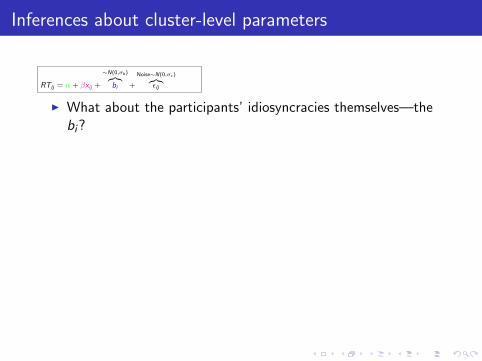
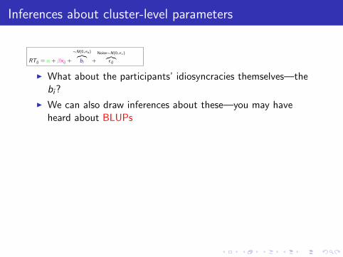
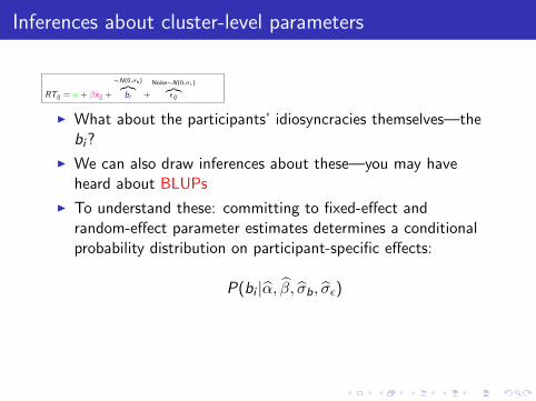
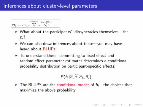
Inferences about cluster-level parameters
RTij = α + βxij +
∼N(0,σb)︷︸︸︷bi +
Noise∼N(0,σε)︷︸︸︷εij
I What about the participants’ idiosyncracies themselves—thebi?
I We can also draw inferences about these—you may haveheard about BLUPs
I To understand these: committing to fixed-effect andrandom-effect parameter estimates determines a conditionalprobability distribution on participant-specific effects:
P(bi |α̂, β̂, σ̂b, σ̂ε)
I The BLUPS are the conditional modes of bi—the choices thatmaximize the above probability
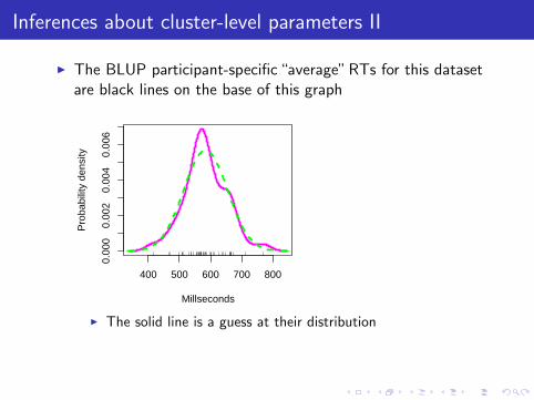
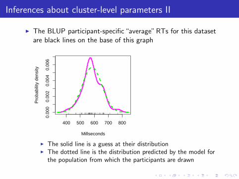
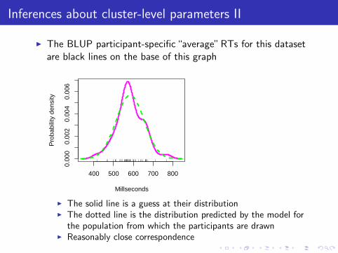
Inferences about cluster-level parameters II
I The BLUP participant-specific “average” RTs for this datasetare black lines on the base of this graph
400 500 600 700 800
0.00
00.
002
0.00
40.
006
Millseconds
Pro
babi
lity
dens
ity
I The solid line is a guess at their distribution
I The dotted line is the distribution predicted by the model forthe population from which the participants are drawn
I Reasonably close correspondence
Inferences about cluster-level parameters II
I The BLUP participant-specific “average” RTs for this datasetare black lines on the base of this graph
400 500 600 700 800
0.00
00.
002
0.00
40.
006
Millseconds
Pro
babi
lity
dens
ity
I The solid line is a guess at their distributionI The dotted line is the distribution predicted by the model for
the population from which the participants are drawn
I Reasonably close correspondence
Inferences about cluster-level parameters II
I The BLUP participant-specific “average” RTs for this datasetare black lines on the base of this graph
400 500 600 700 800
0.00
00.
002
0.00
40.
006
Millseconds
Pro
babi
lity
dens
ity
I The solid line is a guess at their distributionI The dotted line is the distribution predicted by the model for
the population from which the participants are drawnI Reasonably close correspondence
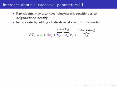
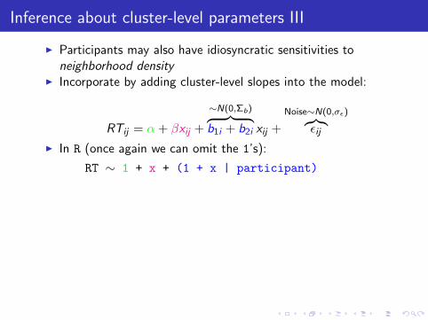
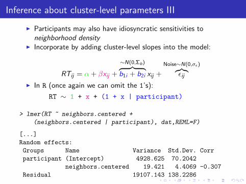
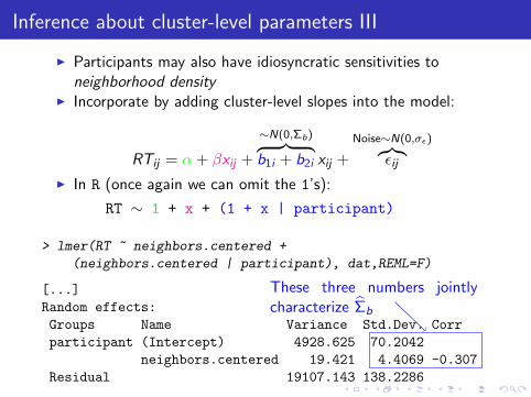
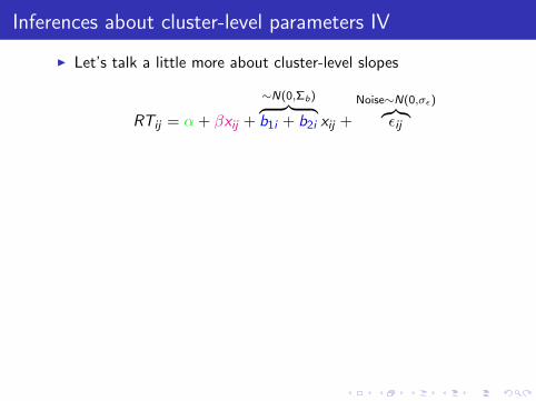
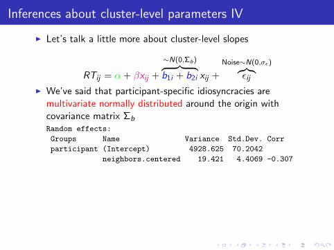
Inference about cluster-level parameters III
I Participants may also have idiosyncratic sensitivities toneighborhood density
I Incorporate by adding cluster-level slopes into the model:
RTij = α + βxij +
∼N(0,Σb)︷ ︸︸ ︷b1i + b2i xij +
Noise∼N(0,σε)︷︸︸︷εij
I In R (once again we can omit the 1’s):
RT ∼ 1 + x + (1 + x | participant)
> lmer(RT ~ neighbors.centered +
(neighbors.centered | participant), dat,REML=F)
[...]
Random effects:
Groups Name Variance Std.Dev. Corr
participant (Intercept) 4928.625 70.2042
neighbors.centered 19.421 4.4069 -0.307
Residual 19107.143 138.2286
These three numbers jointlycharacterize Σ̂b
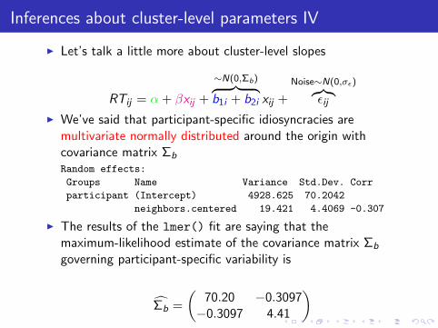
Inferences about cluster-level parameters IV
I Let’s talk a little more about cluster-level slopes
RTij = α + βxij +
∼N(0,Σb)︷ ︸︸ ︷b1i + b2i xij +
Noise∼N(0,σε)︷︸︸︷εij
I We’ve said that participant-specific idiosyncracies aremultivariate normally distributed around the origin withcovariance matrix Σb
Random effects:
Groups Name Variance Std.Dev. Corr
participant (Intercept) 4928.625 70.2042
neighbors.centered 19.421 4.4069 -0.307
I The results of the lmer() fit are saying that themaximum-likelihood estimate of the covariance matrix Σb
governing participant-specific variability is
Σ̂b =
(70.20 −0.3097−0.3097 4.41
)
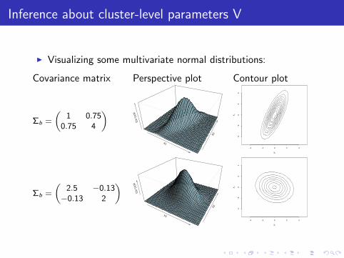
Inference about cluster-level parameters V
I Visualizing some multivariate normal distributions:
Covariance matrix Perspective plot Contour plot
Σb =
(1 0.75
0.75 4
)X1
X2
p(X1,X
2)
X1
X2
0.01
0.02
0.03
0.05
0.07
0.09
0.1
1
−4 −2 0 2 4
−4
−2
02
4
Σb =
(2.5 −0.13−0.13 2
)X1
X2
p(X1,X
2)
X1
X2
0.01
0.02
0.03
0.04
0.06
0.07
−4 −2 0 2 4
−4
−2
02
4
Inference about cluster-level parameters VI
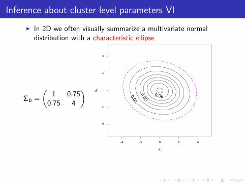
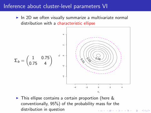
I In 2D we often visually summarize a multivariate normaldistribution with a characteristic ellipse
Σb =
(1 0.75
0.75 4
)
X1
X2
0.01 0.03
0.06
−4 −2 0 2 4
−4
−2
02
4
I This ellipse contains a certain proportion (here &conventionally, 95%) of the probability mass for thedistribution in question
Inference about cluster-level parameters VI
I In 2D we often visually summarize a multivariate normaldistribution with a characteristic ellipse
Σb =
(1 0.75
0.75 4
)
X1
X2
0.01 0.03
0.06
−4 −2 0 2 4
−4
−2
02
4
I This ellipse contains a certain proportion (here &conventionally, 95%) of the probability mass for thedistribution in question
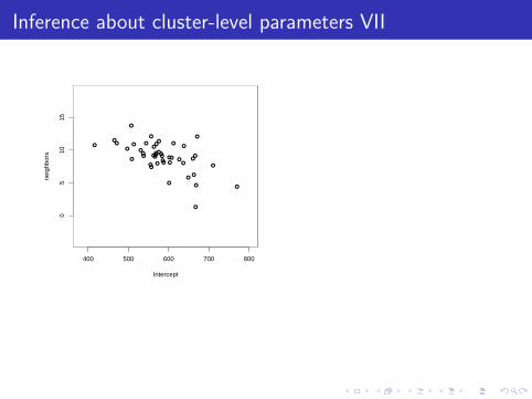
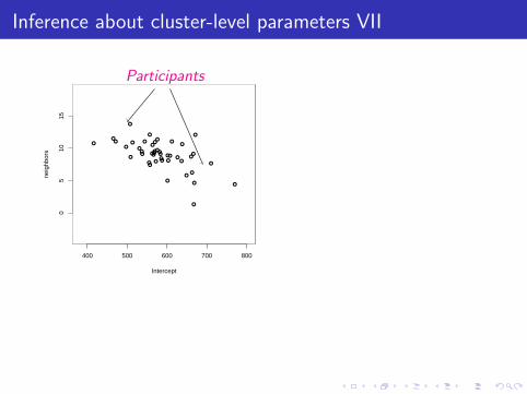
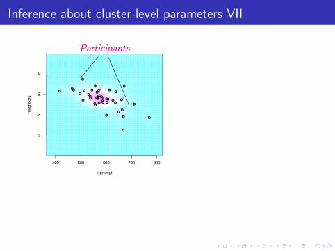
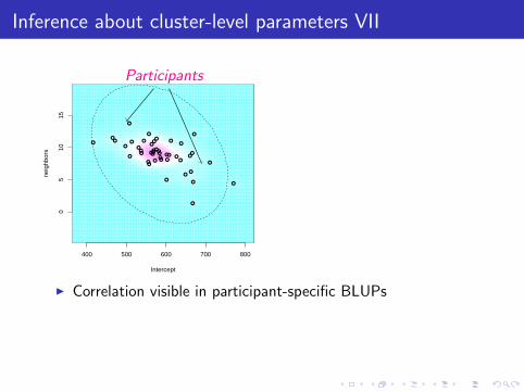
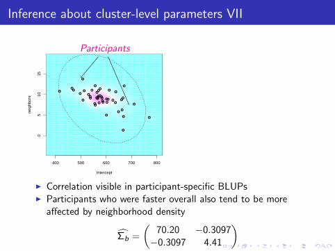
Inference about cluster-level parameters VII
400 500 600 700 800
05
1015
Intercept
neig
hbor
s
●
●●
●
●
●
● ●
●
●●
●
●
●
●
●
●
●●
●●
●●●
●
●●
●●
●
●
●
●
●●
●
●
●
●
●●
●
●
●
Participants
I Correlation visible in participant-specific BLUPsI Participants who were faster overall also tend to be more
affected by neighborhood density
Σ̂b =
(70.20 −0.3097−0.3097 4.41
)
Inference about cluster-level parameters VII
400 500 600 700 800
05
1015
Intercept
neig
hbor
s
●
●●
●
●
●
● ●
●
●●
●
●
●
●
●
●
●●
●●
●●●
●
●●
●●
●
●
●
●
●●
●
●
●
●
●●
●
●
●
Participants
I Correlation visible in participant-specific BLUPs
I Participants who were faster overall also tend to be moreaffected by neighborhood density
Σ̂b =
(70.20 −0.3097−0.3097 4.41
)
Inference about cluster-level parameters VII
400 500 600 700 800
05
1015
Intercept
neig
hbor
s
●
●●
●
●
●
● ●
●
●●
●
●
●
●
●
●
●●
●●
●●●
●
●●
●●
●
●
●
●
●●
●
●
●
●
●●
●
●
●
Participants
I Correlation visible in participant-specific BLUPsI Participants who were faster overall also tend to be more
affected by neighborhood density
Σ̂b =
(70.20 −0.3097−0.3097 4.41
)
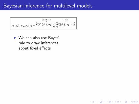
Bayesian inference for multilevel models
P({βi}, σb, σε|Y ) =
Likelihood︷ ︸︸ ︷P(Y |{βi}, σb, σε)
Prior︷ ︸︸ ︷P({βi}, σb, σε)
P(Y )
I We can also use Bayes’rule to draw inferencesabout fixed effects
I Computationally morechallenging than withsingle-level regression;Markov-chain MonteCarlo (MCMC) samplingtechniques allow us toapproximate it
560 580 600 620
68
1012
Intercept
neig
hbor
s
560 580 600 620
0.00
αα
P(αα
|Y)
4
6
8
10
12
14
0.00
P(αα|Y)
ββ
Why do you care???
I If you have had any training in psychology, you be askingyourself:
Do I really care about these models? For hypothesistesting I could do everything you just did with anANCOVA, treating participant as a random factor,or by looking at participant means.

Why do you care??? II
Do I really care about these models? For hypothesistesting I could do everything you just did with anANCOVA, treating participant as a random factor, orby looking at participant means.
I Yes, but there are several respects in which multi-level modelsgo beyond AN(C)OVA:
1. They handle imbalanced datasets just as well as balanceddatasets
2. You can use non-linear linking functions (e.g., logit models forbinary-choice data)
3. You can cross cluster-level effectsI Every trial belongs to both a participant cluster and an item
clusterI You can build a single unified model for inferences from your
dataI ANOVA requires separate by-participants and by-items
analyses (min-F ′ is quite conservative)
Why do you care??? II
Do I really care about these models? For hypothesistesting I could do everything you just did with anANCOVA, treating participant as a random factor, orby looking at participant means.
I Yes, but there are several respects in which multi-level modelsgo beyond AN(C)OVA:
1. They handle imbalanced datasets just as well as balanceddatasets
2. You can use non-linear linking functions (e.g., logit models forbinary-choice data)
3. You can cross cluster-level effectsI Every trial belongs to both a participant cluster and an item
cluster
I You can build a single unified model for inferences from yourdata
I ANOVA requires separate by-participants and by-itemsanalyses (min-F ′ is quite conservative)
Why do you care??? II
Do I really care about these models? For hypothesistesting I could do everything you just did with anANCOVA, treating participant as a random factor, orby looking at participant means.
I Yes, but there are several respects in which multi-level modelsgo beyond AN(C)OVA:
1. They handle imbalanced datasets just as well as balanceddatasets
2. You can use non-linear linking functions (e.g., logit models forbinary-choice data)
3. You can cross cluster-level effectsI Every trial belongs to both a participant cluster and an item
clusterI You can build a single unified model for inferences from your
data
I ANOVA requires separate by-participants and by-itemsanalyses (min-F ′ is quite conservative)
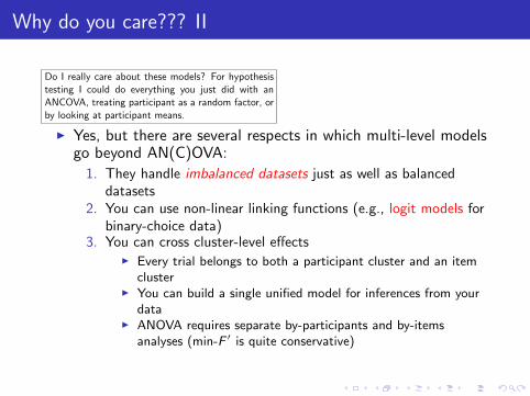
Why do you care??? II
Do I really care about these models? For hypothesistesting I could do everything you just did with anANCOVA, treating participant as a random factor, orby looking at participant means.
I Yes, but there are several respects in which multi-level modelsgo beyond AN(C)OVA:
1. They handle imbalanced datasets just as well as balanceddatasets
2. You can use non-linear linking functions (e.g., logit models forbinary-choice data)
3. You can cross cluster-level effectsI Every trial belongs to both a participant cluster and an item
clusterI You can build a single unified model for inferences from your
dataI ANOVA requires separate by-participants and by-items
analyses (min-F ′ is quite conservative)
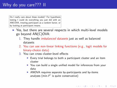
The logit link function for categorical data
I Much psycholinguistic data is categorical rather thancontinuous:
I Yes/no answers to alternations questionsI Speaker choice: (realized (that) her goals were unattainable)I Cloze continuations, and so forth. . .
I Linear models inappropriate; they predict continuous values
I We can stay within the multi-level generalized linear modelsframework but use different link functions and noisedistributions to analyze categorical data
I e.g., the logit model (Agresti, 2002; Jaeger, 2008)
ηij = α + βXij + bi (linear predictor)
ηij = logµij
1− µij(link function)
P(Y = y ;µij) = µij (binomial noise distribution)
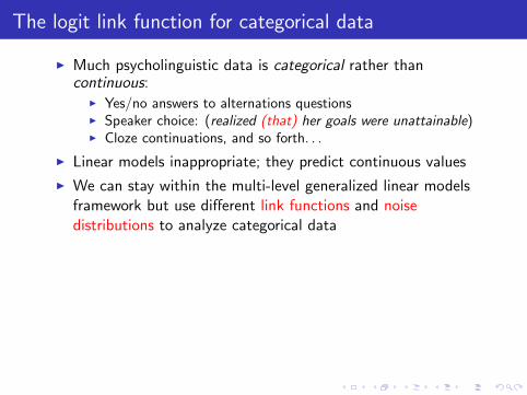
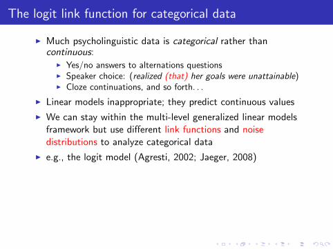
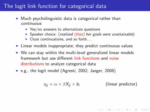
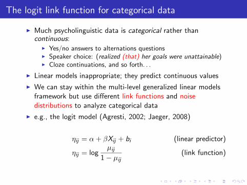
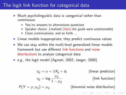
The logit link function for categorical data II
I We’ll look at the effect of neighborhood density on correctidentification as non-word in Bicknell et al. (2010)
I Assuming that any effect is linear in log-odds space (seeJaeger (2008) for discussion)
> lmer(correct ~ neighbors.scaled + (neighbors.scaled
| participant) + (1 | target), dat, family="binomial")
[...]
Random effects:
Groups Name Variance Std.Dev. Corr
participant (Intercept) 1.139785 1.06761
neighbors.scaled 0.030559 0.17481 -1.000
target (Intercept) 0.213311 0.46186
Number of obs: 1760, groups: participant, 44; target, 40
Fixed effects:
Estimate Std. Error z value Pr(>|z|)
(Intercept) 3.3593 0.2215 15.168 < 2e-16 ***
neighbors.scaled -0.6360 0.1271 -5.005 5.59e-07 ***
α̂—participants usually right
Σ̂bS (note there is no
σ̂ε for logit models)
σ̂bwβ̂—effect small compared with inter-subject variation
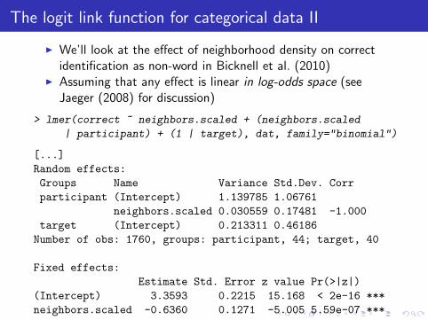
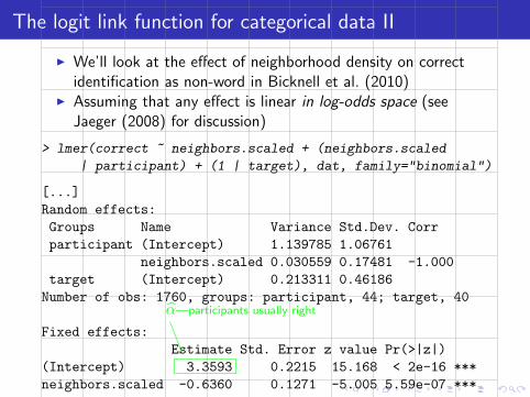
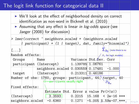
The logit link function for categorical data II
I We’ll look at the effect of neighborhood density on correctidentification as non-word in Bicknell et al. (2010)
I Assuming that any effect is linear in log-odds space (seeJaeger (2008) for discussion)
> lmer(correct ~ neighbors.scaled + (neighbors.scaled
| participant) + (1 | target), dat, family="binomial")
[...]
Random effects:
Groups Name Variance Std.Dev. Corr
participant (Intercept) 1.139785 1.06761
neighbors.scaled 0.030559 0.17481 -1.000
target (Intercept) 0.213311 0.46186
Number of obs: 1760, groups: participant, 44; target, 40
Fixed effects:
Estimate Std. Error z value Pr(>|z|)
(Intercept) 3.3593 0.2215 15.168 < 2e-16 ***
neighbors.scaled -0.6360 0.1271 -5.005 5.59e-07 ***
α̂—participants usually right
Σ̂bS (note there is no
σ̂ε for logit models)
σ̂bw
β̂—effect small compared with inter-subject variation
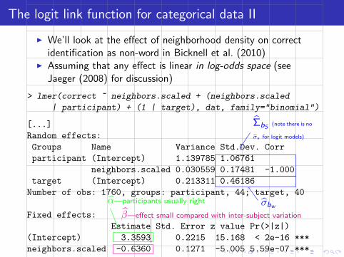
The logit link function for categorical data II
I We’ll look at the effect of neighborhood density on correctidentification as non-word in Bicknell et al. (2010)
I Assuming that any effect is linear in log-odds space (seeJaeger (2008) for discussion)
> lmer(correct ~ neighbors.scaled + (neighbors.scaled
| participant) + (1 | target), dat, family="binomial")
[...]
Random effects:
Groups Name Variance Std.Dev. Corr
participant (Intercept) 1.139785 1.06761
neighbors.scaled 0.030559 0.17481 -1.000
target (Intercept) 0.213311 0.46186
Number of obs: 1760, groups: participant, 44; target, 40
Fixed effects:
Estimate Std. Error z value Pr(>|z|)
(Intercept) 3.3593 0.2215 15.168 < 2e-16 ***
neighbors.scaled -0.6360 0.1271 -5.005 5.59e-07 ***
α̂—participants usually right
Σ̂bS (note there is no
σ̂ε for logit models)
σ̂bwβ̂—effect small compared with inter-subject variation
Summary thus far
I Hierarchical (multi-level, mixed-effects) models may seemstrange and foreign
I But all you really need to understand them is three basicthings
I Generalized linear modelsI The principle of maximum likelihoodI Bayesian inference
I These models open up many new interesting doors!

The good, the bad, and the ugly
I So now you have this new freedom in how to model your data!
I But this opens up many new choices you didn’t have before
I And if you make the wrong choices, you can draw the wronginferences from your dataset

The good, the bad, and the ugly
I So now you have this new freedom in how to model your data!
I But this opens up many new choices you didn’t have before
I And if you make the wrong choices, you can draw the wronginferences from your dataset
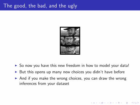
The good, the bad, and the ugly
I So now you have this new freedom in how to model your data!
I But this opens up many new choices you didn’t have before
I And if you make the wrong choices, you can draw the wronginferences from your dataset

A note on p-values and philosophy of science
I Frequentist hypothesis testing means the Neyman-Pearsonparadigm, with an asymmetry between null (H0) andalternative (H1) hypotheses
I A p-value from a dataset D is how unlikely a given datasetwas to be produced under H0
I Note that so-called “pMCMC” is NOT a p-value in theNeyman-Pearson sense!
I Weakness, both in practice and in principle: the alternativehypothesis is never actually used (except indirectly indetermining optimal acceptance and rejection regions)
A note on p-values and philosophy of science
I Alternative: Bayesian hypothesis testing, which is symmetric:
P(H0|D)
P(H1|D)=
P(D|H0)
P(D|H1)
P(H0)
P(H1)
I I am fundamentally Bayesian in my philosophy of science
I But, weakness in practice: your likelihoods P(D|H0) andP(D|H1) can depend on fine details of your assumptionsabout H0 and H1
I I do not trust you to assess these likelihoods neutrally! (Norshould you trust me)
I So for me, the p-value of your experiment serves as a roughindicator of how small P(D|H0) may be
I Technically, such a measure doesn’t need to be a trueNeyman-Pearson p-value (pMCMC falls into this category)
I really care about fixed effects—what random effects do Iuse?
I Simplest possible example: look at naming times of a set ofwords in high-predictability versus low-predictability contexts
I Treat as a dichotomous factor
I Quick review: what question are we asking when we dotraditional by-participants and by-items ANOVAs (t-tests)?
I Classic question: above and beyond idiosyncratic sensitivitiesof different individuals to context-driven predictability, arepredictable words in general named faster than unpredictablewords?
I In R:
RT ∼Is this coefficient < 0?︷ ︸︸ ︷Predictability+
idiosyncratic sensi-
tivities of different
individuals︷ ︸︸ ︷(Predictability|Subj)
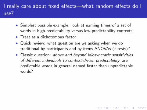
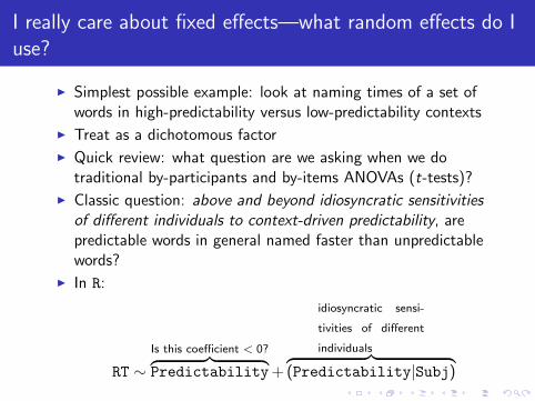

What random effects do I use?
I Now consider a 2× 2 design, where we want to assessinteraction of factors A and B in face of idiosyncraticsensitivities of both individuals and linguistic items toexperimental condition
I In R:
Response ∼ A ∗ B + (A ∗ B|Subj) + (A ∗ B|Item)
I Many of you may have had experience not being able to fitsuch a model to your data
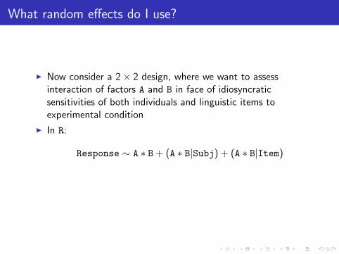
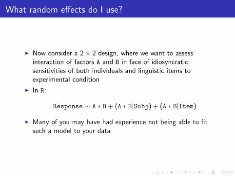
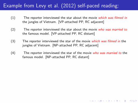
Example from Levy et al. (2012) self-paced reading:
(1) The reporter interviewed the star about the movie which was filmed inthe jungles of Vietnam. [VP-attached PP, RC adjacent]
(2) The reporter interviewed the star about the movie who was married tothe famous model. [VP-attached PP, RC distant]
(3) The reporter interviewed the star of the movie which was filmed in thejungles of Vietnam. [NP-attached PP, RC adjacent]
(4) The reporter interviewed the star of the movie who was married to thefamous model. [NP-attached PP, RC distant]
VP−attached PPRC adjacent
VP−attached PPRC distant
NP−attached PPRC adjacent
NP−attached PPRC distant
Res
idua
l RT
(m
s)
−200
−100
0
100
200
300
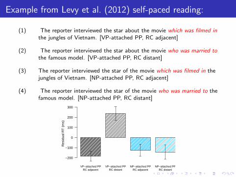
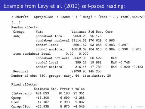
Example from Levy et al. (2012) self-paced reading:
> lmer(rt ~ Cprep*Cloc + (cond - 1 | subj) + (cond - 1 | item),REML=F)
[...]
Random effects:
Groups Name Variance Std.Dev. Corr
subj condabout local 9058.23 95.175
condabout nonlocal 29114.38 170.629 0.963
condof local 8661.62 93.068 0.983 0.897
condof nonlocal 10818.69 104.013 0.964 0.996 0.901
item condabout local 0.00 0.000
condabout nonlocal 3662.90 60.522 NaN
condof local 399.24 19.981 NaN -0.745
condof nonlocal 316.46 17.789 NaN 0.920 -0.423
Residual 21098.95 145.255
Number of obs: 880, groups: subj, 44; item.factor, 20
Fixed effects:
Estimate Std. Error t value
(Intercept) 424.823 18.193 23.351
Cprep -15.308 6.690 -2.288
Cloc 17.107 8.398 2.037
Cprep:Cloc -22.935 5.670 -4.045
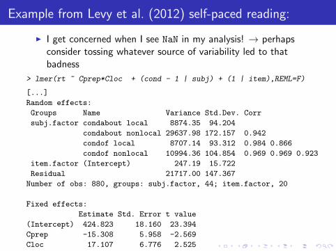
Example from Levy et al. (2012) self-paced reading:
I I get concerned when I see NaN in my analysis! → perhapsconsider tossing whatever source of variability led to thatbadness
> lmer(rt ~ Cprep*Cloc + (cond - 1 | subj) + (1 | item),REML=F)
[...]
Random effects:
Groups Name Variance Std.Dev. Corr
subj.factor condabout local 8874.35 94.204
condabout nonlocal 29637.98 172.157 0.942
condof local 8707.14 93.312 0.984 0.866
condof nonlocal 10994.36 104.854 0.969 0.969 0.923
item.factor (Intercept) 247.19 15.722
Residual 21717.00 147.367
Number of obs: 880, groups: subj.factor, 44; item.factor, 20
Fixed effects:
Estimate Std. Error t value
(Intercept) 424.823 18.160 23.394
Cprep -15.308 5.958 -2.569
Cloc 17.107 6.776 2.525
Cprep:Cloc -22.935 5.555 -4.129
> anova(m1, m2)
[...]
Df AIC BIC logLik Chisq Chi Df Pr(>Chisq)
m1 16 11461 11537 -5714.3
m2 25 11465 11585 -5707.6 13.553 9 0.1391
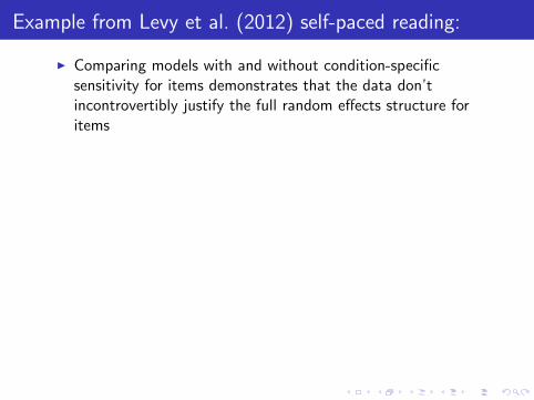
Example from Levy et al. (2012) self-paced reading:
I Comparing models with and without condition-specificsensitivity for items demonstrates that the data don’tincontrovertibly justify the full random effects structure foritems
> m1 <- lmer(rt ~ Cprep*Cloc + (cond - 1 | subj) + (1 | item))
> m2 <- lmer(rt ~ Cprep*Cloc + (cond - 1 | subj) + (cond - 1 | item))
> anova(m1,m2)
Df AIC BIC logLik Chisq Chi Df Pr(>Chisq)
m1 16 11461 11537 -5714.3
m2 25 11465 11585 -5707.6 13.538 9 0.1397
I This is a likelihood-ratio test between models
I Determining which random effects structure to use is theproblem of model selection
I The good news: model selection is extensively studied!
I The bad news: there are many, many models to be selectedfrom
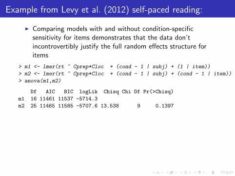
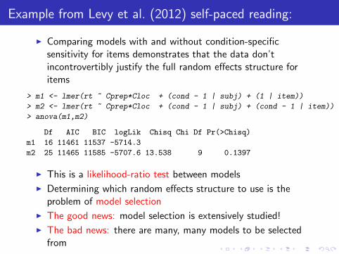
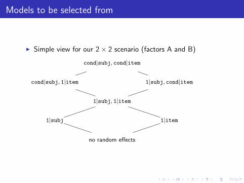
Models to be selected from
I Simple view for our 2× 2 scenario (factors A and B)
cond|subj, cond|item
cond|subj, 1|item 1|subj, cond|item
1|subj, 1|item
1|subj 1|item
no random effects
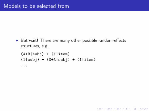
Models to be selected from
I But wait! There are many other possible random-effectsstructures, e.g.
(A+B|subj) + (1|item)
(1|subj) + (0+A|subj) + (1|item)
...
I What do these even mean?
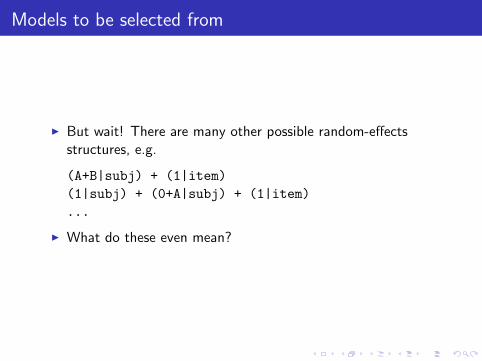
Models to be selected from
I But wait! There are many other possible random-effectsstructures, e.g.
(A+B|subj) + (1|item)
(1|subj) + (0+A|subj) + (1|item)
...
I What do these even mean?
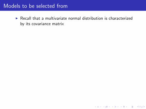
Models to be selected from
I Recall that a multivariate normal distribution is characterizedby its covariance matrix
I For two conditions A1, A2:
(A1 σ 1A2 1 σ
) (A1 σ1 1A2 1 σ2
)(1|subj) N/A (?)(
A1 σ1 0A2 0 σ2
) (A1 σ1 σ12
A2 σ12 σ2
)(1|subj) + (0 + A|subj) (but A mustbe recoded as numeric!)
(A|subj)
I If we add the possibility of no random effect, we get ahierarchy of 4 levels of richness
I With crossed participant and item random effects, 16 modelsin a lattice
I And the situation is much worse for more than two conditions
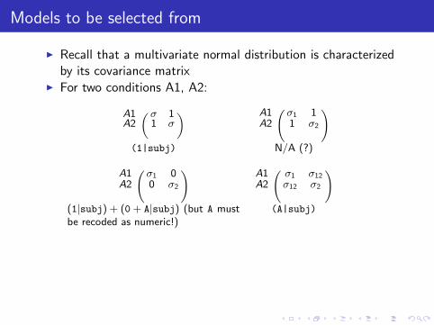
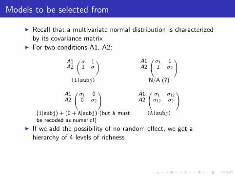
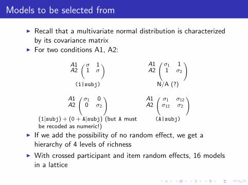
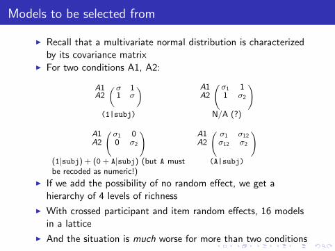
Which random effects do I use?
I I hope to have convinced you that you don’t want to domodel selection by hand
I Seems to me there are two reasonable things to do:
I Automate model selectionI Use different techniques that allow model selection to be
circumvented
I For the latter, we can use Bayesian inference to marginalizeover uncertainty regarding random effects
I Can’t do this in lme4 (yet?), but in the meantime we can useJAGS
I Ongoing joint work with Hal Tily: comparing these approaches
Which random effects do I use?
I I hope to have convinced you that you don’t want to domodel selection by hand
I Seems to me there are two reasonable things to do:I Automate model selection
I Use different techniques that allow model selection to becircumvented
I For the latter, we can use Bayesian inference to marginalizeover uncertainty regarding random effects
I Can’t do this in lme4 (yet?), but in the meantime we can useJAGS
I Ongoing joint work with Hal Tily: comparing these approaches
Which random effects do I use?
I I hope to have convinced you that you don’t want to domodel selection by hand
I Seems to me there are two reasonable things to do:I Automate model selectionI Use different techniques that allow model selection to be
circumvented
I For the latter, we can use Bayesian inference to marginalizeover uncertainty regarding random effects
I Can’t do this in lme4 (yet?), but in the meantime we can useJAGS
I Ongoing joint work with Hal Tily: comparing these approaches
Which random effects do I use?
I I hope to have convinced you that you don’t want to domodel selection by hand
I Seems to me there are two reasonable things to do:I Automate model selectionI Use different techniques that allow model selection to be
circumvented
I For the latter, we can use Bayesian inference to marginalizeover uncertainty regarding random effects
I Can’t do this in lme4 (yet?), but in the meantime we can useJAGS
I Ongoing joint work with Hal Tily: comparing these approaches
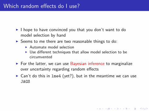
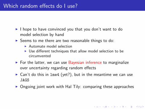
Rubric for comparing techniques
Types of datasets to look at:
I Balanced datasets closest to meeting the standards forANOVAs (=typical controlled psycholinguistic experiments)
I Balanced datasets where there are unbalanced controlvariables you’d like to incorporate into the analysis to improvesignal-to-noise ratio
I Imbalanced datasets that otherwise look like the above twocases;
I Imbalanced datasets with lots of potential predictors and/orcontrols
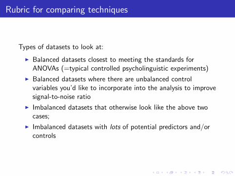
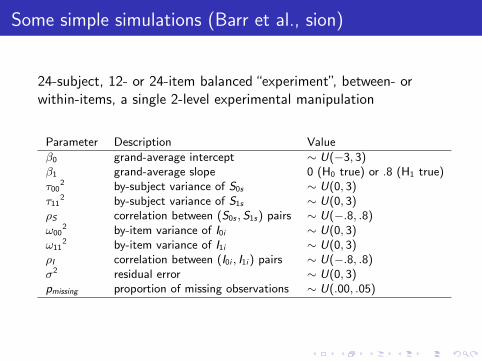
Some simple simulations (Barr et al., sion)
24-subject, 12- or 24-item balanced “experiment”, between- orwithin-items, a single 2-level experimental manipulation
Parameter Description Value
β0 grand-average intercept ∼ U(−3, 3)β1 grand-average slope 0 (H0 true) or .8 (H1 true)τ00
2 by-subject variance of S0s ∼ U(0, 3)τ11
2 by-subject variance of S1s ∼ U(0, 3)ρS correlation between (S0s , S1s) pairs ∼ U(−.8, .8)ω00
2 by-item variance of I0i ∼ U(0, 3)ω11
2 by-item variance of I1i ∼ U(0, 3)ρI correlation between (I0i , I1i ) pairs ∼ U(−.8, .8)σ2 residual error ∼ U(0, 3)pmissing proportion of missing observations ∼ U(.00, .05)
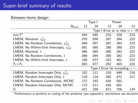
Super-brief summary of results
Between-items design:Type I Power
Nitems 12 24 12 24 12 24
Type I Error at or near α = .05
min-F ′ .044 .045 .210 .328 .210 .328LMEM, Maximal, χ2
LR .070 .058 .267 .364 .223 .342LMEM, No Random Correlations, χ2
LR .069 .057 .267 .363 .223 .343LMEM, No Within-Unit Intercepts, χ2
LR .081 .065 .288 .380 .223 .342LMEM, Maximal, t .086 .065 .300 .382 .222 .343LMEM, No Random Correlations, t .086 .064 .300 .382 .223 .343LMEM, No Within-Unit Intercepts, t .100 .073 .323 .401 .222 .342F1×F2 .063 .077 .252 .403 .224 .337
Type I Error far exceeding α = .05
LMEM, Random Intercepts Only, χ2LR .102 .111 .319 .449 .216 .314
LMEM, Random Intercepts Only, t .128 .124 .360 .472 .217 .314LMEM, No Random Correlations, MCMC .172 .192 .426 .582LMEM, Random Intercepts Only, MCMC .173 .211 .428 .601F1 .421 .339 .671 .706 .134 .212∗Performance is sensitive to coding of the predictor (see appendix); simulations use deviation coding
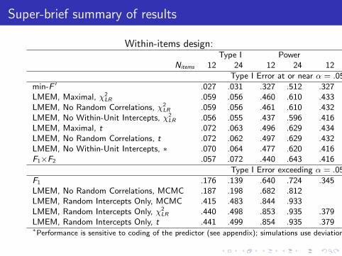
Super-brief summary of results
Within-items design:Type I Power
Nitems 12 24 12 24 12 24
Type I Error at or near α = .05
min-F ′ .027 .031 .327 .512 .327 .512LMEM, Maximal, χ2
LR .059 .056 .460 .610 .433 .591LMEM, No Random Correlations, χ2
LR .059 .056 .461 .610 .432 .593LMEM, No Within-Unit Intercepts, χ2
LR .056 .055 .437 .596 .416 .579LMEM, Maximal, t .072 .063 .496 .629 .434 .592LMEM, No Random Correlations, t .072 .062 .497 .629 .432 .593LMEM, No Within-Unit Intercepts, ∗ .070 .064 .477 .620 .416 .580F1×F2 .057 .072 .440 .643 .416 .578
Type I Error exceeding α = .05
F1 .176 .139 .640 .724 .345 .506LMEM, No Random Correlations, MCMC .187 .198 .682 .812LMEM, Random Intercepts Only, MCMC .415 .483 .844 .933LMEM, Random Intercepts Only, χ2
LR .440 .498 .853 .935 .379 .531LMEM, Random Intercepts Only, t .441 .499 .854 .935 .379 .531∗Performance is sensitive to coding of the predictor (see appendix); simulations use deviation coding
Tentative initial conclusions
I Wisdom of the crowd: for traditional, perfectly balanceddatasets, you lose relatively little with standard ANOVAscontrolled studies
I In practice, I think most researchers informally pay attention tomax(F1,F2)
I Clark (1973) warned that this is anticonservative, but much ofthis anticonservativity seems to be in principle only (though seeour results regarding dependence on sizes of random effects)
I Failing to include appropriate random-effects structure in yourmodel is horribly anti-conservative!
I Both model selection and fully Bayesian analysis can addressthis problem
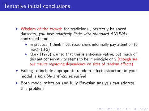

So why did I care about hierarchical models again?
I If all you ever work with is perfectly balanced factorial designs,then you’re probably OK with ANOVAs
I (On the other hand, when was the last time you tested forsphericity and considered using Hotelling’s T 2 test?)
I You may be able to eke out a bit more statistical power inthese studies from the hierarchical analysis; but be sure thatyou are not hallucinating that power!
I Hierarchical models really come into their own, however, with
I Imbalanced datasetsI Appreciably non-linear responsesI Injection of prior knowledge into (Bayesian) data analysisI Flexibility in specification of the model structure
I More generally, establishing proper standards for use ofhierarchical models on linguistic data opens a channel to arich universe of data-analysis techniques
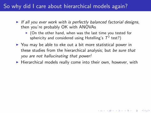
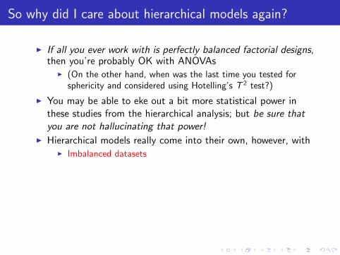
So why did I care about hierarchical models again?
I If all you ever work with is perfectly balanced factorial designs,then you’re probably OK with ANOVAs
I (On the other hand, when was the last time you tested forsphericity and considered using Hotelling’s T 2 test?)
I You may be able to eke out a bit more statistical power inthese studies from the hierarchical analysis; but be sure thatyou are not hallucinating that power!
I Hierarchical models really come into their own, however, withI Imbalanced datasets
I Appreciably non-linear responsesI Injection of prior knowledge into (Bayesian) data analysisI Flexibility in specification of the model structure
I More generally, establishing proper standards for use ofhierarchical models on linguistic data opens a channel to arich universe of data-analysis techniques
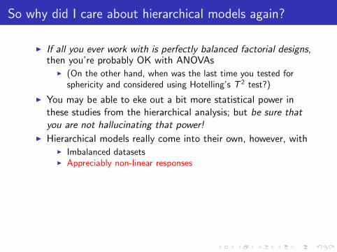
So why did I care about hierarchical models again?
I If all you ever work with is perfectly balanced factorial designs,then you’re probably OK with ANOVAs
I (On the other hand, when was the last time you tested forsphericity and considered using Hotelling’s T 2 test?)
I You may be able to eke out a bit more statistical power inthese studies from the hierarchical analysis; but be sure thatyou are not hallucinating that power!
I Hierarchical models really come into their own, however, withI Imbalanced datasetsI Appreciably non-linear responses
I Injection of prior knowledge into (Bayesian) data analysisI Flexibility in specification of the model structure
I More generally, establishing proper standards for use ofhierarchical models on linguistic data opens a channel to arich universe of data-analysis techniques
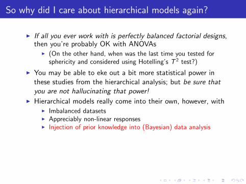
So why did I care about hierarchical models again?
I If all you ever work with is perfectly balanced factorial designs,then you’re probably OK with ANOVAs
I (On the other hand, when was the last time you tested forsphericity and considered using Hotelling’s T 2 test?)
I You may be able to eke out a bit more statistical power inthese studies from the hierarchical analysis; but be sure thatyou are not hallucinating that power!
I Hierarchical models really come into their own, however, withI Imbalanced datasetsI Appreciably non-linear responsesI Injection of prior knowledge into (Bayesian) data analysis
I Flexibility in specification of the model structure
I More generally, establishing proper standards for use ofhierarchical models on linguistic data opens a channel to arich universe of data-analysis techniques
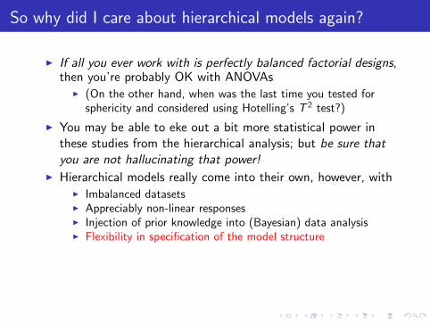
So why did I care about hierarchical models again?
I If all you ever work with is perfectly balanced factorial designs,then you’re probably OK with ANOVAs
I (On the other hand, when was the last time you tested forsphericity and considered using Hotelling’s T 2 test?)
I You may be able to eke out a bit more statistical power inthese studies from the hierarchical analysis; but be sure thatyou are not hallucinating that power!
I Hierarchical models really come into their own, however, withI Imbalanced datasetsI Appreciably non-linear responsesI Injection of prior knowledge into (Bayesian) data analysisI Flexibility in specification of the model structure
I More generally, establishing proper standards for use ofhierarchical models on linguistic data opens a channel to arich universe of data-analysis techniques
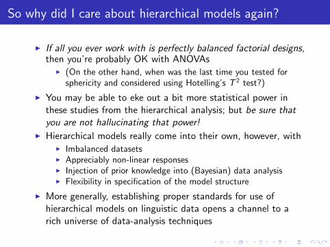
So why did I care about hierarchical models again?
I If all you ever work with is perfectly balanced factorial designs,then you’re probably OK with ANOVAs
I (On the other hand, when was the last time you tested forsphericity and considered using Hotelling’s T 2 test?)
I You may be able to eke out a bit more statistical power inthese studies from the hierarchical analysis; but be sure thatyou are not hallucinating that power!
I Hierarchical models really come into their own, however, withI Imbalanced datasetsI Appreciably non-linear responsesI Injection of prior knowledge into (Bayesian) data analysisI Flexibility in specification of the model structure
I More generally, establishing proper standards for use ofhierarchical models on linguistic data opens a channel to arich universe of data-analysis techniques

References I
Agresti, A. (2002). Categorical Data Analysis. Wiley, second edition.
Baayen, R. H., Davidson, D. J., and Bates, D. M. (2008). Mixed-effectsmodeling with crossed random effects for subjects and items. Journalof Memory and Language, 59(4):390–412.
Barr, D. J., Levy, R., Scheepers, C., and Tily, H. J. (In revision). Randomeffects structure in mixed-effects models: Keep it maximal. Availableonline at http://idiom.ucsd.edu/~rlevy/papers/barr-levy-scheepers-tily-8-aug-2011-submitted.pdf.
Bicknell, K., Elman, J. L., Hare, M., McRae, K., and Kutas, M. (2010).Effects of event knowledge in processing verbal arguments. Journal ofMemory and Language, 63:489–505.
Clark, H. H. (1973). The language-as-fixed-effect fallacy: A critique oflanguage statistics in psychological research. Journal of VerbalLearning and Verbal Behavior, 12:335–359.
Jaeger, T. F. (2008). Categorical data analysis: Away from ANOVAs(transformation or not) and towards logit mixed models. Journal ofMemory and Language, 59(4):434–446.

References II
Levy, R., Fedorenko, E., Breen, M., and Gibson, T. (2012). Theprocessing of extraposed structures in English. Cognition,122(1):12–36.